Some fundamentals of numerical weather prediction

(for ATM 562)

Robert FovellAtmospheric and Environmental Sciences

University at Albany, SUNY

rfovell@albany.edu

Equations

• Navier-Stokes equations– Newton’s 2nd law: real & apparent forces– Turbulence and mixing

• 1st law of thermodynamics

• Ideal gas law

• Continuity equation

• Clausius-Clapeyron equation

Domain

• Local, regional or global in scale

Domain

• Local, regional or global in scale

• Discretize into grid volumes– virtual internal walls– boundary conditions

• Initialize each volume• Make some forecasts…

Extrapolation

• Equations predict tendencies

– Initial forecasts start with observations but subsequent forecasts based on forecasts

– Forecasts used to recalculate tendencies– Success depends on quality of initialization and

accuracy of tendencies

A simplistic example:temperature in your backyard

The model forecast will consider an enormous number of factors to estimate present tendency to project future

value

In the absence of such information, you simply guess… and wait to see how good your guess was.

The model does not wait. It uses each forecast to recalculate the tendencies to make the next forecast

Verification of your forecast:OK since you didn’t project out too far

Forecast time steps cannot be too long.Tendencies have the tendency to CHANGE.

Model forecasts will reflect…

• Radiative processes• Surface and sub-surface processes• Cloud development and microphysics• Advection and mixing• Convergence and divergence• Ascent and subsidence• Sea-breezes, cold and warm fronts• Cyclones, anticyclones, troughs, ridges

Model resolution

• Things to try to resolve– Clouds, mountains, lakes & rivers,

hurricane eyes and rainbands, fronts & drylines, tornadoes, much more

• What isn’t resolved is subgrid• At least 2 grid boxes across a feature for

model to even “see” it… and at least 6 to render it properly

Wave-like features are ubiquitous,in space and time

Models sample a wave only at grid points.Example: 4 points across each wave.

Models “connect the dots”.

Suppose we have only 3 points across the wave…or just 2 points…

These do not look much like the actual wave at all.With only 2 points, wave may be invisible.

High resolution Hurricane Katrina satellite picture = composed of 1 km pixels.

High resolution model = possibly accurate, definitely expensive,and extremely time-consuming

As model resolution increases, we see more, but have to DO more.Plus, the time step has to decrease, to maintain linear stability

Compromising on the resolution – now it’s 10 km

30 km resolution

At what point would we not be able to tell that’s a hurricane if we had not known it from the start?

This is the world as seen by global weather models not so long ago, and many climate models today.

“My favorite story is about the model that perfectly predicts tomorrow’s weather, but it takes two days to run the program.”

Outlook is good…

• Models are improving– Faster computers– More and better input data (satellites)– Better ways of using those data– Progressively better numerical techniques– High resolution models… so less is missed

(subgrid)– … but some things we can never capture

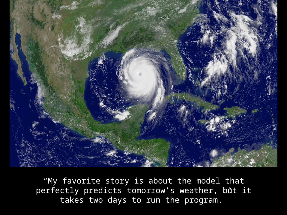
Parameterization

• Parameterization = an attempt to represent what we cannot see, based largely on what we can

• Parameterizations in a typical NWP model include - and are NOT limited to…– Boundary layer processes and subgrid mixing– Cloud microphysics [resolve cloud, can’t resolve drops]– Convective parameterizations [can’t resolve clouds]– Surface processes [heat, moisture fluxes]– Subsurface processes [soil model, ocean layers]– Radiative transfer, including how radiation interacts with

clouds

• Here is an example…

Another view of Katrina... But focusing on roll clouds.Roll clouds are revealing of boundary layer mixing.

How roll clouds form

•Consider the sun warming the land during the day

How roll clouds form

• With uneven heating, wind and vertical wind shear, roll-like circulations can start

• You can simulate roll formation in a high resolution model (∆x ≤ 500 m)

How roll clouds form

• As the land warms up, the rolls get deeper (also wider)

• The rolls mix heat vertically – air is a lousy conductor

• Also mixing momentum, moisture

How roll clouds form

• If conditions are favorable, clouds will form above the roll updrafts

• These make the rolls visible

• We see these roll clouds on satellite pictures

• In a sense, being able to simulate the roll clouds means we’ve done many things well -- radiation, winds, mixing, surface/soil and saturation processes

Parameterizing mixing…

• In many models, however, the roll clouds and the mixing that created them are subgrid (and if they DO appear, they are almost certainly mishandled)

• But that mixing is important. It influences structure and stability of the atmosphere, including CAPE, CIN and convective initiation

• If we cannot resolve it, we must parameterize it• NWP models are full of parameterizations, each a

potential model shortcoming, each a possible source of problems, of error, of uncertainty regarding the future

Birth of NWP

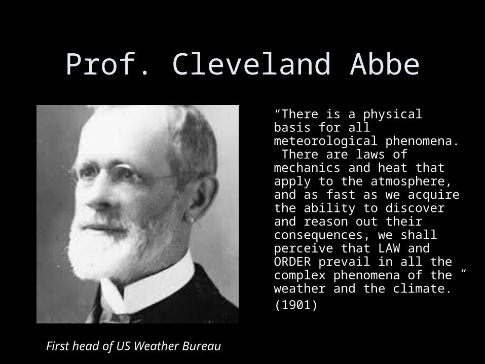
Prof. Cleveland Abbe

“There is a physical basis for all meteorological phenomena. There are laws of mechanics and heat that apply to the atmosphere, and as fast as we acquire the ability to discover and reason out their consequences, we shall perceive that LAW and ORDER prevail in all the complex phenomena of the weather and the climate.”(1901)

First head of US Weather Bureau

Prof. Vilhelm Bjerknes

• 1904 vision on weather prediction

• Lamented the “unscientific” basis of meteorology

• Goal: to make meteorology a more exact science

• … by making predictions

Bjerknes’ vision

• Two key ingredients:– Sufficiently accurate knowledge of the state of the

atmosphere at the initial time– Sufficiently accurate knowledge of the physical laws that

govern how the atmospheric state evolves

• Identified 7 fundamental variables -- T, p, density, humidity, and three wind components -- and the equations that calculated their tendencies

• These are nasty equations, without simple solutions. Only numerical methods could be brought to bear on them.

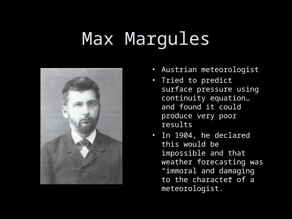
Max Margules

• Austrian meteorologist• Tried to predict surface

pressure using continuity equation… and found it could produce very poor results

• In 1904, he declared this would be impossible and that weather forecasting was “immoral and damaging to the character of a meteorologist.”

Lewis Fry Richardson

• Among first to try to solve the weather/climate equations numerically

• Invented many concepts still used today

• Made the first numerical weather forecast

• Prediction was horribly wrong

Richardson’s technique

• Richardson laid out a grid, collected his observations, created novel numerical approximations for his equations and crunched his numbers, by hand and slide rule

• Actually, it was a hindcast that took laborious computations using old, tabulated data

dreamstime.com

Aside

• “In 1967, Keuffel & Esser, commissioned a study of the future. The report predicted that, by the year 2067, Americans would live in domed cities… and watch three-dimensional television. Unfortunately for the company, the report failed to predict that slide rules would be obsolete in less than ten years.”

Richardson’s grid

Richardson used 5 vertical levels, including surface

Richardson’s forecast

• He predicted a surface pressure rise of 145 mb (about 14%) in only 6 h

• In reality the pressure hardly changed at all

• First forecast = first forecast failure• What went wrong?

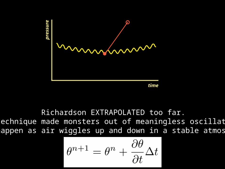
Richardson EXTRAPOLATED too far.His technique made monsters out of meaningless oscillations

that happen as air wiggles up and down in a stable atmosphere.

Richardson’s book

• Richardson revealed the details of his blown forecast in “Weather Prediction by Numerical Process”, published in 1922.

• Undaunted, he imagined his pencil and paper technique applied to the entire global atmosphere…– In a huge circular ampitheatre in which human

calculators would do arithmetic and, guided by a conductor at the center, pass results around to neighbors

Richardson’s forecasting theater

After Richardson

• Richardson’s confidence was not unfounded.• Mathematicians and meteorologists realized the flaws

of his techniques • The digital computer was created • The meteorological observation network was

expanding rapidly• It seemed only a matter of time until the vision of

Abbe, the goal of Bjerknes, the dream of Richardson, became a reality…

• Then in 1962, Ed Lorenz did his little experiment…

Prof. Ed Lorenz

• MIT professor• Landmark 1962

paper “Deterministic Nonperiodic Flow”

• Led to “chaos theory” and dynamical systems

• Associated with “butterfly effect”

The Lorenz Experiment

• Lorenz’ model wasn’t a weather model, and didn’t even have grid points

• 3 simple equations, which can describe fluid flow in a cylinder with heated bottom and cooled top

• He called his variables X, Y and Z

The Lorenz Experiment

• X indicated the magnitude and direction of the overturning motion

• As X changed sign, the fluid circulation reversed

The Lorenz Experiment

• Y was proportional to the horizontal T gradient

The Lorenz Experiment

• And Z revealed the fluid’s stability

The Lorenz Model

• Three simple equations• But in important ways

they were like the equations we use in weather forecasting– They are coupled– They are nonlinear

Simulation similar to Lorenz’ original experiment.X = circulation strength & magnitude.

The model was started with unbalanced initial values for X, Y and Z, creating a shock. The model was seeking a

suitable balance.

Next, a spin-up period with swings that grow until…

The fluid chaotically shifts from CW to CCW circulations in an nonperiodic fashion

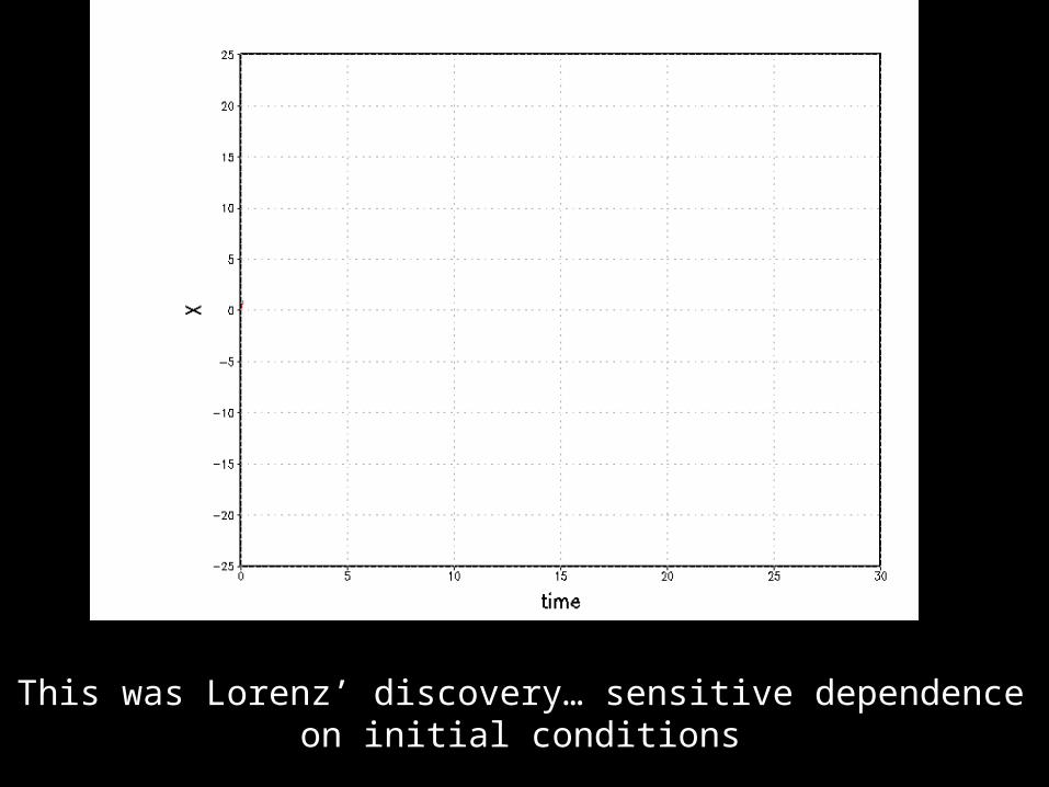
This was Lorenz’ discovery… sensitive dependenceon initial conditions

Dependence on initial conditions

• Caused by nonlinear terms• Even if model is perfect, any error in initial

conditions means forecast skill decreases with time

• Reality: models are far from perfect• Long range weather prediction is impossible• Lorenz: “We certainly hadn’t been successful at

doing that anyway and now we had an excuse.”

From Lorenz (1963)

• “Two states differing by imperceptible amounts may eventually evolve into two considerably different states. If, then, there is any error whatever in observing the present state — and in any real system such errors seem inevitable — an acceptable prediction of an instantaneous state in the distant future may well be impossible.”

From Lorenz (1963)

• “In view of the inevitable inaccuracy and incompleteness of weather observations, precise very-long-range forecasting would seem to be non-existent…. There remains the very important question as to how long is ‘very-long-range’. Our results do not give the answer for the atmosphere; conceivably it could be a few days or a few centuries.”

Lorenz attractor

• 3D space with coordinates being the Lorenz variables, X Y and Z

• Predicted values can be plotted as a point in this space

• Start with an initial conditions that are slightly different…,

• … they diverge in this space• Birth of chaos theory• Poorly named: chaos ≠

randomWikipedia

The butterfly metaphor

• ‘Butterfly effect’ did not originate w/ Lorenz. In a 1963 paper, he referred to seagulls.

• In 1969, Joe Smagorinsky wrote “would the flutter of a butterfly’s wings ultimately amplify to the point where numerical simulation departs from reality?” (BAMS article)

• In 1993, Lorenz gave a talk entitled, “Does the flap of a butterfly’s wings in Brazil stir up a tornado in Texas?”. But, Lorenz did not write the title.

• ‘Butterfly effect’ was coined by James Gleick in his 1987 book, “Chaos: Making a New Science”

Summary

• NWP models = great tools for understanding our present and predicting our future

• Models initialized with data to compute tendencies, via approximation combined with extrapolation

• Models have limitations– Resolution– Unresolvable features and processes– Incomplete or erroneous initial conditions

• New forecasts based on previous ones, so error grows

• Limit to predictability (Lorenz)

[end]