Some considerations on state equations of linear active networks

CIRCUIT THEORY AND APPLICATIONS, VOL. 2. 39-50 (1974)

SOME CONSIDERATIONS ON STATE EQUATIONS OF LINEAR ACTIVE NETWORKS

KOTARO HIRANO, FUMIAKI NISHI, AND SHIN-ICHIRO TOMIYAMA Department of Electronic Engineering, Kobe University, Rokko, Nada, Kobe, Japan

SUMMARY

I t is shown that if there equivalently exist the virtual resistive elements in parallel with the inductive elements of the overnormal tree of a given linear active network or in series with the capacitive elements of the corresponding co-tree, an increase in the number of state variables arises. It is also shown that when a virtual resistor equivalently appears in parallel with the distinct resistor in a tree or in series with the distinct resistor in the co-tree, a decrease in the number of state variables may arise. This is, however, a rare case in the usual types of network.

Two algebraic methods for obtaining the state equation of linear active networks are presented. One is useful for the networks in which the decrease in the number of state variables does not arise. From the other, the output equation for the required variables is obtained at the same time as the state equation. Further, the initial values are simply determined without iteration in many cases.

INTRODl ICTION

Recently, with the development of integration techniques, much attention has been concentrated on active networks, and the state-variable approach has served as an effective technique for analyzing these networks' as well as passive ones. For passive networks, the state-variable approach was first introduced by Ba~hkow. ' .~ The derivations of state equation from the Lagrangian formulation and the mixed equation were also accom- p l i ~ h e d . ~ . ~ Extensions of the state-variable approach to active networks have been attempted by many author^.^-^ The algebraic method for obtaining the state equations has also been A major problem in obtaining the state equation of active networks in a general form is due to the difficulty in finding the order of complexity or finding the state variable^.^.'^ The problem of finding the order of complexity of active networks is important not only from the theoretical but also the practical point of view in the derivation of state equation by digital computer. Unlike linear passive RLC networks, all the voltages of the capacitive elements in the overnormal tree7 and all the currents of the inductive elements in the corresponding co-tree are not always chosen as state variables. In some cases, several voltages (or currents) of the inductive elements in the overnormal tree and several currents (or voltages) of the capacitive elements in the corresponding co-tree remain as state variables implying an increase in the number of state variables. Whereas, in a few other rare cases, several voltages of the capacitive elements in the overnormal tree and several currents of the inductive elements in the corresponding co-tree d o not remain as state variables leading to a decrease in the number of state variables.

Formulations of the output equation and the initial values of the state variables are also important as well as that of the state equation to evaluate the transient response of linear active networks. In References 12-14 the voltages or currents of all the elements are regarded as the output. But in practical application, it is not always required to determine all of them. The initial-value problem in linear RLCM networks was first discussed by Seshu and Balabanian,' and was extended to linear active networks by Derv i~o&'~ for the general case. But the latter method requires iterative calculations.

In this paper considerations in the number of state variables of linear active networks are first carried out by introducing the virtual resistive elements. Then, an algebraic method is presented for obtaining the state equation in the case where a decrease in the number of state variables does not arise. Further, the general

Received 28 December 1972 Revised 10 July 1973

0 1974 by John Wiley & Sons, Lld

39

40 KOTARO HIRANO, FUMIAKI NISHI, AND SHIN-ICHIRO TOMIYAMA

=

algebraic method for obtaining the state equation and output equation of linear active networks at the same time is described and under the assumption of D e r v i ~ o i l u ’ ~ the initial values are simply determined without iterative calculations in many cases.

- - -Es Fss, Fsc 0 0 S

- E R F R S , FRC FRG 0 R

--&” FS”S, Fs,c FS”, FSJ s u

- E L FLS, FLC FLr

- Q J E Jl, Jz JG‘ J F J

NETWORK DESCRIPTION AND STATE EQUATION

Network description

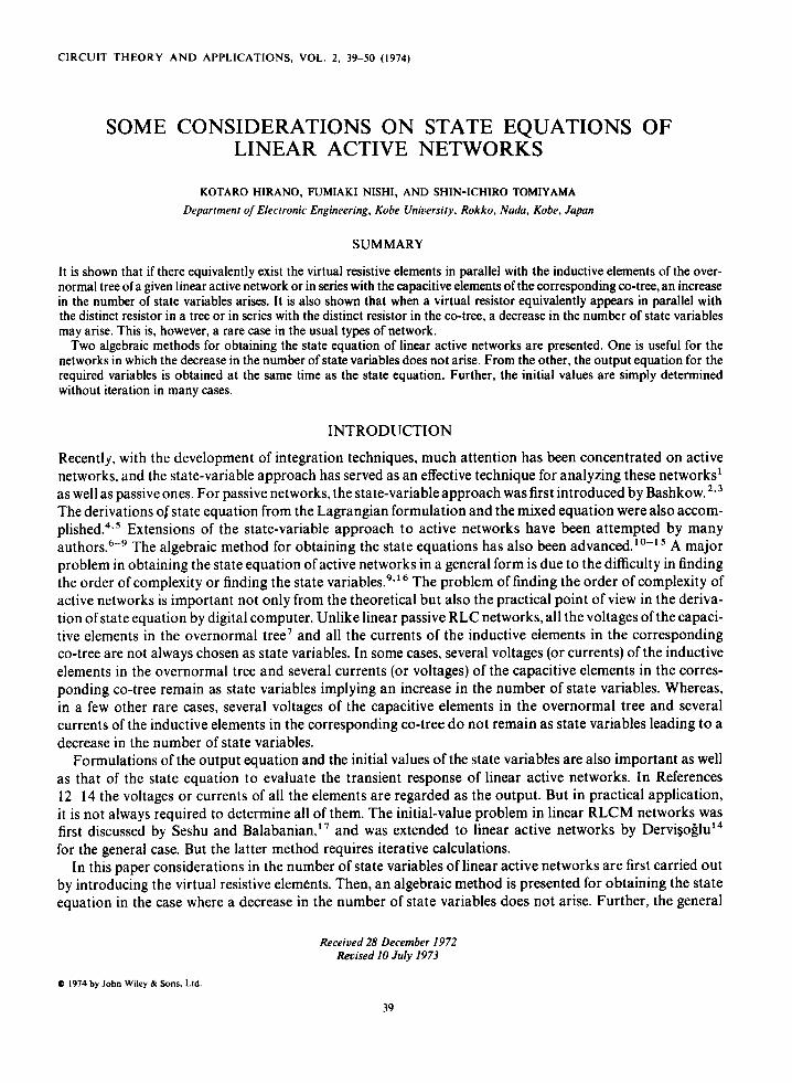
This paper is restricted to networks having (a) no loops composed of independent voltage sources E, controlled voltage sources, and current sensors only and (b) no cut-set composed of independent current sources J , controlled current sources, and voltage sensors only. Thus the network, N can be constructed of the following five types of branches and independent sources.

(a) Su-branch : A series connection of a voltage sensor with a controlled voltage source E,. (b) &-branch: A parallel connection of a current sensor with a controlled current source J,. (c) C-branch : A series connection ofa capacitor with E, in a co-tree, or a parallel connection of a capacitor

(d) R-branch: A branch given by replacing ‘capacitor’ in the C-branch with ‘resistor’. (e) L-branch: A branch given by replacing ‘capacitor’ in the C-branch with ‘inductor’. The Su-, Si-, and C-branches are shown in Figure l(a), (b), and (c), respectively. In the following, the

currents through all the links and the voltages across all the tree branches are chosen as the branch variables. Then, for example, the currents of C-branches in a co-tree are identical with those of capacitors, and the voltages of C-branches in a tree with those of capacitors.

with J , in a tree.

(0) (b) ( C )

Figure 1. Branch structures. (a) So-branch (b) S,-branch (c) C-brarrch (1) in a co-tree (2) in a tree

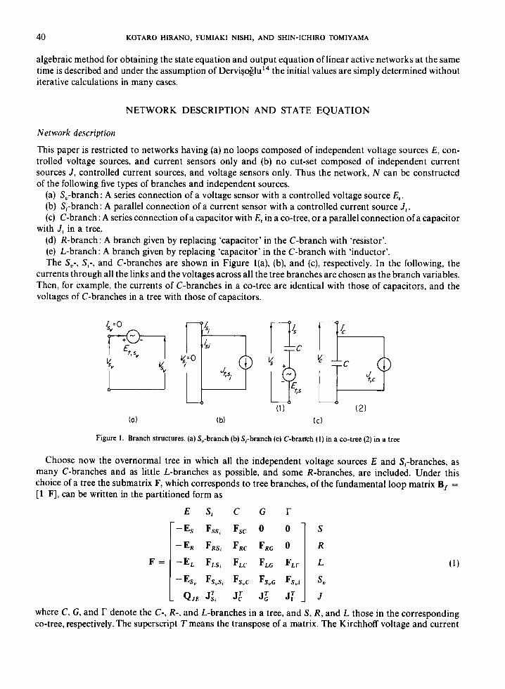
Choose now the overnormal tree in which all the independent voltage sources E and &-branches, as many C-branches and as little L-branches as possible, and some R-branches, are included. Under this choice of a tree the submatrix F, which corresponds to tree branches, of the fundamental loop matrix B, = [l F], can be written in the partitioned form as

E S ~ c G r

SOME CONSIDERATIONS ON STATE EQUATIONS OF LINEAR ACTIVE NETWORKS 41

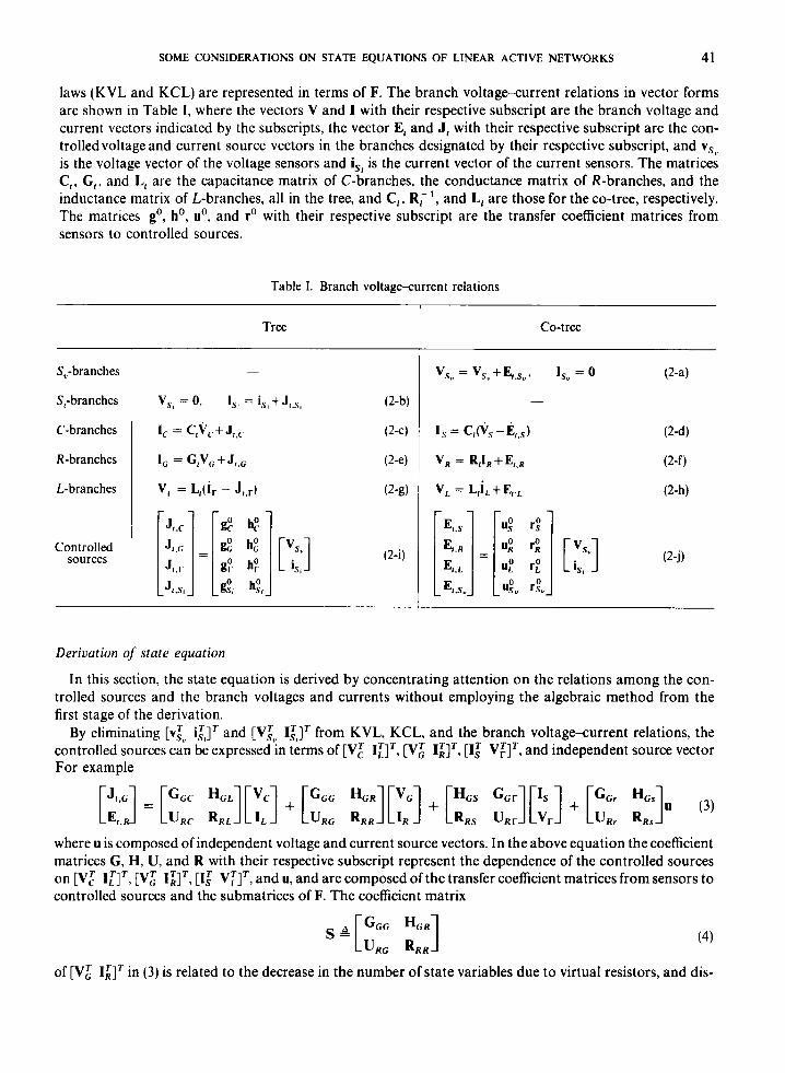
laws (KVL and KCL) are represented in terms of F. The branch voltage-current relations in vector forms are shown in Table I , where the vectors V and I with their respective subscript are the branch voltage and current vectors indicated by the subscripts, the vector E, and J, with their respective subscript are the controlled voltage and current source vectors in the branches designated by their respective subscript, and vs, is the voltage vector of the voltage sensors and is, is the current vector of the current sensors. The matrices C,, G , , and L, are the capacitance matrix of C-branches, the conductance matrix of R-branches, and the inductance matrix of L-branches, all in the tree, and C,, R; ', and L, are those for the co-tree, respectively. The matrices go, ho, uo, and ro with their respective subscript are the transfer coefficient matrices from sensors to controlled sources.

Table I. Branch voltage-current relations

S,-branches

Si-branches

C-branches

R-branches

L-branches

Controlled sources

Tree Co-tree

'R = R,lR + E ~ . R

VL = L,IL+EI.L

Derivation of state equation

In this section, the state equation is derived by concentrating attention on the relations among the controlled sources and the branch voltages and currents without employing the algebraic method from the first stage of the derivation.

By eliminating [vs', i:,]' and [V:" I:,]' from KVL, KCL, and the branch voltage-current relations, the controlled sources can be expressed in terms of [V,' I:]', [V,' I:]', [I: VF]', and independent source vector For example

where u is composed of independent voltage and current source vectors. In the above equation the coefficient matrices G , H, U, and R with their respective subscript represent the dependence of the controlled sources on [V,' I[]', [Vz I;]', [I: VF]', and u, and are composed of the transfer coefficient matrices from sensors to controlled sources and the submatrices of F. The coefficient matrix

of [V,' I;]' in (3) is related to the decrease in the number of state variables due to virtual resistors, and dis-

42 KOTARO HIRANO, FUMIAKA NISHI, AND SHIN-ICHIRO TOMIYAMA

cussed in the following section. If the matrix

is nonsingular, then from KVL concerned with the fundamental loops determined by R, KCL concerned with the fundamental cut-sets determined by G, and the branch voltage-current relations of R and G, [V,' I;]' is expressed in terms of [V,' I:]', [I: VF]'. and u. The matrix J is singular when a decrease in the number of state variables due to virtual resistors arises. This situation is a rare case, and is discussed in the following. When J is nonsingular the controlled sources can be expressed in terms of [V,' I l lT, [I: V;]', and u. For example it follows

where the matrices with asterisk are the ones representing the dependence of [Ets J;r]' on [Vc T I T L] T , [I: V;IT, and u, and composed of GI, R, , the transfer coefficient matrices from sensors to controlled sources, and the submatrices of F. The coefficient matrix

of [I: VF]' in (6) is related to the increase in the number of state variables due to virtual resistive elements, and this is discussed in the following section.

Further elimination of unwanted variables yields the equation

whereX = [V,' I:lTand Z = [I: VFIT,andA, = [C, + L,]T,A4 = C, + LI, andothercoefficientmatrices of (8) are determined from KVL, KCL, and the branch voltage-current relations. The notation 4- represents the direct sum of matrices.

When T is nonsingular, multiplying (8) from the left side by the inverse of the coefficient matrix of [ZT XTIT yields the state equation in terms of state vector [Z' XTIT, i.e., all the voltages of C-branches and L-branches in a tree, and all the currents of C-branches and L-branches in the corresponding co-tree. When T is singular, the algebraic method is required for obtaining the state equation. Especially for T = 0, the state equation with respect to the state vector X, i.e., the voltages of C-branches in a tree and the currents of L-branches in the corresponding co-tree, is obtained if (C, + L,) + B,A2 is nonsingular. The last case is the case where the normal tree* for the RC network with controlled sources can be chosen.

The following procedure is useful for singular T to obtain the state equation from (8) in the case where the decrease in the number of state variables does not arise.

Find the nonsingular matrix R, such as a l l

where a and b are the rank and the nullity of A, in (8), respectively. Multiply the first-row matrix equation of (8) from the left side by R, . Then it becomes

where 2, consists of the first a elements of Z, and Z, consists of the remaining elements of Z. Note that the rank of [B13 B,,] is equal to p.


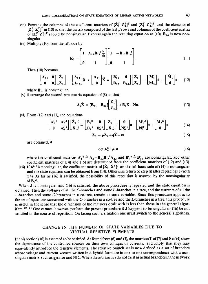
(iii) Permute the columns of the Coefficient matrices of [ZT illT and [ZT Z:lT, and the elements of [ZT ZT]’ in (10) so that the matrix composed of the last fl rows and columns of the coefficient matrix of [ZT ZZlT should be nonsingular. Express again the resulting equation as (10). B,, is now nonsingular.

(iv) Multiply (10) from the left side by

Then (10) becomes

where B; , is nonsingular. (v) Rearrange the second-row matrix equation of (8) so that

(vi) From (12) and (13), the equations

z, = pZ,+&+ril (15)

det Ail) # 0 (16)

are obtained, if

where the coefficient matrices AL’) 4 A - B 3 2 B- , ~ A , , and By) 9 B;, are nonsingular, and other coefficient matrices of (14) and (15) are determined from the coefficient matrices of (12) and (13).

(vii) If A:’) is nonsingular, the coefficient matrix of [ZT XTlT on the left-hand side of (14) is nonsingular and the state equation can be obtained from (14). Otherwise return to step (i) after replacing (8) with (14). As far as (16) is satisfied, the possibility of this repetition is assured by the nonsingularity of B:’).

When J is nonsingular and (1 6) is satisfied, the above procedure is repeated and the state equation is obtained. Then the voltages of all the C-branches and some L-branches in a tree, and the currents of all the L-branches and some C-branches in a co-tree, remain as state variables. Since this procedure applies to the set of equations concerned with the C-branches in a co-tree and the L-branches in a tree, this procedure is useful in the sense that the dimension of the matrices dealt with is less than those in the general algorithm.”-” One cannot, however, perform the present procedure if J happens to be singular or (16) be not satisfied in the course of repetition. On facing such a situation one must switch to the general algorithm.

CHANGE IN THE NUMBER OF STATE VARIABLES DUE T O VIRTUAL RESISTIVE ELEMENTS

In this section (16) is assumed to be satisfied. As found from (6) and (3), the matrices T of (7) and S of (4) show the dependence of the controlled sources on their own voltages or currents, and imply that they may equivalently introduce the resistive elements. The resistive branch set is now defined as a set of branches whose voltage and current vectors written in a hybrid form are in one-to-one correspondence with a nonsingular matrix, such as gyrator and NIC. When these branches do not exist as actual branches in the network

44 KOTARO HIRANO, FUMlAKI NISHI, AND SHIN-ICHIRO TOMIYAMA

N but are equivalently introduced, they are called virtual resistive elements and especially the virtual resistors when each of the voltages is controlled by its own current or each of the currents by its own voltage. In this section it is shown how the matrices T and S are related to the increase and the decrease in the number of state variables, respectively. Other kinds of virtual resistive elements due to the dependence of [JT, E;JT and [E:sv J:si]T on their own voltages or currents, can be considered. They do not, however, relate to the change in the number of state variables.

Increase case

For simplicity assume first that T = R& + GF,, where R& and Gyr are diagonal matrices, respectively, with the nonzero diagonal elements r;(k = 1,. . . , m) and gT( l = 1,. . . , n), where m and n are the number of C-branches in a co-tree and that of L-branches in the tree, respectively. Modify now the network N equivalently as follows, and denote the modified one by N;,,.

in S , with the R-branch rl composed of resistance r i and a controlled voltage source &,: , where El,,$ is given as the kth component of E,,r+ = [UEc R&]X

(ii) Replace the controlled current source .II.,, in rl with the R-branch g: composed of conductance is given as the Ith component of JI,g+ =

(iii) Introduce the Si-branches and &-branches with sensors alone in order to control E,.,+ and JI,g+, and denote them by S+ and S: , respectively.

(iv) Choose again the capacitor of S , and inductor of rl as a C-branch C: in the tree and an L-branch L: in the co-tree, respectively. Then, for them, choose r: and g: as a link and a tree branch, respectively.

In N:,,, the fundamental loops determined by virtual resistor r + contain only E, Si, C , and C+ and those determined by S: contain only E and C, and the fundamental cut-sets determined by virtual resistor g+ contain only J, S , , L, and L+ and those determined by S: contain only J and L. By eliminating unwanted variables from KVL, KCL, and branch voltage-current relations of N A , (8) in which Z = [I: V;]' is replaced with Z = [I,'+ v:+]', is obtained. Then multiplying (8) from the left side by the inverse of the coefficient matrix of [Z' x']' yields the state equation for N i d . This result is the same as that for N. Note that the vector [I,'+ V:+]' means [I$ V,']', and that the voltages and currents of other branches C, G, R, and L are identical with those for N. Thus the above consideration leads to the following conclusion. The C- branches S (in a co-tree of N) should be chosen as tree-branches in Ni, , , and the Lbranches r (in a tree of N) as links because of the existence of R-branches of the virtual resistors, and this causes the increase in the number of state variables.

The matrix T is not generally a diagonal one. Then. the resistive branch sets are virtually introduced and a similar argument also applies. These elements are treated just like resistors. Consider the case where T is singular. By applying the procedure in the Section 'Derivation of state equations', (8) is finally written in the forms of (14) and (15) in which source derivatives of high order appear. Then from (15), (6) can be rewritten

(i) Replace the controlled voltage source

+ [ V r RLIu.

[CY, H;LW + [GFr HT.1u. g: and a controlled current source JI ,g ,+ , where

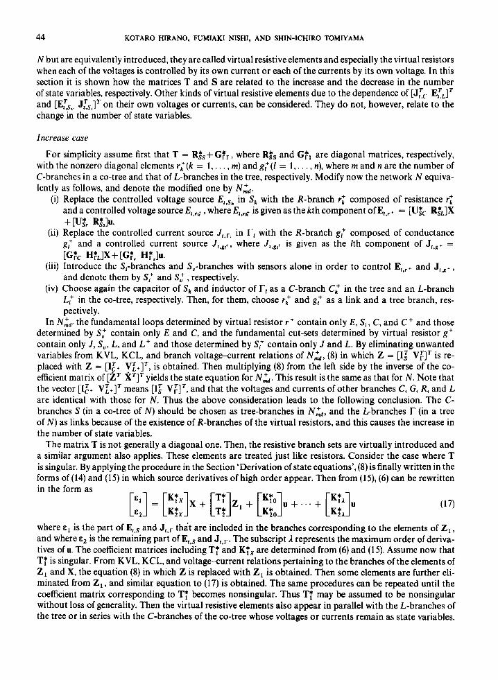
where E, is the part of E,,s and JI,r that are included in the branches corresponding to the elements of Z, , and where c2 is the remaining part of E,,s and Jf,r. The subscript I represents the maximum order of derivatives of u. The coefficient matrices including T: and KTx are determined from (6) and (15). Assume now that T: is singular. From KVL, KCL, and voltage-current relations pertaining to the branches of the elements of Z, and X, the equation (8) in which Z is replaced with Z, is obtained. Then some elements are further eli- minated from Z, , and similar equation to (17) is obtained. The same procedures can be repeated until the coefficient matrix corresponding to TT becomes nonsingular. Thus T: may be assumed to be nonsingular without loss of generality. Then the virtual resistive elements also appear in parallel with the L-branches of the tree or in series with the C-branches of the co-tree whose voltages or currents remain as state variables.


E t,R

%R

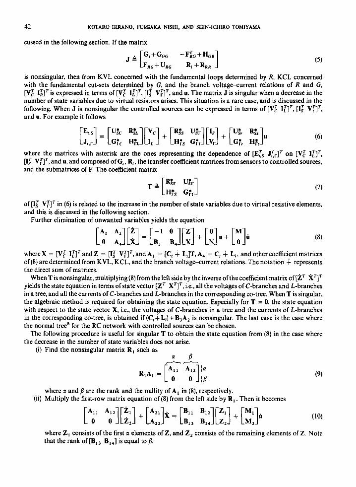
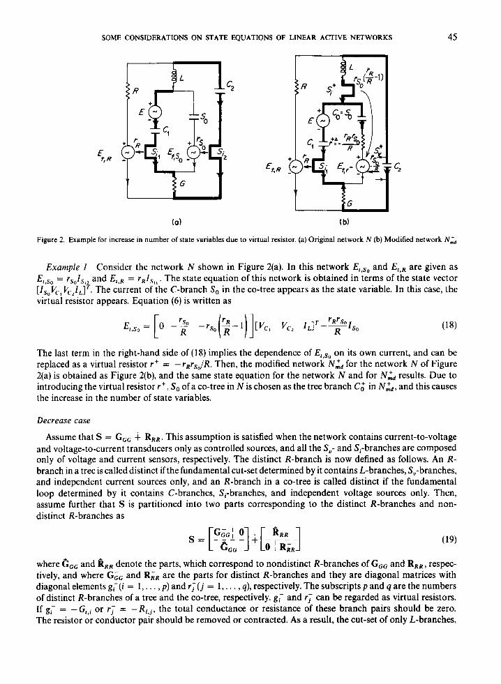
Figure 2. Example for increase in number of state variables due to virtual resistor. (a) Original network N (b) Modified network N:*

Example 1 Consider the network N shown in Figure 2(a). In this network and E f , R are given as = rsols,2 and Ef,R = r R I S , I . The state equation of this network is obtained in terms of the state vector

[IsoVcl VC2ILlT. The current of the C-branch So in the co-tree appears as the state variable. In this case, the virtual resistor appears. Equation (6) is written as

The last term in the right-hand side of (18) implies the dependence of on its own current, and can be replaced as a virtual resistor r + = - rRrsJR. Then, the modified network N:d for the network N of Figure 2(a) is obtained as Figure 2(b), and the same state equation for the network N and for N:,, results. Due to introducing the virtual resistor r', So of a co-tree in N is chosen as the tree branch C: in N:d, and this causes the increase in the number of state variables.

Decrease case

Assume that S = G,, i RRR. This assumption is satisfied when the network contains current-to-voltage and voltage-to-current transducers only as controlled sources, and all the So- and S,-branches are composed only of voltage and current sensors, respectively. The distinct R-branch is now defined as follows. An R- branch in a tree is called distinct if the fundamental cut-set determined by it contains L-branches, &-branches, and independent current sources only, and an R-branch in a co-tree is called distinct if the fundamental loop determined by it contains C-branches, Si-branches, and independent voltage sources only. Then, assume further that S is partitioned into two parts corresponding to the distinct R-branches and nondistinct R-branches as

where c,, and 8 R R denote the parts, which correspond to nondistinct R-branches of G G G and RRR , respectively, and where G;, and RRR are the parts for distinct R-branches and they are diagonal matrices with diagonal elements g;(i = 1,. . . , p ) and r ; ( j = 1,. . . , q), respectively. The subscripts p and q are the numbers of distinct R-branches of a tree and the co-tree, respectively. g; and r; can be regarded as virtual resistors. If g; = - Gt, , or r i = - Rltj, the total conductance or resistance of these branch pairs should be zero. The resistor or conductor pair should be removed or contracted. As a result, the cut-set of only L-branches,

46 KOTARO HIRANO, FUMUKI NISHI, AND SHIN-ICHIRO TOMIYAMA

&-branches, and independent current sources, or the loop of only C-branches, S,-branches, and independent voltage sources arises. This causes a decrease in the number of state variables.

Consider now the above argument more generally. By substituting (3) into the combination of (2-e) and (2-f) and then suitably permuting the coefficient matrices and the associated vectors including [I: Vi]', the branch voltage<urrent relation of R-branches can be rewritten as

where Q1 , is an n x n nonsingular matrix and any (n+ 1) x (n+ 1) submatrix obtained by adding the mth column and row, m > n, of the coefficient matrix of [q; qT3' to Q l l is singular, 5, = [I:, V,',]', 5, = [I,', V:JT, ql = [V,', I:,]', q2 = [V,', I:,]', and where $l and +2 are controlled sources expressed in terms of X, Z, and u. The branch sets G, and R, are composed of the elements of G and R corresponding to the columns of [Q,, Q,,], and G, and R2 are composed of remaining elements of G and R, respectively. From (20) g2 can be expressed in terms of kl, q,, $,, and 31, as 5, = Kt,S1 + K1,q2 + K*,(I~ + K#,Q2, where all the diagonal elements of K1, are equal to zero. That is, each current of G2 and each voltage of R2 can be expressed in terms independent of their own voltage and current, respectively, and thus G, and R, can be taken as controlled sources equivalently. In this case the resistors of G, and R, are cancelled by virtual resistors. While G, and R, can be taken as the resistive branch sets defined in the Section 'Change in number of state variables due to virtual resistive elements' with the branch voltage-current relation k1 = Qllqr + Q12q2 +JI1. Thus, G and R, remain as the resistive branch sets and G, and R, are replaced with controlled sources. It is needed to rechoose the tree and to rearrange the controlled sources and sensors when the modified network is constructed. Then, if some distinct R-branches are included in G, and R,, the decrease in the number of state variables arises because of the same reason as previously stated.

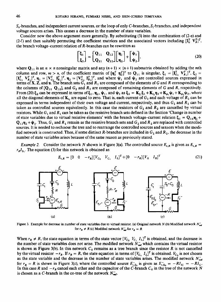
r R I S , . The equation (3) for this network is obtained as Example 2. Consider the network N shown in Figure 3(a). The controlled source E I , R is given as =

E t , R = [o 0 -rRl[VCo vC, -rRl[VG I d T (21)

E +n-

(a) (b) (C)

Figure 3. Example for decrease in number of state variables due to virtual resistor. (a) Original network N (b) Modified network Nid for rR # R (c) Modified network Nd for rR = R

When rR # R, the state equation in terms of the state vector [ V,, V,, I,]' is obtained, and the decrease in the number of state variables does not arise. The modified network N i d which contains the virtual resistor is shown in Figure 3(b). In this network Co remains as a tree branch since the resistor R is not cancelled by the virtual resistor -rR. If rR = R, the state equation in terms of [V,, ZLIT is obtained. V,, is not chosen as the state variable and the decrease in the number of state variables arises. The modified network Nmd for rR = R is shown in Figure 3(c), where the controlled source Els , is given as E,,, = -Rlsr = -RI,. In this case R and - rR cancel each other and the capacitor of the C-branch Co in the tree of the network N is chosen as a C-branch in the co-tree of the network Ns.


GENERAL ALGEBRAIC METHOD AND INITIAL VALUES

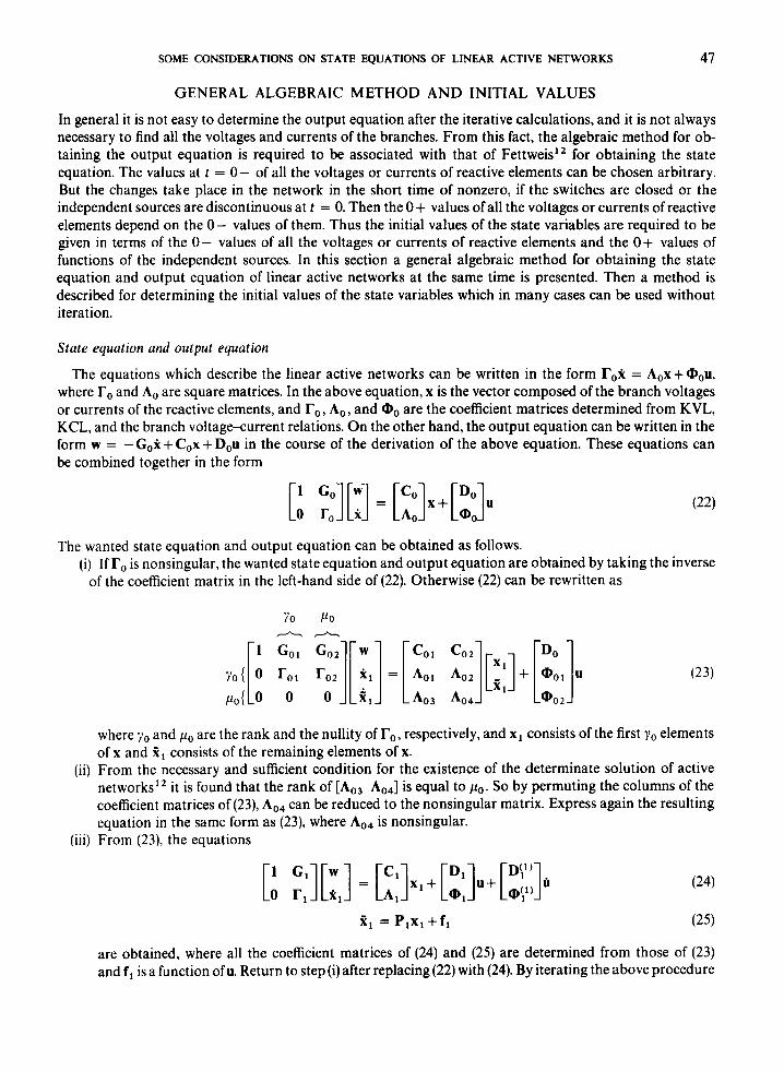
In general it is not easy to determine the output equation after the iterative calculations, and it is not always necessary to find all the voltages and currents of the branches. From this fact, the algebraic method for obtaining the output equation is required to be associated with that of Fettweis” for obtaining the state equation. The values at I = 0- of all the voltages or currents of reactive elements can be chosen arbitrary. But the changes take place in the network in the short time of nonzero, if the switches are closed or the independent sources are discontinuous at t = 0. Then the O+ values of all the voltages or currents of reactive elements depend on the 0- values of them. Thus the initial values of the state variables are required to be given in terms of the 0- values of all the voltages or currents of reactive elements and the O+ values of functions of the independent sources. In this section a general algebraic method for obtaining the state equation and output equation of linear active networks at the same time is presented. Then a method is described for determining the initial values of the state variables which in many cases can be used without iteration.

State equation and output equation

The equations which describe the linear active networks can be written in the form T0x = A0x+@,u, where To and A. are square matrices. In the above equation, x is the vector composed of the branch voltages or currents of the reactive elements, and To, A. , and Q0 are the coefficient matrices determined from KVL, KCL, and the branch voltagexurrent relations. On the other hand, the output equation can be written in the form w = -Gox+Cox+Dou in the course of the derivation of the above equation. These equations can be combined together in the form

The wanted state equation and output equation can be obtained as follows. (i) If To is nonsingular, the wanted state equation and output equation are obtained by taking the inverse

of the coefficient matrix in the left-hand side of (22). Otherwise (22) can be rewritten as

Yo Po nn

COl c 0 2

(23)

where y o and po are the rank and the nullity of To, respectively, and x1 consists of the first yo elements of x and 5 , consists of the remaining elements of x.

(ii) From the necessary and sufficient condition for the existence of the determinate solution of active networks” it is found that the rank of [Ao3 Ao4] is equal to p o . So by permuting the columns of the coefficient matrices of (23, A04 can be reduced to the nonsingular matrix. Express again the resulting equation in the same form as (23), where A04 is nonsingular.

(iii) From (23), the equations

jzl = P 1 x l + f l (25)

are obtained, where all the coefficient matrices of (24) and (25) are determined from those of (23) and f , is a function of u. Return to step (i) after replacing (22) with (24). By iterating the above procedure


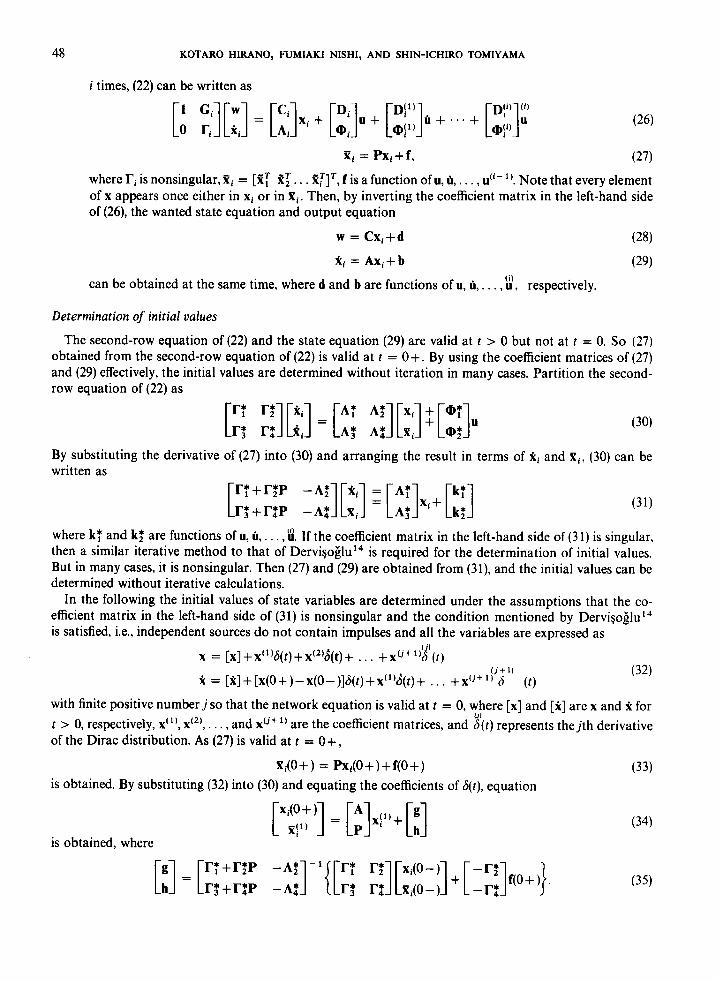
i times, (22) can be written as

z, = PXi+f, (27) where ri is nonsingular, Pi = [ZT 2;. . . %TIT, f is a function of u, 0,. . . , di- '). Note that every element of x appears once either in x i or in X i . Then, by inverting the coefficient matrix in the left-hand side of (26), the wanted state equation and output equation

w = C x i + d (28) xi = Axi + b (29)

(i) can be obtained at the same time, where d and b are functions of u, Q, . . . , u , respectively.

Determination of initial values

The second-row equation of (22) and the state equation (29) are valid at t > 0 but not at t = 0. So (27) obtained from the second-row equation of (22) is valid at t = O+. By using the coefficient matrices of (27) and (29) effectively, the initial values are determined without iteration in many cases. Partition the second- row equation of (22) as

By substituting the derivative of (27) into (30) and arranging the result in terms of x i and X i , (30) can be written as

where k: and k: are functions of u, 8, . . . , u. If the coefficient matrix in the left-hand side of (3 1) is singular, then a similar iterative method to that of Dervi~oHlu'~ is required for the determination of initial values. But in many cases, it is nonsingular. Then (27) and (29) are obtained from (31), and the initial values can be determined without iterative calculations.

In the following the initial values of state variables are determined under the assumptions that the coefficient matrix in the left-hand side of (31) is nonsingular and the condition mentioned by D e r v i ~ o i l u ' ~ is satisfied, i.e., independent sources do not contain impulses and all the variables are expressed as

I 7 x = [ X ] + X ( % ( t ) + X ( 2 ) 6 ( t ) + . . . + x ( J + " S ( t )

( j + 1 ) (32)

with finite positive number j so that the network equation is valid at t = 0, where [ x ] and [ x ] are x and x for t > 0, respectively, x ( ' ) , x('), . . . , and x(j+') are the coefficient matrices, and d(r) represents thejth derivative of the Dirac distribution. As (27) is valid at t = O+ ,

k = [ x ] + [ x ( O + ) - x ( O - ) ] 6 ( t ) + x ~ " ~ ( t ) + . . . + x ( J + ' ) s 0 )

01

X,(O+) = P x , ( O + ) + f ( O + ) (33) is obtained. By substituting (32) into (30) and equating the coefficients of &t), equation

is obtained, where


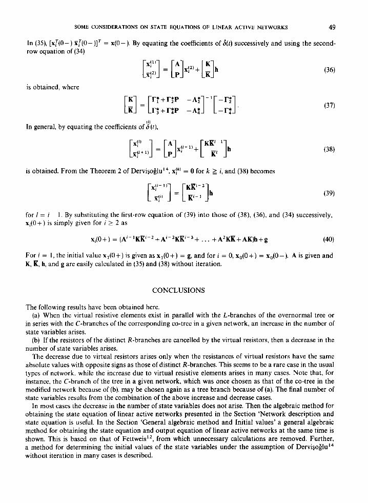
In (35), [xT(O-) jZT(O-)IT = x(0-). By equating the coefficients of 6(t) successively and using the second- row equation of (34)

is obtained, where

( 1 1 In general, by equating the coefficients of 6 ( t ) ,

is obtained. From the Theorem 2 of Dervi~oKlu'~, x!~) = 0 for k 2 i, and (38) becomes

for I = i - 1 . By substituting the first-row equation of (39) into those of (38), (36), and (34) successively, xi(O+) is simply given for i 2 2 as

xi(0+) = (Ai- 'KRi-2+Ai-2KRi-3+ ... +A2KR+AK)h+g (40)

For i = 1, the initial value x,(O+) is given as x,(O+) = g, and for i = 0, x,(O+) = x,(O-). A is given and K, R, h, and g are easily calculated in (35) and (38) without iteration.

CONCLUSIONS

The following results have been obtained here. (a) When the virtual resistive elements exist in parallel with the L-branches of the overnormal tree or

in series with the C-branches of the corresponding co-tree in a given network, an increase in the number of state variables arises.

(b) If the resistors of the distinct R-branches are cancelled by the virtual resistors, then a decrease in the number of state variables arises.

The decrease due to virtual resistors arises only when the resistances of virtual resistors have the same absolute values with opposite signs as those of distinct R-branches. This seems to be a rare case in the usual types of network, while the increase due to virtual resistive elements arises in many cases. Note that, for instance, the C-branch of the tree in a given network, which was once chosen as that of the co-tree in the modified network because of (b), may be chosen again as a tree branch because of (a). The final number of state variables results from the combination of the above increase and decrease cases.

In most cases the decrease in the number of state variables does not arise. Then the algebraic method for obtaining the state equation of linear active networks presented in the Section 'Network description and state equation is useful. In the Section 'General algebraic method and Initial values' a general algebraic method for obtaining the state equation and output equation of linear active networks at the same time is shown. This is based on that of Fettweis", from which unnecessary calculations are removed. Further, a method for determining the initial values of the state variables under the assumption of Derv i~oglu '~ without iteration in many cases is described.


REFERENCES

I . K. Hirano and S. Nishiniura, ‘Active RC filters containing periodically operated switches’, IEEE Trans. Circuit Theory. CT-19,

2. T. R. Bashkow, ‘The A matrix, new network description’, IRE Trans. Circuit Theory, CT-4, 117-120 (1957). 3. E. S. Kuh and R. A. Rohrer, ‘The state-variable approach to network analysis’, Proc. IEEE, 53,672-686 (1965). 4. K. Hirano and 1. Ogura, ‘Standard state equation form from a Lagrangian formulation’, Proc. IEEE(Letters), 58,498499 (1970). 5. K. Hirano and F. Nishi, ‘Mixed analysis of network with restriction on the branch partition’, Proc. 4th Asilomar Conf. Circuits

6. A. Dervi$o& ‘Bashkow’s “A matrix for active RLC networks” ’, IEEE Trans. Circuit Theory (Corresp.), CT-11,404-406 (1964). 7. N. DeClaris and R. Saeks, ‘Theoretic foundations of finite network and system analysis’, Aspects ofNetwork and System Theory,

8. K. Hirano, S. Nishimura, and S. Nakarnura, ‘State-variable approach to linear active RC networks’ (in Japanese), Monograph

9. E. J. Purslow, ‘Solvability and analysis of active networks by use of the state equations’, IEEE Trans. Circuit Theory, CT-17,

10. C. Pottle, ‘State space technique for general active network analysis’, System Anulysis by Digital Computers, F. K. Kuo and J. F.

11. E. Polak, ‘An algorithm for reducing a linear, time invariant differential system to state form’, IEEE Trans. Automatic Control

12. A. Fettweis, ‘On the algebraic derivation of the state equation’, IEEE Trans. Circuit Theory, CT-16, 171-175 (1969). 13. S. R. Parker and V. T. Barmes, ‘Existence of numerical solutions and the order of linear circuits with dependent sources’, IEEE

Trans. Circuit Theory, CT-18, 368-374 (1971). 14. A. DerviSoClu, ‘State equation and initial values in active RLC networks’, IEEE Trans. Circuit Theory (Corresp.), CT-18,544547

( 197 1). 15. K. Hirano and F. Nishi, ‘An algorithm for obtaining the state equation of linear RLC networks with controlled sources. (in

Japanese), Paper presented at the Joint Conference of the Kansai Sections of the Institutes related to Electrical Engineerings in Japan, G-200 October (1971).

253-260 (1972).

and Systems, Pacific Grove, Calif., 511-515 (1970).

N. DeCIaris and R. E. Kalman, Eds., Holt, New York, 1968.

of IECE, Japan, October (1970).

469475 (1970).

Kaiser, Eds, Wiley, New York, 1965.

(Short Papers), AC-11, 577-579 (1966).

16. J. Tow, ‘Order of complexity of linear active networks’, Proc. IEE, 115, 1259-1262 (1968). 17. S. Seshu and N. Balabanian, Linear Network Analysis, Wiley, New York, 1959.

Documents

Some considerations on state equations of linear active networks