Embed Size (px)
Citation preview
Petit retour sur le TD1
Some aspect concerning the LMDZ dynamical core and its use
1. GridStaggered grid and dynamics/physics interfaceZooming capabilityVertical discretizationNudging
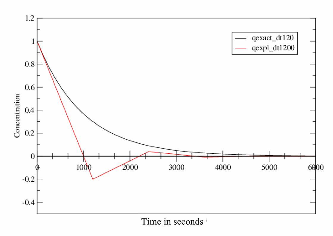
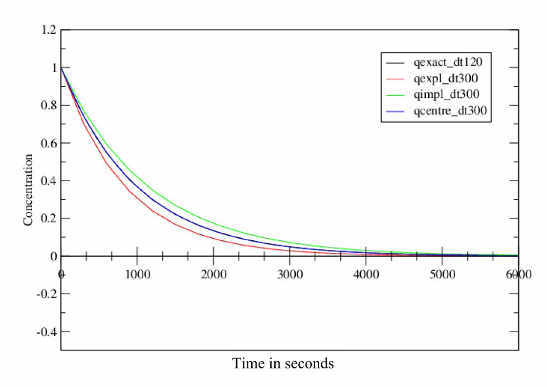
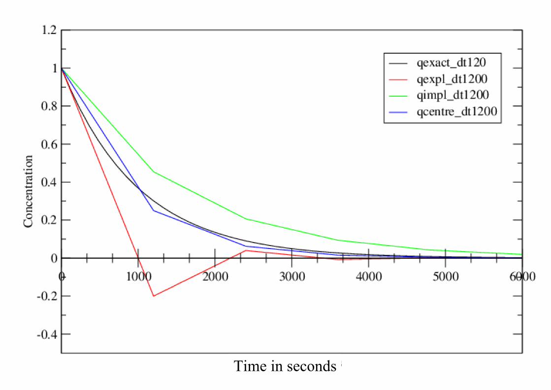
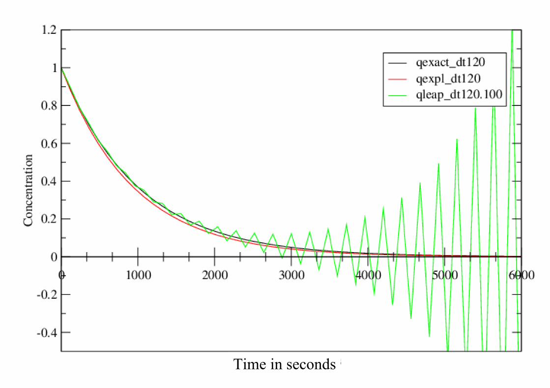
2. Temporal scheme and filteringTemporal schemes illustrated on a 0D modelThe Matsuno/Leapfrog schemeCFL criterion and longitudinal filtering
3. DissipationPrinciple of dissipation in 1DOperator splittingConstraints on the time step
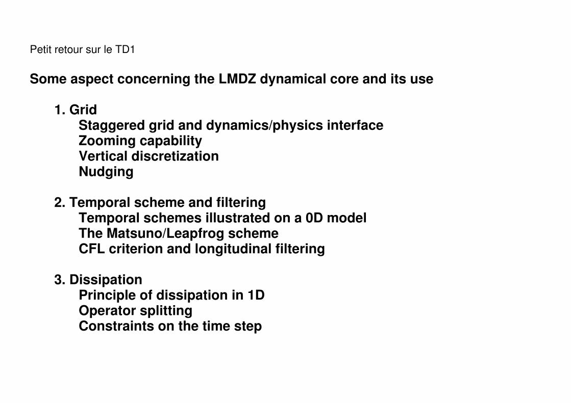
iim, jjm, llm
Defined atThe compilation
option-d 64x48x29In makegcmOr makelmdz*
http://lmdz.lmd.jussieu.fr/developpeurs/notes-techniques
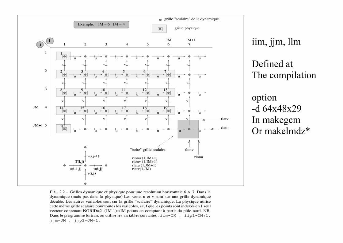
Zoom center :clon : longitude (degrees)clat : latitude (degrees)
grossimx/y : zooming factorin x/yComputed as the ration of theFinest model grid mesh length and of the equivalent length for the regular grid with same number of points.
dzoomx/y : fraction of the grid in which the resolution is increased.
clat
clon
dzomy *180°
dzomx * 360°δx=360° /iimδy=180°/jjm

http://lmdz.lmd.jussieu.fr/developpeurs/notes-techniques
Zoom center :clon : longitude (degrees)clat : latitude (degrees)
grossimx/y : zooming factorin x/yComputed as the ration of theFinest model grid mesh length and of the equivalent length for the regular grid with same number of points.
dzoomx/y : fraction of the grid in which the resolution is increased.
taux/y : « stiffness »
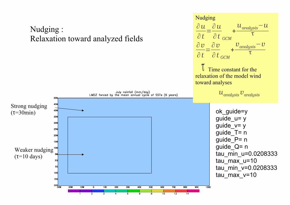
Strong nudging(τ=30min)
Weaker nudging(τ=10 days)
Nudging :Relaxation toward analyzed fields
ok_guide=yguide_u= yguide_v= yguide_T= nguide_P= nguide_Q= ntau_min_u=0.0208333tau_max_u=10tau_min_v=0.0208333tau_max_v=10
Nudging
Time constant for the relaxation of the model wind toward analyses
∂u∂ t
=∂u∂ t GCM
+u analysis−u
τ
∂v∂ t
=∂v∂ t GCM
+vanalysis−v
τ
τ
uanalysis vanalysis
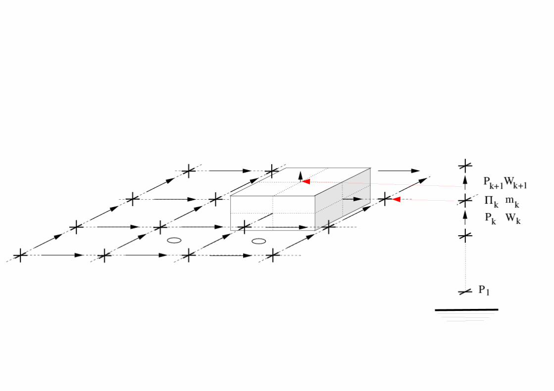
P 1 .....W 1=0
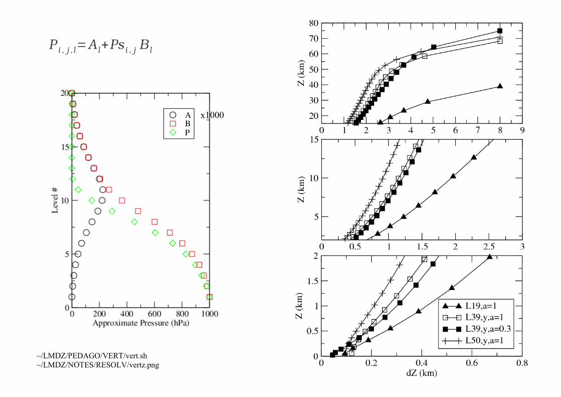
~/LMDZ/PEDAGO/VERT/vert.sh~/LMDZ/NOTES/RESOLV/vertz.png
x1000
P i , j , l=A l+Ps i , j B l
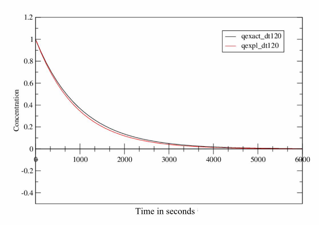
Time in seconds

Time in seconds
Time in seconds
Time in seconds
Time in seconds
Time in seconds

Contrôle du pas de temps dans gcm.def
day_step=960## periode pour le pas Matsuno (en pas)iperiod=5
Time in seconds
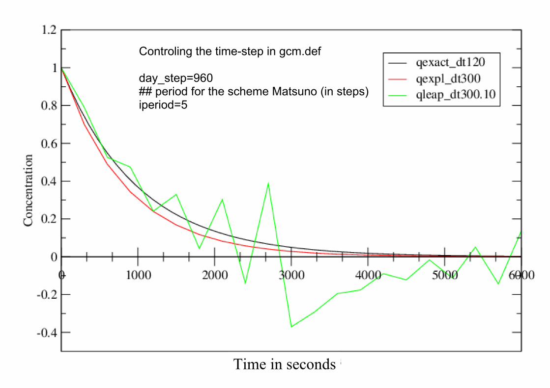
Controling the time-step in gcm.def
day_step=960## period for the scheme Matsuno (in steps)iperiod=5
Time in seconds
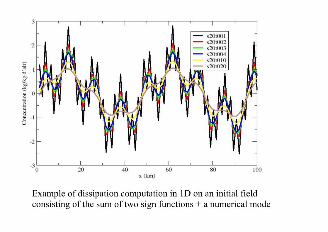
Example of dissipation computation in 1D on an initial fieldconsisting of the sum of two sign functions + a numerical mode
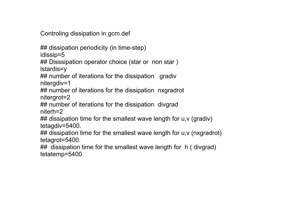
Controling dissipation in gcm.def
## dissipation periodicity (in time-step)idissip=5## Disssipation operator choice (star or non star )lstardis=y## number of iterations for the dissipation gradivnitergdiv=1## number of iterations for the dissipation nxgradrotnitergrot=2## number of iterations for the dissipation divgrad niterh=2## dissipation time for the smallest wave length for u,v (gradiv) tetagdiv=5400.## dissipation time for the smallest wave length for u,v (nxgradrot)tetagrot=5400.## dissipation time for the smallest wave length for h ( divgrad) tetatemp=5400.

Example of parameter tuning in gcm.defSensibility tests to horizontal resolution (Foujols et al.) http://forge.ipsl.jussieu.fr/igcmg/wiki/ResolutionIPSLCM4_v2
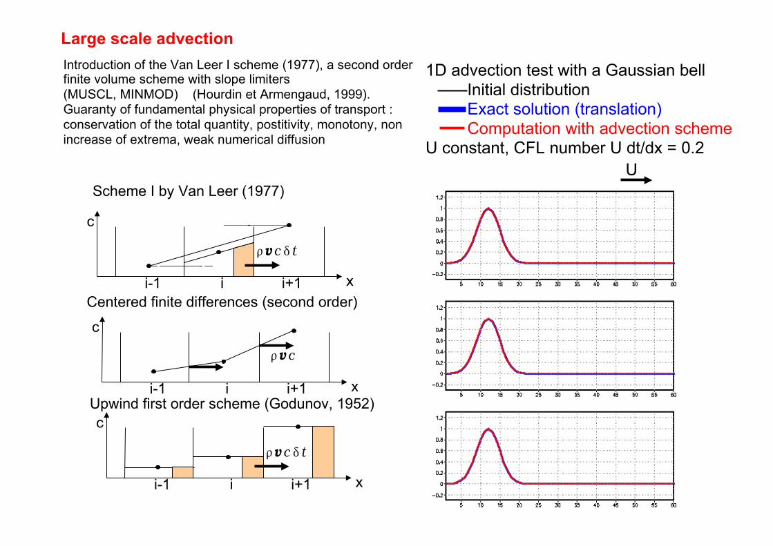
Large scale advection
1D advection test with a Gaussian bell Initial distribution Exact solution (translation) Computation with advection schemeU constant, CFL number U dt/dx = 0.2
Scheme I by Van Leer (1977)
x
c
v c t
Centered finite differences (second order)
x
c
v c
ii-1 i+1Upwind first order scheme (Godunov, 1952)
x
c
v c t
ii-1 i+1
ii-1 i+1
Introduction of the Van Leer I scheme (1977), a second order finite volume scheme with slope limiters(MUSCL, MINMOD) (Hourdin et Armengaud, 1999).Guaranty of fundamental physical properties of transport :conservation of the total quantity, postitivity, monotony, non increase of extrema, weak numerical diffusion
U
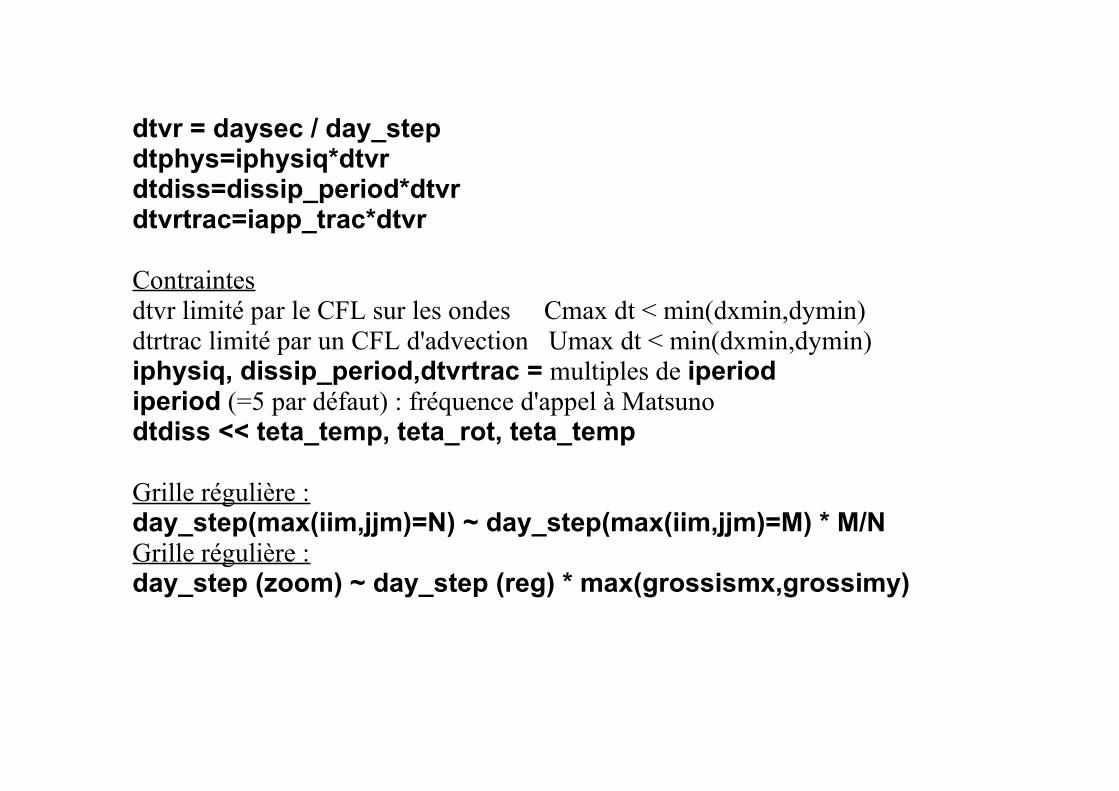
dtvr = daysec / day_stepdtphys=iphysiq*dtvrdtdiss=dissip_period*dtvrdtvrtrac=iapp_trac*dtvr
Contraintesdtvr limité par le CFL sur les ondes Cmax dt < min(dxmin,dymin)dtrtrac limité par un CFL d'advection Umax dt < min(dxmin,dymin) iphysiq, dissip_period,dtvrtrac = multiples de iperiodiperiod (=5 par défaut) : fréquence d'appel à Matsunodtdiss << teta_temp, teta_rot, teta_temp
Grille régulière :day_step(max(iim,jjm)=N) ~ day_step(max(iim,jjm)=M) * M/NGrille régulière :day_step (zoom) ~ day_step (reg) * max(grossismx,grossimy)

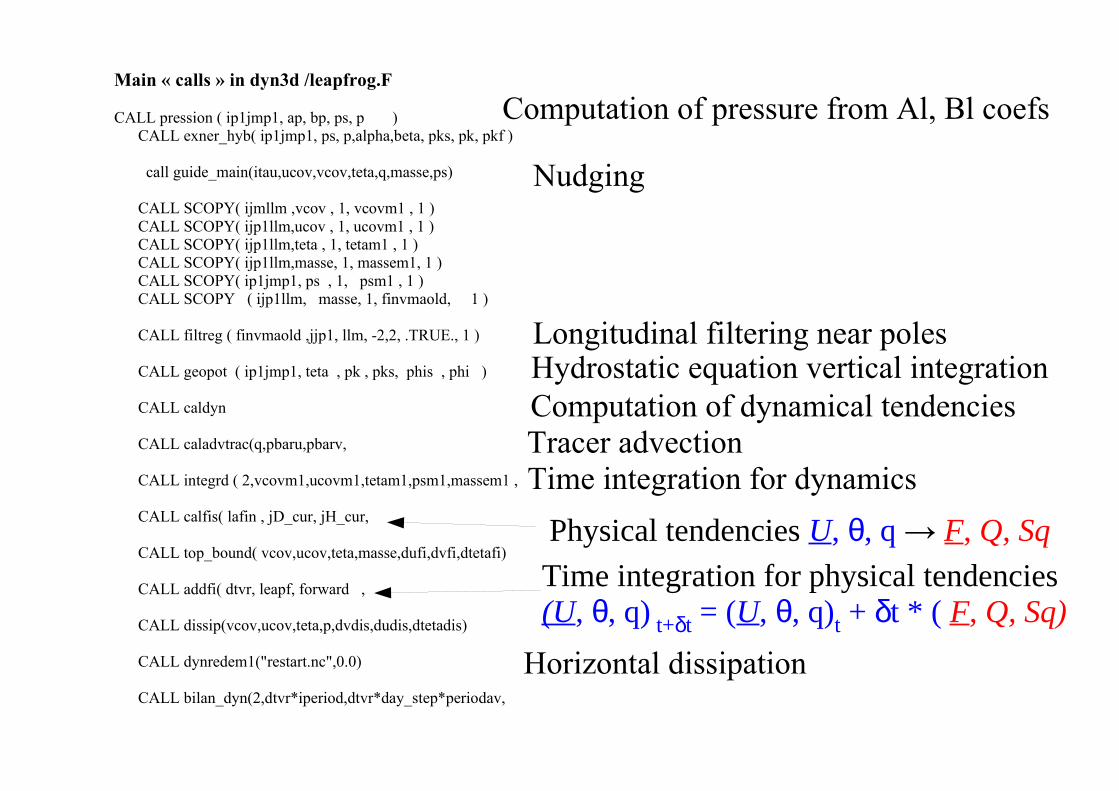
Main « calls » in dyn3d /leapfrog.F CALL pression ( ip1jmp1, ap, bp, ps, p ) CALL exner_hyb( ip1jmp1, ps, p,alpha,beta, pks, pk, pkf )
call guide_main(itau,ucov,vcov,teta,q,masse,ps)
CALL SCOPY( ijmllm ,vcov , 1, vcovm1 , 1 ) CALL SCOPY( ijp1llm,ucov , 1, ucovm1 , 1 ) CALL SCOPY( ijp1llm,teta , 1, tetam1 , 1 ) CALL SCOPY( ijp1llm,masse, 1, massem1, 1 ) CALL SCOPY( ip1jmp1, ps , 1, psm1 , 1 ) CALL SCOPY ( ijp1llm, masse, 1, finvmaold, 1 )
CALL filtreg ( finvmaold ,jjp1, llm, -2,2, .TRUE., 1 )
CALL geopot ( ip1jmp1, teta , pk , pks, phis , phi )
CALL caldyn
CALL caladvtrac(q,pbaru,pbarv,
CALL integrd ( 2,vcovm1,ucovm1,tetam1,psm1,massem1 ,
CALL calfis( lafin , jD_cur, jH_cur,
CALL top_bound( vcov,ucov,teta,masse,dufi,dvfi,dtetafi)
CALL addfi( dtvr, leapf, forward ,
CALL dissip(vcov,ucov,teta,p,dvdis,dudis,dtetadis)
CALL dynredem1("restart.nc",0.0)
CALL bilan_dyn(2,dtvr*iperiod,dtvr*day_step*periodav,
Physical tendencies U, θ, q → F, Q, Sq
Time integration for physical tendencies (U, θ, q) t+δt = (U, θ, q)t + δt * ( F, Q, Sq)
Computation of dynamical tendenciesTracer advectionTime integration for dynamics
Horizontal dissipation
Longitudinal filtering near poles
Nudging
Computation of pressure from Al, Bl coefs
Hydrostatic equation vertical integration