SOMBRERO USer Manual - Censolar - CENSOLAR (Centro de Estudios de

Universität-GesamthochschuleSiegen

FG Bauphysik & SolarenergieLtg.: Prof. Dr.-Ing. F.D. Heidt

Gefördert durch:

SOMBRERO(VERSION 3.0)

A PC-TOOL TO CALCULATE SHADOWS ON

ARBITRARILY ORIENTED SURFACES

Group for Building Physics & Solar Energy (Head: Prof. Dr.-Ing. F.D. Heidt)

University of Siegen D-57068 Siegen

Germany

AG SOLARNORDRHEIN-WESTFALEN

Universität-GesamthochschuleSiegen

FG Bauphysik & SolarenergieLtg.: Prof. Dr.-Ing. F.D. Heidt

Gefördert durch:

SOMBRERO(VERSION 3.0)

A PC-TOOL TO CALCULATE SHADOWS ON

ARBITRARILY ORIENTED SURFACES

User Manual

Development:

Dipl.-Phys. A. Eicker, Dipl.-Phys. A. Niewienda,

Dipl.-Phys. J. Clemens

Contact Address and Copyright:

Group for Building Physics and Solar Energy Head: Prof. Dr.-Ing. F.D. Heidt

University of Siegen D-57068 Siegen

Germany

AG SOLARNORDRHEIN-WESTFALEN

SOMBRERO 3.0 User Manual 5

SOMBRERO 3.0

User Manual - Contents

1 Introduction . . . . . . . . . . . . . . . . . . . . . . . . . . . . 7

2 Installation . . . . . . . . . . . . . . . . . . . . . . . . . . . . . 7

2.1 System requirements . . . . . . . . . . . . . . . . . . . . . . . . 7

2.2 Installation of the program . . . . . . . . . . . . . . . . . . . . . . 8

2.3 De-installation of the program . . . . . . . . . . . . . . . . . . . . . 8

2.4 VRML player . . . . . . . . . . . . . . . . . . . . . . . . . . . 8

3 Using the program . . . . . . . . . . . . . . . . . . . . . . . . . . 9

4 Data file generator . . . . . . . . . . . . . . . . . . . . . . . . . . 9

4.1 Co-ordinate systems and angles . . . . . . . . . . . . . . . . . . . . 9

4.2 The "surface of earth"-system . . . . . . . . . . . . . . . . . . . . . 10

4.3 The u-v system . . . . . . . . . . . . . . . . . . . . . . . . . . 10

4.4 Name of the data file . . . . . . . . . . . . . . . . . . . . . . . . 11

4.5 Comment lines . . . . . . . . . . . . . . . . . . . . . . . . . . 11

4.6 Input of objects . . . . . . . . . . . . . . . . . . . . . . . . . . 12

4.7 Generating houses . . . . . . . . . . . . . . . . . . . . . . . . . 14

4.8 Generating trees . . . . . . . . . . . . . . . . . . . . . . . . . . 16

4.9 Opening of an existing data file . . . . . . . . . . . . . . . . . . . . 17

4.10 Creating a new data file on the basis of an opened project . . . . . . . . . . 17

4.11 Editing an existing data file . . . . . . . . . . . . . . . . . . . . . . 17

4.12 Horizontal shading . . . . . . . . . . . . . . . . . . . . . . . . . 17

5 Adjusting the parameters for the simulation . . . . . . . . . . . . . . . 18

5.1 Parameter page 1 . . . . . . . . . . . . . . . . . . . . . . . . . 18

5.2 Parameter page 2 . . . . . . . . . . . . . . . . . . . . . . . . . 20

6 Output data . . . . . . . . . . . . . . . . . . . . . . . . . . . . 21

6.1 Mean-value file (*.MIT) . . . . . . . . . . . . . . . . . . . . . . . 21

6.2 Report file (*.REP) . . . . . . . . . . . . . . . . . . . . . . . . . 22

6.3 VRML file (*.WRL) . . . . . . . . . . . . . . . . . . . . . . . . . 22

6.4 Export format . . . . . . . . . . . . . . . . . . . . . . . . . . . 22

7 Ground reflection . . . . . . . . . . . . . . . . . . . . . . . . . . 23

8 Simulation . . . . . . . . . . . . . . . . . . . . . . . . . . . . . 24

8.1 Name of output files . . . . . . . . . . . . . . . . . . . . . . . . 24

8.2 Start simulation . . . . . . . . . . . . . . . . . . . . . . . . . . 24

6 Benutzungshandbuch SOMBRERO 3.0

9 Example for the use of the data file generator . . . . . . . . . . . . . . 24

9.1 Creating the data file . . . . . . . . . . . . . . . . . . . . . . . . 25

9.2 Generating the rectangular collector face . . . . . . . . . . . . . . . . 25

9.3 Generating the shadow throwing house . . . . . . . . . . . . . . . . . 26

9.4 Finishing the data file generator . . . . . . . . . . . . . . . . . . . . 28

9.5 VRML view of the project data . . . . . . . . . . . . . . . . . . . . . 29

10 Calculating the diffuse radiation with SOMBRERO . . . . . . . . . . . . . 29

10.1 Motivation . . . . . . . . . . . . . . . . . . . . . . . . . . . . 29

10.2 Geometric model . . . . . . . . . . . . . . . . . . . . . . . . . . 30

10.3 Weighting factors . . . . . . . . . . . . . . . . . . . . . . . . . 31

10.4 Determination with the projection algorithm . . . . . . . . . . . . . . . . 32

11 Limited liability . . . . . . . . . . . . . . . . . . . . . . . . . . . 32

12 Comments / suggestions . . . . . . . . . . . . . . . . . . . . . . . 33


1 Introduction For both active use of solar energy (domestic hot water, photovoltaic) as well as for passive solar architecture, shading or lighting of planes plays an important role. SOMBRERO calculates quantitative results for shading of collectors or windows by buildings, trees, overhangs or the horizon. After an idea of J. A. Clark an algorithm has been developed which allows to project three-dimensional objects, which are characterized through their surfaces, in the plane of a collector or window. This projection is a function of the position of the sun depending on the day of the year, the time, the time zone and the geographical latitude and longitude. Three-dimensional objects are built up by their boundary planes. Objects like houses and trees are predefined and described by parameters like height, width and position in space. Single planes are described by their vertex points in the two-dimensional co-ordinate system related to the plane itself (in case of rectangles simply by their length and height) and positioned by indication of azimuth, elevation and origin in the three-dimensional space. We wish you a pleasant work with the program and many valuable results. Your SOMBRERO Team Head: Prof. Dr.-Ing. F.D. Heidt Autors: Dipl.-Phys. A. Eicker Dipl.-Phys. A. Niewienda Dipl.-Phys. J. Clemens

2 Installation

2.1 System requirements Minimal system requirements

The minimal system requirements for the work with SOMBRERO are:

• PC (486DX or better);

• about 5 MB of free space on your hard disc;

• Windows 95 / NT;

• graphics board with resolution 800 x 600.


2.2 Installation of the program For the install of the program do the following: Installation form a disc: • Insert your SOMBRERO installation disc into your drive;

• Open in the "Explorer" or "Work Place" drive A: (Windows 95, 98 or NT);

• Start the install program "Setup";

• Follow the instructions of the install program. Installation of the downloads from the Internet: • Start the install program "SOMBRERO_Setup";

• Follow the instructions of the install program.

2.3 De-installation of the program For the de-installation of the program do the following: • Open the system control (Start - Adjustments - system control);

• Open the file "Software";

• Choose "SOMBRERO" in the list of programs and click on "remove";

• Follow the instruction of the de-installation program.

2.4 VRML-Player For the three-dimensional view of the VRML file created by SOMBRERO (see Chapter 6.3) you need a VRML player. This can be a program or a plug-in of an internet browser. If a VRML player is already installed on your system, SOMBRERO will find it automatically. Is there no VRML player on your system, you can download a lot of them from the internet for free. SOMBRERO has been tested with the following VRML players:

• Cosmoplayer (Version 2.1) Plug-In for Netscape Navigator and Internet Explorer, Download: 'http://www.cosmosoftware.com'

• GLView (Version 4.4) Program, Download: 'http://www.glview.com'

• Blaxxun (Version 4.3) Plug-In for Netscape Navigator and Internet Explorer, Download: 'http://www.blaxxun.com'

• Cortona (Version 2.2) Plug-In for Netscape Navigator and Internet Explorer, Download: 'http://'www.parallelgraphics.de'


In case an executable VRML player is installed on your system and SOMBRERO does not find it, or you want to use another one as the standard player, you can specify the name of the program (including drive and program path) in SOMBRERO in "Options - VRML Viewer - Other Browser"

3 Using the program You may start SOMBRERO like any other Windows application. The program can be controlled by mouse or keyboard. All common shortcuts are available. The program only needs the input of text and numeric variables. The introductory screen disappears when you click the "OK" - button (or simply hit the <RETURN> - key). Now you are in the main menu of SOMBRERO. From here you can do all the inputs the program needs for calculation and simulation.

4 Data file generator The date file generator offers a convenient preparation of a description of the geometrical conditions for a shadow throw simulation with SOMBRERO. Planes can be defined as any polygons. At target planes, the possibility exists to generate overhangs at any side. All target faces must be situated in one plane, the target plane. In addition, you may enter standard houses as shadow generating objects. These houses have a rectangular base and a symmetrical gabled roof. Furthermore, you may define trees through information of height, diameter of the trunk, and diameter of the crown. Hereby the different foliage of the tree in the course of the year can be controlled optionally by entering a monthly schedule. The total number of planes is limited to 200, where for the generation of a standard house or a tree 7 faces are required.

4.1 System of co-ordinates and angles For the definition of planes, two systems of co-ordinates and two angles are required. These should be illustrated by means of the following example: The shading of two windows which face southeast should be examined. The shading is caused by a second house lying to the southeast. From the present floor plan (supervision), the size and alignment of the houses and the relative position to each other can be taken (Fig. 1). The shaded house wall with the two windows is drawn in bold face. The size and position of the two windows can be taken from the corresponding elevation, e.g. "view south“ (Fig. 2). These two plans are represented schematically here, where the used co-ordinate systems are shown. The user is free to select the origin and is able to select it such as the description of the geometry becomes as simple as possible.


11

5

0 2 5 7 9

20

5

-45

Fig. 1: Floor plan of the two houses (supervision) Fig. 2: View of the shaded house wall.

4.2 The 'surface on earth'-system (SOE) First of all a stationary, dextral, Cartesian co-ordinate system with the axes x, y and z is introduced to describe the 3-dimensional space. In this 'surface on earth'-system (SOE), the y-axis is pointing north and the z-axis to the sky. The x-axis points east. The origin of the system can be determined by the user. It is reasonable to set the origin onto an edge of an object and to select z = 0 as the upper plane of the bottom plane, so that z indicates the height over the bottom plane. Our system is drawn in into the floor plan. The z-axis points upwards and z = 0 lies at height of the bottom plane.

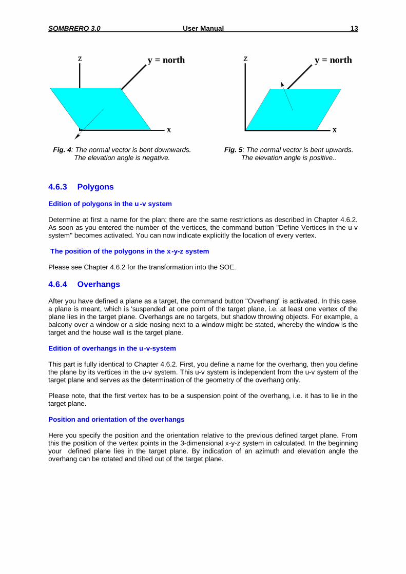
4.3 The u-v system For the description of target planes a 2-dimensional, Cartesian co-ordinate system with the axes u and v is introduced. The u-v system is a co-ordinate system related to the plane itself. It forms a plane which contains the surface that has to be described. All polygons which lie in this plane are defined by specification of the co-ordinates (u,v) of their vertices. To describe the two windows (targets), first of all the target plane has to be defined through an object-related u-v co-ordinate system. The target plane in Fig. 1 is a southeast wall and the origin of the u-v system is for logical reasons set into the lower left corner (Fig. 2). Now the situation and geometry of the two windows can easily be defined through specification of the co-ordinates (u,v) of its vertices. Finally, the position and orientation of the target plane has to be determined in the SOE. The adjustment of a plane is fixed by its azimuth- and elevation angles. The azimuth indicates the orientation of the perpendicular vector of the target plane as projected into the x-y-plane of SOE. An azimuth of 0° means, that this normal vector at the surface points north. The azimuth can range between 0° and 360° and is clockwise counted (Fig. 3). The elevation indicates the inclination of the plane against the x-z plane of the SOE. An elevation of 0° means a ‘vertical wall’ (parallel to the x-z plane). The elevation can range between -90° and +90°. Here, positive and negative angles are corresponding to a normal vector pointing upwards and downwards, respectively (see Fig. 4 and Fig. 5). The position of the target plane in the 3-dimensional SOE is determined by the choice of the origin (u0,v0) of the u-v system within the x-y-z system.


ε = 30°

α = 180°

z

x

y = North

n

v

u

Fig. 3: This figure shows the connection between SOE and u-v system. In addition, the angles

α (azimuth) and ε (elevation) are drawn in, to define the relative orientation of the two systems. The position of a plane in the SOE is described through a point (u0,v0) and the direction of the normal vector n̂ .The normal points outwards, i.e. from a facade in the direction of the environment. The point (u0,v0) represents the left, lower corner of the plane if the observer looks at the facade from the outside. So in natural manner the utilization of the floor plan and the elevation is possible for

the description of the geometry

4.4 Name of the data file With the button "New Basis Project" a new data file can be created. At first the name of the data file which has to be produced must be entered into a dialog box. Also the path where the file is saved is indicated here. The pre-defined adjustment is the sub-directory "Data" of the directory chosen at the installation. Should another directory be used as standard, you can change the pre-defined directory at "Options - Userdirectory". The name of the project is shown in the title bar of the main form constantly. All changes of the data file are saved automatically; an explicit saving of the data is not necessary.

4.5 Comment lines By clicking the button "Enter Comment“ you can enter as many comment lines as you like, which describe the data file. These comment lines are added to the beginning of the data file and are marked with an ‘*’ as the first sign.The ‘*’ will be set to the beginning of a comment line automatically by SOMBRERO. These lines will be ignored by SOMBRERO. Clicking on the "OK"-button terminates this function.


4.6 Input of objects 4.6.1 Targets To start a calculation with SOMBRERO at least one target must be defined. All target areas must be in one plane. This target plane is described through a Cartesian u-v co-ordinate system related to the plane itself. So through specification of the co-ordinates (u,v) a point in the target plane is determined. You can define rectangles or polygons with n vertices as target planes, when you activate the check box "Target plane" in the form of the corresponding plane. At the input of targets it is important to enter the planes in such a way, as if the observer looks from the outside onto the planes (like in Fig. 3). In this way the planes are usually represented in the elevation plan. Subsequent the position and the alignment of the target level is determined in the 3-dimensional x-y-z system which is fixed in space. Finally, you can generate overhangs with any alignment at any positions of the target plane, which are transformed automatically during displacement or turns of the target plane. 4.6.2 Rectangles Edition of rectangles in the u-v system You first indicate the denotation of the plane. You can employ any name with up to 80 characters here. The only restriction is, that the name should not start with ‘baum’ , ‘stamm’ or 'frontseite', because these phrases are reserved for the generation of trees and houses. Please enter now the length of the edge in u- and v-direction and the co-ordinates of the lower left vertex. Position in SOE-system Here you enter the necessary information for the position and direction of the target plane into the 3-dimensional x-y-z system. The following information is required in detail: • Azimuth of the plane:

You can enter an angle between 0° and 360°. Hereby 0° means a northern plane, the values are counted clockwise. So 90° means an eastern plane and 270° a western plane (Fig 3).

• Elevation of the plane:

Here you can enter a value from -90° to 90° for the angle between the normal vector (perpendicular to the plane) and the horizontal. If the normal vector points upwards, the angle is counted positively; at normal vector tilting down, the angle is counted negatively. So consequently 0° means a vertical plane, 90° a horizontal plane with a normal vector upwards and 90° a horizontal plane with a normal vector down (see Fig. 4 and 5). Annotation: It is unimportant for a horizontal overhang, whether the elevation amounts +90° or -90°.

• Position of the origin:

Here you determine the position (x,y,z) in the 3-dimensional space where the origin of your plane (u0, v0) should be set.


y = north y = north

Fig. 4: The normal vector is bent downwards.

The elevation angle is negative.

Fig. 5: The normal vector is bent upwards. The elevation angle is positive..

4.6.3 Polygons Edition of polygons in the u -v system Determine at first a name for the plan; there are the same restrictions as described in Chapter 4.6.2. As soon as you entered the number of the vertices, the command button "Define Vertices in the u-v system" becomes activated. You can now indicate explicitly the location of every vertex. The position of the polygons in the x-y-z system Please see Chapter 4.6.2 for the transformation into the SOE. 4.6.4 Overhangs After you have defined a plane as a target, the command button "Overhang" is activated. In this case, a plane is meant, which is 'suspended' at one point of the target plane, i.e. at least one vertex of the plane lies in the target plane. Overhangs are no targets, but shadow throwing objects. For example, a balcony over a window or a side nosing next to a window might be stated, whereby the window is the target and the house wall is the target plane. Edition of overhangs in the u-v-system This part is fully identical to Chapter 4.6.2. First, you define a name for the overhang, then you define the plane by its vertices in the u-v system. This u-v system is independent from the u-v system of the target plane and serves as the determination of the geometry of the overhang only. Please note, that the first vertex has to be a suspension point of the overhang, i.e. it has to lie in the target plane. Position and orientation of the overhangs Here you specify the position and the orientation relative to the previous defined target plane. From this the position of the vertex points in the 3-dimensional x-y-z system in calculated. In the beginning your defined plane lies in the target plane. By indication of an azimuth and elevation angle the overhang can be rotated and tilted out of the target plane.


• Lateral building (wing wall):

The plane is rotated by a relative azimuth angle between 0° and 180° around the v - axis out of the target plane. Subsequently the suspension point ( 0u = , 0v = ) is moved to the wanted position in the target plane (Fig. 6 to 8).

Fig. 6: The geometry of the plane is

defined in the u-v system. Fig. 7: The plane is rotated by 90°

around the v - axis out of the target plane.

Fig. 8: The suspension point is moved into the target plane.

• Overhang:

The plane is now tilted by a negative elevation angle between 0° and -180° around the u - axis out of the target plane. The angle is counted negatively, because the normal vector of the plane is bent downwards (see Fig 4). Afterwards the suspension point ( 0u = , 0v = ) is moved to the wanted position in the target plane (Fig. 9 to Fig.11).

Fig. 9: The geometry of the plane is determinated in the u-v system.

Fig. 10: The plane is tilted by -90° around the u-axis out of the

target plane.

Fig. 11: The suspension point is moved into the target plane.

When all inputs are made correctly, please use the "OK"-button to finish the generation of the overhang.

4.7 Generating houses 4.7.1 General With this menu item, you can generate a single house with rectangular basis and a gabled roof. The house is represented by 7 planes (4 side walls, 2 roof planes, 1 gable plane). At first the dimensions of the house are determined and then the position in the x-y-z system is specified. In SOMBRERO, houses can not be defined as targets, but exclusively as shadow throwing objects.


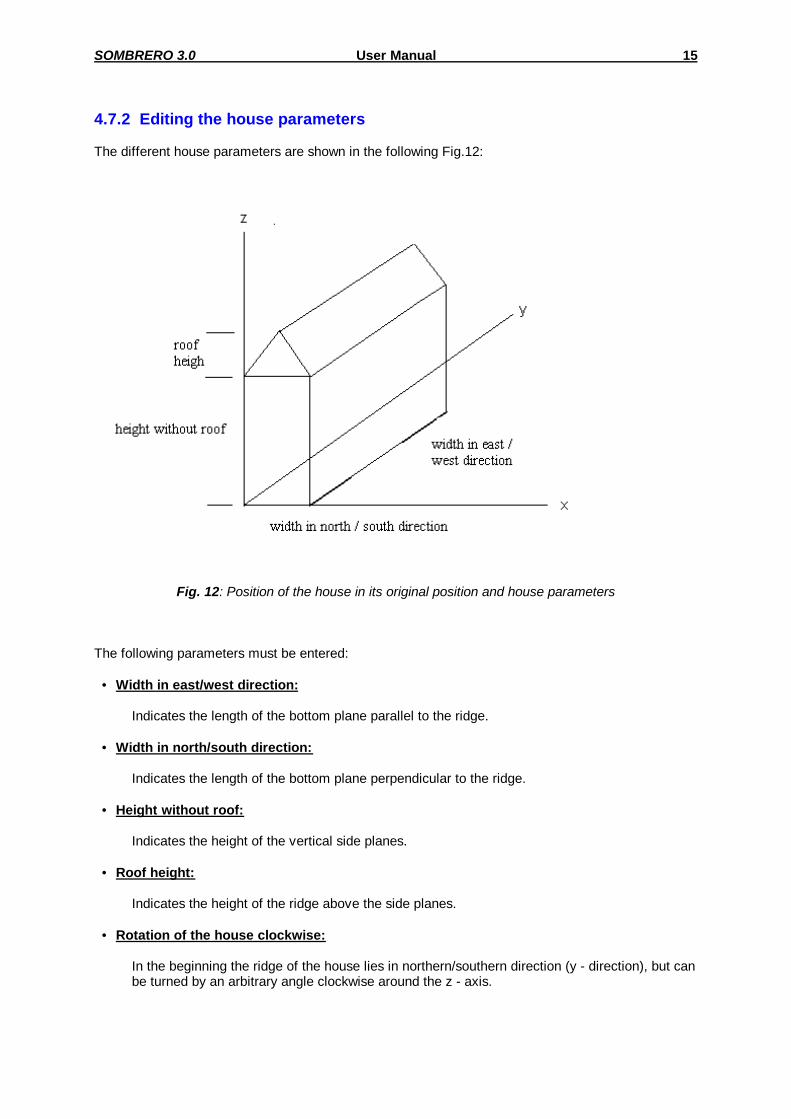
4.7.2 Editing the house parameters The different house parameters are shown in the following Fig.12:

Fig. 12: Position of the house in its original position and house parameters

The following parameters must be entered: • Width in east/west direction:

Indicates the length of the bottom plane parallel to the ridge. • Width in north/south direction:

Indicates the length of the bottom plane perpendicular to the ridge. • Height without roof:

Indicates the height of the vertical side planes.

• Roof height:

Indicates the height of the ridge above the side planes.

• Rotation of the house clockwise:

In the beginning the ridge of the house lies in northern/southern direction (y - direction), but can be turned by an arbitrary angle clockwise around the z - axis.


• Translation by vector:

Before the rotation the house is located in the first quadrant with positive co-ordinates x and y. The bottom plane lies at z = 0. Now you can move the house to the wanted position in the x-y-z system after the rotation by indicating a shifting vector.

Annotation: The transformations in the x-y-z system are not commutative. First the rotation

(around the z-axis) and then the shifting occurs.

By clicking the "OK"-button you can leave the menu. The 7 planes of the house are written into the data file and you are back in the ‘Generating Objects’ - menu. For further information see the example in Chapter 9.

4.8 Generating trees 4.8.1 General With this menu point you are able to generate a deciduous tree which consists of a rectangular trunk and a globular crown. The rectangular trunk is represented by 3 side planes. The shadow of the fourth side plane is in any case covered by the shadows of the three other planes, so we can forget this one. The globular crown is represented by 3 vertical standing octagons and one horizontal lying octagon. The vertical octagons are inclined 60° to each other, and two of them cut each other in a line. The horizontal octagon cuts the others in the middle. Altogether 7 planes are needed for the representation of a tree. In order to consider the variable foliage of different trees in the course of a year, you can enter for every month a factor between 0% and 100% for the shadow throwing of the tree. A factor of 60% causes, for example, that the shading of a half by the tree will be indicated with 30% ( )5.06.0 ×= instead of 50%. 4.8.2 Editing the tree parameters In this form you can enter the following tree parameters: • Height of the trunk

Designates the length of the trunk measured from the foot of the tree up to the lower edge of the tree top.

• Diameter of the trunk

Designates the width of the 3 vertical rectangles which represent the trunk. • Diameter of the tree top

Designates the distance between two facing sides of the octagons which represent the tree top.


• Foliage schedule

The priority factors of the foliage can be defined here for the different months. This data can also be saved into and loaded from an extern file. To change the schedule, please click onto the command button "Change Foliage". After all parameters are entered correctly, you can leave this point by clicking the "OK"-Button. The generated tree will be saved into the date file and you are back to the object selection menu. The number of the trees is only limited by the maximum total number of the planes (= 200).

4.9 Opening an existing data file Open an existing data file by pressing the button "Open Project".

4.10 Creating a new data file on the basis of an opened project Use the Button "New Variation of the Project" to open a new project in which the data of the opened file is added automatically. The original data file will remain unchanged.

4.11 Editing an open data file By clicking the button "Edit Object Data" in the main form you are able to insert, edit or delete any elements of the opened project. Under special circumstances it is easier to delete an existing plane and to adjust the parameters by inserting a new plane.

4.12 Horizontal shading You have the possibility to consider an azimuth-related horizontal shading during the shading calculation. For that reason an azimuth interval with its corresponding horizon elevation is determined. If the azimuth angle of the sun is located in this interval and the elevation of the sun is equal or less the horizon elevation, the sun is standing completely behind the horizon and following from this the target plane is completely shaded. In the report file '*.REP' (see Chapter 5.2) this case is indicated by a 2GSCB −= . To determine a new horizon shading or to edit an existing one, please choose in the main form the point "Change horizontal shading". Now you can determine in a table up to 25 azimuth intervals and their corresponding horizon elevation.


5 Adjusting the parameters for simulation Determining the point of time for the shading calculation The calculation of the shading at any given time takes place at a definite point of time, which is defined by the number of the day in the course of a year and the time expressed in hours and minutes. If you want to examine the shading at a longer time interval, it is highly recommended in order to save calculation time not to calculate every point of time in the selected time interval. This method decreases the time needed for calculation, based on the fact that the location of the sun at a fixed daytime changes very slowly in the course of a month. So it is not useful to carry out a shadow simulation for every day of the year. In addition, the position of the sun changes very slowly in the course of a day, so it is sufficient to use a time step of a few minutes between the calculations. The parameters needed to determine the simulation interval and the individual points in time for the simulation are described in the following:

5.1 Parameter page 1

• Monthly simulation

If you choose the option "Monthly simulation", only selected days of every month will be calculated in the specified simulation interval. Then the result will be hourly averaged separately for every month.

When you have chosen "Monthly Simulation" you have to specify the first month and the last month for the simulation. The days to be simulated are determined by the indication of the parameters starting day for monthly simulation (please see Chapter 5.2) and time interval in days. They are identical for all months. When a monthly simulation is not chosen, the time of simulation is specified by entering the first day and the last day. Starting with the first day, the days specified by "Time interval in days" will be simulated until the last day is reached.

• Fast pass through of simulation

When "Fast pass through of simulation" is checked, the program performs the simulation automatically for the selected time period. If you have also chosen "Monthly simulation", you are able to monitor the mean values for the extent of shading of the direct radiation for any month as a function of daytime in a linear diagram. If the field "Fast pass through of simulation" is not activated, the user steps by pressing a button to the next time step of simulation. The shading of the targets is shown in the online display. It is not possible to switch into the "fast pass through of simulation". This is only recommended for supervision and checking. Annotation: The calculation of diffuse radiation is only possible with fast pass through.


Fig. 13: Simulation parameters in SOMBRERO

• First month and last month

At monthly simulation, the first and the last month of the simulation are determined here. The month will be determined by a number from 1 to 12 (January = 1, December = 12).

• First day and last day

If you have not chosen monthly simulation, the labels at the panel "Period of simulation" will change, and now you are to determine the first and last day for the simulation interval by entering a number between 1 and 365 ( January, 1st = 1).

• Simulation interval in days

The interval between two simulated days. At monthly simulation the first day of a month to be simulated is determined by "First day of simulation" (please refer to Chapter 5.2). Then the following days of the month result by addition of the simulation interval in days. Example: First day of monthly simulation = 5 Time interval in days = 10 So the 5., 15. and 25. day of every selected month will be simulated


If monthly simulation is not chosen, beginning with the first day every n-th day will be simulated until the last day is reached. You are able to enter the value for n. Example: First day = 120 Last day = 150 Time interval in days = 8 So the following days are simulated: 120, 128, 136, 144

• Time interval in minutes

At every simulated day the first point of time is at 0:00 o’clock. The following points in time for simulation are specified by adding the value of time interval in minutes. The time interval can be defined between 1 up to 60 minutes (only integer values are allowed). Example: time interval in minutes = 20 The following points of time will be calculated: 0:00, 0:20, 0:40, 1:00, 1:20 ... 23:40.

• Latitude

For the calculation of the position of the sun the values for latitude, longitude and time zone for the given location are necessary. The latitude is a positive value for the northern hemisphere (0° to 90°) and a negative value for the southern hemisphere (0° to -90°).

• Longitude

West of Greenwich: 0 to 180° East of Greenwich: 0 to -180°

• Time zone west of Greenwich

Here you can put the deviation of your time zone from Greenwich time in hours. A positive value corresponds to a location of a west longitude, a negative value of an east longitude.

• Calculation of diffuse radiation

The calculation of the diffuse radiation is only possible in the "Fast pass through of simulation" and the "Monthly simulation" mode. If the field "Calculate diffuse radiation" is checked, at the beginning a factor for diffuse radiation will be calculated for every month of the simulation period. These factors will be filed in the data file '*.MIT' for every month after the 24-hourly mean values for direct radiation at the daytime T.

If all simulation parameters are chosen correctly, you can leave the parameters page by clicking on the "OK"-button (or hitting the <RETURN>-key).

5.2 Parameter page 2 • First day of monthly simulation

Here you are able to choose the first simulated day for monthly simulation. • Resolution (pixels) for online display

Chosen resolution in pixels for the screen (range: 1 ... 25) for the calculation of the shaded part of the area during the manual stepping. For example, a value of 7 means that only every seventh pixel is counted.


• Resolution (pixels) for fast run of simulation

Like above, but only for calculation in the background. • Resolution (pixels) for diffuse radiation

Like above, for diffuse radiation. • Number of intervals for the elevation range

The number of intervals for the range from 0° to 90° (please refer to Chapter 10). The number of the intervals in the range of azimuth angle ( 0° to 360°) is automatically multiplied by the factor 4.

• Reduction coefficient for diffuse sky radiation in %

Weighting factor of the sky radiation. 100% if the sky is clear and unclouded, in other cases less than 100%.

• Reflectance of obstructing elements in %

Reflection coefficient of the diffuse radiation hitting the shading elements.

6 Output data Indications:

6.1 Mean-value file (*.MIT) In this file, the hourly mean values of the GSCB are line wise filed. The mean value of the GSCB for the hour n results from the average value of all values in the time period (n-1):30 to n:30. Example: Time interval in minutes = 20 Three time steps will be averaged to one hourly time step, e.g. the 8:40, 9:00 and 9:20 will be averaged to the 9:00 value. At monthly simulation these hourly values of all simulated days in the course of a month are averaged to 24 hourly values for the whole month. Then the resulting values then will be separately written out line wise for every simulated month, whereby at the beginning of every line the corresponding time is indicated. If monthly simulation is not chosen, the data file consists of the 24 hourly mean values of the GSCB for the whole simulation interval, which are determined by averaging all simulated days.

GSCB: Geometrical Shading Coefficient (beam) νS: view factor for sky and obstacles, νG: view factor for ground and horizon.


If the diffuse radiation is calculated, for every month the factors νS and νG, which are defined precisely in Niewienda & Heidt (1996)1, are written out in a separate line after the 24 mean values for the GSCB. These factors are changing monthly on account of the ground reflection and the foliage of the trees, which are defined in time depending, monthly schedules. Further information about the algorithms used at the calculation of the diffuse radiation can be obtained in Chapter 10.

6.2 Report file (*.REP) In the report file, the result of all single steps will be saved. Number

of Intervall

Day of the year

Hour Minute GSCB (1-GSCB)

νS 1-νS νG 1-νG

1 5 0 20 -1 2 0.5 0.5 0.1 0.9 ... ... ... ... ... ... ... ... ... ...

A number of -1 for GSCB indicates a sun elevation < 0 (before sunset). In the case of positive elevation and horizontal shading the value is -2.

6.3 VRML file (*.WRL) This file contains the input data in VRML (Virtual Reality Modeling Language) format. Through this file the given data can be viewed with the help of a VRML player in a three-dimensional way. From SOMBRERO this three-dimensional view can be started with the help of the button "VRML view".

6.4 Export formats You can import the values filed in the mean value file and export them in a different format in order to use them with additional programs. To do this, you can choose "Export data" in the Simulation menu. Now you can specify the '*.MIT' file to be exported, the requested export format and the name of the export data file. You can choose between three different formats: 6.4.1 TRNSYS export The report file can be employed for generation of hourly values which can be read for example by the data reader of TRNSYS. For this purpose, a time step of 1 day and 60 minutes is required. In order to use the considerably faster calculation with monthly simulation for these purposes, you can export the values for the GSCB and for the view factors in the following format:

In order to obtain a data file with exactly one line for every hour at the simulated time interval, the 24 hourly mean values are simply written underneath as often as the month has days.

1 Niewienda A., Heidt F.D.: SOMBRERO, a PC-tool to calculate shadows on arbitrarily oriented

surfaces. Solar Energy, Vol. 58, No. 4 - 6, pp. 253 - 263, 1996

Number of hour

GSCB 1-GSCB νS 1-νS νG 1-νG

745 0.6 0.4 0.5 0.5 0.2 0.8 ... ... ... ... ... ... ...


Therefore, line 1 consists of 0:00 at the first day at the first simulated month. E.g., if the first month consists of 30 days (720 hours), line 807 ( )15243720 +⋅+ corresponds to 14:00 at the fourth day of the second month. The number of the hour written at the beginning of every line assists as a reference point within the data file. So 0:00 at the 1. January has the number 1, 23:00 at the 31. December has the number 8760. The exported data file has the extension '*.TRN'. 6.4.2 EXCEL export Here the lines of the '*.MIT'-files are in tabular form, in order to incorporate them, e.g., in EXCEL or QUATTRO-Pro. The exported data file has the extension '*.EXC'. 6.4.3 SUNCODE export By this routine, the values for the GSCB are multiplied by 1000, subtracted from 1000 and then written line wise below each other as FORTRAN format "I4". Therefore, this list contains thousand times the illumination fraction. The view factors are not displayed. The exported data file has the extension '*.SUN'.

7 Ground reflection

Since the reflection coefficient of the ground can vary within given time (e.g. through snow), SOMBRERO provides the possibility to determine this parameter monthly. By clicking the button "Change ground reflection" a ground reflection file (schedule file) can be created or loaded. For the single months January until December a value can be adjusted which defines the reflection of the ground (in %). Possible values are between 0 and 100 %. When you leave the schedule editor all changes will be saved automatically in the actual ground reflection file. The ground reflection file is independent from the opened data file, i.e. the values of the ground reflection are not saved in the data file, but only in the ground reflection file and (if wanted) they must be loaded again after the start of SOMBRERO.


8 Simulation

8.1 Name output files By pressing the Button "Name of Output File" you can specify the name for the output files. If you do not give a name explicitly the program will do this work for you. Then the output files have the same name as the data file with the appropriate extensions.

8.2 Start Simulation If a correct SOMBRERO data file is opened, the button "Start Simulation" will become active. You should first ascertain whether the simulation parameters (in particular "Monthly simulation" / "Fast run of simulation") are chosen correctly.

9 Example for the use of the data file generator In the following example the shading of a collector on the roof of a house by another house should be simulated. This problem is represented graphically in Fig.14.

Fig. 14: Presentation of the problem. All length specifications in meters.


The shadow throwing house in the foreground has a length of 13 meters and a width of 5 meters. The height without roof comes to 7 meters. The height of the gable amounts 3 meters. The collector face to be examined is on the roof of the smaller house situated in the background and is aligned south. The collector has a length of 4 meters and a width of 3 meters. The face is tilted precisely as the roof of the house by 45 degrees. The lower left corner of the collector shall be at the co-ordinates ( )5z,10y,8x === .

9.1 Creating the data file Open a new Project by clicking the button "New Basis Project". At first the name of the date files is questioned. Please enter here an arbitrary name. The extension '.DAT' will be added automatically. Now you are to confirm the name by hitting the <RETURN> - key or by clicking on the "OK"-button. Now you may enter as many comment lines as desired. By clicking "OK" you finish this menu item. With the aid of the appearing menu you can now generate objects.

9.2 Generating the rectangular collector face By choosing the option "Rectangle“ you will acquire the next form. First the name of the plane is questioned. Please enter, e.g., "collector". Then you have to enter the values for length in the u-direction (in this case "4") and in the v-direction (in this case "3“). Now you have determined the dimension and the geometry of the collector.

Fig. 15: Position of the plane in the u-v system.

All length specifications in meters.

In the next window you must determine the position of the plane in the 3-dimensional x-y-z system. At first the face has to be transmitted from the u-v level to the x-z system. Because the collector should be aligned to the south, you may specify an azimuth angle of 180 degree. The inclination of the collector is defined through specification of the elevation angle ε. For an explanation of the angles please regard Fig. 3. In the initial status the origin of the EOS and the u-v system are at the same position (see Fig. 16). Next the plane has to be moved to the wanted position in the space. For this a displacement by the vector (x = 12, y = 10, z = 5) is necessary.


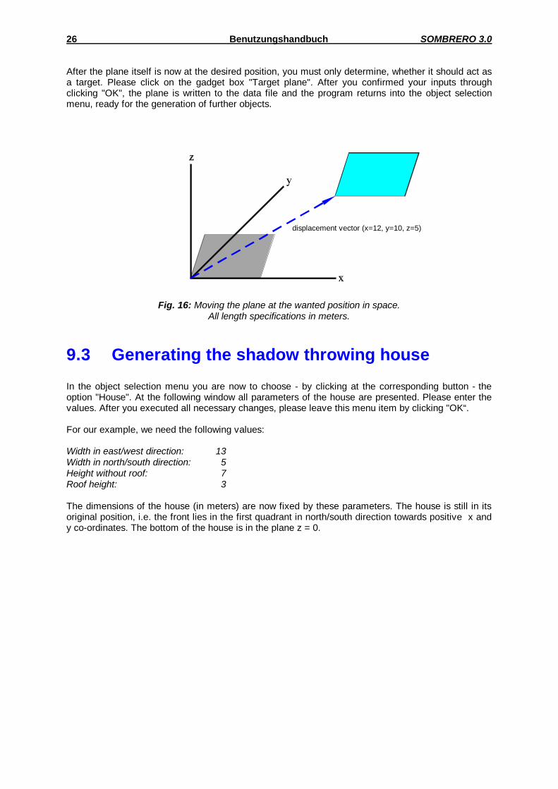
After the plane itself is now at the desired position, you must only determine, whether it should act as a target. Please click on the gadget box "Target plane". After you confirmed your inputs through clicking "OK", the plane is written to the data file and the program returns into the object selection menu, ready for the generation of further objects.

displacement vector (x=12, y=10, z=5)

Fig. 16: Moving the plane at the wanted position in space. All length specifications in meters.

9.3 Generating the shadow throwing house In the object selection menu you are now to choose - by clicking at the corresponding button - the option "House". At the following window all parameters of the house are presented. Please enter the values. After you executed all necessary changes, please leave this menu item by clicking "OK“. For our example, we need the following values: Width in east/west direction: 13 Width in north/south direction: 5 Height without roof: 7 Roof height: 3 The dimensions of the house (in meters) are now fixed by these parameters. The house is still in its original position, i.e. the front lies in the first quadrant in north/south direction towards positive x and y co-ordinates. The bottom of the house is in the plane z = 0.


Fig. 17: Location of the house in its original

position. The house is located in the plane z = 0 in the first quadrant.

Fig. 18: : View onto the x-y plane. The ridge is marked as a thick line in the y-

direction (north-south direction).

All length specifications in meters. In our example the broader side of the house should lie in east-west direction. This means that the house must be rotated around the z-axis by 90 degrees. Please enter at "Rotation of the house clockwise ..." the value 90°.

Fig. 19: Position of the house after the rotation

by 90 degrees around the z-axis.

Fig. 20: View at the x-y plane after the rotation. The ridge is now positioned in

west-east direction (x-direction).

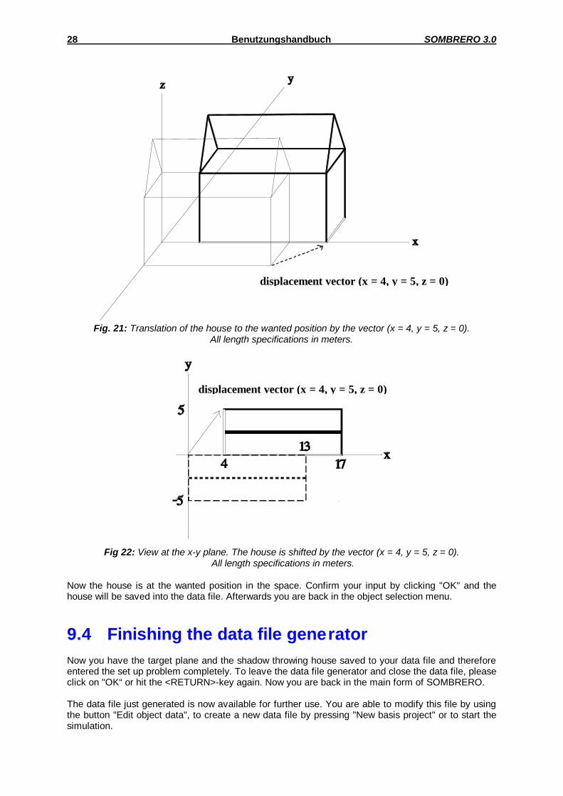
All length specifications in meters. Finally, the house has to be moved at the wanted position in the x-y-z system. For this a shift by the vector (x = 4, y = 5, z = 0) is necessary. Please enter these three values at "Translation by the vector...“.


displacement vector (x = 4, y = 5, z = 0)

Fig. 21: Translation of the house to the wanted position by the vector (x = 4, y = 5, z = 0).

All length specifications in meters.

displacement vector (x = 4, y = 5, z = 0)

Fig 22: View at the x-y plane. The house is shifted by the vector (x = 4, y = 5, z = 0).

All length specifications in meters. Now the house is at the wanted position in the space. Confirm your input by clicking "OK" and the house will be saved into the data file. Afterwards you are back in the object selection menu.

9.4 Finishing the data file generator Now you have the target plane and the shadow throwing house saved to your data file and therefore entered the set up problem completely. To leave the data file generator and close the data file, please click on "OK“ or hit the <RETURN>-key again. Now you are back in the main form of SOMBRERO. The data file just generated is now available for further use. You are able to modify this file by using the button "Edit object data", to create a new data file by pressing "New basis project" or to start the simulation.


9.5 VRML view of the project data Click the button "VRML view" to see the given data 3-dimensional with the help of a VRML player. If the program does not find a VRML player on your system, please follow the instruction given in Chapter 2.5.

10 Calculation of diffuse radiation with SOMBRERO

10.1 Motivation The majority of the thermal simulation programs calculate the diffuse radiation incident on inclined planes with regard to plane-related parameters like elevation ε with the method of Duffie & Beckman (1980)2, (Equation 1). The influence of objects like buildings and trees in the environment of the examined plane is neglected. For example, if a house is positioned next to a window which has to be examined, the incident diffuse radiation is extremely reduced. Moreover, the diffuse radiation at inclined planes depends on the reflection coefficient ρ of the earth’s surface. Usually this parameter is not constant, but is varying in the course of the year, e.g. by snowfall. SOMBRERO considers as well the influence of obstacles as the time related variation of the ground reflection coefficient ρ.

The calculation of the factors νS and νG is explained in the following. They can be imported by simulation programs as monthly varying parameters. The radiation intensities Hdhor and Hbhor are calculated as usual by the radiation processor of the thermal or photovoltaic simulation programs basing on measured weather data and are multiplied by the geometric-related factors found by SOMBRERO. A connection like this was conducted with TRNSYS 14.1 and is described in Niewienda & Heidt (1996)3.

2 Duffie J.A., Beckman W.A. (1980) Solar engineering of thermal processes. John Wiley & Sons,

Inc., New York, p. 86. 3 Niewienda A., Heidt F.D.: SOMBRERO, a PC-tool to calculate shadows on arbitrarily oriented

surfaces. Solar Energy, Vol. 58, No. 4 - 6, pp. 253 - 263, 1996

( )

( ) GdhorbhorSdhor

dhorbhordhord

HHH2sin1

HH2sin1

H)(H

ν⋅++ν⋅=

ε−⋅ρ⋅++

ε+⋅=ε

(Eq. 1)

with

Hdhor: Diffuse radiation onto the horizontal plane Hbhor: Direct radiation onto the horizontal plane ρ: Ground reflection coefficient (varying monthly) ε: Elevation of the surface νS View-Factor for the sky νG Ground-factor


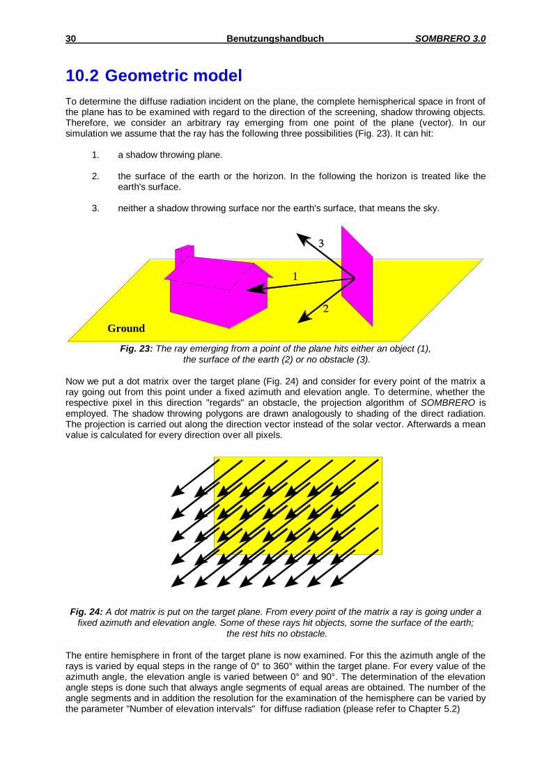
10.2 Geometric model To determine the diffuse radiation incident on the plane, the complete hemispherical space in front of the plane has to be examined with regard to the direction of the screening, shadow throwing objects. Therefore, we consider an arbitrary ray emerging from one point of the plane (vector). In our simulation we assume that the ray has the following three possibilities (Fig. 23). It can hit:

1. a shadow throwing plane. 2. the surface of the earth or the horizon. In the following the horizon is treated like the

earth's surface. 3. neither a shadow throwing surface nor the earth's surface, that means the sky.

Ground

Fig. 23: The ray emerging from a point of the plane hits either an object (1), the surface of the earth (2) or no obstacle (3).

Now we put a dot matrix over the target plane (Fig. 24) and consider for every point of the matrix a ray going out from this point under a fixed azimuth and elevation angle. To determine, whether the respective pixel in this direction "regards" an obstacle, the projection algorithm of SOMBRERO is employed. The shadow throwing polygons are drawn analogously to shading of the direct radiation. The projection is carried out along the direction vector instead of the solar vector. Afterwards a mean value is calculated for every direction over all pixels.

Fig. 24: A dot matrix is put on the target plane. From every point of the matrix a ray is going under a fixed azimuth and elevation angle. Some of these rays hit objects, some the surface of the earth;

the rest hits no obstacle.

The entire hemisphere in front of the target plane is now examined. For this the azimuth angle of the rays is varied by equal steps in the range of 0° to 360° within the target plane. For every value of the azimuth angle, the elevation angle is varied between 0° and 90°. The determination of the elevation angle steps is done such that always angle segments of equal areas are obtained. The number of the angle segments and in addition the resolution for the examination of the hemisphere can be varied by the parameter "Number of elevation intervals" for diffuse radiation (please refer to Chapter 5.2)


10.3 Weighting factors For the determination of the factors νS and νG it is first determined, whether the direction vector is set to the sky or set to the ground. The ground reflects direct radiation and diffuse sky radiation, whereas the sky emits (as model assumption) only isotropic diffuse radiation. Further is assumed, that the surfaces of shadow throwing objects only reflect the diffuse part of the total radiation. These planes are therefore added to the sky, independent of the fact whether the direction vector is indicated upwards or downwards. The reason for this assumption is, that on the temporal and spatial average a shadow throwing surface receives mainly diffuse radiation. Example: The shading of a southern facade should be computed. So possible obstacles will be

mainly located at the northern side. This side only "sees" direct sunlight in the midsummer immediately after sunrise and before sunset.

The reflection coefficient of the diffuse radiation from targets can be adjusted by the user via the parameter "Reflection coefficient of obstacles". Like we mentioned already above, every ray is equipped with a weighting factor, depending on which of the three possibilities applies to it. We will briefly explain these factors here: 1. The ray strikes a shadow throwing plane.

The incident diffuse radiation from this direction is reduced through the plane in the path. The weighting factor in this case is set the value of the parameter "Reflection coefficient of obstacles". If the shadow throwing object is a tree, a monthly changing foliage coefficient is considered. Example: The value of the foliage coefficient (from the schedule/foliage) amounts 60%. For

the determination of the weighting factor, 60% of a ray set to the sky are weighted with the factor 0,2 (object). The remaining 40% of the ray are weighted with the factor 1 (ray ends in the infinity, see 3). As a result we have: Weighting factor = 0,6 × 0,2 + 0,4 × 1 = 0,52.

2. The ray strikes the earth's surface.

The weighting factor remounts in this case from ground reverberation, which may vary in the year’s temporal course (i.e. by snow in the winter). To consider these circumstances, a separate weighting factor for every month may be determined.

3. The ray strikes no obstacle.

In this case the weighting factor is normally set to the reduction coefficient for sky radiation, because the incident diffuse radiation is not influenced by other objects or a special property of the earth’s surface.

Further, every ray is - according to Lambert’s law - multiplied with the cosine of its distance angle from the targets normal vector.


10.4 Determination with the project algorithm For the calculation of the weighting factor the projection algorithm used also for shadow calculation is employed. Here is proceeded as follows: At first the projection vector is set to a fixed azimuth and elevation angle. Then all available objects along this vector are projected with the projection algorithm onto the target face. Now every point of the target plane is checked by means of its color, which of the three possibilities applies for the ray that goes out from this point of the plane and runs along the projection vector: • The point has the color of the target face (light blue) :

Now it must be examined, whether the defined elevation angle is smaller than or equal to the horizon angle. In this case, the ray hits either the earth's surface or the horizon (possibility 2) and receives the monthly weighting factor determined by the user. If the elevation angle is larger than the horizon angle, the ray encounters neither onto the earth nor onto an object (possibility 3) and receives the weighting factor "Reduction coefficient for sky radiation".

• The point has the color of a tree (light green):

In this case the ray strikes the foliaged face of a tree, and the weighting factor is computed considering the foliage coefficient. (possibility 1, calculation example).

• The point has a different color:

In this case the ray hits a shadow throwing plane (object) and receives the weighting factor of the ground reflection coefficient (possibility 1).

Like already described, all weighted rays are averaged to a plane weighting factor dependent on their inclination (to the sky or the ground). The mean value for the different angles is equal to the final weighting factors νS and νG for diffuse radiation.

11 Limited liability The specification contained in this manual is without guarantee and can be changed without further notification. The program developers don’t have hereby any obligation. From the application of the program no liability claims are derivable. It is incumbent on the user to check the plausibility and correctness of any results obtained with the program by a professional check.


12 Comments / Suggestions If you have questions or suggestions to improve the program, please contact us. Your comments will be a an essential help for the further development of SOMBRERO. Please send your comments to: Prof. Dr.-Ing. F.D. Heidt T: +49-271-740-3817 Fachgebiet Bauphysik & Solarenergie F: +49-271-740-3820 Universität-Gesamthochschule Siegen E: [email protected] D - 57068 Siegen W: http://nesa1.uni-siegen.de/ Germany

Documents

SOMBRERO USer Manual - Censolar - CENSOLAR (Centro de Estudios de