Embed Size (px)
Citation preview

6Solving Nonlinear Algebraic Equations
As a reader of this book you are probably well into mathematics and often “ac-cused” of being particularly good at “solving equations” (a typical comment atfamily dinners!). However, is it really true that you, with pen and paper, can solvemany types of equations? Restricting our attention to algebraic equations in oneunknown x, you can certainly do linear equations: ax C b D 0, and quadratic ones:ax2 C bx C c D 0. You may also know that there are formulas for the roots of cu-bic and quartic equations too. Maybe you can do the special trigonometric equationsin x C cosx D 1 as well, but there it (probably) stops. Equations that are not re-ducible to one of the mentioned cannot be solved by general analytical techniques,which means that most algebraic equations arising in applications cannot be treatedwith pen and paper!
If we exchange the traditional idea of finding exact solutions to equations withthe idea of rather finding approximate solutions, a whole new world of possibilitiesopens up. With such an approach, we can in principle solve any algebraic equation.
Let us start by introducing a common generic form for any algebraic equation:
f .x/ D 0 :
Here, f .x/ is some prescribed formula involving x. For example, the equation
e�x sin x D cosx
185© The Author(s) 2016S. Linge, H.P. Langtangen, Programming for Computations – Python,Texts in Computational Science and Engineering 15, DOI 10.1007/978-3-319-32428-9_6
186 6 Solving Nonlinear Algebraic Equations
hasf .x/ D e�x sin x � cosx :
Just move all terms to the left-hand side and then the formula to the left of theequality sign is f .x/.
So, when do we really need to solve algebraic equations beyond the simplesttypes we can treat with pen and paper? There are two major application areas. Oneis when using implicit numerical methods for ordinary differential equations. Thesegive rise to one or a system of algebraic equations. The other major application typeis optimization, i.e., finding the maxima or minima of a function. These maxima andminima are normally found by solving the algebraic equation F 0.x/ D 0 if F.x/ isthe function to be optimized. Differential equations are very much used throughoutscience and engineering, and actually most engineering problems are optimizationproblems in the end, because one wants a design that maximizes performance andminimizes cost.
We first consider one algebraic equation in one variable, with our usual emphasison how to program the algorithms. Systems of nonlinear algebraic equations withmany variables arise from implicit methods for ordinary and partial differentialequations as well as in multivariate optimization. Our attention will be restricted toNewton’s method for such systems of nonlinear algebraic equations.
TerminologyWhen solving algebraic equations f .x/ D 0, we often say that the solution x
is a root of the equation. The solution process itself is thus often called rootfinding.
6.1 Brute Force Methods
The representation of a mathematical function f .x/ on a computer takes two forms.One is a Python function returning the function value given the argument, while theother is a collection of points .x; f .x// along the function curve. The latter is therepresentation we use for plotting, together with an assumption of linear variationbetween the points. This representation is also very suited for equation solvingand optimization: we simply go through all points and see if the function crossesthe x axis, or for optimization, test for a local maximum or minimum point. Be-cause there is a lot of work to examine a huge number of points, and also becausethe idea is extremely simple, such approaches are often referred to as brute forcemethods. However, we are not embarrassed of explaining the methods in detail andimplementing them.

6.1 Brute Force Methods 187
6.1.1 Brute Force Root Finding
Assume that we have a set of points along the curve of a function f .x/:
We want to solve f .x/ D 0, i.e., find the points x where f crosses the x axis.A brute force algorithm is to run through all points on the curve and check if onepoint is below the x axis and if the next point is above the x axis, or the other wayaround. If this is found to be the case, we know that f must be zero in betweenthese two x points.
Numerical algorithm More precisely, we have a set of n C 1 points .xi ; yi /, yi Df .xi /, i D 0; : : : ; n, where x0 < : : : < xn. We check if yi < 0 and yiC1 > 0 (orthe other way around). A compact expression for this check is to perform the testyi yiC1 < 0. If so, the root of f .x/ D 0 is in Œxi ; xiC1�. Assuming a linear variationof f between xi and xiC1, we have the approximation
f .x/ � f .xiC1/ � f .xi /
xiC1 � xi
.x � xi / C f .xi / D yiC1 � yi
xiC1 � xi
.x � xi / C yi ;
which, when set equal to zero, gives the root
x D xi � xiC1 � xi
yiC1 � yi
yi :
Implementation Given some Python implementation f(x) of our mathematicalfunction, a straightforward implementation of the above numerical algorithm lookslike
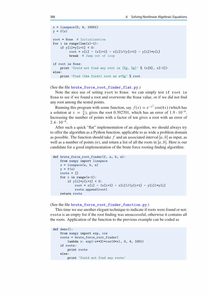
188 6 Solving Nonlinear Algebraic Equations
x = linspace(0, 4, 10001)
y = f(x)
root = None # Initialization
for i in range(len(x)-1):
if y[i]*y[i+1] < 0:
root = x[i] - (x[i+1] - x[i])/(y[i+1] - y[i])*y[i]
break # Jump out of loop
if root is None:
print ’Could not find any root in [%g, %g]’ % (x[0], x[-1])
else:
print ’Find (the first) root as x=%g’ % root
(See the file brute_force_root_finder_flat.py.)Note the nice use of setting root to None: we can simply test if root is
None to see if we found a root and overwrote the None value, or if we did not findany root among the tested points.
Running this program with some function, say f .x/ D e�x2cos.4x/ (which has
a solution at x D �8), gives the root 0.392701, which has an error of 1:9 � 10�6.
Increasing the number of points with a factor of ten gives a root with an error of2:4 � 10�8.
After such a quick “flat” implementation of an algorithm, we should always tryto offer the algorithm as a Python function, applicable to as wide a problem domainas possible. The function should take f and an associated interval Œa; b� as input, aswell as a number of points (n), and return a list of all the roots in Œa; b�. Here is ourcandidate for a good implementation of the brute force rooting finding algorithm:
def brute_force_root_finder(f, a, b, n):
from numpy import linspace
x = linspace(a, b, n)
y = f(x)
roots = []
for i in range(n-1):
if y[i]*y[i+1] < 0:
root = x[i] - (x[i+1] - x[i])/(y[i+1] - y[i])*y[i]
roots.append(root)
return roots
(See the file brute_force_root_finder_function.py.)This time we use another elegant technique to indicate if roots were found or not:
roots is an empty list if the root finding was unsuccessful, otherwise it contains allthe roots. Application of the function to the previous example can be coded as
def demo():
from numpy import exp, cos
roots = brute_force_root_finder(
lambda x: exp(-x**2)*cos(4*x), 0, 4, 1001)
if roots:
print roots
else:
print ’Could not find any roots’

6.1 Brute Force Methods 189
Note that if roots evaluates to True if roots is non-empty. This is a generaltest in Python: if X evaluates to True if X is non-empty or has a nonzero value.
6.1.2 Brute Force Optimization
Numerical algorithm We realize that xi corresponds to a maximum point ifyi�1 < yi > yiC1. Similarly, xi corresponds to a minimum if yi�1 > yi < yiC1.We can do this test for all “inner” points i D 1; : : : ; n � 1 to find all local minimaand maxima. In addition, we need to add an end point, i D 0 or i D n, if thecorresponding yi is a global maximum or minimum.
Implementation The algorithm above can be translated to the following Pythonfunction (file brute_force_optimizer.py):
def brute_force_optimizer(f, a, b, n):
from numpy import linspace
x = linspace(a, b, n)
y = f(x)
# Let maxima and minima hold the indices corresponding
# to (local) maxima and minima points
minima = []
maxima = []
for i in range(n-1):
if y[i-1] < y[i] > y[i+1]:
maxima.append(i)
if y[i-1] > y[i] < y[i+1]:
minima.append(i)
# What about the end points?
y_max_inner = max([y[i] for i in maxima])
y_min_inner = min([y[i] for i in minima])
if y[0] > y_max_inner:
maxima.append(0)
if y[len(x)-1] > y_max_inner:
maxima.append(len(x)-1)
if y[0] < y_min_inner:
minima.append(0)
if y[len(x)-1] < y_min_inner:
minima.append(len(x)-1)
# Return x and y values
return [(x[i], y[i]) for i in minima], \
[(x[i], y[i]) for i in maxima]
The max and min functions are standard Python functions for finding the maxi-mum and minimum element of a list or an object that one can iterate over with a forloop.
190 6 Solving Nonlinear Algebraic Equations
An application to f .x/ D e�x2cos.4x/ looks like
def demo():
from numpy import exp, cos
minima, maxima = brute_force_optimizer(
lambda x: exp(-x**2)*cos(4*x), 0, 4, 1001)
print ’Minima:’, minima
print ’Maxima:’, maxima
6.1.3 Model Problem for Algebraic Equations
We shall consider the very simple problem of finding the square root of 9, whichis the positive solution of x2 D 9. The nice feature of solving an equation whosesolution is known beforehand is that we can easily investigate how the numericalmethod and the implementation perform in the search for the solution. The f .x/
function corresponding to the equation x2 D 9 is
f .x/ D x2 � 9 :
Our interval of interest for solutions will be Œ0; 1000� (the upper limit here is chosensomewhat arbitrarily).
In the following, we will present several efficient and accurate methods for solv-ing nonlinear algebraic equations, both single equation and systems of equations.The methods all have in common that they search for approximate solutions. Themethods differ, however, in the way they perform the search for solutions. The ideafor the search influences the efficiency of the search and the reliability of actuallyfinding a solution. For example, Newton’s method is very fast, but not reliable,while the bisection method is the slowest, but absolutely reliable. No method isbest at all problems, so we need different methods for different problems.
What is the difference between linear and nonlinear equations?You know how to solve linear equations ax C b D 0: x D �b=a. All othertypes of equations f .x/ D 0, i.e., when f .x/ is not a linear function of x, arecalled nonlinear. A typical way of recognizing a nonlinear equation is to observethat x is “not alone” as in ax, but involved in a product with itself, such as inx3 C 2x2 � 9 D 0. We say that x3 and 2x2 are nonlinear terms. An equation likesin x C ex cosx D 0 is also nonlinear although x is not explicitly multiplied byitself, but the Taylor series of sin x, ex , and cosx all involve polynomials of x
where x is multiplied by itself.
6.2 Newton’s Method
Newton’s method, also known as Newton-Raphson’s method, is a very famous andwidely used method for solving nonlinear algebraic equations. Compared to theother methods we will consider, it is generally the fastest one (usually by far). Itdoes not guarantee that an existing solution will be found, however.
6.2 Newton’s Method 191
A fundamental idea of numerical methods for nonlinear equations is to constructa series of linear equations (since we know how to solve linear equations) and hopethat the solutions of these linear equations bring us closer and closer to the solutionof the nonlinear equation. The idea will be clearer when we present Newton’smethod and the secant method.
6.2.1 Deriving and Implementing Newton’sMethod
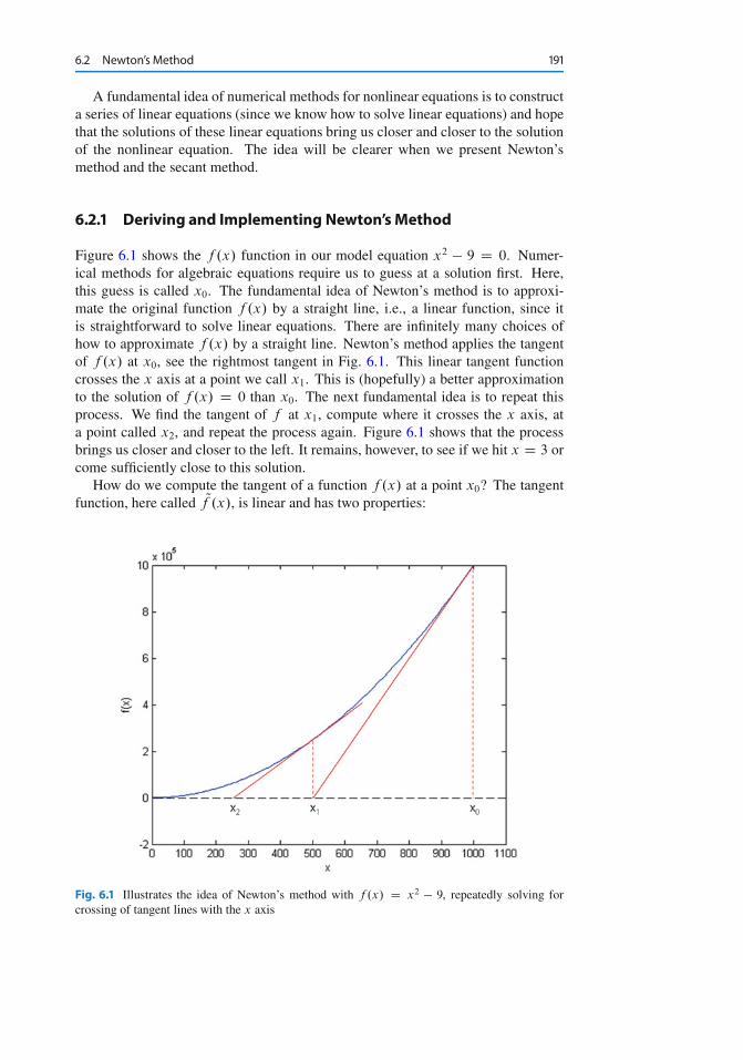
Figure 6.1 shows the f .x/ function in our model equation x2 � 9 D 0. Numer-ical methods for algebraic equations require us to guess at a solution first. Here,this guess is called x0. The fundamental idea of Newton’s method is to approxi-mate the original function f .x/ by a straight line, i.e., a linear function, since itis straightforward to solve linear equations. There are infinitely many choices ofhow to approximate f .x/ by a straight line. Newton’s method applies the tangentof f .x/ at x0, see the rightmost tangent in Fig. 6.1. This linear tangent functioncrosses the x axis at a point we call x1. This is (hopefully) a better approximationto the solution of f .x/ D 0 than x0. The next fundamental idea is to repeat thisprocess. We find the tangent of f at x1, compute where it crosses the x axis, ata point called x2, and repeat the process again. Figure 6.1 shows that the processbrings us closer and closer to the left. It remains, however, to see if we hit x D 3 orcome sufficiently close to this solution.
How do we compute the tangent of a function f .x/ at a point x0? The tangentfunction, here called Qf .x/, is linear and has two properties:
Fig. 6.1 Illustrates the idea of Newton’s method with f .x/ D x2 � 9, repeatedly solving forcrossing of tangent lines with the x axis
192 6 Solving Nonlinear Algebraic Equations
1. the slope equals to f 0.x0/
2. the tangent touches the f .x/ curve at x0
So, if we write the tangent function as Qf .x/ D ax C b, we must require Qf 0.x0/ Df 0.x0/ and Qf .x0/ D f .x0/, resulting in
Qf .x/ D f .x0/ C f 0.x0/.x � x0/ :
The key step in Newton’s method is to find where the tangent crosses the x axis,which means solving Qf .x/ D 0:
Qf .x/ D 0 ) x D x0 � f .x0/
f 0.x0/:
This is our new candidate point, which we call x1:
x1 D x0 � f .x0/
f 0.x0/:
With x0 D 1000, we get x1 � 500, which is in accordance with the graph inFig. 6.1. Repeating the process, we get
x2 D x1 � f .x1/
f 0.x1/� 250 :
The general scheme of Newton’s method may be written as
xnC1 D xn � f .xn/
f 0.xn/; n D 0; 1; 2; : : : (6.1)
The computation in (6.1) is repeated until f .xn/ is close enough to zero. Moreprecisely, we test if jf .xn/j < �, with � being a small number.
We moved from 1000 to 250 in two iterations, so it is exciting to see howfast we can approach the solution x D 3. A computer program can automatethe calculations. Our first try at implementing Newton’s method is in a functionnaive_Newton:
def naive_Newton(f, dfdx, x, eps):
while abs(f(x)) > eps:
x = x - float(f(x))/dfdx(x)
return x
The argument x is the starting value, called x0 in our previous mathematical de-scription. We use float(f(x)) to ensure that an integer division does not happenby accident if f(x) and dfdx(x) both are integers for some x.
To solve the problem x2 D 9 we also need to implement
def f(x):
return x**2 - 9
def dfdx(x):
return 2*x
print naive_Newton(f, dfdx, 1000, 0.001)
6.2 Newton’s Method 193
Why not use an array for the x approximations?Newton’s method is normally formulated with an iteration index n,
xnC1 D xn � f .xn/
f 0.xn/:
Seeing such an index, many would implement this as
x[n+1] = x[n] - f(x[n])/dfdx(x[n])
Such an array is fine, but requires storage of all the approximations. In largeindustrial applications, where Newton’s method solves millions of equations atonce, one cannot afford to store all the intermediate approximations in memory,so then it is important to understand that the algorithm in Newton’s method hasno more need for xn when xnC1 is computed. Therefore, we can work with onevariable x and overwrite the previous value:
x = x - f(x)/dfdx(x)
Running naive_Newton(f, dfdx, 1000, eps=0.001) results in the ap-proximate solution 3.000027639. A smaller value of eps will produce a moreaccurate solution. Unfortunately, the plain naive_Newton function does not re-turn how many iterations it used, nor does it print out all the approximationsx0; x1; x2; : : :, which would indeed be a nice feature. If we insert such a printout,a rerun results in
500.0045
250.011249919
125.02362415
62.5478052723
31.3458476066
15.816483488
8.1927550496
4.64564330569
3.2914711388
3.01290538807
3.00002763928
We clearly see that the iterations approach the solution quickly. This speed ofthe search for the solution is the primary strength of Newton’s method compared toother methods.
6.2.2 Making aMore Efficient and Robust Implementation
The naive_Newton function works fine for the example we are considering here.However, for more general use, there are some pitfalls that should be fixed in animproved version of the code. An example may illustrate what the problem is: letus solve tanh.x/ D 0, which has solution x D 0. With jx0j � 1:08 everythingworks fine. For example, x0 leads to six iterations if � D 0:001:

194 6 Solving Nonlinear Algebraic Equations
-1.05895313436
0.989404207298
-0.784566773086
0.36399816111
-0.0330146961372
2.3995252668e-05
Adjusting x0 slightly to 1.09 gives division by zero! The approximations com-puted by Newton’s method become
-1.09331618202
1.10490354324
-1.14615550788
1.30303261823
-2.06492300238
13.4731428006
-1.26055913647e+11
The division by zero is caused by x7 D �1:26055913647�1011, because tanh.x7/
is 1.0 to machine precision, and then f 0.x/ D 1 � tanh.x/2 becomes zero in thedenominator in Newton’s method.
The underlying problem, leading to the division by zero in the above example,is that Newton’s method diverges: the approximations move further and furtheraway from x D 0. If it had not been for the division by zero, the condition inthe while loop would always be true and the loop would run forever. Divergenceof Newton’s method occasionally happens, and the remedy is to abort the methodwhen a maximum number of iterations is reached.
Another disadvantage of the naive_Newton function is that it calls the f .x/
function twice as many times as necessary. This extra work is of no concern whenf .x/ is fast to evaluate, but in large-scale industrial software, one call to f .x/ mighttake hours or days, and then removing unnecessary calls is important. The solutionin our function is to store the call f(x) in a variable (f_value) and reuse the valueinstead of making a new call f(x).
To summarize, we want to write an improved function for implementing New-ton’s method where we
� avoid division by zero� allow a maximum number of iterations� avoid the extra evaluation of f .x/
A more robust and efficient version of the function, inserted in a complete programNewtons_method.py for solving x2 � 9 D 0, is listed below.
def Newton(f, dfdx, x, eps):
f_value = f(x)
iteration_counter = 0
while abs(f_value) > eps and iteration_counter < 100:
try:
x = x - float(f_value)/dfdx(x)

6.2 Newton’s Method 195
except ZeroDivisionError:
print "Error! - derivative zero for x = ", x
sys.exit(1) # Abort with error
f_value = f(x)
iteration_counter += 1
# Here, either a solution is found, or too many iterations
if abs(f_value) > eps:
iteration_counter = -1
return x, iteration_counter
def f(x):
return x**2 - 9
def dfdx(x):
return 2*x
solution, no_iterations = Newton(f, dfdx, x=1000, eps=1.0e-6)
if no_iterations > 0: # Solution found
print "Number of function calls: %d" % (1 + 2*no_iterations)
print "A solution is: %f" % (solution)
else:
print "Solution not found!"
Handling of the potential division by zero is done by a try-except construction.Python tries to run the code in the try block. If anything goes wrong here, or moreprecisely, if Python raises an exception caused by a problem (such as division byzero, array index out of bounds, use of undefined variable, etc.), the execution jumpsimmediately to the except block. Here, the programmer can take appropriate ac-tions. In the present case, we simply stop the program. (Professional programmerswould avoid calling sys.exit inside a function. Instead, they would raise a newexception with an informative error message, and let the calling code have anothertry-except construction to stop the program.)
The division by zero will always be detected and the program will be stopped.The main purpose of our way of treating the division by zero is to give the usera more informative error message and stop the program in a gentler way.
Calling sys.exit with an argument different from zero (here 1) signifies thatthe program stopped because of an error. It is a good habit to supply the value 1,because tools in the operating system can then be used by other programs to detectthat our program failed.
To prevent an infinite loop because of divergent iterations, we have introducedthe integer variable iteration_counter to count the number of iterations in New-ton’s method. With iteration_counterwe can easily extend the condition in thewhile such that no more iterations take place when the number of iterations reaches100. We could easily let this limit be an argument to the function rather than a fixedconstant.
The Newton function returns the approximate solution and the number of itera-tions. The latter equals �1 if the convergence criterion jf .x/j < � was not reachedwithin the maximum number of iterations. In the calling code, we print out the
196 6 Solving Nonlinear Algebraic Equations
solution and the number of function calls. The main cost of a method for solvingf .x/ D 0 equations is usually the evaluation of f .x/ and f 0.x/, so the total num-ber of calls to these functions is an interesting measure of the computational work.Note that in function Newton there is an initial call to f .x/ and then one call to f
and one to f 0 in each iteration.Running Newtons_method.py, we get the following printout on the screen:
Number of function calls: 25
A solution is: 3.000000
As we did with the integration methods in Chapter 3, we will collect our solversfor nonlinear algebraic equations in a separate file named nonlinear_solvers.pyfor easy import and use. The first function placed in this file is then Newton.
The Newton scheme will work better if the starting value is close to the solution.A good starting value may often make the difference as to whether the code actuallyfinds a solution or not. Because of its speed, Newton’s method is often the methodof first choice for solving nonlinear algebraic equations, even if the scheme is notguaranteed to work. In cases where the initial guess may be far from the solution,a good strategy is to run a few iterations with the bisection method (see Chapter 6.4)to narrow down the region where f is close to zero and then switch to Newton’smethod for fast convergence to the solution.
Newton’s method requires the analytical expression for the derivative f 0.x/.Derivation of f 0.x/ is not always a reliable process by hand if f .x/ is a com-plicated function. However, Python has the symbolic package SymPy, which wemay use to create the required dfdx function. In our sample problem, the recipegoes as follows:
from sympy import *
x = symbols(’x’) # define x as a mathematical symbol
f_expr = x**2 - 9 # symbolic expression for f(x)
dfdx_expr = diff(f_expr, x) # compute f’(x) symbolically
# Turn f_expr and dfdx_expr into plain Python functions
f = lambdify([x], # argument to f
f_expr) # symbolic expression to be evaluated
dfdx = lambdify([x], dfdx_expr)
print dfdx(5) # will print 10
The nice feature of this code snippet is that dfdx_expr is the exact analyticalexpression for the derivative, 2*x, if you print it out. This is a symbolic expressionso we cannot do numerical computing with it, but the lambdify constructions turnsymbolic expressions into callable Python functions.
The next method is the secant method, which is usually slower than Newton’smethod, but it does not require an expression for f 0.x/, and it has only one functioncall per iteration.

6.3 The Secant Method 197
6.3 The Secant Method
When finding the derivative f 0.x/ in Newton’s method is problematic, or whenfunction evaluations take too long; we may adjust the method slightly. Instead ofusing tangent lines to the graph we may use secants1. The approach is referred to asthe secant method, and the idea is illustrated graphically in Fig. 6.2 for our exampleproblem x2 � 9 D 0.
The idea of the secant method is to think as in Newton’s method, but insteadof using f 0.xn/, we approximate this derivative by a finite difference or the se-cant, i.e., the slope of the straight line that goes through the points .xn; f .xn// and.xn�1; f .xn�1// on the graph, given by the two most recent approximations xn andxn�1. This slope reads
f .xn/ � f .xn�1/
xn � xn�1
: (6.2)
Inserting this expression for f 0.xn/ in Newton’s method simply gives us the secantmethod:
xnC1 D xn � f .xn/f .xn/�f .xn�1/
xn�xn�1
;
orxnC1 D xn � f .xn/
xn � xn�1
f .xn/ � f .xn�1/: (6.3)
Fig. 6.2 Illustrates the use of secants in the secant method when solving x2�9 D 0; x 2 Œ0; 1000�.From two chosen starting values, x0 D 1000 and x1 D 700 the crossing x2 of the correspondingsecant with the x axis is computed, followed by a similar computation of x3 from x1 and x2
1 https://en.wikipedia.org/wiki/Secant_line
198 6 Solving Nonlinear Algebraic Equations
Comparing (6.3) to the graph in Fig. 6.2, we see how two chosen starting points(x0 D 1000, x1 D 700, and corresponding function values) are used to computex2. Once we have x2, we similarly use x1 and x2 to compute x3. As with Newton’smethod, the procedure is repeated until f .xn/ is below some chosen limit value,or some limit on the number of iterations has been reached. We use an iterationcounter here too, based on the same thinking as in the implementation of Newton’smethod.
We can store the approximations xn in an array, but as in Newton’s method,we notice that the computation of xnC1 only needs knowledge of xn and xn�1, not“older” approximations. Therefore, we can make use of only three variables: x forxnC1, x1 for xn, and x0 for xn�1. Note that x0 and x1 must be given (guessed) forthe algorithm to start.
A program secant_method.py that solves our example problemmay be writtenas:
def secant(f, x0, x1, eps):
f_x0 = f(x0)
f_x1 = f(x1)
iteration_counter = 0
while abs(f_x1) > eps and iteration_counter < 100:
try:
denominator = float(f_x1 - f_x0)/(x1 - x0)
x = x1 - float(f_x1)/denominator
except ZeroDivisionError:
print "Error! - denominator zero for x = ", x
sys.exit(1) # Abort with error
x0 = x1
x1 = x
f_x0 = f_x1
f_x1 = f(x1)
iteration_counter += 1
# Here, either a solution is found, or too many iterations
if abs(f_x1) > eps:
iteration_counter = -1
return x, iteration_counter
def f(x):
return x**2 - 9
x0 = 1000; x1 = x0 - 1
solution, no_iterations = secant(f, x0, x1, eps=1.0e-6)
if no_iterations > 0: # Solution found
print "Number of function calls: %d" % (2 + no_iterations)
print "A solution is: %f" % (solution)
else:
print "Solution not found!"
The number of function calls is now related to no_iterations, i.e., the numberof iterations, as 2 + no_iterations, since we need two function calls before en-tering the while loop, and then one function call per loop iteration. Note that, eventhough we need two points on the graph to compute each updated estimate, only
6.4 The Bisection Method 199
a single function call (f(x1)) is required in each iteration since f(x0) becomes the“old” f(x1) and may simply be copied as f_x0 = f_x1 (the exception is the veryfirst iteration where two function evaluations are needed).
Running secant_method.py, gives the following printout on the screen:
Number of function calls: 19
A solution is: 3.000000
Aswith the function Newton, we place secant in the file nonlinear_solvers.py for easy import and use later.
6.4 The BisectionMethod
Neither Newton’s method nor the secant method can guarantee that an existing so-lution will be found (see Exercises 6.1 and 6.2). The bisection method, however,does that. However, if there are several solutions present, it finds only one of them,just as Newton’s method and the secant method. The bisection method is slowerthan the other two methods, so reliability comes with a cost of speed.
To solve x2 � 9 D 0, x 2 Œ0; 1000�, with the bisection method, we reason asfollows. The first key idea is that if f .x/ D x2 �9 is continuous on the interval andthe function values for the interval endpoints (xL D 0, xR D 1000) have oppositesigns, f .x/ must cross the x axis at least once on the interval. That is, we knowthere is at least one solution.
The second key idea comes from dividing the interval in two equal parts, oneto the left and one to the right of the midpoint xM D 500. By evaluating the signof f .xM /, we will immediately know whether a solution must exist to the left orright of xM . This is so, since if f .xM / � 0, we know that f .x/ has to cross the x
axis between xL and xM at least once (using the same argument as for the originalinterval). Likewise, if instead f .xM / � 0, we know that f .x/ has to cross the x
axis between xM and xR at least once.In any case, we may proceed with half the interval only. The exception is if
f .xM / � 0, in which case a solution is found. Such interval halving can becontinued until a solution is found. A “solution” in this case, is when jf .xM /jis sufficiently close to zero, more precisely (as before): jf .xM /j < �, where � isa small number specified by the user.
The sketched strategy seems reasonable, so let us write a reusable function thatcan solve a general algebraic equation f .x/ D 0 (bisection_method.py):
def bisection(f, x_L, x_R, eps, return_x_list=False):
f_L = f(x_L)
if f_L*f(x_R) > 0:
print "Error! Function does not have opposite \
signs at interval endpoints!"
sys.exit(1)
x_M = float(x_L + x_R)/2.0
f_M = f(x_M)
iteration_counter = 1

200 6 Solving Nonlinear Algebraic Equations
if return_x_list:
x_list = []
while abs(f_M) > eps:
if f_L*f_M > 0: # i.e. same sign
x_L = x_M
f_L = f_M
else:
x_R = x_M
x_M = float(x_L + x_R)/2
f_M = f(x_M)
iteration_counter += 1
if return_x_list:
x_list.append(x_M)
if return_x_list:
return x_list, iteration_counter
else:
return x_M, iteration_counter
def f(x):
return x**2 - 9
a = 0; b = 1000
solution, no_iterations = bisection(f, a, b, eps=1.0e-6)
print "Number of function calls: %d" % (1 + 2*no_iterations)
print "A solution is: %f" % (solution)
Note that we first check if f changes sign in Œa; b�, because that is a requirementfor the algorithm to work. The algorithm also relies on a continuous f .x/ function,but this is very challenging for a computer code to check.
We get the following printout to the screen when bisection_method.py is run:
Number of function calls: 61
A solution is: 3.000000
We notice that the number of function calls is much higher than with the previousmethods.
Required work in the bisection methodIf the starting interval of the bisection method is bounded by a and b, and thesolution at step n is taken to be the middle value, the error is bounded as
jb � aj2n
; (6.4)
because the initial interval has been halved n times. Therefore, to meet a toler-ance �, we need n iterations such that the length of the current interval equals�: jb � aj
2nD � ) n D ln..b � a/=�/
ln 2:

6.5 Rate of Convergence 201
This is a great advantage of the bisection method: we know beforehand howmany iterations n it takes to meet a certain accuracy � in the solution.
As with the two previous methods, the function bisection is placed in the filenonlinear_solvers.py for easy import and use.
6.5 Rate of Convergence
With the methods above, we noticed that the number of iterations or function callscould differ quite substantially. The number of iterations needed to find a solutionis closely related to the rate of convergence, which dictates the speed of error re-duction as we approach the root. More precisely, we introduce the error in iterationn as en D jx � xnj, and define the convergence rate q as
enC1 D Ceqn; (6.5)
where C is a constant. The exponent q measures how fast the error is reduced fromone iteration to the next. The larger q is, the faster the error goes to zero, and thefewer iterations we need to meet the stopping criterion jf .x/j < �.
A single q in (6.5) is defined in the limit n ! 1. For finite n, and especiallysmaller n, q will vary with n. To estimate q, we can compute all the errors en andset up (6.5) for three consecutive experiments n � 1, n, and n C 1:
en D Ceqn�1;
enC1 D Ceqn :
Dividing these two equations by each other and solving with respect to q gives
q D ln.enC1=en/
ln.en=en�1/:
Since this q will vary somewhat with n, we call it qn. As n grows, we expect qn
to approach a limit (qn ! q). To compute all the qn values, we need all the xn
approximations. However, our previous implementations of Newton’s method, thesecant method, and the bisection method returned just the final approximation.
Therefore, we have extended the implementations in the module filenonlinear_solvers.py such that the user can choose whether the final valueor the whole history of solutions is to be returned. Each of the extended im-plementations now takes an extra parameter return_x_list. This parameter isa boolean, set to True if the function is supposed to return all the root approxima-tions, or False, if the function should only return the final approximation. As anexample, let us take a closer look at Newton:
def Newton(f, dfdx, x, eps, return_x_list=False):
f_value = f(x)
iteration_counter = 0
if return_x_list:
x_list = []

202 6 Solving Nonlinear Algebraic Equations
while abs(f_value) > eps and iteration_counter < 100:
try:
x = x - float(f_value)/dfdx(x)
except ZeroDivisionError:
print "Error! - derivative zero for x = ", x
sys.exit(1) # Abort with error
f_value = f(x)
iteration_counter += 1
if return_x_list:
x_list.append(x)
# Here, either a solution is found, or too many iterations
if abs(f_value) > eps:
iteration_counter = -1 # i.e., lack of convergence
if return_x_list:
return x_list, iteration_counter
else:
return x, iteration_counter
The function is found in the file nonlinear_solvers.py.We can now make a call
x, iter = Newton(f, dfdx, x=1000, eps=1e-6, return_x_list=True)
and get a list x returned. With knowledge of the exact solution x of f .x/ D 0
we can compute all the errors en and all the associated qn values with the compactfunction
def rate(x, x_exact):
e = [abs(x_ - x_exact) for x_ in x]
q = [log(e[n+1]/e[n])/log(e[n]/e[n-1])
for n in range(1, len(e)-1, 1)]
return q
The error model (6.5) works well for Newton’s method and the secant method.For the bisection method, however, it works well in the beginning, but not when thesolution is approached.
We can compute the rates qn and print them nicely,
def print_rates(method, x, x_exact):
q = [’%.2f’ % q_ for q_ in rate(x, x_exact)]
print method + ’:’
for q_ in q:
print q_,
The result for print_rates(’Newton’, x, 3) is
Newton:
1.01 1.02 1.03 1.07 1.14 1.27 1.51 1.80 1.97 2.00
6.6 Solving Multiple Nonlinear Algebraic Equations 203
indicating that q D 2 is the rate for Newton’s method. A similar computationusing the secant method, gives the rates
secant:
1.26 0.93 1.05 1.01 1.04 1.05 1.08 1.13 1.20 1.30 1.43
1.54 1.60 1.62 1.62
Here it seems that q � 1:6 is the limit.
Remark If we in the bisection method think of the length of the current intervalcontaining the solution as the error en, then (6.5) works perfectly since enC1 D12en, i.e., q D 1 and C D 1
2, but if en is the true error jx � xnj, it is easily seen
from a sketch that this error can oscillate between the current interval length anda potentially very small value as we approach the exact solution. The correspondingrates qn fluctuate widely and are of no interest.
6.6 Solving Multiple Nonlinear Algebraic Equations
So far in this chapter, we have considered a single nonlinear algebraic equation.However, systems of such equations arise in a number of applications, foremostnonlinear ordinary and partial differential equations. Of the previous algorithms,only Newton’s method is suitable for extension to systems of nonlinear equations.
6.6.1 Abstract Notation
Suppose we have n nonlinear equations, written in the following abstract form:
F0.x0; x1; : : : ; xn/ D 0; (6.6)
F1.x0; x1; : : : ; xn/ D 0; (6.7)
::: D ::: (6.8)
Fn.x0; x1; : : : ; xn/ D 0 : (6.9)
(6.10)
It will be convenient to introduce a vector notation
F D .F0; : : : ; F1/; x D .x0; : : : ; xn/ :
The system can now be written as F .x/ D 0.As a specific example on the notation above, the system
x2 D y � x cos.�x/ (6.11)
yx C e�y D x�1 (6.12)
204 6 Solving Nonlinear Algebraic Equations
can be written in our abstract form by introducing x0 D x and x1 D y. Then
F0.x0; x1/ D x2 � y C x cos.�x/ D 0;
F1.x0; x1/ D yx C e�y � x�1 D 0 :
6.6.2 Taylor Expansions for Multi-Variable Functions
We follow the ideas of Newton’s method for one equation in one variable: approxi-mate the nonlinear f by a linear function and find the root of that function. Whenn variables are involved, we need to approximate a vector function F .x/ by somelinear function QF D Jx C c, where J is an n � n matrix and c is some vector oflength n.
The technique for approximating F by a linear function is to use the first twoterms in a Taylor series expansion. Given the value of F and its partial derivativeswith respect to x at some point xi , we can approximate the value at some pointxiC1 by the two first term in a Taylor series expansion around xi :
F .xiC1/ � F .xi / C rF .xi /.xiC1 � xi / :
The next terms in the expansions are omitted here and of size jjxiC1 � xi jj2, whichare assumed to be small compared with the two terms above.
The expression rF is the matrix of all the partial derivatives of F . Component.i; j / in rF is
@Fi
@xj
:
For example, in our 2 � 2 system (6.11)-(6.12) we can use SymPy to compute theJacobian:
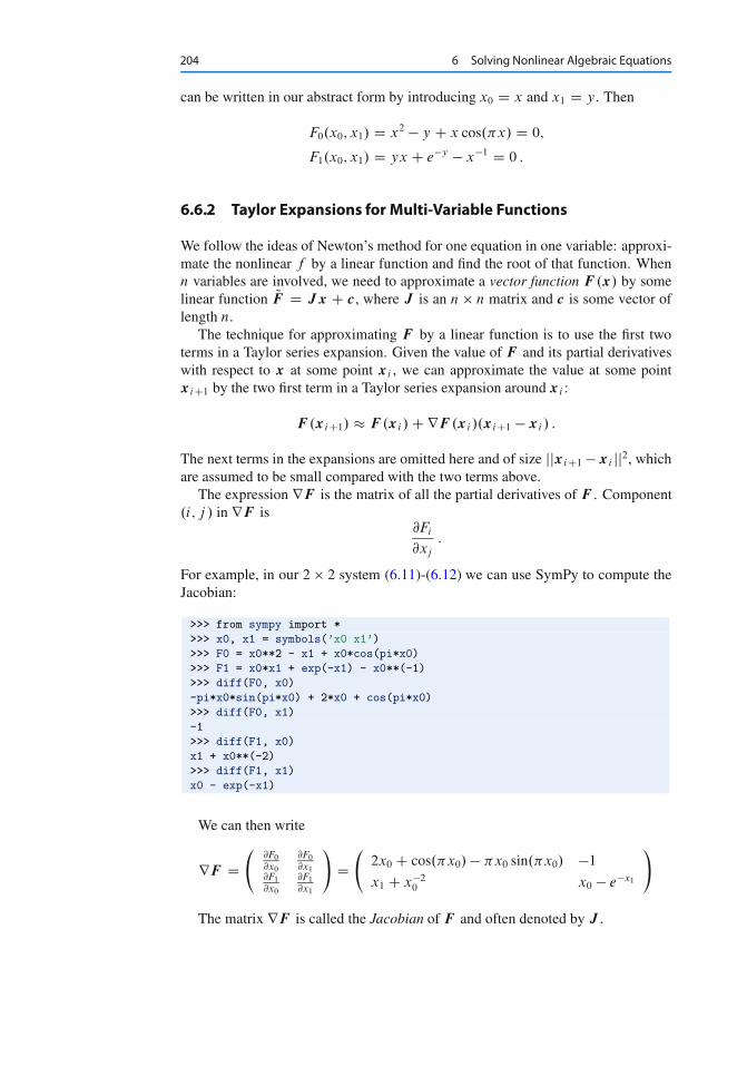
>>> from sympy import *
>>> x0, x1 = symbols(’x0 x1’)
>>> F0 = x0**2 - x1 + x0*cos(pi*x0)
>>> F1 = x0*x1 + exp(-x1) - x0**(-1)
>>> diff(F0, x0)
-pi*x0*sin(pi*x0) + 2*x0 + cos(pi*x0)
>>> diff(F0, x1)
-1
>>> diff(F1, x0)
x1 + x0**(-2)
>>> diff(F1, x1)
x0 - exp(-x1)
We can then write
rF D
@F0
@x0
@F0
@x1@F1
@x0
@F1
@x1
!D
2x0 C cos.�x0/ � �x0 sin.�x0/ �1
x1 C x�20 x0 � e�x1
!
The matrix rF is called the Jacobian of F and often denoted by J .
6.6 Solving Multiple Nonlinear Algebraic Equations 205
6.6.3 Newton’sMethod
The idea of Newton’s method is that we have some approximation xi to the root andseek a new (and hopefully better) approximation xiC1 by approximating F .xiC1/
by a linear function and solve the corresponding linear system of algebraic equa-tions. We approximate the nonlinear problem F .xiC1/ D 0 by the linear problem
F .xi / C J .xi /.xiC1 � xi / D 0; (6.13)
where J .xi / is just another notation for rF .xi /. The equation (6.13) is a linearsystem with coefficient matrix J and right-hand side vector F .xi /. We thereforewrite this system in the more familiar form
J .xi /ı D �F .xi /;
where we have introduce a symbol ı for the unknown vector xiC1 � xi that multi-plies the Jacobian J .
The i-th iteration of Newton’s method for systems of algebraic equations con-sists of two steps:
1. Solve the linear system J .xi /ı D �F .xi / with respect to ı.2. Set xiC1 D xi C ı.
Solving systems of linear equations must make use of appropriate software. Gaus-sian elimination is the most common, and in general the most robust, method forthis purpose. Python’s numpy package has a module linalg that interfaces thewell-known LAPACK package with high-quality and very well tested subroutinesfor linear algebra. The statement x = numpy.linalg.solve(A, b) solves a sys-tem Ax D b with a LAPACK method based on Gaussian elimination.
When nonlinear systems of algebraic equations arise from discretization of par-tial differential equations, the Jacobian is very often sparse, i.e., most of its elementsare zero. In such cases it is important to use algorithms that can take advantage ofthe many zeros. Gaussian elimination is then a slow method, and (much) fastermethods are based on iterative techniques.
6.6.4 Implementation
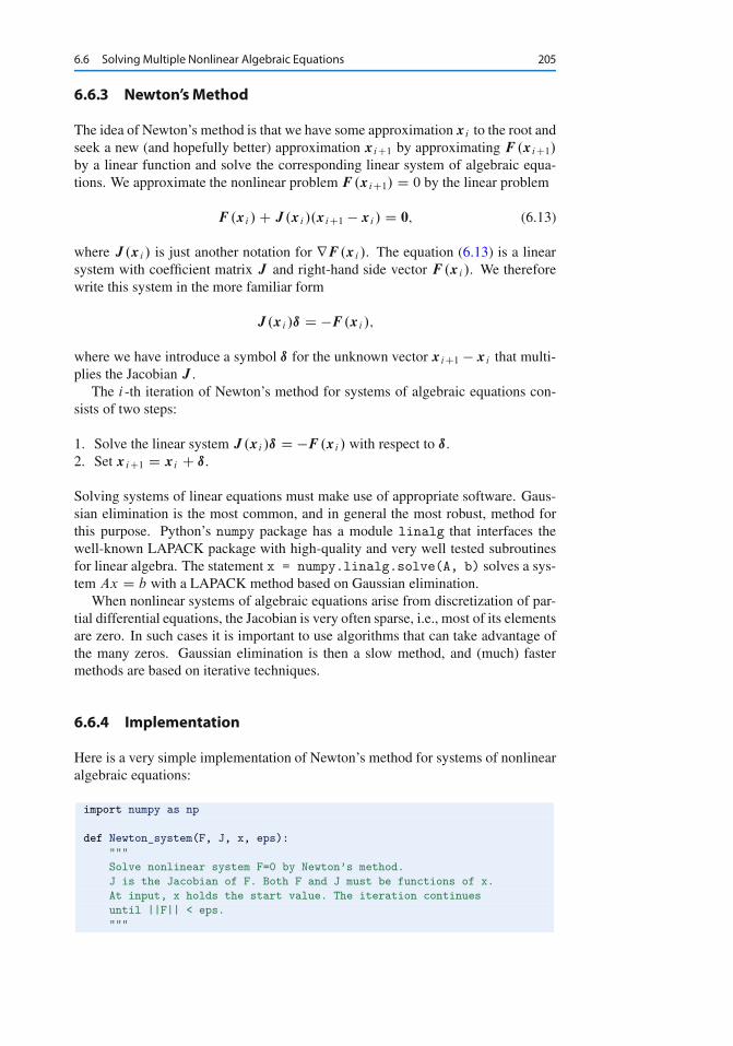
Here is a very simple implementation of Newton’s method for systems of nonlinearalgebraic equations:
import numpy as np
def Newton_system(F, J, x, eps):
"""
Solve nonlinear system F=0 by Newton’s method.
J is the Jacobian of F. Both F and J must be functions of x.
At input, x holds the start value. The iteration continues
until ||F|| < eps.
"""

206 6 Solving Nonlinear Algebraic Equations
F_value = F(x)
F_norm = np.linalg.norm(F_value, ord=2) # l2 norm of vector
iteration_counter = 0
while abs(F_norm) > eps and iteration_counter < 100:
delta = np.linalg.solve(J(x), -F_value)
x = x + delta
F_value = F(x)
F_norm = np.linalg.norm(F_value, ord=2)
iteration_counter += 1
# Here, either a solution is found, or too many iterations
if abs(F_norm) > eps:
iteration_counter = -1
return x, iteration_counter
We can test the function Newton_systemwith the 2 � 2 system (6.11)-(6.12):
def test_Newton_system1():
from numpy import cos, sin, pi, exp
def F(x):
return np.array(
[x[0]**2 - x[1] + x[0]*cos(pi*x[0]),
x[0]*x[1] + exp(-x[1]) - x[0]**(-1)])
def J(x):
return np.array(
[[2*x[0] + cos(pi*x[0]) - pi*x[0]*sin(pi*x[0]), -1],
[x[1] + x[0]**(-2), x[0] - exp(-x[1])]])
expected = np.array([1, 0])
tol = 1e-4
x, n = Newton_system(F, J, x=np.array([2, -1]), eps=0.0001)
print n, x
error_norm = np.linalg.norm(expected - x, ord=2)
assert error_norm < tol, ’norm of error =%g’ % error_norm
print ’norm of error =%g’ % error_norm
Here, the testing is based on the L2 norm of the error vector. Alternatively, wecould test against the values of x that the algorithm finds, with appropriate toler-ances. For example, as chosen for the error norm, if eps=0.0001, a tolerance of10�4 can be used for x[0] and x[1].
6.7 Exercises
Exercise 6.1: Understand why Newton’s method can failThe purpose of this exercise is to understand when Newton’s method works andfails. To this end, solve tanh x D 0 by Newton’s method and study the intermediatedetails of the algorithm. Start with x0 D 1:08. Plot the tangent in each iteration ofNewton’s method. Then repeat the calculations and the plotting when x0 D 1:09.Explain what you observe.Filename: Newton_failure.*.

6.7 Exercises 207
Exercise 6.2: See if the secant method failsDoes the secant method behave better than Newton’s method in the problem de-scribed in Exercise 6.1? Try the initial guesses
1. x0 D 1:08 and x1 D 1:09
2. x0 D 1:09 and x1 D 1:1
3. x0 D 1 and x1 D 2:3
4. x0 D 1 and x1 D 2:4
Filename: secant_failure.*.
Exercise 6.3: Understand why the bisection method cannot failSolve the same problem as in Exercise 6.1, using the bisection method, but let theinitial interval be Œ�5; 3�. Report how the interval containing the solution evolvesduring the iterations.Filename: bisection_nonfailure.*.
Exercise 6.4: Combine the bisection method with Newton’s methodAn attractive idea is to combine the reliability of the bisection method with thespeed of Newton’s method. Such a combination is implemented by running thebisection method until we have a narrow interval, and then switch to Newton’smethod for speed.
Write a function that implements this idea. Start with an interval Œa; b� andswitch to Newton’s method when the current interval in the bisection method isa fraction s of the initial interval (i.e., when the interval has length s.b � a/). Po-tential divergence of Newton’s method is still an issue, so if the approximate rootjumps out of the narrowed interval (where the solution is known to lie), one canswitch back to the bisection method. The value of s must be given as an argumentto the function, but it may have a default value of 0.1.
Try the new method on tanh.x/ D 0 with an initial interval Œ�10; 15�.Filename: bisection_Newton.py.
Exercise 6.5: Write a test function for Newton’s methodThe purpose of this function is to verify the implementation of Newton’s method inthe Newton function in the file nonlinear_solvers.py. Construct an algebraicequation and perform two iterations of Newton’s method by hand or with the aid ofSymPy. Find the corresponding size of jf .x/j and use this as value for eps whencalling Newton. The function should then also perform two iterations and return thesame approximation to the root as you calculated manually. Implement this idea fora unit test as a test function test_Newton().Filename: test_Newton.py.
Exercise 6.6: Solve nonlinear equation for a vibrating beamAn important engineering problem that arises in a lot of applications is the vibra-tions of a clamped beam where the other end is free. This problem can be analyzedanalytically, but the calculations boil down to solving the following nonlinear alge-braic equation:
coshˇ cosˇ D �1;

208 6 Solving Nonlinear Algebraic Equations
where ˇ is related to important beam parameters through
ˇ4 D !2 %A
EI;
where % is the density of the beam, A is the area of the cross section, E is Young’smodulus, and I is the moment of the inertia of the cross section. The most importantparameter of interest is !, which is the frequency of the beam. We want to computethe frequencies of a vibrating steel beam with a rectangular cross section havingwidth b D 25 mm and height h D 8 mm. The density of steel is 7850 kg/m3, andE D 2�1011 Pa. The moment of inertia of a rectangular cross section is I D bh3=12.
a) Plot the equation to be solved so that one can inspect where the zero crossingsoccur.
Hint When writing the equation as f .ˇ/ D 0, the f function increases its ampli-tude dramatically with ˇ. It is therefore wise to look at an equation with dampedamplitude, g.ˇ/ D e�ˇf .ˇ/ D 0. Plot g instead.
b) Compute the first three frequencies.
Filename: beam_vib.py.
Open Access This chapter is distributed under the terms of the Creative Commons Attribution-NonCommercial 4.0 International License (http://creativecommons.org/licenses/by-nc/4.0/),which permits any noncommercial use, duplication, adaptation, distribution and reproductionin any medium or format, as long as you give appropriate credit to the original author(s) and thesource, a link is provided to the Creative Commons license and any changes made are indicated.
The images or other third party material in this chapter are included in the work’s CreativeCommons license, unless indicated otherwise in the credit line; if such material is not includedin the work’s Creative Commons license and the respective action is not permitted by statutoryregulation, users will need to obtain permission from the license holder to duplicate, adapt orreproduce the material.