Embed Size (px)
Citation preview
STOCKHOLM SCHOOL OF ECONOMICS
Department of Finance
649 Degree Project in Finance
Spring 2017
Solving the Swedish Muni Puzzle – Piece By Piece
An analysis of liquidity premiums in the unique bond market of Sweden
Oscar Küntzel, 23324
John-Edward Olingsberg, 23323
ABSTRACT
This paper examines whether liquidity premiums can explain the Swedish muni puzzle. The Swedish
institutional climate presents a unique setting where default risk and taxes are equivalent in the
context of municipal and treasury bonds. Despite these similarities, we show that their yields still
differ substantially from one another after adjusting for coupons, peaking at as high as 178 basis
points during the depths of the European sovereign debt crisis. Operationalizing liquidity as
proportional bid-ask spreads, we construct measures of contemporaneous and future liquidity and
examine their explanatory power in the context of the Swedish muni puzzle. Adjusting for days to
maturity and orthogonalizing contemporaneous liquidity relative to future liquidity, we show that
differences in contemporaneous liquidity between municipal and treasury bonds can help explain the
muni puzzle. The results are statistically significant on the 1 percent level using two different types of
panel correlation methods. We find a significant constant of approximately 20 basis points which
cannot be explained by any of the mainstream explanatory variables typical to the muni puzzle.
SUPERVISOR: Irina Zviadadze
JEL CLASSIFICATION CODES: G12, G23, H74, H81
KEYWORDS: The Muni Puzzle, Bond Yields, Liquidity, Bid-Ask Spread
ACKNOWLEDGEMENTS: First and foremost, we would like to extend our sincere gratitude to our tutor Irina
Zviadadze for her helpful input over the course of the project. Further, we thank Mattias Bokenblom and Tobias
Landström at KommunInvest for highly insightful discussions and access to their Bloomberg terminals. Equally, we
would like to thank Professor Per–Olov Edlund for providing insightful information on relevant econometric issues.
Lastly, we extend our warmest thanks to Ida Metsis and Laura Lindberg who have consistently helped us throughout the
course of this paper.
Solving the Swedish Muni Puzzle – Piece By Piece Küntzel & Olingsberg
0
Stockholm School of Economics
TABLE OF CONTENTS
I. INTRODUCTION.................................................................................................................................................... 1
...................................................................................................................................................................................................
II. LITERATURE REVIEW ........................................................................................................................................ 4
2.1 Introduction ......................................................................................................................................... 4
2.2 Literature Survey .................................................................................................................................. 5
2.3 Theoretical Framework ........................................................................................................................ 14
III. RESEARCH DESIGN ........................................................................................................................................... 16
3.1 Problematization, Purpose & Contribution ........................................................................................... 16
3.3 Scientific Perspective .......................................................................................................................... 17
3.4 Method ............................................................................................................................................... 18
3.5 Empirical & Ethical Reflections ........................................................................................................... 21
IV. ANALYSIS & FINDINGS ..................................................................................................................................... 22
4.1 Summary of the Difference in ASW Yields for Municipal and Treasury Bonds .................................... 22
4.2 Describing the Variables and Our Panel Data ...................................................................................... 26
4.3 Examining the Presence of and Adjusting for Heteroscedasticity and Autocorrelation ........................... 28
4.4 The Basic Regressions ........................................................................................................................ 29
4.5 Contemporaneous and Future Liquidity - is Current Liquidity Just a Proxy for Future Liquidity? 31
4.6 Time and Contemporaneous Liquidity - Is Liquidity Just Capturing the Time Effect? 33
4.7 Relating the Results to the Muni Puzzle 37
4.8 Concluding Remarks ........................................................................................................................... 38
V. DISCUSSION & CRITICAL REFLECTIONS .................................................................................................... 38
5.1 Connecting the Findings to Theory ...................................................................................................... 38
5.2 The Research Question in a Broader Sense .......................................................................................... 39
5.3 Knowledge Contribution and Implications for Policymakers 40
5.4 Future Research .................................................................................................................................. 40
VI. LIMITATIONS OF RESEARCH ......................................................................................................................... 41
6.1 Data .................................................................................................................................................... 41
6.2 Models ................................................................................................................................................ 42
VII. CONCLUSION ..................................................................................................................................................... 43
REFERENCE LIST .............................................................................................................................................. 45
....................................................................................................................................................................................

Solving the Swedish Muni Puzzle – Piece By Piece Küntzel & Olingsberg
1
Stockholm School of Economics
I. Introduction
Since Modigliani and Miller’s (1958) defining piece on capital costs and the tax advantages of debt,
corporate taxes and leverage have occupied an increasing space in financial literature. Set aside the
direct implications that continue to characterize investment theory, capital budgeting and corporate
financing today1, tax-shields have come to occupy a growing proportion of related financial research.
Miller’s (1977) retort in the wake of a growing body of counterbalancing debt drawbacks published
by other authors suggests that tax exempt bonds of comparable characteristics should earn the same
after-tax yield as their taxable counterpart. As Chalmers (1998) is quick to point out, however, the
declining US term structure of implied tax rates between comparable municipal and government
bonds is not precipitated on default risk or call options. Affectionately termed the muni puzzle, the
phenomenon where long-term tax exempt municipal bond yields have outperformed that of their
long-term taxable government-issued equivalents has received several decades of research attention.
Prospective hypotheses for said after-tax yield differences have included, to name a few, institutional
tax profiles and the municipal bond market’s money tightness (FORTUNE, 1973), intertemporal tax
timing options (Constantinides and Ingersoll, 1982), systematic risk (Chalmers, 2006) and municipal
market segmentation by maturity (Kidwell and Koch, 1983). The latter is closely echoed by a corpus
of divided literature on the importance of commercial banks’ vested interest in short-term
securities2. These credit institutions have, historically, accounted for a considerable portion of the
US municipal market (ibid). In light of the maturity matching principle, commercial banks tend to
favor short-term municipal bonds in lieu of their longer equivalents due to their liabilities’ short
average maturity. Further, municipals’ tax savings look favorably to commercial banks as opposed to
taxable government bonds given their often-high tax brackets vis-à-vis other financial intermediaries.
Under these premises, long-term and short-term municipal bonds are imperfect substitutes, and thus
attract different institutional investors. In this vein, commercial banks’ short-term preferences elicit a
demand-driven upward bias in long-term municipal yields compared to long-term government
bonds.
1 See, for instance, Graham and Rogers’s (2002) discussion on the impact of hedging on capital structure due to tax convexity and incentives, or Korteweg’s (2010) findings on the optimal leverage ratio based on firm characteristics including corporate profitability and size. 2 Compare, for instance, Campbell’s (1980) discourse on the lackluster empirical significance of municipal maturity segmentation with that of Hendershott and Kidwell’s (1978) findings between nationally and regionally marketed municipal bonds.

Solving the Swedish Muni Puzzle – Piece By Piece Küntzel & Olingsberg
2
Stockholm School of Economics
Despite these efforts, attempts at reconciling theories for the downward bias in long-term
government bond yields have been largely unsuccessful (Liu et al., 2003). In an especially notable
paper, Liu et al. (2003) anatomize the muni puzzle and find robust evidence for default and liquidity
risk premiums in AAA, AA/A and BBB rated municipal bonds. Incorporating these explanatory
variables dissipates much of the US term structure’s municipal-government implicit tax rate, thus
resolving much of the muni puzzle. Nevertheless, the deterministic role of liquidity in unravelling
the muni puzzle has received a strong empirical footing whilst that of credit risk has proved less
consistent. Fontaine and Garcia (2014) find liquidity premiums explain a significant portion of
Treasury bonds’ risk premium, Chen et al. (2007) account for as much as half the cross-sectional
variation of yield spreads in corporate investment grade and junk bonds via liquidity measures and
Liu et al. (2003) extend this result to investment grade municipal bond yields. Indeed, scholars by
and far recognize liquidity as a meaningful and informative determinant of differing municipal and
government after-tax bond yields. In spite of this, a plenitude of disparate liquidity metrics continues
to occupy the liquidity literature space, making its many operationalization’s less consistent than its
generally agreed-upon importance as an explanatory variable to the muni puzzle3. With respect to
default risk, Trzcinka (1982) observes that credit exposure accounts for much of the after-tax yield
differential accentuated by Miller (1977), Yawitz et al. (1985) attribute their fourfold higher
difference in yield spreads between prime-rated munis4 and treasuries compared to prime- and
medium-rated municipal bonds to credit risk premiums. E contrario, Ang et al. (1985) and Chalmers
(1998) both contest the muni puzzle remains unexplained after allowing for credit rating
discrepancies.
Credit risk’s inconsistent explanatory power in the muni puzzle may serve as an impasse for
the muni-treasury researcher. The Swedish institutional climate serves as a compelling instance
where such a predicament is, by and large, avoided. Indeed, for over a decade more than half of
Sweden’s municipalities have collaborated under a joint inter-municipal structure coined
KommunInvest (the Swedish Local Government Debt Office)5 in 1986 (KommunInvest, 2017). This
organizational cooperative came to fruition as a bargaining vessel for improved collective borrowing
terms and access to capital markets in meeting, primarily, Sweden’s municipal infrastructural needs.
By the close of 2016, the institution represented some odd 275 municipalities6 and managed 277
3 See, for instance, Aitken and Carole (2003) for an insightful discussion on the multifaceted ways of measuring liquidity. 4 The term “muni(s)” is used interchangeably as an abbreviation for “municipal bond(s)” herein. 5 Abbreviated “KI” and “SLDO” henceforth. 6 Corresponding to ~ 94.8% of all Swedish municipal jurisdictions.
Solving the Swedish Muni Puzzle – Piece By Piece Küntzel & Olingsberg
3
Stockholm School of Economics
SEKbn in issued bonds, analogous to ~48% of all local government loan financing (KommunInvest
2017). In 2006 KI received a AAA rating from Standard & Poor’s, having held an Aaa equivalent
from Moody’s since 2002, making it Sweden’s sole organization with triple-A/a ratings from both
credit rating agencies and - more importantly - of comparable credit risk to Riksgälden (the Swedish
National Debt Office)7: the legal issuer of Swedish government bonds (KommunInvest, 2017).
Moreover, RiGä and KI are constitutionally-defined legal equivalents such that the latter cannot
declare insolvency or bankruptcy8 nor postpone payments unless the state itself defaults. In other
words, the state bears the ultimate fiscal responsibility for the local government sector
(KommunInvest, 2016). Further, legislative changes higher up the political hierarchy (i.e.
government-sanctioned altercations to local government) must be compensated for so as to
neutralize any financial effect to municipalities (Regeringskansliet, 1991). Local government
imbalances are, moreover, adjusted annually via cost and income equalization schemes
(Regeringskansliet, 2004). Swedish munis and treasuries are, therefore, indistinguishable with respect
to credit risk from the perspective of both de facto market ratings as well as legal
bankruptcies/probabilities of default. Akin to this train of thought9, there are no tax differences
characterizing the investor profiles of munis vis-à-vis Swedish government bonds.
The notion of pooling municipal financing has even prompted Ang and Green (2011) of the
Hamilton Project - an economic policy initiative comprised of academics, business leaders and
former public policy makers - to propose a shared non-profit organizational body (CommonMuni)
representing US municipal interests in an endeavor to lower borrowing costs by minimizing private
information and illiquidity. Lack of the latter, the authors purport, gives rise to ~$30bn in liquidity
costs alone. This institutional framework is described as an independent, non-profit advisory
disseminating information for the benefit of individual municipalities, states and other market
participants. In this light, KI is strikingly similar to the US proposed structure demarcating ongoing
politico-economic discussions within the municipal bond market, providing a pronounced context
for its study in a Swedish institutional context.
7 Abbreviated “RiGä” and “SNDO” henceforth. The SNDO retains a credit rating AAA/Aaa from Standard & Poor’s, Moody’s and Fitch respectively (Riksgälden, 2014). 8 Local government is not covered by the Swedish Bankruptcy Act. Swedish Court rulings have enforced this legal doctrine (Göta Hovrätt, 1994). 9 Pursuant to discussions with Mattias Bokenblom, Head of Research & Development, and Tobias Landström, Senior Funding Officer, of KI.
Solving the Swedish Muni Puzzle – Piece By Piece Küntzel & Olingsberg
4
Stockholm School of Economics
With the above in mind, this paper attempts to bridge the academic lapse in extant muni
puzzle literature by investigating a unique regulatory and institutional climate which supersedes
much of the clout that has typically surrounded (i) credit/default risk and (ii) tax differentials in a
traditionally US-dominated municipal versus government bond space. In doing so, this study can
highlight the less operationally understood liquidity risk in a rather homogenous
municipal/government bond environment. Further, this thesis also sheds light on a public proposal
area for policymakers to continue to develop - namely, the prospect of a shared organizational body
mediating the need for liquidity and information transparency in issuing munis.
With the research question “Can liquidity premiums explain the Swedish Muni Puzzle”, this
paper draws inspiration from Goldreich et al. (2005) who examined how differences in liquidity
measures between bonds can help explain differences in their yields. This research is to the best of
our knowledge the only study examining the muni puzzle in a setting where default-risk and tax
considerations can be safely ignored.
II. Literature Review
2.1 Introduction
As discussed in I. Introduction, examining the determinants of municipal bond yields has been of
interest to academics for the better part of forty years. At the time, Hastie (1972) shed light on the
differences discerning (specifically) municipal bond yields in the US by researching the effects of
variables such as default history, demographics and diversification. Today, researchers are more
particularly preoccupied with explaining why empirical data shows yields on long-term tax-exempt
municipal bonds that are higher than expected. This chapter is designed to familiarize the reader with all the theories and tools that have been
developed and effectively used by academics in their effort to explain bond pricing in general and,
through it, the muni puzzle. The 2.2 Literature survey section aims to make systematic assessments of
major literary areas based on extant research and draw key conclusions that lay the foundation for
our research. This survey, particularly 2.2.3 Liquidity, stretches beyond both the muni puzzle and
general bond market to give the reader a broad and fair view of relevant past findings. To bridge the
gap between past research and our research, 2.3 Theoretical framework identifies tools and approaches
from these studies that are most relevant to adopt given the distinct setting of this study.
Solving the Swedish Muni Puzzle – Piece By Piece Küntzel & Olingsberg
5
Stockholm School of Economics
2.2 Literature Survey
2.2.1 Taxes
When the muni puzzle has been discussed in the US, municipal bonds (tax-exempt) and government
bonds (taxable) have been compared to one another. Municipal bond yields have and continue to be
higher than one less the appropriate tax rate multiplied by the relevant government bond yields. In a
country where bond-income taxes do not differ on a municipal or federal level, like Sweden, the
comparison of munis and treasuries can be made without any correction for taxes. The implications
of taxes on bond yields, however, can be extended further than the plain vanilla tax-rate differentials
between US treasury and municipal bond yields when analyzing the muni puzzle. Longstaff (2011)
suggests there is a negative market risk premium on the marginal tax rate due to the federal income
system’s progressive taxation. Progressive taxes, it is argued, move investors to higher tax brackets in
economic booms, making after-tax coupon cash flows countercyclical. Resultantly, taxes’ negative
market risk premium make it a ‘systematic asset pricing factor’ increasing taxable government bond
returns which, by extension, diminishes the extent of the muni puzzle. This result stands in stark
contrast to Chalmers (2006), who described a “consumption risk” in the payoff timing of bond cash
flows. More specifically, muni-treasury payoffs from different taxes are thought to affect their yields
through the current marginal utility of consumption due to current economic conditions. Indeed,
one can hypothesize a government bond investor whose taxable cash flows become exceedingly
cumbersome in an economic context where the current marginal utility of consumption is high.
Nevertheless, his results showed that ‘systematic risk’, i.e. risks that had bond price effects due to
systematic correlations with consumption risk, were not likely to resolve the muni puzzle.
Generally speaking, taxes are often included in models that primarily examine other effects
like that of default or liquidity risk. Liu et al. (2003), for example, obtain implicit tax rates (after
taking default probabilities and liquidity risks into account) close to the statutory tax rates of
institutional investors and high-income individuals.
2.2.2 Credit Risk
Default/credit risk has withheld a long-lasting tradition of as a heavily researched academic
field, earning it wide acceptance as a fundamental determinant of bond yields. Yawitz et al. (1985)
pioneered the terrain by studying how default probabilities affect bond prices and consequently yield
spreads. More recent evidence for the relationship between bond yields and credit risk can be found
Solving the Swedish Muni Puzzle – Piece By Piece Küntzel & Olingsberg
6
Stockholm School of Economics
through the like of Norden and Weber (2007) and Gilchrist et al. (2009) who, through the bond
market, examine credit market shocks, economic activity and CDS spreads. More than a decade after Yawitz et al.’s (1985) paper, Chalmers (1998) found that the yields of
effectively default free government-secured bonds still were too high; despite credit risk’s consensus-
approval as a vital component of the muni puzzle, there remained other overlooked pieces of the
jigsaw. Subsequent research has converged to incorporate default risk in a broader context of
determinants in analyzing the muni puzzle. Several of these are discussed in 2.2.3 Liquidity. On a technical note, in isolating the risky characteristics of bonds researchers tend to
reconstruct their yields into common, comparable metrics. Their intent is to strip out the shared,
risk-free component of bond yields while making corrections for other effects that may impact the
yield. Several of these otherwise extensive corrections can today be made conveniently through
programs like Bloomberg or Thomson Reuters. 2.2.3 Liquidity
Liquidity is continuously priced throughout security markets. In the 1980s, Amihud and Mendelson
(1986) demonstrated bid-ask spreads affect assets’ expected returns. Later, Boudukh and Whitelaw
(1993) showed that government bond prices depend on short sell constraints, echoing Vayanos’s
(1998) findings that transaction costs give rise to liquidity rebates in the form of lower bond prices
and, hence, higher expected returns. Though the price of liquidity is ever-present across practically
all asset classes (equities, treasury bonds/bills, municipal bonds, corporate bonds and so forth), there
is no universally accepted way to measure or operationalize liquidity. As Goldreich et al. (2005, p.1)
articulated, “[…] the notion of liquidity itself is hard to pin down”. Both within and across security
markets, therefore, research areas have differed widely in their methods for capturing the
quintessential dynamics of liquidity. Compare, for instance, Viral et al. (2004) who made use of a
liquidity-adjusted CAPM in examining ‘liquidity commonality’, with Goldreich et al.’s (2005) paper
that examined forward-looking liquidity measures through pairs of on-the-run (i.e. most recently
issued) and off-the-run bonds. Further, as Houweling et al.’s (2004) review of liquidity proxies
demonstrates, the empirical literature’s findings regarding the impact of liquidity on bond yields has
often been multifaceted and even conflicting. More recently, Choudhry (2010) highlighted that
individual proxies of liquidity are rarely satisfactory and often incomparable across markets. It is
therefore hardly surprising that, as previously alluded to, past researchers have historically used a
variety of measures in capturing the mechanics of liquidity (Aitken and Comerton-Forde, 2003).
Solving the Swedish Muni Puzzle – Piece By Piece Küntzel & Olingsberg
7
Stockholm School of Economics
Indeed, just a meager twenty years ago the corpus of literature used at least 68 measures of liquidity
(Aitken and Winn, 1997). Broadly speaking, when liquidity in bond and equity markets has been scrutinized, its measures
have been categorized as either of direct or indirect nature (Houweling et al., 2005). Direct metrics
tend to pertain to transactional data but have included variants of high-frequency order-based data,
while indirect measures capture some general characteristic of the bond and/or end-of-day prices.
As the extant research regularly bears witness to, however, that which separates indirect and direct
operationalizations of liquidity has been somewhat elusive. Nevertheless, examples classic to
transactional (i.e. direct) data have included quoted and effective bid-ask spreads, quoted and traded
volumes and trading frequency (ibid). The choice of measure used is however, as is often the case,
delimited by a combination of data availability, the researcher's view on liquidity and his/her
research objectives. With that said, direct measures are generally considered closer to the
fundamental essence of liquidity insofar as they are directly relatable to investors’ economic
experiences when converting cash to assets and vice versa. For instance, in any given transaction at
any given moment, investors customarily incur liquidity costs in the form of the de facto spread in a
buy and sell order. Investors are, concurrently, transactionally limited by the current order volumes
available in each of the buy and sell legs, i.e. the order book depth and size. With respect to indirect
measures, these are commonly used to represent direct measures when direct measures are
unavailable. Some sixty years ago, Fisher (1959) used the indirect measure issued amount of a bond as
a proxy for trading volume - a direct measure of liquidity. This measure continues to be used in
modern literature by authors such as Houweling et al. (2005), and has been reproduced together
with other proxies like age/tenor and yield volatility (see, for instance, Sarig and Warga (1989) and
Hong and Warga (2000)). Perhaps a more evident systematization, measures can on top of being direct or indirect be
trade- or order-based. In an effort to provide some clarity as to which of these are more accurate
proxies for liquidity, Aitken et al. (2003) researched the differences between trade- and order based
liquidity metrics for stocks. These, it was found, often yield completely different research results,
wherefore order-based measures were concluded to be superior when examining the economic
crisis’s impact on the Indonesia Stock Exchange (previously the Jakarta Stock Exchange). Arguing
that the ability to instantaneously convert cash into securities at a minimum cost (and vice versa) is
the core of liquidity, the authors purported that ex post transaction measures like monthly turnover
Solving the Swedish Muni Puzzle – Piece By Piece Küntzel & Olingsberg
8
Stockholm School of Economics
(i.e. trade-based measures) are inferior to ex ante order-based operationalizations including bid-ask
spreads and order book depth.
2.2.3.1 Liquidity and Transaction Costs
At this juncture, it is necessary to explain the relationship between transaction costs and liquidity and
why measurements based on spreads are widely used when measuring liquidity risk. In doing so, it is
required to grasp how different areas of research categorize these concepts depending on the
implicit research question being examined. As previously mentioned, Houweling et al. (2005)
classified bid-ask spreads (a transaction cost) as a type of direct measure of liquidity. When
transaction costs themselves are the chief research focus, however, the literature categorizes
transaction costs as explicit or implicit (Aitken and Comerton-Forde, 2003). Explicit transaction costs
have come to include commission costs and taxes, and lie outside of the control of the relevant
exchange. Their implicit equivalents have included the bid-ask spread and various opportunity costs,
and are often directly related to structural marketplace characteristics like short sell constraints.
Marketplaces and exchanges often possess some inherent ability to change these implicit costs by
altering technology, instrumentation and regulation (ibid). This strain of literature defines bid-ask
spreads as a type of implicit transaction cost10; an investor must incur the cost of the bid-ask spread
if they wish to trade in the market, and in doing so they are subject to explicit costs like taxes. By
simple virtue of our intuition, higher transaction costs imply lower market liquidity. Recalling the
discussion on direct and indirect measures of liquidity, the preferred direct measures (e.g. bid-ask
spreads, in this case) should, logically, capture the relevant costs associated with trading. The
literature thus gets ambiguous when bid-ask spreads are included as just one type of transaction cost,
on the one hand, yet is presupposed to encompass said transaction costs on the other. Phrased
differently, are transaction costs measures of liquidity, or liquidity measures of transaction costs?
This obscurity can come across as a source of confusion to the uninformed reader and we are
reminded of Goldreich et al.’s (2005, p.1) foreboding “the notion of liquidity itself is hard to pin
down”. In this paper, which of the preceding cause-and-effect interpretations of liquidity and
transaction costs is the most relevant is not discussed in greater detail. The key takeaways are that
10 This literary body has focused on the origins of illiquidity and is often referred to as market microstructure research. This field of inquiry looks into different forms of bid-ask spreads and ‘market impacts’ (i.e. the costs that investors incur when driving up (down) prices with large buy (sell) quantities passed the best ask (best bid)), and the characteristics of exchanges and marketplaces giving rise to these.

Solving the Swedish Muni Puzzle – Piece By Piece Küntzel & Olingsberg
9
Stockholm School of Economics
transaction costs (i) can be explicit or implicit, (ii) correlate with how markets and exchanges operate
in general, and (iii) are highly interconnected with bid-ask spreads. Liquidity proxies, in turn, capture
general views of market liquidity effectively when seen as costs that investors must incur to trade in
markets. Nonetheless, as Archarya et al. (2004) explicated, liquidity is (unfortunately) not an
observable variable and consequently tangible measures such as the bid-ask spread are used as
substitutes. Amihud and Mendelson (1986, p.1) voiced a similar train of thought when stating that
the bid-ask spread is the sum of the buying premium and the selling concession, making it a “natural
measure of liquidity”. Amihud et al. (2006, p. 270), later expressed liquidity should simply be thought
of as “the ease of trading a security”.
2.2.3.2 Validity of Liquidity Proxies
In covering different geographical markets over elongated periods of time, research on liquidity has
periodically been forced to compromise on the use of direct measures. So much so, that creating
proxies from daily data and bond characteristics (i.e. making use of indirect measures) to reach
valuable conclusions has become commonplace to almost all markets set aside the US treasury
market, which has been demarcated by a relative abundance of information (Houweling et al.,
2005). A highly influential paper by Goyenko et al. (2009) speaks to this liquidity measure
concession when explaining how daily return and volume data often are used to design liquidity
measures proxying investors’ ‘true’ intra-day liquidity/transaction costs. In doing so, the authors
examined the underlying assumption that transaction costs are captured by readily available proxies.
When liquidity proxies are not directly connected to direct measures, the authors reasoned that
consensus of the validity of indirect measures will differ substantially, driving their hypothesis that
the latter measures do not accurately mirror investors’ experiences when trading securities. Contrary
to their ex ante beliefs, the paper found that that low-frequency measures performed surprisingly
well in estimating high-frequency direct measures. Further, it was deduced that more detailed, high-
frequency data was often simply not worth the time and effort it required. The measures most apt
and relevant to the research at hand will, however, depend on the specific area under study. With
respect to this paper, 2.3 Theoretical Framework discusses the empirical selection of liquidity proxies
considering the recent research of Goyenko et al. (2009), who, like Aitken et al. (2003), collectively
Solving the Swedish Muni Puzzle – Piece By Piece Küntzel & Olingsberg
10
Stockholm School of Economics
determine that order-based data, as opposed to trade-based data, is superior when creating liquidity
benchmarks11. The reader should at this point be familiarized with (i) a broad view of the type of
measurements that are used in liquidity-related research (ii) how liquidity measures can be
categorized/interpreted and (iii) liquidity measures’ relative research appropriateness. Below follows
a brief discussion on some of the main results and models used within the concepts commonality,
on-the-run/off-the-run treasury bonds, current and future liquidity as well as the role of investment
horizons on yields.
2.2.3.3 Liquidity and Commonality
Peter and Stamboughs (2003) showed that expected returns on stocks are cross-sectionally related to
how sensitive the individual assets are to market wide, aggregate liquidity (i.e. liquidity commonality).
From data stretching over a period of thirty-four years, they concluded that (after adjusting for
aspects like size, momentum, value and market return sensitivity) the average return on high liquidity
sensitive stocks was 7.5 percent higher than that of low liquidity sensitive stocks. The majority of the
various areas within liquidity research are covered in the equities literature12. As the above Peter and
Stamboughs (2003) example indicates, liquidity commonality is no exception. A growing corpus of
evidence, however, has been presented in extant bond and non-equities literature13 which asserts that
assets are, in general, exposed to the phenomenon of market wide liquidity, reflected in underlying
prices.
It would seem, therefore, that the working consensus is that exposure to market liquidity is
reflected in most if not all financial markets’ prices. With that said, liquidity risk per se is far from the
only way liquidity affects asset pricing. Importantly, the absolute level of liquidity is also an actively
priced component of the wider market liquidity/liquidity commonality (Amihud et al., 2006).
Previously mentioned Chen et al. (2007) employed cross-sectional liquidity levels in accounting for
as much as half of the cross-sectional variation of investment-grade and speculative-grade bond yield
11 Effective and realized spreads as well as price impacts are calculated using TAQ and Rule 605 data. Rule 605 data is said to be better for several reasons. For example, the midpoint is taken at the time of receipt (not execution), i.e. Rule 605 data allows for order-based rather than trade-based data. 12 See, for example, Huberman and Halka (2001) and Hasbrouck and Seppi (2001). 13 See, for example, Beber et al. (2009), Lin et al. (2011) and Geanakoplos (2003) for insights on the liquidity commonality of sovereign bonds, corporate bonds and the holistic financial system, respectively.
Solving the Swedish Muni Puzzle – Piece By Piece Küntzel & Olingsberg
11
Stockholm School of Economics
spreads. Moreover, scholars contend that risk-averse investors are compensated for not just the lack
of ease of trading today, but equally the riskiness of potential future liquidity, as the below elaborates.
2.2.3.4 Current and Future Liquidity, and on-, off-the-run Bonds
A bond is on-the-run if it was the most recently issued in a series of periodically issued securities. All
other bonds are, hence, off-the-run. On-the-run bonds are primarily discussed when analyzing
treasuries, particularly US treasuries14, but are also relevant for other bond types when researching
liquidity (see the previously discussed Houweling et al. (2005)). Whichever the case, ‘on-the-run’ and
‘off-the-run’ have become salient bond classifications due to their substantially different liquidity
characteristics. Specifically, the former is considerably more liquid as it earns more trading interest,
frequency and volume. US treasury notes are issued on a rolling basis, auctioned every month and
mature after two years - hence, there are consistently twenty-four two-year treasury notes
outstanding. Goldreich et al. (2005) used this predictability to determine whether future liquidity was
being priced using a total of seven different liquidity measures. Fourteen years prior, Amihud and
Mendelson (1991) maintained that liquidity-related costs are incurred several times during the life of
an asset, such that the present value of liquidity costs ultimately determines in what manner asset
prices ought to be affected by liquidity. Goldreich et al.’s (2005) obtained results were paramount to
the literary body of liquidity and bond yields. Briefly, they evidenced (i) exact measures and statistical
interpretations explaining differences in liquidity between on-the-run and off-the-run bonds, (ii)
further insight into the relative explanatory powers of different proxies for liquidity, and (iii) that
investors price not only contemporaneous/current liquidity (i.e. liquidity today), but also future liquidity.
2.2.3.5 Liquidity and Investment Horizons
Yet another branch of liquidity worth noting is the effect of investment horizons on the costs to
investors, and thus their (net) return of holding the asset. Amihud and Mendelson (1991) elucidated
that a short horizon implies an investor ought to hold a more liquid asset or risk transaction costs
exhausting all returns. A long investment horizon, as the authors would have it, suggests holding an
illiquid asset as the net return is boasted by liquidity costs that are never actually incurred. These
investment horizon dynamics are reducible to two distinct investor-groups; those with long, and
those with short investment horizons. This categorization has become known as a type of clientele
14 See, for example, Pasquariello and Paolo (2009) and Goyenko et al. (2009).

Solving the Swedish Muni Puzzle – Piece By Piece Küntzel & Olingsberg
12
Stockholm School of Economics
effect. By consequence, non-linear relationships are thought to exist between liquidity and returns
(Amihud and Mendelson, 1986).
2.2.3.6 Liquidity vs Default Risk Researchers have devoted a substantial amount of time and effort in explaining the relative
importance of liquidity and default risk, as well as the circumstances where one matters more than
the other. Their interaction and dependence on factors including macroeconomic conditions and
financial distress have also been subject to much deliberation. Beber et al. (2009) show that at
different times and for different reasons, credit quality and liquidity are both demanded by investors.
As Codogno et al. (2003) suggested six years prior, Beber et al. (2009) support the notion that
European sovereign yield spreads are primarily driven by credit quality. In low credit countries,
however, the authors convincingly demonstrated that the concern for liquidity outweighs that of
credit quality. Moreover, in times of market distress, cash flows are typically seen as chasing liquidity,
i.e. there is a flight-to-liquidity, not a flight-to-quality (ibid). Liquidity also stands as the most
important determinant when the bond market is exposed to sizeable capital in- or outflows,
accounting for the lion’s share of sovereign yield spreads. This is an especially powerful result since
past research by Ericsson and Renault (2006) previously presented evidence that, in the US
corporate bond market, credit quality and liquidity were positively correlated, which has complicated
the separation of the two concepts. Bao et al. (2011, p.911) found similar results as Beber et al. (2009) by examining US corporate
bonds between 2003 and 2009, and concluded that there is a “strong link between bond illiquidity
and bond prices”. Even for AAA-rated bonds, illiquidity on a market level affects bond yield
variation over time, dwarfing the credit risk component. This result both supports and contests the
research of Longstaff et al. (2005), who used the credit default swap market to examine the relative
importance of credit and other risk classes, principally liquidity risk. The component of the yield
spread not due to credit risk was, both papers found, shown to be time varying and related to bond-
specific-15 as well as macro-liquidity measures in the bond market. At the same time, Longstaff et al.
(2005) attributed most the observed yield spread (51%) of AAA/AA-rated bonds to credit risk.
15 These included, among others, bid-ask spreads, accessibility to the bond issue in the market and the age of the bond.
Solving the Swedish Muni Puzzle – Piece By Piece Küntzel & Olingsberg
13
Stockholm School of Economics
2.2.4 Interest Rate Risk
Discussing interest rate risk for treasury and municipal bonds may, at first, seem somewhat odd
given their latent relationship to the bond market. On that note, however, given that the yield curve
can look different at different times, and is delimited by some form of non-linear shape across
maturities (Chan et al. 1992, Duffee 2002), there is an innate risk in holding bonds with different
maturities or positions on the yield curve. In the literary body, the discrepancy of time itself and the
risk that comes with it is often adjusted using (i) some variant of interpolation between known yields
at different maturities16, (ii) some version of hypothetical security yield comparison17 (iii) and/or
assumptions that can justify not making any corrections due, in large part, to almost identical
maturity dates.
2.2.5 Underwriter Reputation
Another perhaps less obvious and less quantifiable aspect to consider when analyzing bond prices
and the muni puzzle is that of the underwriter’s reputation. In the US, municipal bonds have over
time seen higher issuance prices afforded by larger and more prestigious underwriters (Daniels and
Vijayakumar, 2007). Their stronger reputational backing, it is argued, promotes less information
asymmetry between issuers and borrowers, augmenting said issue prices (ibid). Fang (2005) echoed
this prospect by documenting lower earned yields in issues from reputable banks. Despite higher
fees, he contends, the issuer’s net proceeds increase. This phenomenon is most pronounced in
speculative grade bonds. Put simply, underwritings from reputable banks signal high issue quality
(ibid).
2.2.6 Investor Attention
Investors, like all people, have a finite information processing ability under a certain period of time,
i.e. limited attention. Akin to underwriter reputation, this is a somewhat less defined area than many
more tangible determinants of bond yields. Psychological studies examining investor attention are
vast and can, for a rather comprehensive reading, be explored through the reviews of Khaneman
(1972) as well as Pashler and Johnston (1998).
Due to this inherent human limitation, investors have been shown to first focus on, and
process, market-level information when market-wide uncertainty has suddenly increased. Only once
16 See, for example, Amihud and Mendelson’s (1991) linear weighted scheme. 17 Goldreich et al. (2005) elegantly implemented this correction.
Solving the Swedish Muni Puzzle – Piece By Piece Küntzel & Olingsberg
14
Stockholm School of Economics
this is done, are investor resources dedicated to idiosyncratic information of interest. This is a
(relatively) short-term phenomenon and takes less than 10 days to complete (Peng et al., 2007).
Nevertheless, investor attention is exceedingly hard to measure. The rise of information technology
has made data collection pertaining to investor behavior more transparent and quantifiable,
producing new operationalized measures of investor attention such as the google search frequency
measure “Search Volume Index” (SVI). An increase in the SVI metric is consistently correlated with
higher first day returns in the event of an IPO, followed by a subsequent underperformance in the
long-run (Da et al., 2011). Further, investor attention research often questions rational investor
models. For example, processing more sector-wide than firm-specific information (coined category-
learning behavior) coupled with investor overconfidence creates return co-movement characteristics in
the market that cannot be explained by models based upon agents acting completely rationally (Peng
and Xiong, 2006).
2.3 Theoretical Framework
Even though all research discussed in the literature review is relevant for the understanding of the
issues raised in this paper, the theoretical framework aims at using the literature review as a
backdrop to establish what past studied areas are closest to and most applicable for the empirical
process and setting of this study. The literature narrows down substantially for three reasons: (i) it is
simply not possible to examine all aspects that can possibly influence bond yields, (ii) the muni
puzzle can, in Sweden, be examined from a perspective where several factors are naturally
eliminated, and (iii) scarce data availability has constrained the possibility of using other albeit less
robust variables from past research.
2.3.1 Taxes
Even though taxes play a significant role when examining the muni puzzle in the US, the fact that
municipal bonds are not tax exempt in Sweden eliminates any need for tax-rate adjustments. Neither
is there any need to discuss negative market risk premiums or systematic correlations with
consumption risk as discussed through Longstaff (2011) and Chalmers (2006).
2.3.2 Credit Risk
Analogous to taxes, there is little doubt that credit/default risks are actively at work in the muni
puzzle. In the Swedish institutional climate, however, both KI and RiGä have identical credit ratings

Solving the Swedish Muni Puzzle – Piece By Piece Küntzel & Olingsberg
15
Stockholm School of Economics
in the bond market and, more importantly, are constitutional equivalents. Moreover, RiGä has taken
upon itself a statutory role comparable to ‘lender of last resort’ in the unlikely event of KI’s
insolvency - in other words, KI cannot default without RiGä doing so. KI is, in the same vein,
unable to declare bankruptcy due to its municipal representation. Consequently, no specific model
incorporating credit risk is used herein.
2.3.3 Liquidity
The bulk of previous research that lays the foundation to this paper is liquidity-related. Indeed,
liquidity appears as the most promising contender in explaining the Swedish muni puzzle given the
absence of tax and credit differentials between munis and treasuries. In selectively choosing the most
relevant research to incorporate and build upon, certain papers are naturally more suitable than
others given the field’s rather extensive coverage of different asset classes, markets and methods18.
Combining the limited data available for the purposes of this study with the historically exuberant
amount of liquidity measures (Aitken and Winn, 1997) of different validities (Houweling et al., 2005,
Goldreich et al., 2005), it is crucial that a relevant, economically relatable measure is chosen that
accurately portrays investors’ experienced liquidity costs.
Drawing on mainstream conclusions shared by the better part of extant research19, the
analytical approach and the liquidity measure should capture the level of liquidity today and be
receptive to the eventuality of a forward-looking investor realizing the implications of incurring
costs relating to trading an asset over time. Moreover, learning from the results of Goyenko et al.
(2009) and Aitken et al. (2003), order-based results are generally superior to trade-based measures.
Direct measures are furthermore seen as preferable in liquidity research. Recall, however, Goyenko
et al.’s (2009) study that demonstrated low-frequency end-of-day data (or even monthly or yearly
data) performs practically as effectively as high-frequency equivalents. Finally, Bao et al. (2011) and
Amihud and Mendelson (1991) showed that liquidity is properly modeled when changes in measures
of indirect and direct costs give rise to changes in bond prices and, by extension, yields.
Goldreich et al. (2005) is a considerable source of inspiration to this paper for two principal
reasons. First, their research provides an intuitive rationale and simple mathematical procedure in
modelling how liquidity measures affect bond yields. Second, their flexible methodology qualifies as
18 This refers to the larger market microstructure domain of liquidity based asset pricing and its implications for solving financial puzzles. 19 Predominantly including, yet not limited to, the mentioned Amihud and Yakov (2006), Amihud and Mendelson (1991), Beber et al. (2009) and Chen et al. (2007).

Solving the Swedish Muni Puzzle – Piece By Piece Küntzel & Olingsberg
16
Stockholm School of Economics
extendable to the muni puzzle while being sensitive to the key conclusions discussed in the previous
paragraph. Phrased differently, their approach is both highly reliable and salient while being
accommodative to other studies’ insights as well as different independent and dependent variables.
2.3.4 Interest Rate Risk
Similar to taxes and credit risk, no interest rate risk will have to be discussed and accounted for as
the method used eliminates any discrepancies in maturities and thus any yield curve difficulties.
2.3.5 Underwriter Reputation
No quantitative appreciation of underwriter reputation will be covered in this paper. Following
discussions with professionals working at KI has made this area of study seem rather irrelevant as
there should be no consistent, significant difference between municipal and treasury bond issuers in
Sweden. This view is solidified by the fact that KI has historically and continues to use Sweden’s
four largest banks as underwriters in their issues and market makers in the secondary market.
2.3.6 Investor Attention
Investor attention is known from research like Peng and Lin (2007) as well as Da and Zhi (2011) to
impact financial markets, and is thus probably the most overlooked field of study in this paper. For
reasons relating to difficulties in quantifying investor attention, this otherwise behaviorally relevant
area is omitted and discussed in further detail in VI. Limitations of research.
III. Research Design
3.1 Problematization, Purpose & Contribution
To briefly recapitulate, recall that Goldreich et al. (2005) and Liu et al’s. (2003) studies provide highly
salient insights to the muni puzzle by consideration of credit risk/liquidity premiums and
current/future liquidity respectively. Despite this, few if any studies have observed the muni puzzle
in an institutional context characterized by identical tax laws and default risks. Such a climate allows
for the explicit study of other understudied factors given the field’s traditional US preoccupation
where treasuries and munis are delineated by distinct tax codes and credit risks. This literature
discrepancy materialized into the research question: “Can liquidity premiums explain the Swedish
muni puzzle?” given liquidity’s widely acknowledged relevance albeit disputed operational

Solving the Swedish Muni Puzzle – Piece By Piece Küntzel & Olingsberg
17
Stockholm School of Economics
implication. In answering the above, the purpose of the research paper became to help fill this
knowledge gap and in doing so, provide more conclusive results in determining how and under what
pretenses liquidity premiums may account for differences in municipal and treasury yields.
3.2 Scientific Perspective
Unsurprisingly, extant literature on the subject almost unilaterally makes use of a quantitative
research approach in determining the muni puzzle’s most influential explanatory variables. This
paper is no exception and converges to the norm - indeed, to draw meaningful conclusions and
make statistically defensible inferences as to liquidity’s role in the Swedish muni puzzle, a
quantitative study is the only feasible research design (King et al., 1995). Implicit to this research
approach lays a set of epistemological and ontological assumptions in the form of positivism and
objectivism (Bryman, 2012). Together, these both constrain and mediate the researcher’s ability to
analyze, infer and conclude, thereby building the methodological pretense for the research
itself. Positivism and objectivism, Bryman (2012) deliberates, confer a rather precise understanding
of objective knowledge and social reality that promotes a comprehension of observed phenomena
through sensation, tests hypotheses and empirical inquiries through theoretical induction, contests
normative claims with scientific statements20 and advocates value-free research in a context where
social actors are independent of social phenomena and vice versa.
In Bryman’s (2012) vein, this paper’s “social reality” of differing Swedish muni and treasury
yields represents an external actuality to be deciphered by the researcher through reliable and valid
operationalizations of concepts and resulting data collection methods. With this in mind, this paper
seeks to deductively describe a generalizable, exogenous reality by drawing on a sample of municipal
and treasury bonds. In doing so, we employ what Mackenzie and House (1978) phrased a deductive
nomological reasoning which, broadly speaking, seeks to produce general law-like explanations
through the process of deduction. This way of reasoning is rooted in a long-lasting scientific
empirical consensus comprised of logical empiricists who sought to substitute vague and
ununderstood concepts (explicandums) by clearer, more defined replacements (explicatums). In relation
to this research paper, the explicandum of interest is the muni puzzle. Our resultant explicatum is
then, after due diligence of this study’s inherent limitations, rated and appraised based on its
measures of (i) similarity to the explicandum, (ii) exactness, (iii) fruitfulness and (iv) simplicity
(Salmon, 1989). In light of these criteria, explanatory investigations must not be confused with evidence- 20 Since normative proclamations’ objectivity is not discernible through phenomenalism/sensation.
Solving the Swedish Muni Puzzle – Piece By Piece Küntzel & Olingsberg
18
Stockholm School of Economics
seeking. To paraphrase Salmon’s (1989, pp.6-7) highly illustrative example, scientists believe distant
galaxies are moving away from us at high velocities based on evidence of their red-shift light. The
underlying reason for this observed phenomenon, however, stems from the “big bang theory” rather
than galaxies’ red shift per se. In pursuing an explanatory understanding of the muni puzzle, the
deductive nomological approach presupposes an explanandum and explanans statement. Briefly, as
Salmon (1989, pp.8-10) elaborates, the task of the explanandum is to describe, understand and validate
the occurrence of the observed phenomenon while the explanans specifies the antecedent premises
breeding the observed phenomenon in the form of at least one general law essential to the legitimacy
of the argument, such that had it been omitted the argument would lose its validity. Arguments
meeting these prerequisites qualify as potential explanations (ibid). Hence, in the deductive-nomological
model, the explanation of phenomena is reducible to a logical connection between the explanandum
and explanans statements. Moreover, in the deductive nomological sense, should the explanans
statements be true, the argument and explanation constitutes a true explanation. In light of this paper,
the explanandum statements describe the muni puzzle as a de facto well-documented phenomenon
centered around the prospect that the after-tax yields on munis and treasuries are (fundamentally)
different from one-another along the longer end of the yield-curve. Such is the case even in the
Swedish institutional climate whose municipal and government issuers are delineated by tax and
credit homogeneity. In this vein, liquidity is thought to explain the still divergent muni and treasury
yields. The explanadum statements’ preconditions and premises (i.e. explanans statements) include, for
instance, that investors are rational, risk-averse and markets relatively efficient - omitting either of
these seriously jeopardizes liquidity premiums’ validity and legitimacy as both a potential and true
explanation to the Swedish muni puzzle.
3.3 Method
Munis and treasuries, two “bond types” from the public sector, are in spite of their many similarities
seldom identical in all regards. This presents some challenges the researcher must address to make
municipal and government bonds comparable21. With respect to the former, all non-rated bonds are
removed. Further, all callable bonds (i.e. bonds with executable redemption clauses prior to
maturity) are excluded since this embedded ‘option’ has an intrinsic value distorting yields when
21 Despite KI’s multiple triple-A ratings as an issuer, the market may in practice determine unrated bonds as different credits from their rated counterparts. Other potential pitfalls this paper seeks to circumvent include issues relating to the potential seniority of rated vis-à-vis unrated bonds in the event of default. To err on the side of caution, therefore, this study precludes these bonds.
Solving the Swedish Muni Puzzle – Piece By Piece Küntzel & Olingsberg
19
Stockholm School of Economics
juxtaposing non-callable and callable bonds. Further, for the sake of simplicity, all non-SEK
denominated bonds are omitted from the sample. Including Swedish bonds issued in foreign
currencies would incorporate a degree of, albeit manageable, exchange rate risk while exposing
bonds to less workable macroeconomic risks (e.g. Eurobonds and domestic SEK-bonds are
dependent on different central banks’ monetary policies). Equally, all KI’s Euro Medium Term
Notes are precluded from the study as these have no dedicated market makers and are, by extension,
not part of a liquid secondary market. After these corrective measures are implemented, twenty
munis remain relevant to this paper’s study.
On the government side of the equation, all real (inflation-adjusted) bonds are excluded since
these, naturally, are price-distorting compared to the nominal munis. Further, all T-bills (i.e. bonds
with maturities less than one year) are excluded as these tend to behave differently from the majority
of bonds with longer maturities and are on the short-end of the yield curve - i.e. not where the muni
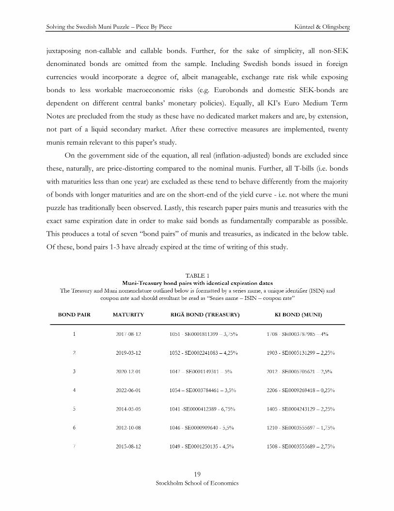
puzzle has traditionally been observed. Lastly, this research paper pairs munis and treasuries with the
exact same expiration date in order to make said bonds as fundamentally comparable as possible.
This produces a total of seven “bond pairs” of munis and treasuries, as indicated in the below table.
Of these, bond pairs 1-3 have already expired at the time of writing of this study.

Solving the Swedish Muni Puzzle – Piece By Piece Küntzel & Olingsberg
20
Stockholm School of Economics
Diagram 1: The ASW function illustrated by ownership and transaction branch. The value of the ASW, i.e. the ASW
price, is equivalent to the credit spread above or below LIBOR.
In studying the disparities between these seven paired Swedish muni and treasury returns, their daily
close-of-day prices are gathered from Bloomberg. Despite the paper’s efforts to control for some of
the varying characteristics demarcating KI and RiGä bonds, an attempt at bridging their different
coupons highlighted above is needed. In response to this, Bloomberg’s ASW (asset swap spread)
function is made use of. This command has seen repeated use in neighboring research including
Zaghinik (2014) and Pianiselli and Zaghini (2014), yet has to the best of our knowledge not directly
been used when examining the muni puzzle. In short, this input relates bond prices to an interest
rate swap in which Investor A longs the bond and enters into an interest rate swap with Financial
Institution B delivering the bond. Investor A pays a fixed rate and receives floating, effectively
transforming the fixed coupon on the bond into a (typically) LIBOR-based floating coupon. The
below diagram illustrates these ownership and transaction dynamics more carefully.
In this asset swap, the protection seller agrees to pay the protection buyer LIBOR +/- a
spread in return for the risky cash flows of the bond. In the event of default, the protection buyer
will continue to receive the LIBOR +/- a spread from the protection seller. This spread, then,
represents the credit spread between the bond’s risky coupon payments and the fixed-to-floating
swap rate. The value of the asset swap (i.e. the ASW price), therefore, must be this credit spread
over/under LIBOR. As with all derivatives, the intrinsic value of this asset swap is zero at inception,
yet with the passage of time and resulting changes in market conditions (ergo, dynamic LIBOR rates

Solving the Swedish Muni Puzzle – Piece By Piece Küntzel & Olingsberg
21
Stockholm School of Economics
and bond credit risks), the transaction hedge/asset swap derives a value and price. The ASW,
therefore, is nothing more than an interest rate hedge (fixed-to-floating) coupled with an insurance
policy against the bond cash flows’ credit risk, i.e. its probability of default. Naturally, both KI and
RiGä are privy to the same market-wide interest swap rate at any point in time. Equally, insurance
against their potential insolvencies ought to be equivalent given their identical statutory credit risks
and market-priced credit ratings. Accordingly, indistinguishable credit risks should translate to the
same credit spread, i.e. the same ASW price. The ASW function, therefore, effectively voids
differences in coupons while maintaining the risk characteristics inherent to the bonds.
Once done, comparable yields22 in the form of ASW prices are obtained for each of the
fourteen combined municipal and government bonds. When said bonds’ ASW yields then are
subtracted from one another, producing ASW yield differences, municipal ASW yields are reduced
by treasury ASW yields.
3.4 Empirical & Ethical Reflections
It is worth noting that all relevant cited academic literature herein is peer-reviewed and previously
cited. To the best of our knowledge, therefore, there is little to no reason to question the credibility
and legitimacy of the extant literature made use of in this study. Furthermore, all data collection
procedures have been limited to the use of Bloomberg, Thomson Reuters and information provided
from KommunInvest and are therefore, by and large, secondary information sources unencumbered
by the often greater care and concern implicit to the handling of primary sources. With respect to
the private discussions held with Mattias Bokenblom and Tobias Landström of KI, due
consideration was given in maintaining the integrity and representativeness of their voiced thoughts,
ideas and insights. Had this study investigated an area akin to the, for instance, aforementioned
Hamilton Project’s proposition of a communal body, a more socially sensitive nature would have
presented itself given the implications for taxpayers at stake.
22 Specifically, yields to maturities (YTM). Henceforth, all yield-related data is of the YTM sort and used interchangeably with the concepts of “yield” and “returns”.
Solving the Swedish Muni Puzzle – Piece By Piece Küntzel & Olingsberg
22
Stockholm School of Economics
IV. Analysis & Findings
In the following sections the paper presents the general properties of the ASW yield differences
between munis and treasuries, in turn mediating the effect liquidity has on these differences. In
minimizing the study’s exposure to statistical pitfalls, we examine the presence of heteroscedasticity
and autocorrelation before running a series of cross-sectional time-series FGLS (Feasible
Generalized Least Squares) panel regressions as well as a panel-correlated regression.
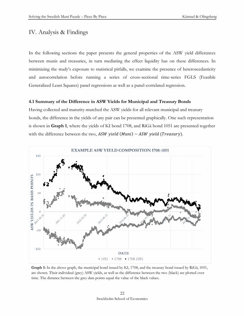
4.1 Summary of the Difference in ASW Yields for Municipal and Treasury Bonds
Having collected and maturity-matched the ASW yields for all relevant municipal and treasury
bonds, the difference in the yields of any pair can be presented graphically. One such representation
is shown in Graph 1, where the yields of KI bond 1708, and RiGä bond 1051 are presented together
with the difference between the two, 𝐴𝑆𝑊 𝑦𝑖𝑒𝑙𝑑 (𝑀𝑢𝑛𝑖) − 𝐴𝑆𝑊 𝑦𝑖𝑒𝑙𝑑 (𝑇𝑟𝑒𝑎𝑠𝑢𝑟𝑦).
Graph 1: In the above graph, the municipal bond issued by KI, 1708, and the treasury bond issued by RiGä, 1051,
are shown. Their individual (grey) ASW yields, as well as the difference between the two (black) are plotted over
time. The distance between the grey data points equal the value of the black values.
Solving the Swedish Muni Puzzle – Piece By Piece Küntzel & Olingsberg
23
Stockholm School of Economics
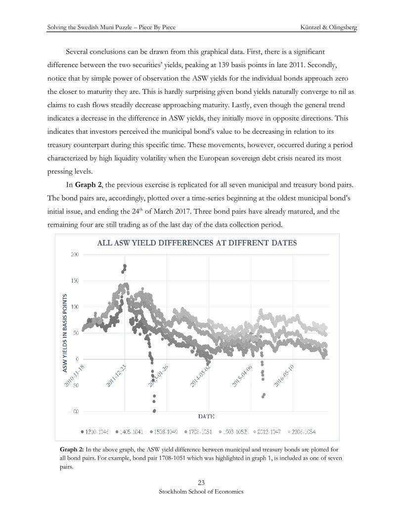
Graph 2: In the above graph, the ASW yield difference between municipal and treasury bonds are plotted for
all bond pairs. For example, bond pair 1708-1051 which was highlighted in graph 1, is included as one of seven
pairs.
Several conclusions can be drawn from this graphical data. First, there is a significant
difference between the two securities’ yields, peaking at 139 basis points in late 2011. Secondly,
notice that by simple power of observation the ASW yields for the individual bonds approach zero
the closer to maturity they are. This is hardly surprising given bond yields naturally converge to nil as
claims to cash flows steadily decrease approaching maturity. Lastly, even though the general trend
indicates a decrease in the difference in ASW yields, they initially move in opposite directions. This
indicates that investors perceived the municipal bond’s value to be decreasing in relation to its
treasury counterpart during this specific time. These movements, however, occurred during a period
characterized by high liquidity volatility when the European sovereign debt crisis neared its most
pressing levels.
In Graph 2, the previous exercise is replicated for all seven municipal and treasury bond pairs.
The bond pairs are, accordingly, plotted over a time-series beginning at the oldest municipal bond’s
initial issue, and ending the 24th of March 2017. Three bond pairs have already matured, and the
remaining four are still trading as of the last day of the data collection period.
Solving the Swedish Muni Puzzle – Piece By Piece Küntzel & Olingsberg
24
Stockholm School of Economics
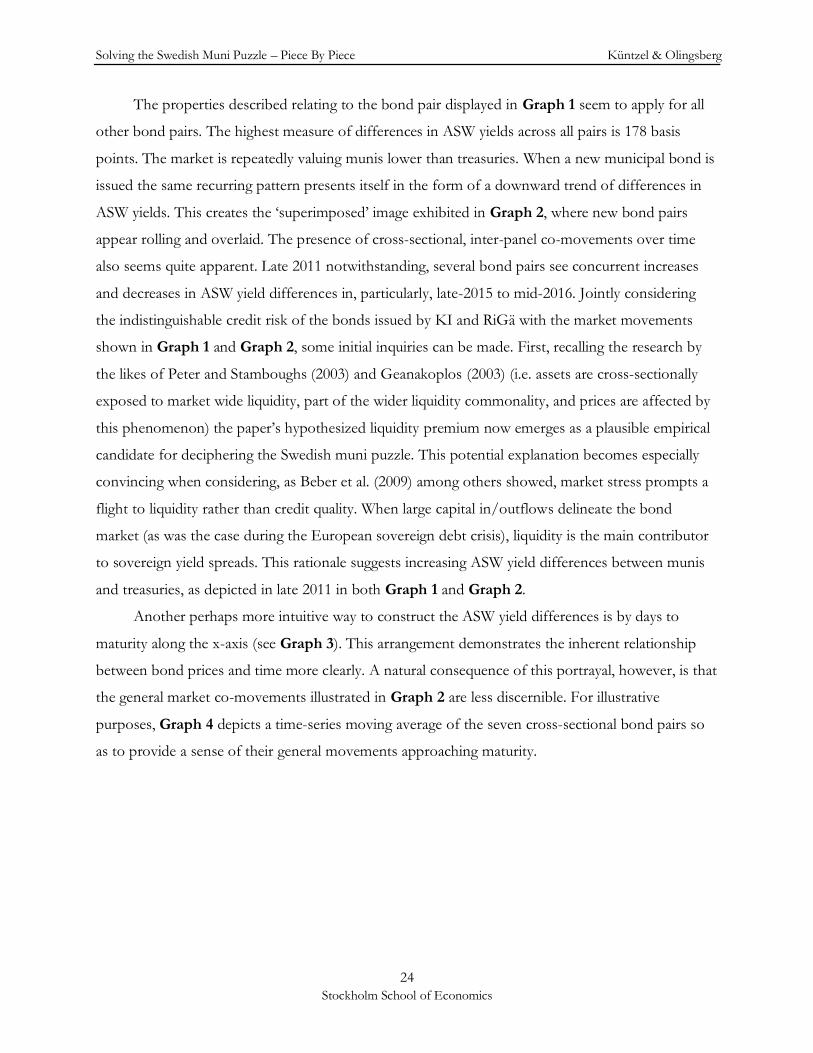
The properties described relating to the bond pair displayed in Graph 1 seem to apply for all
other bond pairs. The highest measure of differences in ASW yields across all pairs is 178 basis
points. The market is repeatedly valuing munis lower than treasuries. When a new municipal bond is
issued the same recurring pattern presents itself in the form of a downward trend of differences in
ASW yields. This creates the ‘superimposed’ image exhibited in Graph 2, where new bond pairs
appear rolling and overlaid. The presence of cross-sectional, inter-panel co-movements over time
also seems quite apparent. Late 2011 notwithstanding, several bond pairs see concurrent increases
and decreases in ASW yield differences in, particularly, late-2015 to mid-2016. Jointly considering
the indistinguishable credit risk of the bonds issued by KI and RiGä with the market movements
shown in Graph 1 and Graph 2, some initial inquiries can be made. First, recalling the research by
the likes of Peter and Stamboughs (2003) and Geanakoplos (2003) (i.e. assets are cross-sectionally
exposed to market wide liquidity, part of the wider liquidity commonality, and prices are affected by
this phenomenon) the paper’s hypothesized liquidity premium now emerges as a plausible empirical
candidate for deciphering the Swedish muni puzzle. This potential explanation becomes especially
convincing when considering, as Beber et al. (2009) among others showed, market stress prompts a
flight to liquidity rather than credit quality. When large capital in/outflows delineate the bond
market (as was the case during the European sovereign debt crisis), liquidity is the main contributor
to sovereign yield spreads. This rationale suggests increasing ASW yield differences between munis
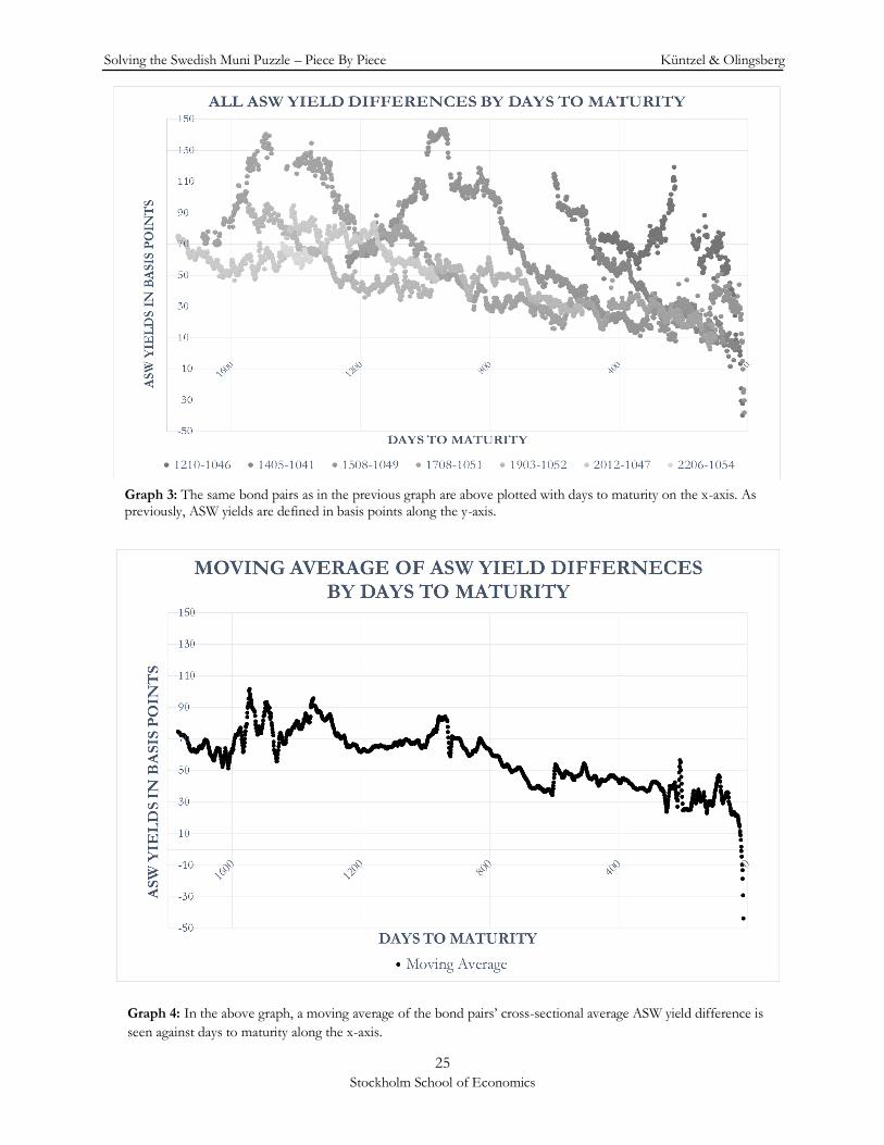
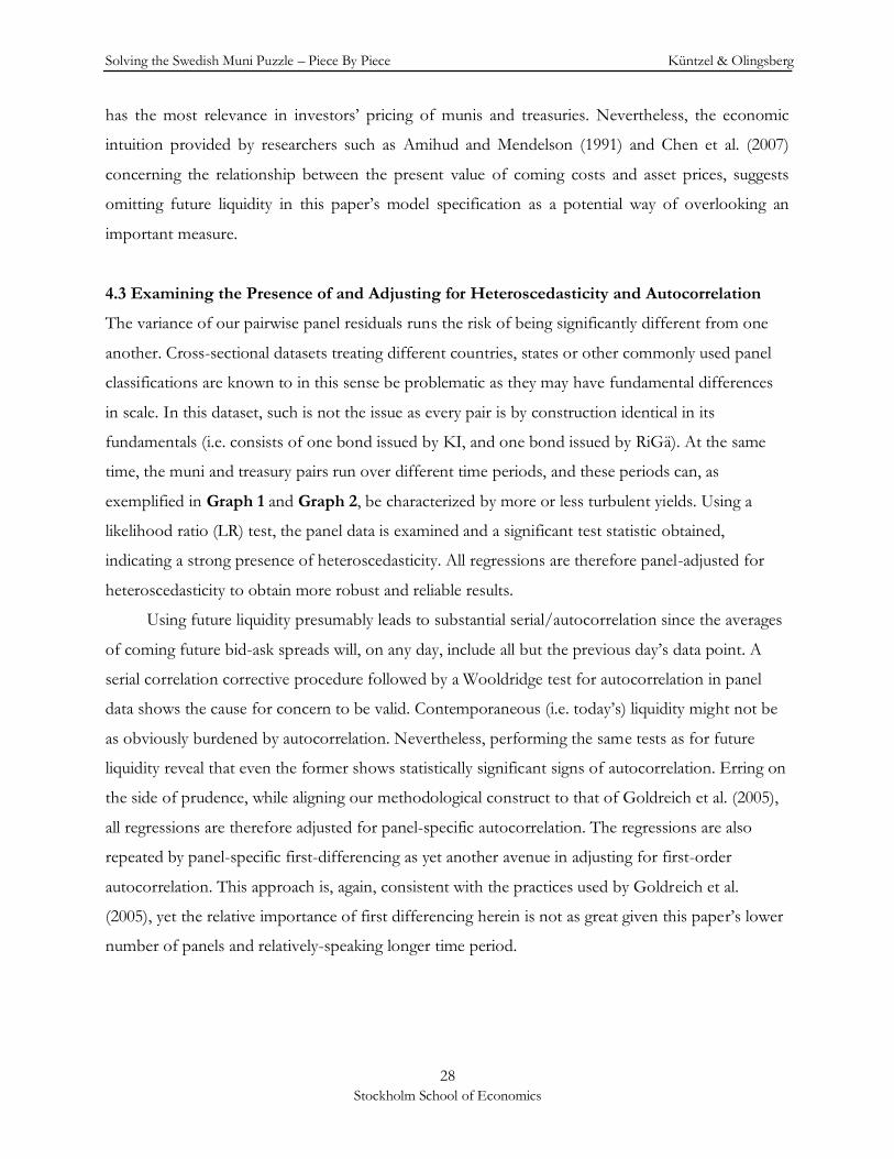
and treasuries, as depicted in late 2011 in both Graph 1 and Graph 2. Another perhaps more intuitive way to construct the ASW yield differences is by days to
maturity along the x-axis (see Graph 3). This arrangement demonstrates the inherent relationship
between bond prices and time more clearly. A natural consequence of this portrayal, however, is that
the general market co-movements illustrated in Graph 2 are less discernible. For illustrative
purposes, Graph 4 depicts a time-series moving average of the seven cross-sectional bond pairs so
as to provide a sense of their general movements approaching maturity.
Solving the Swedish Muni Puzzle – Piece By Piece Küntzel & Olingsberg
25
Stockholm School of Economics
Graph 4: In the above graph, a moving average of the bond pairs’ cross-sectional average ASW yield difference is
seen against days to maturity along the x-axis.
Graph 3: The same bond pairs as in the previous graph are above plotted with days to maturity on the x-axis. As previously, ASW yields are defined in basis points along the y-axis.

Solving the Swedish Muni Puzzle – Piece By Piece Küntzel & Olingsberg
26
Stockholm School of Economics
From this section we can conclude that in a setting without differences in default risk, taxes,
interest rate risk and underwriter reputation, there is still a substantial difference between the yields
of munis and treasuries to be accounted for. Though these aforementioned parameters are left un-
modeled in this paper and thus cannot be assigned any absolute or relative explanatory power,
Graph 1-4 support the notion that default risk and tax effects do not fully resolve the muni puzzle.
This study, instead, confines its resources to modelling liquidity premiums given its high contextual
relevance as a potential determinant of ASW yield differences. Ideally, this will contribute some
valuable insights as to how liquidity provides explanatory power to the muni puzzle, adding clarity to
the research field in the Swedish market and general bond market at large.
4.2 Describing the Variables and the Panel data
For every panel variable (i.e. bond pair), and every time interval in the relevant time series (i.e. date),
observations exist for both our dependent variable and independent variables. Our variables are
defined as follows.
Panel variable, P: 𝑃𝑎𝑖𝑟𝑛𝑢𝑚𝑏𝑒𝑟 = 1, 2, … , 7
Time Variable, t: 𝐷𝑎𝑡𝑒
Dependent variable:
For every 𝑃 𝑎𝑛𝑑 𝑡:
𝐴𝑆𝑊𝑀𝑇 = 𝐴𝑆𝑊 𝑦𝑖𝑒𝑙𝑑 (𝑀𝑢𝑛𝑖) − 𝐴𝑆𝑊 𝑦𝑖𝑒𝑙𝑑 (𝑇𝑟𝑒𝑎𝑠𝑢𝑟𝑦)
Independent variables:
For every 𝑃 𝑎𝑛𝑑 𝑡:, the contemporaneous (or current) cost of trading (i.e. liquidity premium,
expressed in basis points) for the individual bond can be defined as:
𝐶𝑜𝑛𝑡𝑒𝑚𝑝𝑜𝑟𝑎𝑛𝑒𝑜𝑢𝑠 𝐶𝑜𝑠𝑡 𝑜𝑓 𝑀𝑢𝑛𝑖: 𝐶𝑀 = 10000 ∙ 𝐴𝑠𝑘 − 𝐵𝑖𝑑
𝑀𝑖𝑑
𝐶𝑜𝑛𝑡𝑒𝑚𝑝𝑜𝑟𝑎𝑛𝑒𝑜𝑢𝑠 𝐶𝑜𝑠𝑡 𝑜𝑓 𝑇𝑟𝑒𝑎𝑠𝑢𝑟𝑦: 𝐶𝑇 = 10000 ∙ 𝐴𝑠𝑘 − 𝐵𝑖𝑑
𝑀𝑖𝑑
Solving the Swedish Muni Puzzle – Piece By Piece Küntzel & Olingsberg
27
Stockholm School of Economics
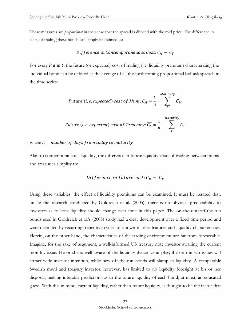
These measures are proportional in the sense that the spread is divided with the mid price. The difference in
costs of trading these bonds can simply be defined as:
𝐷𝑖𝑓𝑓𝑒𝑟𝑒𝑛𝑐𝑒 𝑖𝑛 𝐶𝑜𝑛𝑡𝑒𝑚𝑝𝑜𝑟𝑎𝑛𝑒𝑢𝑜𝑢𝑠 𝐶𝑜𝑠𝑡: 𝐶𝑀 − 𝐶𝑇
For every 𝑃 𝑎𝑛𝑑 𝑡, the future (or expected) cost of trading (i.e. liquidity premium) characterizing the
individual bond can be defined as the average of all the forthcoming proportional bid-ask spreads in
the time series:
𝐹𝑢𝑡𝑢𝑟𝑒 (𝑖. 𝑒. 𝑒𝑥𝑝𝑒𝑐𝑡𝑒𝑑) 𝑐𝑜𝑠𝑡 𝑜𝑓 𝑀𝑢𝑛𝑖: 𝐶𝑀 =
1
𝑛 ∙ ∑ 𝐶𝑀
𝑀𝑎𝑡𝑢𝑟𝑖𝑡𝑦
𝑡
𝐹𝑢𝑡𝑢𝑟𝑒 (𝑖. 𝑒. 𝑒𝑥𝑝𝑒𝑐𝑡𝑒𝑑) 𝑐𝑜𝑠𝑡 𝑜𝑓 𝑇𝑟𝑒𝑎𝑠𝑢𝑟𝑦: 𝐶𝑇 =
1
𝑛 ∙ ∑ 𝐶𝑇
𝑀𝑎𝑡𝑢𝑟𝑖𝑡𝑦
𝑡
Where 𝑛 = 𝑛𝑢𝑚𝑏𝑒𝑟 𝑜𝑓 𝑑𝑎𝑦𝑠 𝑓𝑟𝑜𝑚 𝑡𝑜𝑑𝑎𝑦 𝑡𝑜 𝑚𝑎𝑡𝑢𝑟𝑖𝑡𝑦
Akin to contemporaneous liquidity, the difference in future liquidity costs of trading between munis
and treasuries simplify to:
𝐷𝑖𝑓𝑓𝑒𝑟𝑒𝑛𝑐𝑒 𝑖𝑛 𝑓𝑢𝑡𝑢𝑟𝑒 𝑐𝑜𝑠𝑡: 𝐶𝑀 − 𝐶𝑇
Using these variables, the effect of liquidity premiums can be examined. It must be iterated that,
unlike the research conducted by Goldreich et al. (2005), there is no obvious predictability to
investors as to how liquidity should change over time in this paper. The on-the-run/off-the-run
bonds used in Goldreich et al.’s (2005) study had a clear development over a fixed time period and
were delimited by recurring, repetitive cycles of known market features and liquidity characteristics.
Herein, on the other hand, the characteristics of the trading environment are far from foreseeable.
Imagine, for the sake of argument, a well-informed US treasury note investor awaiting the current
monthly issue. He or she is well aware of the liquidity dynamics at play; the on-the-run issues will
attract wide investor intention, while new off-the-run bonds will slump in liquidity. A comparable
Swedish muni and treasury investor, however, has limited to no liquidity foresight at his or her
disposal, making inferable predictions as to the future liquidity of each bond, at most, an educated
guess. With this in mind, current liquidity, rather than future liquidity, is thought to be the factor that
Solving the Swedish Muni Puzzle – Piece By Piece Küntzel & Olingsberg
28
Stockholm School of Economics
has the most relevance in investors’ pricing of munis and treasuries. Nevertheless, the economic
intuition provided by researchers such as Amihud and Mendelson (1991) and Chen et al. (2007)
concerning the relationship between the present value of coming costs and asset prices, suggests
omitting future liquidity in this paper’s model specification as a potential way of overlooking an
important measure.
4.3 Examining the Presence of and Adjusting for Heteroscedasticity and Autocorrelation
The variance of our pairwise panel residuals runs the risk of being significantly different from one
another. Cross-sectional datasets treating different countries, states or other commonly used panel
classifications are known to in this sense be problematic as they may have fundamental differences
in scale. In this dataset, such is not the issue as every pair is by construction identical in its
fundamentals (i.e. consists of one bond issued by KI, and one bond issued by RiGä). At the same
time, the muni and treasury pairs run over different time periods, and these periods can, as
exemplified in Graph 1 and Graph 2, be characterized by more or less turbulent yields. Using a
likelihood ratio (LR) test, the panel data is examined and a significant test statistic obtained,
indicating a strong presence of heteroscedasticity. All regressions are therefore panel-adjusted for
heteroscedasticity to obtain more robust and reliable results. Using future liquidity presumably leads to substantial serial/autocorrelation since the averages
of coming future bid-ask spreads will, on any day, include all but the previous day’s data point. A
serial correlation corrective procedure followed by a Wooldridge test for autocorrelation in panel
data shows the cause for concern to be valid. Contemporaneous (i.e. today’s) liquidity might not be
as obviously burdened by autocorrelation. Nevertheless, performing the same tests as for future
liquidity reveal that even the former shows statistically significant signs of autocorrelation. Erring on
the side of prudence, while aligning our methodological construct to that of Goldreich et al. (2005),
all regressions are therefore adjusted for panel-specific autocorrelation. The regressions are also
repeated by panel-specific first-differencing as yet another avenue in adjusting for first-order
autocorrelation. This approach is, again, consistent with the practices used by Goldreich et al.
(2005), yet the relative importance of first differencing herein is not as great given this paper’s lower
number of panels and relatively-speaking longer time period.
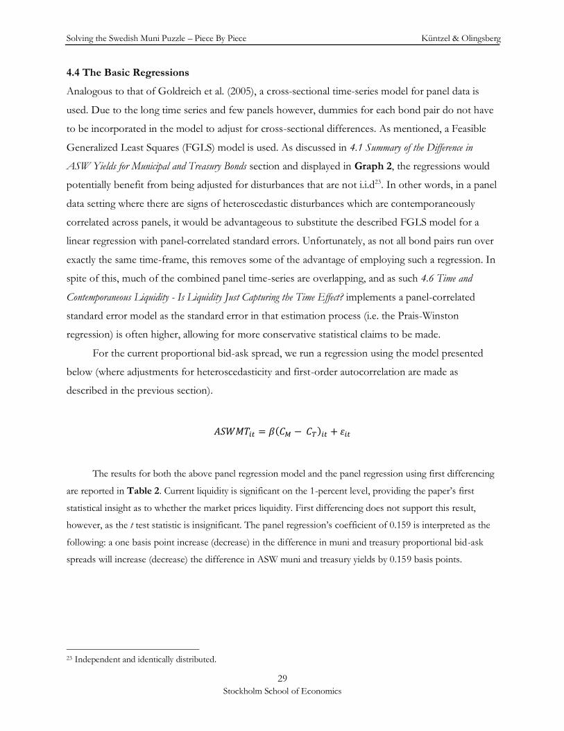
Solving the Swedish Muni Puzzle – Piece By Piece Küntzel & Olingsberg
29
Stockholm School of Economics
4.4 The Basic Regressions
Analogous to that of Goldreich et al. (2005), a cross-sectional time-series model for panel data is
used. Due to the long time series and few panels however, dummies for each bond pair do not have
to be incorporated in the model to adjust for cross-sectional differences. As mentioned, a Feasible
Generalized Least Squares (FGLS) model is used. As discussed in 4.1 Summary of the Difference in
ASW Yields for Municipal and Treasury Bonds section and displayed in Graph 2, the regressions would
potentially benefit from being adjusted for disturbances that are not i.i.d23. In other words, in a panel
data setting where there are signs of heteroscedastic disturbances which are contemporaneously
correlated across panels, it would be advantageous to substitute the described FGLS model for a
linear regression with panel-correlated standard errors. Unfortunately, as not all bond pairs run over
exactly the same time-frame, this removes some of the advantage of employing such a regression. In
spite of this, much of the combined panel time-series are overlapping, and as such 4.6 Time and
Contemporaneous Liquidity - Is Liquidity Just Capturing the Time Effect? implements a panel-correlated
standard error model as the standard error in that estimation process (i.e. the Prais-Winston
regression) is often higher, allowing for more conservative statistical claims to be made.
For the current proportional bid-ask spread, we run a regression using the model presented
below (where adjustments for heteroscedasticity and first-order autocorrelation are made as
described in the previous section).
𝐴𝑆𝑊𝑀𝑇𝑖𝑡 = 𝛽(𝐶𝑀 − 𝐶𝑇)𝑖𝑡 + 𝜀𝑖𝑡
The results for both the above panel regression model and the panel regression using first differencing
are reported in Table 2. Current liquidity is significant on the 1-percent level, providing the paper’s first
statistical insight as to whether the market prices liquidity. First differencing does not support this result,
however, as the t test statistic is insignificant. The panel regression’s coefficient of 0.159 is interpreted as the
following: a one basis point increase (decrease) in the difference in muni and treasury proportional bid-ask
spreads will increase (decrease) the difference in ASW muni and treasury yields by 0.159 basis points.
23 Independent and identically distributed.
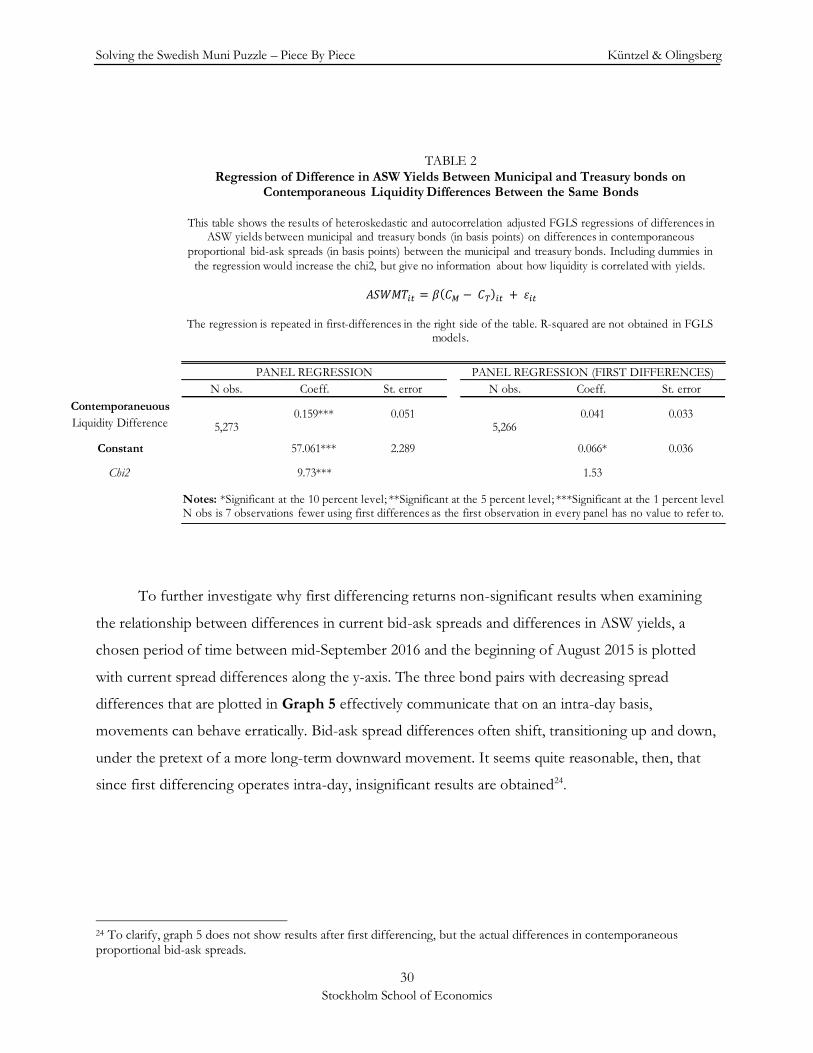
Solving the Swedish Muni Puzzle – Piece By Piece Küntzel & Olingsberg
30
Stockholm School of Economics
To further investigate why first differencing returns non-significant results when examining
the relationship between differences in current bid-ask spreads and differences in ASW yields, a
chosen period of time between mid-September 2016 and the beginning of August 2015 is plotted
with current spread differences along the y-axis. The three bond pairs with decreasing spread
differences that are plotted in Graph 5 effectively communicate that on an intra-day basis,
movements can behave erratically. Bid-ask spread differences often shift, transitioning up and down,
under the pretext of a more long-term downward movement. It seems quite reasonable, then, that
since first differencing operates intra-day, insignificant results are obtained24.
24 To clarify, graph 5 does not show results after first differencing, but the actual differences in contemporaneous proportional bid-ask spreads.
N obs. Coeff. St. error N obs. Coeff. St. error
Constant 57.061*** 2.289 0.066* 0.036
Chi2
Contemporaneuous
Liquidity Difference0.159*** 0.051 0.041
9.73*** 1.53
PANEL REGRESSION PANEL REGRESSION (FIRST DIFFERENCES)
0.0335,273 5,266
Notes: *Significant at the 10 percent level; **Significant at the 5 percent level; ***Significant at the 1 percent level. N obs is 7 observations fewer using first differences as the first observation in every panel has no value to refer to.
TABLE 2
Regression of Difference in ASW Yields Between Municipal and Treasury bonds on Contemporaneous Liquidity Differences Between the Same Bonds
This table shows the results of heteroskedastic and autocorrelation adjusted FGLS regressions of differences in ASW yields between municipal and treasury bonds (in basis points) on differences in contemporaneous
proportional bid-ask spreads (in basis points) between the municipal and treasury bonds. Including dummies in
the regression would increase the chi2, but give no information about how liquidity is correlated with yields.
𝐴𝑆𝑊𝑀𝑇𝑖𝑡 = 𝛽 𝐶𝑀 − 𝐶𝑇 𝑖𝑡 + 𝜀𝑖𝑡
The regression is repeated in first-differences in the right side of the table. R-squared are not obtained in FGLS models.
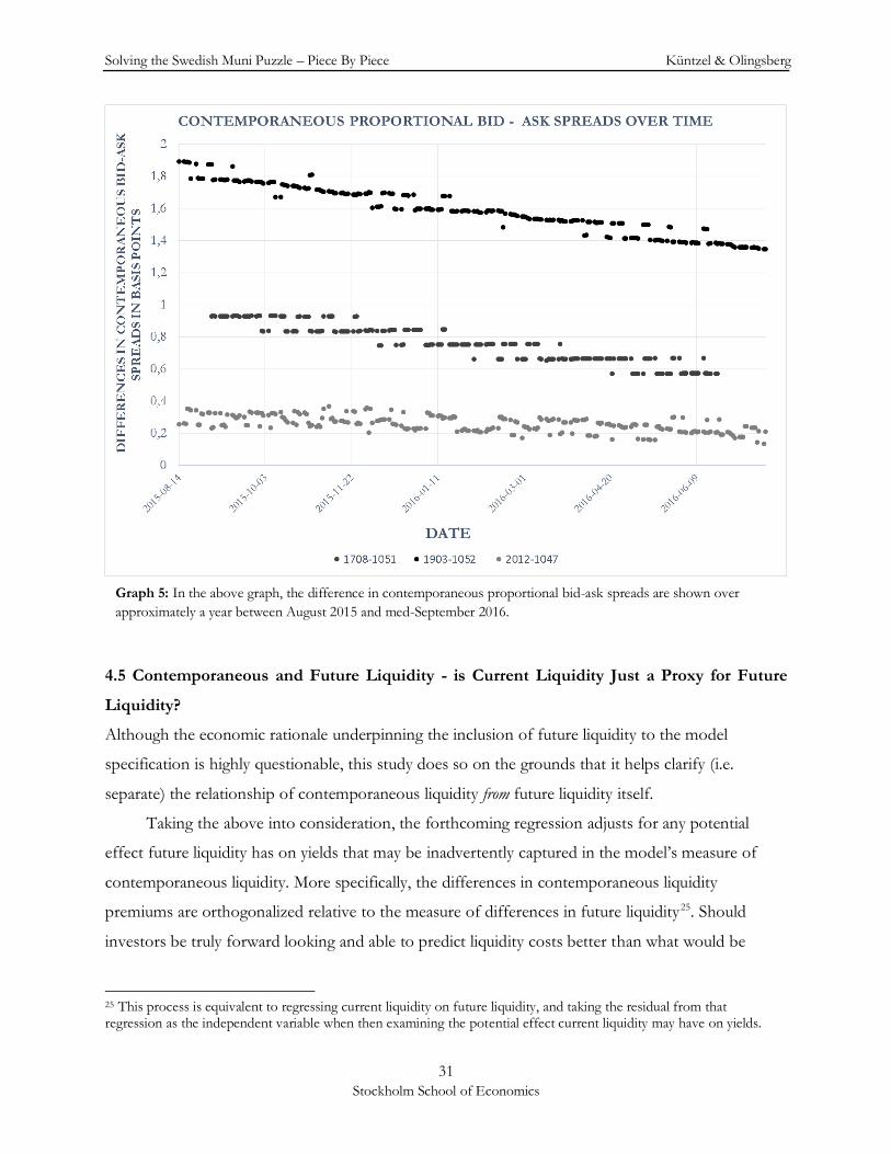
Solving the Swedish Muni Puzzle – Piece By Piece Küntzel & Olingsberg
31
Stockholm School of Economics
4.5 Contemporaneous and Future Liquidity - is Current Liquidity Just a Proxy for Future
Liquidity?
Although the economic rationale underpinning the inclusion of future liquidity to the model
specification is highly questionable, this study does so on the grounds that it helps clarify (i.e.
separate) the relationship of contemporaneous liquidity from future liquidity itself.
Taking the above into consideration, the forthcoming regression adjusts for any potential
effect future liquidity has on yields that may be inadvertently captured in the model’s measure of
contemporaneous liquidity. More specifically, the differences in contemporaneous liquidity
premiums are orthogonalized relative to the measure of differences in future liquidity25. Should
investors be truly forward looking and able to predict liquidity costs better than what would be
25 This process is equivalent to regressing current liquidity on future liquidity, and taking the residual from that regression as the independent variable when then examining the potential effect current liquidity may have on yields.
Graph 5: In the above graph, the difference in contemporaneous proportional bid-ask spreads are shown over
approximately a year between August 2015 and med-September 2016.

Solving the Swedish Muni Puzzle – Piece By Piece Küntzel & Olingsberg
32
Stockholm School of Economics
expected given the lack of foreseeable cycles of liquidity, one would anticipate the orthogonalized
measure of current liquidity to be stripped of most of its explanatory power. With that said, the now
modified equation used to examine ASW yields follows:
𝐴𝑆𝑊𝑀𝑇𝑖𝑡 = 𝛶(𝐶𝑀 − 𝐶𝑇)𝑖𝑡𝑜𝑟𝑡ℎ + 𝛽(𝐶𝑀
− 𝐶𝑇 )𝑖𝑡 + 𝜀𝑖𝑡
Table 3 shows the results obtained from the above regression as well as the panel regression
using first-differencing. Having now considered future liquidity, the test statistic in the panel
regression indicates differences in contemporaneous liquidity between munis and treasuries can help
explain our dependent variable, ASWMT. Differences in future liquidity are also significant in this
regression, which challenges this study’s voiced a priori expectations given the innate difficulty
investors experience in gauging future muni and treasury liquidity. Reinterpreting this result,
however, the reader should bear in mind that the orthogonalized nature of contemporaneous
liquidity leaves its shared explanatory power with future liquidity in future liquidity itself. Using an
orthogonalized measure in the regression is by construction a way of allowing a separate, more easily
understood coefficient of contemporaneous liquidity. Even though future liquidity is
N obs. Coeff. St. error N obs. Coeff. St. error
Constant 58.079*** 2.318 0.065* 0.036
Chi2
14.02*** 2.59
PANEL REGRESSION PANEL REGRESSION (FIRST DIFFERENCES)
2.0292.3720.6181.340**
0.261Orthogonalized
Contemporaneuous
Liquidity Difference
1.277*** 0.423 0.287
Future Liquidity
Difference
5,273 5,266
Notes: *Significant at the 10 percent level; **Significant at the 5 percent level; ***Significant at the 1 percent level. N obs is 7 observations fewer using first differences as the first observation in every panel has no value to refer to.
TABLE 3Regression of Difference in ASW Yields Between Municipal and Treasury bonds on Orthogonalized
Contemporaneous liquidity Differences and Future Liquidity Differences Between the Same Bonds
This table shows the results of heteroskedastic and autocorrelation adjusted FGLS regressions of differences in ASW yields between municipal and treasury bonds (in basis points) on differences in orthogonalized
contemporaneous and future (averaged) proportional bid-ask spreads (in basis points) between the municipal and treasury bonds. The coefficient on the orthogonalized contemporaneous liquidity difference is stripped of any
explanatory power relative future liquidity differences.
𝐴𝑆𝑊𝑀𝑇𝑖𝑡 = 𝛶(𝐶𝑀 − 𝐶𝑇)𝑖𝑡𝑜𝑟𝑡ℎ + 𝛽 𝐶𝑀 − 𝐶𝑇 𝑖𝑡 + 𝜀𝑖𝑡
The regression is repeated in first-differences in the right side of the table.
Solving the Swedish Muni Puzzle – Piece By Piece Küntzel & Olingsberg
33
Stockholm School of Economics
statistically significant at the 5-percent level, differences in future liquidity in the form of average
proportional bid-ask spreads cannot confidently be concluded to have causal implications on the
prices of bonds. Moreover, as previously mentioned, there is little to lackluster economic intuition
for subsuming investors can accurately predict muni and treasury liquidity changes. With respect to
the first-differencing panel regression, the results are not significant for either liquidity measure,
echoing the findings of Goldreich et al. (2005) after looking at intra-day changes over their time-
series. In brief, including future liquidity and orthogonalizing contemporaneous (current) liquidity
has served as an exercise to better separate the two, after which future liquidity is promptly excluded
for the same economic reasons as alluded to previously.
4.6 Time and Contemporaneous Liquidity - Is Liquidity Just Capturing the Time Effect?
Due to the inherent relationship between time and yields, a variable comprised of days to maturity is
added to the model specification, in line with Goldreich et al.’s (2005) design. If the measure of
differences in contemporaneous liquidity is just capturing time to maturity, the obtained results
would be spurious and have no ‘real’ explanatory power. The model is therefore re-specified in the
following way:
𝐴𝑆𝑊𝑀𝑇𝑖𝑡 = 𝛽𝜏𝑖𝑡 + 𝛶(𝐶𝑀 − 𝐶𝑇)𝑖𝑡𝑜𝑟𝑡ℎ + 𝜀𝑖𝑡
Notice that the measure of differences in future liquidity between the bond types is no longer
included in the model, as motivated in the previous section. A question that may have occurred to
the reader, at this point, asks why the panel is not set with days to maturity (as opposed to date) as
the relevant cross-sectional time-series input. It might indeed, at first glance, seem appropriate given
the natural relationship displayed in Graph 3. Statistical methods intent on doing so, however,
would unfortunately make it impossible to apply the aforementioned linear regression with panel-
correlated standard errors, discussed in greater depth shortly.
The results from the above specified regression are reported in Table 4. No first-differencing
is reported this time as the collinearity in the resulting differenced days to maturity variable would be
exceedingly high - an output value of -1 would consistently be obtained, set aside those few dates
dropped due to missing ASW yields. The current liquidity bid-ask spread differences are still highly
significant, despite a slightly lower coefficient, when taking into consideration days left to maturity.
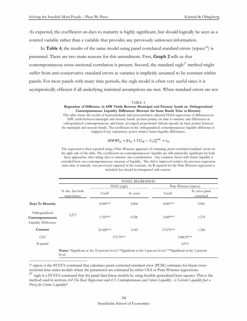
Solving the Swedish Muni Puzzle – Piece By Piece Küntzel & Olingsberg
34
Stockholm School of Economics
As expected, the coefficient on days to maturity is highly significant, but should logically be seen as a
control variable rather than a variable that provides any previously unknown information.
In Table 4, the results of the same model using panel correlated standard errors (xtpsce26) is
presented. There are two main reasons for this amendment. First, Graph 2 tells us that
contemporaneous cross-sectional correlation is present. Second, the standard xtgls27 method might
suffer from anti-conservative standard errors as variance is implicitly assumed to be constant within
panels. For most panels with many time periods, the xtgls model is often very useful since it is
asymptotically efficient if all underlying statistical assumptions are met. When standard errors are not
26 xtpcse is the STATA command that calculates panel-corrected standard error (PCSE) estimates for linear cross-sectional time-series models where the parameters are estimated by either OLS or Prais-Winsten regressions. 27 xtgls is a STATA command that fits panel-data linear models by using feasible generalized least squares. This is the method used in sections 4.4 The Basic Regressions and 4.5. Contemporaneous and Future Liquidity - is Current Liquidity Just a Proxy for Future Liquidity?
N obs. (for both
regressions)Coeff. St. error Coeff.
St. error panel
correlated
Constant 21.020*** 3.149 17.675*** 1.336
Chi2
R-sqaured
Orthogonalized
Contemporaneuous
Liquidity Difference
0.044*** 0.004 0.041*** 0.001Days To Maturity
PANEL REGRESSION
FGLS (xtgls) Prais-Winston (xtpcse)
173.79*** 1348.55***
1.155*** 0.326 3.669*** 1.274
0.073
5,273
Notes: *Significant at the 10 percent level; **Significant at the 5 percent level; ***Significant at the 1 percent level.
TABLE 4Regression of Difference in ASW Yields Between Municipal and Treasury bonds on Orthogonalized
Contemporaneous Liquidity Differences Between the Same Bonds Time to Maturity
This table shows the results of heteroskedastic and autocorrelation adjusted FGLS regressions of differences in ASW yields between municipal and treasury bonds (in basis points) on time to maturity and differences in
orthogonalized contemporaneous and future (averaged) proportional bid-ask spreads (in basis points) between
the municipal and treasury bonds. The coefficient on the orthogonalized contemporaneous liquidity difference is stripped of any explanatory power relative future liquidity differences.
𝐴𝑆𝑊𝑀𝑇𝑖𝑡 = 𝛽𝜏𝑖𝑡 + 𝛶(𝐶𝑀 − 𝐶𝑇)𝑖𝑡𝑜𝑟𝑡ℎ + 𝜀𝑖𝑡
The regression is then repeated using a Prais-Winston approach of estimating penel correlated standard errors on
the right side of the table. The coefficients on contemporaneuous liquidity are still statistically significant for both these approaches after taking days to maturity into consideration. Any common factor with future liquidity is
excluded from our contemporaneuous measure of liquidity. The chi2 is improved relative the previous regression since time to maturity was previously captured in the constant. An R-squared for the Prais-Winston regression is
included, but should be interpreted with caution.
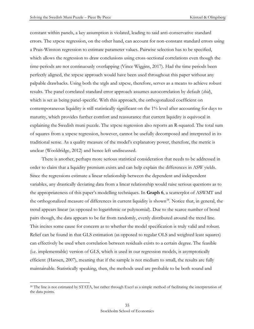
Solving the Swedish Muni Puzzle – Piece By Piece Küntzel & Olingsberg
35
Stockholm School of Economics
constant within panels, a key assumption is violated, leading to said anti-conservative standard
errors. The xtpcse regression, on the other hand, can account for non-constant standard errors using
a Prais-Winston regression to estimate parameter values. Pairwise selection has to be specified,
which allows the regression to draw conclusions using cross-sectional correlations even though the
time-periods are not continuously overlapping (Vince Wiggins, 2017). Had the time periods been
perfectly aligned, the xtpcse approach would have been used throughout this paper without any
palpable drawbacks. Using both the xtgls and xtpcse, therefore, serves as a means to achieve robust
results. The panel correlated standard error approach assumes autocorrelation by default (ibid),
which is set as being panel-specific. With this approach, the orthogonalized coefficient on
contemporaneous liquidity is still statistically significant on the 1% level after accounting for days to
maturity, which provides further comfort and reassurance that current liquidity is equivocal in
explaining the Swedish muni puzzle. The xtpcse regression also reports an R-squared. The total sum
of squares from a xtpcse regression, however, cannot be usefully decomposed and interpreted in its
traditional sense. As a quality measure of the model’s explanatory power, therefore, the metric is
unclear (Wooldridge, 2012) and hence left undiscussed.
There is another, perhaps more serious statistical consideration that needs to be addressed in
order to claim that a liquidity premium exists and can help explain the differences in ASW yields.
Since the regressions estimate a linear relationship between the dependent and independent
variables, any drastically deviating data from a linear relationship would raise serious questions as to
the appropriateness of this paper’s modelling techniques. In Graph 6, a scatterplot of ASWMT and
the orthogonalized measure of differences in current liquidity is shown28. Notice that, in general, the
trend appears linear (as opposed to logarithmic or polynomial). Due to the scarce number of bond
pairs though, the data appears to be far from randomly, evenly distributed around the trend line.
This incites some cause for concern as to whether the model specification is truly valid and robust.
Relief can be found in that GLS estimation (as opposed to regular OLS and weighted least squares)
can effectively be used when correlation between residuals exists to a certain degree. The feasible
(i.e. implementable) version of GLS, which is used in our regression models, is asymptotically
efficient (Hansen, 2007), meaning that if the sample is not medium to small, the results are fully
maintainable. Statistically speaking, then, the methods used are probable to be both sound and
28 The line is not estimated by STATA, but rather through Excel as a simple method of facilitating the interpretation of the data points.
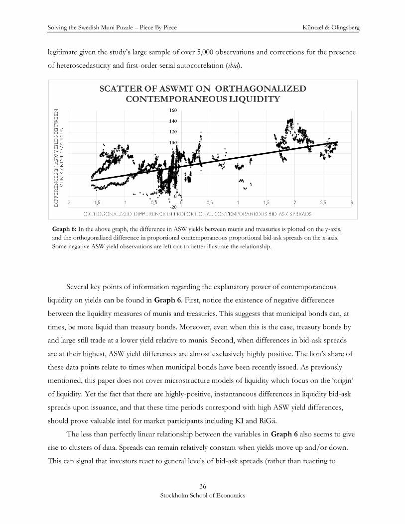
Solving the Swedish Muni Puzzle – Piece By Piece Küntzel & Olingsberg
36
Stockholm School of Economics
legitimate given the study’s large sample of over 5,000 observations and corrections for the presence
of heteroscedasticity and first-order serial autocorrelation (ibid).
Several key points of information regarding the explanatory power of contemporaneous
liquidity on yields can be found in Graph 6. First, notice the existence of negative differences
between the liquidity measures of munis and treasuries. This suggests that municipal bonds can, at
times, be more liquid than treasury bonds. Moreover, even when this is the case, treasury bonds by
and large still trade at a lower yield relative to munis. Second, when differences in bid-ask spreads
are at their highest, ASW yield differences are almost exclusively highly positive. The lion’s share of
these data points relate to times when municipal bonds have been recently issued. As previously
mentioned, this paper does not cover microstructure models of liquidity which focus on the ‘origin’
of liquidity. Yet the fact that there are highly-positive, instantaneous differences in liquidity bid-ask
spreads upon issuance, and that these time periods correspond with high ASW yield differences,
should prove valuable intel for market participants including KI and RiGä. The less than perfectly linear relationship between the variables in Graph 6 also seems to give
rise to clusters of data. Spreads can remain relatively constant when yields move up and/or down.
This can signal that investors react to general levels of bid-ask spreads (rather than reacting to
Graph 6: In the above graph, the difference in ASW yields between munis and treasuries is plotted on the y-axis,
and the orthogonalized difference in proportional contemporaneous proportional bid-ask spreads on the x-axis.
Some negative ASW yield observations are left out to better illustrate the relationship.

Solving the Swedish Muni Puzzle – Piece By Piece Küntzel & Olingsberg
37
Stockholm School of Economics
changes in liquidity on an intra-day basis) and trade on that information. Such an interpretation
would not contradict previous research or compromise the consensus understanding of flight-to-
liquidity which, during times of market distress, need not be precipitated on drastic changes to
liquidity in the short-term. Examining the region around the general trend-line’s y-intercept in Graph 6 (i.e. the model’s
constant), the ASW yields are largely contained to the 10 to 100 basis points span. In the same vein,
the regressions that take days to maturity into consideration (which is difficult to illustrate in two-
dimensional space) estimate their model constants’ 95% confidence interval to be 14.84 to 27.12 and
15.06 to 20.29 for the xtgls and xtpcse regression respectively. Both model variants scrutinized,
therefore, showcase a sizeable and significant difference in ASW yields left to be explained even
after accounting for liquidity.
4.7 Relating the Results to the Muni Puzzle
Having amended differences in current proportional bid-ask spreads through orthogonalization
while accounting for days left to maturity in modelling differences in ASW yields, we are left with
the task of relating the paper’s findings to the muni puzzle. Given the hard-to-decipher R-squared of
the regression based upon an FGLS approach, the interpretation of the results are grounded in other
rationales. Specifically, a general discussion of the statistical power of our explanatory variables put
in relation to the setting of this study is relevant. To recapitulate, the reader should recognize that in
this study’s climate, there should not be any default risk, tax-risk difference or varying exposure to
the yield curve (i.e. interest rate risk) at work in the differences in ASW yields. Having limited the
scope of this study to modelling liquidity, the only variables potentially omitted are those completely
overlooked or neglected in 2.2 Literature Survey. One such determinant springs to mind: the elusive
and fleeting investor attention. Whether omitted or unnoticed, these variables undoubtedly seem to
matter, as conveyed by the large (~20 basis points) and statistically significant model constants
presented. These constants open up for interesting discussions regarding asset pricing factors that
may not have been generally discussed in research examining the muni puzzle. At the same time, the
panel regressions in sections 4.4-4.6 reveal a rather compelling story: contemporaneous liquidity
matters in explaining yield differences between municipal and government bonds over the maturity
spectrum, thus helping to explain the Swedish muni puzzle.
Solving the Swedish Muni Puzzle – Piece By Piece Küntzel & Olingsberg
38
Stockholm School of Economics
4.8 Concluding remarks
Differences in ASW yields reached levels of 178 basis points during the European sovereign debt
crisis. Clearly, there are important asset pricing factors that differ between the two bond types:
munis and treasuries. Liquidity premiums are a well-suited candidate in explaining the muni puzzle
residual in an institutional context unencumbered by tax, credit or interest rate risk differentials in
the municipal and government space. Operationalized as the commonly used measure of
(proportional, contemporaneous) bid-ask spreads, liquidity premiums are statistically significant
using two types of Feasible Generalized Least Squares (FGLS) methods. Discontinuous patterns of
rather stagnant differences in current proportional bid-ask spreads under a longer downward trend
suggest investors might not be reacting to short-term changes in liquidity. This observed
phenomenon also makes first differencing less reliable and telling. Moreover, a highly significant
constant shows absent variables remain important, opening up for discussions as to what
unconsidered determinants in this paper’s literature survey could potentially be influential in
explaining the muni puzzle.
V. Discussion & Critical Reflections
Having analyzed a substantial amount of market movements and statistics, the results will now be
critically reflected upon, related to the research question and put in context using the elements
discussed in the theoretical framework. Three ways the results in this paper can be incorporated in
other research are also discussed. Finally, the paper’s findings are discussed from the view of societal
knowledge contribution and implications for policymakers.
5.1 Connecting the Findings to Theory
Akin to Longstaff et al. (2005) and Bao et al. (2011), this paper demonstrates that the component of
the yield not due to credit risk is time varying. Longstaff et al. (2005) also presented evidence that
this residual component is related to macro liquidity measures in the bond market. No liquidity
measures for the market (or models incorporating sensitivity to market wide liquidity) are presented
in this paper, but given the known bond market characteristics during the European debt crisis,
there are clear indications that the bonds analyzed in this paper also move with market wide
liquidity.

Solving the Swedish Muni Puzzle – Piece By Piece Küntzel & Olingsberg
39
Stockholm School of Economics
Having delineated and analyzed the way bid-ask spreads behave both over time and relative to
yields in the municipal and treasury bond market, it is more easily understood as to why a large
corpus of measures continue to proxy liquidity in past and current research. Contemporaneous
proportional bid-ask spreads, which should capture liquidity in an effective manner relative to many
other measures, still experience the setbacks and odd movements displayed and described in Graph
5 and Graph 6. Bao et al. (2011) and Amihud and Mendelson (1991) argue that liquidity is properly
modeled if changes in measures of costs give rise to changes in bond prices. A natural consequence
of the data characteristics in this study is then, of course, that this criterion cannot be met on a day-
to-day basis due to the persistence in bid-ask spreads visible in Graph 5.
Some discrepancies are, however, to be expected between previous theory and the findings of
new studies. It is especially reasonable to expect results which do not conform to earlier research
when a method and logic (adapted from Goldreich et al. (2005)) is applied on an unfamiliar problem
(i.e. the muni puzzle) in a market where the conundrum in question has not historically been
addressed (i.e. the Swedish bond market).
Findings from Peng and Lin (2007) and Da and Zhi (2011) who analyzed the implications of
investor attention on financial markets have been briefly mentioned, but otherwise generally
overlooked. Whether the effect of an inclusion of variables capturing differences in investor
attention would have been great enough to account for the documented constant in the model is a
question future research ought to dedicate time and effort to.
5.2 The Research Question in a Broader Sense
The aim of this paper is not to solve the concept of the muni puzzle in its broadest sense. Indeed,
such an undertaking would be to misunderstand the limitations of this study. In the US, which is
where the muni puzzle is primarily discussed, researchers must consider default risk and tax
implications together with liquidity, and consequently assign relative importance to these factors. A
similar strategy is clearly not relevant in Sweden. Instead, the results can complement the research
conducted in a more multi-factor market setting. There are at least three ways this paper can be
considered in other research. Researchers can: (i) compare the unexplained difference between
municipal and treasury bonds after their adjustment for credit risk and see if it resembles the data
presented in section 4.1 Summary of the Difference in ASW Yields for Municipal and Treasury Bonds29 , (ii)
29 Of course, other aspects must be considered simultaneously so as not to wrongly assume the Swedish municipal and treasury bonds are equivalent to the market instruments under study.
Solving the Swedish Muni Puzzle – Piece By Piece Küntzel & Olingsberg
40
Stockholm School of Economics
use the sections 4.4 Basic Regressions to 4.7 Relating the Results to the Muni Puzzle to potentially clear up
some confusion whether liquidity matters after already having considered the aspects which are
naturally eliminated in the Swedish market, (iii) further examine whether any remaining asset pricing
factors have a significant enough explanatory power to ‘fill the gap’ that the constant in the final
model in section 4.7 Relating the Results to the Muni Puzzle now occupies.
5.3 Knowledge Contribution and Implications for Policymakers
KI can be studied by initiative takers including the academics, business leaders and former public
policy makers behind the Hamilton project (discussed in I. introduction). Since KI has successfully
lowered the borrowing costs for the Swedish municipalities, it can serve as an example not just for
the US, but also other countries internationally. The results discussed in section 4.7 Relating the Results
to the Muni Puzzle have further implications for policymakers where organizational bodies pooling
municipal bonds are already implemented. The fact that there is still a yield differential between KI’s
and RiGä’s bonds having considered liquidity implies that policymakers might have to consider
other aspects like investor attention. Implementing an organizational body similar to KI might not,
therefore, be enough to lower the costs associated with providing financing to municipalities to
desired levels.
5.4 Future Research Given the significant constant in the regression models, further research is needed to fully
understand the Swedish muni puzzle and with it, the muni puzzle at large. Identifying and
quantifying other factors than credit risk, tax related effects, interest rate risk, and underwriter
reputation could also be of interest internationally.
Future research could also examine the effect of quantitative easing (QE) on the yields of
municipal and treasury bonds. In Sweden, QE is an extensively used monetary policy. Interestingly,
KI has in an open letter to the Swedish central bank asked them not to buy their bonds for liquidity
reasons (Munkhammar, 2016).
Solving the Swedish Muni Puzzle – Piece By Piece Küntzel & Olingsberg
41
Stockholm School of Economics
VI. Limitations of research 6.1 Data Accessing data for all bond pairs needed to calculate relevant, valid measures of liquidity proved to
be difficult. Consequently, the conclusions relating to whether a liquidity premium can explain the
Swedish muni puzzle are exclusively based on measures of the bid-ask spread. Including other
measures could potentially strengthen or nuance the view of the existence of a liquidity premium.
Then again, the proportional bid-ask spread has proven to be a highly valid measure of liquidity in
the related literature, and its significance using two statistical methods in this paper reinforces that
finding. Furthermore, including certain variables for reasons only pertaining to the quantity of
coefficients can have undesired effects. For example, consider the study by Aitken and Carole (2003)
where the researchers study volume before and after the crisis on the Jakarta Exchange. The results
indicated a sharp, 51% trading volume increase, suggesting the crisis had positive implications on
liquidity. The market consensus, on the other hand, was that a liquidity crisis was unfolding.
Using finer data, such as hourly or minute data, would from a purely theoretical standpoint be
closer to the essence of liquidity, and could potentially capture the relationship between yields and
liquidity in a different fashion. Then again, the reader should recall that finer data is not necessarily
more accurate, and the value added to the analysis of such an inclusion might not be worth the time
and effort that it entails. Adding more data points in a paper like this might be particularly useless
when considering the already discontinuous patterns characterizing bid-ask spreads (apparent in
Graph 5).
Analyzing a larger amount of bond pairs would, however, be beneficial to the study. Seven
bond pairs are quite substantially fewer than the 55 that are used in the research by Goldreich et al.
(2005). Relatively few panels, with different lengths, running over different periods, become
statistically challenging. Furthermore, graphical presentations and interpretations become more
difficult, burdening the economic intuition, with data displaying these characteristics. The scarcity of
bond pairs comes with a silver lining, however: having excluded real bonds, T-bills, callable bonds
and non-SEK denominated bonds, as well as only used bonds with perfectly matched maturity
dates, the data set becomes highly statistically analyzable without extensive model-modifications.
Consequently, the results of this paper do not have to rely on yield curve extrapolation or any other
type of estimation procedure which relies on assumptions about risks, investor behavior or other
asset pricing factors. The same cannot be said about the method of Goldreich et al. (2005), for
Solving the Swedish Muni Puzzle – Piece By Piece Küntzel & Olingsberg
42
Stockholm School of Economics
instance, where corrections for asynchronous quotes are made to avoid the distortionary effects
intraday interest rate changes may have on obtained results. Moreover, to fairly compare papers
regarding the data sample, one should consider the lengths of the time series. For some bond pairs,
the series ranges several years, whereas in Goldreich et al. (2005), and of course other similar
research, the series are considerably shorter. In total, this paper considers over 5,200 observations,
compared to the 1,210 in the paper from Goldreich et al. (2005)30.
6.2 Models One primary limitation regarding the model used is that the regressions and estimated coefficients
are difficult to interpret. The dependent variable is expressed in basis points (in a yield difference
context). The independent variable is also expressed in basis points, but in an orthogonalized form
and based on a difference in two proportions (as defined in 4.2. Describing the Variables and Our Panel
Data). This might cause confusion, especially given that the panel correlated method yields a
coefficient which differs from the standard cross-sectional time-series FGLS regression. If future,
(i.e. average) liquidity had been of primary interest, the coefficient on that variable could have been
interpreted as the marginal investor’s per-year probability of trading31. In a conservative manner, the
reader of this paper should instead consider the statistically significant coefficient as a general
indication for the correlation between trading liquidity differences and yield differences.
Another limitation in this paper is that the clientele effect due to investment horizons has not
been modeled. A nonlinear relationship can in theory exists between liquidity and yields. There are
two reasons for why this phenomenon has not been examined further. First, drawing inspiration
from Goldreich et al. (2005), who does not make such a correction, the risks from including clientele
effects (e.g. risks of model misspecification or further complicating the coefficient interpretation)
was believed to be higher than the potential benefits associated with its implementation. Secondly,
no clear indication for a nonlinear-relationship was found.
One aspect that has been consistently discussed throughout this paper is how investor
attention is thought to affect yields. The lack of modeling of such a factor undoubtedly affects this
paper’s capability in drawing more nuanced conclusions. One can further imagine that liquidity and
investor attention are (positively) correlated, introducing omitted variable bias in the regression
30 Of course, the papers are not perfectly comparable since Goldreich et al. (2005) averages their dependent variable by the cross section of bond pairs, and also uses seven measures of liquidity in total. 31 The reader is directed to Goldreich et al. (2005) and Amihud and Mendelson (1985) for the intuition behind this interpretation.
Solving the Swedish Muni Puzzle – Piece By Piece Küntzel & Olingsberg
43
Stockholm School of Economics
models. As discussed in 2.2.5 Investor Attention though, collecting and analyzing relevant information
is not always easy. Even with google search frequency based measures, such a procedure is not
straightforward. Discussions regarding market efficiencies would realistically also have to be
incorporated, which complicates the analysis drastically.
VII. Conclusion
With comparable credit risk and identical tax treatment, the municipal and treasury bonds issued by
KommunInvest (the Swedish Local Government Debt Office) and Riksgälden (the Swedish National
Debt Office) respectively, serve as ideal candidates for examining the impact of liquidity premiums
on bond yields. Using data from Bloomberg and Thomson Reuters, this paper finds that despite the
fundamental similarities between Swedish munis and treasuries, a substantial and enduring difference
in their (ASW) yields exists in the longer end of the yield curve, reaching levels of 178 basis points
during the European sovereign debt crisis. This is the Swedish embodiment of the more traditionally
US-dominated muni puzzle. In examining the research question “Can liquidity premiums explain the
Swedish Muni Puzzle?", non-callable, SEK-denominated, non-real munis are paired with perfectly
maturity-matched treasuries - yielding a total of seven bond pairs stretching over a combined 5,200
observations between September, 2010 and March, 2017.
Liquidity differences are operationalized as the proportional bid-ask spread of the muni
subtracted by the proportional bid-ask spread of its treasury pair. To estimate a measure of future
liquidity, all coming contemporaneous (current) measures of liquidity are averaged at each time t.
Orthogonalizing differences in contemporaneous liquidity relative the differences in future liquidity,
the effect of current liquidity is isolated. Adjusting for days to maturity, the ASW yields of the seven
bond pairs are regressed against the orthogonalized measure of differences in contemporaneous
liquidity bid-ask spreads. In the final model, both a cross-sectional time-series Feasible Generalized
Least Squares (FGLS) method adjusted for heteroscedasticity and panel-specific autocorrelation and
a panel correlated standard error regression are used.
The coefficients on the measure of liquidity are statistically significant on a 1 percent level for
both regressions, thus suggesting liquidity premiums help explain the Swedish muni puzzle. A
constant in the region of ~20 basis points also opens up for discussions regarding thus far
potentially overlooked variables, including investor attention. Three ways our research can be

Solving the Swedish Muni Puzzle – Piece By Piece Küntzel & Olingsberg
44
Stockholm School of Economics
incorporated and considered in other, future research are suggested. Policymakers having
implemented similar organizations to KommunInvest would be wise not to neglect due
consideration for the muni puzzle’s antecedents other than its mainstream determinants, captured in
this paper’s constant.

Solving the Swedish Muni Puzzle – Piece By Piece Küntzel & Olingsberg
45
Stockholm School of Economics
Reference List
Acharya, V.V. & Pedersen, L.H. 2005, "Asset pricing with liquidity risk", Journal of Financial Economics, vol. 77, no. 2, pp. 375-410.
Aitken, M. & Winn, R. 1997, "What is this thing called liquidity", Securities Industry Research Center of Asia Pacific Sydney, Australia, .
Aitken, M. & Comerton-Forde, C. 2003, "How should liquidity be measured?", Pacific-Basin Finance Journal, vol. 11, no. 1, pp. 45-59.
Amihud, Y. & Mendelson, H. 1991, "Liquidity, asset prices and financial policy", Financial Analysts Journal, , pp. 56-66.
Amihud, Y. & Mendelson, H. 1986, "Asset pricing and the bid-ask spread", Journal of Financial Economics, vol. 17, no. 2, pp. 223-249.
Amihud, Y., Mendelson, H. & Pedersen, L.H. 2006, "Liquidity and asset prices", Foundations and Trends® in Finance, vol. 1, no. 4, pp. 269-364.
Ang, A. & Green, R. 2011, Lowering Borrowing Costs for States and Municipalities Through CommonMuni, The Hamilton Project, Washington.
Ang, J., Peterson, D. & Peterson, P. 1985, "Marginal Tax Rates: Evidence from Nontaxable Corporate Bonds: A Note", The Journal of Finance, vol. 40, no. 1, pp. 327-332.
Baltagi, B.H. 2011, Econometrics, 5th edn, Springer.
BAO, J., PAN, J. & WANG, J. 2011, "The Illiquidity of Corporate Bonds", The Journal of Finance, vol. 66, no. 3, pp. 911-946.
Beber, A., Brandt, M.W. & Kavajecz, K.A. 2009, "Flight-to-quality or flight-to-liquidity? Evidence from the euro-area bond market", Review of Financial Studies, vol. 22, no. 3, pp. 925-957.
Boudoukh, J. & Whitelaw, R.F. 1993, "Liquidity as a choice variable: A lesson from the Japanese government bond market", Review of Financial Studies, vol. 6, no. 2, pp. 265-292.
Bryman, A. 2012, Social Research Methods, 4th edn, Oxford University Press, Oxford.
Campbell, T.S. 1980, "On the Extent of Segmentation in the Municipal Securities Market", Journal of Money, Credit and Banking, vol. 12, no. 1, pp. 71-83.
Chalmers, J.M.R. 2006, "Systematic Risk and the Muni Puzzle", National Tax Journal, vol. 59, no. 4, pp. 833-848.
Solving the Swedish Muni Puzzle – Piece By Piece Küntzel & Olingsberg
46
Stockholm School of Economics
CHAN, K.C., KAROLYI, G.A., LONGSTAFF, F.A. & SANDERS, A.B. 1992, "An Empirical Comparison of Alternative Models of the Short-Term Interest Rate", The Journal of Finance, vol. 47, no. 3, pp. 1209-1227.
Chen, L., Lesmond, D.A. & Wei, J. 2007, "Corporate Yield Spreads and Bond Liquidity", The Journal of Finance, vol. 62, no. 1, pp. 119-149.
Choudhry, M. 2010, "Measuring bond market liquidity: devising a composite aggregate liquidity score", Applied Financial Economics, vol. 20, no. 12, pp. 955-973.
Codogno, L., Favero, C. & Missale, A. 2003, "Yield spreads on EMU government bonds", Economic Policy, vol. 18, no. 37, pp. 503-532.
Constantinides, G.M. & Ingersoll, J.E. 1982, "Optimal Bond Trading with Personal Tax: Implications for Bond Prices and Estimated Tax Brackets and Yield Curves", The Journal of Finance, vol. 37, no. 2, pp. 349-352.
Cook, T.Q. & Hendershott, P.H. 1978, "The Impact of Taxes, Risk and Relative Security Supplies on Interest Rate Differentials", The Journal of Finance, vol. 33, no. 4, pp. 1173-1186.
DA, Z., ENGELBERG, J. & GAO, P. 2011, "In Search of Attention", The Journal of Finance, vol. 66, no. 5, pp. 1461-1499.
Daniels, K.N. & Vijayakumar, J. 2007, "Does underwriter reputation matter in the municipal bond market?", Journal of economics and business, vol. 59, no. 6, pp. 500-519.
Duffee, G.R. 2002, "Term Premia and Interest Rate Forecasts in Affine Models", The Journal of Finance, vol. 57, no. 1, pp. 405-443.
ERICSSON, J. & RENAULT, O. 2006, "Liquidity and Credit Risk", The Journal of Finance, vol. 61, no. 5, pp. 2219-2250.
FANG, L.H. 2005, "Investment Bank Reputation and the Price and Quality of Underwriting Services", The Journal of Finance, vol. 60, no. 6, pp. 2729-2761.
Fisher, L. 1959, "Determinants of risk premiums on corporate bonds", Journal of Political Economy, vol. 67, no. 3, pp. 217-237.
Fontaine, J. & Garcia, R. 2012, "Bond Liquidity Premia", The Review of Financial Studies, vol. 25, no. 4, pp. 1207-1254.
FORTUNE, P. 1973, "THE IMPACT OF TAXABLE MUNICIPAL BONDS: POLICY SIMULATIONS WITH A LARGE ECONOMETRIC MODEL", National Tax Journal, vol. 26, no. 1, pp. 29-42.
Geanakoplos, J. 2001, "Liquidity, default and crashes: Endogenous contracts in general equilibrium", .
Solving the Swedish Muni Puzzle – Piece By Piece Küntzel & Olingsberg
47
Stockholm School of Economics
Gilchrist, S., Yankov, V. & Zakrajšek, E. 2009, "Credit market shocks and economic fluctuations: Evidence from corporate bond and stock markets", Journal of Monetary Economics, vol. 56, no. 4, pp. 471-493.
Goldreich, D., Hanke, B. & Nath, P. 2005, "The Price of Future Liquidity: Time-Varying Liquidity in the U. S. Treasury Market", Review of Finance, vol. 9, no. 1, pp. 1-32.
Göta Hovrätt 1994, Kommun har inte ansetts kunna försättas i konkurs, Swedish Court of Appeal.
Goyenko, R.Y., Holden, C.W. & Trzcinka, C.A. 2009, "Do liquidity measures measure liquidity?", Journal of Financial Economics, vol. 92, no. 2, pp. 153-181.
Graham, J.R. & Rogers, D.A. 2002, "Do Firms Hedge in Response to Tax Incentives?", The Journal of Finance, vol. 57, no. 2, pp. 815-839.
Hansen, C.B. 2007, "Generalized least squares inference in panel and multilevel models with serial correlation and fixed effects", Journal of Econometrics, vol. 140, no. 2, pp. 670-694.
Hasbrouck, J. & Seppi, D.J. 2001, "Common factors in prices, order flows, and liquidity", Journal of Financial Economics, vol. 59, no. 3, pp. 383-411.
Hastie, K.L. 1972, "Determinants of Municipal Bond Yields", The Journal of Financial and Quantitative Analysis, vol. 7, no. 3, pp. 1729-1748.
Hong, G. & Warga, A. 2000, "An empirical study of bond market transactions", Financial Analysts Journal, , pp. 32-46.
Houweling, P., Mentink, A. & Vorst, T. 2005, "Comparing possible proxies of corporate bond liquidity", Journal of Banking & Finance, vol. 29, no. 6, pp. 1331-1358.
Huberman, G. & Halka, D. 2001, "Systematic liquidity", Journal of Financial Research, vol. 24, no. 2, pp. 161-178.
John, M.R.C. 1998, "Default Risk Cannot Explain the Muni Puzzle: Evidence from Municipal Bonds That are Secured by U.S. Treasury Obligations", The Review of Financial Studies, vol. 11, no. 2, pp. 281-308.
Kidwell, D.S. & Koch, T.W. 1983, "Market Segmentation and the Term Structure of Municipal Yields", Journal of Money, Credit and Banking, vol. 15, no. 1, pp. 40-55.
King, G., Keohane, R.O. & Verba, S. 1995, "The importance of research design in political science", American Political Science Review, vol. 89, no. 02, pp. 475-481.
Klompenhouwer, A.J., Verver, D., Janki, S., Bramer, W.M., Doukas, M., Dwarkasing, R.S., de Man, R.A. & IJzermans, J.N. 2017, "Management of hepatic angiomyolipoma: A systematic review", Liver international : official journal of the International Association for the Study of the Liver, .

Solving the Swedish Muni Puzzle – Piece By Piece Küntzel & Olingsberg
48
Stockholm School of Economics
Kommuninvest 2017, , Annual Report 2016, Kommuninvest i Sverige AB. Available: http://kommuninvest.se/wp-content/uploads/2017/02/KIAB_2016_ENG.pdf [2017, March 26].
Kommuninvest 2016, , Swedish Local Government Debt Office. Available: http://kommuninvest.se/wp-content/uploads/2017/01/Kommuninvest-2016-12-21_ENG.pdf [2017, March 26].
KommunInvest 2017, How we became the largest lender to the Swedish local government sector. Available: http://kommuninvest.se/en/about-us-3/our-history/ [2017, March 25].
KORTEWEG, A. 2010, "The Net Benefits to Leverage", The Journal of Finance, vol. 65, no. 6, pp. 2137-2170.
Li, H., Wang, J., Wu, C. & He, Y. 2009, "Are Liquidity and Information Risks Priced in the Treasury Bond Market?", The Journal of Finance, vol. 64, no. 1, pp. 467-503.
Lin, H., Wang, J. & Wu, C. 2011, "Liquidity risk and expected corporate bond returns", Journal of Financial Economics, vol. 99, no. 3, pp. 628-650.
Liu, S., Wang, J. & Wu, C. 2003, "Effects of Credit Quality on Tax-Exempt and Taxable Yields", The Journal of Fixed Income, vol. 13, no. 2, pp. 80-99.
Longstaff, F.A. 2011, "Municipal debt and marginal tax rates: Is there a tax premium in asset prices?", The Journal of Finance, vol. 66, no. 3, pp. 721-751.
LONGSTAFF, F.A., MITHAL, S. & NEIS, E. 2005, "Corporate Yield Spreads: Default Risk or Liquidity? New Evidence from the Credit Default Swap Market", The Journal of Finance, vol. 60, no. 5, pp. 2213-2253.
Mackenzie, K.D. & House, R. 1978, "Paradigm development in the social sciences: A proposed research strategy", Academy of Management Review, vol. 3, no. 1, pp. 7-23.
Miller, M.H. 1977, "Debt and Taxes", The Journal of Finance, vol. 32, no. 2, pp. 261-275.
Modigliani, F. & Miller, M.H. 1958, "The Cost of Capital, Corporation Finance and the Theory of Investment", The American Economic Review, vol. 48, no. 3, pp. 261-297.
Munkhammar, V. 2016, , Kommuninvest: Köp inte våra obligationer. Available: http://www.di.se/nyheter/kommuninvest-kop-inte-vara-obligationer/ [2017, 05/14].
Norden, L. & Weber, M. 2009, "The Co-movement of Credit Default Swap, Bond and Stock Markets: an Empirical Analysis", European Financial Management, vol. 15, no. 3, pp. 529-562.
Pashler, H., Johnston, J.C. & Ruthruff, E. 2001, "Attention and performance", Annual Review of Psychology, vol. 52, no. 1, pp. 629-651.
Pasquariello, P. & Vega, C. 2009, "The on-the-run liquidity phenomenon", Journal of Financial Economics, vol. 92, no. 1, pp. 1-24.
Solving the Swedish Muni Puzzle – Piece By Piece Küntzel & Olingsberg
49
Stockholm School of Economics
Pástor, Ľ. & Stambaugh, R.F. 2003, "Liquidity risk and expected stock returns", Journal of Political economy, vol. 111, no. 3, pp. 642-685.
Peng, L. & Xiong, W. 2006, "Investor attention, overconfidence and category learning", Journal of Financial Economics, vol. 80, no. 3, pp. 563-602.
Peng, L., Xiong, W. & Bollerslev, T. 2007, "Investor Attention and Time-varying Comovements", European Financial Management, vol. 13, no. 3, pp. 394-422.
Pianeselli, D. & Zaghini, A. 2014, "The cost of firms’ debt financing and the global financial crisis", Finance Research Letters, vol. 11, no. 2, pp. 74-83.
Regeringskansliet 2004, Lag (2004:773) om kommunalekonomisk utjämning.
Regeringskansliet 1991, Kommunallag (1991:900).
Riksgälden 2014, , Rating. Available: https://www.riksgalden.se/en/For-investerare/policy-regelverk/Rating/ [2017, March 26].
Salmon, W.C. 1989, "Four decades of scientific explanation", Scientific explanation, vol. 13, pp. 3-219.
Sarig, O. & Warga, A. 1989, "Bond Price Data and Bond Market Liquidity", The Journal of Financial and Quantitative Analysis, vol. 24, no. 3, pp. 367-378.
Trzcinka, C. 1982, "The Pricing of Tax-Exempt Bonds and the Miller Hypothesis", The Journal of Finance, vol. 37, no. 4, pp. 907-923.
Vayanos, D. 1998, "Transaction costs and asset prices: A dynamic equilibrium model", Review of Financial Studies, vol. 11, no. 1, pp. 1-58.
Vince Wiggins, S. , How does xtgls differ from regression clustered with robust standard errors? Comparing xtgls with regress, vce(cluster). Available: http://www.stata.com/support/faqs/statistics/xtgls-versus-regress/ [2017, 05-12].
Wooldridge, J.M. 2012, Introductory Econometrics: A Modern Approach, p. 426, 5th edn, South-Western College Pub.
Yawitz, J.B., Maloney, K.J. & Ederington, L.H. 1985, "Taxes, Default Risk, and Yield Spreads", The Journal of Finance, vol. 40, no. 4, pp. 1127-1140.
Zaghini, A. 2014, "Bank bonds: size, systemic relevance and the sovereign", International Finance, vol. 17, no. 2, pp. 161-184.