Embed Size (px)
Citation preview

Solving the Prize-collecting Rural Postman Problem
Julian AraozSimon Bolıvar University∗, Venezuela
Technical University of Catalonia†, Spain
Elena FernandezTechnical University of Catalonia, Spain
Oscar Meza‡
Simon Bolıvar University, Venezuela.
Abstract
In this work we present an algorithm for solving the Prize-collecting Rural PostmanProblem. This problem was recently defined and is a generalization of other arc routingproblems like, for instance, the Rural Postman Problem. The main difference is that thereare no required edges. Instead, there is a profit function on the edges that must be takeninto account only the first time that an edge is traversed.
The problem is modeled as a linear integer program where the system has an exponentialnumber of inequalities. We propose a solution algorithm where iteratively we solve relaxedmodels with a small number of inequalities, that provide upper bounds, and we proposeexact separation procedures for generating violated cuts when possible. We also propose asimple heuristic to generate feasible solutions that provide lower bounds at each iteration.We use a two-phase method with different solvers at each phase.
Despite the difficulty of the problem, the numerical results from a series of computationalexperiments with various types of instances assess the good behavior of the algorithm. Inparticular, 75% of the instances were optimally solved with the LP relaxation of the model.The remaining instances were optimally solved on a second phase, most of them in smallcomputation times.
∗Retired Professor Dpt. Process and Systems.†Visiting Professor Dpt. Statistics and Operation Research.‡Retired Professor Dpt. Computation and Information Technology
1

1 Introduction
In this work we present an algorithm to solve the Prize-collecting Rural Postman Problem(PRPP). This problem was defined in Araoz, Fernandez and Zoltan [5] with the name Priva-tized Rural Postman Problem, and is part of the family of Arc Routing Problems (ARPs), thatusually aim to determine a least-cost traversal of a specified arc subset of a graph, with orwithout constraints. Such problems arise in a variety of practical contexts, like post deliveryand garbage collection. Typical constraints of ARPs require the routes to begin and to finish ata given point (the depot), and guarantee the connectivity of the solutions with the depot. Werefer the reader to Dror [17] for a comprehensive state on the art of such problems. Here weconsider only Edge Routing Problems (ERPs), which are the undirected cases of ARPs.
Like in other ERPs, in the PRPP we assume that the demand of service is placed at theedges of a graph. However, there is no specific arc subset to be traversed. Instead, we assumethat giving service to an edge not only would incur a cost (associated with displacement), butwould also result on a profit (associated with servicing edges). The displacement cost to anedge will certainly account for the cost of all the edges that are traversed in the same route,as many times as they are traversed. Similarly, the profit associated with servicing an edge,must also take into account the profit of the additional edges that are serviced in the sameroute. However, the profit of each edge serviced in the route will be collected only once, inde-pendently of the number of times the edge is traversed. In the PRPP we look for traversals thatmaximize the total servicing profit minus the displacement cost. As shown in [5] the Rural Post-man Problem (RPP) is a particular case of PRPP. In fact, PRPPs constitute a generalization ofmost ERPs with one single route and is equivalent to most Traveling Salesman Problems (TSPs).
The motivation for studying the PRPP comes not only from its theoretical interest but alsofrom its potential applications. In general, the applications of classical ERPs defined as mini-mization problems arise in public administrations and assume that it has been decided a priorithat the service to be given is essential at certain demand sites. Thus, the goal is not to decidethe edges to attend, but which is a least cost traversal. However, in the context of privatecompanies looking to maximize operational profits, a demand edge would not be serviced unlessit would result on a benefit for the company. As an example we can mention the collection ofrecycling bins by a private entity. Additionally, problems of this type might appear as subprob-lems in the pricing stage when addressing capacitated ERPs by column generation.
To the best of our knowledge, the literature on ERPs with profits on the edges is scarce.Apart from [5] and our previous works [3, 2], we are aware of only two works, one by Deitch andLadany [16] and another one by Feillet, Dejax and Gendreau [19] where problems of this typeare considered. In both papers the setting and the approach are quite different from ours: whileour approach addresses the problem as an arc-routing one and exploits the fact that only thefirst traversal of edges is beneficial, in [16] the problem is transformed into a node-routing one,and in [19] a limit, possibly greater than one, is given on the number of times the visit is benefi-cial on an edge. We are not aware of any work where a solution method is proposed for the PRPP.
2

In this work we model the PRPP by means of a linear system with an exponential number ofinequalities, based on the one defined in [5], and we propose an algorithm to solve the problem.The algorithm is composed of two phases. Each phase consists of an iterative process, where ateach iteration the following steps are performed:
i) Solving a relaxation of PRPP;
ii) Applying a simple heuristic (an adaptation of the 3T heuristic of Fernandez, Meza, Garfinkeland Ortega [18] for the Rural Postman Problem) to find a feasible solution;
iii) Solving the separation problem for finding different types of inequalities violated by theoptimal solution to the current relaxation; and,
iv) Adding the violated inequalities to the current system.
Thus, at the end of each iteration we have an upper bound to the original problem (given bythe solution to the relaxed problem), and a lower bound (given by the value of the feasiblesolution obtained with the heuristic). Since the original system has an exponential number ofinequalities, at both phases we consider relaxations of PRPP where only a small subset of theinequalities are included. The difference between the two phases is the type of relaxation thatis considered: Linear Programming (LP) problems at the first phase, and integer problems (IP)at the second phase. Both phases terminate either when optimality can be proven or when nomore violated cuts can be generated. A flowchart with a general scheme of the algorithm isdepicted in Figure 1.
FIGURE 1 HERE
Figure 1: Flowchart of the solution algorithm.
Despite the difficulty of the problem, the numerical results from a series of computational ex-periments with various types of instances assess the good behavior of the algorithm, since inmost cases the problems are solved in small computation times.
The paper is structured as follows. In Section 2 we define the problem and recall from [5]some properties of its solutions. The formulation that we use is presented in Section 3. Section 4describes the steps of the iterative process, including the initial relaxation of the problem. Theexact separation algorithms, both for the inequalities that guarantee the parity of the nodesand for the inequalities that guarantee connectivity of the solutions with the depot are given inSection 5. Section 6 describes the heuristic that has been used to obtain feasible solutions and,thus, lower bounds. In Section 7 we describe the computational experiments and present theobtained results. We finish the paper in Section 8 with the conclusions and some remarks.
3
2 The Prize-collecting Rural Postman Problem
2.1 Notation and Nomenclature
As usual G = (V,E) is a undirected graph with vertex set V , |V | = n, and edge set E, |E| = m.For any subgraph H we denote by V (H) the vertex set of H and by E(H) the edge set of H, inparticular, V = V (G), E = E(G). Let S be a non-empty proper subset of V , we denote by:
δ(S) = {e ∈ E|e = (u, v), u ∈ S, v ∈ V \ S} = δ(V \ S), the edges in the cut between S andV \ S, and
γ(S) = {e ∈ E|e = (u, v), u, v ∈ S}, the edges with both vertices in S.
Therefore given ∅ ⊂ S ⊂ V , E is partitioned in three sets γ(S), δ(S) = δ(V \ S), and γ(V \ S).For a singleton set we do not use the brackets and we write δ(v) ≡ δ({v}).
For any edge set F ⊆ E, the set of vertices incident to edges in F is denoted V (F ). Thesubgraph induced by F is G(F ) = (V (F ), F ). For any vertex set U ⊆ V we denote G[U ] theinduced graph (U, γ(U)).
We use the standard compact notation f(A) ≡∑
e∈A fe when A ⊆ E, and f is a vector ora function defined on E. If f is defined on a subset B ⊂ E we also use f(A) ≡ f(A ∩ B) ≡∑
e∈A∩B fe. Also, by extension, if H is a graph we denote f(H) ≡ f(E(H)).
We next recall from [5] the definitions and results relevant for our algorithm.
Definition 2.1 Prize-collecting Rural Postman Problem (PRPP).
Given a graph G(V,E) with a distinguished vertex d, the Depot, and two functions from Ein IR+, the profit function b and the cost function c, the Prize-collecting Rural Postman Problemis to find one closed path C∗ which maximizes the value of∑
e∈C(be − tece)
where C is a closed path in G passing trough d, and not necessarily simple, and te is the numberof times that edge e is traversed in C.
We denote a PRPP by (G, d, b, c).
That is, in a PRPP, we look for the most Profitable Subtour passing through d. Like in otherarc routing problems defined on undirected graphs, in PRPP we allow for consecutive traversalsof the same edge in both directions, and trees traversed two times define feasible solutions. In[5] it was proven that, in general, the PRPP is NP–Hard. In [5] it was also proven that whenthe underlying graph is a tree, then the PRPP can be solved in polynomial time.
4

We define the functions ϕe = be − ce and ψe = be − 2ce = ϕe − ce. Since, the value ϕe is thenet profit obtained the first time that edge e is traversed, and −ce is the net profit in each ofthe subsequent traversals of edge e, ψe is the the net profit of edge e when it is traversed twice.In the PRPP the edges in R = {e ∈ E | ψe ≥ 0} play an important role, similar to the set ofrequired edges in a RPP.
We denote by GR ≡ (V (R)∪{d}, R) the subgraph induced by the edge set R and the depot.Let Ck, k ∈ P = {0, . . . , p} be the connected components of the graph GR and we assume thatd ∈ C0. Using standard graph nomenclature, when necessary, we denote by Vk = V (Ck), andwe differentiate between γ(Vk) in the original graph G and γR(Vk) in the graph GR. That isγR(Vk) = γ(Vk) ∩R. Similarly, for S ⊂ V , δR(S) = δ(S) ∩R.
Let C∗ denote an optimal solution. The following properties hold:
2.2 Dominance 1. No edge is used more than twice in C∗.
2.3 Dominance 2. If an edge e ∈ E is used with value ce in C∗, then it is also used with valueϕe in C∗.
2.4 Dominance 3. Let e ∈ C∗, if for some connected component Ck of GR we have thatV (e) ∩ Vk 6= ∅ then all the edges of γR(Vk) are in C∗.
Remark 2.5 Dominance 3 implies that either all the edges of γR(Vk) are in C∗, or none of themis in C∗. Throughout, for each k ∈ P , eRk is chosen to be one of the edges in Ck with greatestϕe.
Note that Dominance 3 also implies that if any edge not in R incident with a vertex in Vk isused, then all the edges in γR(Vk) will be used.
2.6 Preprocessing 1. Let Ck be one of the connected components of GR. If e ∈ γ(Vk) \R thene is used at most once in C∗.
Remark 2.7 Dominance 3 together with Preprocessing 1, imply that if an edge in e ∈ γ(Vk)\Ris in C∗, then also all the edges γR(Vk) are in C∗.
From a more general result in [5] we also have the following corollary:
2.8 Preprocessing 2. γR(V0) ⊆ C∗.
5
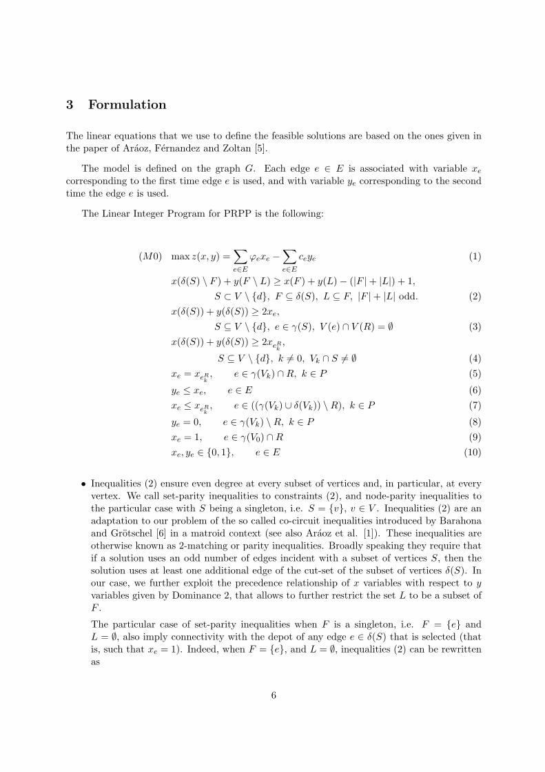
3 Formulation
The linear equations that we use to define the feasible solutions are based on the ones given inthe paper of Araoz, Fernandez and Zoltan [5].
The model is defined on the graph G. Each edge e ∈ E is associated with variable xe
corresponding to the first time edge e is used, and with variable ye corresponding to the secondtime the edge e is used.
The Linear Integer Program for PRPP is the following:
(M0) max z(x, y) =∑e∈E
ϕexe −∑e∈E
ceye (1)
x(δ(S) \ F ) + y(F \ L) ≥ x(F ) + y(L)− (|F |+ |L|) + 1,S ⊂ V \ {d}, F ⊆ δ(S), L ⊆ F, |F |+ |L| odd. (2)
x(δ(S)) + y(δ(S)) ≥ 2xe,
S ⊆ V \ {d}, e ∈ γ(S), V (e) ∩ V (R) = ∅ (3)x(δ(S)) + y(δ(S)) ≥ 2xeR
k,
S ⊆ V \ {d}, k 6= 0, Vk ∩ S 6= ∅ (4)xe = xeR
k, e ∈ γ(Vk) ∩R, k ∈ P (5)
ye ≤ xe, e ∈ E (6)xe ≤ xeR
k, e ∈ ((γ(Vk) ∪ δ(Vk)) \R), k ∈ P (7)
ye = 0, e ∈ γ(Vk) \R, k ∈ P (8)xe = 1, e ∈ γ(V0) ∩R (9)xe, ye ∈ {0, 1}, e ∈ E (10)
• Inequalities (2) ensure even degree at every subset of vertices and, in particular, at everyvertex. We call set-parity inequalities to constraints (2), and node-parity inequalities tothe particular case with S being a singleton, i.e. S = {v}, v ∈ V . Inequalities (2) are anadaptation to our problem of the so called co-circuit inequalities introduced by Barahonaand Grotschel [6] in a matroid context (see also Araoz et al. [1]). These inequalities areotherwise known as 2-matching or parity inequalities. Broadly speaking they require thatif a solution uses an odd number of edges incident with a subset of vertices S, then thesolution uses at least one additional edge of the cut-set of the subset of vertices δ(S). Inour case, we further exploit the precedence relationship of x variables with respect to yvariables given by Dominance 2, that allows to further restrict the set L to be a subset ofF .
The particular case of set-parity inequalities when F is a singleton, i.e. F = {e} andL = ∅, also imply connectivity with the depot of any edge e ∈ δ(S) that is selected (thatis, such that xe = 1). Indeed, when F = {e}, and L = ∅, inequalities (2) can be rewrittenas
6

x(δ(S) \ F ) + y(F \ L) ≥ xe + 1− 1 ≡x(δ(S))− xe + ye ≥ xe ≡
x(δ(S)) + ye ≥ 2xe (11)
We denote this particular case as parity-connectivity inequalities.
• Inequalities (3) and (4) ensure connectivity with the depot of any edge e ∈ γ(S) that isselected (that is, such that xe = 1). By Dominance 2 we do not need to check connectivitywhen ye = 1, and by Dominance 3 for the edges in Ck we only need to check for eRk . Theseinequalities are referred to as connectivity inequalities. Inequalities (3) and (4), togetherwith inequalities (2), guarantee that the solution to the model define Eulerian circuits.
• Equalities (5) correspond to Dominance 3.
• Inequalities (6) correspond to Dominance 2.
• Inequalities (7) are also implied by Dominance 3 (see Remark 2.7).
• Equalities (8) correspond to Preprocessing 1.
• Equalities (9) correspond to Preprocessing 2.
• Binary conditions (10) correspond to Dominance 1.
4 Algorithm
In this section we describe the algorithm that we apply to solve PRPP. Different types of routingproblems are frequently modeled using families of constraints that have an exponential numberof inequalities. In these cases, the models are too big to be given to any solver, even for obtainingLP bounds when integrality constraints are relaxed. Several approaches have been proposed andused for this type of systems, among which Branch and Cut is probably the most common one.
In the case of the proposed model for PRPP, the families of constraints (2), (3), (4) have anexponential number of inequalities. Hence, our goal is to find a relatively small subset of theseinequalities that determines the optimal vertex. The algorithm that we propose has two phases.Both phases are based on an iterative scheme like the one depicted in Figure 1. The differencebetween the two phases is the type of relaxation to PRPP that is considered at each iteration.Both relaxations are constraint relaxations of PRPP in the sense that only a subset of constraints(2), (3), (4) are considered. In the first phase we additionally relax integrality constraints onthe variables, so that the problem that is solved at each iteration is an LP problem, whereasin the second phase, integrality conditions on the variables are kept, so that the relaxation ofPRPP is an Integer Problem (IP) with binary variables. For ease of presentation in Figure 1,within the same phase, we denote RM0 to the input and RMr to the problem that is solved atiteration r of the corresponding phase. The input of the first phase will be described in the next
7
subsection. The input of the second phase is the problem that is solved in the last iteration ofthe first phase strengthened with the integrality conditions of the variables.
In both phases we solve exactly the separation problem to generate violated cuts associatedwith constraints (2), (3), (4), when they exist. Each of the two phases terminates when at agiven iteration there are no more cuts violated by the solution to the current relaxation or ifoptimality of the best solution found so far is proven. When the first phase terminates thealgorithm enters the second phase, and the algorithm ends when the second phase terminates.Let z denote the upper bound, and let bestxy be the best solution found so far, with value z,at the end of an iteration. Optimality is proven when z − z = 0. In this case, bestxy is theoptimal solution. At the end of the first phase, when optimality has not been proven, integralityconditions are posed on the variables of the current LP, and the algorithm enters the secondphase. A scheme of a phase of the algorithm is given in Figure 2. We next describe its maincomponents.
CutProcedure(r = 0; z; z; bestxy)
1. endphase= false;
2. while endphase= false do:
3. begin
(a) Find a solution (x∗, y∗) of RMr; z(x∗, y∗) denotes its associated cost;
(b) if z > z(x∗, y∗) then z = z(x∗, y∗);
(c) if(x∗, y∗) is feasible to PRPP thenbestxy= (x∗, y∗); z = z; endphase= true;
else
i. Identify inequalities of types (2), (3), (4) violated by (x∗, y∗);
ii. Add the valid inequalities identified in step (3.(c)i.) to RMr;
iii. Compute the 3T heuristic solution (xh, yh); z(xh, yh) denotesits associated cost (only in the first phase);
iv. if z < z(xh, yh) then z = z(xh, yh); bestxy = (xh, yh);
v. if (z = z) or (no inequality has been added in step (3.(c)ii.))then endphase=true;
vi. r := r + 1
4. end (3)
5. output(RMr; z; z; bestxy)
Figure 2: Scheme of each phase of the Algorithm
Observe that the two phase algorithm that we propose can be seen as a branch-and-cutalgorithm in which (in phase 2) we resort to a general purpose solver for deciding the strategieson the branching variables and the selection of subproblems. In this algorithm we only generatecuts associated with inequalities (2), (3) and (4) at the root node (phase 1) or when some integersolution is obtained. At the rest of the nodes of the search tree (phase 2) the general purposesolver possibly generates Gomory cuts that are not included in our model.
8

4.1 Initial LP Relaxation
The cutting plane algorithm starts with the following LP:
(LPM0)
max z(x, y) =∑e∈E
ϕexe −∑e∈H
ceye
x(δ(v)) + ye ≥ 2xe, v ∈ V, e ∈ δ(v).x(δ(Vk)) + y(δ(Vk)) ≥ 2xeR
k, k ∈ P \ {0}
xe = xeRk, e ∈ γR(Vk) and k ∈ P \ {0}
ye ≤ xe, e ∈ Exe ≤ xeR
k, e ∈ ((γ(Vk) ∪ δ(Vk)) \R), k ∈ P
xe = 1, e ∈ γ(V0) ∩R0 ≤ xe ≤ 1, 0 ≤ ye ≤ 1, e ∈ E
This initial program, in which integrality conditions (10) are relaxed, has the same functional(1) and all the inequalities (5)-(9) of M0. LPM0 only includes a subset of inequalities of type(2), namely δ(v) + ye ≥ 2xe, v ∈ V, e ∈ δ(v), which are the parity-connectivity inequalitiesassociated with singletons S = {v}, v ∈ V . LPM0 does not include any inequality (3), but itincludes the subset of the connectivity inequalities (4) associated with the sets S = Vk, e = eRk .
It is important to note that, since some of the original constraints are omitted, the solutionsto this system need not be feasible to the PRPP even if they were integer.
5 Separation of Cuts
At a given iteration of the algorithm the step that solves exactly the separation problem forthe relaxed inequalities consists of two parts: first, we look for violated inequalities of type(2), and second, we look for violated inequalities of type (3) and (4). Throughout Gx∗,y∗ =(V,Ex∗,y∗) denotes the support graph of the current solution (x∗, y∗), obtained from the graphG by eliminating all edges in E with x∗e = 0. Our separation algorithms for inequalities (2), willbe presented first for general co-circuit inequalities with generic variables x. ThenGx∗ = (V,Ex∗)will denote the support graph with respect to a given vector x∗.
5.1 Finding violated inequalities of type (2)
First, we give exact separation algorithms for two subsets of inequalities (2), namely i) node-parity inequalities, that is S = {v}, v ∈ V and general subsets F ⊆ δ(v), |F | odd, and, ii)parity-connectivity inequalities. Then, we give the exact separation for the general case.
9
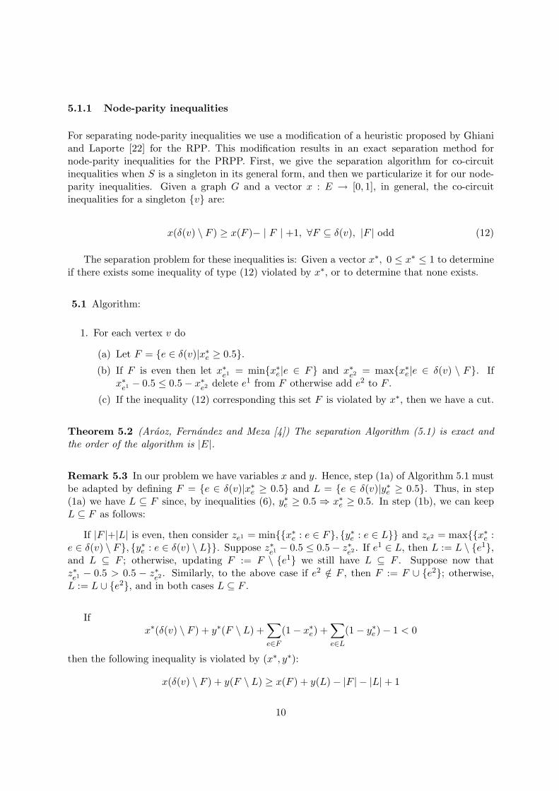
5.1.1 Node-parity inequalities
For separating node-parity inequalities we use a modification of a heuristic proposed by Ghianiand Laporte [22] for the RPP. This modification results in an exact separation method fornode-parity inequalities for the PRPP. First, we give the separation algorithm for co-circuitinequalities when S is a singleton in its general form, and then we particularize it for our node-parity inequalities. Given a graph G and a vector x : E → [0, 1], in general, the co-circuitinequalities for a singleton {v} are:
x(δ(v) \ F ) ≥ x(F )− | F | +1, ∀F ⊆ δ(v), |F | odd (12)
The separation problem for these inequalities is: Given a vector x∗, 0 ≤ x∗ ≤ 1 to determineif there exists some inequality of type (12) violated by x∗, or to determine that none exists.
5.1 Algorithm:
1. For each vertex v do
(a) Let F = {e ∈ δ(v)|x∗e ≥ 0.5}.(b) If F is even then let x∗e1 = min{x∗e|e ∈ F} and x∗e2 = max{x∗e|e ∈ δ(v) \ F}. If
x∗e1 − 0.5 ≤ 0.5− x∗e2 delete e1 from F otherwise add e2 to F .
(c) If the inequality (12) corresponding this set F is violated by x∗, then we have a cut.
Theorem 5.2 (Araoz, Fernandez and Meza [4]) The separation Algorithm (5.1) is exact andthe order of the algorithm is |E|.
Remark 5.3 In our problem we have variables x and y. Hence, step (1a) of Algorithm 5.1 mustbe adapted by defining F = {e ∈ δ(v)|x∗e ≥ 0.5} and L = {e ∈ δ(v)|y∗e ≥ 0.5}. Thus, in step(1a) we have L ⊆ F since, by inequalities (6), y∗e ≥ 0.5 ⇒ x∗e ≥ 0.5. In step (1b), we can keepL ⊆ F as follows:
If |F |+|L| is even, then consider ze1 = min{{x∗e : e ∈ F}, {y∗e : e ∈ L}} and ze2 = max{{x∗e :e ∈ δ(v) \ F}, {y∗e : e ∈ δ(v) \ L}}. Suppose z∗e1 − 0.5 ≤ 0.5− z∗e2 . If e1 ∈ L, then L := L \ {e1},and L ⊆ F ; otherwise, updating F := F \ {e1} we still have L ⊆ F . Suppose now thatz∗e1 − 0.5 > 0.5 − z∗e2 . Similarly, to the above case if e2 /∈ F , then F := F ∪ {e2}; otherwise,L := L ∪ {e2}, and in both cases L ⊆ F .
Ifx∗(δ(v) \ F ) + y∗(F \ L) +
∑e∈F
(1− x∗e) +∑e∈L
(1− y∗e)− 1 < 0
then the following inequality is violated by (x∗, y∗):
x(δ(v) \ F ) + y(F \ L) ≥ x(F ) + y(L)− |F | − |L|+ 1
10

5.1.2 Parity-connectivity inequalities
For separating parity-connectivity inequalities we first obtain the tree of min-cuts (see, forinstance, [23]) of the support graph Gx∗,y∗ , after assigning to each edge e a capacity of value(x∗e + y∗e). Then, the parity-connectivity inequalities are separated exactly with a very simplealgorithm: For each edge e = {u, v} ∈ E we determine the cut δ(S) in Gx∗,y∗ , that separatesv and u, which is minimum relative to the assigned capacities. If the value of this min-cut isless than 2xe then the following inequality is violated by (x∗, y∗): x(δ(S)) + y(δ(S)) ≥ 2xe. Theorder of this algorithm is dominated by that of the algorithm to obtain the cut tree, which isO(|V |4).
5.1.3 General case
Set-parity inequalities (2) can be separated exactly for general sets S and F ⊂ S, |F | odd inpolynomial time. In [24] Grotschel and Holland [24] propose an algorithm for separating Set-parity inequalities, which was applied in the context of Perfect 2-Matchings. Belenguer andBenavent [8] and Benavent et al. [12] have used this exact algorithm in the context of arc-routing problems. Other authors have considered heuristics to separate some particular cases.For instance, Ghiani and Laporte [22] proposed a heuristic for finding node-parity inequalitiesin the context of the RPP. The separation algorithm of [24] requires to apply the Padberg-Raoalgorithm [26] to an ad hoc graph, that contains more nodes and edges than the support graphof the given solution. In particular, if Gx∗ = (V,Ex∗) denotes the support graph of a givenvector x∗, 0 ≤ x∗e ≤ 1 e ∈ E, the ad hoc graph used in the algorithm of [24] has |V |+K verticesand |Ex∗ |+K edges, where K denotes the number of non integer components of x∗. Thus, theorder of the algorithm is (O
((|V |+ |E|)4
)) (see [24]). The exact separation algorithm that we
use in this work has been proposed recently by Araoz, Fernandez and Meza [4]. This separationalgorithm requires to find the min-cut tree of the original support graph of Gx∗ relative to adhoc capacities on the edges, and is of order (O(|V |)4). Next we present the separation algorithmof Araoz, Fernandez and Meza [4] for co-circuit inequalities in their general form and then weparticularize for the case of our inequalities (2) with x and y variables. Given a graph G and avector x : E → [0, 1], the general form of inequalities (2) for a subset of vertices S ⊂ V is:
x(δ(S) \ F ) ≥ x(F )− | F | +1, ∀F ⊆ δ(S), |F | odd,
that can be rewritten as
∑e∈δ(S)\F
xe +∑e∈F
(1− xe) ≥ 1, ∀F ⊆ δ(S), |F | odd, (13)
For a given vector x∗, the separation problem for inequalities (13) is to find S∗ ⊂ V ,F ∗ ⊆ δ(S∗), |F ∗| odd such that the associated inequality (13) is violated by x∗, or to provethat no such inequality exists.
For separating inequalities (13), each edge in Ex∗ is assigned a capacity given by
he = min{x∗e, 1− x∗e}.
11

We partition Ex∗ , Ex∗ = E< ∪ E> so that an edge e belongs to E< (resp. E>) if and onlyif its capacity is given by x∗e (resp. 1 − x∗e). Values 0.5 are assigned arbitrarily to E< or toE>. We say that a vertex v ∈ V is odd> if and only if |δE>(v)| is odd; otherwise we say thatv is even>. By extension, we say that a subset S ⊆ V is odd> if it contains an odd number ofvertices labelled odd, i.e. |{v ∈ S : v is odd}| is odd.
Lemma 5.4 (Araoz, Fernandez and Meza [4])
(a) For S ⊂ V , |δE>(S)| is odd if and only if S is odd>.
(b) V is even>.
Lemma 5.5 (Araoz, Fernandez and Meza [4]) Let S be a vertex subset, the following two pro-prieties hold:
(a) When S is odd> then a subset F , |F | odd, that minimizes the value of the left hand sideof constraint (13) is given by F = δE>(S). The minimum value of the left hand side ofthe inequality is then given by h(δ(S)).
(b) When S is even>, a subset F ⊆ δ(S), |F | odd, with minimum value of the left hand sideof constraint (13) can be obtained as follows. If x∗e1
− (1 − x∗e1) < (1 − x∗e2) − x∗e2
thenF = δE>(S) \ {e1}, with x∗e1 = min{x∗e : e ∈ δE>(S)}. Otherwise, F = δE>(S)∪{e2}, withe2 such that x∗e2 = max{x∗e : e ∈ δ(S) \ δE>(S)}. The minimum value of the left hand sideof the inequality is given by h(δ(S)) + min{x∗e1
− (1− x∗e1), (1− x∗e2)− x∗e2
}.
Throughout for a given cut-set δ(S), e1 and e2 denote arbitrarily chosen edges such thatx∗e1 = min{x∗e : e ∈ δE>(S)} and x∗e2 = max{x∗e : e ∈ δ(S) \ δE>(S)}. Lemma 5.5 indicates thatfor a given vector x∗, the smallest value of the left hand side in constraint (13) may correspondi) to an odd> set S with F = δE>(S), or ii) to an even> set S, with a modified set F defined asindicated in Lemma 5.5(b).
Hence, in order to solve the separation problem for a given vector x∗ we must identifyboth the odd> set S with minimum capacity h(δ(S)), and the even> set S that minimizesh(δ(S)) = h(δ(S)) + min{x∗e1
− (1 − x∗e1), (1 − x∗e2) − x∗e2
}. The following well-known result ofPadberg and Rao [26] indicates how to identify the odd> set S with minimum capacity h(δ(S)).First, we give some additional notation.
Suppose that each vertex v ∈ V is assigned some label λ with two possible values (odd oreven). By extension, subsets of vertices also are assigned labels. In particular, for U ∈ V , λ(U)is odd iff U contains an odd number of vertices labelled odd. For S ⊂ V , (S : V \ S) is analternative way of denoting the cut-set δ(S).
Lemma 5.6 (Padberg and Rao [26]) Let G = (V,E) and ce ≥ 0 for all e ∈ E. Let V = V0 ∪ V1
where V1 is a nonempty set of nodes of G with odd label, V0 is the set of nodes with even labeland λ(V ) is even. Let (M : V \M) be a minimum cut-set with respect to all pairs of odd labellednodes in G. Then, there exists an odd minimum cut-set (X : V \X) in G such that X ⊆M orX ⊆ V \M holds.
12
Let ce = he, for all e ∈ E, and V1 = {v ∈ V : v is odd>}. We assume that V1 6= ∅, sinceotherwise no odd> set exists. Since V is even> we obtain the following result.
Corollary 5.7 (Araoz, Fernandez and Meza [4]) Let Gx∗ = (V,Ex∗) and he ≥ 0 for all e ∈ Ex∗.Let δ(M) be a minimum cut-set with respect to all pairs of odd> nodes in Gx∗. Then there existsan odd> set S with minimum capacity h(δ(S)) such that S ⊆M or S ⊆ V \M holds.
As it is well-known, Lemma 5.6 implies that a minimum odd cut-set will be one of the cutsthat define the tree of min-cuts of all pairs of odd labelled vertices. Thus, a minimum oddcut-set will also be one of the cuts that define the tree of min-cuts of all pairs of nodes. Hence,Corollary 5.7 implies that an odd> set S with a minimum capacity h(δ(S)) will be one of thecuts that define T , the tree of min-cuts of all pairs of vertices of Gx∗ relative to the capacitiesvector h.
We next turn our attention to how to identify an even> set S that minimizes (h)(δ(S)) =h(δ(S)) + min{x∗e1
− (1− x∗e1), (1− x∗e2)− x∗e2
}.
Lemma 5.8 (Araoz, Fernandez and Meza [4]) Let δ(S) be a cut-set with S even>.
a) Let e ∈ δ(S) ∩ E> be such that h(δ(S)
)− (1 − xe) + xe < 1. Then, there exist a cut-
set δ(S) associated with one edge of T , e ∈ δ(S), and F ⊂ δ(S), |F | odd, such that thecorresponding inequality (13) is violated by x∗.
b) Let e ∈ δ(S) ∩ E< be such that h(δ(S)
)− xe + (1 − xe) < 1. Then, there exist a cut-
set δ(S) associated with one edge of T , e ∈ δ(S), and F ⊂ δ(S), |F | odd, such that thecorresponding inequality (13) is violated by x∗.
The above lemma implies that if there exist an even> set S, and a subset F ⊆ δ(S), |F | odd,such that its associated inequality (13) is violated by x∗, then, there exists a cut-set in T (thetree of min-cuts of all pairs of vertices of Gx∗ relative to the capacities vector h) such that itsassociated inequality (13) is violated by x∗. The result of Lemma 5.8 plays an important role.Due to this result, if there exist violated inequalities (13), one such inequality will be associatedto a cut-set of T . Hence, Lemma 5.8 together with Corollary 5.7 guarantee that the separationproblem can be solved with order no greater than the procedure to find the min-cuts tree T .
The algorithm that we propose starts building T , the tree of min-cuts of all pairs of verticesof Gx∗ relative to the capacities vector h. Then the edges in T are explored in turn until amin-cut is found for which the associated inequality (13) is violated, or until all the edges in Thave been considered. Each considered min-cut δ(Si) is associated with a vertex set Si, whichis is either odd> or even>. In the first case, we only have to check if its capacity is smaller thanone. If so, F = δE>(Si). When Si is even>, the associated set F will be F = δE>(Si) \ {e1}when x∗e1
− (1 − x∗e1) < (1 − x∗e2) − x∗e2
, or F = δE>(Si) ∪ {e2}, otherwise. Once F is defined,we have to check if F together with Si it defines a violated inequality (13). The algorithm is asfollows:
13
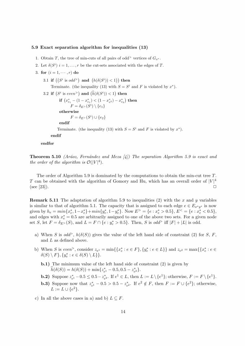
5.9 Exact separation algorithm for inequalities (13)
1. Obtain T , the tree of min-cuts of all pairs of odd> vertices of Gx∗ .
2. Let δ(Si) i = 1, . . . , r be the cut-sets associated with the edges of T .
3. for (i = 1, · · · , r) do
3.1 if((Si is odd>
)and
(h(δ(Si)) < 1
))then
Terminate. (the inequality (13) with S = Si and F is violated by x∗).
3.2 if(Si is even>
)and
(h(δ(Si)) < 1
)then
if(x∗e1
− (1− x∗e1) < (1− x∗e2)− x∗e2
)then
F = δE>(Si) \ {e1}otherwise
F = δE>(Si) ∪ {e2}endif
Terminate. (the inequality (13) with S = Si and F is violated by x∗).
endif
endfor
Theorem 5.10 (Araoz, Fernandez and Meza [4]) The separation Algorithm 5.9 is exact andthe order of the algorithm is O(|V |4).
The order of Algorithm 5.9 is dominated by the computations to obtain the min-cut tree T .T can be obtained with the algorithm of Gomory and Hu, which has an overall order of |V |4(see [23]). 2
Remark 5.11 The adaptation of algorithm 5.9 to inequalities (2) with the x and y variablesis similar to that of algorithm 5.1. The capacity that is assigned to each edge e ∈ Ex∗y∗ is nowgiven by he = min{x∗e, 1−x∗e}+min{y∗e , 1−y∗e}. Now E> = {e : x∗e > 0.5}, E< = {e : x∗e < 0.5},and edges with x∗e = 0.5 are arbitrarily assigned to one of the above two sets. For a given nodeset S, let F = δE>(S), and L = F ∩ {e : y∗e > 0.5}. Then, S is odd> iff |F |+ |L| is odd.
a) When S is odd>, h(δ(S)) gives the value of the left hand side of constraint (2) for S, F ,and L as defined above.
b) When S is even>, consider ze1 = min{{x∗e : e ∈ F}, {y∗e : e ∈ L}} and ze2 = max{{x∗e : e ∈δ(S) \ F}, {y∗e : e ∈ δ(S) \ L}}.
b.1) The minimum value of the left hand side of constraint (2) is given byh(δ(S)) = h(δ(S)) + min{z∗e1 − 0.5, 0.5− z∗e2}.
b.2) Suppose z∗e1 −0.5 ≤ 0.5−z∗e2 . If e1 ∈ L, then L := L\{e1}; otherwise, F := F \{e1}.b.3) Suppose now that z∗e1 − 0.5 > 0.5 − z∗e2 . If e2 /∈ F , then F := F ∪ {e2}; otherwise,
L := L ∪ {e2}.
c) In all the above cases in a) and b) L ⊆ F .
14

FIGURE 3 HERE
Figure 3: Fractional solution that cannot be separated by inequalities (2), (3), (4).
5.2 Finding violated inequalities of type (3) or (4)
For separating any of the inequalities (3) and (4) again we use the tree of min-cuts of the graphGx∗ with the capacities given by x∗e + y∗e as defined in 5.1.2. Then, we use the exact algorithmof Belenguer and Benavent [8, 9]. The algorithm does the following:
For each edge e = {u, v} ∈ E with u and v different from the depot and x∗e > 0, the minimumcut δ(S) such that e ∈ γ(S) is easily obtained from the min-cut tree. If the value of the min cutis smaller than 2x∗e then the following inequality is violated by (x∗, y∗): x(δ(S))+y(δ(S)) ≥ 2xe.
5.3 Cut generation strategy
The exact separation procedure for node-parity inequalities has order O(|E|), whereas the restof the separation procedures are of order O(|V |4) since they require to obtain the min-cut treerelative to different capacity functions. The separation procedures for parity-connectivity in-equalities and for connectivity inequalities operate on the min-cut tree associated with capacitiesx∗e + y∗e , whereas the separation procedure for the general co-circuit inequalities operates on themin-cut tree associated with capacities min{x∗e, 1 − x∗e} + min{y∗e , 1 − y∗e}. Since for parity-connectivity inequalities and for connectivity inequalities the same min-cut tree is used, at eachiteration of the first phase of Algorithm 2 we always apply the separation procedures for node-parity, parity-connectivity, and connectivity inequalities. On the contrary, we only apply theexact separation procedure for the general case of inequalities (2) when no violated inequalityof any of the other types has been found.
5.4 Other cuts
Given that the procedures that we apply to separate inequalities (2), (3) and (4) are exact, whenno cuts associated with these constraints are violated by the current solution, then either thesolution is optimal or it necessarily has fractional values. Hence, there are indeed additionalinequalities, other from the ones in system (2)-(8), needed to characterize the convex hull offeasible solutions to PRPP. Figure 3 gives an example of a fractional solution that satisfiesconstraints (5)-(8) and does not violate any inequality (2), (3), (4). When the current relaxationgives such a point, and the fractional part of some basic variable is above some threshold value,we resort to Gomory cuts [20] to cutoff such a solution.
15

6 Lower bounds
Next we describe how we obtain feasible solutions, and thus lower bounds for the problem.We have not designed an ad hoc heuristic that exploits the specific characteristics of PRPP.Instead, we transform PRPP into a RPP and then we apply the 3T heuristic of Fernandez,Meza, Garfinkel and Ortega [18], which gives good results on RPP instances.
The heuristic that we use at each iteration to obtain a feasible solution is the following:
1. Let (x∗, y∗) be the solution of the current linear programming relaxation.
2. Transform the PRPP into a RPP. The graph of the RPP will be the original graph Gof PRPP plus fictitious vertex d′ and edge {d, d′}. Edge {d, d′} is defined as required toguarantee that the solution passes through the depot. All other edges of PRPP with valuex∗e greater or equal to ε are also defined as required edges for RPP (ε is a parameter). Thecost of edge {d, d′} is zero, and any other edge e inherits its cost ce from PRPP.
3. Find a feasible solution to RPP with the 3T heuristic of Fernandez, Meza, Garfinkel andOrtega [18].
4. The feasible solution to PRPP results from eliminating the parallel edges {d, d′} from thefeasible solution to RPP obtained in step 3.
In the computational experiments, the 3T heuristic is applied twice at each iteration of thefirst phase: the first time we use ε = 0.9. That is, in step 1 we include in the graph of the RPPall the edges with x∗e > 0.9. The second time that we apply the heuristic we use ε = 0.8 andinclude in the graph of the RPP all the edges such that be − 2ce > 0 with x∗e > 0.8.
7 Computational Experiments
In order to evaluate the performance of the proposed algorithm we have run a series of com-putational experiments. We next describe such experiments and give the obtained numericalresults. Programs have been coded in C using CPLEX 7.0 library for the solution of the LPrelaxations of the first phase and for the solution of the Integer Problems of the second phase.Default parameters have been used.
All instances were run on a Sun ULTRA 10, model 440, 1x440 MHZ, 1GB DRAM. Since thereare no available PRPP benchmark instances, we have generated 118 PRPP instances from wellknown sets of benchmark RPP instances. The 118 RPP benchmark instances are divided in fivegroups. The first group contains two problems, ALBAIDAA and ALBAIDAB, obtained fromthe Albaida, Spain Graph (see Corberan and Sanchis [14]). The second group contains the 24instances (problems labeled P) of Christofides et al. [10]. The last three groups contain instancesfrom Hertz et al [25]: 36 instances with vertices of degree 4 and disconnected required edgesets (labeled D), 36 grid instances (labeled G), and 20 randomly generated instances (labeledR). Table 1 depicts information on these instances, that have been grouped according to their
16
characteristics and to their sizes. In particular, column under #inst. gives the number ofinstances in the group, columns under |V | and |E| give, respectively, the number of vertices andedges; column under |R| gives the number of edges in the set R, and the last column under|P | gives the number of connected components in the graph GR. In all columns when all theinstances of the group did not have the same values, the minimum and maximum values in thegroup are given.
In all cases the depot has been taken as vertex 1, and we have kept the cost function cfrom the original RPP instance. The profits have been generated as follows (U[a,b] denotes theinteger uniform distribution in the interval [a,b]):
• be ∈ U[ce, 3ce], if e is a required edge of the RPP instance.
• be ∈ U[0, ce], if e is a non-required edge of the RPP instance.
The results are summarized in Table 2, although detailed results for each of the instances canbe found in http://www-eio.upc.es/ elena/index.html. Columns 2-12 give results correspondingto the first phase. They have been divided in several blocks: Columns 2-4 refer to the LPrelaxation and Columns 5-7 to the heuristic. Column under #LP gives the number of LPiterations in the first phase, and Columns 9-12 give information on the cuts generated. Inparticular, the column under gapRL, gives the average percent gap at the end of phase 1 withrespect to the optimal solution of the upper bound obtained with the LP relaxation. That is,if zopt denotes the value of the optimal solution to the problem, and zRL denotes the valuesof the LP relaxation at the end of the first phase, the entries of the column gapRL give theaverage values of the deviations 100 ∗ zRL−zopt
zopt, over all the instances in each group. Columns
under #optRL, and tRL give, respectively, the number of instances in the group that have beenoptimally solved with the LP relaxation; and the average cpu-time in seconds.
Similarly, the next three columns under gapH , #optH , and tH give the average percent gapwith respect to the optimal solution of the lower bound obtained with the heuristic (average valueof the deviations 100 ∗ zopt−zH
zopt), the number of instances in the group that have been optimally
solved with the heuristic, and the average cpu-time in seconds, respectively. The following fourcolumns, under v-par, par-conn, S-par and conn, depict the average number of generated cuts ofnode-parity (12), parity-connectivity (11), co-circuit for the general case (2), and connectivity(3)-(4), respectively. The last three columns in the table give results corresponding to the secondphase. The column under #IP gives the average number of iterations performed in the secondphase, which corresponds to the average number of integer problems that had to solved. Columnunder #nod shows the average number of nodes that were explored in the search tree of each ofthe integer problems that had to be solved, and, finally, column tIP gives the total cpu-time inseconds required by the second phase of the algorithm.
In our opinion, the obtained results are very good. As can be seen the optimal solution tothe LP relaxation gave the optimal value of the problem for 94 out of the 118 instances. In 87 ofthese instances optimality could be proven since the solution that gave the bound was alreadyinteger. In general, the percent deviation of the LP relaxation from the optimal solution atthe end of the first phase is very small, with fifteen instances (in addition to the 94 ones abovementioned) with a percent gap smaller than 1%. There are four instances with a percent gap
17

between 1% and 2%; three instances with a percent gap between 2% and 5%; one more instancefor which this percent gap is between 5% and 10% (in fact, slightly smaller than 7%); and, onlyone instance (in group PG64) for which this percent gap was over 10% (quite surprisingly, thisinstance was optimally solved by the heuristic).
Despite its simplicity, the behavior of the heuristic is also very good, since it gave the optimalsolution in 92 out of the 118 instances. In most of the cases, the percent deviations from theoptimal solution were larger in magnitude than those of the upper bounds, but again there isonly one instance (in PP) where the percent gap between the heuristic and optimal solutions isabove 10%.
Usually, the number of LP iterations in the first phase of the algorithm is quite small. For86 out of the 118 instances this number does not exceed 20, and only 10 instances requiredmore than 100 iterations to terminate the first phase. As could be expected, the instancesthat required more iterations are the ones with a larger number of connected components inthe graph induced by the edges in the set R. To some extent the difficulty for solving theinstances is also reflected on the number of cuts that were added: both in the total number ofcuts and on the number of cuts per iteration. In our opinion the number of generated cuts issmall taking into account the difficulty of the problems. In general, the parity-connectivity cuts(11), followed by connectivity cuts (3)-(4), are more frequent than general co-circuit cuts (2)and node-parity cuts (12). Taking into account our strategy for generating cuts, according towhich the general co-circuit inequalities are only generated when none of the other cuts wereobtained, these figures illustrate the important role of the general co-circuit inequalities in theperformance of our algorithm. In fact, a previous version of the algorithm where the exactalgorithm for the separation of the general case of co-circuit inequalities was not used, andthe only co-circuit inequalities that were generated were vertex-parity and parity-connectivity,was able to optimally solve in the first phase 55 instances, instead of the 94 instances that areoptimally solved when the exact separation algorithm for the general case is also applied.
However, the increase on the cpu-time due to the application of the exact separation pro-cedure is quite small, and the efficiency of the algorithm can be appreciated in the requiredcpu-times. The distribution of the cpu-times needed to solve the LP relaxation is the following:36 instances required less than 1 second; for 38 instances the cpu-time was in the interval [1, 10);for 18 instances the cpu-time was in the interval [10, 60); for 7 instances the cpu-time was in theinterval [60, 120). Nineteen instances required more than 120 seconds of cpu-time, of which sixrequired more than 600 seconds of cpu-time. Quite surprisingly, the cpu-time requirements ofthe heuristic were in quite a few cases higher than those of the iterative LP solver.
The results of the last three columns of Table 2 indicate that in most cases the consideredinstances could be optimally solved efficiently. Note that with our solution method the percentdeviation between the upper and lower bounds at the end of the first phase is only a reliableindicator of “how far” we are from optimality for the current model. However, there mightbe inequalities of types (2), (3),(4) which have not been generated so far, which are necessaryto characterize the optimal solution to the original problem. So, although this is not likely tohappen, even if the percent gap at the end of the first phase is small it might be necessary tosolve more than one integer problem. Of the 31 instances that were not solved optimally in
18

the first phase, 15 required only one iteration of the second phase (that is, the solution of oneinteger problem), 9 required two iterations, 3 required five iterations, one required 10 iterations,and the remaining instance required the solution of 13 integer problems. In our opinion, theindicator of the difficulty for solving a given instance is the number of nodes that were exploredin the second phase. It is worth noting that 16 of the 31 instances that entered the second phasecould be optimally solved without exploring any node of any search tree. This means that theoptimal solution was found in the presolve phase of the search, which means that the cuts usedby CPLEX at the root node (Gomory cuts, etc.) together with the cuts that we had generatedin the first phase were enough as to characterize an optimal vertex. For the remaining instances,the total number of nodes that had to be solved during all the iterations of the second phaseis smaller than 10 for seven instances, in the interval [10, 20) for three instances, in the interval[20, 100) for two instances, and the remaining three instances required to explore more than 100nodes to be optimally solved. As could be expected these three instances are large ones: one inthe group PD100, and two in PG100.
In general, the cpu-times required for the second phase of our algorithm are small. Out ofthe 31 instances that entered this second phase, nine required less than one second; for eightinstances this time was in the interval [1, 10); for six instances the cpu-time was in [10, 60); thecpu-time for one instance was in [60, 120); and, three more instances required a cpu-time inthe interval [120, 160). Only four instances required more than 600 seconds of cpu-time, one inPD100, one in PG64, and two in PG100. Out of these, only the instance in PD100 requiredmore than 1,200 seconds of cpu to be optimally solved (nearly 12,000 seconds).
The results depicted in Table 2 assess the good behavior of the selected algorithm. In ouropinion this is basically due to the efficiency of the first phase where in most cases a quitesmall subset of inequalities is sufficient for finding an optimal solution was found. In the caseswhen this subset was not complete, just a few additional inequalities were needed and, thus, thecomputational burden of the second phase was small. For the instances that entered the secondphase, the average ratio between “cpu-time of the first phase” over “cpu-time of the secondphase” was over 16, thus indicating the primacy of the first phase over the second one. Oneadditional positive aspect of our algorithm is its ease of implementation.
Since in [5] it was proven that the RPP is a particular case of the PRPP, we have alsoperformed a second series of computational experiments with RPP benchmark instances. Giventhat the focus of this work is the PRPP and not the RPP, the goal of these experiments is toillustrate how, in fact, of our solution algorithm for PRPP can also be used efficiently for solvingspecific RPP instances, and not to compete with the most effective ad hoc methods for the RPP[11, 18, 22]. To this end, we have again considered the same set of RPP benchmark instancesused for the first series of experiments, that have been considered in several works for the RPP(see, for instance [11, 18, 22]). As can be seen in Table 1 their sizes go up to 100 vertices, 4950edges and 200 R-sets, although they are not the largest RPP instances we are aware of with upto 1000 vertices, 3000 edges and 200 R-sets (see Corberan, Plana and Sanchis [13]). From [5]we know that we can transform RPP instances into equivalent PRPP instances by i) keeping inPRPP the cost function c of RPP, and ii) by defining a profit function b in PRPP that assignshigh enough profits to the edges that are required in RPP and zero profit for the edges thatare non-required in RPP. According to this, for the second series of experiments we have set
19

be = 1000ce,∀e ∈ ER, and be = 0,∀e ∈ E \ ER.
The results with this second set of instances are summarized in Table 3. The meaning ofthe entries is the same as before. As can be seen the obtained results are very good. Despitethe fact that neither the model that we use nor our algorithm exploit explicitly the structure ofRPP instances, the results that we have obtained are nearly as good in terms of both the qualityof the obtained solutions and the cpu-time requirements as the best published results for thesame sets of benchmark instances [11, 18, 22]. In particular, the heuristic provided the optimalsolution for 117 of the 118 instances. We attribute the good behavior of the heuristic to thefact that it is, in fact, an adaptation of a heuristic that has been designed for RPP instances.In 76 of the instances, we could prove the optimality of the heuristic solution because the valueof the LP relaxation at the end of the first phase was optimal (0% percent gap between theupper and the lower bounds). For the remaining 42 instances the percent gaps between theupper bound given by the LP relaxation and the optimal value was always smaller than 0.015%.These percent gaps are really small, even if we take into account that the value of the objectivefunction is very big, given that the profit function takes very big values (the largest percent gap,0.0146%, corresponds to an absolute gap between the upper and lower bounds of 49; the largestabsolute gap is 228, corresponding to a 0.0015% percent gap). In fact, for another 8 instancesthat were not optimally solved by the LP relaxation, the upper bound also allowed to prove theoptimality of the heuristic solution. In general, the number of LP iterations of the algorithm issmall. This number is smaller than 20 for 76 instances, whereas 12 instances required more than100 iterations to terminate. As with the former set of instances, the instances that requiredmore iterations are usually the ones with a larger number of connected components in the graphinduced by the required edges of RPP. These are the instances that also tend to be harder to solveas RPP instances too. Again, parity-connectivity cuts (11), followed by connectivity cuts (3)-(4)are more frequent than node-parity cuts (12) and general co-circuit cuts (2). We have observedthat applying the exact separation algorithm for the general co-circuit inequalities also improvesconsiderably the performance of the algorithm for this set of instances. The previous versionwhere, among co-circuit inequalities, only vertex-parity and parity-connectivity inequalities weregenerated was able to solve optimally in the first phase 31 instances, instead of the 76 instancesthat are optimally solved when the exact separation algorithm for the general case is also applied.
Like for the PRPP instances the cpu-times required to solve the LP relaxation are small forinstances of this difficulty. The distribution of the cpu-times needed to solve the LP relaxationis the following: 49 instances required less than 1 second; for 32 instances the cpu-time was in[1, 10); for 12 instances the cpu-time was in [10, 60); for 1 instance the cpu-time was in [60, 120).The 21 remaining instances required more than 120 seconds of cpu-time, with two pathologicalinstances (one in D100 and another one in G100) that required more than 10,000 seconds ofcpu-time. Again, like with the PRPP instances, the cpu-time requirements of the heuristic werein quite a few cases higher than those of the iterative LP solver.
In general, the effort required by the second phase and, hence, to optimally solve the in-stances, is higher than with the PRPP instances. We attribute this to the fact that, as alreadymentioned, we are not exploiting the structure inherent to the RPP and we are artificially trans-forming it into a different problem. Despite this these times are usually small if we take intoaccount the difficulty of the considered instances. In particular, only four instances required
20

more than 1,200 seconds of cputime. The maximum number of iterations of the second phasewas 19, and it was required by one instance in G100. None of the remaining 33 instances thatentered the second phase required more than 8 iterations. As for the number of nodes exploredin the second phase, 10 of the 34 instances that entered the second phase were optimally solvedwithout exploring any node of the search tree (only with the cuts that we generated plus the cutsgenerated with the CPLEX presolve). For the remaining 24 instances this number of nodes wassmaller than 10 for 10 instances, in the interval [10, 20) for 4 instances, in the interval [20, 100)for four more instances, and it was over 100 for the remaining five instances (one in D64, two inD100 and two in G100).
Before concluding, we will like to mention that we also tried to use penalties and tests forfixing the values of some variables or for reinforcing some of the existing inequalities. All thepenalties and the tests that we applied are straightforward applications of well known sensitivityanalysis for linear programming. Since we did not observe any significative difference on theresults that we obtained when applying such procedures, we do not report them here.
8 Conclusions
In this work we have presented an algorithm for solving the Prize-collecting Rural PostmanProblem that was introduced in [5]. The algorithm consists of two phases. The first one providesupper and lower bounds. Upper bounds are obtained with an iterative LP-based cutting planealgorithm and lower bounds are obtained with a heuristic (which is an adaptation of a heuristicfor RPP) that takes as starting point the solution of the last LP relaxation. We have presentedprocedures to solve exactly the separation problem for the generated cuts. In particular wepropose a new algorithm for the exact separation of general co-circuit inequalities, which issimpler and faster than the one proposed by Grotschel and Holland [24]. The second phase ofthe algorithm resorts to the solution of integer problems that are iteratively reinforced with theaddition of cutting planes.
In order to evaluate the performance of the algorithm we have solved exactly two sets ofinstances with 118 instances each of them. For the first set of PRPP instances the first phaseof the algorithm has given very tight upper and lower bounds in small computation times. For94 instances the LP value was already the optimal value and only for two instances de percentgap was above 5%. The additional effort to solve exactly the instances was also quite small,since only four instances required more than 600 seconds of cpu-time in the second phase. Thesecond set of instances consists of RPP instances transformed into equivalent PRPP instances.For these instances the behavior of the heuristic is remarkable since it gave an optimal solutionin 117 instances, and the percent gap at the end of the first phase of the algorithm was alwayssmaller than 0.015%. Thus, we can conclude that the results provided by the algorithm are verysatisfactory.
21

9 Acknowledgements
The authors are grateful to three anonymous referees for their valuable comments and sugges-tions that indeed have led to an improvement on the paper. This research has been partiallysupported by grant MTM2006-14961-C05-01 of the Inter-Ministerial Spanish Commission ofScience and Technology. The research of the first author has been partially financed by theSpanish “Secretarıa de Estado de Educacion y Universidades”. These supports are gratefullyacknowledged.
References
[1] J. Araoz , W. Cunningham , J. Edmonds and J. Green–Krotki. Reductions to 1–matchingpolyhedra. Networks 13, 455–473, 1983.
[2] J. Araoz, E. Fernandez, C. Franquesa and O. Meza. Prize-collecting Arc Routing Problemsand Extensions. Third International Workshop on Freight Transportation and Logistics(Odysseus 2006), Altea (Spain), 2006.
[3] J. Araoz, E. Fernandez and O. Meza. An LP based algorithm for the Privatized RuralPostman Problem. Research Report DR-2005/10, EIO Departament, Technical Universityof Catalonia (Spain), 2002.
[4] J. Araoz, E. Fernandez and O. Meza. A simple exact separation algorithm for 2-matching in-equalities. Research Report DR-2007/13, EIO Departament, Technical University of Catalo-nia (Spain). http : //www.optimization− online.org/DBHTML/2007/11/1827.html2007.
[5] J. Araoz, E. Fernandez and C. Zoltan. The Privatizad Rural Postman Problem. Computersand Operations Research 33, 3432-3449, 2006.
[6] F. Barahona and M. Groetschel. On the cycle polytope of a binary matroid. Journal ofCombinatorial Theory 40,40–62, 1986.
[7] F. Barahona and A.R. Mahjoub. On the cut polytope. {Mathematical Programming}36,157-163, 1986.
[8] J. M. Belenguer and E. Benavent. The capacitated arc routing problem: valid inequalitiesand facets. Computational Optimization and Applications 10, 165-187, 1998.
[9] E. Benavent, A. Corberan, and J.M. Sanchis. Linear programming based methods for solv-ing arc routing problems. In Arc Routing: Theory, Solutions and Applications M. Dror(edt), Kluwer Academic Publishers, 2000.
[10] N. Christofides, V. Campos, A. Corberan, and E. Mota. An algorithm for the rural postmanproblem. Imperial College Report IC.O.R., 81.5, 1981.
[11] A. Corberan, A. Letchford and J. M. Sanchis. A cutting plane algorithm for the GeneralRouting Problem, Mathematical Programming, 90, 291-316, 2001.
22

[12] E. Benavent, A. Corberan, J.M. Sanchis and I. Plana. Min-Max K-vehicles Windy RuralPostman Problem, Technical Report TR09-2007, Statistics and Operations Department,University of Valencia (Spain), http://www.uv.es/sestio/TechRep/tr09-07.pdf, 2007.
[13] A. Corberan, I. Plana and J. M. Sanchis. A Branch and Cut Algorithm for the WindyGeneral Routing Problem and Special Cases. Networks 49(4), 245-257, 2007.
[14] A. Corberan and J. M. Sanchis. A polyhedral approach to the rural postman problem.European Journal of Operatinal Research 79, 95-114, 1994.
[15] A. Corberan and J. M. Sanchis. The General Routing Problem: facets from the RPP andGTSP polyhedra. European Journal of Operational Research 108, 538-550, 1998.
[16] R. Deitch and S. P. Ladany. The one-period bus routing problem: Solved by an effectiveheuristic for the orienteering tour problem and improvement algorithm. European Journalof Operational Research 127(1), 69-77, 2000.
[17] M. Dror (edt). Arc Routing: Theory, Solutions and Applications. Kluwer Academic Pub-lishers, 2000.
[18] E. Fernandez, O. Meza, R. Garfinkel, and M. Ortega. On the undirected rural postmanproblem: Tight bounds based on a new formulation. Operations Research 51, 281–291,2003.
[19] D. Feillet, P. Dejax and M. Gendreau. The profitable Arc Tour Problem: Solution with aBranch-and-Price Algorithm. Transportation Science 39(4), 539–552, 2005.
[20] R.E. Gomory. Outline of an Algorithm for Integer Solutions to Linear Pograms. Bulletin ofthe American Mathematical Society 64, 275-278, 1958.
[21] T.C. Hu, Combinatorial Algorithms, Addison-Wesley, 1982.
[22] G. Ghiani and G. Laporte. A branch-and-cut algorithm for the undirected rural postmanproblem. Mathematical Programming 87, 467–481, 2000.
[23] R.E. Gomory and T.C. Hu. Multi-terminal network flows. SIAM Journal of Applied Math-ematics 9, 551-556, 1961.
[24] M. Grotschel and O. Holland. A Cutting Plane Algorithm for Minimum Perfect 2-Matchings. Computing 39, 327–344, 1987.
[25] A. G. Hertz, P. Laporte and H. Nanchen. Improvement procedures for the undirected ruralpostman problem. INFORMS Journal on Computing 1, 53-62, 1999.
[26] M. Padberg and M.R. Rao. Odd minimum cut-sets and b-matchings. Mathematics of Op-erations Research 7, 67-80, 1982.
[27] ILOG, Using the CPLEX Callable Library, 7th. edition, IOLG Inc. CPLEX Division, InclineVillage, 2000.
23

#inst. |V | |E| |R| |P |ALBAIDAA 1 102 5151 160 10ALBAIDAB 1 90 4005 144 11P 24 7-50 21-1225 13-184 2-8D16 9 16 120 31-32 2-5D36 9 36 630 72 4-11D64 9 64 2016 128 5-15D100 9 100 4950 200 9-22G16 9 16 120 24 3-5G36 9 36 630 60 5-9G64 9 64 2016 112 4-14G100 9 100 4950 180 4-20R20 5 20 190 37-75 3-4R30 5 30 435 70-111 4-6R40 5 40 780 82-203 5-9R50 5 50 1225 130-203 7-12
Table 1: Instances summary
24

gap
RL
#opt R
Lt R
Lgap
H#
opt H
t H#
LP
v−
par
par−
conn
S−
par
conn.
#IP
#nod
t IP
PA
LB
AID
AA
0.1
90/1
562.5
00.3
00/1
471.6
589.0
052.0
0134.0
06.0
092.0
01.0
00.0
027.1
97
PA
LB
AID
AB
0.0
01/1
25.1
50.0
01/1
102.5
99.0
038.0
056.0
02.0
038.0
00.0
00.0
00.0
00
PP
0.4
420/24
1.9
72.0
517/24
4.0
55.9
613.7
99.0
01.9
211.6
30.7
50.6
30.7
19
PD
16
0.5
18/9
0.3
00.0
09/9
0.4
14.8
95.2
27.7
81.2
26.7
80.2
20.2
20.0
82
PD
36
0.1
25/9
14.5
81.4
76/9
23.3
544.7
813.8
948.4
45.7
821.7
80.5
60.2
20.5
78
PD
64
0.1
47/9
105.3
40.3
77/9
56.6
555.7
830.8
9107.3
313.5
684.8
90.3
30.8
91.7
06
PD
100
0.4
04/9
1890.7
12.9
84/9
746.0
3269.2
253.5
6265.3
315.0
0210.2
21.7
8127.7
81379.5
72
PG
16
0.0
09/9
0.2
80.0
09/9
0.3
04.4
41.0
08.5
60.0
01.6
70.0
00.0
00.0
00
PG
36
0.0
09/9
18.3
10.0
09/9
27.7
446.7
811.2
254.7
83.1
114.5
60.0
00.0
00.0
00
PG
64
1.8
58/9
139.9
70.3
58/9
121.6
362.4
421.3
3197.3
30.7
830.2
20.3
37.1
196.7
96
PG
100
0.4
46/9
2798.3
51.7
95/9
1097.4
1205.2
241.0
0345.5
617.2
2189.6
72.2
2134.6
7281.3
79
PR
20
0.2
64/5
0.4
02.3
54/5
0.3
77.5
04.0
018.5
00.0
01.7
50.2
50.0
00.0
10
PR
30
0.0
05/5
2.7
00.0
05/5
2.0
118.4
07.6
075.0
00.0
05.0
00.0
00.0
00.0
00
PR
40
0.0
04/5
3.6
91.2
34/5
2.0
415.4
08.6
065.6
01.2
09.4
00.2
00.0
00.1
14
PR
50
0.0
74/5
60.8
61.2
94/5
16.3
782.6
011.8
080.2
01.2
010.0
00.2
00.0
00.3
55
Tab
le2:
Res
ults
for
PR
PP
inst
ance
s
25

gap
RL
#opt R
Lt R
Lgap
H#
opt H
t H#
LP
v−
par
par−
conn
S−
par
conn.
#IP
#nod
t IP
ALB
AID
AA
0.0
002
0/1
45.0
90.0
0000
1/1
138.5
536.0
053.0
023.0
038.0
0180.0
00.0
00.0
00.0
0A
LB
AID
AB
0.0
004
0/1
44.6
30.0
0000
1/1
88.3
014.0
059.0
026.0
08.0
040.0
02.0
00.0
01.2
5P
0.0
010
13/24
0.5
70.0
0000
24/24
3.9
36.2
513.2
92.6
72.7
524.0
00.9
21.3
80.2
8D
16
0.0
044
6/9
0.1
60.0
0000
9/9
0.7
48.3
34.7
88.4
43.4
424.6
71.2
21.3
30.0
6D
36
0.0
005
4/9
1.6
30.0
0000
9/9
3.6
813.3
312.1
154.0
06.2
225.0
00.5
69.3
30.7
8D
64
0.0
004
4/9
23.4
50.0
0000
9/9
17.9
752.3
330.8
999.7
87.2
256.2
21.5
638.8
93.2
0D
100
0.0
012
2/9
2587.3
50.0
0005
8/9
6330.4
8311.0
0158.7
8406.7
826.2
2274.8
92.6
7430.7
82342.6
0G
16
0.0
000
9/9
0.2
10.0
0000
9/9
1.1
28.1
13.1
112.7
81.4
49.0
00.0
00.0
00.0
0G
36
0.0
008
7/9
2.6
80.0
0000
9/9
7.4
615.1
113.2
249.8
94.6
729.5
60.1
10.0
00.0
4G
64
0.0
005
8/9
47.6
80.0
0000
9/9
43.8
627.3
329.1
1166.5
65.8
938.7
80.1
10.7
81.9
5G
100
0.0
010
4/9
2827.8
40.0
0000
9/9
3237.1
9241.5
668.6
7404.3
319.1
1229.3
33.4
4344.4
41567.7
8R
20
0.0
000
5/5
0.5
50.0
0000
5/5
0.4
510.5
01.5
029.0
00.2
54.0
00.0
00.0
00.0
0R
30
0.0
000
5/5
3.8
90.0
0000
5/5
3.6
329.8
04.8
0121.4
00.4
05.0
00.0
00.0
00.0
0R
40
0.0
003
4/5
53.3
40.0
0000
5/5
24.6
695.2
05.2
0135.6
05.4
039.2
00.2
00.0
00.3
4R
50
0.0
000
5/5
191.2
50.0
0000
5/5
155.7
4276.2
08.4
0172.6
02.4
017.8
00.0
00.0
00.0
0
Tab
le3:
Res
ults
for
RP
Pin
stan
ces
26