Solving the Poisson Integral for the gravitational potential using the convolution theorem

3( )( ) G d

r

r rr - r

Eduard VorobyovInstitute for Computational Astrophysics

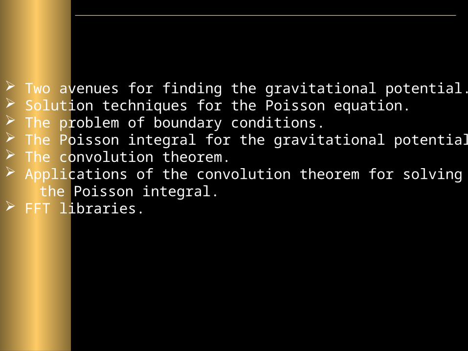
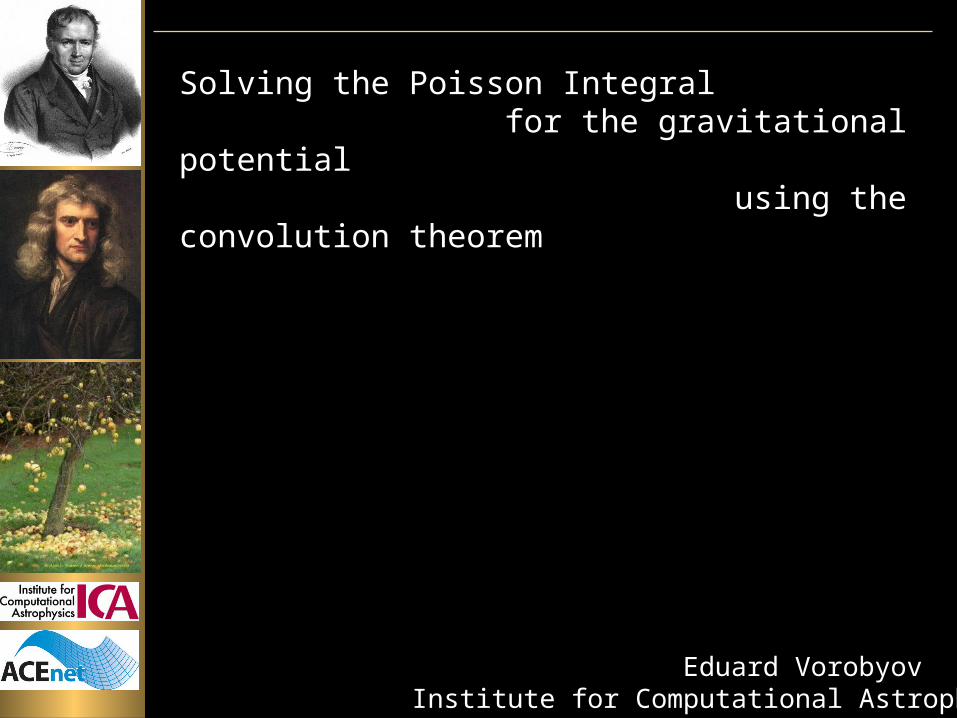
Two avenues for finding the gravitational potential. Solution techniques for the Poisson equation. The problem of boundary conditions. The Poisson integral for the gravitational potential. The convolution theorem. Applications of the convolution theorem for solving the Poisson integral. FFT libraries.

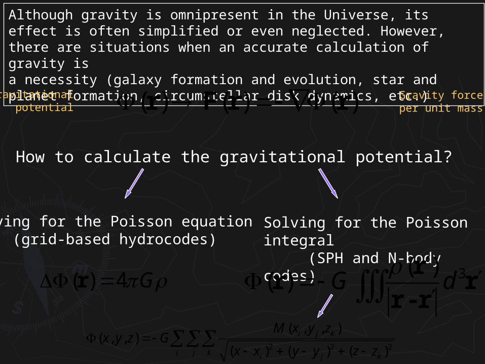
How to calculate the gravitational potential?

Although gravity is omnipresent in the Universe, its effect is often simplified or even neglected. However, there are situations when an accurate calculation of gravity is a necessity (galaxy formation and evolution, star and planet formation, circumstellar disk dynamics, etc.)

( ) ( ) ( ) r F r r

( ) 4 G r

Gravitational potential

Gravity forceper unit mass

Solving for the Poisson equation (grid-based hydrocodes)

Solving for the Poisson integral (SPH and N-body codes)

3( )( ) G d

r

r rr - r

2 2 2

( , , )( , , )

( ) ( ) ( )

i j k

i j k i j k

M x y zx y z G

x x y y z z

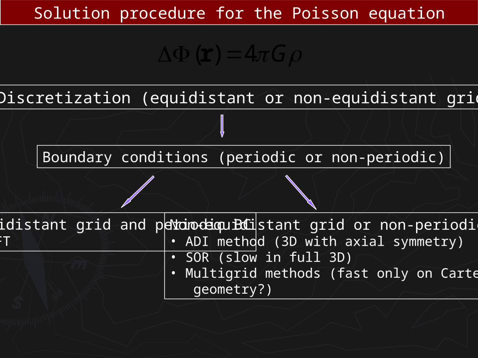
( ) 4 G r

Discretization (equidistant or non-equidistant grid)

Equidistant grid and periodic BC• FFT

Non-equidistant grid or non-periodic BC• ADI method (3D with axial symmetry)• SOR (slow in full 3D)• Multigrid methods (fast only on Cartesian geometry?)

Solution procedure for the Poisson equation

Boundary conditions (periodic or non-periodic)

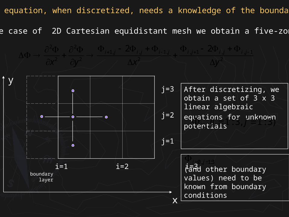
The Poisson equation, when discretized, needs a knowledge of the boundary values!

2 21, , 1, , 1 , , 1

2 2 2 2

2 2i j i j i j i j i j i j

x y x y

For a simple case of 2D Cartesian equidistant mesh we obtain a five-zone molecule

i=0 i=1 i=2 i=3

j=3

j=2

j=1

boundary layer

x

y

0, 1:3i j (and other boundary values) need to be known from boundary conditions

After discretizing, we obtain a set of 3 x 3 linear algebraic equations

for unknown potentials

, ( 1 : 3, 1 : 3)i j i j

i=0 i=1 i=2 i=3

j=3

j=2

j=1

boundary layer

x

y

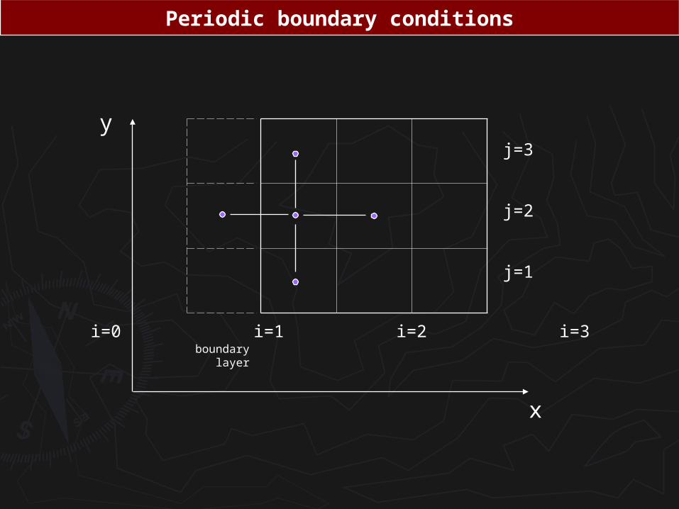
Periodic boundary conditions

i=0 i=1 i=2 i=3

j=3

j=2

j=1

boundary layer

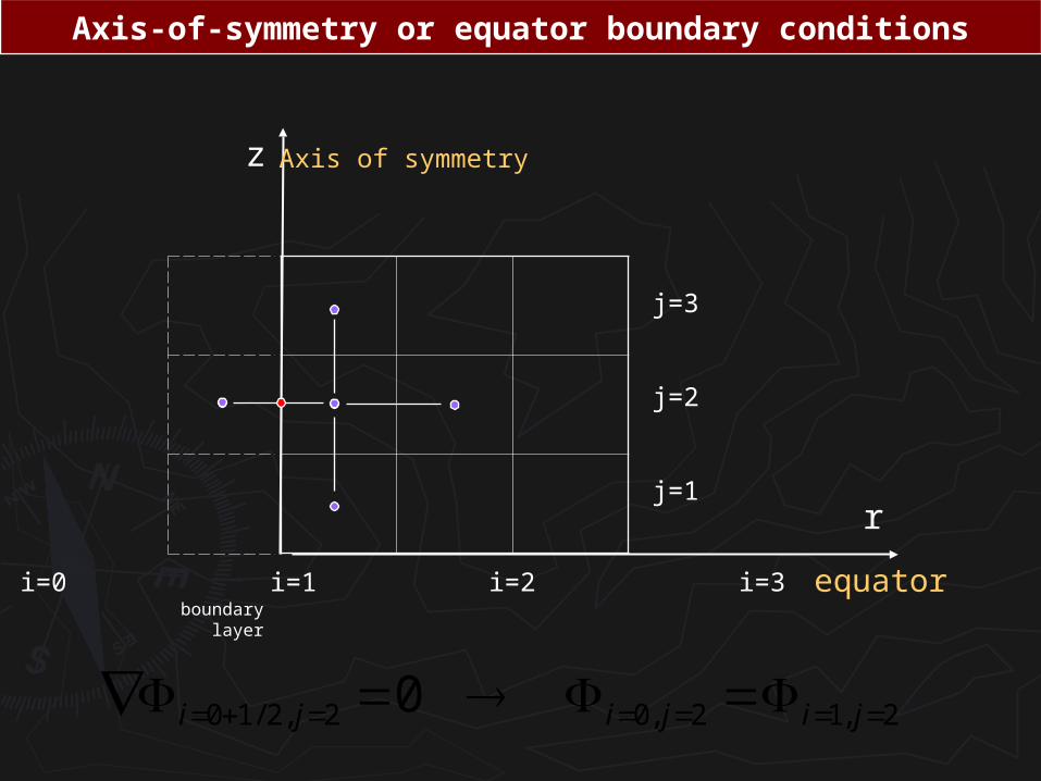
r

z

Axis-of-symmetry or equator boundary conditions

Axis of symmetry

0 1/ 2, 2 0, 2 1, 20i j i j i j

equator

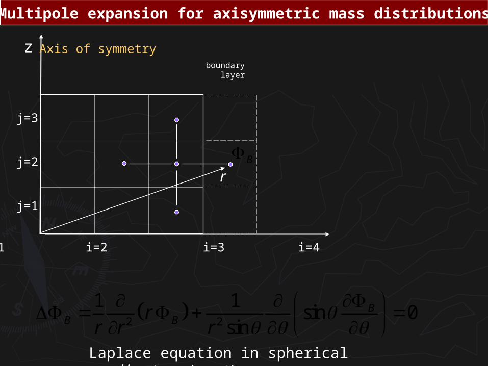
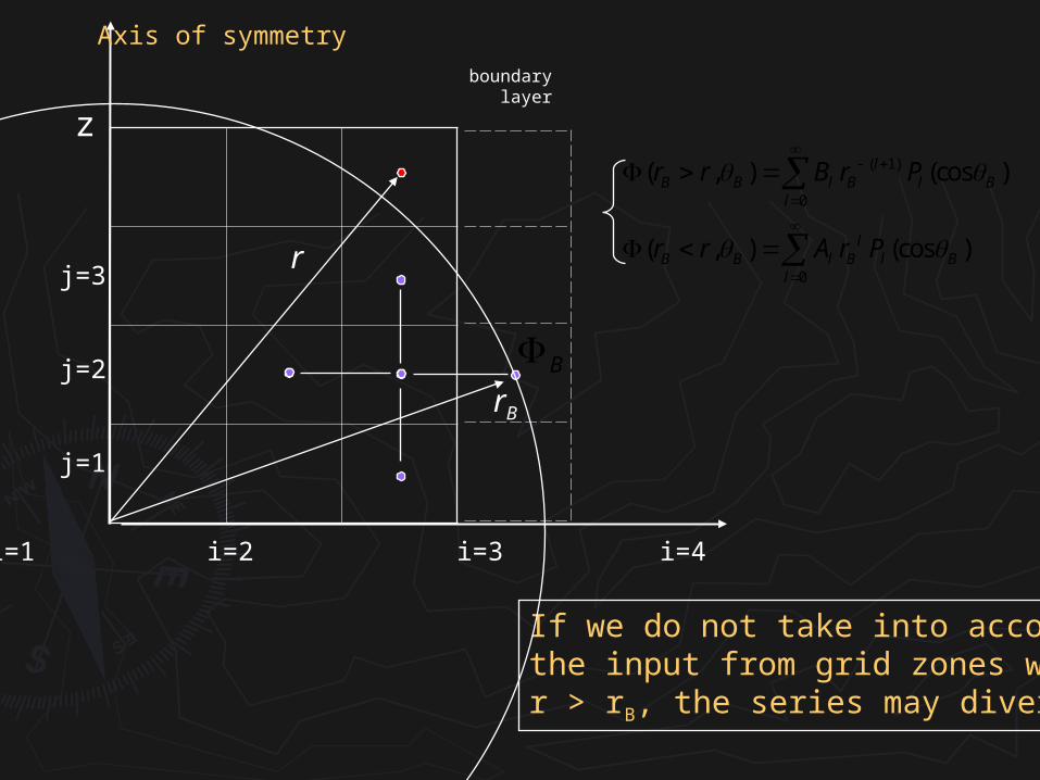
Multipole expansion for axisymmetric mass distributions

2 2

1 1sin 0

sinB

B Brr r r

i=1 i=2 i=3 i=4

j=3

j=2

j=1

boundary layer

z Axis of symmetry

Laplace equation in spherical coordinates (r,

rB

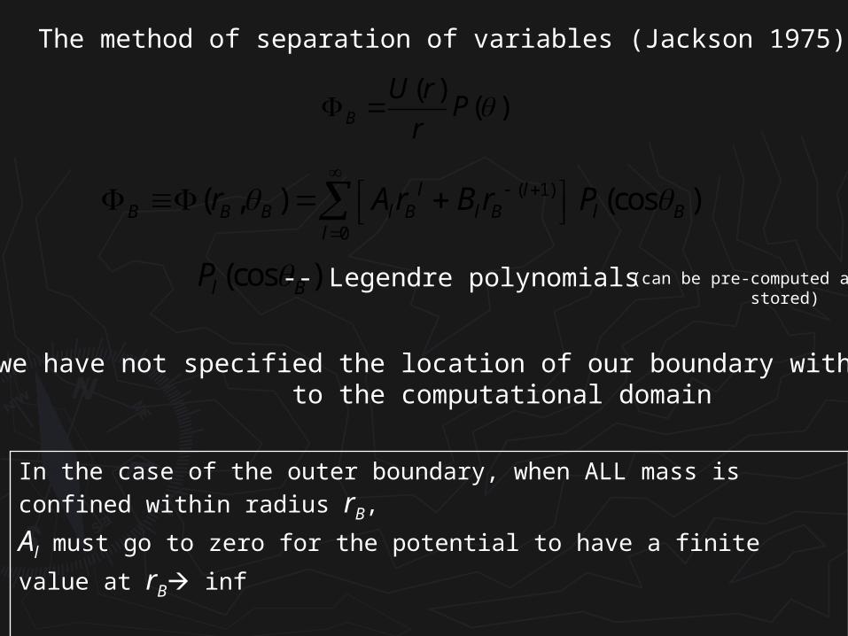
The method of separation of variables (Jackson 1975)

( )( )B

U rP

r

( 1)

0

( , ) (cos )l lB B B l B l B l B

l

r A r B r P

(cos )l BP -- Legendre polynomials

So far, we have not specified the location of our boundary with respect to the computational domain

In the case of the outer boundary, when ALL mass is confined within radius rB,

Al must go to zero for the potential to have a finite value at rB inf

In the opposite case of the inner boundary, Bl = 0.

(can be pre-computed and stored)

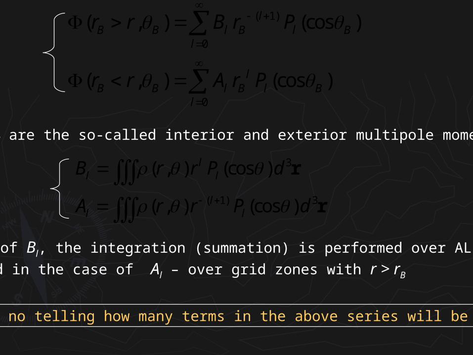
( 1)

0

0

( , ) (cos )

( , ) (cos )

lB B l B l B

l

lB B l B l B

l

r r B r P

r r A r P

Bl and Al are the so-called interior and exterior multipole moments

3

( 1) 3

( , ) (cos )

( , ) (cos )

ll l

ll l

B r r P d

A r r P d

r

r

In the case of Bl, the integration (summation) is performed over ALL grid zones

with r < rB and in the case of Al – over grid zones with r > rB

There is no telling how many terms in the above series will be needed!

i=1 i=2 i=3 i=4

j=3

j=2

j=1

boundary layer

z

Axis of symmetry

rB

B

( 1)

0

0

( , ) (cos )

( , ) (cos )

lB B l B l B

l

lB B l B l B

l

r r B r P

r r A r P

If we do not take into accountthe input from grid zones withr > rB, the series may diverge!

r

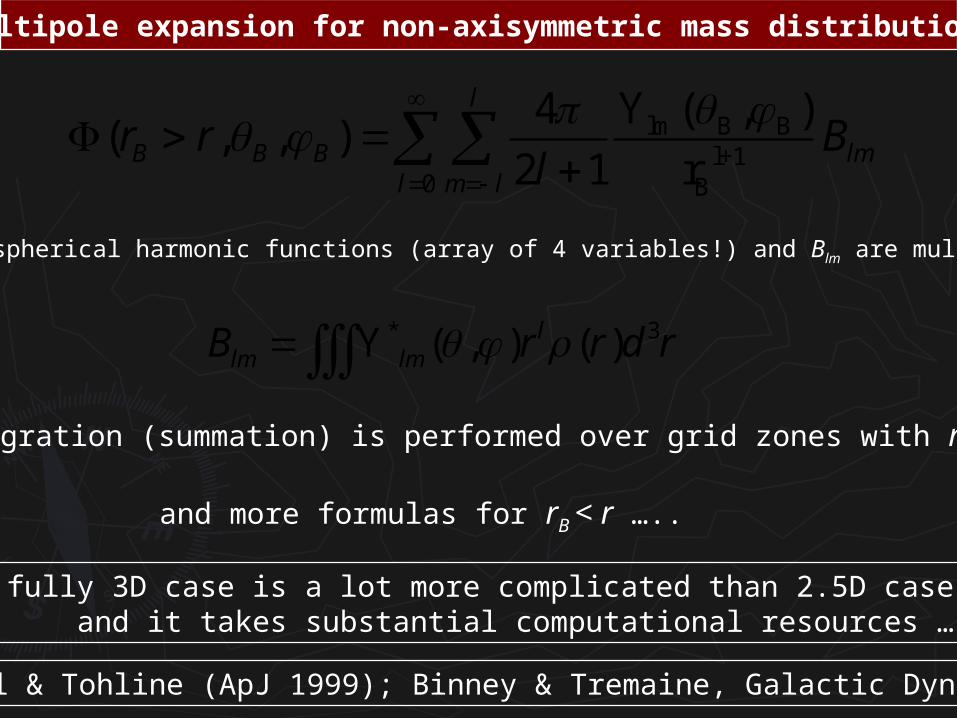
Multipole expansion for non-axisymmetric mass distributions

lm B Bl+1

0 B

4 Y ( , )( , , )

2 1 r

l

B B B lml m l

r r Bl

Ylm are the spherical harmonic functions (array of 4 variables!) and Blm are multipole moments

* 3Y ( , ) ( )llm lmB r r d r

The integration (summation) is performed over grid zones with r < rB

and more formulas for rB < r …..

The fully 3D case is a lot more complicated than 2.5D case and it takes substantial computational resources ….

See Cohl & Tohline (ApJ 1999); Binney & Tremaine, Galactic Dynamics

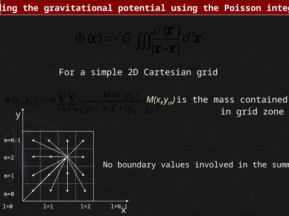
Finding the gravitational potential using the Poisson integral

3( )( ) G d

r

r rr - r

1 1

2 20 0

( , )( , )

( ) ( )

N Nl m

l ml m l l m m

M x yx y G

x x y y

For a simple 2D Cartesian grid

M(xl,ym) is the mass contained in grid zone (l,m)

x

y

l=0 l=1 l=2 l=N-1

m=N-1

m=2

m=1

m=0

No boundary values involved in the summation!

1 1 1 1

, ,2 2 2 20 0 0 0( ) ( )

N N N Nl m

l m l l m m l ml m l m

MG G M

x l l y m m

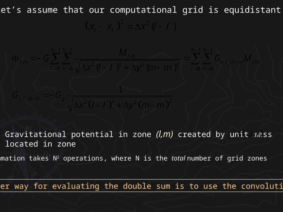
Now let’s assume that our computational grid is equidistant.

2 2( )l lx x x l l

, 2 22 2

1l l m m gG G

x l l y m m

Gravitational potential in zone (l,m) created by unit mass located in zone ,l m

A much faster way for evaluating the double sum is to use the convolution theorem

Direct summation takes N2 operations, where N is the total number of grid zones

1 1

, , ,'

A B CN N

l m l m l l m ml N m N

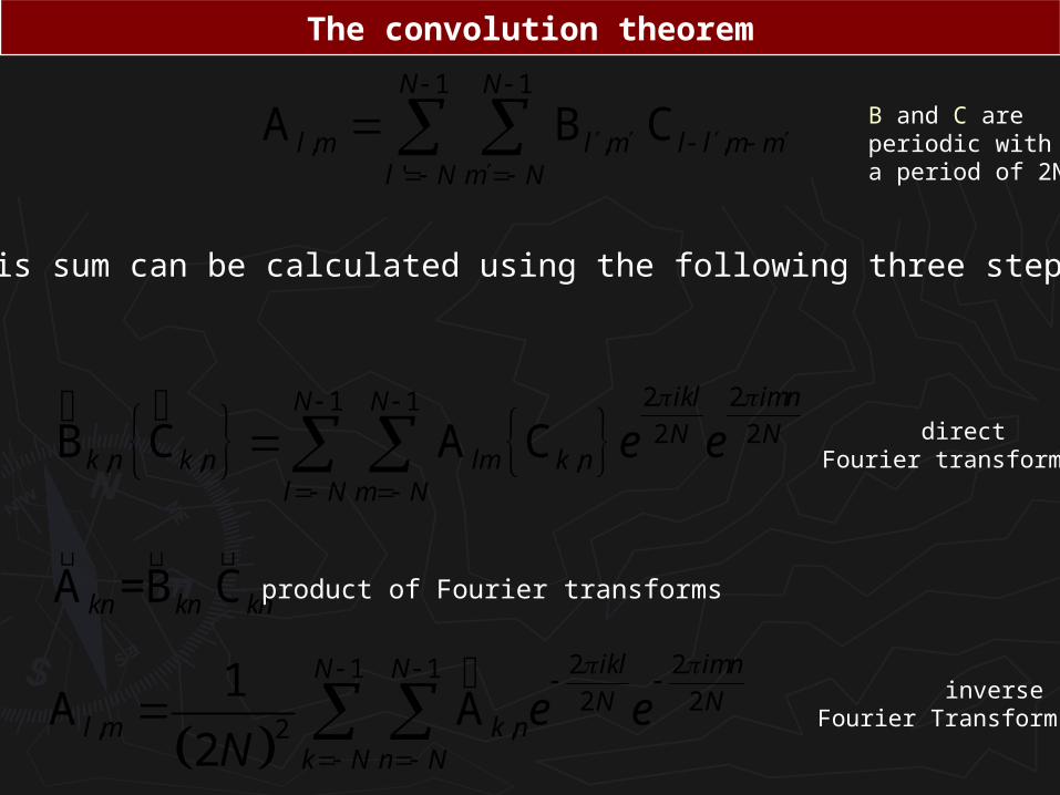
The convolution theorem

A =B Ckn kn kn

2 21 12 2

, , ,B C A Cikl imnN NN N

k n k n lm k nl N m N

e e

product of Fourier transforms

2 21 12 2

, ,2

1A A

2

ikl imnN NN N

l m k nk N n N

e eN

directFourier transform

inverseFourier Transform

This sum can be calculated using the following three steps

B and C areperiodic witha period of 2N

1 1

, , ,'

A B CN N

l m l m l l m ml N m N

1 1

, ,0 0

MN N

l m l m l l m ml m

G

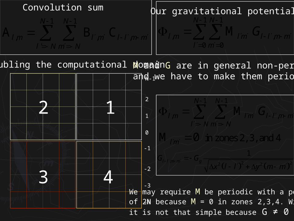
Doubling the computational domain

Convolution sum Our gravitational potential

N-1

2

1

0

-1

-2

-3

-N

12

3 4

M and G are in general non-periodicand we have to make them periodic

1 1

, ,

in zones 2, 3, and 4

M

M 0

N N

l m l m l l m ml N m N

l m

G

, 2 22 2

1l l m m gG G

x l l y m m

We may require M be periodic with a period of 2N because M = 0 in zones 2,3,4. With G

it is not that simple because G ≠ 0

N-1

2

1

0

-1

-2

-3

-N

12

3 4

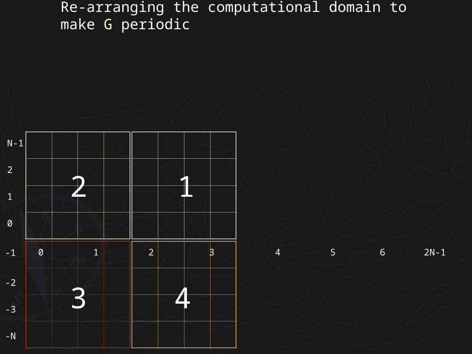
Re-arranging the computational domain to make G periodic

0 1 2 3 4 5 6 2N-1

12

3 4

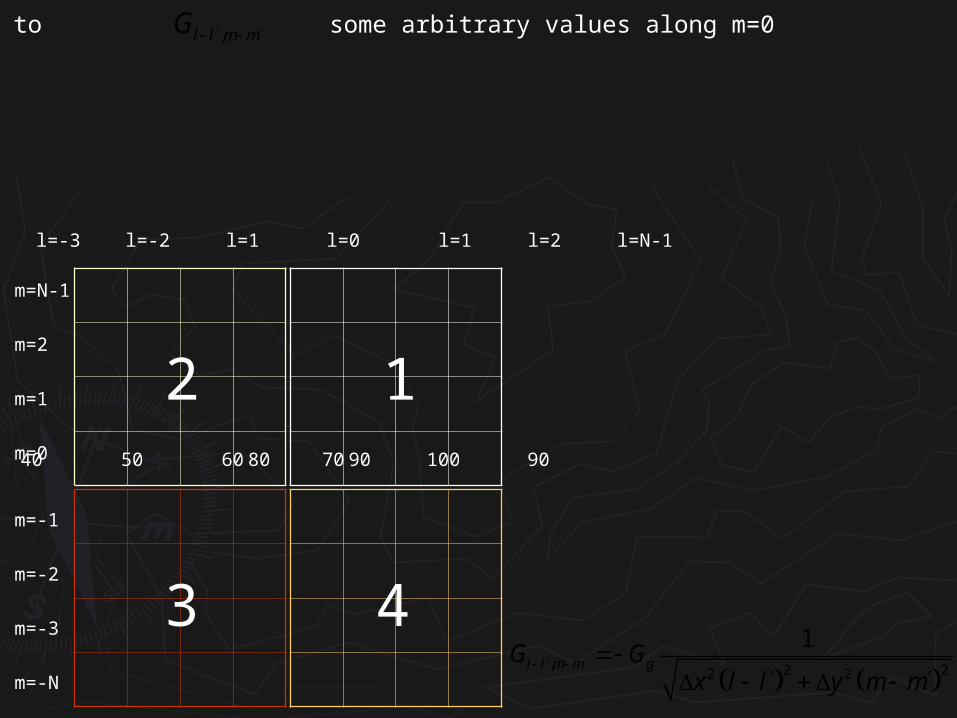
40 50 60 70 80 90 100 90

Let’s assign to some arbitrary values along m=0,l l m mG

, 2 22 2

1l l m m gG G

x l l y m m

l=-N l=-3 l=-2 l=1 l=0 l=1 l=2 l=N-1

m=N-1

m=2

m=1

m=0

m=-1

m=-2

m=-3

m=-N

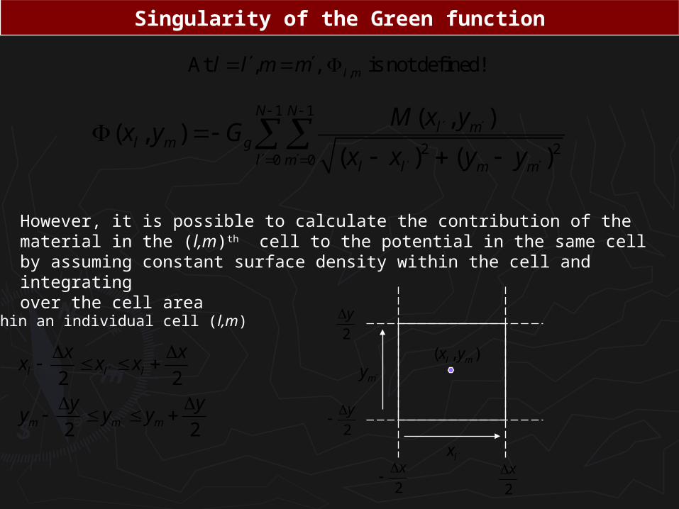
Singularity of the Green function

,At , , is not defined!l ml l m m

However, it is possible to calculate the contribution of the material in the (l,m)th cell to the potential in the same cell by assuming constant surface density within the cell and integratingover the cell area

1 1

2 20 0

( , )( , )

( ) ( )

N Nl m

l m gl m l l m m

M x yx y G

x x y y

2

x

2

y

2 2

2 2

l l l

m m m

x xx x x

y yy y y

within an individual cell (l,m)

2

x

2

y

lx

my

( , )l mx y

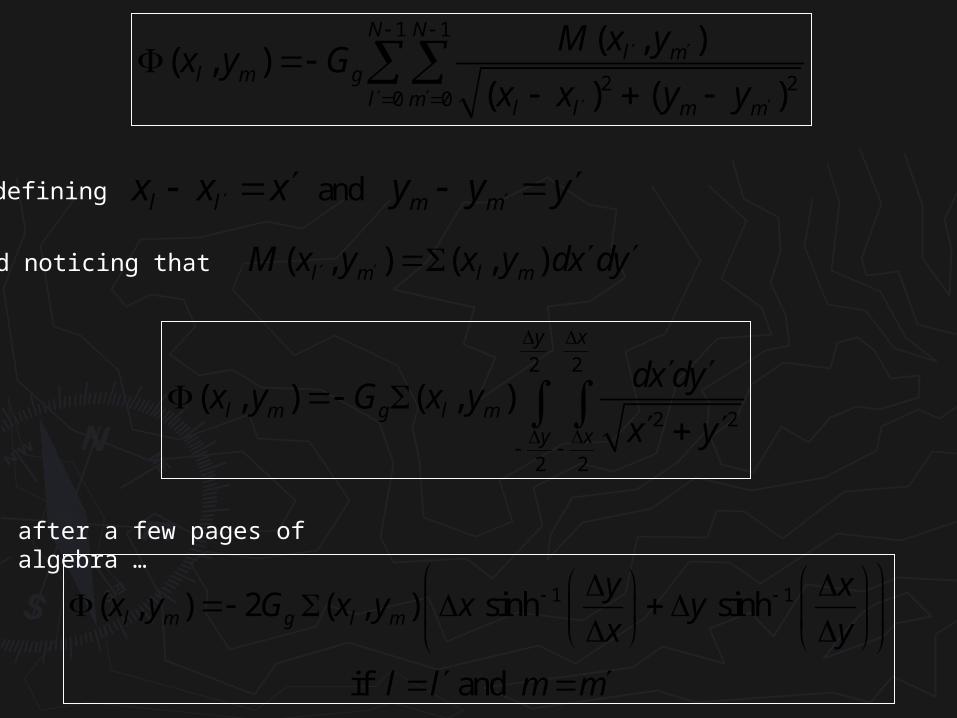
after a few pages of algebra …

1 1( , ) 2 ( , ) sinh sinh

if and

l m g l m

y xx y G x y x y

x y

l l m m

2 2

2 2

2 2

( , ) ( , )

y x

l m g l my x

dx dyx y G x y

x y

and l l m mx x x y y y defining

( , ) ( , )l m l mM x y x y dx dy and noticing that

1 1

2 20 0

( , )( , )

( ) ( )

N Nl m

l m gl m l l m m

M x yx y G

x x y y

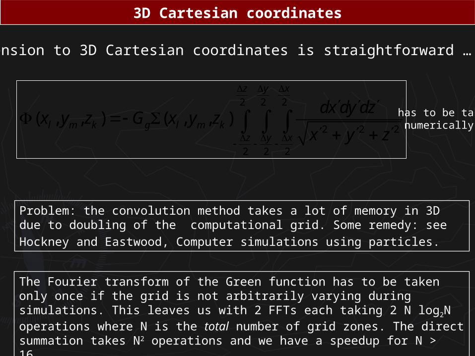
3D Cartesian coordinates

The extension to 3D Cartesian coordinates is straightforward …

2 2 2

2 2 2

2 2 2

( , , ) ( , , )

z y x

l m k g l m kz y x

dx dy dzx y z G x y z

x y z

has to be taken numerically ….

Problem: the convolution method takes a lot of memory in 3D due to doubling of the computational grid. Some remedy: see Hockney and Eastwood, Computer simulations using

particles.

The Fourier transform of the Green function has to be taken only once if the grid is not arbitrarily varying during simulations. This leaves us with 2 FFTs each taking 2 N log2N operations where N is the total number of grid zones. The direct summation takes N2 operations and we have a speedup for N > 16.

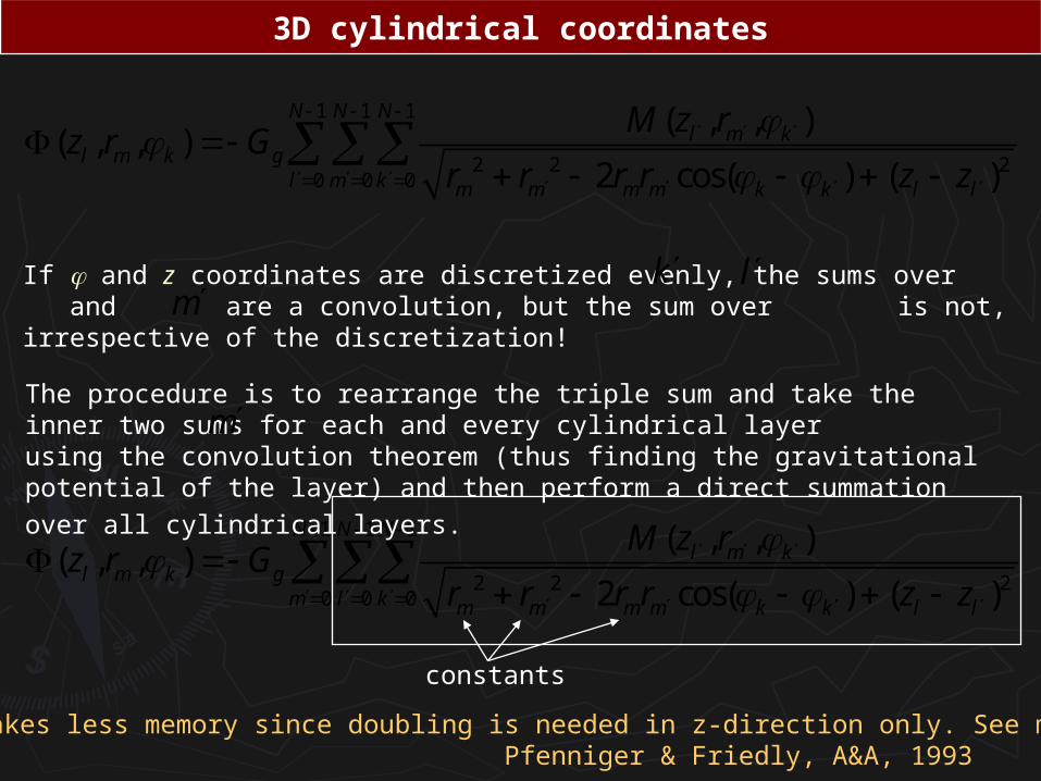
3D cylindrical coordinates

1 1 1

2 2 20 0 0

( , , )( , , )

2 cos( ) ( )

N N Nl m k

l m k gl m k m m m m k k l l

M z rz r G

r r r r z z

If and z coordinates are discretized evenly, the sums over and are a convolution, but the sum over is not, irrespective of the discretization!

k lm

1 1 1

2 2 20 0 0

( , , )( , , )

2 cos( ) ( )

N N Nl m k

l m k gm l k m m m m k k l l

M z rz r G

r r r r z z

The procedure is to rearrange the triple sum and take the inner two sums for each and every cylindrical layer using the convolution theorem (thus finding the gravitational potential of

the layer) and then perform a direct summation over all cylindrical layers. m

constants

Slower, but takes less memory since doubling is needed in z-direction only. See more details in Pfenniger & Friedly, A&A, 1993

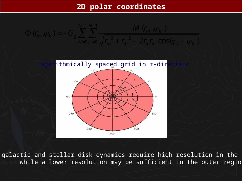
2D polar coordinates

1 1

2 20 0

( , )( , )

2 cos( )

N Nm k

m k gm k m m m m k k

M rr G

r r r r

Logarithmically spaced grid in r-direction

Simulations of galactic and stellar disk dynamics require high resolution in the inner regions, while a lower resolution may be sufficient in the outer regions

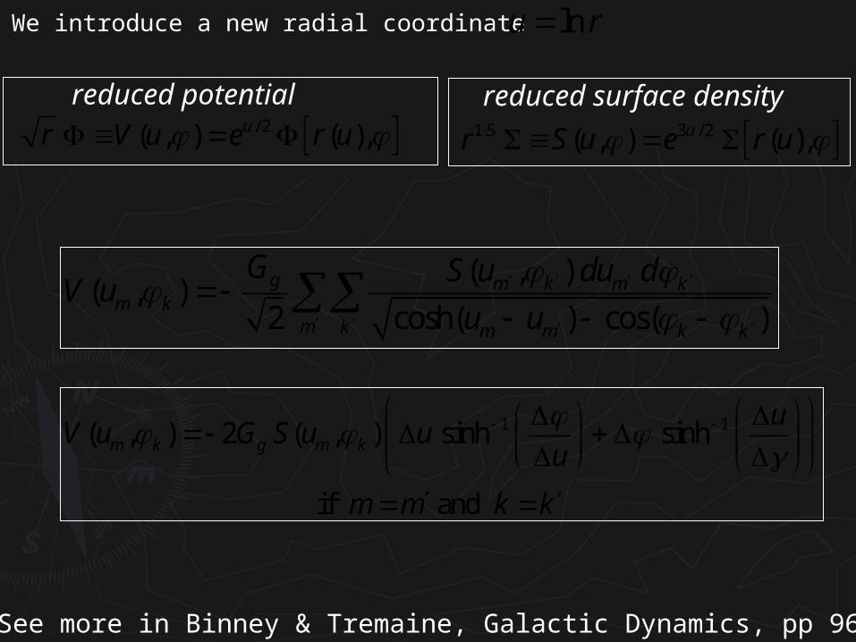
/ 2( , ) ( ),ur V u e r u reduced potential

We introduce a new radial coordinate lnu r

reduced surface density

1.5 3 / 2( , ) ( ),ur S u e r u

( , )( , )

2 cosh( ) cos( )g m k m k

m km k m m k k

G S u du dV u

u u

1 1( , ) 2 ( , ) sinh sinh

if and

m k g m k

uV u G S u u

u

m m k k

See more in Binney & Tremaine, Galactic Dynamics, pp 96-97.

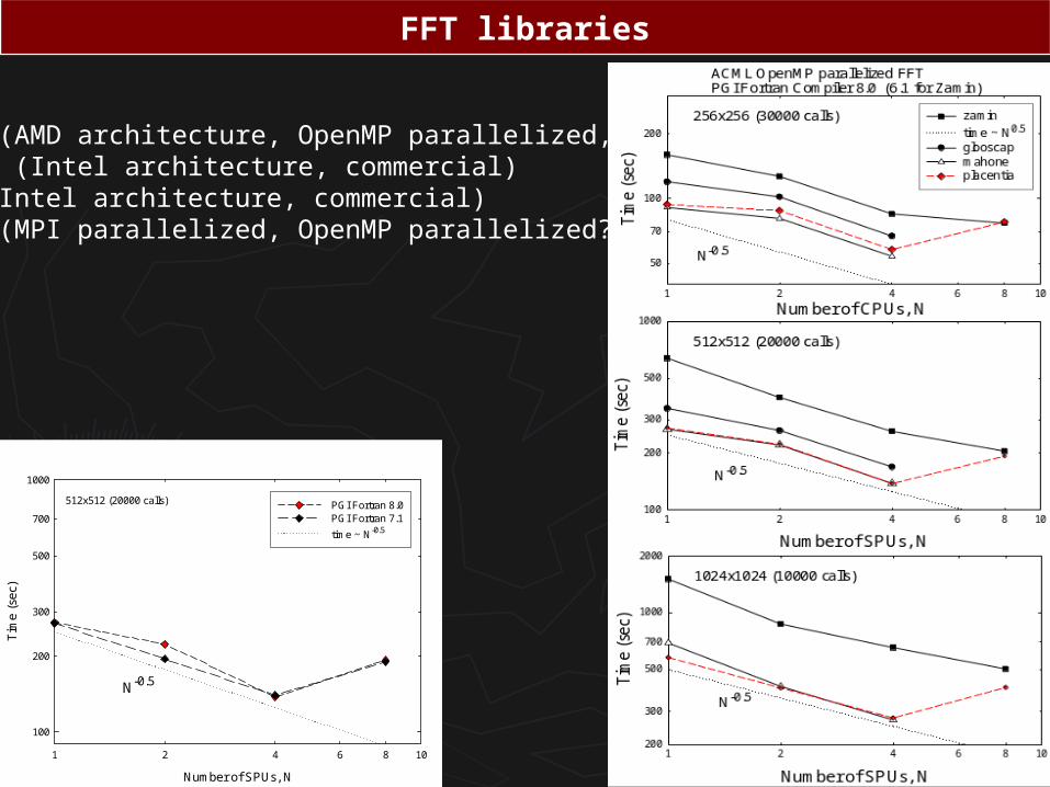
FFT libraries

• ACML (AMD architecture, OpenMP parallelized, free)• ICML (Intel architecture, commercial) • MKL (Intel architecture, commercial)• FFTW (MPI parallelized, OpenMP parallelized?, free)

Number of SPUs, N

2 4 6 81 10

Tim

e (

sec)

200

300

500

700

100

1000

PGI Fortran 8.0PGI Fortran 7.1

time ~ N-0.5

N-0.5

512x512 (20000 calls)

Thank you!