Solving the Heat Equation with the Quadrupole Approach

P.Y. Sulima, J.L. Battaglia, T. ZimmerUniversity Bordeaux 1

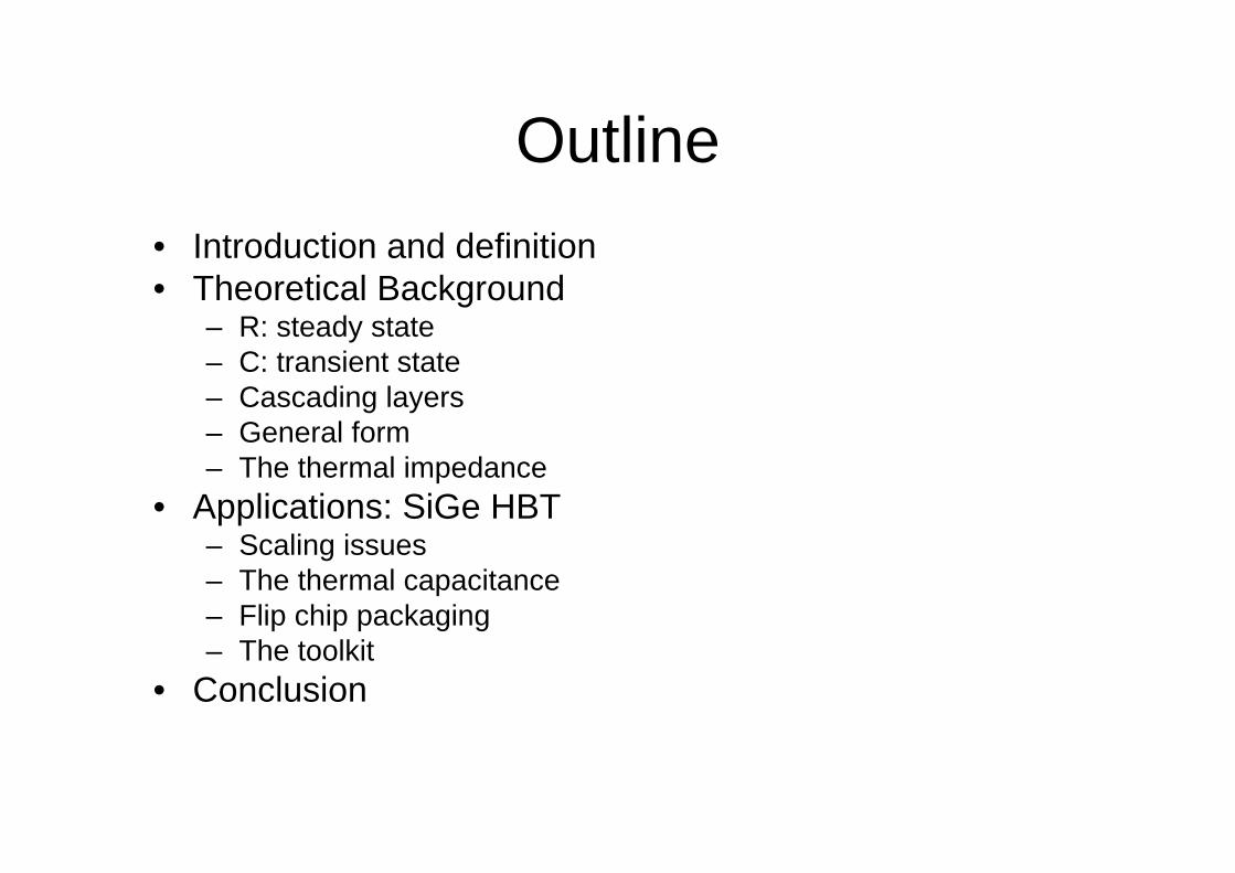
Outline• Introduction and definition• Theoretical Background

– R: steady state– C: transient state– Cascading layers– General form– The thermal impedance

• Applications: SiGe HBT– Scaling issues– The thermal capacitance– Flip chip packaging– The toolkit

• Conclusion

Modeling of diffusive heat transfer, SOA

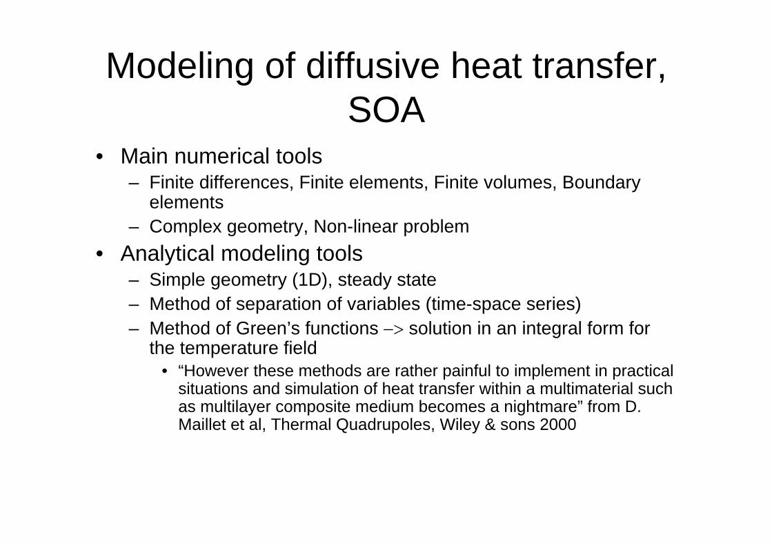
• Main numerical tools– Finite differences, Finite elements, Finite volumes, Boundary

elements– Complex geometry, Non-linear problem

• Analytical modeling tools– Simple geometry (1D), steady state– Method of separation of variables (time-space series)– Method of Green’s functions −> solution in an integral form for

the temperature field• “However these methods are rather painful to implement in practical

situations and simulation of heat transfer within a multimaterial such as multilayer composite medium becomes a nightmare” from D. Maillet et al, Thermal Quadrupoles, Wiley & sons 2000

Modeling of diffusive heat transfer, Quadrupole method

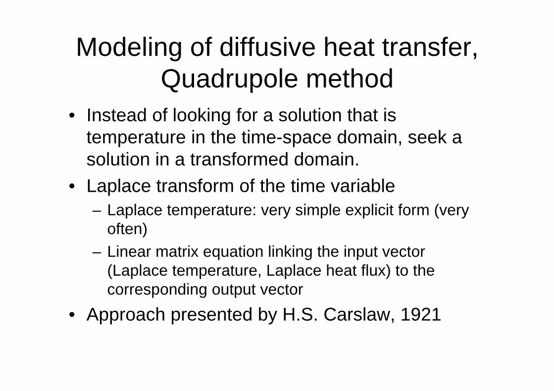
• Instead of looking for a solution that is temperature in the time-space domain, seek a solution in a transformed domain.

• Laplace transform of the time variable – Laplace temperature: very simple explicit form (very

often)– Linear matrix equation linking the input vector

(Laplace temperature, Laplace heat flux) to the corresponding output vector

• Approach presented by H.S. Carslaw, 1921

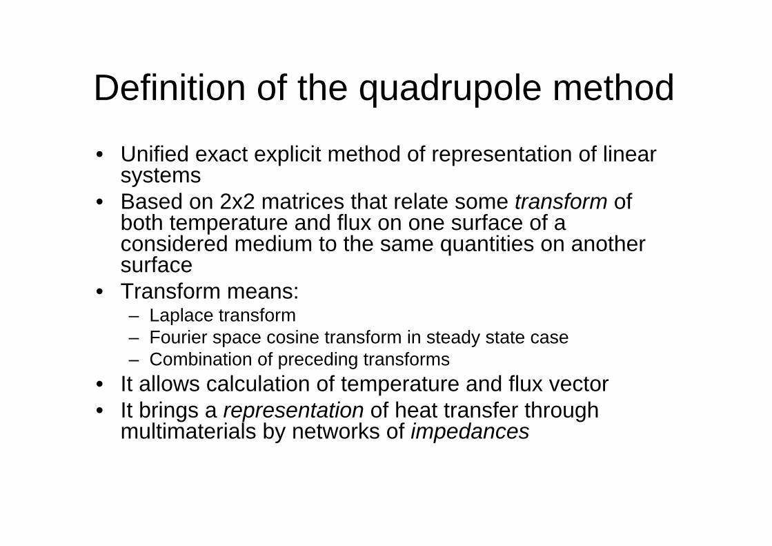
Definition of the quadrupole method

• Unified exact explicit method of representation of linear systems

• Based on 2x2 matrices that relate some transform of both temperature and flux on one surface of a considered medium to the same quantities on another surface

• Transform means:– Laplace transform– Fourier space cosine transform in steady state case– Combination of preceding transforms

• It allows calculation of temperature and flux vector• It brings a representation of heat transfer through

multimaterials by networks of impedances

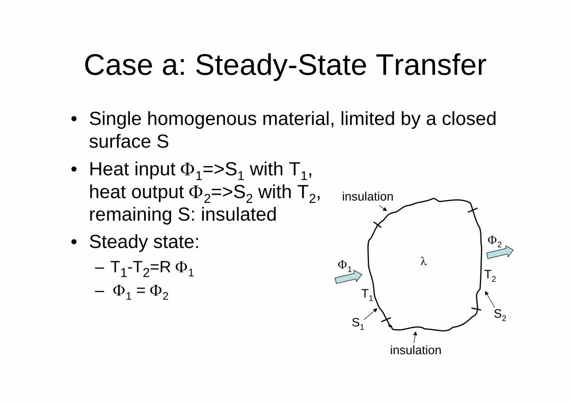
Case a: Steady-State Transfer

• Single homogenous material, limited by a closed surface S

• Heat input Φ1=>S1 with T1,heat output Φ2=>S2 with T2, remaining S: insulated

• Steady state:– T1-T2=R Φ1

– Φ1 = Φ2

λ

Φ2

Φ1

S1

T1

T2

insulation

insulation

S2

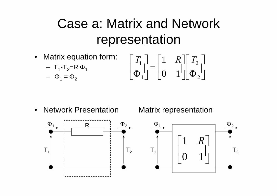
Case a: Matrix and Network representation

• Matrix equation form:– T1-T2=R Φ1

– Φ1 = Φ2

• Network Presentation Matrix representation

⎥⎦

⎤⎢⎣

⎡Φ⎥

⎦

⎤⎢⎣

⎡=⎥

⎦

⎤⎢⎣

⎡Φ 2

2

1

1

101 TRT

T1 T2

Φ1 Φ2R

T1 T2

Φ1 Φ2

⎥⎦

⎤⎢⎣

⎡10

1 R

Case b: Transient-State• Same system as before,

but transient conditions• At t=0, T uniform,

Heat input Φ1=>S1heat output Φ2=>S2remaining S: insulated

• conductivity λ is large enough to assume, that T(t) is uniform

• Heat balance:

– Mass density: ρ, Specific heat: c, Volume: V, Heat capacity: Ct=ρcV

( ) ( )tttdTdVc 21 Φ−Φ=ρ

S2

ρ, c, V

Φ2

Φ1

S1

T1

T2

insulation

insulation

T(t)

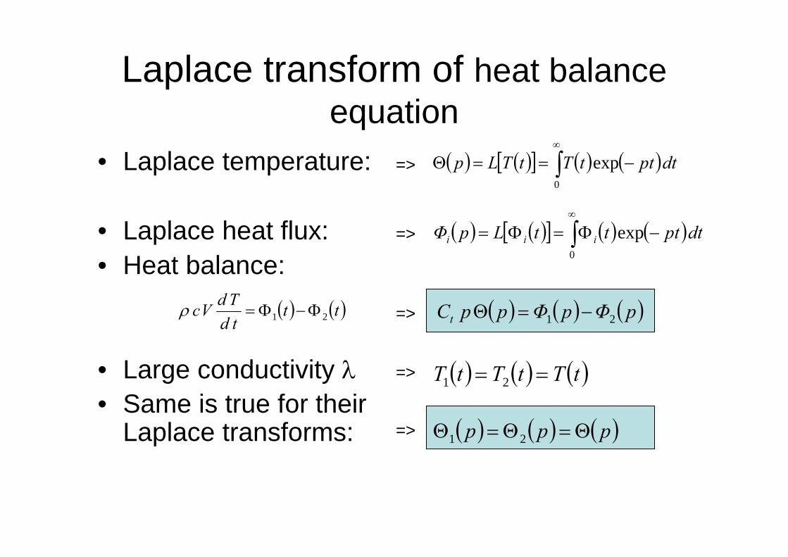
Laplace transform of heat balance equation

• Laplace temperature:

• Laplace heat flux:• Heat balance:

• Large conductivity λ• Same is true for their

Laplace transforms:

( ) ( )[ ] ( ) ( )dtpttTtTLp −==Θ ∫∞

exp0

( ) ( )[ ] ( ) ( )dtptttLpΦ iii −Φ=Φ= ∫∞

exp0

( ) ( )tttdTdVc 21 Φ−Φ=ρ ( ) ( ) ( )pΦpΦppCt 21 −=Θ=>

( ) ( ) ( )ppp Θ=Θ=Θ 21

( ) ( ) ( )tTtTtT == 21=>

=>

=>

=>

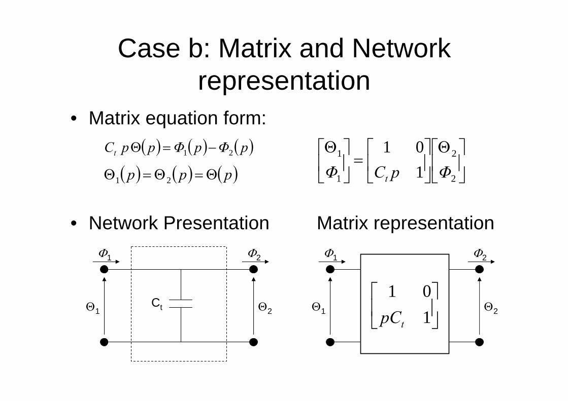
Case b: Matrix and Network representation

• Matrix equation form:

• Network Presentation Matrix representation

⎥⎦

⎤⎢⎣

⎡Θ⎥⎦

⎤⎢⎣

⎡=⎥

⎦

⎤⎢⎣

⎡Θ

2

2

1

1

101

ΦpCΦ t

Θ1 Θ2

Φ1 Φ2

⎥⎦

⎤⎢⎣

⎡101

tpCΘ1 Θ2

Φ1 Φ2

Ct

( ) ( ) ( )pΦpΦppCt 21 −=Θ

( ) ( ) ( )ppp Θ=Θ=Θ 21

Case c: Cascading layers

• Cascade of two media

– Steady state:

– Transient state:

⎥⎦

⎤⎢⎣

⎡Φ⎥

⎦

⎤⎢⎣

⎡ +=⎥

⎦

⎤⎢⎣

⎡Φ⎥

⎦

⎤⎢⎣

⎡⎥⎦

⎤⎢⎣

⎡=⎥

⎦

⎤⎢⎣

⎡Φ 2

221

2

221

1

1

101

101

101 TRRTRRT

( ) ⎥⎦

⎤⎢⎣

⎡Θ⎥⎦

⎤⎢⎣

⎡+

=⎥⎦

⎤⎢⎣

⎡Θ⎥⎦

⎤⎢⎣

⎡⎥⎦

⎤⎢⎣

⎡=⎥

⎦

⎤⎢⎣

⎡Θ

2

2

212

2

11

1

101

1201

101

ΦpCCΦpCpCΦ tttt

T1 T2

Φ1 Φ2R1+R2

Θ1 Θ2

Φ1 Φ2

Ct1+Ct2

S2

Φ2Φ1

S1

T1T2

(2)Φi

Ti

(1)

Si

Limitations

• Steady state: – average surface T (no local T), – external representation

• Transient state: – strong assumption of uniform temperature distribution– no geometrical data are used to calculate Ct (zero-

dimensional model)• Question: how it is possible to extend and

combine steady state and transient state models?

Case d: an infinite layer• Things simplify a lot …

– Layer with thickness e,– thermal conductivity λ, – volumetric heat capacity ρc, – mass density ρ, specific heat c, – thermal diffusivity a = λ / ρc, – cross section S

• 1-D Heat transfer: temperature field T(x,t)

• Heat flux Φ at any location x inside the layer:

0102

2

==∂∂

=∂∂ tforTTwith

tT

axT

xTS

∂∂

−=Φ λ

Φ1 Φ2

x

T1 T2

S

a=λ/ρce0

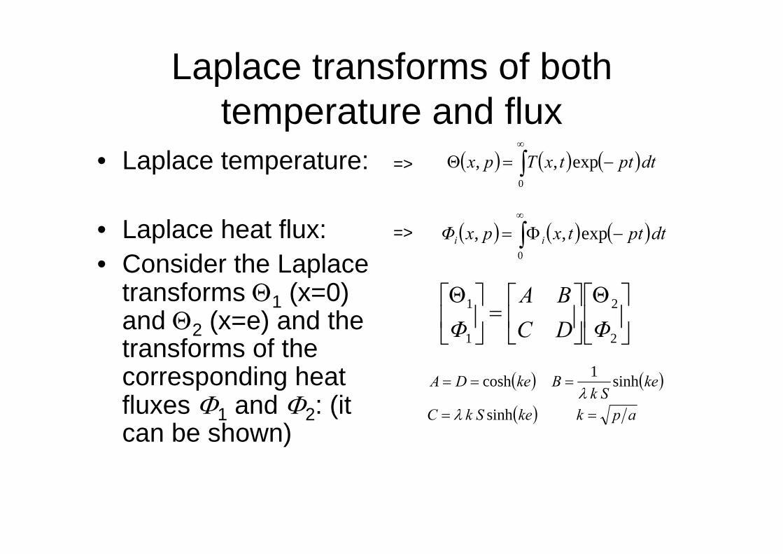
Laplace transforms of both temperature and flux

• Laplace temperature:

• Laplace heat flux:• Consider the Laplace

transforms Θ1 (x=0) and Θ2 (x=e) and the transforms of the corresponding heat fluxes Φ1 and Φ2: (it can be shown)

⎥⎦

⎤⎢⎣

⎡Θ⎥⎦

⎤⎢⎣

⎡=⎥

⎦

⎤⎢⎣

⎡Θ

2

2

1

1

ΦDCBA

Φ

( ) ( ) ( )dtpttxTpx −=Θ ∫∞

exp,,0

( ) ( ) ( )dtpttxpxΦ ii −Φ= ∫∞

exp,,0

=>

=>

( ) ( )

( ) apkkeSkC

keSk

BkeDA

==

===

sinh

sinh1cosh

λλ

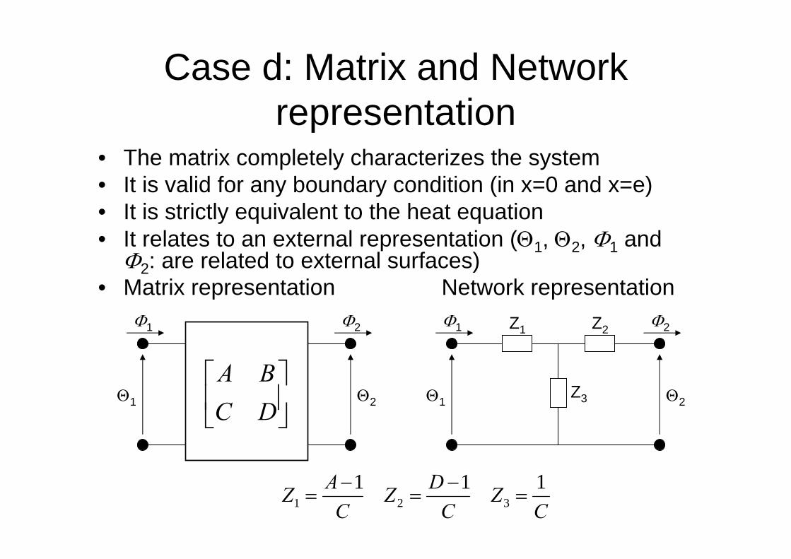
Case d: Matrix and Network representation

• The matrix completely characterizes the system• It is valid for any boundary condition (in x=0 and x=e)• It is strictly equivalent to the heat equation• It relates to an external representation (Θ1, Θ2, Φ1 and

Φ2: are related to external surfaces)• Matrix representation Network representation

Θ1 Θ2

Φ1 Φ2

⎥⎦

⎤⎢⎣

⎡DCBA

Θ1 Θ2

Φ1 Φ2

Z3

Z2Z1

CZ

CDZ

CAZ 111

321 =−

=−

=

Case d: heat pulse response• Assumption:

– the front face is excited by a Dirac heat pulse of energy Q

– The rear face remains insulated

• Translation into Laplace domain

• The system becomes:• Calculation (plotting) in

time domain– Inversion of the Laplace

transform (e.g. numerical with Stehfest’s algorithm

exxtQS

==Φ==Φ

at00at)(δ

exΦΦxΦQSΦ

======

at00at

2

1

221221 ΦDCΦΦBA +Θ=+Θ=Θ

( )( )apeap

QCAQS

apeapQ

CQS

tanh

sinh

1

2

λ

λ

==Θ

==Θ

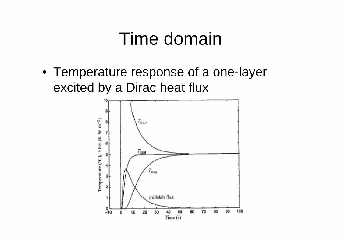
Time domain

• Temperature response of a one-layer excited by a Dirac heat flux

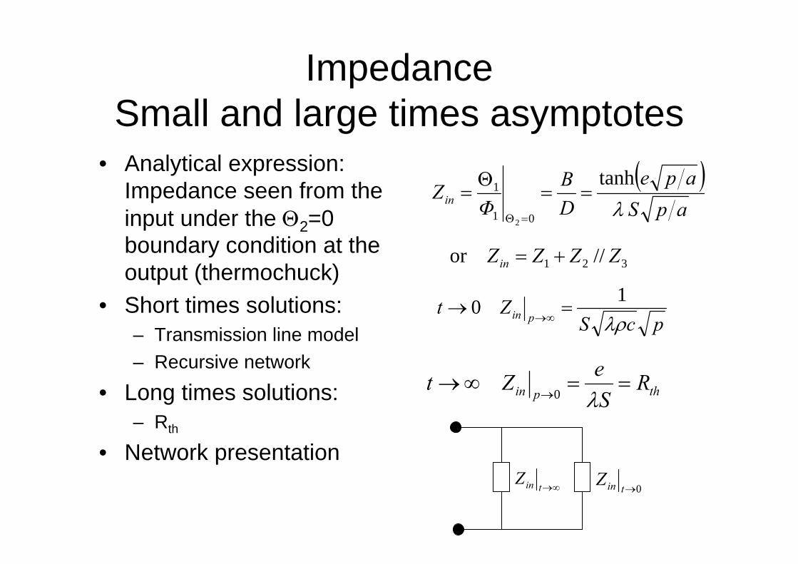
ImpedanceSmall and large times asymptotes

• Analytical expression: Impedance seen from the input under the Θ2=0 boundary condition at the output (thermochuck)

• Short times solutions:– Transmission line model– Recursive network

• Long times solutions:– Rth

• Network presentation

( )apSape

DB

ΦZin λ

tanh

01

1

2

==Θ

==Θ

pcSZt

pin λρ10 =→

∞→

thpin RSeZt ==∞→

→ λ0

321 //or ZZZZin +=

0→tinZ∞→tinZ

Application to Si/SiGe HBT

• Cross section:– 3 layers

• Back end• Insight deep trench

with heat source• substrate

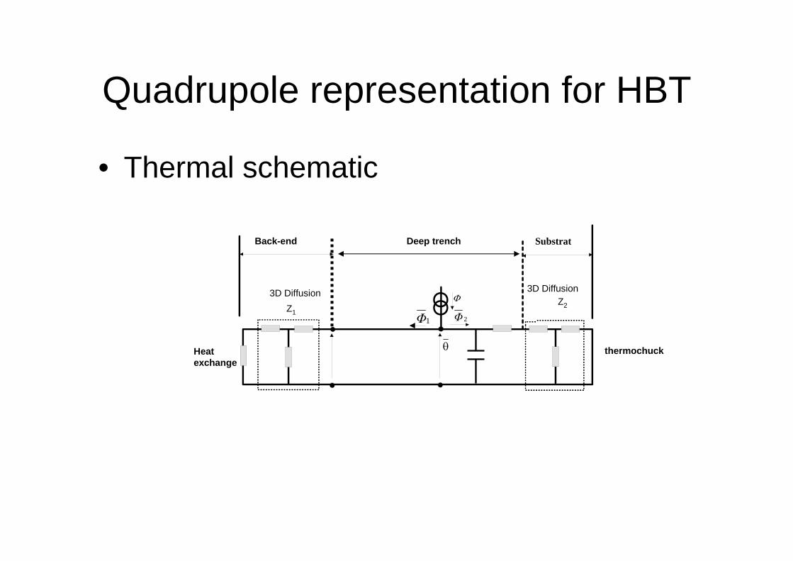
Quadrupole representation for HBT

• Thermal schematic

Substrat

2Φ1Φ

θ

Z1

Φ

Back-end

3D Diffusion 3D DiffusionZ2

Deep trench

Heat exchange

thermochuck

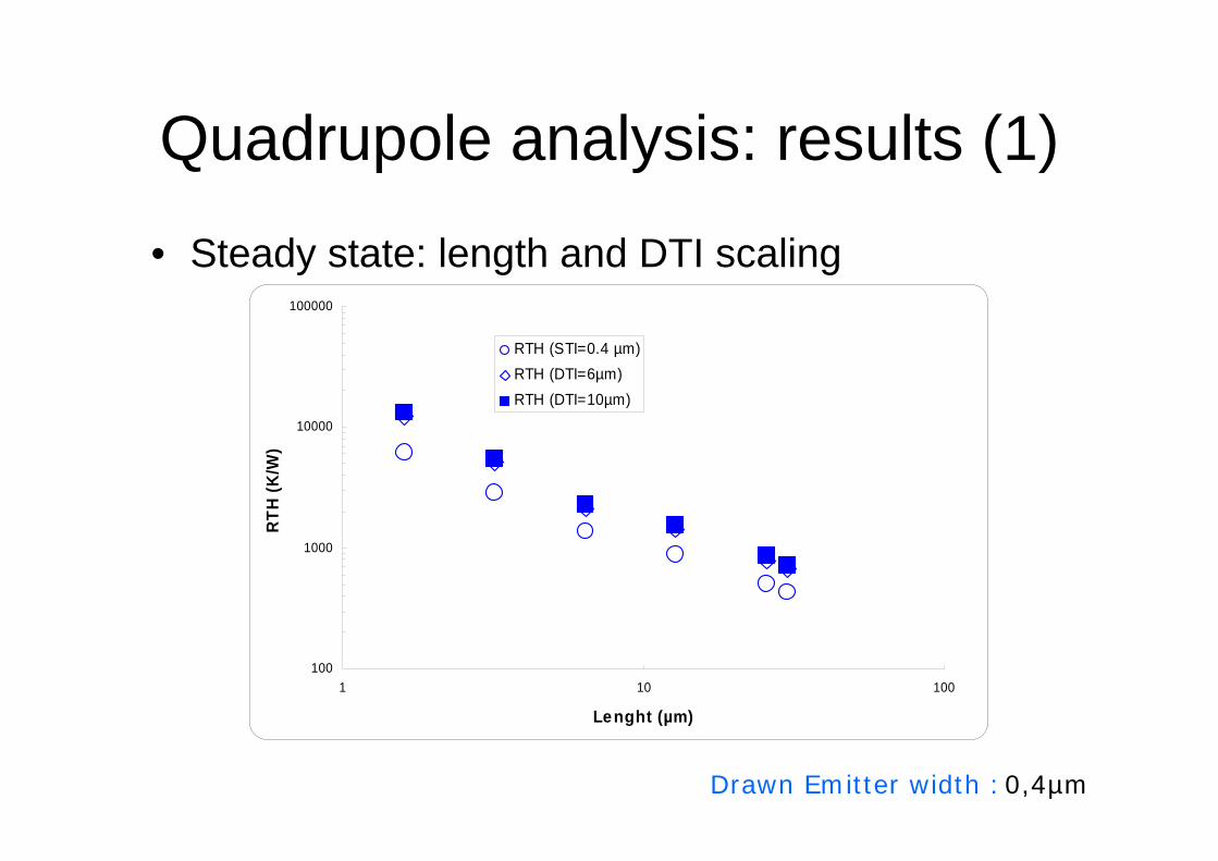
Quadrupole analysis: results (1)

• Steady state: length and DTI scaling

100

1000

10000

100000

1 10 100

Lenght (µm)

RTH

(K/W

)

RTH (STI=0.4 µm)RTH (DTI=6µm)RTH (DTI=10µm)

Drawn Emitter width :0,4µm

Quadrupole analysis: results (2)

• Transient state: length scaling

1.00E-12

1.00E-11

1.00E-10

1.00E-091 10 100

Lenght (µm)C

TH (J

/K)

CTH(STI)CTH(DTI=6µm)CTH(DTI=10µm)

Drawn Emitter width :0,4µm

Quadrupole analysis: results (3)

• Steady state: Emitter number and DTI scaling

0

200

400

600

800

1000

1200

1400

1600

1800

0 1 2 3 4 5 6 7 8 9

Emitte r number

RTH

(K/W

)

RTH(STI)RTH(DTI=6µm)RTH(DTI=10µm)

Drawn Emitter Surface : 30x0,4µm2

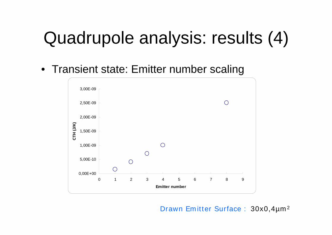
Quadrupole analysis: results (4)

• Transient state: Emitter number scaling

0,00E+00

5,00E-10

1,00E-09

1,50E-09

2,00E-09

2,50E-09

3,00E-09

0 1 2 3 4 5 6 7 8 9

Emitter number

CTH

(J/K

)

CTH(STI)CTH(DTI=6µm)CTH(DTI=10µm)

Drawn Emitter Surface : 30x0,4µm2

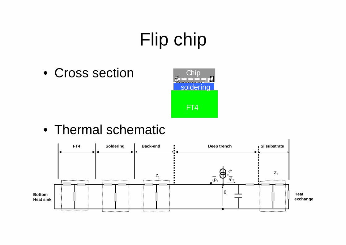
Flip chip

• Cross section

• Thermal schematic

Chip

soldering

FT4

2Φ1Φ

θ

Z1

Φ

Back-end

Z2

Deep trench

BottomHeat sink

Heatexchange

SolderingFT4 Si substrate

Flip chip: result

• Proof of concept

10-8 10-6 10-4 10-2 1000

2

4

6

8

10

12

14

16

18

Time (secondes)

Del

taT

(K)

Alone transistor thermogram (1)Flip chip transistor thermogram (2)Asymptotic curve (1)Asymptotic curve (2)

Chip

soldering

FT4

ToolkitIn one click…

Component description

Results

Discussion• Quadrupole network for heat exchange modeling• Analytical results: fast and accurate• External approach (no internal temperature field)• Thermal impedance• Well adapted for compact modeling• Extensible for specific configurations

– Multi-emitter fingers– Multi-cells (PA)– Mutual coupling (under work)– Packaging– Flip chip

• Versatile toolkit

One minute left• References

– Thermal quadrupoles, solving the heat equation through integrals transforms, D. Maillet, S. André, J.C. Batsale A. Degiovanni, C. Moyne, Ed. Wiley, 2000

– Pierre-Yvan Sulima, Contribution à la modélisation thermique des transistors bipolaires à hétérojonction SiGe, thesis, Université Bordeaux 1, defense : 13 décembre 2005

– Hassène Mnif, Contribution à la modélisation des transistors bipolaires àhétérojonction SiGe en température, thesis, Université Bordeaux 1, defense : 26 janvier 2004

– Helene Beckrich, Caractérisation, modélisation et conception de transistors RF de puissance intégrés dans une filières BiCMOS submicronique, thesis, Université Bordeaux 1, defense : 27 november 2006

– Yves Zimmermann, Modeling of spatially distributed and sizing effects in high-performance bipolar transistors, Master thesis, TU Dresden, June 2004,

• Acknowledgement– Thanks to the modeling and technology teams from ST Microelectronics for

device support and fruitful discussions– Nano2008, Minefi, Ministère de l’économie, des finances et de l’emploi (French

ministry of economy, finance and work)

END

• Thank you for your attention