SOLVING THE COURSE SCHEDULING PROBLEM BY CONSTRAINT PROGRAMMING AND

SIMULATED ANNEALING

A Thesis Submitted to the Graduate School of Engineering and Science of

İzmir Institute of Technology in Partial Fulfilment of the Requirements for the Degree of

MASTER OF SCIENCE

in Computer Software

by Esra AYCAN

November 2008 İZMİR

We approve the thesis of Esra AYCAN ______________________________

Asst. Prof. Dr. Tolga AYAV Supervisor ______________________________

Prof. Dr. Tatyana YAKHNO Committee Member ______________________________

Prof. Dr. Halis PÜSKÜLCÜ Committee Member 23 December 2008 ______________________________

Prof. Dr. Sıtkı AYTAÇ Head of the Computer Engineering Department

______________________________

Prof. Dr. Hasan BÖKE Dean of the Graduate School of

Engineering and Sciences

ACKNOWLEDGEMENTS

I would like to express my sincere gratitude to my supervisor, Dr. Tolga Ayav, for

all his stimulating suggestions, and patient and systematic guidance throughout the

research, implementation and writing phases of this thesis.

Furthermore, I would like to thank Prof. Dr. Tatyana Yakhno who was my

instructor in Constraint Programming class. With the help of what she taught on Constraint

Satisfaction Problem solving techniques, I had a great upstart progress in the early stages of

the thesis.

I would also like to thank my boyfriend and my biggest supporter, Mutlu Beyazıt,

for his great help in general programming, and in particular, in the implementation of this

thesis. Beyond his academic support, his love and encouragement gave me a great strength

throughout the thesis.

My special thanks go to one of my closest friends and also my classmate from

Constraint Programming class, Meltem Ceylan, for all her efforts, support and

encouragement along the way.

Finally, I would like to thank my parents, Memnune and Mehmet Ali Aycan, who

have been my great supporters not only in this thesis but also throughout my whole life.

Thanks to their neverending love, I could complete this work. I would also like to thank my

sister, Gözde Aycan for her patience and understanding.

ABSTRACT

SOLVING THE COURSE SCHEDULING PROBLEM BY CONSTRAINT

PROGRAMMING AND SIMULATED ANNEALING

In this study it has been tackled the NP-complete problem of academic class

scheduling (or timetabling). The aim of this thesis is finding a feasible solution for

Computer Engineering Department of İzmir Institute of Technology. Hence, a solution

method for course timetabling is presented in this thesis, consisting of two phases: a

constraint programming phase to provide an initial solution and a simulated annealing

phase with different neighbourhood searching algorithms. When the experimental data are

obtained it is noticed that according to problem structure, whether the problem is tightened

or loosen constrained, the performance of a hybrid approach can change. These different

behaviours of the approach are demonstrated by two different timetabling problem

instances. In addition to all these, the neighbourhood searching algorithms used in the

simulated annealing technique are tested in different combinations and their performances

are presented.

iv

ÖZET

KISITLI PROGRAMLAMA VE BENZETİMLİ TAVLAMA YÖNTEMLERİ

İLE DERS PROGRAMI PLANLAMA PROBLEMİNİN ÇÖZÜLMESİ

Bu çalışmada, NP-tam problem sınıfında olan akademik sınıf programı hazırlama

konusu ele alınmıştır. Çalışmanın amacı İzmir Yüksek Teknoloji Enstitüsü Bilgisayar

Mühendisliği Bölümü’nün ders programı hazırlama konusundaki sorununa bir çözüm

bulmaktır. Bu amaç doğrultusunda ele alınan problem için iki aşamalı çözüm yöntemi

kullanılmıştır. İlk kısımda, kısıtlı programlama tekniği ile ikinci kısımda iyileştirilmek

üzere kullanılacak bir ders programı hazırlanmaktadır. İkinci kısımda ise birinci kısımda

elde edilen çözüm, benzetimli tavlama yöntemi ile değişik komşu arama algoritmalarıyla

birlikte iyileştirilmektedir. Çalışmanın sonucunda elde edilen deneysel verilerin, uygulanan

yöntemin farklı zorluktaki problem yapılarında farklı performanslar sergilediği

gözlenmiştir. Bu sonuçlar iki farklı ders programı hazırlama problemleri ele alınarak

gösterilmiştir. Bütün bunlara ek olarak benzetimli tavlama yönteminde kullanılan komşu

arama yöntemleri için değişik algoritmalar denenip etkinlikleri incelenmiştir.

v

TABLE OF CONTENTS

LIST OF FIGURES ............................................................................................................ viii

LIST OF TABLES.................................................................................................................ix

CHAPTER 1. INTRODUCTION ...........................................................................................1

1.1. Thesis Aim and Objectives .........................................................................1

1.2. Organization of Thesis................................................................................2

CHAPTER 2. TIMETABLING..............................................................................................3

2.1. Educational Timetabling.............................................................................3

2.2. Problem Description ...................................................................................5

2.3. Problem Solving .........................................................................................8

2.3.1. Operations Research .............................................................................9

2.3.2. Human Machine Interaction .................................................................9

2.3.3. Artificial Intelligence..........................................................................10

2.3.3.1. Genetic Algorithms....................................................................10

2.3.3.2. Tabu Search ...............................................................................10

2.3.3.3. Simulated Annealing..................................................................11

CHAPTER 3. CONSTRAINT SATISFACTION PROBLEM.............................................12

3.1. Historical Perspective ...............................................................................12

3.2. Definition of the Constraint Satisfaction Problem....................................12

3.3. Problem Solving Methods ........................................................................14

3.3.1. Consistency Techniques .....................................................................15

3.3.2. Basic Search Strategies for the Constraint Satisfaction Problems......18

3.3.3. Value and Variable Ordering..............................................................19

3.4. Optimization Problems .............................................................................20

vi

CHAPTER 4. SIMULATED ANNEALING........................................................................23

4.1. Physical Background ................................................................................23

4.2. Mathematical Model .................................................................................25

4.2.1. Transitions ..........................................................................................25

4.2.2. Convergence to Optimum...................................................................26

4.3. Simulated Annealing Algorithm...............................................................28

4.3.2. Boltzmann Annealing .........................................................................30

4.3.3. Fast Annealing ....................................................................................31

4.3.4. Very Fast Simulated Reannealing.......................................................32

CHAPTER 5. DESCRIPTION OF THE TIMETABLING PROBLEM AND SOLVING

METHODS ...................................................................................................33

5.1. Problem Representation............................................................................33

5.2. Approaches to Solve the Problem.............................................................36

5.2.1. Constraint Programming Phase ..........................................................36

5.2.2. Simulated Annealing Phase ................................................................40

5.2.2.1 Neighbourhood Structure:...........................................................42

5.2.2.2 Cost Calculation:.........................................................................42

5.2.2.3 Cooling Schedule:.......................................................................44

CHAPTER 6. CONCLUSION .............................................................................................47

6.1. Experimental Results ................................................................................47

6.2 Future Works .............................................................................................56

REFERENCES .....................................................................................................................58

APPENDICES

APPENDIX A. STUDENT DATA ......................................................................................64

APPENDIX B. LECTURE DATA.......................................................................................69

vii

LIST OF FIGURES

Figure Page

Figure 3.1. The principal states and territories of Australia (Source: Chan 2008) ...............14

Figure 3.2. The map coloring problem represented as a constraint graph (Source: Chan

2008) ...................................................................................................................14

Figure 3.3. Constraint Propagation arc consistency on the graph (Source: Chan 2008) ......16

Figure 3.4. Inconsistent Arc (Source: Chan 2008) ..............................................................17

Figure 3.5. Inconsistency (Source: Chan 2008)....................................................................17

Figure 4.1. Pseudocode of the Metropolis Algorithm ..........................................................24

Figure 4.2. The Simulated Annealing (Source: Starck 1996).............................................29

Figure 5.1. Pseudocode of Iterative Forward Search............................................................37

Figure 5.2. Simulated Annealing Algorithm ........................................................................41

Figure 5.3. Algorithm to Determine Starting Temperature ..................................................46

Figure 6.1. Cost Distribution of a Timetable obtained by first CSP and then improved

by SA method ....................................................................................................54

Figure 6.2. Cost Distribution of a Random Timetable improved by SA method .................54

Figure 6.3. Cost Distribution of a Random Timetable improved by SA method (a closer

look to Figure 6.2) ..............................................................................................55

viii

LIST OF TABLES

Table Page

Table 5.1. Hard and Soft Constraints of the Classes ............................................................34

Table 5.2. Hard and Soft Constraints of the Instructors and the list of their Lectures .........35

Table 6.1. Run Times............................................................................................................48

Table 6.2. Costs and the CPU Times of Neighborhood Algorithms Used Independently

Form in SA Algorithm........................................................................................49

Table 6.3. Costs and the CPU Times of Neighborhood Algorithms Used in Several

Paired Combinations in SA Algorithm...............................................................49

Table 6.4. Costs and the CPU times of Neighborhood Algorithms Used in sequentially

and in turns in SA Algorithm Indexed by nrep ....................................................49

Table 6.5. Used Timetable of İYTE in Winter Semester 2007-2008 (Cost is 5011800).....51

Table 6.6. Obtained Timetable of İYTE for Winter Semester 2007-2008 by Constraint

Programming (Cost is 17600).............................................................................52

Table 6.7. Obtained Timetable of İYTE for the Winter Semester 2007–2008 after both

Constraint Programming and Simulated Annealing (Cost is 3400) ...................53

Table 6.8. More Tightened Timetable Problem than the Case Problem...............................56

ix

CHAPTER 1 Equation Chapter 0 Section 1

INTRODUCTION

The University Course Timetabling Problem (UCTP) is a common problem that

almost every university has to solve. The basic definition states that UCTP is a task of

assigning the events of a university (lectures, activities, etc) to classrooms and timeslots in

such a way as to minimize the violations of a predefined set of constraints. In other words,

no teacher, no class or no room should appear more than once in any one time period.

There are also other timetabling problems described in the literature such as

examination timetabling, school timetabling, employee timetabling, and others. All these

problems share similar characteristics and they are similarly difficult to solve. The general

university course timetabling problem is known to be NP-complete, as many of the

subproblems are associated with additional constraints.

Timetabling problem has been worked on over the years, so that many different

solutions have been proposed. Exact and heuristic solution approaches for the school and

university timetabling problem have been proposed since the 1960s by several authors, for

instance; Almond (1966), Brittan and Farley (1972), Vitanyi (1981), Tripath (1984), de

Werra (1985), Abramson (1991), Hertz (1992), Burke et al. (1994), Costa (1994), Jaffar

and Maher (1994), Gunadhi et al. (1996), Guéret et al. (1996), Lajos (1996), Deris et al.

(1997), Terashima-Marin (1998), Schaerf (1999), Brailsford et al. (1999), Abdennadeher

and Marte (2000).

1.1. Thesis Aim and Objectives

In this thesis, it is investigated the solution of the timetabling problem of İzmir

Institute of Technology (İYTE) Computer Engineering Department by a hybrid algorithm

which is consisted of two solution techniques, namely; the Constraint Satisfaction

Programming (CSP) and Simulated Annealing (SA). The objectives of this thesis are:

1

• To find a solution for timetabling problem of Computer Engineering

Department of İYTE.

• To study the feasibility of solving the timetabling problem using a hybrid

approach in which CSP and SA algorithms are used.

• To investigate the performances of CSP and SA optimisation approaches in

the university timetabling problem.

1.2. Organization of Thesis

The organization of this thesis is as below:

• Chapter 2 presents a general university timetabling problem definition. The

problem is defined in a formal format and the solving techniques is

explained generally which are used up to now.

• Chapter 3 presents the constraint satisfaction programming. It provides CSP

solving techniques such as consistency techniques, searching algorithms and

value and variable orderings. It is also argued about the CSP algorithms

which suit more to UCTP.

• Chapter 4 presents the Simulated Annealing. Mathematical model of SA is

defined. Different SA techniques are discussed.

• Chapter 5 defines the timetabling problem of İYTE Computer Engineering

Department. Also it represents the algorithms that are used in the

timetabling problem of İYTE Computer Engineering Department. Formerly,

the CSP algorithms used in our problem is defined with their reasons.

Afterwards, the SA technique used in the same problem is explained.

• Chapter 6 is the conclusion. This chapter represents the experimental results

with the advantages and disadvantages of hybrid algorithms. The

comparison is done between the Constraint Programming and the Simulated

Annealing. More suitable algorithm is explained according to the

characteristics of the problem. (i.e. more tightened problems or more loosen

problems.)

2

CHAPTER 2 Equation Chapter 0 Section 2

TIMETABLING

Timetabling is a real life scheduling task. There can be different kinds of timetable

models such as, educational, transport, sport, or employee timetabling. Timetabling

determines what time and place each course/exam will be given; when train/bus/aeroplane

will depart/arrive and from which station/airport; what time, date, and place each match

will be played; or designs each employee’s work timetable. Anthony Wren (1996) defines

timetabling as a special case of scheduling:

Timetabling is the allocation, subject to constraints, of given resources to objects

being placed in space-time, in such a way as to satisfy as nearly as possible a set of

desirable objectives.

Timetabling has long been known to belong to the class of problems called NP-

complete, i.e., no method of solving it in a reasonable (polynomial) amount of time is

known (Cooper, et al. 1996).

2.1. Educational Timetabling

Educational timetabling has different models due to different use of educational

areas. Each model has its own characteristics. The most known models are listed as below

(Schaerf 1999):

• School Timetabling: The week scheduling for all the classes of an elementary or a

high school, avoiding teacher meeting two classes in the same time, and vice versa;

• Exam Timetabling: The scheduling for the exams of a set of university courses,

avoiding overlapping exams of courses having common students, and spreading the

exams for the students as much as possible.

• Course Timetabling: The week scheduling for all the lectures of a set of university

courses, minimizing the overlaps of lectures of courses having common students;

3

The school timetabling describes when each class has a particular lesson and in

which room it is to be held. The actual content of the timetable is largely driven by the

curriculum; the number of hours of each subject taught per week is often set nationally.

Each class consists of a set of students, who must be occupied from the time they arrive

until the time they leave school, and a specific teacher being responsible for the class in any

one period.

Teachers are usually allocated in advance of the timetabling process, so the problem

is to match up meetings of teachers with classes to particular time slots so that each

particular teacher meets every class he or she is required to. Obviously each class or teacher

may not be involved in more than one meeting at a time.

The examination timetabling problem requires the teaching of a given number of

exams (usually one for each course) within a given amount of time. The examination

timetabling is similar to the course timetabling, and it is difficult to make a clear distinction

between the two problems. In fact, some specific problems can be formulated both as an

examination timetabling problem and a course timetabling one. Nevertheless, it is possible

to state some broadly-accepted differences between the two problems. Examination

timetabling has the following characteristics (different from course timetabling problem)

(Schaerf 1999):

• There is only one exam for each subject.

• The conflicts condition is generally strict. In fact, the student is forced to skip a

lecture due to overlapping, but not that a student skips an exam.

• There are different types of constraints, e.g., at most one exam per day for each

student, and not too many consecutive exams for each student.

• The number of periods may vary, in contrast to course timetabling where it is fixed.

• There can be more than one exam per room.

The (university) course timetabling problem consists in scheduling a set of lectures

for each course within a given number of rooms and time periods. It differs from the (high)

school problem in some cases. For instance, university courses can have common students,

whereas school classes are disjoint sets of students. If two classes have common students

then they conflict, and they cannot or should not be scheduled at the same period.

4

Moreover, in (high) schools the teachers are particular, whereas university teachers can

have different level of classes. In addition, in the university problem, availability of rooms

(and their size and equipment) plays an important role. On the other hand, in the high

school problem they are often neglected because, in most cases, it can be assumed that each

class has its own room.

The intention of this thesis is to study course timetabling with special emphasis to

just one university department-based timetabling as a classical application area where

various types of preferences need to be involved to obtain some acceptable solution. The

detailed problem description is in the below Section 2.2.

2.2. Problem Description

Course timetabling problem is the assignment of the slots to a set of different

constraints. These constraints are usually divided into two categories, such as; hard

constraints and soft constraints (Burke, et al. 1997).

Hard constraints must be satisfied by the solution of the timetable. They physically

can not be violated. These can be listed as below:

• Each lecturer can take only one class at a time.

• Allocation of classroom can only have one subject assigned to it at a time.

• Clashes should not occur between the subjects for students of one group.

Soft constraints are those that are desirable but not absolutely indispensable. In real

world situations it is usually impossible to satisfy all constraints. Some possible examples

of soft constraints are:

• Time assignment: A course may need to be assigned in a particular time period.

• Time constraints between events: One course may need to be arranged

before/after the other.

• Spreading events out in time: Students should not have lectures of the same

course in consecutive periods or on the same day.

5

• Coherence: Lecturers may demand to have all their lectures in a number of days

and to have a number of lecture free days. These constraints can conflict with the

constraints on spreading events out in time.

• Resource assignment: Lecturers may prefer to teach in a particular room or it may

be the case that a particular lecture must be scheduled in a certain room.

• Continuity: Any constraints whose main purpose is to ensure that certain features

of student timetables are constant or predictable. For instance, lectures for the same

course should be scheduled in the same room, or at the same day.

Course timetabling problem can be viewed as a multidimensional assignment

problem in which students and teachers are assigned to courses, classes, and those meetings

between teachers and students are assigned to classrooms and times. In the below, these

particular components are described:

• Course is taught one or more times a week during part of a year. Sometimes,

courses can split to multiple course sections due to the large number of students

subscribed to a course.

• Teacher is assigned to each course or course section.

• Classroom of suitable size, equipment (laboratory, computer room, classroom with

data projector, etc.), and location (part of building, building, campus, etc.) has to be

assigned to each course or course section.

• Student attends a set of courses. The selection of a student is usually predefined by

subscription either in a class taking an identical set of courses (usually at high

schools) or in some program containing compulsory and optional courses

(universities). In some universities, students are also allowed to subscribe almost

any arbitrary selection of courses within course pre-enrolment process.

Let’s formalize the course timetabling problem definition. Schaerf (1999) and

Werra (1985) define the problem as the following:

There are q courses K1, K2, …Kq, and for each i, course Ki consists of ki lectures.

There are r curricula S1, S2,…Sr, which are groups of courses that have common students.

This means that courses in Sl must be scheduled all at different times. The number of

6

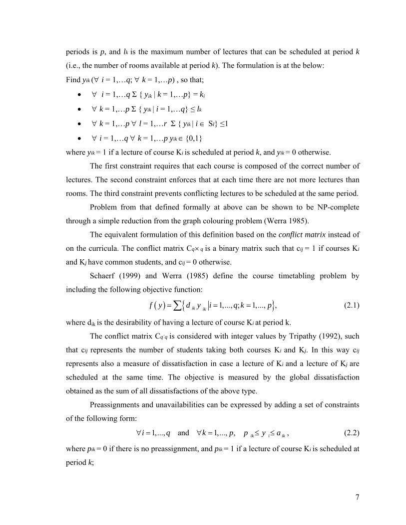
periods is p, and lk is the maximum number of lectures that can be scheduled at period k

(i.e., the number of rooms available at period k). The formulation is at the below:

Find yik (∀ i = 1,…q; ∀ k = 1,…p) , so that;

• ∀ i = 1,…q Σ yik | k = 1,…p = ki

• ∀ k = 1,…p Σ yik | i = 1,…q ≤ lk

• ∀ k = 1,…p ∀ l = 1,…r Σ yik | i ∈ Sl ≤1

• ∀ i = 1,…q ∀ k = 1,…p yik ∈0,1

where yik = 1 if a lecture of course Ki is scheduled at period k, and yik = 0 otherwise.

The first constraint requires that each course is composed of the correct number of

lectures. The second constraint enforces that at each time there are not more lectures than

rooms. The third constraint prevents conflicting lectures to be scheduled at the same period.

Problem from that defined formally at above can be shown to be NP-complete

through a simple reduction from the graph colouring problem (Werra 1985).

The equivalent formulation of this definition based on the conflict matrix instead of

on the curricula. The conflict matrix Cq× q is a binary matrix such that cij = 1 if courses Ki

and Kj have common students, and cij = 0 otherwise.

Schaerf (1999) and Werra (1985) define the course timetabling problem by

including the following objective function:

( ) 1,..., ; 1,..., ,ik ikf y d y i q k= = = p∑ (2.1)

where dik is the desirability of having a lecture of course Ki at period k.

The conflict matrix Cq´q is considered with integer values by Tripathy (1992), such

that cij represents the number of students taking both courses Ki and Kj. In this way cij

represents also a measure of dissatisfaction in case a lecture of Ki and a lecture of Kj are

scheduled at the same time. The objective is measured by the global dissatisfaction

obtained as the sum of all dissatisfactions of the above type.

Preassignments and unavailabilities can be expressed by adding a set of constraints

of the following form:

(2.2) 1,..., and 1,..., , ,ik i iki q k p p y a∀ = ∀ = ≤ ≤

where pik = 0 if there is no preassignment, and pik = 1 if a lecture of course Ki is scheduled at

period k;

7

• aik = 0 if a lecture of course Ki cannot be scheduled at period k,

• aik = 1 if a lecture of course Ki can be scheduled at period k.

De Werra (1985) shows how to reduce a course timetabling problem to graph

colouring: Associate to each lecture li of each course Kj a vertex mij; for each course Kj

introduce a clique between vertices mij (for i = 1,…q). Introduce all edges between the

clique for Kj1 and the clique Kj2 whenever Kj1 and Kj2 are conflicting.

If unavailability occurs, introduce a set of p new vertices, each one corresponding to

a period. The new generated vertices are all connected each other. This ensures that each

one is assigned to a different colour. If a course cannot have lectures at a given period, then

all the vertices corresponding to the lectures of the course are connected to a vertex

corresponding to the given period. On the other hand, if a lecture should take place at a

given time, then the vertex corresponding to that class is connected to all period vertices

but the one representing the given period.

2.3. Problem Solving

In the beginning years of timetabling research, direct heuristic methods were

applied to timetabling problems. It is focused on ordering the most urgent variables. To this

problem, look-ahead techniques (variable and value ordering heuristics) are used which

include analysis of time and object constraints. Simple, problem specific heuristic methods

can produce desirable timetables, but the size and complexity of university timetabling

problems has started a trend towards more general problem solving algorithms.

In recent years, using meta heuristic methods is proved to give better results, such

as simulated annealing, tabu search techniques. Constraint Logic Programming is also a

popular approach.

The solution approaches for timetabling problems are categorized in the following

parts.

8

2.3.1. Operations Research

It ranges from mathematical programming to heuristics, such as graph colouring

and network flow techniques. The graph colouring problem is the most known and a well

research method.

Briefly defined, graph colouring problem is to colour the vertices of a graph

, where nvvvV ,...,, 21= is the set of vertices, and E is the set of edges that

connects the vertices to find a c N⎯→⎯ such that connected vertices always

have different colours. Finding the minimum number of K, such that a feasible K colouring

exists, is the optimal solution.

EVG ,=

ng VC :olouri

To implement this method to the timetabling problems, a simple form can be

generated, where each node represents a task, each colour represents a timeslot, and each

edge ( )ji v, indicates that vv i and vj should not be placed within the same timeslot.

The graph colouring method gives good results in small scale problems. However,

in big scale problems, this method fails. Hence the real timetabling problem is a large scale

problem; more effective methods should be used.

2.3.2. Human Machine Interaction

It finds an initial feasible solution; subsequently it improves this initial solution

manually. This process iterates until the user satisfy with the result or no further

improvement can be obtained. Mulvey (1992) proposes “approximation, evaluation and

modification” model for Human Machine Interaction.

The major drawback of this method is its computationally expensiveness for large

problems (Gunadhi, et al. 1996).

9

2.3.3. Artificial Intelligence

It uses various meta-heuristic methods, for instance, simulated annealing

(Abramson 1991a), tabu search (Hertz 1992, Costa 1994), genetic algorithms (Abramson

and Abela 1991b, Burke, et al. 1994, Terashima and Marin 1998), constraint satisfaction

problem (Brittan and Farlet 1971, Jaffar and Maher 1994, Gueret, et al. 1996, Lajos 1996,

Deris, et al. 1997, Abdennadher, et al. 2000) that have been used to solve various

educational timetabling problems.

2.3.3.1. Genetic Algorithms

The logic beneath the Genetic Algorithms is the principles of evolutionary biology,

such as inheritance, mutation and natural selection. Genetic Algorithms mimic the process

of natural selection and can be used as technique for solving complex optimization

problems, which have very large search spaces.

The definition is taken from (Burke, et al. 1994): A genetic algorithm is starts by

generating a set (population) of timetables randomly. These are then evaluated according to

some sort of criteria. On the basis of this evaluation population members (timetables) are

chosen as parents for the next generation of timetables. By weighting the selection process

in favour of the better timetables, the worse are eliminated while at the same time the

search is directed towards the most promising areas of the search space.

2.3.3.2. Tabu Search

In global optimization problems based on multi level memory managment and

response exploration, tabu search can be applied. Glover (1986) described Tabu Search as

“a meta heuristic superimposed on another heuristic method”. This method is applied to

timetabling problems by Hertz (1992) and Costa (1994). Unfortunately, the tabu search is

not a very suitable technique for a big timetabling problem space.

10

2.3.3.3. Simulated Annealing

The detailed description of Simulated Annealing is mentioned in Chapter 4.

It is hard to compare these mentioned methods at above, because the problem can

response differently to different solution techniques. According to the problem

characteristics, most appropriate method should be selected. Due to timetabling problem is

NP complete problem, the running time grows exponentially as the problems size grows, so

it causes a considerable computational costs.

This thesis is concerned with the implementation of meta heuristics techniques

including constraint satisfaction problem (CSP) and simulated annealing (SA) techniques.

These methods are detailed defined in following chapters.

11

CHAPTER 3 Equation Chapter 0 Section 3

CONSTRAINT SATISFACTION PROBLEM

3.1. Historical Perspective

Constraint Satisfaction originated in the field of artificial intelligence in the 1970s.

During the 1980s and 1990s, constraints were embedded into a programming language.

Prolog and C++ are the most used languages for constraint programming.

The CSP was first formalized in line labelling in vision research. Huffman (1971),

Clowes (1971), Waltz (1975) and Mackworth (1992) define CSPs with finite domains as

finite constraint satisfaction problems, and gives a shape to CSP problems. Haralick (1979)

and Shapiro (1980) discuss different views of the CSP from problem formalization,

applications to algorithms. Meseguer (1989) and Kumar (1992) both give concise and

comprehensive overviews to CSP solving. Guesgen and Hertzberg (1992) introduce the

concept of dynamic constraints that are themselves subject to constraints. This idea is very

useful in spatial reasoning.

Mittal and Falkenhainer (1990) extend the standard CSP to dynamic CSPs (CSPs in

which constraints can be added and relaxed), and proposed the use of assumption based

TMS (ATMS) to solve them (de Kleer 1986, de Kleer 1989). Definitions on graphs and

networks are mainly done by Carré (1979). CSP was first applied to university timetabling

problems (Brittan and Farley 1971).

3.2. Definition of the Constraint Satisfaction Problem

Constraint Satisfaction Problems (CSPs) appear in many parts of the real life, for

example, vision, resource allocation in scheduling and temporal reasoning. The CSP is a

popular research topic because it is a general problem that has unique features which can be

accomplished to arrive at solutions.

12

Fundamentally, a CSP is a problem composed of a finite set of variables, each of

which is associated with a finite domain, and a set of constraints that restricts the values

the variables can simultaneously take. The task is to assign a value to each variable

satisfying all the constraints (Tsang 1993).

Formally speaking, definition of the CSP taken from Tseng’s description is as the

following:

A constraint satisfaction problem is a triple (Z, D, C) where Z is a finite set of

variables x1, x2, ..., xn, D is a function which maps every variable in Z to a set of objects

of arbitrary type, D: Z is finite set of objects (of any type). Dxi is taken as the set of objects

mapped from xi by D. These objects are called possible values of xi and the set Dxi the

domain of xi. C is a finite (possibly empty) set of constraints on an arbitrary subset of

variables in Z. In other words, C is a set of sets of compound labels. CSP (P) is used for the

symbolization that P is a constraint satisfaction problem.

Each constraint Ci involves some subset of the variables and specifies the allowable

combinations of values for that subset. A state of the problem is defined by an assignment

of values to some or all of the variables, xi = vi; xj = vj,.... An assignment that does not

violate any constraints is called a consistent or legal assignment. A complete assignment is

one in which every variable is mentioned, and a solution to a CSP is a complete assignment

that satisfies all the constraints.

Practically, for many constraint satisfaction problems it is hard or even impossible

to find a solution that assigns all the variables without any violation of the constraints of the

problem. For example, for over constrained problems, there does not exist any complete

solution satisfying all the constraints. Therefore other definitions of problem solution like

Partial Constraint Satisfaction were introduced by Freuder et al. (1992). Before mentioning

specific solution approaches for over constrained problems, it is worthy to introduce the

general solution techniques for constraint satisfaction problems.

13

3.3. Problem Solving Methods

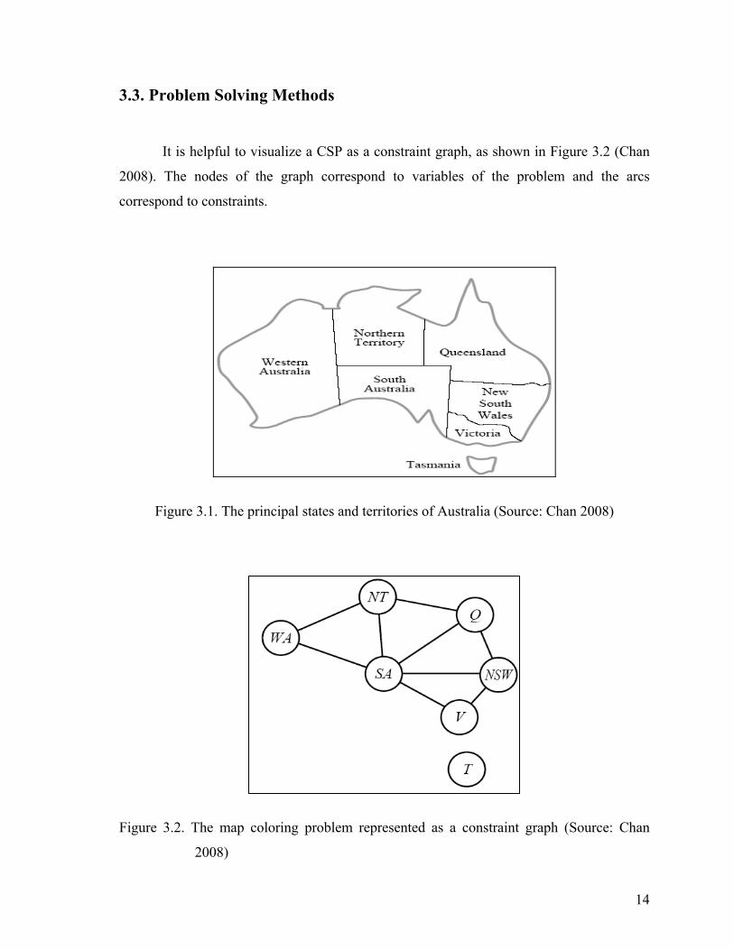
It is helpful to visualize a CSP as a constraint graph, as shown in Figure 3.2 (Chan

2008). The nodes of the graph correspond to variables of the problem and the arcs

correspond to constraints.

Figure 3.1. The principal states and territories of Australia (Source: Chan 2008)

Figure 3.2. The map coloring problem represented as a constraint graph (Source: Chan

2008)

14

In Figure 3.1 colouring the map can be viewed as a constraint satisfaction problem.

The aim is to assign colours to each region so that no neighbouring regions have the same

colour.

The goal of the problem is to find Romania at the map of Australia, shown in Figure

3.1. The task is colouring each region red, green, or blue in such a way that no

neighbouring regions have the same colour. To formulate this as a CSP, the variables are

defined to be the regions: WA, NT, Q, NSW, V, SA, and T. The domain of each variable is

the set red, green, blue. The constraints require neighbouring regions to have distinct

colours; for example, the allowable combinations for WA and NT are the pairs,

(red, green), (red, blue), (green, red), (green, blue), (blue, red), (blue, green).

The constraint can also be represented more concisely as the inequality WA≠NT,

provided the constraint satisfaction algorithm has some way to evaluate such expressions.

There are many possible solutions, such as,

WA=red, NT =green, Q=red, NSW =green, V =red, SA=blue, T =red.

3.3.1. Consistency Techniques

In constraint satisfaction problems there are specific methods related with variables,

their domains and the constraints. To understand these relations some special notation

should be known. At the below there are some definitions to make easier to understand the

solving approaches for CSPs (Tsang 1993).

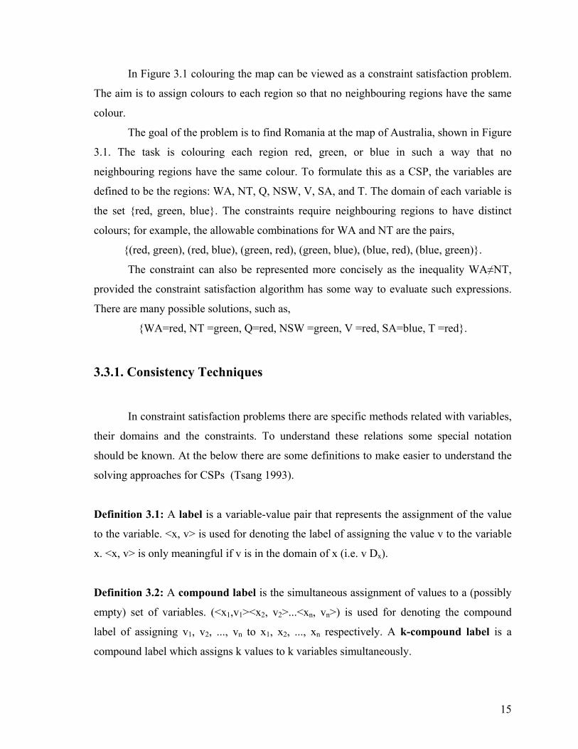
Definition 3.1: A label is a variable-value pair that represents the assignment of the value

to the variable. <x, v> is used for denoting the label of assigning the value v to the variable

x. <x, v> is only meaningful if v is in the domain of x (i.e. v Dx).

Definition 3.2: A compound label is the simultaneous assignment of values to a (possibly

empty) set of variables. (<x1,v1><x2, v2>...<xn, vn>) is used for denoting the compound

label of assigning v1, v2, ..., vn to x1, x2, ..., xn respectively. A k-compound label is a

compound label which assigns k values to k variables simultaneously.

15

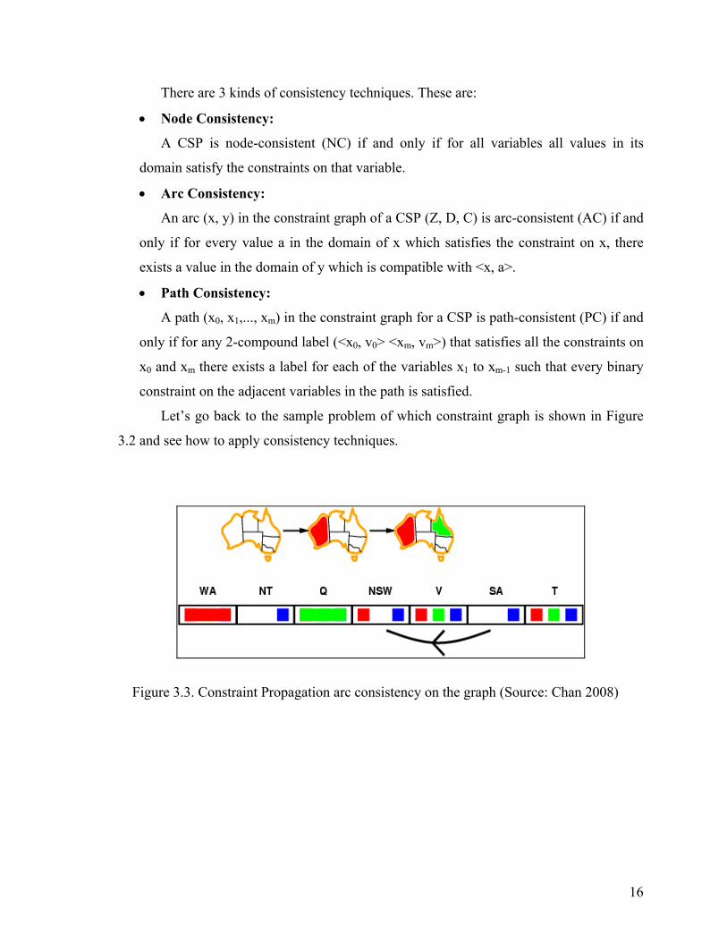
There are 3 kinds of consistency techniques. These are:

• Node Consistency:

A CSP is node-consistent (NC) if and only if for all variables all values in its

domain satisfy the constraints on that variable.

• Arc Consistency:

An arc (x, y) in the constraint graph of a CSP (Z, D, C) is arc-consistent (AC) if and

only if for every value a in the domain of x which satisfies the constraint on x, there

exists a value in the domain of y which is compatible with <x, a>.

• Path Consistency:

A path (x0, x1,..., xm) in the constraint graph for a CSP is path-consistent (PC) if and

only if for any 2-compound label (<x0, v0> <xm, vm>) that satisfies all the constraints on

x0 and xm there exists a label for each of the variables x1 to xm-1 such that every binary

constraint on the adjacent variables in the path is satisfied.

Let’s go back to the sample problem of which constraint graph is shown in Figure

3.2 and see how to apply consistency techniques.

Figure 3.3. Constraint Propagation arc consistency on the graph (Source: Chan 2008)

16

Y is consistent iff for

every v

ng arcs can

become

ach

ssignment. It’s like sending messages to neighbors on the graph.

This

ethod is repeated until convergence. (No message will change any domains.)

ain means no solution possible at all. (Back out of that branch.)

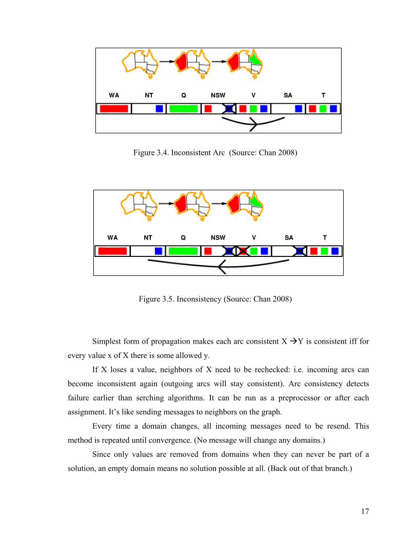
Figure 3.4. Inconsistent Arc (Source: Chan 2008)

Figure 3.5. Inconsistency (Source: Chan 2008)

Simplest form of propagation makes each arc consistent X

alue x of X there is some allowed y.

If X loses a value, neighbors of X need to be rechecked: i.e. incomi

inconsistent again (outgoing arcs will stay consistent). Arc consistency detects

failure earlier than serching algorithms. It can be run as a preprocessor or after e

a

Every time a domain changes, all incoming messages need to be resend.

m

Since only values are removed from domains when they can never be part of a

solution, an empty dom

17

3.3.2. Basic Search Strategies for the Constraint Satisfaction Problem

gies;

logical backtracking strategy and the iterative broadening

search

through constraint propagation. Such strategies exploit the fact that

variabl erated in a case analysis), and

that co

ependency-directed backtracking (DDBT), learning

nogood

n of the problem. BackJumping

as introduced in (Gaschnig 1979a).

All strategies that mentione at the above, it is assumed that the variables and values

the algorithms could be significantly affected

y the order in which the variables and values are picked.

Some of the best known search algorithms for CSPs can be classified and

summarized as:

• General Search Strate

This includes the chrono

(IB). These strategies were developed for general applications, and do not make use

of the constraints to improve their efficiency. Iterative Broadening (IB) was introduced by

Ginsberg and Harvey (1990).

• Lookahead Strategies;

The general lookahead strategy is that following the commitment to a label, the

problem is reduced

es and domains in CSPs are finite (hence can be enum

nstraints can be propagated. Algorithms which use lookahead strategies are forward

checking (FC), directional arc-consistency lookahead (DAC-L) and arc consistency

lookahead (AC-L).

• Gather Information While Searching Strategies;

The strategy is to identify and record the sources of failure whenever backtracking

is required during the search, i.e. to gather information and analyse them during the search.

Doing so allows one to avoid searching futile branches repeatedly. This strategy exploits

the fact that sibling subtrees are very similar to each other in the search space of CSPs. The

algorithms that this strategy uses are d

compound labels (LNCL), backchecking (BC) and backmarking (BM). Prosser

(1993) describes a number of jumping back strategies, and illustrates the fact that in some

cases backjumping may become less efficient after reductio

w

are ordered randomly. In fact, efficiency of

b

18

3.3.3.

uned. Besides, when the

compat

orderings, which could

lead to ktrack, it is only

use

• of the

• oiting the structure of

lure could be detected as soon as possible;

•

the fewest “legal” values is the fail first

Value and Variable Ordering

The ordering in which the variables are labelled and the values chosen affects the

number of backtracks required in a search, which is one of the most important factors

affecting the efficiency of an algorithm. In lookahead algorithms, the ordering in which the

variables are labelled also affects the amount of search space pr

ibility checks are computationally expensive, the efficiency of an algorithm could be

significantly affected by the ordering of the compatibility checks.

By appliying ordering variable methods to searching algorithms, in lookahead

algorithms, failures could be detected earlier under some orderings than others, larger

portions of the search space can be pruned off under some orderings than others. In learning

algorithms, smaller nogood sets could be discovered under certain

the pruning of larger parts of a search space. When one needs to bac

ful to backtrack to the decisions which have caused the failure.

The variable ordering techniques are as listed below (Tsang 1993):

The minimal width ordering (MWO) heuristic: By exploiting the topology

nodes in the primal graph of the problem, the MWO heuristic orders the variables

before the search starts. The intention is to reduce the need for backtracking.

The minimal bandwidth ordering (MBO) heuristic: By expl

the primal graph of the problem, the MBO heuristic aims at reducing the number of

labels that need to be undone when backtracking is required;

• The fail first principle (FFP): The variables may be ordered dynamically during the

search, in the hope that fai

The maximum cardinality ordering (MCO) heuristic: MCO can be seen as a crude

approximation of MWO.

Let’s continue over the mentioned sample problem in Figure 3.1. To make less

tracking to the back in the used search algorithm, the variable and the value selection

should be done well. For example, after the assignments for WA=red and NT =green, there

is only one possible value for SA, so it makes sense to assign SA=blue next rather than

assigning Q. In fact, after SA is assigned, the choices for Q, NSW, and V are all forced.

This intuitive idea, choosing the variable with

19

princib

l arrive at a solution

with no

to be found to a problem, not just the first one, then the ordering

oes not matter because every value should be considered. The same holds if there are no

3.4. O

efined in terms

of som

le. Starting from the most constrained variable causes a failure soon, thereby the

search tree is pruned at beginning of the search.

On the other hand, The FFP heuristic may not always help at all in choosing the first

region to color in Australia, because in the beginning, every region has three legal colors.

In this case, the degree heuristic comes in handy. It attempts to reduce the branching factor

on future choices by selecting the variable that is involved in the largest number of

constraints on other unassigned variables. In Figure 3.1, SA is the variable with the highest

degree, 5; the other variables have degree 2 or 3, except for T, which has 0. In fact, once

SA is chosen, applying the degree heuristic (MBO) solves the problem without any false

steps. Any consistent color cen be chosen at each choice point and stil

backtracking. The minimum remaining values (FFP) heuristic is usually a more

powerful guide, but the degree heuristic can be useful as a tie-breaker.

Once a variable has been selected, the algorithm should decide on the order in

which to examine its values. So that the least constraining value heuristic can be effective

in some cases. It prefers the value that rules out the fewest choices for the neighboring

variables in the constraint graph. For example, suppose that in Figure 3.1 the partial

assignment are generated with WA=red and NT =green, and the next choice is for Q. Blue

would be a bad choice, because it eliminates the last legal value left for Q’s neighbor, SA.

The least constraining value heuristic therefore prefers red to blue. In general, the heuristic

is trying to leave the maximum flexibility for subsequent variable assignments. Of course,

if all the solutions are tried

d

solutions to the problem.

ptimization Problems

In applications such as industrial scheduling, some solutions are better than others.

In other cases, the assignment of different values to the same variable incurs different costs.

The task in such problems is to find optimal solutions, where optimality is d

e application specific functions. These problems are called Constraint Satisfaction

Optimization Problems (CSOP) to distinguish them from the standard CSP.

20

Not every CSP is solvable. In many applications, problems are mostly over

constrained. When no solution exists, there are basically two things that one can do. One is

to relax the constraints, and the other is to satisfy as many of the requirements as possible.

The latter solution could take different meanings. It means labelling as many variables as

possible without violating any constraints. It also means labelling all the variables in such a

way that as few constraints are violated as possible. Such compound labels are actually

useful for constraint relaxation because they indicate the minimum set of constraints which

need to

d, where the variables are possibly weighted by their importance or for minimizing

the num

These are optimization problems, which are different from the standard CSPs

Definition 3.3: A partial constraint sa oblem (PCSP) is a quadruple (Tsang

here (Z, D, C) is a CSP, and g is a function which m

n:

ined above, since the set of solution tuples is a

bset of the compound labels. In a maxim

equival

be violated. Furthermore, weights could be added to the labelling of each variable

or each constraint violation.

In other words, the problems can be for maximizing the number of variables

labelle

ber of constraints violated, where the constraints are possibly weighted by their

costs.

defined previouly in this chapter. This class of problems is called the Partial CSP (PCSP).

tisfaction pr

1993):

(Z, D, C, g)

w aps every compound label to a

numerical value, i.e. if cl is a compound label in the CSP the

g : cl numerical value→ (3.1)

Given a compound label cl, g(cl) is called the g-value of cl.

The task in a PCSP is to find the compound label(s) with the optimal g-value with

regard to some (possibly application-dependent) optimization function g. The PCSP can be

seen as a generalization of the CSOP def

su ization problem, a PCSP (Z, D, C, f) is

ent to a CSOP (Z, D, C, g) where:

( ) ( )( )( )

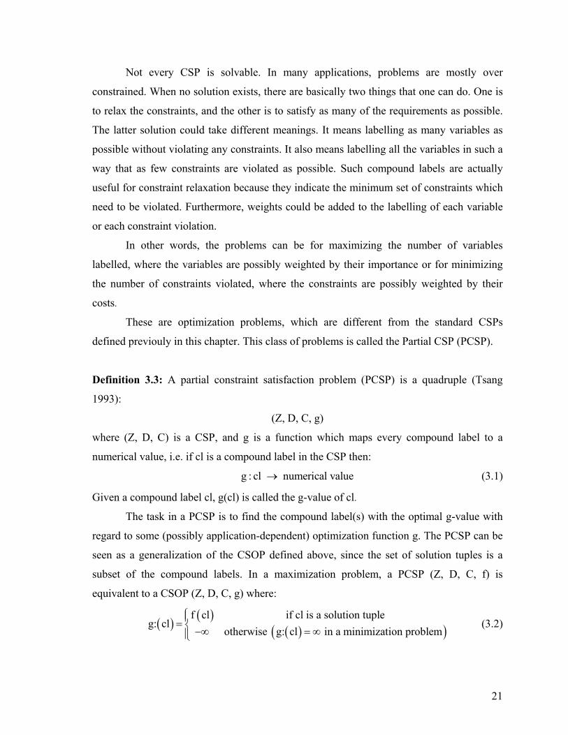
f cl if cl is a solution tupleg: cl

otherwise g: cl in a minimization problem⎧⎪= ⎨ −∞ = ∞⎪⎩

(3.2)

21

Branch and bound (B&B) is the most used optimization algorithm for solving

CSOPs. However, since CSPs are NP-complete in general, complete search algorithms may

not be

maximal utility problem

(MUP), which are motivated by scheduling applications that are normally over constrained

(Tsang 1993). Freuder and Wallace (1992) define the problem of “satisfying as many

constraints as possible” as the maximal constraint satisfaction problem and tackle it by

extending standard constraint satisfaction techniques.

able to solve very large CSOPs. Preliminary research suggests that genetic

algorithms (GAs) can be able to tackle large and loosely constrained CSOPs where near

optimal solutions are acceptable. Tsang and Warwick (1990) report preliminary but

encouraging results on applying GAs to CSOPs.

The CSOP can be seen as an instance of the partial constraint satisfaction problem

(PCSP), a more general problem in which every compound label is mapped to a numerical

value. Freuder (1989) gives the first formal definition to the PCSP. Two other instances of

PCSPs are the minimal violation problem (MVP) and the

22

CHAPTER 4 Equation Chapter 0 Section 4

SIMULATED ANNEALING

Simulated Annealing (SA) is a heuristic algorithm for the global optimization

problems. Its name and inspiration comes from the physical process of annealing in

metallurgy, which involves the collection of many particles in a physical system as it is

cooled.

The method was an adaptation of the Metropolis-Hastings algorithm, a Monte Carlo

method to generate sample states of a thermodynamic system, invented by Metropolis et al.

(1953). The first complete Simulated Annealing optimization method was searched by

Kikpatrick et al. (1982).

In 1982 Cérny developed independently an simulation algorithm based on

thermodynamics which has been called later Simulated Annealing, too. However he did not

publish his work until 1984, two years after Kirkpatrick.

4.1. Physical Background

In the simulated annealing (SA) method, each point s of the search space is

analogous to a state of some physical system, and the function E(s) to be minimized is

analogous to the internal energy of the system in that state. The task is to bring the system,

from an arbitrary initial state, to a state with the minimum possible energy.

Simulated Annealing algorithm is based on the annealing process in the physics of

solids. In this physical process, the solid is first heated to a high temperature and then

cooled slowly down to the original temperature. The high temperature provides the particle

of the solid with a very high mobility. Hence, the particles can reach locations all around

the solid. If the temperature is decreased slowly enough, all the particles of the solid

arrange themselves such that the system will have minimal bounding energy.

23

In the physics of the solids, the particles of the solid are characterized by the

probability PE of being in a state with energy E at the temperature T. The probability is

given by the Boltzman distribution:

( )1 s

z

ek TP E e

Z T

−⎛ ⎞= ×⎜⎜

⎝ ⎠⎟⎟ (4.1)

where kB is the Boltzmann constant and Z(T) is a temperature dependent normalization

factor. It is more reasonable that the particles of the system are in high energy states at high

temperatures than at lower temperatures (Metropolis, et al. 1953).

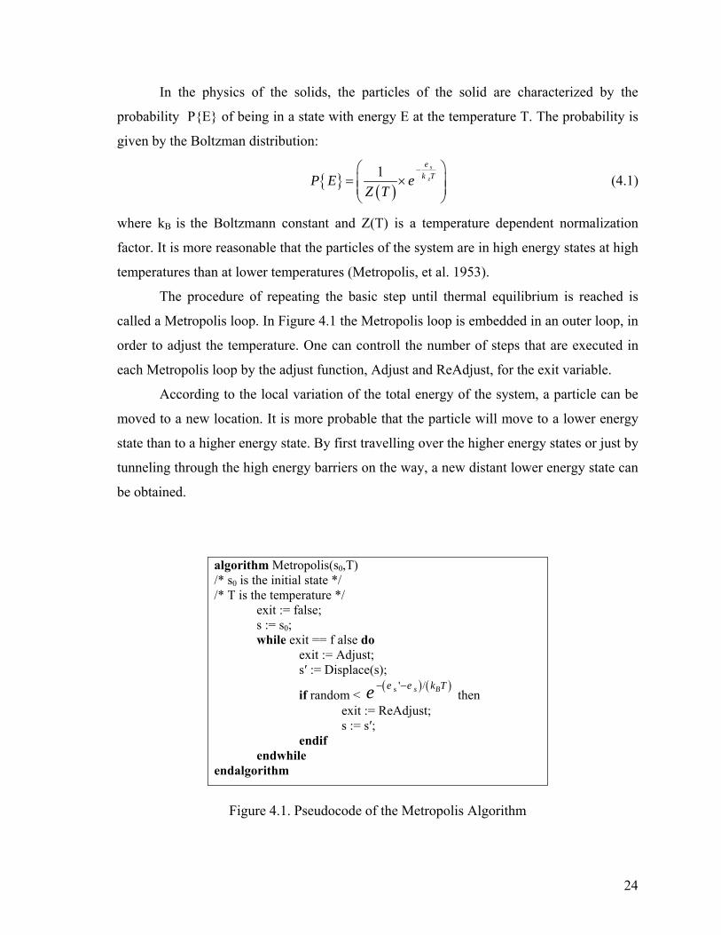
The procedure of repeating the basic step until thermal equilibrium is reached is

called a Metropolis loop. In Figure 4.1 the Metropolis loop is embedded in an outer loop, in

order to adjust the temperature. One can controll the number of steps that are executed in

each Metropolis loop by the adjust function, Adjust and ReAdjust, for the exit variable.

According to the local variation of the total energy of the system, a particle can be

moved to a new location. It is more probable that the particle will move to a lower energy

state than to a higher energy state. By first travelling over the higher energy states or just by

tunneling through the high energy barriers on the way, a new distant lower energy state can

be obtained.

algorithm Metropolis(s0,T) /* s0 is the initial state */ /* T is the temperature */ exit := false; s := s0; while exit == f alse do exit := Adjust; s′ := Displace(s);

if random < ( ) ( )s 'e− − /s Be k T

e thenust; exit := ReAdj

s := s′; endif

le endwhiendalgorithm

Figure 4.1. Pseudocode of the Metropolis Algorithm

24

4.2. Mathematical Model

Algorithm of an annealing works on a state space, which is a set with a relation. The

elements of the set are called states. Each state represents a configuration. S is denoted to

state space and its cardinality is shown by |S|. A cost function,∈: S→R+, assigns a positive

real number to each state. This number is explained as a quality indicator. The lower is

chosen this number; the better is the configuration that is encoded in that state. By defining

a neighbor relation over S, ω ⊆ S×S, called a topology, is endowed to the state set S. The

elements of ω are called moves, and the states (s, s′)∈ ω connected via a single move are

called neighbors. Similarly, the states (s, s′) ∈ ω k are said to be connected via a set of k

moves. Due to it is wanted that any state to be connected to any other state by a finite

number of moves, it is required the transitive closure of ω to be the universal relation of S:

1

.k

k

S Sω∞

=

= ×U (4.2)

4.2.1. Transitions

As already mentioned, the annealing algorithm operates on a state space. At the end

of the execution of a step exactly one state is the current state. The probability that a given

state will be the current state depends only on its cost, the cost of the previous state and the

value of the control parameter i.e., the temperature, T. The theoretical model for describing

the sequences of current states generated by the annealing algorithm is known as a Markov

chain. The essential property of Markov chains is that the next state does not depend on the

states that have preceded the current state (Feller 1950, Isaacson and Madsen 1976, Seneta

1981). The probability that s′ will be the next state, given that s is the current state is

denoted by τ (s, s′, T) and is called the transition probability. The transition probabilities

for a certain value of T can be conveniently represented by a matrix P(T), the transition

matrix. The transition matrix of the Metropolis loop does not change from step to step,

because T does not change. Markov chains with constant transition matrices are called

25

homog

he sum of all transition probabilities with that state as first state is one, because

ere is always exactly one current state. The

erefore;

eneous. The Metropolis loop can therefore be modeled by a homogeneous Markov

chain.

The transition probabilities of the states that are not connected by a move is zero.

For other pairs of distinct states, the probability is determined by the probability that, given

the first state, the second one is selected, and the probability that, once selected, the second

state is accepted as the next state. The probability that the state does not change has to be

such that t

th complete Markov model for the annealing is

th

( )s''

α(ε(s),ε(s'),T) (s, s') if s s', ', 1 α(ε(s),ε(s''),T) (s, s'') otherwises s T

βτ β

≠⎧⎪= ⎨ −⎪⎩

∑ (4.3)

where α is the acceptance probability function, and β is the selection probability function.

ote the selection probability is never ze

ove. Another function, called the acceptance function, assigns a positive probability

measure to a pair of costs, and a positive real number, the temperature. Therefore,

N ro for a pair of states connected by a single that

m

α

should be chosen in the values of; 3: (0,1] .R Rα + ⎯⎯→ ⊂ (4.4)

bility to be in a state with the

minimu

is called convergence. Briefly, the algorithm is defined to be

onvergent if the global minimum is found with certainty.

For finite search spaces S, an efficient condition for convergence is detailed balance

(Otten, et al. 1989), requiring that the probability flows between any two states si, sj in the

4.2.2. Convergence to Optimum

In the years of 1980s, several researchers independently proved that it is possible to

design a simulated annealing algorithm so that the proba

m cost approaches one as the temperature approaches zero (S. German and D.

German 1984, Gidas 1984, Gelfand and Mitter 1985, Lundy and Mees 1986, Mitra, et al.

1986). This property

c

state space are equal:

26

( ) ( ) ( ) ( )jiT (4.5)

i ij jT T Tπ τ π τ• = •

where iπ ( )T is the stationary probability d stribution of the state at temperature T. The

stationary probability distribution is a vector

i si

( ) ( ) ( ) ( )( )TTTT sππππ ,...,, 21= which satisfies

the equation

( ) ( ) ( )TT T P T Tπ π• = (4.6)

where P(T) is the transition matrix and Tπ is the transpose of π . In ot er words, the

stationary probability distribution is a left eigenvector of the transition matrix, associated

with the eigenvalue one.

Neither the existence nor the uniqueness of a stationary probability distribution is

guaranteed for a general transition matrix P. However, if the transition matrix P is

irreducible and aperiodic, then there exists a unique st tionary distribution

h

a π (Motwani, et

al. 1995). A transition matrix P(T) is irreducible if its underlying search space graph is

rongly connected and, for all si ∈ S and sj∈ iΩst , Pij(T) > 0 (Romeo, et al. 1991). The

tran i iodic if its underlying search space graph has no state to sit on matrix is called aper

which the search process will continually return with a fixed time period. A sufficient

condition for aperiodicity is that there exist a state si∈S such that Pii ≠ 0 (Romeo, et al.

991).

oof o onvergence

imum requ

1

• Pr f C

If the global minimum is reachable from the initial configuration then the algorithm

can be called as convergent. Finding the global min ires that;

1lim i opti

x R⎯⎯→∞

∈ = (4.7)

where xj can be reachable from a configuration xi if there exists a path xi, xi+1, xi+2,… xi+n = xj

for some 0≥n .

Let the probability to generate a configuration x be ( )ksxg , at temperature Tk and

the probability of not generating the configuration be ( )ksx,g1− . The subscript k denotes

e index of the cooling cycle. th

27

The global minimum is found with certainty if there is a possibility that every

possible combination of optimization variables x is generated at each temperature. To be

re that every possible combination of optimization variables is generated at least once

n arbitrary configuration vanishes. That leads

satisfying equation;

su

requires that the possibility of not generating a

to

( , )o

kk k

g x s∞

=

= ∞∑ (4.8)

which can be said that every possible combination is visited infinitely often in time. This is

the most often used form of the proof of the convergence in Simulated Annealing.

4.3. Simulated Annealing Algorithm

In Figure 4.2, the pseudocode of the simulated annealing algorithm is given. The

particle

ntil the thermal

equilib

mum found, the loop is repeated and the loop

dex k is incremented. The system is frozen when T

s are displaced randomly with a probability function using variance s = sk at the

same temperature T = Tk as in the Monte Carlo method. The subscript k denotes the index

of the cooling cycle. Transitions at one temperature are made only u

rium is reached. After reaching the equilibrium, the temperature is lowered. If the

system is not frozen nor is the global mini

in ≤ Tf, where Tf is a user defined final

temperature.

In Figure 4.2 the variables k and l are the loop variables. l marks the iteration at

temperature Tk. k is increased after the thermal equilibrium at temperature Tk is reached.

The temperature Tk and the variance sk control the randomization process.

There are different kinds of Simulated Annealing algorithms. In this thesis the most

basic and the used methods are mentioned.

28

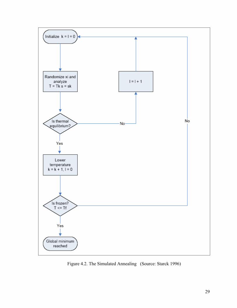
Figure 4.2. The Simulated Annealing (Source: Starck 1996)

29

4.3.1. Original Simulated Annealing

This method was dedicated to discrete optimization by Kirkpatrick et al. (1983). It

was not proven to be convergent. They used the cooling function as shown as below:

(4.9) 1k

k kT T Tα α−= = 0

where [ [1,0∈α is a scaling constant. Useful values for α have been claimed to

be 8.0 ⟨ 9.0⟨α .

SA has shown successful applications in a wide range of combinatorial optimization

roblems, and this fact has motivated researchers to use SA in simulation optimization.

.3.2. Boltzmann Annealing

ealing

ethod to the global minimum. The Gaussian

p

4

Boltzmann Annealing or Classical Simulated Annealing was studied by Geman et

al. (1984). They first gave an essential condition for the convergence of the ann

m distribution was used for one variable;

( )( ) 2

01 x x2,

2ks

kk

g x s esπ

= (4.10)

here x0 is the current value of the optimization variable x.

by;

− −

w The temperature was calculated

( )

0 , 1, ,ln 1k .T k

kT

= = ∞+

K (4.11)

If Equation 4.8, the formulation of the proof of convergence, is applied to this

algorithm;

30

( ) 20 /21( , )

i i ik

o o

n x x sk ik k k k

g x s e∞ ∞

( ) ( )

( )

1

0 1

0

2

ln 1

11

o

ik

n

ik k

s

c k e

ck

π

ln 1k− +

ln 10

o

k

k kc e

∞− +

=

− −

=

∞

==

∞

= =

= Π∑ ∑

⎡ ⎤= Π +⎢ ⎥

ok k=

⎣ ⎦

=+

∑

∑

0 constant and k0 is an arbitrary cooling cycle (Ingber, 1989). The

ript of i marks the ith dimension in the set of optim

4.3.3. Fast Annealing

This method is a semi local search and consists of occasional long jumps (Szu, et al.

1987). It is the improvement of Boltzmann Annealing method. In the fast annealing,

Cauchy distribution is used instead of Gaussian Method which is used of Boltzmann

Annealing. It can be formulated as below;

≥ ∑ (4.12)

= ∞

where c is an arbitrary

supersc ization variables x.

( ) ( ) 2 20

, .[ ]

kk

k

sg x sx x sπ

=− +

(4.13)

This distribution has higher probability for values x far from x0 than the Gaussian

distribution. Thus the probability of occasional long jumps is greater and leaving local

minima is more likely.

Another difference is the cooling schedule in Cauchy distribution. It has a faster

schedule;

0 .1kTT

k=

+ (4.14)

It is also proved to be convergent as Boltzmann method.

31

4.3.4. Very Fast Simulated Reannealing

Very Fast Simulated Reanneling algorithm permits a fast exponential cooling

schedule rather than the cooling schedules of the Fast Annealing and the Boltzmann

Annealing (Ingber, et al. 1989).

As generation probability, they defined a new density function;

( )( )

1,12 ' ln 1

k

kk

g x sx s sπ

=⎛ ⎞∆ + +⎜ ⎟⎝ ⎠

(4.15)

where 'x is a normalized step (x-x∆ 0)/(xmax-xmin). xmin is the lower limit of optimization

variable x and xmax is the upper limit. Both upper and lower limits must be given for every

optimization variable. The new generation function was needed in order to satisfy the proof

of the convergence.

For the cooling function, this method has a very fast decreasing function;

( )1/0 exp n

kT T ck= − (4.16)

where c is a scaling constant.

It is also proved to be convergent as the previous methods.

32

CHAPTER 5 Equation Chapter 0 Section 5

DESCRIPTION OF THE TIMETABLING PROBLEM AND

SOLVING METHODS

In this chapter, the timetabling problem of Computer Engineering Department of

İzmir Institute of Technology (İYTE) is defined and the solving techniques are explained.

Due to the university course timetabling problem is an optimization problem in which a set

of events has to be scheduled in timeslots and located in suitable rooms, the most suitable

methods are tried to be chosen, such as CSP and SA.

5.1. Problem Representation

As a sample case, 2007-2008 Fall Semester is handled. This problem consists of 5

classes (including postgraduate classes) with 5 classrooms and a laboratory that computer

engineering has. In this case, any constraint related with classrooms is ignored such as

capacity of the rooms or room availability, because each class has its own classroom in

computer engineering department. Totally there are 20 lectures that are given by 8

instructors in this case study as shown in Table 5.2. Lecture durations can change between

3 to 5, but the lectures that take 5 time slots are divided as 3 slots for theoretical and 2 slots

for laboratory lectures. Hence, the laboratory lessons are considered as a separate lesson of

which duration is 2 time slots and they are taken in the laboratory. There can be maximum

8 time slots for one day in İYTE, which means there are 40 time slots per week.

The aim of this thesis is to fulfill more demands of the instructors and the students

than the used course timetable of the mentioned semester. Also all the additional

constraints have to be satisfied. They are divided into two categories as mentioned in

Chapter 2; hard constraints that must be satisfied and soft constraints expressing the

preferences.

33

The hard constraints that are taken into account are listed as below;

• Each instructor can take only one class at a time.

• Clashes must not occur between the lectures for students of one class.

• If any instructor has some requests that have to be satisfied, their demands

must be fulfilled.

• If any class has to take lectures from other departments, the time slots that

are given from those departments must be allowed to those lectures.

• All lectures must start and finish in the same day.

The soft constraints that are taken into account are:

• The number of alternatives which students can attend should be maximized.

• The student conflicts between lectures should be minimized.

• Friday should be free for all classes.

• Preferences of instructors should be fulfilled.

All these constraints, hard and soft constraints of all the instructors and classes, are

given in detailed form in the Table 5.1 and Table 5.2.

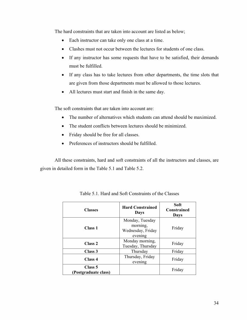
Table 5.1. Hard and Soft Constraints of the Classes

Classes Hard Constrained Days

Soft Constrained

Days

Class 1

Monday, Tuesday morning,

Wednesday, Friday evening

Friday

Class 2 Monday morning, Tuesday, Thursday Friday

Class 3 Thursday Friday

Class 4 Thursday, Friday evening Friday

Class 5 (Postgraduate class) Friday

34

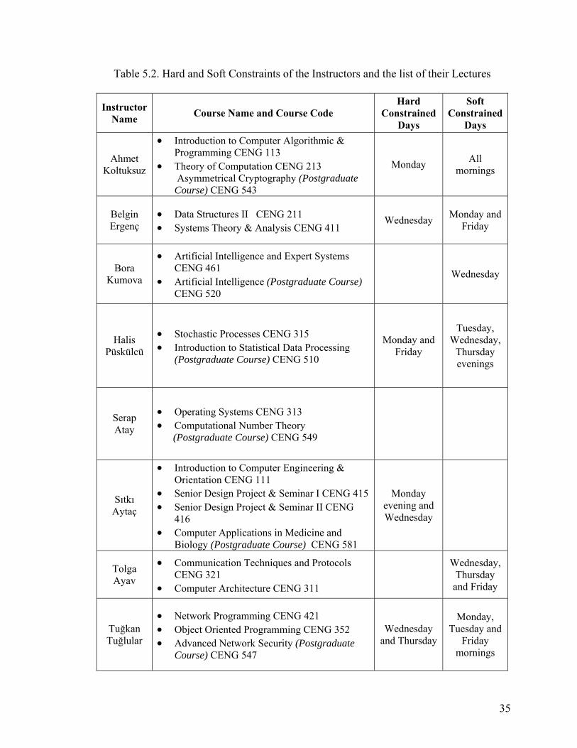
Table 5.2. Hard and Soft Constraints of the Instructors and the list of their Lectures

Instructor Name Course Name and Course Code

Hard Constrained

Days

Soft Constrained

Days

Ahmet Koltuksuz

• Introduction to Computer Algorithmic & Programming CENG 113

• Theory of Computation CENG 213 Asymmetrical Cryptography (Postgraduate Course) CENG 543

Monday All mornings

Belgin Ergenç

• Data Structures II CENG 211 • Systems Theory & Analysis CENG 411

Wednesday Monday and Friday

Bora Kumova

• Artificial Intelligence and Expert Systems CENG 461

• Artificial Intelligence (Postgraduate Course) CENG 520

Wednesday

Halis Püskülcü

• Stochastic Processes CENG 315 • Introduction to Statistical Data Processing

(Postgraduate Course) CENG 510

Monday and Friday

Tuesday, Wednesday,

Thursday evenings

Serap Atay

• Operating Systems CENG 313 • Computational Number Theory (Postgraduate Course) CENG 549

Sıtkı Aytaç

• Introduction to Computer Engineering & Orientation CENG 111

• Senior Design Project & Seminar I CENG 415 • Senior Design Project & Seminar II CENG

416 • Computer Applications in Medicine and

Biology (Postgraduate Course) CENG 581

Monday evening and Wednesday

Tolga Ayav

• Communication Techniques and Protocols CENG 321

• Computer Architecture CENG 311

Wednesday, Thursday

and Friday

Tuğkan Tuğlular

• Network Programming CENG 421 • Object Oriented Programming CENG 352 • Advanced Network Security (Postgraduate

Course) CENG 547

Wednesday and Thursday

Monday, Tuesday and

Friday mornings

35

5.2. Approaches to Solve the Problem

The approach that is taken for solving the timetabling problem of the computer

engineering department of İYTE consists of two phases, providing a hybrid method:

• Constraint Programming: It is to obtain an initial feasible timetable.

• Simulated Annealing: It is to improve the quality of the timetable.

The first phase, Constraint Programming, is used primarily to obtain an initial

timetable satisfying all the hard constraints. The second phase, Simulated Annealing, aims

to improve the quality of the timetable, taking the soft constraints into account. The method

used in the second phase is optimization method, which looks for to optimize a given

objective function.

The initialization strategy for the SA algorithm has a crucial influence on the

performance of the algorithm. So it is good to make the initial solution as good as possible

in as little time as possible. Constraint programming is a good choice for this criterion.

5.2.1. Constraint Programming Phase

Constraint Programming techniques have been studied since 1990s. Due to they

base on backtracking search, at the beginning they have been developed in Prolog, where

backtracking and declarativity had been already implemented. In this way Constraint Logic

Programming (CLP) was created as an addition to Logic Programming (LP). The languages

from this area, which are still popular, are CHIP, Sicstus, Eclips to name a few. Then CP

leaves a Prolog and comes into two branches one of them is C/C++ libraries (e.g. ILOG)

and the second is multiparadigm languages (e.g. Mozart/OZ). All of these languages have

two common features constraint propagation and distribution (labeling) connected with

search.

However, real life problems are generally over constrained and these Prolog based

programs can not be enough due to their local search techniques. For tight problems that

are normally con not satisfy all constraints, one may want to find compound labels which

36

are as close to solutions as possible, where closeness may be defined in a number of ways.

This approach is mentioned in Chapter 3, which is called Partial Constraint Satisfaction

Problems.

For all these reasons, the chosen tool to obtain the initial timetable is based on a

partial constraint solver. The constraint solver library (Muller 2005) contains a local search

based framework that allows modeling of a problem using constraint programming

primitives (variables, values, constraints).

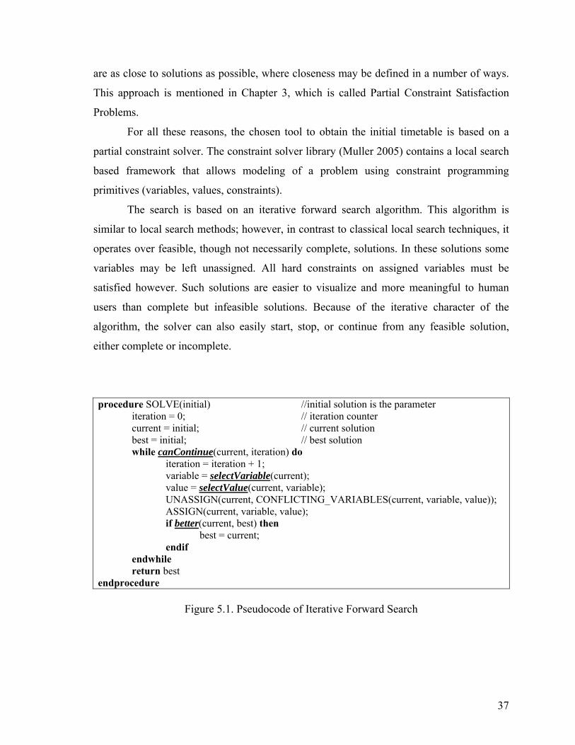
The search is based on an iterative forward search algorithm. This algorithm is

similar to local search methods; however, in contrast to classical local search techniques, it

operates over feasible, though not necessarily complete, solutions. In these solutions some

variables may be left unassigned. All hard constraints on assigned variables must be

satisfied however. Such solutions are easier to visualize and more meaningful to human

users than complete but infeasible solutions. Because of the iterative character of the

algorithm, the solver can also easily start, stop, or continue from any feasible solution,

either complete or incomplete.

procedure SOLVE(initial) //initial solution is the parameter iteration = 0; // iteration counter current = initial; // current solution best = initial; // best solution while canContinue(current, iteration) do iteration = iteration + 1; variable = selectVariable(current); value = selectValue(current, variable); UNASSIGN(current, CONFLICTING_VARIABLES(current, variable, value)); ASSIGN(current, variable, value); if better(current, best) then best = current; endif endwhile return best endprocedure

Figure 5.1. Pseudocode of Iterative Forward Search

37

As seen in the Figure 5.1, during each step, a variable X is initially selected. As in

backtracking-based searches, an unassigned variable is selected randomly. Sometimes an

assigned variable can be selected when all variables are assigned but the solution found so

far is not good enough (for example, when there are still many violations of soft

constraints). Once a variable X is selected, a value x from its domain Dx is chosen for

assignment. Even if the best value is selected, its assignment to the selected variable may

cause some hard conflicts with already assigned variables. Such conflicting assignments are

removed from the solution and become unassigned. At the end of the search, the selected

value is assigned to the selected variable.

The algorithm tries to move from one partial solution s to another via repetitive

assignment of a selected value x to a selected variable X. During this search, the feasibility

of all hard constraints in each iteration step is enforced by unassigning the conflicting

assignmentsη . The search is terminated when the requested solution is found or when there

is a timeout expressed, for example, as a maximal number of iterations or available time

being reached. If the best solution is found, it will return (Muller 2005).

The functions used in the above algorithm can be defined as (Muller 2005);

• The termination condition (function canContinue).

• The solution comparator (function better).

• The variable selection (function selectVariable).

• The value selection (function selectValue).

Structure of the Problem Modelling can be explained as below:

The model of the case study problem consists of a set of resources, a set of activities

and a set of dependencies between the activities. The time slots can be assigned a

constraint, either hard or soft; a hard constraint indicates that the slot is forbidden for any

activity, a soft constraint indicates that the slot is not preferred. These constraints are called

as “time preferences”. Time preferences can be assigned to each activity and each resource,

which indicate forbidden and not preferred time slots (Muller 2005).

38

• Activity:

The lectures are called activities in the timetabling model. Every activity is

defined by its duration (expressed as a number of time slots), by time preferences,

and by a set of resources. Activities require these set of resources. If there is a need

of resource sets one can create a resource group that the activity requires. These

resource groups can be either conjunctive or disjunctive: the conjunctive group of

resources means that the activity needs all the resources from the group, the

disjunctive group means that the activity needs one of the resources among the

alternatives. For instance, a lecture, which will take place in one of the possible

classrooms, will be taught for all of the selected classes.

• Resource:

Resources also can be described by time preferences. Only one activity can

use the resource at the same time. Each resource can represent a teacher, a class, a

classroom, or another special resource at the lecture timetabling problem.

• Dependencies:

Dependencies define and handle the relations between the activities. It

seems sufficient to use binary dependencies only those define the constraints

between the activities. There are five operators between the activities that can be

used; before; closely before; after; closely after; no conflict; concurrently. If one

activity has to start before another activity one can use “Before” constraint in the

model.

The solution of the problem defined by the above model is a timetable where every

scheduled activity has assigned its start time and a set of reserved resources that are needed

for its execution. This timetable must satisfy all the hard constraints, those defined in the

beginning of this chapter. If they are defined again according to this structure;

• Every scheduled activity has all the required resources reserved.

• Two scheduled activities cannot use the same resource at the same time.

• No activity is scheduled into a time slot where the activity or some of its

reserved resources has a hard constraint in the time preferences.

• All dependencies between the scheduled activities must be satisfied.

39

Furthermore, the number of violated soft constraints are tried to be minimized.

5.2.2. Simulated Annealing Phase

The timetable produced by the constraint programming algorithm is used as the

starting point for the simulated annealing phase of the hybrid method. This phase is used to

improve the quality of the timetable.

The application of simulated annealing to the timetabling problem is relatively

straight forward. The particles are replaced by elements. The system energy can be defined

by the timetable cost for timetable modeling. An initial allocation is made in which

elements are placed in a randomly chosen period. The initial cost and an initial temperature

are computed. To determine the quality of the solution, the cost has a critical role in the

algorithm just as the system energy role in the quality of a particle being annealed. The

temperature is used to control the probability of an increase in cost and can be likened by

the temperature of a physical particle (Abramson 1991).

The change in cost is the difference of two costs; one of them is the first cost that is

before the randomly chosen element is changed and the second one is the cost after the

randomly chosen element is changed of an activity. The element is moved if the change in

cost is accepted, either because it lowers the system cost, or the increase is allowed at the

current temperature. According to the timetabling problem model the cost of removing an

element usually consists of a class cost, an instructor cost and a room cost.

Because each class has one room, there is no room constraint in this problem. In

addition it is known that which lecture is given by which instructor. According to these

properties of the problem, the model of this studied problem is simpler than the usual ones;

the only element that can change the cost is the start times of the activities.

The typical SA algorithm accepts a new solution if its cost is lower than the cost of

the current solution. Even if the cost of the new solution is greater, there is a probability of

this solution to be accepted. With this acceptance criterion it is then possible to climb out of

local optima. The used algorithm in this study can be seen in the Figure 5.2 (Duong, et al.

2004).

40

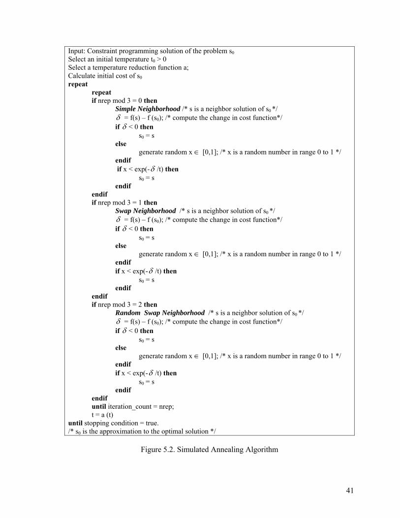
Input: Constraint programming solution of the problem s0Select an initial temperature t0 > 0 Select a temperature reduction function a; Calculate initial cost of s0repeat repeat if nrep mod 3 = 0 then Simple Neighborhood /* s is a neighbor solution of s0 */ δ = f(s) – f (s0); /* compute the change in cost function*/ if δ < 0 then s0 = s else generate random x ∈ [0,1]; /* x is a random number in range 0 to 1 */ endif if x < exp(-δ /t) then s0 = s endif endif if nrep mod 3 = 1 then Swap Neighborhood /* s is a neighbor solution of s0 */ δ = f(s) – f (s0); /* compute the change in cost function*/ if δ < 0 then s0 = s else generate random x ∈ [0,1]; /* x is a random number in range 0 to 1 */ endif if x < exp(-δ /t) then s0 = s endif endif if nrep mod 3 = 2 then Random Swap Neighborhood /* s is a neighbor solution of s0 */ δ = f(s) – f (s0); /* compute the change in cost function*/ if δ < 0 then s0 = s else generate random x ∈ [0,1]; /* x is a random number in range 0 to 1 */ endif if x < exp(-δ /t) then s0 = s endif endif until iteration_count = nrep; t = a (t) until stopping condition = true. /* s0 is the approximation to the optimal solution */

Figure 5.2. Simulated Annealing Algorithm

41

From this algorithm, in Figure 5.2, it can be seen there are several aspects of the SA

algorithm that are problem oriented. Design of a good annealing algorithm is very

important, it generally comprises three components: Neighborhood structure, cost function

and cooling schedule.

5.2.2.1. Neighbourhood Structure

In order to apply the SA algorithm a neighborhood structure which defines for each

solution a set of neighboring solutions must be included. This is the key component of any

simulated annealing method. In this thesis three algorithms are tried and all of them are

used one by one. Although they are tried to be used individually in the SA algorithm, the

most effective result is obtained when they are used together. In each iteration of SA

algorithm indexed by nrep, these three algorithms are executed in turns.

The first one of the neighbor algorithm is simple neighborhood searching. It

randomly chooses one activity and one slot. The chosen slot is assigned as the start time of

the selected activity.

The second algorithm selects randomly two activities and swaps their start times. It

is called swap neighborhood.

The third one of the neighbor algorithms chooses randomly two activities and two

slots which are referred as random swap neighborhood in this study. These two slots are

assigned as the start times of the randomly selected activities.

5.2.2.2. Cost Calculation

For the case of course scheduling, the cost calculation tries to show the influences

of both the hard constraints and soft constraints. Penalty scores of both the hard constraints

and soft constraints can be seen in the below. Each constraint is defined by a penalty score

function.

The conditions that the timetable has penalties for hard constraints are:

42

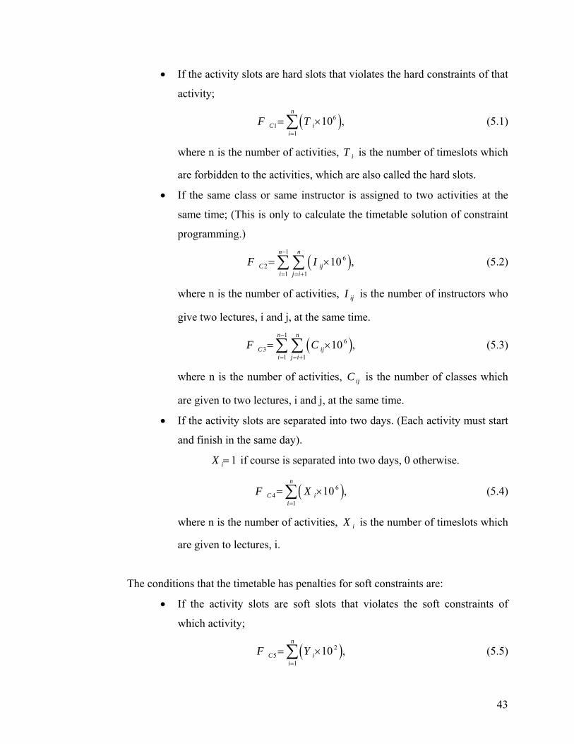
• If the activity slots are hard slots that violates the hard constraints of that

activity;

(5.1) ( 61

110 ,

n

C ii

F T=

= ×∑ )

)

)

C

• ated into two days. (Each activity must start

and finish in

if course is separa

,i=

(5.4)

where n is the number of activities, is the number of timeslots which

The condit penalties for soft constraints are:

• If the activity slots are so

n

i=

where n is the number of activities, iT is the number of timeslots which

are forbidden to the activities, which are also called the hard slots.

• If the same class or same instructor is assigned to two activities at the

same time; (This is only to calculate the timetable solution of constraint

programming.)

(5.2) (1

62

1 1

10 ,n n

C iji j i

F I−

= = +

= ×∑ ∑

where n is the number of activities, is the number of instructors who

give two lectures, i and j, at the same time.

ijI

(5.3) (1

63

1 1

10 ,n n

C iji j i

F C−

= = +

= ×∑ ∑

where n is the number of activities, ij is the number of classes which

are given to two lectures, i and j, at the same time.

If the activity slots are separ

the same day).

1=iX ted into two days, 0 otherwise.

( )64 10

n

C iF X= ×∑1

iX

are given to lectures, i.

ions that the timetable has

ft slots that violates the soft constraints of

which activity;

( )25 10 ,C iF Y= ×∑ (5.5)

1

43

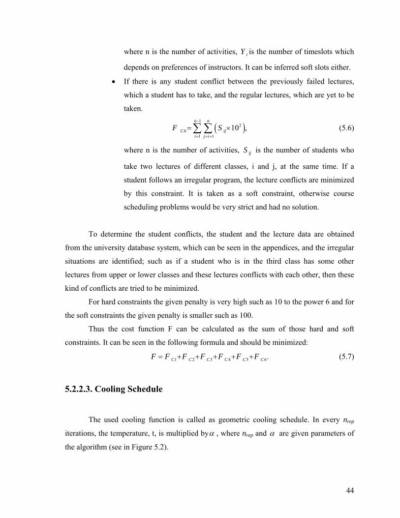
where n is the number of activities, iY is the number of timeslots which

depends on preferences of instructors. It can be inferred soft slots either.

If there• is any student conflict between the previously failed lectures,

which a student has to take

ime. If a

student follows an irregular program, the lecture conflicts are minimized

can be seen in the appendices, and the irregular

situatio

icts with each other, then these

kind of

wer 6 and for

e soft constraints the given penalty is smaller

Thus the cost function F can be calculated as the sum of those hard and soft

following formula and should be minimized:

(5.7)

, and the regular lectures, which are yet to be

taken.

( )1

26

1 110 ,

n n

C iji j i

F S−

= = +

= ×∑ ∑ (5.6)

where n is the number of activities, ijS is the number of students who

take two lectures of different classes, i and j, at the same t

by this constraint. It is taken as a soft constraint, otherwise course

scheduling problems would be very strict and had no solution.

To determine the student conflicts, the student and the lecture data are obtained

from the university database system, which

ns are identified; such as if a student who is in the third class has some other

lectures from upper or lower classes and these lectures confl

conflicts are tried to be minimized.

For hard constraints the given penalty is very high such as 10 to the po

th such as 100.

constraints. It can be seen in the

1 2 3 4 5 6.C C C C C CF F F F F F F= + + + + +

5.2.2.3. Cooling Schedule

The used cooling function is called as geometric cooling schedule. In every nrep

iterations, the temperature, t, is multiplied byα , where n and rep α are given parameters of

the algorithm (see in Figure 5.2).

44

The parameter of nrep is chosen as 3, which returns the best solution cost within an

acceptable run time. To determine nrep, several different values are experimented, namely,

1, 2, 3, 6, 10, 5.

To determine starting temperature, a rough start temperature t0 = 10000 is chosen

which

dence between the

starting acceptance probability

is hot enough to allow moves to almost neighbourhood state, and the SA algorithm

tries to derive the real start temperature T0 basing on the functional depen

0χ (70% to 80%) and the starting temperature T0.

The functional dependence between the starting acceptance probability 0χ and the

starting temperature T0 is given as follows (Poupaert and Deville 2000):

( )

( ) ( )

0 1 1 0

01

, , ,..., ,

1n n m

n

Tχ χ δ δ δ δ+= (5.8)

exp /ii

T m n mm

δ=

= − + −∑

where ( ) ( )0sfsf ii −=δ , s0 is the initial solution, si is a neighbor solution of s0, f is the cost

function, m is the size of neighbor solution space. The solution space is calculated by

(n*(n-1)/2) formulation.

For the derivation of the starting temperature T0 from the starting acceptance

probability 0χ (%70 to %80) using Equation 5.8, a small algorithm is used (Duong, et al.

2004). This algorithm has to be run only once for each execution of the SA algorithm. The

algorithm is given in Figure 5.3.

To determine the final temperature Tf, since there are no accurate recommendations

in literature, several final temperatures are experimented, namely, 0.5, 0.05,

f which returns the best solution

cost.

or the value

0.005, 0.0005, and 0.00005. Finally, 0.005 is chosen for T

45

Step 1: m := n(n-1)/2 ; /* n is the number of exams */ compute iδ , mi ≤≤1 ; t := 10000; 0 t := t ; j := 0; 0 repeat j:= j+1; t := t*j; compute ( )0tχχ = (using Equation 5.8); until 8.0≥χ ;

tep 2: exit := false; S tend := t; repeat t = (t0 + tend)/2; compute ( )tχχ = (using Equation 5.8); if 0.7 < χ < 0.8 then exit := true else if 7.0≤χ then

t0 := t if

/* t is the desired starting temperature */

tend := t else end until exit;

Figure 5.3. Algorithm to Determine Starting Temperature

To determine the reduction parameter α for geometric cooling, the formu

proposed by Burke et al. (2001) is used which allows defining a v

la

alue for the parameter α

based on the predefined time to run for the simulated annealing.

( ) ( )( )01 ln ln /f move

The ti that is wanted the SA algorithm to run for is re resented in the number of

SA steps, N

T T Nα = − − . (5.9)

me p

move. A value can be computed for the parameter α based on the predefined

time (Nmove) that the user wants the SA algorithm to run for with the fixed values for T0 and

Tf, using Equation 5.9. This mechanism is called time predefined simulated annealing

(Burke, et al. 2001). It not only helps to increase the efficiency of the SA algorithm but also

helps to make simulated annealing experiments easier.

46

CHAPTER 6 Equation Chapter 0 Section 6

CONCLUSION

In this chapter, the experimental results are evaluated and some comparisons are

done between the different initial timetable solutions. In addition, some comments on

future works that can be performed are made.

6.1. Experimental Results

The İYTE Computer Engineering Timetabling Problem is implemented with

Eclipse SDK Version 3.1.2 with Java Programming Language and experimented on an Intel

Core(TM) Duo 2.40 GHz PC.

In the first phase, the initial timetable solution of the timetabling problem is

completed in 5 minutes. The constraint solver gives the output folder for any difficulty

level of problem (can be loosen or tighten) in the same time duration.

For the second phase, simulated annealing part, the solution can be obtained in

different time durations. According to the problem difficulty and the chosen parameter

values for the SA algorithm, the execution time can change. For instance run times on the

same computer resources with the number of SA steps, Nmove, changing from 5 to 3000 are

given in the Table 6.1. As seen from the table, if the number of SA steps high enough, such

as the rate of cooling slow enough, the solution cost will improve a lot, i.e. a good quality

solution comes out, but when the number of SA steps is already too high, the solution will

not improve much (Duong, et al. 2004). Briefly, the advantage of time predefined search

algorithms over traditional local search algorithms can be explained as; in traditional local

search algorithms there are a common practice to run the algorithm several times in order to

get the best possible value of the cost function. In contrast, in time-predefined algorithms

the aim is to use all the time effectively in a single search for a high quality solution

(Burke, et al. 2001).

47

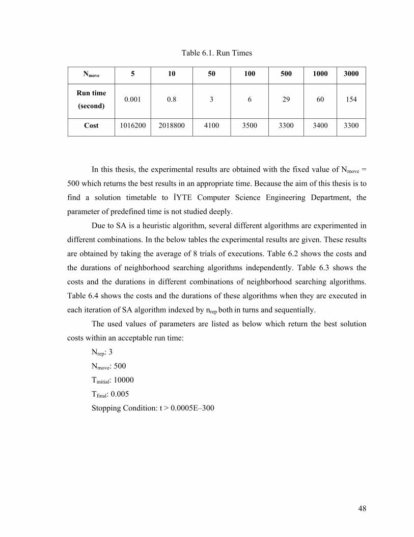
Table 6.1. Run Times

Nmove 5 10 50 100 500 1000 3000

Run time

(second) 0.001 0.8 3 6 29 60 154

Cost 1016200 2018800 4100 3500 3300 3400 3300

In this thesis, the experimental results are obtained with the fixed value of Nmove =

500 which returns the best results in an appropriate time. Because the aim of this thesis is to

find a solution timetable to İYTE Computer Science Engineering Department, the

parameter of predefined time is not studied deeply.

Due to SA is a heuristic algorithm, several different algorithms are experimented in

different combinations. In the below tables the experimental results are given. These results

are obtained by taking the average of 8 trials of executions. Table 6.2 shows the costs and

the durations of neighborhood searching algorithms independently. Table 6.3 shows the

costs and the durations in different combinations of neighborhood searching algorithms.

Table 6.4 shows the costs and the durations of these algorithms when they are executed in

each iteration of SA algorithm indexed by nrep both in turns and sequentially.

The used values of parameters are listed as below which return the best solution

costs within an acceptable run time:

Nrep: 3

Nmove: 500

Tinitial: 10000

Tfinal: 0.005

Stopping Condition: t > 0.0005E–300

48

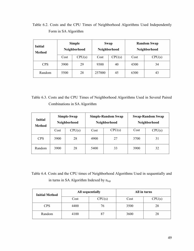
Table 6.2. Costs and the CPU Times of Neighborhood Algorithms Used Independently

Form in SA Algorithm

Simple

Neighborhood

Swap

Neighborhood

Random Swap

Neighborhood Initial

Method Cost CPU(s) Cost CPU(s) Cost CPU(s)

CPS 3900 29 9300 40 4300 34

Random 5500 28 257000 45 6300 43

Table 6.3. Costs and the CPU Times of Neighborhood Algorithms Used in Several Paired

Combinations in SA Algorithm

Simple-Swap

Neighborhood

Simple-Random Swap

Neighborhood

Swap-Random Swap

Neighborhood Initial

Method Cost CPU(s) Cost CPU(s) Cost CPU(s)

CPS 3900 28 4900 27 3700 31

Random 3900 28 5400 33 3900 32

Table 6.4. Costs and the CPU times of Neighborhood Algorithms Used in sequentially and

in turns in SA Algorithm Indexed by nrep

All sequentially All in turns Initial Method

Cost CPU(s) Cost CPU(s)

CPS 4400 76 3500 28

Random 4100 87 3600 28

49

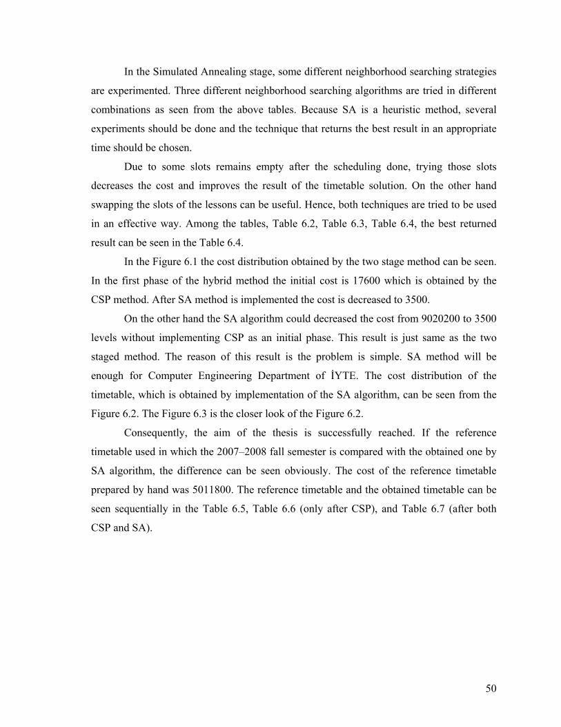
In the Simulated Annealing stage, some different neighborhood searching strategies

are experimented. Three different neighborhood searching algorithms are tried in different

combinations as seen from the above tables. Because SA is a heuristic method, several

experiments should be done and the technique that returns the best result in an appropriate

time should be chosen.

Due to some slots remains empty after the scheduling done, trying those slots

decreases the cost and improves the result of the timetable solution. On the other hand

swapping the slots of the lessons can be useful. Hence, both techniques are tried to be used

in an effective way. Among the tables, Table 6.2, Table 6.3, Table 6.4, the best returned

result can be seen in the Table 6.4.

In the Figure 6.1 the cost distribution obtained by the two stage method can be seen.

In the first phase of the hybrid method the initial cost is 17600 which is obtained by the

CSP method. After SA method is implemented the cost is decreased to 3500.

On the other hand the SA algorithm could decreased the cost from 9020200 to 3500

levels without implementing CSP as an initial phase. This result is just same as the two

staged method. The reason of this result is the problem is simple. SA method will be

enough for Computer Engineering Department of İYTE. The cost distribution of the

timetable, which is obtained by implementation of the SA algorithm, can be seen from the

Figure 6.2. The Figure 6.3 is the closer look of the Figure 6.2.

Consequently, the aim of the thesis is successfully reached. If the reference

timetable used in which the 2007–2008 fall semester is compared with the obtained one by

SA algorithm, the difference can be seen obviously. The cost of the reference timetable

prepared by hand was 5011800. The reference timetable and the obtained timetable can be

seen sequentially in the Table 6.5, Table 6.6 (only after CSP), and Table 6.7 (after both

CSP and SA).

50

Table 6.5. Used Timetable of İYTE in Winter Semester 2007-2008 (Cost is 5011800)

Days /

Hours MONDAY TUESDAY WEDNESDAY THURSDAY FRIDAY

08.45–

09.30

Ceng 311 (3 crdt.)

(Tolga Ayav)

Ceng 411 (3 crdt.)

(Belgin Ergenç)

Ceng 321 (3 crdt.)

(Tolga Ayav)

Ceng 581 (3 crdt.)

(Sıtkı Aytaç)

Ceng 315 (3 crdt.)

(Halis Püskülcü)

Ceng 111 (3

crdt.)

(Sıtkı Aytaç)

Ceng 461(3 crdt.)

(Bora Kumova)

Ceng 510

(Halis Püskülcü)

Ceng 520

(3 crdt.)

(Bora Kumova)

09.45–

10.30

Ceng 311

Ceng 411

Ceng 321

Ceng 581

Ceng 211 (3 crdt.)

(Belgin Ergenç)

Ceng 315

Ceng 111

Ceng 461

Ceng 510

Ceng 520

10.45–

11.30

Ceng 311

Ceng 411

Ceng 321

Ceng 581

Ceng 211

Ceng 315

Ceng 111

Ceng 461

Ceng 510

Ceng 520

11.45–

12.30

Ceng 211

13.30–

14.15

Ceng 213 (3 crdt.)

(Ahmet

Koltuksuz)

Ceng 421 (3 crdt.)

(Tuğkan

Tuğlular)

Ceng 313 (3 crdt.)

(Serap Atay)

Ceng 416 (3 crdt.)

(Sıtkı Aytaç)

Ceng 543 (3 crdt.)

(Ahmet

Koltuksuz)

Ceng 352 (3 crdt.)

(Tuğkan

Tuğlular)

Ceng 311 LAB

(2 crdt.)

(Tolga Ayav)

Ceng 415 (3

crdt.)

(Sıtkı Aytaç)

Ceng 549 (3

crdt.)

(Serap Atay)

Ceng 113

(3 crdt.)

(Ahmet

Koltuksuz)

Ceng 547

(3 crdt.)

(Tuğkan

Tuğlular)

14.30–

15.15

Ceng 213

Ceng 421

Ceng 313

Ceng 416

Ceng 543

Ceng 352

Ceng 311 LAB

Ceng 415

Ceng 549

Ceng 113

Ceng 547

15.30–

16.15

Ceng 213

Ceng 421

Ceng 313

Ceng 416

Ceng 543

Ceng 352

Ceng 313 LAB

(2 crdt.)

(Serap Atay)

Ceng 415

Ceng 549

Ceng 113

Ceng 547

16.30–

17.15

Ceng 313 LAB

51

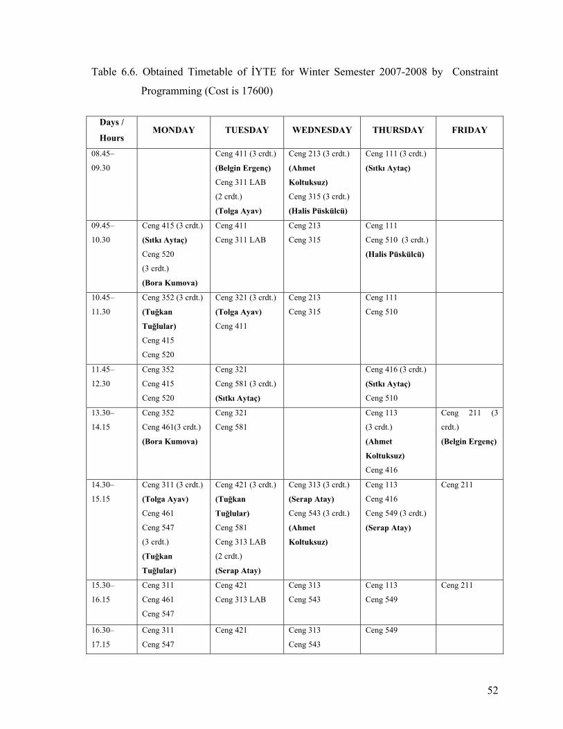
Table 6.6. Obtained Timetable of İYTE for Winter Semester 2007-2008 by Constraint

Programming (Cost is 17600)

Days /

Hours MONDAY TUESDAY WEDNESDAY THURSDAY FRIDAY

08.45–

09.30 Ceng 411 (3 crdt.)

(Belgin Ergenç)

Ceng 311 LAB

(2 crdt.)

(Tolga Ayav)

Ceng 213 (3 crdt.)

(Ahmet

Koltuksuz)

Ceng 315 (3 crdt.)

(Halis Püskülcü)

Ceng 111 (3 crdt.)

(Sıtkı Aytaç)

09.45–

10.30

Ceng 415 (3 crdt.)

(Sıtkı Aytaç)

Ceng 520

(3 crdt.)

(Bora Kumova)

Ceng 411

Ceng 311 LAB

Ceng 213

Ceng 315 Ceng 111

Ceng 510 (3 crdt.)

(Halis Püskülcü)

10.45–

11.30

Ceng 352 (3 crdt.)

(Tuğkan

Tuğlular)

Ceng 415

Ceng 520

Ceng 321 (3 crdt.)

(Tolga Ayav)

Ceng 411

Ceng 213

Ceng 315 Ceng 111

Ceng 510

11.45–

12.30

Ceng 352

Ceng 415

Ceng 520

Ceng 321

Ceng 581 (3 crdt.)

(Sıtkı Aytaç)

Ceng 416 (3 crdt.)

(Sıtkı Aytaç)

Ceng 510

13.30–

14.15

Ceng 352

Ceng 461(3 crdt.)

(Bora Kumova)

Ceng 321

Ceng 581 Ceng 113

(3 crdt.)

(Ahmet

Koltuksuz)

Ceng 416

Ceng 211 (3

crdt.)

(Belgin Ergenç)

14.30–

15.15

Ceng 311 (3 crdt.)

(Tolga Ayav)

Ceng 461

Ceng 547

(3 crdt.)

(Tuğkan

Tuğlular)

Ceng 421 (3 crdt.)

(Tuğkan

Tuğlular)

Ceng 581

Ceng 313 LAB

(2 crdt.)

(Serap Atay)

Ceng 313 (3 crdt.)

(Serap Atay)

Ceng 543 (3 crdt.)

(Ahmet

Koltuksuz)

Ceng 113

Ceng 416

Ceng 549 (3 crdt.)

(Serap Atay)

Ceng 211

15.30–

16.15

Ceng 311

Ceng 461

Ceng 547

Ceng 421

Ceng 313 LAB

Ceng 313

Ceng 543 Ceng 113

Ceng 549

Ceng 211

16.30–

17.15

Ceng 311

Ceng 547

Ceng 421 Ceng 313

Ceng 543 Ceng 549

52

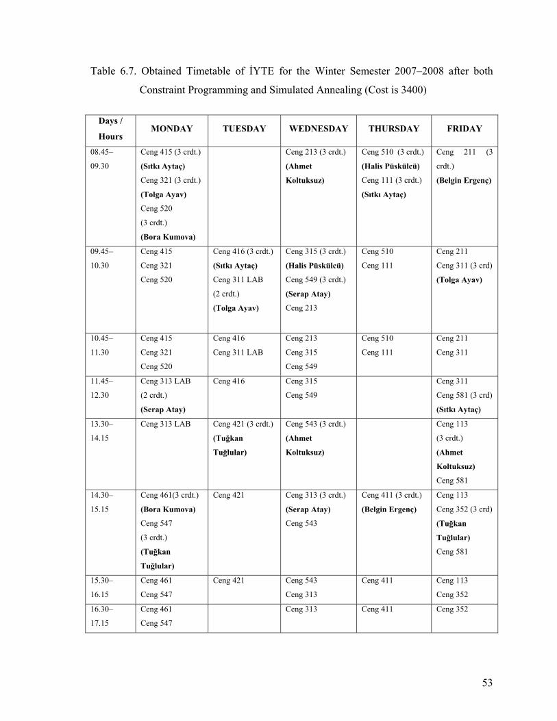
Table 6.7. Obtained Timetable of İYTE for the Winter Semester 2007–2008 after both

Constraint Programming and Simulated Annealing (Cost is 3400)

Days /

Hours MONDAY TUESDAY WEDNESDAY THURSDAY FRIDAY

08.45–

09.30

Ceng 415 (3 crdt.)

(Sıtkı Aytaç)

Ceng 321 (3 crdt.)

(Tolga Ayav)

Ceng 520

(3 crdt.)

(Bora Kumova)

Ceng 213 (3 crdt.)

(Ahmet

Koltuksuz)

Ceng 510 (3 crdt.)

(Halis Püskülcü)

Ceng 111 (3 crdt.)

(Sıtkı Aytaç)

Ceng 211 (3

crdt.)

(Belgin Ergenç)

09.45–

10.30

Ceng 415

Ceng 321

Ceng 520

Ceng 416 (3 crdt.)

(Sıtkı Aytaç)

Ceng 311 LAB

(2 crdt.)

(Tolga Ayav)

Ceng 315 (3 crdt.)

(Halis Püskülcü)

Ceng 549 (3 crdt.)

(Serap Atay)

Ceng 213

Ceng 510

Ceng 111 Ceng 211

Ceng 311 (3 crd)

(Tolga Ayav)

10.45–

11.30

Ceng 415

Ceng 321

Ceng 520

Ceng 416

Ceng 311 LAB

Ceng 213

Ceng 315 Ceng 549

Ceng 510

Ceng 111 Ceng 211

Ceng 311

11.45–

12.30

Ceng 313 LAB

(2 crdt.)

(Serap Atay)

Ceng 416

Ceng 315

Ceng 549 Ceng 311

Ceng 581 (3 crd)

(Sıtkı Aytaç)

13.30–

14.15

Ceng 313 LAB

Ceng 421 (3 crdt.)

(Tuğkan

Tuğlular)

Ceng 543 (3 crdt.)

(Ahmet

Koltuksuz)

Ceng 113

(3 crdt.)

(Ahmet

Koltuksuz)

Ceng 581

14.30–

15.15

Ceng 461(3 crdt.)

(Bora Kumova)

Ceng 547

(3 crdt.)

(Tuğkan

Tuğlular)

Ceng 421 Ceng 313 (3 crdt.)

(Serap Atay)

Ceng 543

Ceng 411 (3 crdt.)

(Belgin Ergenç)

Ceng 113

Ceng 352 (3 crd)

(Tuğkan

Tuğlular)

Ceng 581

15.30–

16.15

Ceng 461

Ceng 547

Ceng 421 Ceng 543

Ceng 313

Ceng 411 Ceng 113

Ceng 352 16.30–

17.15

Ceng 461

Ceng 547

Ceng 313 Ceng 411 Ceng 352

53

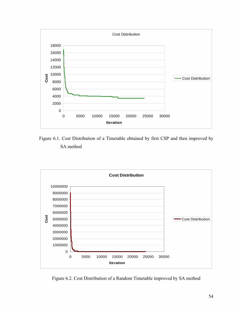
Cost Distribution

0

2000

4000

6000

8000

10000

12000

14000

16000

18000

0 5000 10000 15000 20000 25000 30000

Iteration

Cos

t

Cost Distribution

Figure 6.1. Cost Distribution of a Timetable obtained by first CSP and then improved by

SA method

Cost Distribution

0

1000000

2000000

3000000

4000000

5000000

6000000

7000000

8000000

9000000

10000000

0 5000 10000 15000 20000 25000 30000

Iteration

Cos

t

Cost Distribution

Figure 6.2. Cost Distribution of a Random Timetable improved by SA method

54

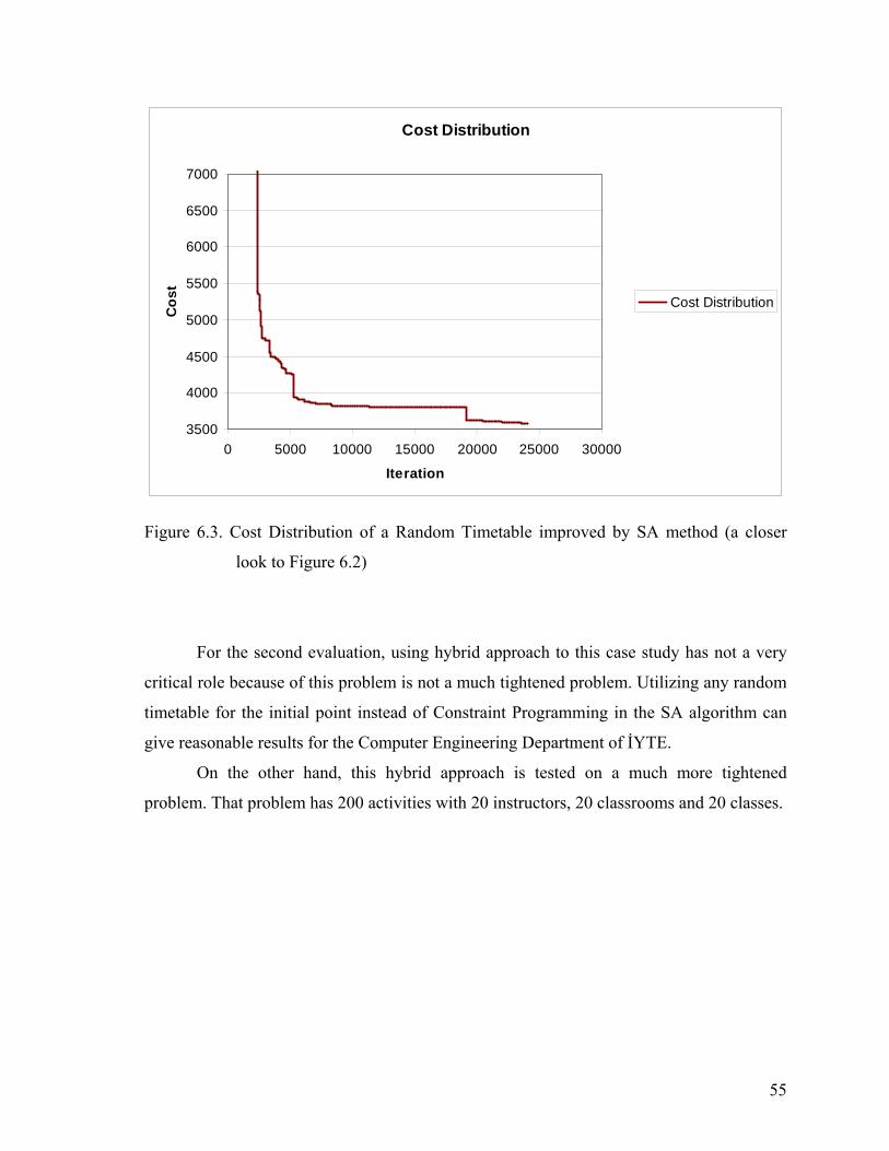
Cost Distribution

3500

4000

4500

5000

5500

6000

6500

7000

0 5000 10000 15000 20000 25000 30000

Iteration

Cos

t

Cost Distribution

Figure 6.3. Cost Distribution of a Random Timetable improved by SA method (a closer

look to Figure 6.2)

For the second evaluation, using hybrid approach to this case study has not a very

critical role because of this problem is not a much tightened problem. Utilizing any random

timetable for the initial point instead of Constraint Programming in the SA algorithm can

give reasonable results for the Computer Engineering Department of İYTE.

On the other hand, this hybrid approach is tested on a much more tightened

problem. That problem has 200 activities with 20 instructors, 20 classrooms and 20 classes.

55

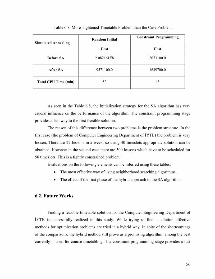
Table 6.8. More Tightened Timetable Problem than the Case Problem

Random Initial Constraint Programming Simulated Annealing

Cost Cost

Before SA 2.082161E8 2073100.0

After SA 9571100.0 1639700.0

Total CPU Time (min) 52 43

As seen in the Table 6.8, the initialization strategy for the SA algorithm has very

crucial influence on the performance of the algorithm. The constraint programming stage

provides a fast way to the first feasible solution.

The reason of this difference between two problems is the problem structure. In the

first case (the problem of Computer Engineering Department of İYTE) the problem is very

loosen. There are 22 lessons in a week, so using 40 timeslots appropriate solution can be

obtained. However in the second case there are 300 lessons which have to be scheduled for

50 timeslots. This is a tightly constrained problem.

Evaluations on the following elements can be inferred using these tables:

• The most effective way of using neighborhood searching algorithms,

• The effect of the first phase of the hybrid approach to the SA algorithm.

6.2. Future Works

Finding a feasible timetable solution for the Computer Engineering Department of

İYTE is successfully realized in this study. While trying to find a solution effective

methods for optimization problems are tried in a hybrid way. In spite of the shortcomings

of the comparisons, the hybrid method still prove as a promising algorithm, among the best

currently is used for course timetabling. The constraint programming stage provides a fast

56

way to the first feasible solution. This solution is improved by the simulated annealing

stage.

For a future work the results of the experiments demonstrated in the previous

section can be improved by some modifications in the implementation of the SA algorithm.

The stage of the hybrid approach may be integrated more fully, to yield a more powerful

and robust algorithm.

Another method for obtaining more quality results can be performing reheating

techniques in simulated annealing method in a more effective way. By reheating one can

get rid of from local minimal points and can reach to the global minimal point. Due to

performing reheating method can cause high costs for wider range of problem instances,

working on reheating worth to obtain more qualified solutions.

The other future studies about optimization problem searching methods can be

planned such as trying the hybrid two stage methods consisting of constraint programming

and tabu search for course timetabling problem, and to compare results between the two

different hybrid methods on the same data set.

57

REFERENCES

Abdennadeher, S. and M. Marte. 2000. University course timetabling using constraint

handling rules. Journal of Applied Artificial Intelligence 14(4): 311–326.

Abramson, D. 1991. Constructing school timetables using simulated annealing: Sequential

and parallel algorithms. Management Science 37(1): 98–113.

Abramson, D. and J. Abela. 1991. A parallel genetic algorithm for solving the school

timetabling problem. Technical Report, Division of Information Technology,

Commonwealth Scientific and Industrial Research Organisation.

Almond, M. 1966. An algorithm for constructing university timetables. Computer Journal

8: 331–340.

Brittan, J. N. G. and F. J. M. Farley. 1971. Collage timetable construction by computer. The

Computer Journal 14: 361–365.

Brailsford, S. C., C. N. Potts, and B. M. Smith. 1999. Constraint satisfaction problems:

Algorithms and applications. European Journal of Operational Research 119: 557–

581.

Burke, E., D. Elliman, and R. Wearre. 1994. A genetic algorithm based university

timetabling system. East-West International Conference on Computer Technologies

in Education 1: 35–40

Burke, E., J. Kingston, K. Jackson, and R. Weare. 1997. Automated university timetabling:

The state of the art. The Computer Journal 40(9): 565–571.

58

Burke, E., Y. Bykov, J. Newall, and S. Petrovic. 2001. A time-predefined local search

approach to exam timetabling problems. Computer Science Technical Report

NOTTCS-TR–2001–6, University of Nottingham.

Cérny, V. 1984. Minimization of continuous functions by simulated annealing. Technical

Report HU-TFT–84–51, Research Institute for Theoretical Physics, University of

Helsinki.

Chan, P. 2008. Constraint Satisfaction Problems. Florida Institute of Technology.

http://www.cs.fit.edu/~pkc/classes/ai/ (accessed September 28, 2008)

Cooper, T. B. and J. H. Kingston. 1996. The complexity of timetable construction

problems. In Practice and Theory of Automated Timetabling, 283–295.

Costa, D. 1994. A tabu search algorithm for computing an operational timetable. European

Journal of Operational Research 76(1): 98–110.

Deris, S., S. Omatu, H. Ohta, and P. Samat. 1997. University timetabling by constraint

based reasoning: A case study. Journal of the Operational Research Society 48:

1178–1190.

de Kleer, J. and B. C. Williams. 1986. Reasoning about multiple faults. Proceedings of

American Association for Artificial Intelligence 86: 132–139.

de Kleer, J. 1989. A comparison of ATMS and CSP techniques. Proceedings of the

Eleventh International Joint Conference on Artificial Intelligence 290–296.

Duong, T. and K. Lam. 2004. Combining constraint programming and simulated annealing

on university exam timetabling. Research Informatics Vietnam & Francophone 205–

210.

59

Feller, W. 1950. An introduction to probability theory and its applications 1. New York:

Wiley.

Freuder, E. C. 1989. Partial constraint satisfaction. International Joint Conference on

Artificial Intelligence 278–283.

Freuder, E. C. and R.J. Wallace. 1992. Partial Constraint Satisfaction. Artificial

Intelligence 58: 21–70.

Gaschnig, J. 1979. Performance measurement and analysis of certain search algorithms.

Carnegie-Mellon University thesis of PhD.

Gelfand, S. and S. Mitter. 1985. Analysis of simulated annealing for optimization. In

Proceedings of 24th Conference on Decision and Control 779–786.

German, S. and D. German. 1984. Stochastic relaxation, Gibbs distributions, and the

Bayesian restoration of images. Institute of Electrical and Electronics Engineers

Transactions of Pattern Analysis and Machine Intelligence 6: 721–741.

Gidas, B. 1984. Non-stational Markov chains and convergence of the annealing algorithm.

Journal of Statistical Physics 39: 73–131.

Guéret, C. Jussien, N. Boizumault, and P. Prins. 1996. Building university timetables using

constraint logic programming. In Practice and Theory of Automated Timetabling

130–145.

Gunadhi, H., V.J. Anand, and W.Y. Yeong. 1996. Automated timetabling using an object

oriented scheduler. Expert Systems with Applications 10(2): 243–256.

Hertz, A. 1992. Finding a feasible course schedule using tabu search. Discrete Applied

Mathematics 35: 55–270.

60

Ingber, L. 1989. Very fast simulated reannealing. Mathematical and Computer Modelling

12(8): 967–973.

Isaacson, D. L. and R. W. Madsen. 1976. Markov chains, theory and applications. New

York: Wiley.

Jaffar, J. and M. J. Maher. 1994. Constraint logic programming: A survey. The Journal of

Logic Programming 19: 503–581.

Kirkpatrick, S., C.D. Gelatt, and M.P. Vecchi. 1982. Optimization by simulated annealing.

IBM Research Report RC 9355.

Kirkpatrick, S., C.D. Gelatt, and M.P. Vecchi. 1983. Optimization by simulated annealing.

Science 4598: 671–680.

Lajos, G. 1996. Complete university modular timetabling using constraint logic

programming. In Practice and Theory of Automated Timetabling 141–161.

Lundy, M. and A. Mees. 1986. Convergence of the annealing algorithm. Mathematical

Programming 34: 111–124.

Metropolis, N., A.W. Rosenbluth, M.N. Rosenbluth, A.H. Teller, and E.Teller. 1953.

Equation of state calculations by fast computing machines. Journal of Chemical

Physics 21(6): 1087–1092.

Mitra, D., F. Romeo, and A. L. Sangiovanni-Vincentelli. 1986. Convergence and finite-

time behaviour of simulated annealing. Advanced Applied Probability 18: 747–771.

Motwani, R. and P. Raghavan. 1995. Randomized algorithms. Cambridge: Cambridge

University Press.

61

Muller, T. 2005. Constraint solver library. GNU Lesser General Public License,

SourceForge.net. http://cpsolver.sf.net (accessed December 14, 2007).

Muller, T. 2005. Constraint-based Timetabling. Charles University thesis of PhD.

Otten, R. and L. van Ginneken. 1989. The annealing algorithm. Boston/Dordrecht/London:

Kluwer Academic Publishers.

Patrick, P. 1993. Hybrid algorithms for the constraint satisfaction problem. Computational

Intelligence 9(3): 268–299.

Poupaert, E. and Y. Deville. 2000. Simulated annealing with estimated temperature.

Artificial Intelligence Communications 13: 19–26.

Romeo, F. and A. Sangiovanni-Vincentelli. 1991. A theoretical framework for simulated

annealing. Algorithmica 6(3): 302–345.

Schaerf, A. 1999. A survey of automated timetabling. Articifial Intelligence Review 13(2):

87–127.

Seneta, E. 1981. Non-negative matrices and Markov chains. New York: Springer-Verlag.

Starck, V. 1996. Implementation of Simulated Annealing optimization. Helsinki University

of Technology thesis of Master.

Szu, H. and R. Hartley. 1987. Fast simulated annealing. Physics Letters 122(3, 4): 157–162.

Terashima, M. 1998. Combinations of GAs and CSP strategies for solving the examination

timetabling problem. Instiuto Technologico y de Estudios Superiores de Monterrey

thesis of PhD.

62

Tripathy, A. 1984. School Timetabling, A Case in large binary integer linear programming.

Management Science 30: 1473–1489.

Tripathy, A. 1992. A case analysis about computerised decision aid for timetabling.

Discrete Applied Mathematics 35(3): 313–323.

Tsang, E.P.K. and T. Warwick. 1990. Applying genetic algorithms to constraint satisfaction

optimization problems. European Conference on Artificial Intelligence 649–654.

Tsang, E.P.K. 1993. Foundations of constraint satisfaction. London and San Diego,

Academic Press. http://cswww.essex.ac.uk/Research/CSP/edward/FCS.html (accessed

November 25, 2007).

Vitanyi, P. 1981. How well can a graph be n-colored. Discrete Mathematics 34: 69–80.

Werra, D. 1997. Restricted colored models for timetabling. Discrete Mathematics 165–166:

161–170.

Werra, D. 1985. An introduction to timetabling. European Journal of Operation Research

19: 151–162.

Wren, A. 1996. Scheduling, timetabling and rostering – A special relationship. In Practice

and Theory of Automated Timetabling 46–75.

Zhang, L. 2005. Solving the timetabling problem using the constraint satisfaction.

University of Wollongong thesis of Master.

63

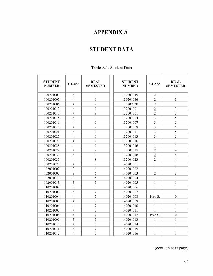
APPENDIX A

STUDENT DATA

Table A.1. Student Data

STUDENT NUMBER CLASS REAL

SEMESTER STUDENT NUMBER CLASS REAL

SEMESTER

100201003 4 9 130201045 2 3 100201005 4 9 130201046 2 3 100201006 4 9 130202020 2 3 100201012 4 9 132001001 2 3 100201013 4 9 132001001 2 3 100201015 4 9 132001004 3 5 100201016 4 9 132001007 3 5 100201018 4 9 132001009 3 5 100201021 4 9 132001011 3 5 100201025 4 9 132001013 3 5 100201027 4 9 132001016 1 1 100201028 4 9 132001016 1 1 100201029 4 9 132001017 2 4 100201030 4 9 132001018 2 4 100201035 4 8 132001023 2 4 100202025 4 7 140201001 1 1 102001007 3 6 140201002 1 1 102001007 3 6 140201003 2 3 102001013 3 5 140201004 1 1 102001013 3 5 140201005 1 1 110201002 3 5 140201006 1 1 110201003 4 7 140201007 1 1 110201004 4 7 140201008 Prep S. 0 110201005 4 7 140201009 1 1 110201006 4 7 140201010 1 1 110201007 4 7 140201011 1 1 110201008 4 7 140201012 Prep S. 0 110201009 3 5 140201013 1 1 110201010 4 7 140201014 1 3 110201011 4 7 140201015 1 1 110201012 4 7

140201016 1 1

(cont. on next page)

64

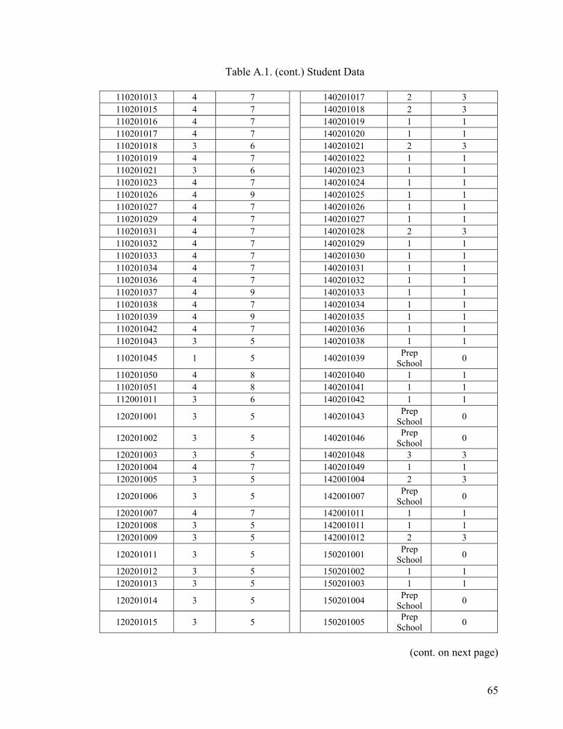
Table A.1. (cont.) Student Data

110201013 4 7 140201017 2 3 110201015 4 7 140201018 2 3 110201016 4 7 140201019 1 1 110201017 4 7 140201020 1 1 110201018 3 6 140201021 2 3 110201019 4 7 140201022 1 1 110201021 3 6 140201023 1 1 110201023 4 7 140201024 1 1 110201026 4 9 140201025 1 1 110201027 4 7 140201026 1 1 110201029 4 7 140201027 1 1 110201031 4 7 140201028 2 3 110201032 4 7 140201029 1 1 110201033 4 7 140201030 1 1 110201034 4 7 140201031 1 1 110201036 4 7 140201032 1 1 110201037 4 9 140201033 1 1 110201038 4 7 140201034 1 1 110201039 4 9 140201035 1 1 110201042 4 7 140201036 1 1 110201043 3 5 140201038 1 1

110201045 1 5 140201039 Prep School 0

110201050 4 8 140201040 1 1 110201051 4 8 140201041 1 1 112001011 3 6 140201042 1 1

120201001 3 5 140201043 Prep School 0

120201002 3 5 140201046 Prep School 0

120201003 3 5 140201048 3 3 120201004 4 7 140201049 1 1 120201005 3 5 142001004 2 3

120201006 3 5 142001007 Prep School 0

120201007 4 7 142001011 1 1 120201008 3 5 142001011 1 1 120201009 3 5 142001012 2 3

120201011 3 5 150201001 Prep School 0

120201012 3 5 150201002 1 1 120201013 3 5 150201003 1 1

120201014 3 5 150201004 Prep School 0

120201015 3 5

150201005 Prep School 0

(cont. on next page)

65

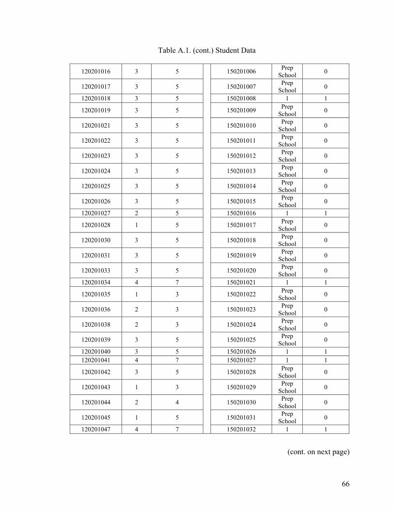
Table A.1. (cont.) Student Data

120201016 3 5 150201006 Prep School 0

120201017 3 5 150201007 Prep School 0

120201018 3 5 150201008 1 1

120201019 3 5 150201009 Prep School 0

120201021 3 5 150201010 Prep School 0

120201022 3 5 150201011 Prep School 0

120201023 3 5 150201012 Prep School 0

120201024 3 5 150201013 Prep School 0

120201025 3 5 150201014 Prep School 0

120201026 3 5 150201015 Prep School 0

120201027 2 5 150201016 1 1

120201028 1 5 150201017 Prep School 0

120201030 3 5 150201018 Prep School 0

120201031 3 5 150201019 Prep School 0

120201033 3 5 150201020 Prep School 0

120201034 4 7 150201021 1 1

120201035 1 3 150201022 Prep School 0

120201036 2 3 150201023 Prep School 0

120201038 2 3 150201024 Prep School 0

120201039 3 5 150201025 Prep School 0

120201040 3 5 150201026 1 1 120201041 4 7 150201027 1 1

120201042 3 5 150201028 Prep School 0

120201043 1 3 150201029 Prep School 0

120201044 2 4 150201030 Prep School 0

120201045 1 5 150201031 Prep School 0

120201047 4 7

150201032 1 1

(cont. on next page)

66

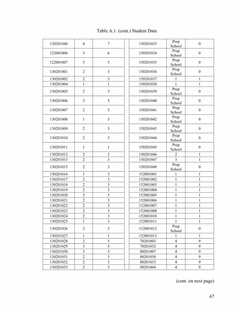
Table A.1. (cont.) Student Data

120201048 4 7 150201033 Prep School 0

122001006 3 6 150201034 Prep School 0

122001007 3 5 150201035 Prep School 0

130201001 2 3 150201036 Prep School 0

130201002 2 3 150201037 1 1 130201004 1 1 150201038 1 1

130201005 2 3 150201039 Prep School 0

150201040 Prep School 0 130201006 3 5

150201041 Prep School 0 130201007 2 5

150201042 Prep School 130201008 1 3 0

130201009 2 3 150201043 Prep School 0

130201010 2 3 150201044 Prep School 0

130201011 1 1 150201045 Prep School 0

130201012 2 3 150201046 2 1 130201013 2 3 150201047 3 1

130201015 2 3 150201049 Prep School 0

130201016 1 3 152001001 1 1 130201017 2 3 152001002 1 1 130201018 2 3 152001003 1 1 130201019 2 3 152001004 1 1 130201020 2 3 152001005 1 1 130201021 2 3 152001006 1 1 130201022 2 3 152001007 1 1 130201023 2 3 152001008 1 1 130201024 2 3 152001010 1 1 130201025 1 3 152001011 1 1

130201026 2 3 152001012 Prep School 0

130201027 1 1 152001013 1 1 130201028 2 5 70201003 4 9 130201029 3 5 70201032 4 9 130201030 3 5 80201007 4 9 130201031 2 3 80201030 4 9 130201032 2 3

80201033 4 9 130201033 2 3 90201004 4 9

(cont. on next page)

67

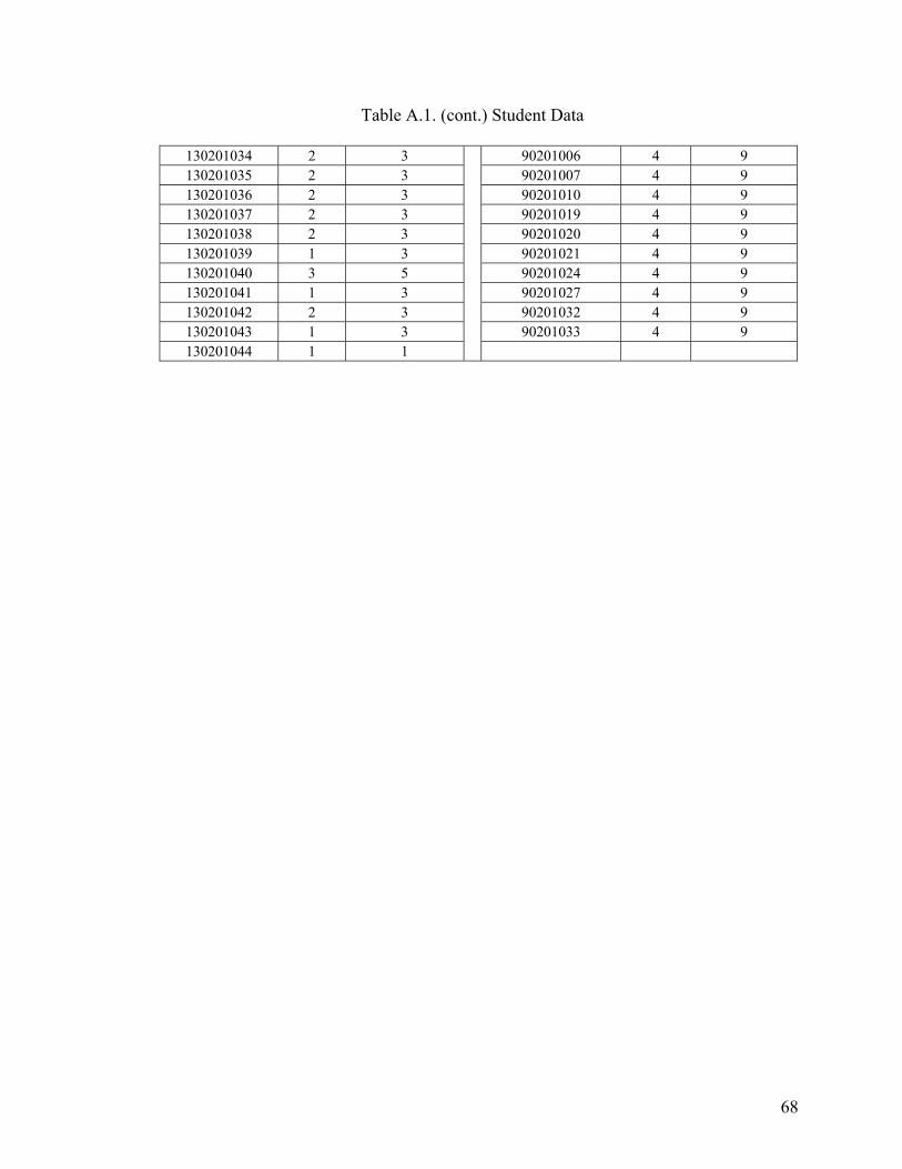
Table A.1. (cont.) Student Data

130201034 2 3 90201006 4 9 130201035 2 3 90201007 4 9 130201036 2 3 90201010 4 9 130201037 2 3 90201019 4 9 130201038 2 3 90201020 4 9 130201039 1 3 90201021 4 9 130201040 3 5 90201024 4 9 130201041 1 3 90201027 4 9 130201042 2 3 90201032 4 9 130201043 1 3 90201033 4 9 130201044 1 1

68

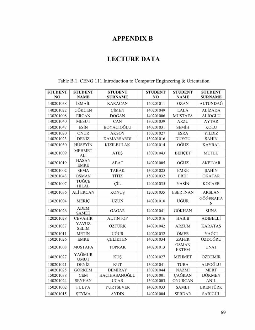
APPENDIX B

LECTURE DATA

Table B.1. CENG 111 Introduction to Computer Engineering & Orientation

STUDENT NO

STUDENT NAME

STUDENT SURNAME STUDENT

NO STUDENT

NAME STUDENT SURNAME

140201038 İSMAİL KARACAN 140201011 OZAN ALTUNDAĞ 140201022 GÖKÇEN ÇİMEN 140201049 LALA ALİZADA 130201008 ERCAN DOĞAN 140201006 MUSTAFA ALİOĞLU 140201040 MESUT CAN 130201039 ARZU AYTAR 150201047 ESİN BOYACIOĞLU 140201031 SEMİH KOLU 140201020 ONUR AKSOY 150201027 ESRA YILDIZ 140201023 DENİZ DAMARSARDI 150201016 DUYGU ŞAHİN 140201030 HÜSEYİN KIZILBULAK 140201014 OĞUZ KAYRAL

140201009 MEHMET ALİ ATEŞ 130201043 BEHÇET MUTLU

140201019 HASAN EMRE ABAT 140201005 OĞUZ AKPINAR

140201002 SEMA TABAK 130201025 EMRE ŞAHİN 120201043 OSMAN TİTİZ 150201032 ERDİ OKATAR

140201007 TUĞÇE HİLAL ÇİL 140201035 YASİN KOCAER

140201036 ALİ ERCAN KONUŞ 120201035 ESER İNAN ARSLAN

130201004 MERİÇ UZUN 140201010 UĞUR GÖĞEBAKAN

140201026 ADEM SAMET GAGAR 140201041 GÖKHAN SUNA

120201028 CEVAHİR ALTINTOP 140201016 HABİB ADIBELLİ

150201037 YAVUZ SELİM ÖZTÜRK 140201042 ARZUM KARATAŞ

130201011 METİN UĞUR 140201032 ÖMER YAĞCI 150201026 EMRE ÇELİKTEN 140201034 ZAFER ÖZDOĞRU

150201008 MUSTAFA TOPRAK 140201013 OSMAN ERTEM UNAT

140201027 YAĞMUR UMUT KUŞ 130201027 MEHMET ÖZDEMİR

150201021 DENİZ KUT 130201041 TUBA ALPOĞLU 140201025 GÖRKEM DEMİRAY 130201044 NAZMİ MERT 150201038 CEM HACIHASANOĞLU 140201001 ÇAĞKAN DÖKMEN 140201024 SEYHAN UÇAR 150201003 ONURCAN ANIL 150201002 FULYA YURTSEVER 140201033 SAMET ERENTÜRK 140201015 ŞEYMA AYDIN 140201004 SERDAR SARIGÜL

69

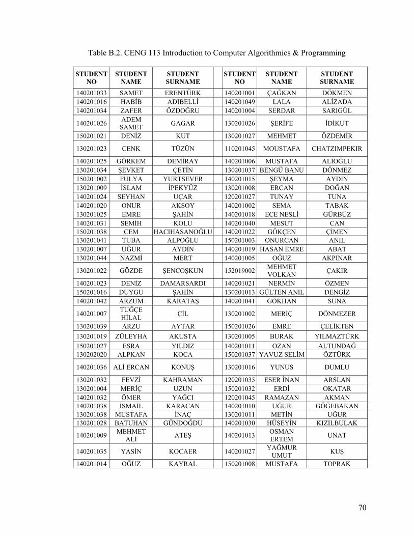
Table B.2. CENG 113 Introduction to Computer Algorithmics & Programming

STUDENT NO

STUDENT NAME

STUDENT SURNAME STUDENT

NO STUDENT

NAME STUDENT SURNAME

140201033 SAMET ERENTÜRK 140201001 ÇAĞKAN DÖKMEN 140201016 HABİB ADIBELLİ 140201049 LALA ALİZADA 140201034 ZAFER ÖZDOĞRU 140201004 SERDAR SARIGÜL

140201026 ADEM SAMET GAGAR 130201026 ŞERİFE İDİKUT

150201021 DENİZ KUT 130201027 MEHMET ÖZDEMİR

130201023 CENK TÜZÜN 110201045 MOUSTAFA CHATZIMPEKIR

140201025 GÖRKEM DEMİRAY 140201006 MUSTAFA ALİOĞLU 130201034 ŞEVKET ÇETİN 130201037 BENGÜ BANU DÖNMEZ 150201002 FULYA YURTSEVER 140201015 ŞEYMA AYDIN 130201009 İSLAM İPEKYÜZ 130201008 ERCAN DOĞAN 140201024 SEYHAN UÇAR 120201027 TUNAY TUNA 140201020 ONUR AKSOY 140201002 SEMA TABAK 130201025 EMRE ŞAHİN 140201018 ECE NESLİ GÜRBÜZ 140201031 SEMİH KOLU 140201040 MESUT CAN 150201038 CEM HACIHASANOĞLU 140201022 GÖKÇEN ÇİMEN 130201041 TUBA ALPOĞLU 150201003 ONURCAN ANIL 130201007 UĞUR AYDIN 140201019 HASAN EMRE ABAT 130201044 NAZMİ MERT 140201005 OĞUZ AKPINAR

130201022 GÖZDE ŞENCOŞKUN 152019002 MEHMET VOLKAN ÇAKIR

140201023 DENİZ DAMARSARDI 140201021 NERMİN ÖZMEN 150201016 DUYGU ŞAHİN 130201013 GÜLTEN ANIL DENGİZ 140201042 ARZUM KARATAŞ 140201041 GÖKHAN SUNA

140201007 TUĞÇE HİLAL ÇİL 130201002 MERİÇ DÖNMEZER

130201039 ARZU AYTAR 150201026 EMRE ÇELİKTEN 130201019 ZÜLEYHA AKUSTA 130201005 BURAK YILMAZTÜRK 150201027 ESRA YILDIZ 140201011 OZAN ALTUNDAĞ 130202020 ALPKAN KOCA 150201037 YAVUZ SELİM ÖZTÜRK

140201036 ALİ ERCAN KONUŞ 130201016 YUNUS DUMLU

130201032 FEVZİ KAHRAMAN 120201035 ESER İNAN ARSLAN 130201004 MERİÇ UZUN 150201032 ERDİ OKATAR 140201032 ÖMER YAĞCI 120201045 RAMAZAN AKMAN 140201038 İSMAİL KARACAN 140201010 UĞUR GÖĞEBAKAN 130201038 MUSTAFA İNAÇ 130201011 METİN UĞUR 130201028 BATUHAN GÜNDOĞDU 140201030 HÜSEYİN KIZILBULAK

140201009 MEHMET ALİ ATEŞ 140201013 OSMAN

ERTEM UNAT

140201035 YASİN KOCAER 140201027 YAĞMUR UMUT KUŞ

140201014 OĞUZ KAYRAL 150201008 MUSTAFA TOPRAK

70

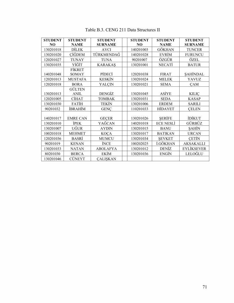
Table B.3. CENG 211 Data Structures II

STUDENT NO

STUDENT NAME

STUDENT SURNAME STUDENT

NO STUDENT

NAME STUDENT SURNAME

130201018 DİLEK AVCI 140201003 GÖKHAN TUNCER 130201020 ÇİĞDEM TÜRKMENDAĞ 140201028 EVRİM FURUNCU 120201027 TUNAY TUNA 90201007 ÖZGÜR ÖZEL 130201035 YİĞİT KARAKAŞ 130201001 NECATİ BATUR

140201048 FİKRET SOMAY PİDECİ 120201038 FIRAT ŞAHİNDAL

120201013 MUSTAFA KESKİN 130201024 MELEK YAVUZ 120201018 BORA YALÇIN 130201021 SEMA ÇAM

130201013 GÜLTEN

ANIL DENGİZ 130201045 ASİYE KILIÇ 120201005 CİHAT TOMBAK 130201031 SEDA KASAP 130201030 FATİH TEKİN 130201006 ERDEM SARILI 90201032 İBRAHİM GENÇ 110201033 HİDAYET ÇELEN

140201017 EMRE CAN GEÇER 130201026 ŞERİFE İDİKUT 130201010 İPEK YAĞCAN 140201018 ECE NESLİ GÜRBÜZ 130201007 UĞUR AYDIN 130201015 BANU ŞAHİN 100201018 MEHMET KOÇA 130201017 BATIKAN URCAN 120201036 BASRİ MUMCU 130201034 ŞEVKET ÇETİN 90201019 KENAN İNCE 100202025 İ.GÖKHAN AKSAKALLI

130201033 NATAN ABOLAFYA 130201012 DENİZ EYLİKSEVER 80201030 BERCA EKİM 130201036 ENGİN LELOĞLU

130201046 CÜNEYT ÇALIŞKAN

71

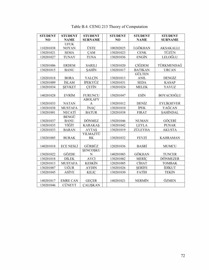
Table B.4. CENG 213 Theory of Computation

STUDENT NO

STUDENT NAME

STUDENT SURNAME STUDENT

NO STUDENT

NAME STUDENT SURNAME

110201038 UFUK

NOYAN ÜSTE 100202025 İ.GÖKHAN AKSAKALLI 130201021 SEMA ÇAM 130201023 CENK TÜZÜN 120201027 TUNAY TUNA 130201036 ENGİN LELOĞLU

130201006 ERDEM SARILI 130201020 ÇİĞDEM TÜRKMENDAĞ 130201015 BANU ŞAHİN 130201017 BATIKAN URCAN

120201018 BORA YALÇIN 130201013 GÜLTEN

ANIL DENGİZ 130201009 İSLAM İPEKYÜZ 130201031 SEDA KASAP 130201034 ŞEVKET ÇETİN 130201024 MELEK YAVUZ

140201028 EVRİM FURUNCU 150201047 ESİN BOYACIOĞLU

130201033 NATAN ABOLAFY

A 130201012 DENİZ EYLİKSEVER 130201038 MUSTAFA İNAÇ 130201010 İPEK YAĞCAN 130201001 NECATİ BATUR 120201038 FIRAT ŞAHİNDAL

130201037 BENGÜ BANU DÖNMEZ 150201046 NUMAN GÖÇERİ

130201035 YİĞİT KARAKAŞ 130201042 LEYLA PUNAR 120201033 BARAN AYTAŞ 130201019 ZÜLEYHA AKUSTA

130201005 BURAK YILMAZTÜ

RK 130201032 FEVZİ KAHRAMAN

140201018 ECE NESLİ GÜRBÜZ 120201036 BASRİ MUMCU

130201022 GÖZDE ŞENCOŞKU

N 140201003 GÖKHAN TUNCER 130201018 DİLEK AVCI 130201002 MERİÇ DÖNMEZER 120201013 MUSTAFA KESKİN 120201005 CİHAT TOMBAK 130201007 UĞUR AYDIN 130201026 ŞERİFE İDİKUT 130201045 ASİYE KILIÇ 130201030 FATİH TEKİN

140201017 EMRE CAN GEÇER 140201021 NERMİN ÖZMEN 130201046 CÜNEYT ÇALIŞKAN

72

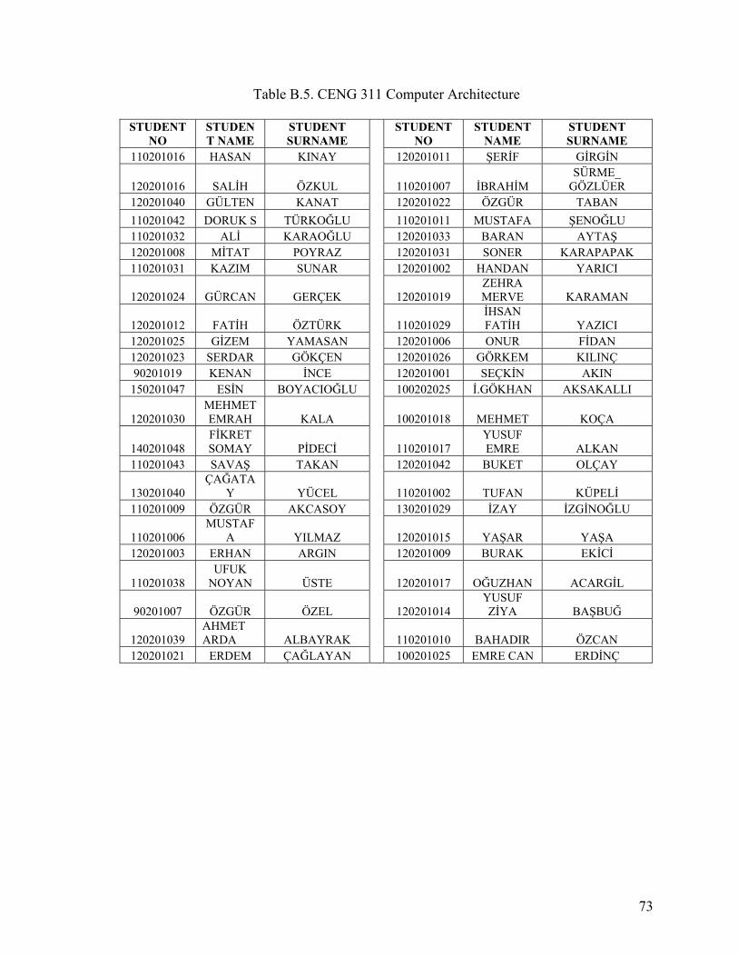
Table B.5. CENG 311 Computer Architecture

STUDENT NO

STUDENT NAME

STUDENT SURNAME

STUDENT NO

STUDENT NAME

STUDENT SURNAME

110201016 HASAN KINAY 120201011 ŞERİF GİRGİN

120201016 SALİH ÖZKUL 110201007 İBRAHİM SÜRME_

GÖZLÜER 120201040 GÜLTEN KANAT 120201022 ÖZGÜR TABAN 110201042 DORUK S TÜRKOĞLU 110201011 MUSTAFA ŞENOĞLU 110201032 ALİ KARAOĞLU 120201033 BARAN AYTAŞ 120201008 MİTAT POYRAZ 120201031 SONER KARAPAPAK 110201031 KAZIM SUNAR 120201002 HANDAN YARICI

120201024 GÜRCAN GERÇEK 120201019 ZEHRA MERVE KARAMAN

120201012 FATİH ÖZTÜRK 110201029 İHSAN FATİH YAZICI

120201025 GİZEM YAMASAN 120201006 ONUR FİDAN 120201023 SERDAR GÖKÇEN 120201026 GÖRKEM KILINÇ 90201019 KENAN İNCE 120201001 SEÇKİN AKIN 150201047 ESİN BOYACIOĞLU 100202025 İ.GÖKHAN AKSAKALLI

120201030 MEHMET EMRAH KALA 100201018 MEHMET KOÇA

140201048 FİKRET SOMAY PİDECİ 110201017

YUSUF EMRE ALKAN

110201043 SAVAŞ TAKAN 120201042 BUKET OLÇAY

130201040 ÇAĞATA

Y YÜCEL 110201002 TUFAN KÜPELİ 110201009 ÖZGÜR AKCASOY 130201029 İZAY İZGİNOĞLU

110201006 MUSTAF

A YILMAZ 120201015 YAŞAR YAŞA 120201003 ERHAN ARGIN 120201009 BURAK EKİCİ

110201038 UFUK

NOYAN ÜSTE 120201017 OĞUZHAN ACARGİL

90201007 ÖZGÜR ÖZEL 120201014 YUSUF ZİYA BAŞBUĞ

120201039 AHMET ARDA ALBAYRAK 110201010 BAHADIR ÖZCAN

120201021 ERDEM ÇAĞLAYAN

100201025 EMRE CAN ERDİNÇ

73

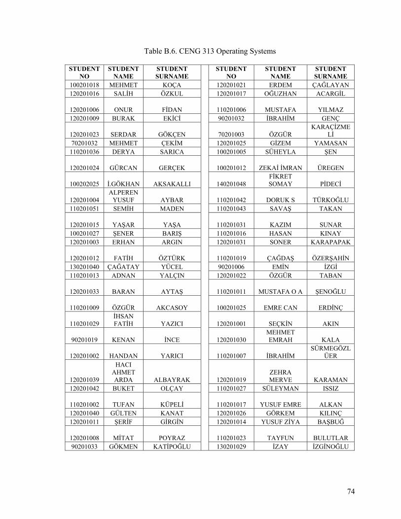
Table B.6. CENG 313 Operating Systems

STUDENT NO

STUDENT NAME

STUDENT SURNAME

STUDENT NO

STUDENT NAME

STUDENT SURNAME

100201018 MEHMET KOÇA 120201021 ERDEM ÇAĞLAYAN 120201016 SALİH ÖZKUL 120201017 OĞUZHAN ACARGİL

120201006 ONUR FİDAN 110201006 MUSTAFA YILMAZ 120201009 BURAK EKİCİ 90201032 İBRAHİM GENÇ

120201023 SERDAR GÖKÇEN 70201003 ÖZGÜR KARAÇİZME

Lİ 70201032 MEHMET ÇEKİM 120201025 GİZEM YAMASAN

110201036 DERYA SARICA 100201005 SÜHEYLA ŞEN

120201024 GÜRCAN GERÇEK 100201012 ZEKAİ İMRAN ÜREGEN

100202025 İ.GÖKHAN AKSAKALLI 140201048 FİKRET SOMAY PİDECİ

120201004 ALPEREN

YUSUF AYBAR 110201042 DORUK S TÜRKOĞLU 110201051 SEMİH MADEN 110201043 SAVAŞ TAKAN

120201015 YAŞAR YAŞA 110201031 KAZIM SUNAR 100201027 ŞENER BARIŞ 110201016 HASAN KINAY 120201003 ERHAN ARGIN 120201031 SONER KARAPAPAK

120201012 FATİH ÖZTÜRK 110201019 ÇAĞDAŞ ÖZERŞAHİN 130201040 ÇAĞATAY YÜCEL 90201006 EMİN İZGİ 110201013 ADNAN YALÇIN 120201022 ÖZGÜR TABAN

120201033 BARAN AYTAŞ 110201011 MUSTAFA O A ŞENOĞLU

110201009 ÖZGÜR AKCASOY 100201025 EMRE CAN ERDİNÇ

110201029 İHSAN FATİH YAZICI 120201001 SEÇKİN AKIN

90201019 KENAN İNCE 120201030 MEHMET EMRAH KALA

120201002 HANDAN YARICI 110201007 İBRAHİM SÜRMEGÖZL

ÜER

120201039

HACI AHMET ARDA ALBAYRAK 120201019

ZEHRA MERVE KARAMAN

120201042 BUKET OLÇAY 110201027 SÜLEYMAN ISSIZ

110201002 TUFAN KÜPELİ 110201017 YUSUF EMRE ALKAN 120201040 GÜLTEN KANAT 120201026 GÖRKEM KILINÇ 120201011 ŞERİF GİRGİN 120201014 YUSUF ZİYA BAŞBUĞ

120201008 MİTAT POYRAZ 110201023 TAYFUN BULUTLAR 90201033 GÖKMEN KATİPOĞLU

130201029 İZAY İZGİNOĞLU

74

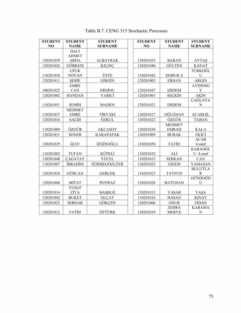
Table B.7. CENG 315 Stochastic Processes

STUDENT NO

STUDENT NAME

STUDENT SURNAME

STUDENT NO

STUDENT NAME

STUDENT SURNAME

120201039

HACI AHMET ARDA ALBAYRAK 120201033 BARAN AYTAŞ

120201026 GÖRKEM KILINÇ 120201040 GÜLTEN KANAT

110201038 UFUK

NOYAN ÜSTE 110201042 DORUK S TÜRKOĞL

U 120201011 ŞERİF GİRGİN 120201003 ERHAN ARGIN

100201025 EMRE CAN ERDİNÇ 120201047 ERDEM

AYDINSOY

120201002 HANDAN YARICI 120201001 SEÇKİN AKIN

110201051 SEMİH MADEN 120201021 ERDEM ÇAĞLAYA

N

110201037 MEHMET

EMRE TİRYAKİ 120201017 OĞUZHAN ACARGİL 120201016 SALİH ÖZKUL 120201022 ÖZGÜR TABAN

110201009 ÖZGÜR AKCASOY 120201030 MEHMET EMRAH KALA

120201031 SONER KARAPAPAK 120201009 BURAK EKİCİ

130201029 İZAY İZGİNOĞLU 110201050 FATİH ACAR 4.sınıf

110201002 TUFAN KÜPELİ 110201032 ALİ KARAOĞL

U 4.sınıf 130201040 ÇAĞATAY YÜCEL 110201015 SERKAN CAN 110201007 İBRAHİM SÜRMEGÖZLÜER 120201025 GİZEM YAMASAN

120201024 GÜRCAN GERÇEK 110201023 TAYFUN BULUTLA

R

120201008 MİTAT POYRAZ 130201028 BATUHAN GÜNDOĞD

U

120201014 YUSUF ZİYA BAŞBUĞ 120201015 YAŞAR YAŞA

120201042 BUKET OLÇAY 110201016 HASAN KINAY 120201023 SERDAR GÖKÇEN 120201006 ONUR FİDAN

120201012 FATİH ÖZTÜRK

120201019 ZEHRA MERVE

KARAMAN

75

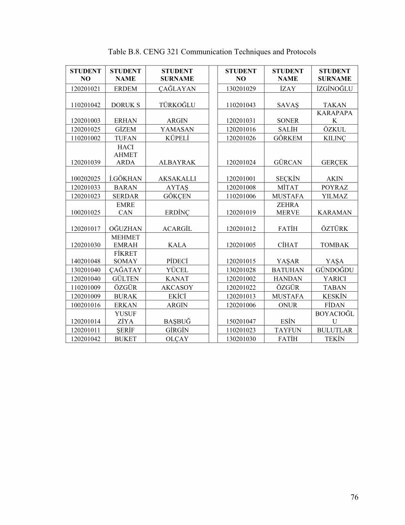
Table B.8. CENG 321 Communication Techniques and Protocols

STUDENT NO

STUDENT NAME

STUDENT SURNAME

STUDENT NO

STUDENT NAME

STUDENT SURNAME

120201021 ERDEM ÇAĞLAYAN 130201029 İZAY İZGİNOĞLU

110201042 DORUK S TÜRKOĞLU 110201043 SAVAŞ TAKAN

120201003 ERHAN ARGIN 120201031 SONER KARAPAPA

K 120201025 GİZEM YAMASAN 120201016 SALİH ÖZKUL 110201002 TUFAN KÜPELİ 120201026 GÖRKEM KILINÇ

120201039

HACI AHMET ARDA ALBAYRAK 120201024 GÜRCAN GERÇEK

100202025 İ.GÖKHAN AKSAKALLI 120201001 SEÇKİN AKIN 120201033 BARAN AYTAŞ 120201008 MİTAT POYRAZ 120201023 SERDAR GÖKÇEN 110201006 MUSTAFA YILMAZ

100201025 EMRE CAN ERDİNÇ 120201019

ZEHRA MERVE KARAMAN

120201017 OĞUZHAN ACARGİL 120201012 FATİH ÖZTÜRK

120201030 MEHMET EMRAH KALA 120201005 CİHAT TOMBAK

140201048 FİKRET SOMAY PİDECİ 120201015 YAŞAR YAŞA

130201040 ÇAĞATAY YÜCEL 130201028 BATUHAN GÜNDOĞDU 120201040 GÜLTEN KANAT 120201002 HANDAN YARICI 110201009 ÖZGÜR AKCASOY 120201022 ÖZGÜR TABAN 120201009 BURAK EKİCİ 120201013 MUSTAFA KESKİN 100201016 ERKAN ARGIN 120201006 ONUR FİDAN

120201014 YUSUF ZİYA BAŞBUĞ 150201047 ESİN

BOYACIOĞLU

120201011 ŞERİF GİRGİN 110201023 TAYFUN BULUTLAR 120201042 BUKET OLÇAY

130201030 FATİH TEKİN

76

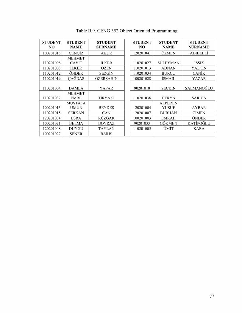
Table B.9. CENG 352 Object Oriented Programming

STUDENT NO

STUDENT NAME

STUDENT SURNAME

STUDENT NO

STUDENT NAME

STUDENT SURNAME

100201015 CENGİZ AKUR 120201041 ÖZMEN ADIBELLİ

110201008 MEHMET

CAVİT İLKER 110201027 SÜLEYMAN ISSIZ 110201003 İLKER ÖZEN 110201013 ADNAN YALÇIN 110201012 ÖNDER SEZGİN 110201034 BURCU CANİK 110201019 ÇAĞDAŞ ÖZERŞAHİN 100201028 İSMAİL YAZAR

110201004 DAMLA YAPAR 90201010 SEÇKİN SALMANOĞLU

110201037 MEHMET

EMRE TİRYAKİ 110201036 DERYA SARICA

100201013 MUSTAFA

UMUR BEYDEŞ 120201004 ALPEREN

YUSUF AYBAR 110201015 SERKAN CAN 120201007 BURHAN ÇİMEN 120201034 ESRA RÜZGAR 100201003 EMRAH ÖNDER 100201021 BELMA BOYRAZ 90201033 GÖKMEN KATİPOĞLU 120201048 DUYGU TAYLAN 110201005 ÜMİT KARA 100201027 ŞENER BARIŞ

77

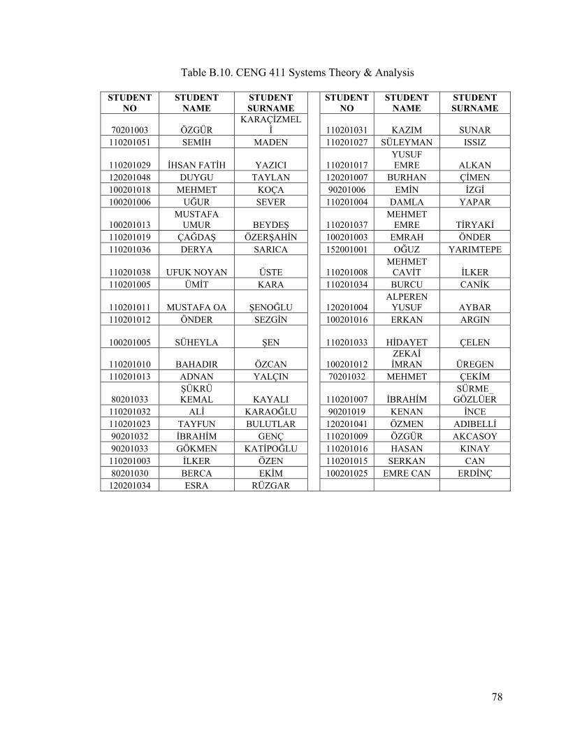
Table B.10. CENG 411 Systems Theory & Analysis

STUDENT NO

STUDENT NAME

STUDENT SURNAME

STUDENT NO

STUDENT NAME

STUDENT SURNAME

70201003 ÖZGÜR KARAÇİZMEL

İ 110201031 KAZIM SUNAR 110201051 SEMİH MADEN 110201027 SÜLEYMAN ISSIZ

110201029 İHSAN FATİH YAZICI 110201017 YUSUF EMRE ALKAN

120201048 DUYGU TAYLAN 120201007 BURHAN ÇİMEN 100201018 MEHMET KOÇA 90201006 EMİN İZGİ 100201006 UĞUR SEVER 110201004 DAMLA YAPAR

100201013 MUSTAFA

UMUR BEYDEŞ 110201037 MEHMET

EMRE TİRYAKİ 110201019 ÇAĞDAŞ ÖZERŞAHİN 100201003 EMRAH ÖNDER 110201036 DERYA SARICA 152001001 OĞUZ YARIMTEPE

110201038 UFUK NOYAN ÜSTE 110201008 MEHMET

CAVİT İLKER 110201005 ÜMİT KARA 110201034 BURCU CANİK

110201011 MUSTAFA OA ŞENOĞLU 120201004 ALPEREN

YUSUF AYBAR 110201012 ÖNDER SEZGİN 100201016 ERKAN ARGIN

100201005 SÜHEYLA ŞEN 110201033 HİDAYET ÇELEN

110201010 BAHADIR ÖZCAN 100201012 ZEKAİ İMRAN ÜREGEN

110201013 ADNAN YALÇIN 70201032 MEHMET ÇEKİM

80201033 ŞÜKRÜ KEMAL KAYALI 110201007 İBRAHİM

SÜRME_ GÖZLÜER

110201032 ALİ KARAOĞLU 90201019 KENAN İNCE 110201023 TAYFUN BULUTLAR 120201041 ÖZMEN ADIBELLİ 90201032 İBRAHİM GENÇ 110201009 ÖZGÜR AKCASOY 90201033 GÖKMEN KATİPOĞLU 110201016 HASAN KINAY

110201003 İLKER ÖZEN 110201015 SERKAN CAN 80201030 BERCA EKİM 100201025 EMRE CAN ERDİNÇ

120201034 ESRA RÜZGAR

78

Table B.11. CENG 415 Senior Design Project & Seminar I

STUDENT NO

STUDENT NAME

STUDENT SURNAME

STUDENT NO

STUDENT NAME

STUDENT SURNAME

90201020 BEKİR AHMETOĞLU 80201033 ŞÜKRÜ KEMAL KAYALI

100201003 EMRAH ÖNDER 110201019 ÇAĞDAŞ ÖZERŞAHİN 100201006 UĞUR SEVER 110201003 İLKER ÖZEN 120201041 ÖZMEN ADIBELLİ 110201005 ÜMİT KARA 110201050 FATİH ACAR 100201028 İSMAİL YAZAR 80201030 BERCA EKİM 110201051 SEMİH MADEN

110201011 MUSTAFA O A ŞENOĞLU 110201008 MEHMET

CAVİT İLKER

90201027 CEREN TEKİN 110201038 UFUK

NOYAN ÜSTE 100201029 NİGAR KALE 100201016 ERKAN ARGIN

110201037 MEHMET

EMRE TİRYAKİ 100201030 ÜMRAN KAMAR 110201004 DAMLA YAPAR 110201032 ALİ KARAOĞLU

110201026 GÖKHAN ADIGÜZEL 90201010 SEÇKİN SALMA_ NOĞLU

110201036 DERYA SARICA 110201012 ÖNDER SEZGİN

100201013 MUSTAFA

UMUR BEYDEŞ 110201013 ADNAN YALÇIN 120201007 BURHAN ÇİMEN 120201034 ESRA RÜZGAR 110201010 BAHADIR ÖZCAN 110201015 SERKAN CAN

110201034 BURCU CANİK 100201012 ZEKAİ İMRAN ÜREGEN

110201027 SÜLEYMAN ISSIZ 90201033 GÖKMEN KATİPOĞ_

LU

120201048 DUYGU TAYLAN 120201004 ALPEREN

YUSUF AYBAR

100201005 SÜHEYLA ŞEN

70201032 MEHMET ÇEKİM

Table B.12. CENG 416 Senior Design Project & Seminar II

STUDENT NO

STUDENT NAME

STUDENT SURNAME

STUDENT NO

STUDENT NAME

STUDENT SURNAME

80201007 ARİF AKYOL 100201006 UĞUR SEVER

80201033 ŞÜKRÜ KEMAL KAYALI 90201020 BEKİR AHMETOĞLU

120201047 ERDEM AYDINSOY

90201010 SEÇKİN SALMANOĞ_

LU

79

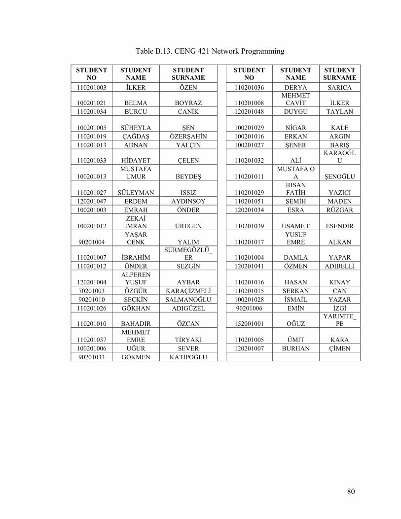
Table B.13. CENG 421 Network Programming

STUDENT NO

STUDENT NAME

STUDENT SURNAME

STUDENT NO

STUDENT NAME

STUDENT SURNAME

110201003 İLKER ÖZEN 110201036 DERYA SARICA

100201021 BELMA BOYRAZ 110201008 MEHMET

CAVİT İLKER 110201034 BURCU CANİK 120201048 DUYGU TAYLAN

100201005 SÜHEYLA ŞEN 100201029 NİGAR KALE 110201019 ÇAĞDAŞ ÖZERŞAHİN 100201016 ERKAN ARGIN 110201013 ADNAN YALÇIN 100201027 ŞENER BARIŞ

110201033 HİDAYET ÇELEN 110201032 ALİ KARAOĞL

U

100201013 MUSTAFA

UMUR BEYDEŞ 110201011 MUSTAFA O

A ŞENOĞLU

110201027 SÜLEYMAN ISSIZ 110201029 İHSAN FATİH YAZICI

120201047 ERDEM AYDINSOY 110201051 SEMİH MADEN 100201003 EMRAH ÖNDER 120201034 ESRA RÜZGAR

100201012 ZEKAİ İMRAN ÜREGEN 110201039 ÜSAME F ESENDİR

90201004 YAŞAR CENK YALIM 110201017

YUSUF EMRE ALKAN

110201007 İBRAHİM SÜRMEGÖZLÜ_

ER 110201004 DAMLA YAPAR 110201012 ÖNDER SEZGİN 120201041 ÖZMEN ADIBELLİ

120201004 ALPEREN

YUSUF AYBAR 110201016 HASAN KINAY 70201003 ÖZGÜR KARAÇİZMELİ 110201015 SERKAN CAN 90201010 SEÇKİN SALMANOĞLU 100201028 İSMAİL YAZAR

110201026 GÖKHAN ADIGÜZEL 90201006 EMİN İZGİ

110201010 BAHADIR ÖZCAN 152001001 OĞUZ YARIMTE_

PE

110201037 MEHMET

EMRE TİRYAKİ 110201005 ÜMİT KARA 100201006 UĞUR SEVER 120201007 BURHAN ÇİMEN 90201033 GÖKMEN KATİPOĞLU

80

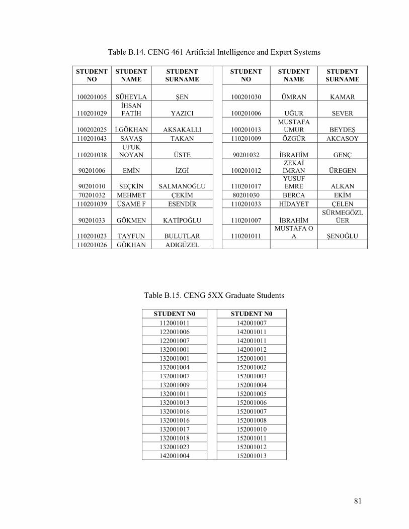
Table B.14. CENG 461 Artificial Intelligence and Expert Systems

STUDENT NO

STUDENT NAME

STUDENT SURNAME

STUDENT NO

STUDENT NAME

STUDENT SURNAME

100201005 SÜHEYLA ŞEN 100201030 ÜMRAN KAMAR

110201029 İHSAN FATİH YAZICI 100201006 UĞUR SEVER

100202025 İ.GÖKHAN AKSAKALLI 100201013 MUSTAFA

UMUR BEYDEŞ 110201043 SAVAŞ TAKAN 110201009 ÖZGÜR AKCASOY

110201038 UFUK

NOYAN ÜSTE 90201032 İBRAHİM GENÇ

90201006 EMİN İZGİ 100201012 ZEKAİ İMRAN ÜREGEN

90201010 SEÇKİN SALMANOĞLU 110201017 YUSUF EMRE ALKAN

70201032 MEHMET ÇEKİM 80201030 BERCA EKİM 110201039 ÜSAME F ESENDİR 110201033 HİDAYET ÇELEN

90201033 GÖKMEN KATİPOĞLU 110201007 İBRAHİM SÜRMEGÖZL

ÜER

110201023 TAYFUN BULUTLAR 110201011 MUSTAFA O

A ŞENOĞLU 110201026 GÖKHAN ADIGÜZEL

Table B.15. CENG 5XX Graduate Students

STUDENT N0 STUDENT N0 112001011 142001007 122001006 142001011 122001007 142001011 132001001 142001012 132001001 152001001 132001004 152001002 132001007 152001003 132001009 152001004 132001011 152001005 132001013 152001006 132001016 152001007 132001016 152001008 132001017 152001010 132001018 152001011 132001023 152001012 142001004 152001013

81