Solving Systems of Equations

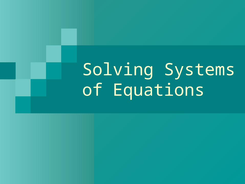
Rule of Thumb: •More equations than unknowns system is unlikely to have a solution. •Same number of equations as unknowns system is likely to have a unique solution. •Fewer equations than unknowns the system is likely to have infinitely many solutions.

Solving a System with Several Equations in Several Unknowns

We are interested in this last situation!

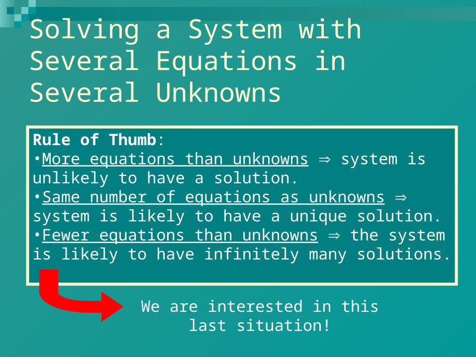
Systems of Equations

Linear system. Matrix methods.

1 2 3 1 2

1 3 1 2

1 2 3 1 2

2 2 2 11 0

4 2 5 0

5 0

y y y x x

y y x x

y y y x x

Note: We expect to have as many “free variables” as the difference between the number of unknowns and the number of equations.

Systems of Equations

43)cos(4

1)sin(3

tty

txy

Linear system. Matrix methods.

Non-linear system. Can be solved analytically

More difficult!

1 2 3 1 2

1 3 1 2

1 2 3 1 2

2 2 2 11 0

4 2 5 0

5 0

y y y x x

y y x x

y y y x x

cos( ) 3 sin( ) 4 0x y x y

Linear Systems of Equations

1 2 3 1 2

1 3 1 2

1 2 3 1 2

2 2 2 11 0

4 2 5 0

5 0

y y y x x

y y x x

y y y x x

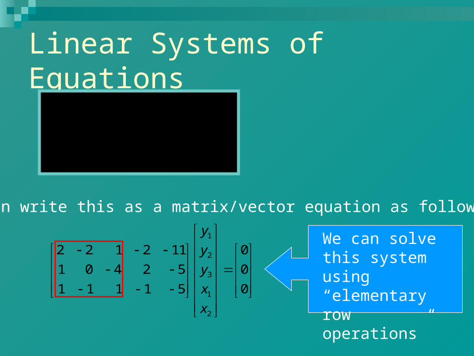
We can write this as a matrix/vector equation as follows:

1

2

3

1

2

2 2 1 2 11 0

1 0 4 2 5 0

1 1 1 1 5 0

y

y

y

x

x

We can solve this system using “elementary row operations”

Solving the System

1

2

3

1

2

1 0 0 2 1 0

0 1 0 3 5 0

0 0 1 0 1 0

y

y

y

x

x

1 0 0 2 1

0 1 0 3 5

0 0 1 0 1

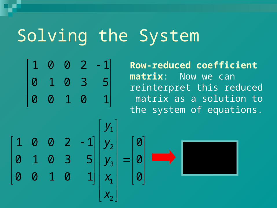
Row-reduced coefficient matrix: Now we can reinterpret this reduced matrix as a solution to the system of equations.

1 1 2

2 1 2

3 2

2

3 5

y x x

y x x

y x

The Solution Function

1 2 3 1 2

1 3 1 2

1 2 3 1 2

2 2 2 11 0

4 2 5 0

5 0

y y y x x

y y x x

y y y x x

1 1 2

2 1 2

3 2

2

3 5

y x x

y x x

y x

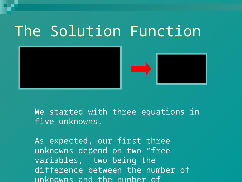
We started with three equations in five unknowns.

As expected, our first three unknowns depend on two “free variables,” two being the difference between the number of unknowns and the number of equations.

Where are we? Solving a system of m equations in n unknowns

is equivalent to finding the “zeros” of a vector valued function from

m→n. When m > n, such a system will “typically”

have infinitely many solutions. In “nice” cases, the solution will be a function from

m-n→n.

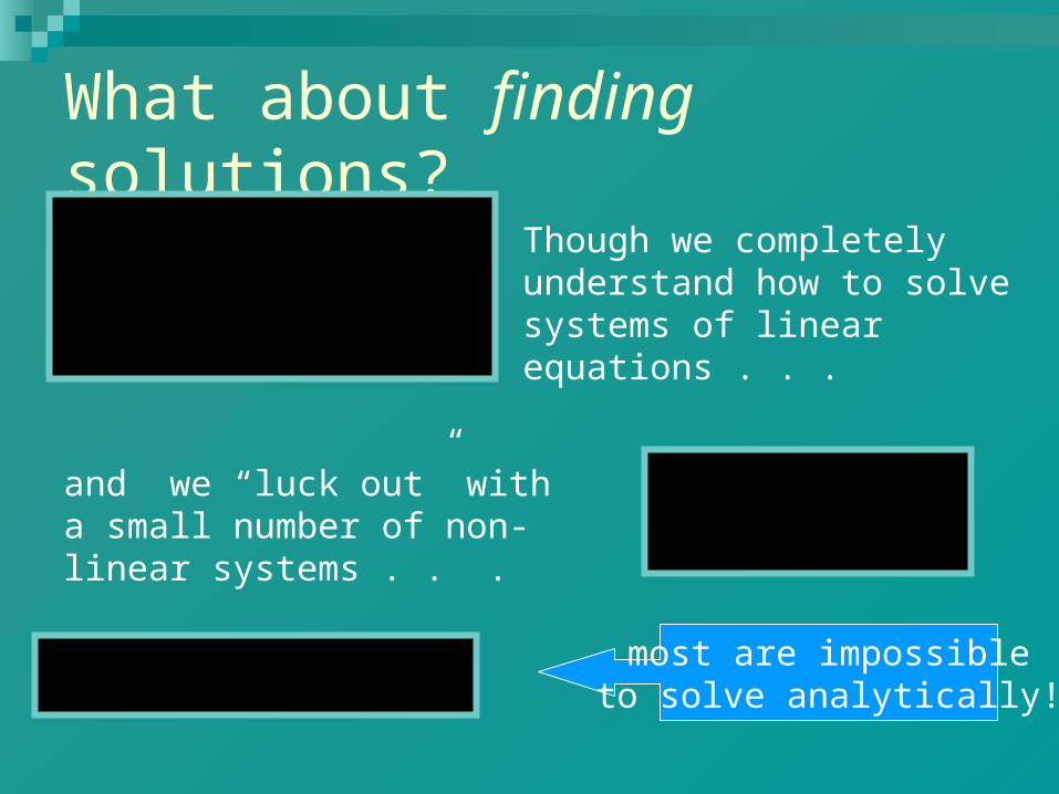
What about finding solutions?

43)cos(4

1)sin(3

tty

txy

most are impossibleto solve analytically!

1 2 3 1 2

1 3 1 2

1 2 3 1 2

2 2 2 11 0

4 2 5 0

5 0

y y y x x

y y x x

y y y x x

Though we completely understand how to solve systems of linear equations . . .

and we “luck out” with a small number of non-linear systems . . .

cos( ) 3 sin( ) 4 0x y x y

The Implicit Function Theorem. . .

Now we Introduce a useful theoretical framework

. . . gives us conditions under which a system of m equations in n unknowns will have a solution.

. . . and it tells us that (under reasonable hypotheses) the solution function will be well behaved.

1 2 3 1 2

1 3 1 2

1 2 3 1 2

2 2 2 11

4 2 5

5

y y y x x

y y x x

y y y x x

F 0

1 2

1 2 1 2

2

2

( , ) 3 5

x x

x x x x

x

g

1 2 3 1 2

1 3 1 2

1 2 3 1 2

2 2 2 11 0

4 2 5 0

5 0

y y y x x

y y x x

y y y x x

1 1 2 3 1 2

2 1 3 1 2

3 1 2 3 1 2

2 2 2 11 0

4 2 5 0

5 0

f y y y x x

f y y x x

f y y y x x

1 1 2

2 1 2

3 2

2

3 5

y x x

y x x

y x

F: 5 → 3

g : 2 → 3

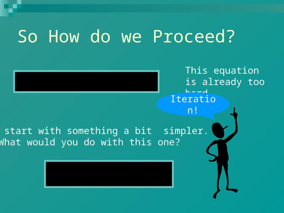
So How do we Proceed?

cos( ) 3 sin( ) 4 0x y x y This equation is already too hard….

We’ll start with something a bit simpler.What would you do with this one?

3 214 25 150 0

75x x x

So How do we Proceed?

cos( ) 3 sin( ) 4 0x y x y This equation is already too hard….

We’ll start with something a bit simpler.What would you do with this one?

3 214 25 150 0

75x x x

So How do we Proceed?

cos( ) 3 sin( ) 4 0x y x y This equation is already too hard….

We’ll start with something a bit simpler.What would you do with this one?

3 214 25 150 0

75x x x

Iteration!

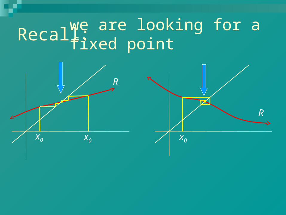
Recall:

x0 x0x0

R

R

we are looking for a fixed point

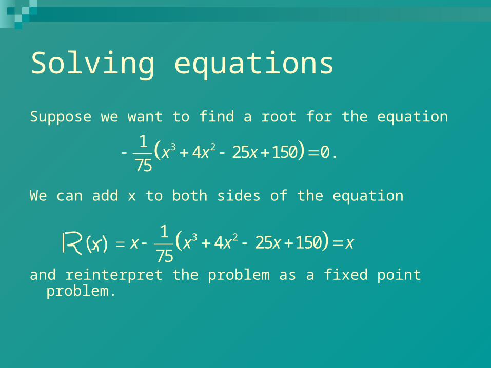
Solving equations

Suppose we want to find a root for the equation

We can add x to both sides of the equation

and reinterpret the problem as a fixed point problem.

3 214 25 150 0.

75x x x

3 214 25 150

75x x x x x

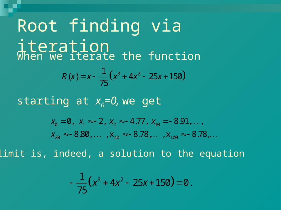
Root finding via iterationWhen we iterate the function

starting at x0=0, we get

3 21( ) 4 25 150

75R x x x x x

0 1 2 10

20 40 100

0, 2, 4.77, 8.91, ,

8.80, , x 8.78, , x 8.78,

x x x x

x

3 214 25 150 0.

75x x x

The limit is, indeed, a solution to the equation

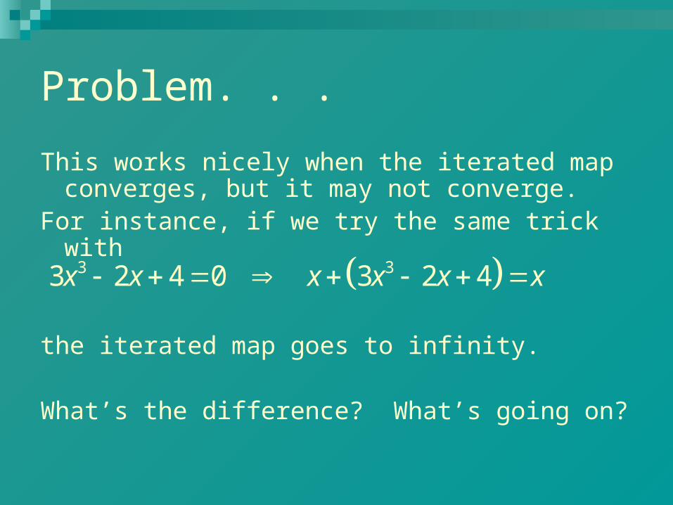
Problem. . .

This works nicely when the iterated map converges, but it may not converge.

For instance, if we try the same trick with

the iterated map goes to infinity.

What’s the difference? What’s going on?

3 33 2 4 0 3 2 4x x x x x x

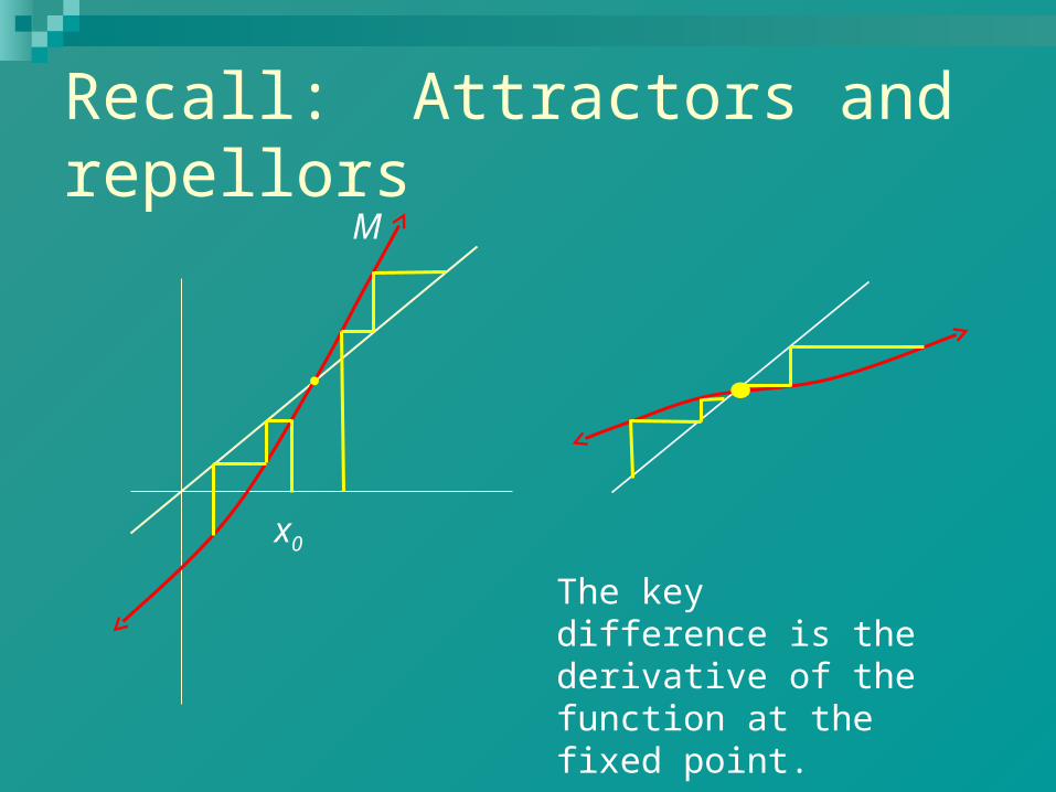
Recall: Attractors and repellors

x0

The key difference is the derivative of the function at the fixed point.

M

The Derivative at the Fixed Point

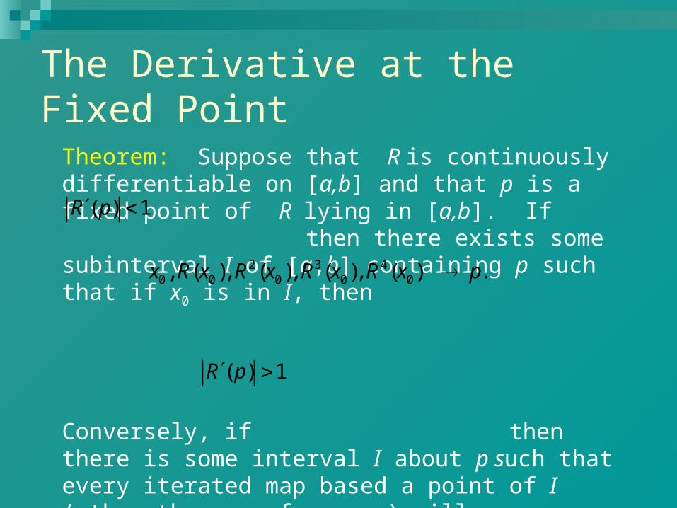
Theorem: Suppose that R is continuously differentiable on [a,b] and that p is a fixed point of R lying in [a,b]. If then there exists some subinterval I of [a,b] containing p such that if x0 is in I, then

Conversely, if then there is some interval I about p such that every iterated map based a point of I (other than p, of course) will eventually leave I and will thus not converge to p.

2 3 40 0 0 0 0, ( ), ( ), ( ), ( ) .x R x R x R x R x p

( ) 1R p

( ) 1R p

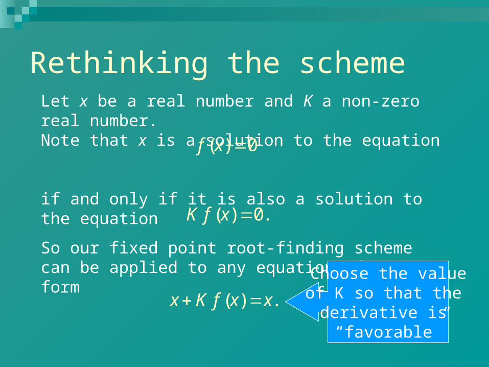
Let x be a real number and K a non-zero real number. Note that x is a solution to the equation

if and only if it is also a solution to the equation

Rethinking the scheme

( ) 0f x

( ) 0.K f x

So our fixed point root-finding scheme can be applied to any equation of the form

( ) .x K f x x Choose the valueof K so that the

derivative is “favorable”

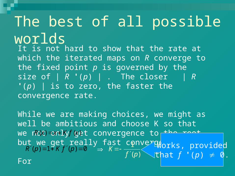
The best of all possible worldsIt is not hard to show that the rate at which the iterated maps on R converge to the fixed point p is governed by the size of | R '(p) | . The closer | R '(p) | is to zero, the faster the convergence rate.

While we are making choices, we might as well be ambitious and choose K so that we not only get convergence to the root, but we get really fast convergence!

For we want( ) ( )R x x K f x

( ) 1 ( ) 0R p K f p 1

( )K

f p

Works, providedthat f '(p) 0.

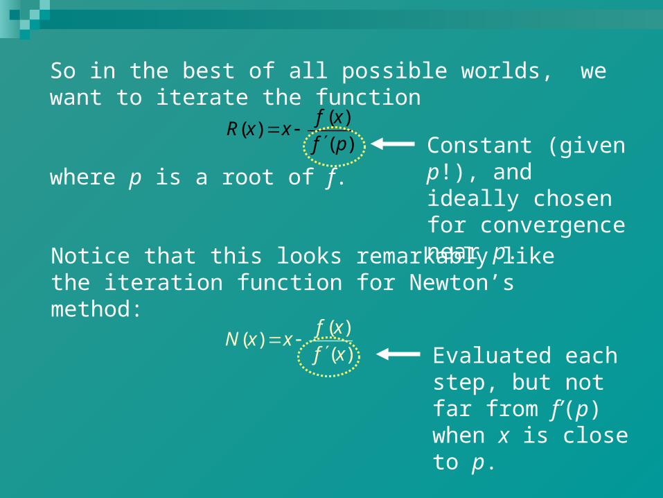
So in the best of all possible worlds, we want to iterate the function

where p is a root of f.

( )( )

( )

f xR x x

f p

Notice that this looks remarkably like the iteration function for Newton’s method:

( )( )

( )

f xN x x

f x

Constant (given p!), and ideally chosen for convergence near p.

Evaluated each step, but not far from f’(p) when x is close to p.

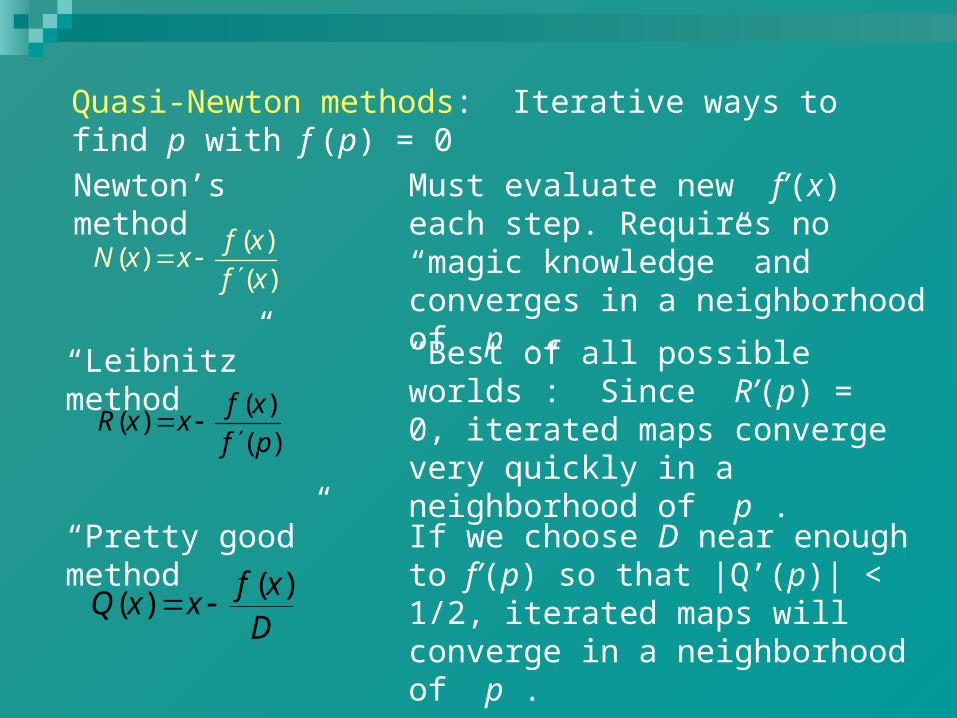
Quasi-Newton methods: Iterative ways to find p with f (p) = 0

Must evaluate new f’(x) each step. Requires no “magic knowledge” and converges in a neighborhood of p .

( )( )

( )

f xN x x

f x

Newton’s method

“Pretty good” method

Dxf

xxQ)(

)(

( )( )

( )

f xR x x

f p

“Leibnitz” method

If we choose D near enough to f’(p) so that |Q’(p)| < 1/2, iterated maps will converge in a neighborhood of p .

“Best of all possible worlds”: Since R’(p) = 0, iterated maps converge very quickly in a neighborhood of p .

One Equation in Two Unknowns

cos( ) 3 sin( ) 4 0?x y x y

Can we use this set of ideas to tackle

Yes!

First we recall that the solutions to this equation are the zeros of the 2-variable function

( , ) cos( ) 3 sin( ) 4f x y x y x y

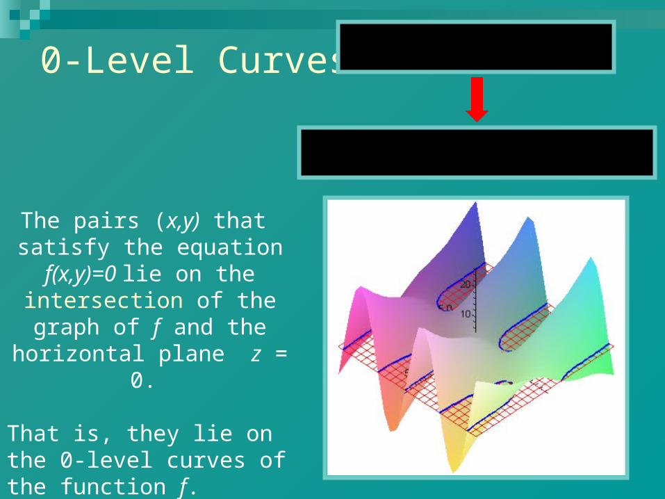
0-Level Curves

( , ) cos( ) 3 sin( ) 4 0f x y x y x y

cos( ) 3 sin( ) 4 0x y x y

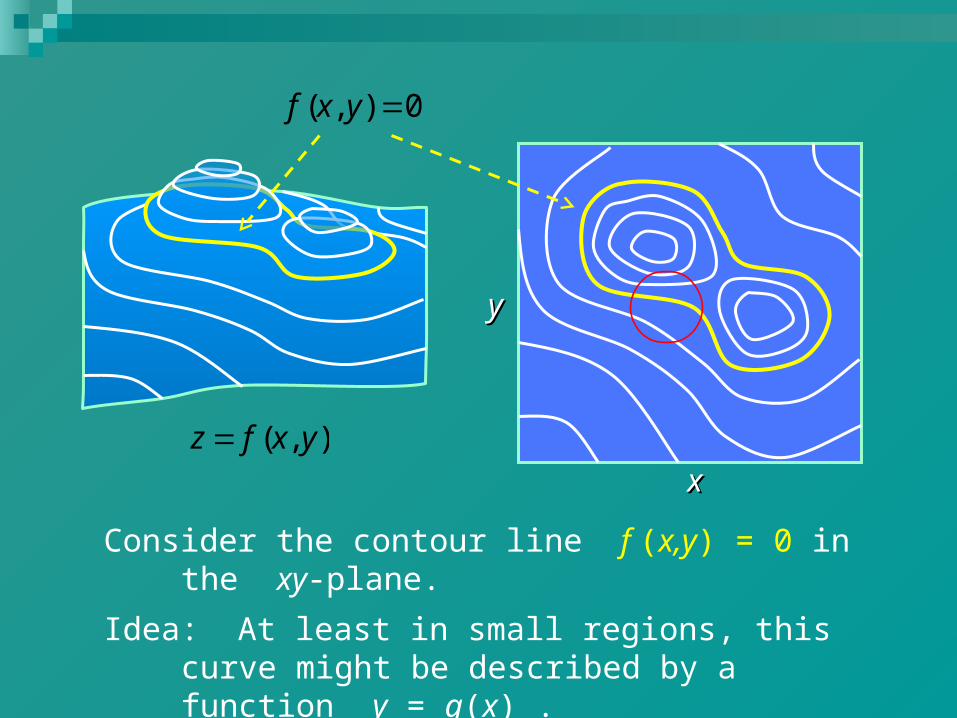
The pairs (x,y) that satisfy the equation f(x,y)=0 lie on the intersection of the graph of f

and the horizontal plane z = 0.

That is, they lie on the 0-level curves of the function f.

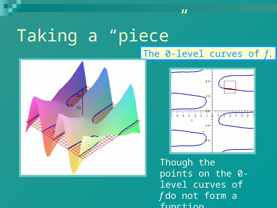
Taking a “piece”The 0-level curves of f.

Though the points on the 0-level curves of f do not form a function, portions of them do.

),( yxfz

0),( yxf

xx

yy

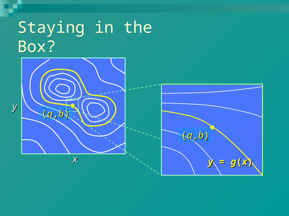
Consider the contour line f (x,y) = 0 in the xy-plane.

Idea: At least in small regions, this curve might be described by a function y = g(x) .

Our goal: find such a function!

xx

yy

0),(

bayf

D

((aa,,bb))

((aa,,bb))

yy = = gg((xx))

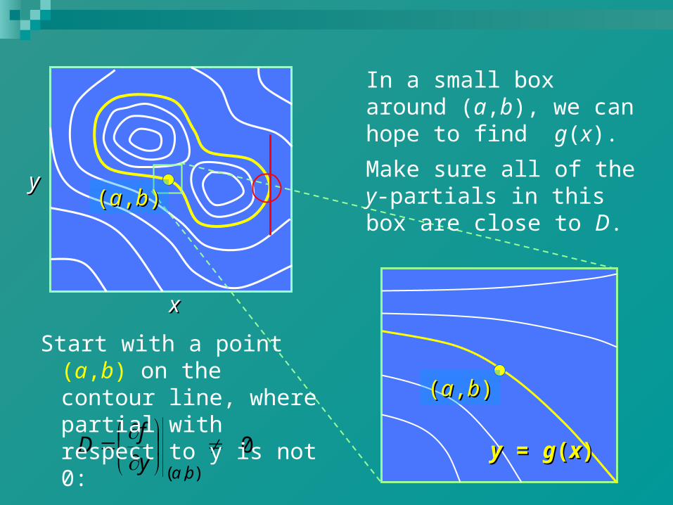
Start with a point (a,b) on the contour line, where partial with respect to y is not 0:

In a small box around (a,b), we can hope to find g(x).

Make sure all of the y-partials in this box are close to D.

D

yxfyyx

,((aa,,bb))

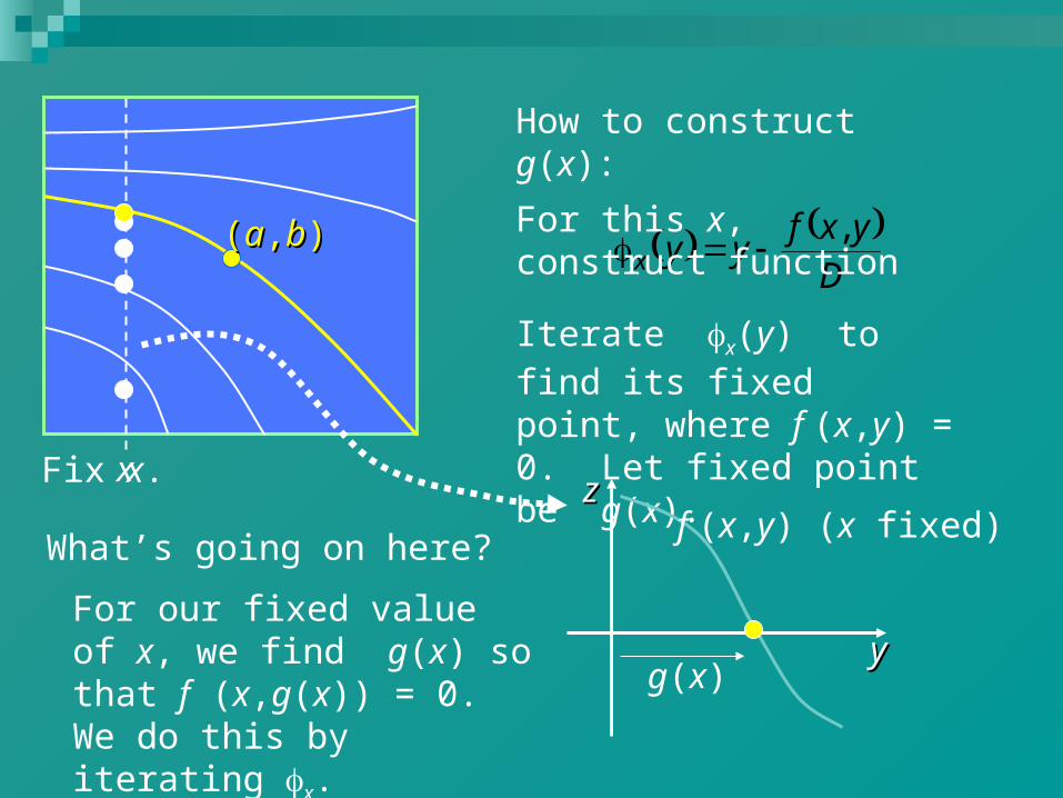
How to construct g(x):

For this x, construct function

Iterate x(y) to find its fixed point, where f (x,y) = 0. Let fixed point be g(x).

x

yy

zzf (x,y) (x fixed)

What’s going on here?

For our fixed value of x, we find g(x) so that f (x,g(x)) = 0. We do this by iterating x.

g(x)

Fix x.

D

yxfyyx

,((aa,,bb))

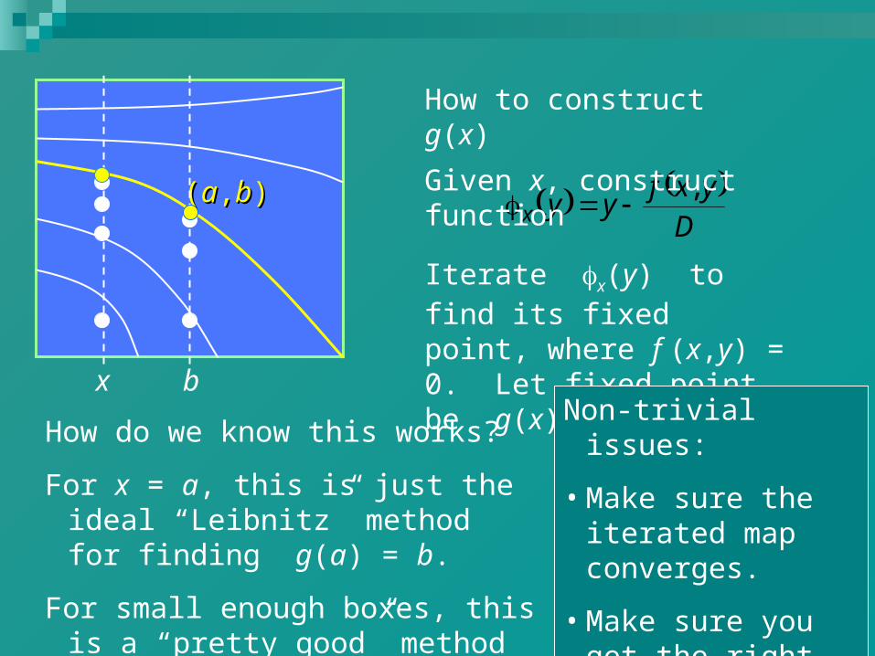
How to construct g(x)

Given x, construct function

Iterate x(y) to find its fixed point, where f (x,y) = 0. Let fixed point be g(x).

x

How do we know this works?

For x = a, this is just the ideal “Leibnitz” method for finding g(a) = b.

For small enough boxes, this is a “pretty good” method elsewhere.

Non-trivial issues:

• Make sure the iterated map converges.

• Make sure you get the right fixed point. (Don’t leave the box!)

b

xx

yy((aa,,bb))

((aa,,bb))

yy = = gg((xx))

Staying in the Box?

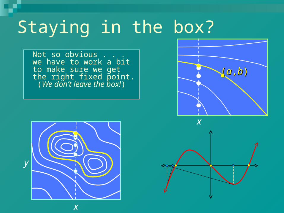
Staying in the box? Not so obvious . . . we

have to work a bit to make sure we get the right fixed point. (We don’t leave the box!)

((aa,,bb))

x

y

x

Looking ahead

We are interested in solving systems of equations.

The Implicit Function Theorem will tell us when there are solutions to a system and will describe the nature of those solutions.

We will prove the implicit function theorem by employing quasi-Newton’s methods as a theoretical tool.