HAL Id: hal-00715301https://hal.archives-ouvertes.fr/hal-00715301

Submitted on 6 Jul 2012

HAL is a multi-disciplinary open accessarchive for the deposit and dissemination of sci-entific research documents, whether they are pub-lished or not. The documents may come fromteaching and research institutions in France orabroad, or from public or private research centers.

L’archive ouverte pluridisciplinaire HAL, estdestinée au dépôt et à la diffusion de documentsscientifiques de niveau recherche, publiés ou non,émanant des établissements d’enseignement et derecherche français ou étrangers, des laboratoirespublics ou privés.

Solving Shallow Water flows in 2D with FreeFem++ onstructured mesh

Georges Sadaka

To cite this version:Georges Sadaka. Solving Shallow Water flows in 2D with FreeFem++ on structured mesh. 2012.<hal-00715301>

Solving Shallow Water flows in 2D with

FreeFem++ on structured mesh

Georges Sadaka

LAMFA CNRS UMR 7352

Universite de Picardie Jules Verne

33, rue Saint-Leu, 80039 Amiens, France

http://lamfa.u-picardie.fr/sadaka/

k georges.sadaka@u-picardie.fr

Abstract - FreeFem++ is an open source platform to solve partial differential equationsnumerically, based on finite element methods. What we will present in this work is inspired fromthe finite volume method for hyperbolic problem in order to solve it with finite element method inFreeFem++. In particular we will see how it can be possible, with an approach of finite elementand finite volume method, to solve the Shallow Water equations (Saint - Venant system) in 2Dwith topographic source term. More precisely, we will define the quantity types of finite volumesuch as up-wind scheme, HLL flux, well balanced scheme with hydrostatic reconstruction that areused in the numerical resolution of the variational problem.

To this end we will consider a particular rectangular structured isotropic domain using P1 finiteelement space. We note that in other situations, for example with unstructured anisotropic meshor with other type of finite element space, an approach of Discontinuous Galerkin method could beused as in [11]. We note also that, there is a FreeVol project in order to introduce Finite Volumetechnic in FreeFem++ for hyperbolic PDEs by Frederic Hecht et al. which is an ongoing work.

Keywords: Shallow Water equations, finite volume method, finite element method, well-balancedscheme, hydrostatic reconstruction, FreeFem++.

1 Introduction

The Shallow Water equations introduced in [12] is very commonly used for the numericalsimulation of various geophysical shallow-water flows [2], such as rivers [4], lakes or coastal areas[6], rainfall runoff on agricultural fields [9], or even atmosphere or avalanches [1, 8] when completedwith appropriate source terms.

The numerical study of damped hydrodynamic surface wave propagation is a very challengingproblem through the phenomena that represent (giant waves, Tsunamis, ...). The shallow waterequations are routinely used to predict a tsunami wave Run-up and, subsequently, constituteinundation maps for tsunami hazard areas.

Our motivation in this paper comes from the oscillation that we see during our simulations, usingthe Boussinesq system in 2D, with the propagation of Tsunamis near the coast where we are not inthe big deep water wave regime (cf. [17]).

To solve this problem, we must consider another regime for small deep water wave for example theShallow Water equations in order also to see the inundation of the Tsunamis. Many works haveconsider this problem from a finite volume point of view to construct approximate solutions for the

1

hyperbolic conservation laws where they build a well balanced scheme which preserve the positivityof the solution during the Run-up (cf. [3, 7, 13, 16]).

The two-dimensional Saint-Venant system for Shallow Water writes as follows :

∂tU + ∂xF (U) + ∂yG(U) = S(U), (1)

where

U =

hhuhv

, F (U) =

hu

hu2 +g

2h2

huv

, G(U) =

hvhuv

hv2 +g

2h2

and S(U) =

0−gh∂xzb−gh∂yzb

.

(2)Here u and v are the scalar components in the horizontal x, y directions of the depth-averagedvelocity, h is the local water depth and g > 0 denotes the gravity constant. U is the vector for theconservative variables, F (U) and G(U) stand for the flux functions respectively along the x and y

directions and S(U) represents the bed slope source term with the bed slope ∇zb =

(∂xzb∂yzb

).

This model is very robust, being hyperbolic and admitting an entropy inequality (related to thephysical energy E, see [18] for more details)

∂tE(U, zb) + ∂x

[u ·(E(U, zb) +

gh2

2

)]+ ∂y

[v ·(E(U, zb) +

gh2

2

)]≤ 0 (3)

whereE(U) = (hu2 + hv2)/2 +

g

2h2 and E(U, zb) = E(U) + hgzb. (4)

Another nice property is that it preserves the steady state of a lake at rest

h+ zb = Cst, u = 0, v = 0. (5)

When solving numerically (1), it is very important to be able to preserve these steady states at thediscrete level and to accurately compute the evolution of small deviations from them, because themajority of real-life applications resides in this flow regime. It is a difficult problem identified forthe first time in [5] and the scheme which preserves this type of equilibrium are called wellbalanced since [14].

The paper is organized as follows. In Section 2 we remind the construction of the well-balancedscheme with hydrostatic reconstruction. In Section 3 the HLL approximate Riemann solver ispresented for the wet/dry transition problem. In Section 4, we present the corresponding CFLcondition in order to have the stability of the up-wind scheme. We present in Section 5 the detailsof the finite volume approach in FreeFem++ by giving the corresponding code for each step.Finally, in Section 6 we present the numerical simulations starting by testing the correctness andprecision of the numerical scheme using an analytical solution, then by showing the simulation of asolitary wave crossing an empty pond.

2 Well-balanced scheme with hydrostatic reconstruction

The system (1) can be written as :

∂tU + A(U)∂xU + B(U)∂yU = S(U), (6)

where

A(U) =

0 1 0−u2 + gh 2u 0−uv v u

and B(U) =

0 0 1−uv v u

−v2 + gh 0 2v

,

2

thendet(A(U)− λI) = (u− λ) · (λ− u−

√gh) · (λ− u+

√gh)

anddet(B(U)− λI) = (v − λ) · (λ− v −

√gh) · (λ− v +

√gh).

Thus, the eigenvalues of the linearized convection matrices A(U) and B(U) are, respectively :

λ1 = u, λ2 = u−√gh, λ3 = u+

√gh and λ∗1 = v, λ∗2 = v −

√gh, λ∗3 = v +

√gh (7)

We remark that for h > 0, all the eigenvalues are distinct and the system is strictly hyperbolic.Finite volume schemes for hyperbolic systems consist in using an up-winding of the fluxes. Thetwo-dimensional semi-discrete finite volume formulation of system (1) with hydrostaticreconstruction, is given by :

Un+1i,j −Un

i,j +∆t

∆x

(Fn

i+1/2,j − Fni−1/2,j

)+

∆t

∆y

(Gn

i,j+1/2 −Gni,j−1/2

)= ∆t · Sn

i,j (8)

where

Fni+1/2,j = F

(Ui+1/2,j,L,Ui+1/2,j,R

), Fn

i−1/2,j = F(Ui−1/2,j,L,Ui−1/2,j,R

),

Gni,j+1/2 = G

(Ui,j+1/2,D,Ui,j+1/2,U

), Gn

i,j−1/2 = G(Ui,j−1/2,D,Ui,j−1/2,U

),

(9)

and

Sni,j =

01

∆x

(g2h

2i+1/2,j,L − g

2h2i−1/2,j,R

)

1∆y

(g2h

2i,j+1/2,D − g

2h2i,j−1/2,U

)

. (10)

Here F and G are the numerical flux to be define in the sequel and the evaluation of the cellinterface of the conservative variables are defined as :

Ui−1/2,j,L =

hi−1/2,j,L

hi−1/2,j,L · ui−1,j

hi−1/2,j,L · vi−1,j

,Ui−1/2,j,R =

hi−1/2,j,R

hi−1/2,j,R · ui,jhi−1/2,j,R · vi,j

,

Ui+1/2,j,L =

hi+1/2,j,L

hi+1/2,j,L · ui,jhi+1/2,j,L · vi,j

,Ui+1/2,j,R =

hi+1/2,j,R

hi+1/2,j,R · ui+1,j

hi+1/2,j,R · vi+1,j

,

Ui,j−1/2,D =

hi,j−1/2,D

hi,j−1/2,D · ui,j−1

hi,j−1/2,D · vi,j−1

,Ui,j−1/2,U =

hi,j−1/2,U

hi,j−1/2,U · ui,jhi,j−1/2,U · vi,j

,

and

Ui,j+1/2,D =

hi,j+1/2,D

hi,j+1/2,D · ui,jhi,j+1/2,D · vi,j

,Ui,j+1/2,U =

hi,j+1/2,U

hi,j+1/2,U · ui,j+1

hi,j+1/2,U · vi,j+1

.

We use the notation U for Up, L for Left, R for Right and D for Down (cf. Figure 1).This ansatz is motivated by a balancing requirement, as follows. For nearly hydrostatic flows onehas u √gh and v √gh. In the associated asymptotic limit the leading order water height hadjusts so as to satisfy the balance of momentum flux and momentum source terms, i.e.

∂x

(gh2

2

)= −hg∂xzb and ∂y

(gh2

2

)= −hg∂yzb. (11)

Integrating over the (i, j)-th grid cell, we obtain an approximation to the net source term as

−∫ xi+1/2,j

xi−1/2,j

hg∂xzbdx =g

2h2i+1/2,j,L −

g

2h2i−1/2,j,R

3

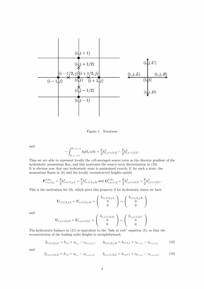
Figure 1: Notations

and

−∫ yi,j+1/2

yi,j−1/2

hg∂yzbdy =g

2h2i,j+1/2,D −

g

2h2i,j−1/2,U .

Thus we are able to represent locally the cell-averaged source term as the discrete gradient of thehydrostatic momentum flux, and this motivates the source term discretization in (10).It is obvious now that any hydrostatic state is maintained exactly if, for such a state, themomentum fluxes in (8) and the locally reconstructed heights satisfy

Fn,hui+1/2,j =

g

2h2i+1/2,j,L =

g

2h2i+1/2,j,R and Gn,hv

i,j+1/2 =g

2h2i,j+1/2,D =

g

2h2i,j+1/2,U .

This is the motivation for (9), which gives this property if for hydrostatic states we have

Ui+1/2,j,L = Ui+1/2,j,R =

hi+1/2,j,L

00

=

hi+1/2,j,R

00

and

Ui,j+1/2,D = Ui,j+1/2,U =

hi,j+1/2,D

00

=

hi,j+1/2,U

00

.

The hydrostatic balance in (11) is equivalent to the “lake at rest” equation (5), so that thereconstruction of the leading order heights is straightforward,

hi+1/2,j,L = hi,j + zbi,j − zbi+1/2,j, hi+1/2,j,R = hi+1,j + zbi+1,j − zbi+1/2,j

(12)

andhi,j+1/2,D = hi,j + zbi,j − zbi,j+1/2

, hi,j+1/2,U = hi,j+1 + zbi,j+1 − zbi,j+1/2. (13)

4

An important challenge is to design a scheme that robustly captures dry regions where h ≡ 0. Inorder to ensure non negativity of the water height even when cells begin to “dry out”, we need firstto perform a truncation of the leading order heights in (12,13),

hi+1/2,j,L/R = max(

0, hi+1/2,j,L/R

)and hi,j+1/2,D/U = max

(0, hi,j+1/2,D/U

). (14)

Next, the evaluation of the cell interface height zbi+1/2,jand zbi,j+1/2

has to be done in a quitesubtle way. Our construction, combined with a centered value of zbi+1/2,j

and zbi,j+1/2, is not stable.

We rather take an upwind evaluation of the form

zbi+1/2,j= max

(zbi,j , zbi+1,j

)and zbi,j+1/2

= max(zbi,j , zbi,j+1

). (15)

With these choices, we ensure that 0 ≤ hi+1/2,j,L ≤ hi,j and 0 ≤ hi+1/2,j,R ≤ hi+1,j also that0 ≤ hi,j+1/2,D ≤ hi,j and 0 ≤ hi,j+1/2,U ≤ hi,j+1 , and we prove below that this property ensuresthe non negativity requirement.

3 HLL approximate Riemann solver

We implement here the HLL (Harten, Lax and van Leer) approximate Riemann solver proposed in[15]. When working on dry bed problems the HLL approach highlights a better behavior, avoidingunidimensionalisation effects on the flow field. Such a reason leads to the choice of the HLLRiemann solver for the development of the presented code.

The application of this approach to the two-dimensional scheme gives the following expression forthe numerical flux:

F(a,b) =

F (a) if 0 < sL,F (b) if sR < 0,sR · F (a)− sL · F (b) + sL · sR · (b− a)

sR − sLif sL ≤ 0 ≤ sR,

(16)

where

sL = infc=a,b

(inf

i∈1,2,3(λi(c))

)and sR = sup

c=a,b

(sup

i∈1,2,3(λi(c))

), (17)

and

G(a,b) =

G(a) if 0 < sD,G(b) if sU < 0,sU ·G(a)− sD ·G(b) + sD · sU · (b− a)

sU − sDif sD ≤ 0 ≤ sU ,

(18)

where

sD = infc=a,b

(inf

i∈1,2,3(λ∗i (c))

)and sU = sup

c=a,b

(sup

i∈1,2,3(λ∗i (c))

). (19)

4 Numerical stability

Explicit schemes require a careful selection of the time step to fulfill stability requirements.Classically, the time step needs to be restricted in such a way that no interaction is possiblebetween waves from different cells during each time step. Courant, Friedrichs and Lewy defined astability criterion for fully explicit schemes given by CFL < 1 where CFL is known as the Courantnumber. Various definitions of this number have been proposed, leading to different time steprestrictions. As in [7] , we choose here to define the time step as follows:

∆t ≤ CFLmin(∆x,∆y)

max(|uL|+ cL; |uR|+ cR; |vD|+ cD; |vU |+ cU

) ; (20)

5

where

uL = ui+1/2,j,L;hL = hi+1/2,j,L; cL =√g · hL;uR = ui+1/2,j,R;hR = hi+1/2,j,R; cR =

√g · hR

and

vD = vi,j+1/2,D;hD = hi,j+1/2,D; cD =√g · hD; vU = vi,j+1/2,U ;hU = hi,j+1/2,U ; cU =

√g · hU .

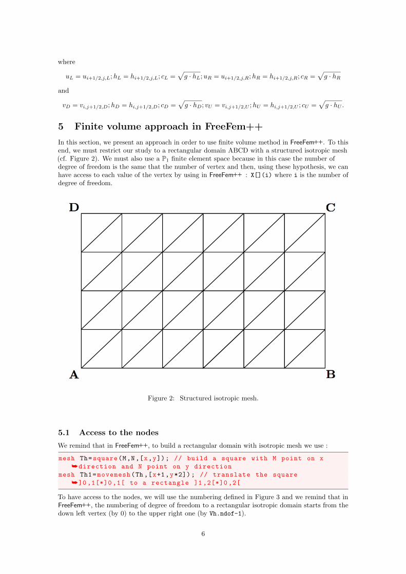
5 Finite volume approach in FreeFem++

In this section, we present an approach in order to use finite volume method in FreeFem++. To thisend, we must restrict our study to a rectangular domain ABCD with a structured isotropic mesh(cf. Figure 2). We must also use a P1 finite element space because in this case the number ofdegree of freedom is the same that the number of vertex and then, using these hypothesis, we canhave access to each value of the vertex by using in FreeFem++ : X[](i) where i is the number ofdegree of freedom.

Figure 2: Structured isotropic mesh.

5.1 Access to the nodes

We remind that in FreeFem++, to build a rectangular domain with isotropic mesh we use :

mesh Th=square(M,N,[x,y]); // build a square with M point on x

ådirection and N point on y direction

mesh Th1=movemesh(Th ,[x+1,y*2]); // translate the square

å]0 ,1[*]0 ,1[ to a rectangle ]1 ,2[*]0 ,2[

To have access to the nodes, we will use the numbering defined in Figure 3 and we remind that inFreeFem++, the numbering of degree of freedom to a rectangular isotropic domain starts from thedown left vertex (by 0) to the upper right one (by Vh.ndof-1).

6

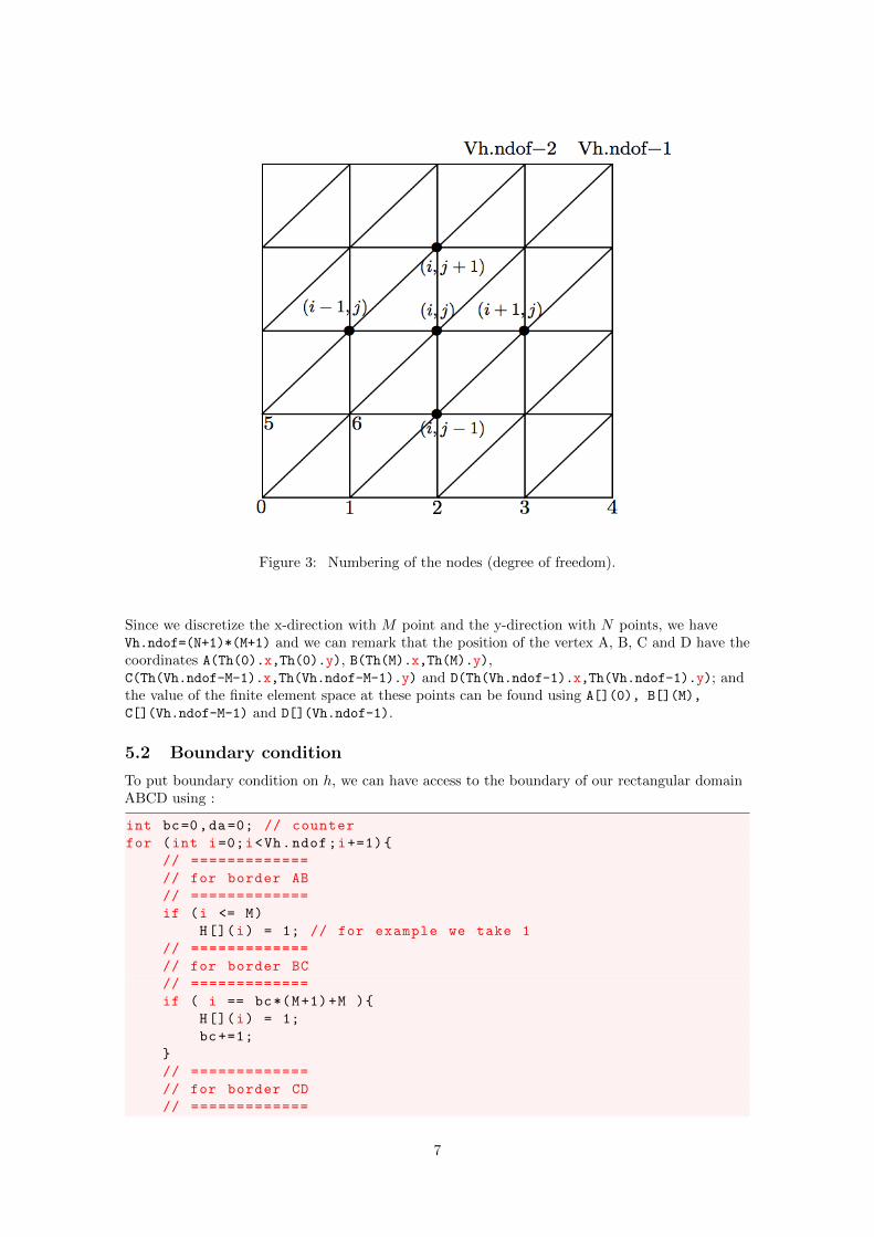
Figure 3: Numbering of the nodes (degree of freedom).

Since we discretize the x-direction with M point and the y-direction with N points, we haveVh.ndof=(N+1)*(M+1) and we can remark that the position of the vertex A, B, C and D have thecoordinates A(Th(0).x,Th(0).y), B(Th(M).x,Th(M).y),C(Th(Vh.ndof-M-1).x,Th(Vh.ndof-M-1).y) and D(Th(Vh.ndof-1).x,Th(Vh.ndof-1).y); andthe value of the finite element space at these points can be found using A[](0), B[](M),

C[](Vh.ndof-M-1) and D[](Vh.ndof-1).

5.2 Boundary condition

To put boundary condition on h, we can have access to the boundary of our rectangular domainABCD using :

int bc=0,da=0; // counter

for (int i=0;i<Vh.ndof;i+=1)

// =============

// for border AB

// =============

if (i <= M)

H[](i) = 1; // for example we take 1

// =============

// for border BC

// =============

if ( i == bc*(M+1)+M )

H[](i) = 1;

bc+=1;

// =============

// for border CD

// =============

7

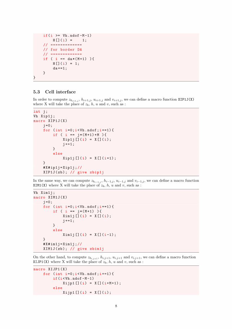
if(i >= Vh.ndof -M-1)

H[](i) = 1;

// =============

// for border DA

// =============

if ( i == da*(M+1) )

H[](i) = 1;

da+=1;

5.3 Cell interface

In order to compute zbi+1,j , hi+1,j , ui+1,j and vi+1,j , we can define a macro function XIP1J(X)

where X will take the place of zb, h, u and v, such as :

int j;

Vh Xip1j;

macro XIP1J(X)

j=0;

for (int i=0;i<Vh.ndof;i+=1)

if ( i == j*(M+1)+M )

Xip1j [](i) = X[](i);

j+=1;

else

Xip1j [](i) = X[](i+1);

#X#ip1j=Xip1j;//

XIP1J(zb); // give zbip1j

In the same way, we can compute zbi−1,j, hi−1,j , ui−1,j and vi−1,j , we can define a macro function

XIM1(X) where X will take the place of zb, h, u and v, such as :

Vh Xim1j;

macro XIM1J(X)

j=0;

for (int i=0;i<Vh.ndof;i+=1)

if ( i == j*(M+1) )

Xim1j [](i) = X[](i);

j+=1;

else

Xim1j [](i) = X[](i-1);

#X#im1j=Xim1j;//

XIM1J(zb); // give zbim1j

On the other hand, to compute zbi,j+1, hi,j+1, ui,j+1 and vi,j+1, we can define a macro function

XIJP1(X) where X will take the place of zb, h, u and v, such as :

macro XIJP1(X)

for (int i=0;i<Vh.ndof;i+=1)

if(i<Vh.ndof -M-1)

Xijp1 [](i) = X[](i+M+1);

else

Xijp1 [](i) = X[](i);

8

#X#ijp1=Xijp1;//

XIJP1(zb); // give zbijp1

macro XIJM1(X)

for (int i=0;i<Vh.ndof;i+=1)

if (i<=M)

Xijm1 [](i) = X[](i);

else if(i>M)

Xijm1 [](i) = X[](i-M-1);

#X#ijm1=Xijm1;//

XIJM1(zb); // give zbijm1

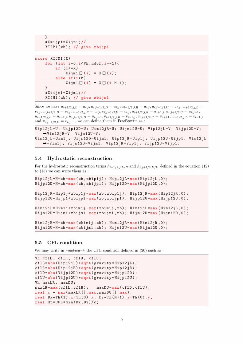
Since we have ui+1/2,j,L = ui,j , ui,j+1/2,D = ui,j , ui−1/2,j,R = ui,j , ui,j−1/2,U = ui,j , vi+1/2,j,L =vi,j , vi,j+1/2,D = vi,j , vi−1/2,j,R = vi,j , vi,j−1/2,U = vi,j , ui+1/2,j,R = ui+1,j , ui,j+1/2,U = ui,j+1,ui−1/2,j,L = ui−1,j , ui,j−1/2,D = ui,j−1, vi+1/2,j,R = vi+1,j , vi,j+1/2,U = vi,j+1, vi−1/2,j,L = vi−1,j

and vi,j−1/2,D = vi,j−1, we can define them in FreeFem++ as :

Uip12jL=U; Uijp12D=U; Uim12jR=U; Uijm12U=U; Vip12jL=V; Vijp12D=V;

åVim12jR=V; Vijm12U=V;

Uim12jL=Uim1j; Uijm12D=Uijm1; Uip12jR=Uip1j; Uijp12U=Uijp1; Vim12jL

å=Vim1j; Vijm12D=Vijm1; Vip12jR=Vip1j; Vijp12U=Vijp1;

5.4 Hydrostatic reconstruction

For the hydrostatic reconstruction terms hi+1/2,j,L/R and hi,j+1/2,D/U defined in the equation (12)to (15) we can write them as :

Hip12jL=H+zb -max(zb ,zbip1j); Hip12jL=max(Hip12jL ,0);

Hijp12D=H+zb -max(zb ,zbijp1); Hijp12D=max(Hijp12D ,0);

Hip12jR=Hip1j+zbip1j -max(zb ,zbip1j); Hip12jR=max(Hip12jR ,0);

Hijp12U=Hijp1+zbijp1 -max(zb ,zbijp1); Hijp12U=max(Hijp12U ,0);

Him12jL=Him1j+zbim1j -max(zbim1j ,zb); Him12jL=max(Him12jL ,0);

Hijm12D=Hijm1+zbijm1 -max(zbijm1 ,zb); Hijm12D=max(Hijm12D ,0);

Him12jR=H+zb -max(zbim1j ,zb); Him12jR=max(Him12jR ,0);

Hijm12U=H+zb -max(zbijm1 ,zb); Hijm12U=max(Hijm12U ,0);

5.5 CFL condition

We may write in FreeFem++ the CFL condition defined in (20) such as :

Vh cflL , cflR , cflD , cflU;

cflL=abs(Uip12jL)+sqrt(gravity*Hip12jL);

cflR=abs(Uip12jR)+sqrt(gravity*Hip12jR);

cflD=abs(Vijp12D)+sqrt(gravity*Hijp12D);

cflU=abs(Vijp12U)+sqrt(gravity*Hijp12U);

Vh maxLR , maxDU;

maxLR=max(cflL ,cflR); maxDU=max(cflD ,cflU);

real c = max(maxLR [].max ,maxDU []. max);

real Dx=Th(1).x-Th(0).x, Dy=Th(M+1).y-Th(0).y;

real dt=CFL*min(Dx ,Dy)/c;

9

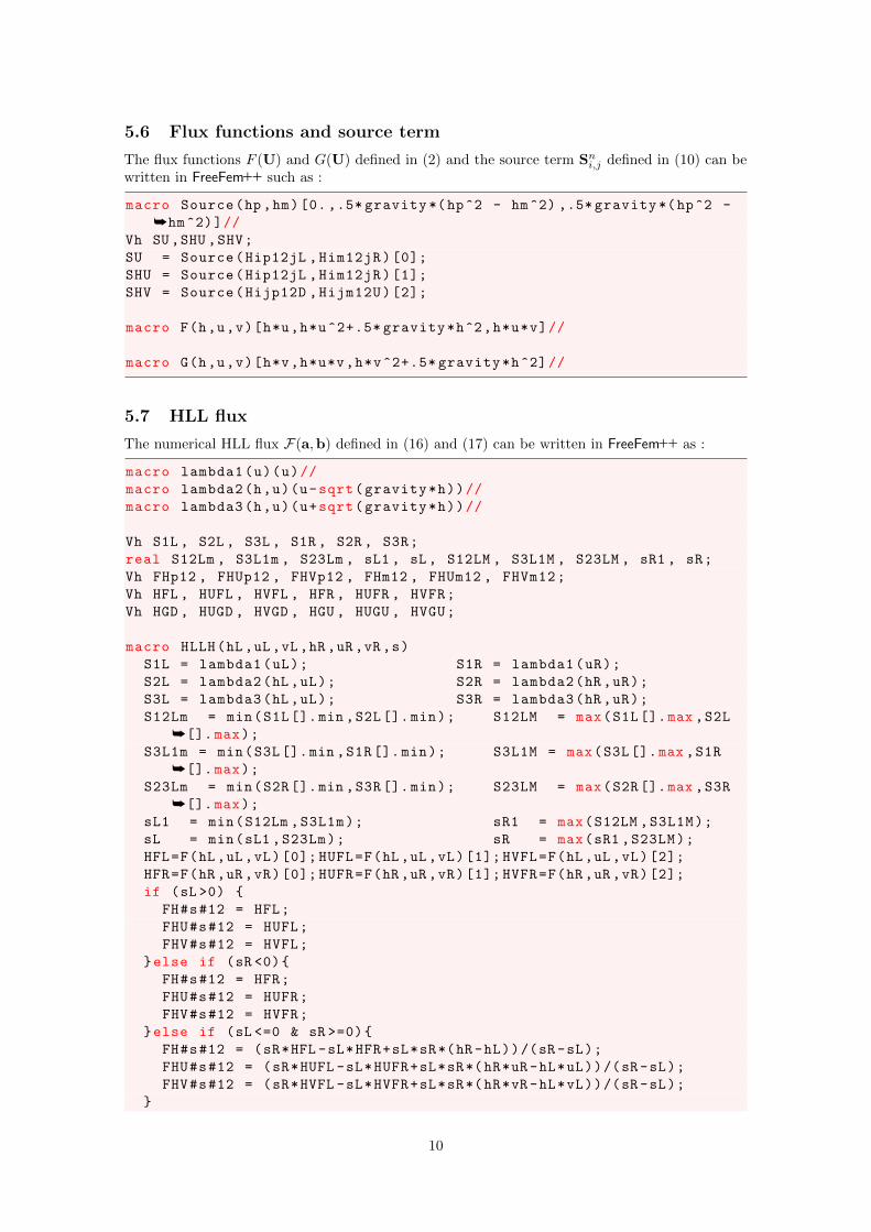
5.6 Flux functions and source term

The flux functions F (U) and G(U) defined in (2) and the source term Sni,j defined in (10) can be

written in FreeFem++ such as :

macro Source(hp,hm)[0. ,.5* gravity *(hp^2 - hm^2) ,.5* gravity *(hp^2 -

åhm^2)]//

Vh SU,SHU ,SHV;

SU = Source(Hip12jL ,Him12jR)[0];

SHU = Source(Hip12jL ,Him12jR)[1];

SHV = Source(Hijp12D ,Hijm12U)[2];

macro F(h,u,v)[h*u,h*u^2+.5* gravity*h^2,h*u*v]//

macro G(h,u,v)[h*v,h*u*v,h*v^2+.5* gravity*h^2]//

5.7 HLL flux

The numerical HLL flux F(a,b) defined in (16) and (17) can be written in FreeFem++ as :

macro lambda1(u)(u)//

macro lambda2(h,u)(u-sqrt(gravity*h))//

macro lambda3(h,u)(u+sqrt(gravity*h))//

Vh S1L , S2L , S3L , S1R , S2R , S3R;

real S12Lm , S3L1m , S23Lm , sL1 , sL , S12LM , S3L1M , S23LM , sR1 , sR;

Vh FHp12 , FHUp12 , FHVp12 , FHm12 , FHUm12 , FHVm12;

Vh HFL , HUFL , HVFL , HFR , HUFR , HVFR;

Vh HGD , HUGD , HVGD , HGU , HUGU , HVGU;

macro HLLH(hL,uL,vL,hR,uR,vR,s)

S1L = lambda1(uL); S1R = lambda1(uR);

S2L = lambda2(hL ,uL); S2R = lambda2(hR ,uR);

S3L = lambda3(hL ,uL); S3R = lambda3(hR ,uR);

S12Lm = min(S1L[].min ,S2L[].min); S12LM = max(S1L[].max ,S2L

å[].max);

S3L1m = min(S3L[].min ,S1R[].min); S3L1M = max(S3L[].max ,S1R

å[].max);

S23Lm = min(S2R[].min ,S3R[].min); S23LM = max(S2R[].max ,S3R

å[].max);

sL1 = min(S12Lm ,S3L1m); sR1 = max(S12LM ,S3L1M);

sL = min(sL1 ,S23Lm); sR = max(sR1 ,S23LM);

HFL=F(hL ,uL ,vL)[0]; HUFL=F(hL ,uL ,vL)[1]; HVFL=F(hL ,uL ,vL)[2];

HFR=F(hR ,uR ,vR)[0]; HUFR=F(hR ,uR ,vR)[1]; HVFR=F(hR ,uR ,vR)[2];

if (sL >0)

FH#s#12 = HFL;

FHU#s#12 = HUFL;

FHV#s#12 = HVFL;

else if (sR <0)

FH#s#12 = HFR;

FHU#s#12 = HUFR;

FHV#s#12 = HVFR;

else if (sL <=0 & sR >=0)

FH#s#12 = (sR*HFL -sL*HFR+sL*sR*(hR -hL))/(sR -sL);

FHU#s#12 = (sR*HUFL -sL*HUFR+sL*sR*(hR*uR -hL*uL))/(sR -sL);

FHV#s#12 = (sR*HVFL -sL*HVFR+sL*sR*(hR*vR -hL*vL))/(sR -sL);

10

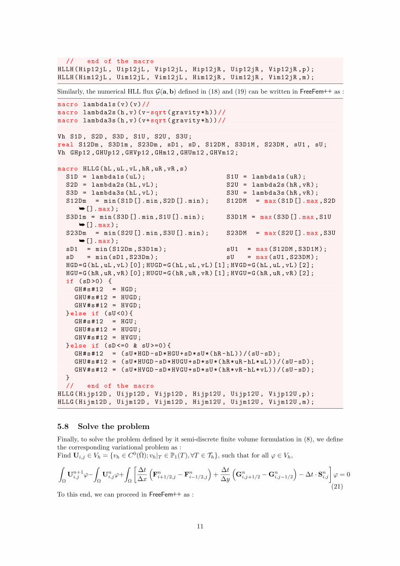
// end of the macro

HLLH(Hip12jL , Uip12jL , Vip12jL , Hip12jR , Uip12jR , Vip12jR ,p);

HLLH(Him12jL , Uim12jL , Vim12jL , Him12jR , Uim12jR , Vim12jR ,m);

Similarly, the numerical HLL flux G(a,b) defined in (18) and (19) can be written in FreeFem++ as :

macro lambda1s(v)(v)//

macro lambda2s(h,v)(v-sqrt(gravity*h))//

macro lambda3s(h,v)(v+sqrt(gravity*h))//

Vh S1D , S2D , S3D , S1U , S2U , S3U;

real S12Dm , S3D1m , S23Dm , sD1 , sD , S12DM , S3D1M , S23DM , sU1 , sU;

Vh GHp12 ,GHUp12 ,GHVp12 ,GHm12 ,GHUm12 ,GHVm12;

macro HLLG(hL,uL,vL,hR,uR,vR,s)

S1D = lambda1s(uL); S1U = lambda1s(uR);

S2D = lambda2s(hL ,vL); S2U = lambda2s(hR ,vR);

S3D = lambda3s(hL ,vL); S3U = lambda3s(hR ,vR);

S12Dm = min(S1D[].min ,S2D[].min); S12DM = max(S1D[].max ,S2D

å[].max);

S3D1m = min(S3D[].min ,S1U[].min); S3D1M = max(S3D[].max ,S1U

å[].max);

S23Dm = min(S2U[].min ,S3U[].min); S23DM = max(S2U[].max ,S3U

å[].max);

sD1 = min(S12Dm ,S3D1m); sU1 = max(S12DM ,S3D1M);

sD = min(sD1 ,S23Dm); sU = max(sU1 ,S23DM);

HGD=G(hL ,uL ,vL)[0]; HUGD=G(hL ,uL ,vL)[1]; HVGD=G(hL ,uL ,vL)[2];

HGU=G(hR ,uR ,vR)[0]; HUGU=G(hR ,uR ,vR)[1]; HVGU=G(hR ,uR ,vR)[2];

if (sD >0)

GH#s#12 = HGD;

GHU#s#12 = HUGD;

GHV#s#12 = HVGD;

else if (sU <0)

GH#s#12 = HGU;

GHU#s#12 = HUGU;

GHV#s#12 = HVGU;

else if (sD <=0 & sU >=0)

GH#s#12 = (sU*HGD -sD*HGU+sD*sU*(hR -hL))/(sU -sD);

GHU#s#12 = (sU*HUGD -sD*HUGU+sD*sU*(hR*uR -hL*uL))/(sU -sD);

GHV#s#12 = (sU*HVGD -sD*HVGU+sD*sU*(hR*vR -hL*vL))/(sU -sD);

// end of the macro

HLLG(Hijp12D , Uijp12D , Vijp12D , Hijp12U , Uijp12U , Vijp12U ,p);

HLLG(Hijm12D , Uijm12D , Vijm12D , Hijm12U , Uijm12U , Vijm12U ,m);

5.8 Solve the problem

Finally, to solve the problem defined by it semi-discrete finite volume formulation in (8), we definethe corresponding variational problem as :Find Ui,j ∈ Vh = vh ∈ C0(Ω); vh|T ∈ P1(T ),∀T ∈ Th, such that for all ϕ ∈ Vh,

∫

Ω

Un+1i,j ϕ−

∫

Ω

Uni,jϕ+

∫

Ω

[∆t

∆x

(Fn

i+1/2,j − Fni−1/2,j

)+

∆t

∆y

(Gn

i,j+1/2 −Gni,j−1/2

)−∆t · Sn

i,j

]ϕ = 0

(21)To this end, we can proceed in FreeFem++ as :

11

Vh u,v;

solve PH(u,v,init=op) = int2d(Th)( u*v ) - int2d(Th)( ( H - (FHp12 -

åFHm12)*dt/Dx - (GHp12 -GHm12)*dt/Dy + SU*dt )*v );

H=u;

solve PHU(u,v,init=op) = int2d(Th)( u*v ) - int2d(Th)( ( HU - (

åFHUp12 -FHUm12)*dt/Dx - (GHUp12 -GHUm12)*dt/Dy + SHU*dt/Dx )*v );

HU=u;

solve PHV(u,v,init=op) = int2d(Th)( u*v ) - int2d(Th)( ( HV - (

åFHVp12 -FHVm12)*dt/Dx - (GHVp12 -GHVm12)*dt/Dy + SHV*dt/Dy )*v );

HV=u;

We note that in order to make our code faster, we can use the keyword init in the declaration ofthe problem, thus if init=0 we compute the mass matrix and if init=1 we use the mass matrixcomputed before.

6 Numerical simulations

We present in this section some numerical simulations, we start by the rate of convergence of theup-wind scheme in order to verify the accuracy of this scheme. Then, we show the simulation of asolitary wave which will cross an empty pond.

6.1 Rate of convergence

Many exact solutions for the Shallow Water equation (called Thacker’s solutions) are given in[10, 19] in order to compute the rate of convergence of the scheme. We will choose the one with theplanar surface in a paraboloid where the moving shoreline is a circle and the topography is givenby :

zb(x, y) = −h0

(1− (x− L/2)2 + (y − L/2)2

a2

)

where (x, y) ∈ Ω = [0;L]× [0;L], h0 is the water depth at the central point of the domain for azero elevation and a is the distance from this central point to the zero elevation of the shoreline.The free surface, which has a periodic motion and remains planar in time, are given by :

h(x, y, t) =ηh0

a2

[2

(x− L

2

)cos(ωt) + 2

(y − L

2

)sin(ωt)

]− zb(x, y),

u(x, y, t) = −ηω sin(ωt),v(x, y, t) = ηω cos(ωt),

where the frequency ω is defined as ω =

√2gh0

aand η is a parameter.

In this simulation we consider that the analytical solution at t = 0 s is taken as initial condition andthe parameter are defining such as a = 1 m, h0 = 0.1 m, η = 0.5, L = 4 m, g = 9.8 and CFL= 0.5.

The L2-norm of the error between the exact solution and the numerical one for the conservativevariable h, hu and hv are defined as :

E(h,Ni) = |hnum(Ni)− hex(Ni)|L2 , E(hu,Ni) = |(hu)num(Ni)− (hu)ex(Ni)|L2

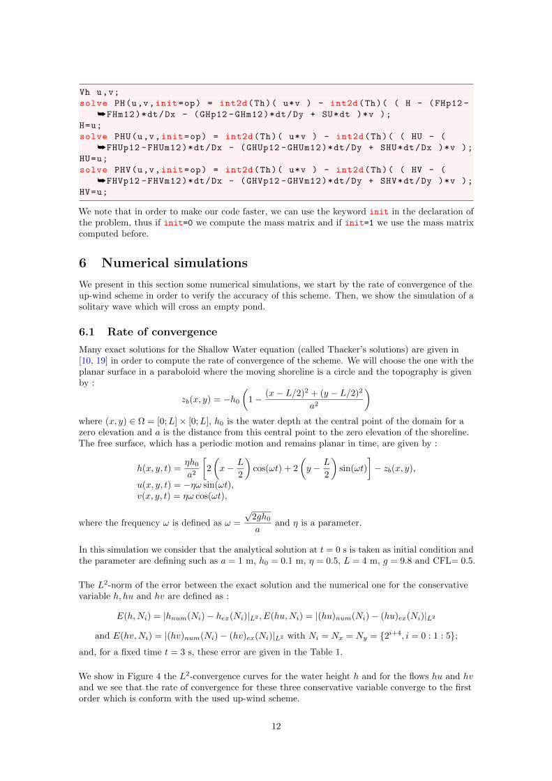
and E(hv,Ni) = |(hv)num(Ni)− (hv)ex(Ni)|L2 with Ni = Nx = Ny = 2i+4, i = 0 : 1 : 5;and, for a fixed time t = 3 s, these error are given in the Table 1.

We show in Figure 4 the L2-convergence curves for the water height h and for the flows hu and hvand we see that the rate of convergence for these three conservative variable converge to the firstorder which is conform with the used up-wind scheme.

12

We remind that the rate of convergence in space for u is :

r(•, Ni) =log (E(•, Ni−1)/E(•, Ni))

log (Ni/Ni−1),∀i = 0 : 1 : 5

Ni E(h,Ni) r(h,Ni) E(hu,Ni) r(hu,Ni) E(hv,Ni) r(hv,Ni)16 0.0278598 - 0.0212665 - 0.0253648 -32 0.0187917 0.5681 0.0145818 0.5444 0.0164372 0.625964 0.0116788 0.6862 0.00914136 0.6737 0.0101747 0.6920128 0.00686053 0.7675 0.00536215 0.7696 0.00599727 0.7626256 0.00382327 0.8435 0.00297793 0.8485 0.00334075 0.8441512 0.00204941 0.8996 0.00159311 0.9025 0.00177952 0.9087

Table 1: L2 norm of the error and the rate of convergence for h, hu and hv.

10−3

10−2

10−1

100

10−3

10−2

10−1

100

log (∆x)

log( ||Ψ

num−

Ψex||2 L

2

)

Order of accuracy in loglog scale for the Shallow Water equation

Ψ=h

Ψ=hu

Ψ=hv

order 1

Figure 4: Rate of convergence for the Shallow Water equations.

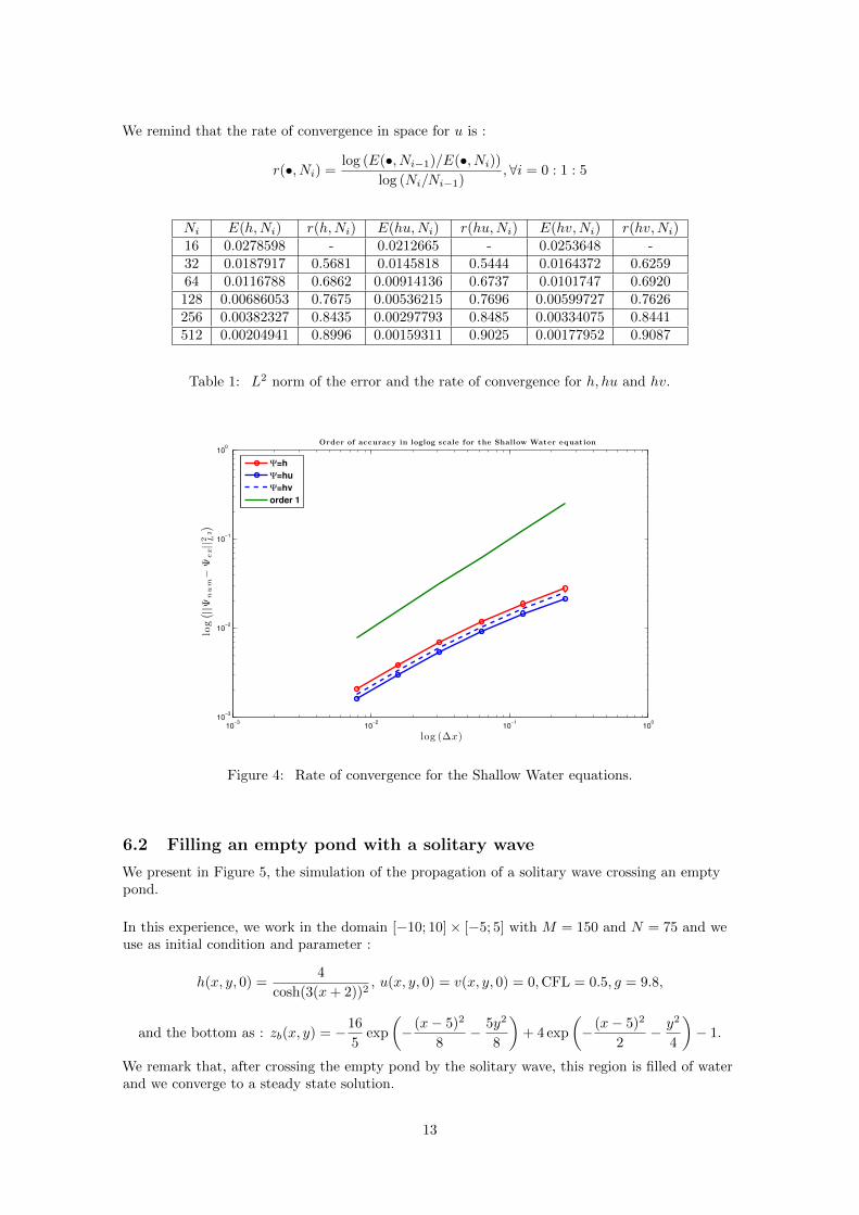
6.2 Filling an empty pond with a solitary wave

We present in Figure 5, the simulation of the propagation of a solitary wave crossing an emptypond.

In this experience, we work in the domain [−10; 10]× [−5; 5] with M = 150 and N = 75 and weuse as initial condition and parameter :

h(x, y, 0) =4

cosh(3(x+ 2))2, u(x, y, 0) = v(x, y, 0) = 0,CFL = 0.5, g = 9.8,

and the bottom as : zb(x, y) = −16

5exp

(− (x− 5)2

8− 5y2

8

)+ 4 exp

(− (x− 5)2

2− y2

4

)− 1.

We remark that, after crossing the empty pond by the solitary wave, this region is filled of waterand we converge to a steady state solution.

13

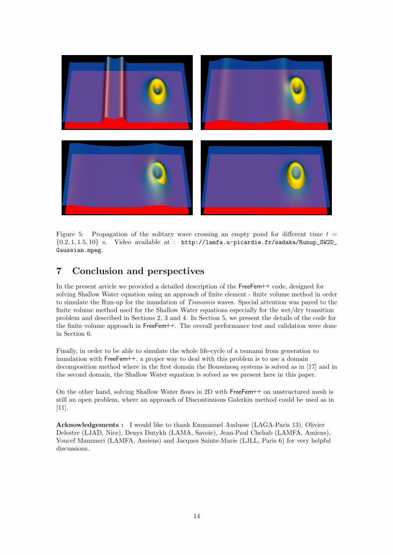
Figure 5: Propagation of the solitary wave crossing an empty pond for different time t =0.2, 1, 1.5, 10 s. Video available at : http://lamfa.u-picardie.fr/sadaka/Runup_SW2D_

Gaussian.mpeg.

7 Conclusion and perspectives

In the present article we provided a detailed description of the FreeFem++ code, designed forsolving Shallow Water equation using an approach of finite element - finite volume method in orderto simulate the Run-up for the inundation of Tsunamis waves. Special attention was payed to thefinite volume method used for the Shallow Water equations especially for the wet/dry transitionproblem and described in Sections 2, 3 and 4. In Section 5, we present the details of the code forthe finite volume approach in FreeFem++. The overall performance test and validation were donein Section 6.

Finally, in order to be able to simulate the whole life-cycle of a tsunami from generation toinundation with FreeFem++, a proper way to deal with this problem is to use a domaindecomposition method where in the first domain the Boussinesq systems is solved as in [17] and inthe second domain, the Shallow Water equation is solved as we present here in this paper.

On the other hand, solving Shallow Water flows in 2D with FreeFem++ on unstructured mesh isstill an open problem, where an approach of Discontinuous Galerkin method could be used as in[11].

Acknowledgements : I would like to thank Emmanuel Audusse (LAGA-Paris 13), OlivierDelestre (LJAD, Nice), Denys Dutykh (LAMA, Savoie), Jean-Paul Chehab (LAMFA, Amiens),Youcef Mammeri (LAMFA, Amiens) and Jacques Sainte-Marie (LJLL, Paris 6) for very helpfuldiscussions.

14

References

[1] Celine Acary-Robert, Didier Bresch and Denys Dutykh. Mathematical modeling ofpowder-snow avalanche flows. Studies in Applied Mathematics, 127(1), 38 - 66, 2011.

[2] Emmanuel Audusse. Modesitation hyperbolique et analyse numerique pour les ecoulementsen eaux peu profondes. These de l’Universite de Pierre et Marie Curie - Paris 6, 2004.

[3] Emmanuel Audusse and Marie-Odile Bristeau. A well-balanced positivity preserving”second-order” scheme for shallow water flows on unstructured meshes. JCP, Volume 206,Issue 1, Pages 311-333, 2005.

[4] Emmanuel Audusse, Christophe Chalons, Olivier Delestre, Nicole Goutal,Jacques Sainte-Marie, Jan Giesselmann and Georges Sadaka. Sediment transportmodeling relaxation schemes for Saint-Venant - Exner and three layer models. ProceedingsCEMRACS’11 (submit- ted), 2011.

[5] Alfredo Bermudez and Maria Elena Vazquez. Upwind methods for hyperbolicconservation laws with source terms. Computers & Fluids, 23(8) :1049 - 1071, 1994.

[6] Philippe Bonneton and Fabien Marche. A simple and efficient well-balanced model for2DH bore propagation and run-up over a sloping beach. Coastal Engineering, proceedings ofthe 30th International Conference, page 998-1010, 2006.

[7] Philippe Bonneton, Pierre Fabrie, Fabien Marche and Nicolas Seguin.Evaluationof well-balanced bore-capturing schemes for 2D wetting and drying processes. Int. J. Numer.Meth. Fluids, 53:867-894, 2007.

[8] Francois Bouchut, Anne Mangeney-Castelnau, Benoıt Perthame and Jean-Pierre Vilotte. A new model of Saint-Venant and Savage-Hutter type for gravity drivenshallow water flows. C. R. Math. Acad. Sci. Paris, 336, no.6, 531-536, 2003.

[9] Olivier Delestre. Simulation du ruissellement d’eau de pluie sur des surfaces agricoles.These de l’Universite d’Orleans, 2010.

[10] Olivier Delestre, Carine Lucas, Pierre-Antoine Ksinant, Frederic Darboux,Christian Laguerre, Thi Ngoc Tuoi Vo, Francois James and Stephane Cordier.SWASHES: a compilation of Shallow Water Analytic Solutions for Hydraulic and Environmen-tal Studies. HAL arXiv:1110.0288v3, 2012.

[11] Karim DjaDel, Alexandre Ern and Serge Piperno. A well-balanced Runge-Kutta Discontinuous Galerkin method for the Shallow Water Equations withflooding and drying. Int. J. Numer. Meth. Fluids, 58(1), 1-25, 2008.

[12] Barre de Saint-Venant. Theorie du mouvement non permanent des eaux, avec applicationaux crues des rivieres et a l’introduction des marees dans leur lit. Comptes Rendus des Seancesde l’Academie des Sciences. Paris. 73, 147-154, 237-240, 1871.

[13] Frederic Dias, Denys Dutykh and Raphael Poncet. The VOLNA code for thenumerical modeling of tsunami waves: generation, propagation and inundation. EuropeanJournal of Mechanics B/Fluids, 30(6), 598 - 615, 2011.

15

[14] Joshua M. Greenberg and A. Y. LeRoux. A well-balanced scheme for the numericalprocessing of source terms in hyperbolic equation. SIAM Journal on Numerical Analysis, 33:1-16, 1996.

[15] Ami Harten. High resolution schemes for hyperbolic conservation laws. J. Comp. Physics, 49,357–393, 1983.

[16] Mario Ricchiuto. Contributions to the development of residual discretization for hyperbolicconservation laws with application to shallow water flows. HDR dissertation, September 2011.

[17] Georges Sadaka. Etude mathematique et numerique d’equations d’ondes aquatiquesamorties. These de l’Universite de Picardie Jules Verne - Amiens, 2011.

[18] Denis Serre. Systemes hyperboliques de lois de conservation. Parties I et II., Diderot, Paris,1996.

[19] William Carlisle Thacker. Some exact solutions to the nonlinear shallow water waveequations. Journal of Fluid Mechanics, 107:499-508, 1981.

16