Embed Size (px)
Citation preview
Mathematical Programming manuscript No.(will be inserted by the editor)
R. H. Tutuncu, K. C. Toh, ·M. J. Todd
Solving semidefinite-quadratic-linear programsusing SDPT3 ?
Received: March 19, 2001 / Accepted: January 18, 2002Published online: October 9, 2002 – c©Springer Verlag 2002
Abstract. This paper discusses computational experiments with linear optimization problemsinvolving semidefinite, quadratic, and linear cone constraints (SQLPs). Many test problemsof this type are solved using a new release of SDPT3, a Matlab implementation of infeasibleprimal-dual path-following algorithms. The software developed by the authors uses Mehrotra-type predictor-corrector variants of interior-point methods and two types of search directions:the HKM and NT directions. A discussion of implementation details is provided and computa-tional results on problems from the SDPLIB and DIMACS Challenge collections are reported.
1. Introduction
Conic linear optimization problems can be expressed in the following standardform:
min 〈c, x〉s.t. 〈ak, x〉 = bk, k = 1, . . . ,m, (1)
x ∈ K
where K is a closed, convex pointed cone in a finite dimensional inner productspace endowed with an inner product 〈·, ·〉. By choosing K to be the semidefinite,quadratic (second-order), and linear cones respectively, one obtains the well-known special cases of semidefinite, second-order cone, and linear programmingproblems. Recent years have seen a dramatic increase in the number of subclassesof conic optimization problems that can be solved efficiently by interior-pointmethods. In addition to the ongoing theoretical work that derived convergenceguarantees and convergence rates for such algorithms, many groups of researchers
R. H. Tutuncu: Department of Mathematical Sciences, Carnegie Mellon University, Pittsburgh,PA 15213, USA. e-mail: [email protected]. Research supported in part by NSF throughgrant CCR-9875559.
K. C. Toh: Department of Mathematics, National University of Singapore, 10 Kent RidgeCrescent, Singapore 119260. e-mail: [email protected]. Research supported in partby the Singapore-MIT Alliance.
M. J. Todd: School of Operations Research and Industrial Engineering, Cornell University,Ithaca, New York 14853, USA. e-mail: [email protected]. Research supported in partby NSF through grant DMS-9805602 and ONR through grant N00014-96-1-0050.
Mathematics Subject Classification (1991): 90C05, 90C22
? Copyright (C) by Springer-Verlag. Mathematical Programming 95 (2003), 189–217.
2 R. H. Tutuncu, K. C. Toh,, M. J. Todd
have also implemented these algorithms and developed public domain softwarepackages that are capable of solving conic optimization problems of ever increas-ing size and diversity. This paper discusses the authors’ contribution to this effortthrough the development of the software SDPT3. Our earlier work on SDPT3 ispresented in [22,25].
The current version of SDPT3, version 3.0, can solve conic linear optimizationproblems with inclusion constraints for the cone of positive semidefinite matrices,the second-order cone, and/or the polyhedral cone of nonnegative vectors. Inother words, we allow K in (1) to be a Cartesian product of cones of positivesemidefinite matrices, second-order cones, and the nonnegative orthant. We usethe following standard form of such problems, henceforth called SQLP problems:
(P ) min∑ns
j=1〈csj , xs
j〉 +∑nq
i=1〈cqi , xq
i 〉 + 〈cl, xl〉
s.t.∑ns
j=1(Asj)
T svec(xsj) +
∑nq
i=1(Aqi )
T xqi + (Al)T xl = b,
xsj ∈ K
sjs ∀j, xq
i ∈ Kqiq ∀i, xl ∈ Knl
l .
Here, csj , xs
j are symmetric matrices of dimension sj and Ksjs is the cone of
positive semidefinite symmetric matrices of the same dimension. Similarly, cqi ,
xqi are vectors in IRqi and Kqi
q is the second-order cone defined by Kqiq :=
{x ∈ IRqi : x1 ≥ ‖x2:qi‖}. Finally, cl, xl are vectors of dimension nl andKnl
l is the cone IRnl+ . In the notation above, As
j denotes the sj × m matrixwith sj = sj(sj + 1)/2 whose columns are obtained using the svec opera-tor from m symmetric sj × sj constraint matrices corresponding to the jthsemidefinite block xs
j . (Here, for a symmetric matrix x of order s, svec(x) :=(x11,
√2x12, x22,
√2x13,
√2x23, x33, . . .)T ∈ IRs(s+1)/2, where the
√2 is to make
the operation an isometry.) The matrices Aqi ’s are qi×m dimensional constraint
matrices corresponding to the ith quadratic block xqi , and Al is the l × m di-
mensional constraint matrix corresponding to the linear block xl. The notation〈p, q〉 denotes the standard inner product in the appropriate space.
The software also solves the dual problem associated with the problem above:
(D) max bT ys.t. As
jy + zsj = cs
j , j = 1 . . . , ns,
Aqi y + zq
i = cqi , i = 1 . . . , nq,
Aly + zl = cl,
zsj ∈ K
sjs ∀j, zq
i ∈ Kqiq ∀i, zl ∈ Knl
l .
This package is written in Matlab version 5.3 and is compatible with Mat-lab version 6.0. It is available from the internet sites:
http://www.math.nus.edu.sg/~mattohkc/index.html
http://www.math.cmu.edu/~reha/sdpt3.html
This software package was originally developed to provide researchers insemidefinite programming with a collection of reasonably efficient and robust
Solving semidefinite-quadratic-linear programs using SDPT3 3
algorithms that can solve general SDPs with matrices of dimensions of the orderof a hundred. The current release, version 3.0, expands the family of problemssolvable by the software in two dimensions. First, this version is much fasterthan the previous release [25], especially on large sparse problems, and conse-quently can solve much larger problems. Second, the current release can alsodirectly solve problems that have second-order cone constraints — with the pre-vious version it was necessary to convert such constraints to semidefinite coneconstraints.
In this paper, the vector 2-norm and Frobenius norm are denoted by ‖ · ‖and ‖ · ‖F , respectively. In the next section, we discuss the algorithm used in thesoftware and several computational details. Section 3 describes the initial iteratesgenerated by our software while Section 4 briefly describes its options, someimplementation details, and its data storage scheme. In Section 5, we presentand comment on the results of our computational experiments with our softwareon problems from the SDPLIB and DIMACS libraries. Section 6 contains a shortconclusion.
2. A primal-dual infeasible-interior-point algorithm
The algorithm implemented in SDPT3 is a primal-dual interior-point algorithmthat uses the path-following paradigm. In each iteration, we first compute a pre-dictor search direction aimed at decreasing the duality gap as much as possible.After that, the algorithm generates a Mehrotra-type corrector step [14] withthe intention of keeping the iterates close to the central path. However, we donot impose any neighborhood restrictions on our iterates.1 Initial iterates neednot be feasible — the algorithm tries to achieve feasibility and optimality of itsiterates simultaneously.
It should be noted that our implementation allows the user to switch to aprimal-dual path-following algorithm that does not use corrector steps and sets acentering parameter to be used in such a framework. The choices we make on theparameters used by the algorithm are based on minimizing either the number ofiterations or the CPU time of the linear algebra involved in computing the Schurcomplement matrix and its Cholesky factorization. What follows is a pseudo-codefor the algorithm we implemented. Note that this description makes referencesto later parts of this section where many details related to the algorithm areexplained.
Algorithm IPC. Suppose we are given an initial iterate (x0, y0, z0) with x0, z0 strictlysatisfying all the conic constraints. Decide on the type of search direction to use. Set γ0 = 0.9.Choose a value for the parameter expon used in e.
For k = 0, 1, . . .
1 This strategy works well on most problems we tested. However, it should be noted thatthe occasional failure of the software on problems with poorly chosen initial iterates is likelydue to the lack of a neighborhood enforcement in the algorithm.
4 R. H. Tutuncu, K. C. Toh,, M. J. Todd
(Let the current and the next iterate be (x, y, z) and (x+, y+, z+) respectively. Also, let thecurrent and the next step-length parameter be denoted by γ and γ+ respectively.)
– Set µ = 〈x, z〉/n, and
relgap =〈x, z〉
1 + max(|〈c, x〉|, |bT y|), φ = max
( ‖rp‖1 + ‖b‖
,‖Rd‖
1 + ‖c‖
). (2)
Stop the iteration if the infeasibility measure φ and the relative duality gap (relgap) aresufficiently small.
– (Predictor step)Solve the linear system (10), with σ = 0 in the right-side vector (12). Denote the solutionof (4) by (δx, δy, δz). Let αp and βp be the step-lengths defined as in (33) and (34) with∆x, ∆z replaced by δx, δz, respectively.
– Take σ to be
σ = min
(1,
[ 〈x + αp δx, z + βp δz〉〈x, z〉
]e),
where the exponent e is chosen as follows:
e =
{max[expon, 3min(αp, βp)2] if µ > 10−6,
expon if µ ≤ 10−6.
– (Corrector step)
Solve the linear system (10) with Rc in the the right-hand side vector (12) replaced by
Rsc = svec [σµI −HP (smat(xs)smat(zs))−HP (smat(δxs)smat(δzs))]
Rqc = σµeq − TG(xq , zq)− TG(δxq , δzq)
Rlc = σµel − diag(xl)zl − diag(δxl)δzl.
Denote the solution of (4) by (∆x, ∆y, ∆z).– Update (x, y, z) to (x+, y+, z+) by
x+ = x + α ∆x, y+ = y + β ∆y, z+ = z + β ∆z,
where α and β are computed as in (33) and (34) with γ chosen to be γ = 0.9+0.09 min(αp, βp).– Update the step-length parameter by
γ+ = 0.9 + 0.09 min(α, β).
2.1. The search direction
To simplify discussion, we introduce the following notation, which is also consis-tent with the internal data representation in SDPT3:
As =
As1...
Asns
, Aq =
Aq1...
Aqnq
.
Similarly, we define
xs =
svec(xs1)
...svec(xs
ns)
, xq =
xq1...
xqnq
. (3)
Solving semidefinite-quadratic-linear programs using SDPT3 5
The vectors cs, zs, cq, and zq are defined analogously. We will use correspondingnotation for the search directions as well. Finally, let
AT =
As
Aq
Al
, x =
xs
xq
xl
, c =
cs
cq
cl
, z =
zs
zq
zl
,
and
n =ns∑
j=1
sj + nq + nl.
With the notations introduced above, the primal and dual equality constraintscan be represented respectively as
Ax = b, AT y + z = c.
In this paper, we assume that A has full row rank. However, the preprocessoption, when it is turned on, will correctly detect and remove dependent con-straints.
The main step at each iteration of our algorithms is the computation ofthe search direction (∆x,∆y,∆z) from the symmetrized Newton equation withrespect to an invertible block diagonal scaling matrix P for the semidefinite blockand a block scaling matrix G for the quadratic block. The matrices P and G areusually chosen as a function of the current iterate x, z and we will elaborate onspecific choices below. The search direction (∆x,∆y,∆z) is obtained from thefollowing system of equations:
AT ∆y + ∆z = Rd := c− z −AT y
A∆x = rp := b−Ax
Es∆xs + Fs∆zs = Rsc := svec (σµI −HP (smat(xs)smat(zs)))
Eq∆xq + Fq∆zq = Rqc := σµeq − TG(xq , zq)
El∆xl + F l∆zl = Rlc := σµel − ElF lel,
(4)
where µ = 〈x, z〉/n and σ is the centering parameter. The notation smat denotesthe inverse map of svec and both are to be interpreted as blockwise operators ifthe argument consists of blocks. Here HP is the symmetrization operator whoseaction on the jth semidefinite block is defined by
HPj: IRsj×sj −→ IRsj×sj
HPj (U) = 12
[PjUP−1
j + P−Tj UT PT
j
], (5)
with Pj the jth block of the block diagonal matrix P and Es and Fs are sym-metric block diagonal matrices whose jth blocks are given by
Esj = Pj ©∗ P−T
j zsj , Fs
j = Pjxsj ©∗ P−T
j , (6)
6 R. H. Tutuncu, K. C. Toh,, M. J. Todd
where R©∗ T is the symmetrized Kronecker product operation described in [22].In the quadratic block, eq denotes the blockwise identity vector, i.e.,
eq =
eq1...
eqnq
,
where eqj is the first unit vector in IRqj . Let the arrow operator defined in [3] be
denoted by Arw (·). Thus Arw (x) is a block diagonal matrix whose ith blockis
Arw(xi)
:= Arw(
xi0
xi1
):=(
xi0 xiT
1
xi1 xi
0Ini
).
Then the operator TG(xq, zq) is defined as follows:
TG(xq, zq) =
Arw (G1x
q1) (G−1
1 zq1)
...Arw
(Gnqx
qnq
)(G−1
nqzqnq
)
, (7)
where G is a symmetric block diagonal matrix that depends on x, z and Gi isthe ith block of G. The matrices Eq and Fq are block diagonal matrices whosethe ith blocks are given by
Eqi = Arw
(G−1
i zqi
)Gi, Fq
i = Arw (Gixqi ) G−1
i . (8)
In the linear block, el denotes the nl-dimensional vector of ones, and E l =diag(zl), F l = diag(xl).
For future reference, we partition the vectors Rd, ∆x, and ∆z in a manneranalogous to c, x, and z as follows:
Rd =
Rsd
Rqd
Rld
, ∆x =
∆xs
∆xq
∆xl
, ∆z =
∆zs
∆zq
∆zl
. (9)
Assuming that m = O(n), we compute the search direction via a Schurcomplement equation as follows (the reader is referred to [2] and [22] for details).First compute ∆y from the Schur complement equation
M∆y = h, (10)
where
M = (As)T (Es)−1FsAs + (Aq)T (Eq)−1FqAq + (Al)T (E l)−1F lAl (11)
h = rp − (As)T (Es)−1(Rsc −FsRs
d)− (Aq)T (Eq)−1(Rq
c −FqRqd) − (Al)T (E l)−1(Rl
c −F lRld). (12)

Solving semidefinite-quadratic-linear programs using SDPT3 7
Then compute ∆x and ∆z from the equations
∆z = Rd −AT ∆y (13)
∆xs = (Es)−1Rsc − (Es)−1Fs∆zs (14)
∆xq = (Eq)−1Rqc − (Eq)−1Fq∆zq (15)
∆xl = (E l)−1Rlc − (E l)−1F l∆zl. (16)
2.2. Two choices of search directions
We start by introducing some notation that we will use in the remainder of thispaper. For a given qi-dimensional vector xq
i , we let x0i denote its first component
and x1i denote its subvector consisting of the remaining entries, i.e.,[
x0i
x1i
]=
[(xq
i )1
(xqi )2:qi
]. (17)
We will use the same convention for zqi ,∆xq
i , etc. Also, we define the followingfunction from Kqi
q to IR+:
γ(xqi ) :=
√(x0
i )2 − 〈x1i , x1
i 〉. (18)
Finally, we use X and Z for smat(xs) and smat(zs), where the operation isapplied blockwise to form a block diagonal symmetric matrix of order
∑ns
j=1 sj .In the current release of this package, the user has two choices of scaling
operators parametrized by P and G, resulting in two different search directions:the HKM direction [10,12,16], and the NT direction [17]. See also Tsuchiya [26,27] for the second-order case.
(1) The HKM direction. This choice uses the scaling matrix P = Z1/2 for thesemidefinite blocks and a symmetric block diagonal scaling matrix G for thequadratic blocks where the ith block Gi is given by the following equation:
Gi =
z0i (z1
i )T
z1i γ(zq
i )I +z1i (z1
i )T
γ(zqi ) + z0
i
. (19)
(2) The NT direction. This choice uses the scaling matrix P = N−1 forthe semidefinite blocks, where N is a matrix such that D := NT ZN =N−1XN−T is a diagonal matrix [22], and G is a symmetric block diagonalmatrix whose ith block Gi is defined as follows. Let
ωi =
√γ(zq
i )γ(xq
i ), ξi =
[ξ0i
ξ1i
]=
[1ωi
z0i + ωix
0i
1ωi
z1i − ωix
1i
]. (20)
8 R. H. Tutuncu, K. C. Toh,, M. J. Todd
Then
Gi = ωi
t0i (t1i )T
t1i I +t1i (t
1i )
T
1 + t0i
, where
[t0i
t1i
]=
1γ(ξi)
[ξ0i
ξ1i
]. (21)
2.3. Computation of the search directions
The size and the density of the Schur complement matrix M defined in (10) isthe main determinant of the cost of each iteration in our algorithm. The densityof this matrix depends on two factors: (i) The density of the constraint coefficientmatrices As, Aq, and Al, and (ii) any additional fill-in introduced because of theterms (Es)−1Fs, (Eq)−1Fq, and (E l)−1F l in (10).
2.3.1. Semidefinite blocks For problems with semidefinite blocks, it appearsthat there is not much one can do about additional fill-in, since (Es)−1Fs isdense and structure-less for most problems. One can take advantage of sparsityin As in related computations, however, and we discussed some of these issues,such as blockwise computations, in our earlier papers [22,25].
The way we exploit sparsity of Asj in the computation of Ms
j := (Asj)
T (Esj )−1Fs
j Asj
basically follows the approach in [7]. We will not go into the details here but justbriefly highlight one issue that is often critical in cutting down the computationtime in forming Ms
j . Let Asj(:, k) be the kth column of As
j . In computing the kthcolumn of Ms
j , typically a matrix product of the form xsj smat(As
j(:, k)) (zsj )−1 or
wsj smat(As
j(:, k))wsj is required for the HKM direction or NT direction, respec-
tively. In many large SDP problems, the matrix smat(Asj(:, k)) is usually very
sparse, and it is important to store this matrix as a sparse matrix in Matlaband perform sparse-dense matrix-matrix multiplication in the matrix productsjust mentioned whenever possible. Also, entries of this product only need tobe computed if they contribute to an entry of M , i.e., if they correspond to anonzero entry of As
j(:, k′) for some k′.
2.3.2. Quadratic and linear blocks For linear blocks, (E l)−1F l is a diagonalmatrix and it does not introduce any additional fill-in. This matrix does, however,affect the conditioning of the Schur complement matrix and is a popular subjectof research in implementations of interior-point methods for linear programming.
From equation (11), it is easily shown that the contribution of the quadraticblocks to the matrix M is given by
Mq = (Aq)T (Eq)−1FqAq =nq∑i=1
(Aqi )
T (Eqi )−1Fq
i Aqi︸ ︷︷ ︸
Mqi
. (22)
Solving semidefinite-quadratic-linear programs using SDPT3 9
For the HKM direction, (Eq)−1Fq is a block diagonal matrix whose ith blockis given by
(Eqi )−1Fq
i = G−1i Arw (Gix
qi ) G−1
i
=1
γ2(zqi )
〈xqi , zq
i 〉
[−1 00 I
]+
[x0
i
x1i
][z0i
−z1i
]T
+
[z0i
−z1i
][x0
i
x1i
]T . (23)
(Note that Arw(G−1
i zqi
)= I.) Thus, we see that matrix (Eq
i )−1Fqi in Mq
i is thesum of a diagonal matrix and a rank-two symmetric matrix. Hence
Mqi =
〈xqi , zq
i 〉γ2(zq
i )(Aq
i )T JiA
qi + uq
i (vqi )T + vq
i (uqi )
T , (24)
where
Ji =
[−1 00 I
], uq
i = (Aqi )
T
[x0
i
x1i
], vq
i = (Aqi )
T
(1
γ2(zqi )
[z0i
−z1i
]). (25)
The appearance of the outer-product terms in the equation above is poten-tially alarming. If the vectors uq
i , vqi are dense, then even if Aq
i is sparse, thecorresponding matrix Mq
i , and hence the Schur complement matrix M , will bedense. A direct factorization of the resulting dense matrix will be very expensivefor even moderately high m.
The observed behavior of the density of the Schur complement matrix ontest problems depends largely on the particular problem structure. When theproblem has many small quadratic blocks, it is often the case that each blockappears in only a small fraction of the constraints. In this case, all Aq
i matricesare sparse and the vectors uq
i and vqi turn out to be sparse vectors for each i.
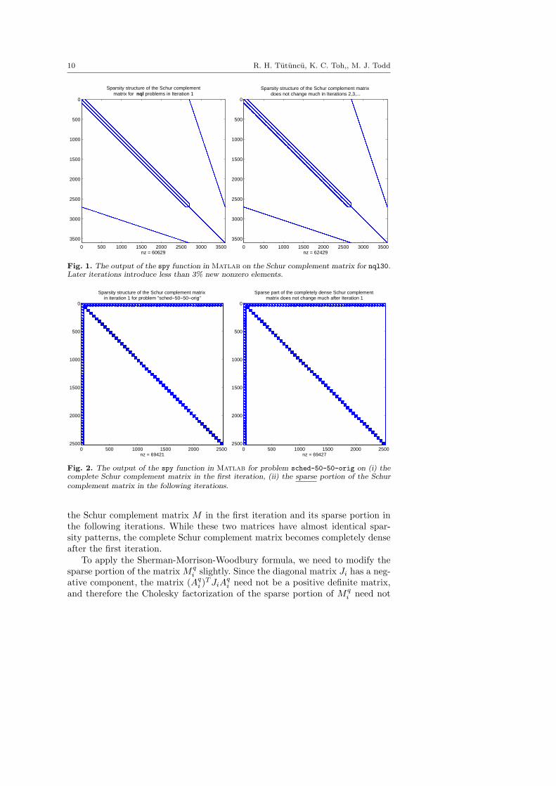
Consequently, the Schur complement matrix remains relatively sparse for theseproblems and it can be factorized directly and cheaply. In Figure 1, the densitystructures of the Schur complement matrices in the first and later iterations ofour algorithm applied to the the problem nql30 depict the situation and aretypical for all nql and qssp problems. Since we initially choose multiples ofunit vectors for our variables, all the nonzero elements of the Schur complementmatrix in the first iteration come from the nonzero elements of the constraintmatrices. Later iterations introduce fewer than 3% new nonzero elements.
The situation is drastically different for problems where one of the quadraticblocks, say the ith block, is large. For such problems the vectors uq
i , vqi are typ-
ically dense, and therefore, Mqi is likely be a dense matrix even if the data Aq
i
is sparse. However, observe that Mqi is a rank-two perturbation of a sparse ma-
trix when Aqi is sparse. In such a situation, it may be advantageous to use the
Sherman-Morrison-Woodbury update formula [9] when solving the Schur com-plement equation (10). This is a standard strategy used in linear programmingwhen there are dense columns in the constraint matrix and this is the approachwe used in our implementation of SDPT3. This approach helps tremendouslyon the scheduling problems from the DIMACS Challenge set. Figure 2 depicts
10 R. H. Tutuncu, K. C. Toh,, M. J. Todd
0 500 1000 1500 2000 2500 3000 3500
0
500
1000
1500
2000
2500
3000
3500
nz = 60629
Sparsity structure of the Schur complementmatrix for nql problems in Iteration 1
0 500 1000 1500 2000 2500 3000 3500
0
500
1000
1500
2000
2500
3000
3500
nz = 62429
Sparsity structure of the Schur complement matrix does not change much in Iterations 2,3,...
Fig. 1. The output of the spy function in Matlab on the Schur complement matrix for nql30.Later iterations introduce less than 3% new nonzero elements.
0 500 1000 1500 2000 2500
0
500
1000
1500
2000
2500
nz = 69421
Sparsity structure of the Schur complement matrix in iteration 1 for problem "sched−50−50−orig"
0 500 1000 1500 2000 2500
0
500
1000
1500
2000
2500
nz = 69427
Sparse part of the completely dense Schur complement matrix does not change much after Iteration 1
Fig. 2. The output of the spy function in Matlab for problem sched-50-50-orig on (i) thecomplete Schur complement matrix in the first iteration, (ii) the sparse portion of the Schur
complement matrix in the following iterations.
the Schur complement matrix M in the first iteration and its sparse portion inthe following iterations. While these two matrices have almost identical spar-sity patterns, the complete Schur complement matrix becomes completely denseafter the first iteration.
To apply the Sherman-Morrison-Woodbury formula, we need to modify thesparse portion of the matrix Mq
i slightly. Since the diagonal matrix Ji has a neg-ative component, the matrix (Aq
i )T JiA
qi need not be a positive definite matrix,
and therefore the Cholesky factorization of the sparse portion of Mqi need not
Solving semidefinite-quadratic-linear programs using SDPT3 11
exist. To overcome this problem, we use the following identity:
Mqi =
〈xqi , zq
i 〉γ2(zq
i )(Aq
i )T Aq
i + uqi (v
qi )T + vq
i (uqi )
T − 2〈xq
i , zqi 〉
γ2(zqi )
kikTi , (26)
where uqi and vq
i are as in (25) and
ki = (Aqi )
Teqi . (27)
Note that if Aqi is a large sparse matrix with a few dense rows, we also use the
Sherman-Morrison-Woodbury formula to handle the matrix (Aqi )
T Aqi in (26).
We end our discussion on the computation of the HKM direction with thefollowing formula that is needed in the computation of the right-hand-side vector(12):
(Eqi )−1(Rq
c)i =σµ
γ2(zqi )
[z0i
−z1i
]− xq
i . (28)
Just as for the HKM direction, we can obtain a very simple formula for(Eq
i )−1Fqi for the NT direction. By noting that Gix
qi = G−1
i zqi , it is easy to
see that the ith block (Eqi )−1Fq
i = G−2i , and a rather straightforward algebraic
manipulation gives the following identity:
(Eqi )−1Fq
i = G−2i =
1ω2
i
[−1 00 I
]+ 2
[t0i−t1i
][t0i−t1i
]T . (29)
For the NT direction, the formula in (28) also holds and we have:
Mqi =
1ω2
i
((Aq
i )T JiA
qi + 2uq
i (uqi )
T), with uq
i = (Aqi )
T
[t0i−t1i
]. (30)
We note that the identity (30) describing the NT direction was observed byother authors — see, e.g., [8]. The identities (23) and (24), however, appear to benew in the literature. It is straightforward, if a bit tedious, to verify these formu-las. In addition to simplifying the search direction computation, these identitiescan be used to provide a simple proof of the scale-invariance of the HKM searchdirection in second-order cone programming. In [27], Tsuchiya proves this resultand the scale-invariance of the NT direction using two-page arguments for eachproof. We refer the reader to [22] for a description of scale-invariance and providethe following simple and instructive proof:
Proposition 1. Consider a pure second-order cone programming problem (ns =0 and nl=0). The HKM and NT directions for this problem are scale-invariant.
12 R. H. Tutuncu, K. C. Toh,, M. J. Todd
Proof. The scaled problem is constructed as follows: Let Fi ∈ Gi denote ascaling matrix for block i where Gi is the automorphism group of the cone Kqi
q .For future reference, note that we have
FTi JiFi = Ji, FT
i Ji = JiF−1i , JiFi = F−T
i Ji, JiFTi = F−1
i Ji, (31)
where Ji = −Ji, and Ji is as in (25). Let F = diag[F1, . . . , Fnq] and define the
scaled quantities as follows:
Aq = F−1Aq, b = b, cq = F−1cq, xq = FT xq, y = y, zq = F−1zq.
Note that rp = rp and Rd = F−1Rd. First, we consider the HKM direction.We observe that γ2(zq
i ) = (zqi )T Jiz
qi = (zq
i )T F−Ti JiF
−1i zq
i = γ2(zqi ). Now, from
equation (24) and (31) it follows that each Mqi , and therefore Mq, is invariant
with respect to this automorphic scaling. Using (28), we see that h in (12)is also invariant. Now, if we denote the HKM search direction for the scaledproblem by (∆x
q, ∆y, ∆z
q) and the corresponding direction for the unscaled
problem by (∆xq,∆y,∆zq) we immediately obtain ∆y = ∆y from equation(10), ∆z
q= F−1∆zq from (13) and ∆x
q= FT ∆xq from (15) and (28). Thus,
the HKM direction for SOCP is scale-invariant.To prove the result for the NT direction, we first observe that γ(xq
i ) = γ(xqi )
and that ωi defined in (20) remains unchanged after scaling. The scaled equiva-lent of ξi defined in (20) is ξi = 1
ωizqi + ωiJix
qi = F−1
i ( 1ωi
zqi + ωiJix
qi ) = F−1
i ξi.Thus, with the scaled quantities, we obtain
ti =
[t0i
t1i
]= F−1
i
[t0i
t1i
].
Now, from equation (30) and (31) it follows that each Mqi , and therefore Mq,
is invariant with respect to this automorphic scaling. Continuing as above, weconclude that the NT direction for SOCP must be scale-invariant as well. ut
2.4. Step-length computation
Once a direction ∆x is computed, a full step will not be allowed if x+∆x violatesthe conic constraints. Thus, the next iterate must take the form x + α∆x for anappropriate choice of the step-length α. In this subsection, we discuss an efficientstrategy to compute the step-length α.
For semidefinite blocks, it is straightforward to verify that, for the jth block,the maximum allowed step-length that can be taken without violating the posi-tive semidefiniteness of the matrix xs
j + αsj∆xs
j is given as follows:
αsj =
−1
λmin((xsj)−1∆xs
j), if the minimum eigenvalue λmin is negative
∞ otherwise.(32)
Solving semidefinite-quadratic-linear programs using SDPT3 13
If the computation of eigenvalues necessary in αsj above becomes expensive, then
we resort to finding an approximation of αsj by estimating extreme eigenvalues
using Lanczos iterations [24]. This approach is quite accurate in general andrepresents a good trade-off between the effort versus quality of the resultingstepsizes.
For quadratic blocks, the largest step-length αqi that keeps the next iterate
feasible with respect to the kth quadratic cone can be computed as follows. Let
ai = γ2(∆xqi ), bi = 〈∆xq
i , −Jixqi 〉, ci = γ2(xq
i ),
where Ji is the matrix defined in (25) and let
di = b2i − aici.
We want the largest α with aiα2 + 2biα + ci > 0 for all smaller positive values.
This is given by
αqi =
−bi −
√di
aiif ai < 0 or bi < 0, ai ≤ b2
i /ci
−ci
2biif ai = 0, bi < 0
∞ otherwise.
For the linear block, the maximum allowed step-length αli for the hth com-
ponent is given by
αlh =
−xl
h
∆xlh
, if ∆xlh < 0
∞ otherwise.
Finally, an appropriate step-length α that can be taken in order for x + α∆x tosatisfy all the conic constraints takes the form
α = min(
1, γ min1≤j≤ns
αsj , γ min
1≤i≤nq
αqi , γ min
1≤h≤nl
αlh
), (33)
where γ (known as the step-length parameter) is typically chosen to be a numberslightly less than 1, for example as in the adaptive scheme shown in AlgorithmIPC, to ensure that the next iterate x + α∆x stays strictly in the interior of allthe cones.
For the dual direction ∆z, we let the analog of αsj , αq
i and αlh be βs
j , βqi
and βlh, respectively. Similar to the primal direction, the step-length that can be
taken by the dual direction ∆z is given by
β = min(
1, γ min1≤j≤ns
βsj , γ min
1≤i≤nq
βqi , γ min
1≤h≤nl
βlh
). (34)
14 R. H. Tutuncu, K. C. Toh,, M. J. Todd
2.5. Sherman-Morrison-Woodbury formula and iterative refinement
In this subsection, we discuss how we solve the Schur complement equation whenM is a low rank perturbation of a sparse matrix. As discussed in Section 2.3 suchsituations arise when the SQLP does not have a semidefinite block, but has largequadratic blocks or the constraint matrices Aq
i , Al have a small number of denserows. In such a case, the Schur complement matrix M can be written in the form
M = H + UV T (35)
where H is a sparse symmetric matrix and U, V have only few columns. If H isnon-singular, then by the Sherman-Morrison-Woodbury formula, the solution ofthe Schur complement equation is given by
∆y = h−H−1U(I + V T H−1U
)−1V T h, (36)
where h = H−1h.Computing ∆y via the Sherman-Morrison-Woodbury update formula above
is not always stable, and the computed solution for ∆y can be highly inaccu-rate when H is ill-conditioned. To overcome such a difficulty, we combine theSherman-Morrison-Woodbury update with iterative refinement [11]. It is notedin [11] that iterative refinement is beneficial even if the residuals are computedonly at the working precision. Our numerical experience with the SQLP prob-lems from the DIMACS Challenge set confirmed that iterative refinement veryoften does greatly improve the accuracy of the computed solution for ∆y via theSherman-Morrison-Woodbury formula. However, we must mention that iterativerefinement can occasionally fail to provide any significant improvement. We havenot yet incorporated a stable and efficient method for computing ∆y when Mhas the form (35), but note that Goldfarb and Scheinberg [8] discuss a stableproduct-form Cholesky factorization approach to this problem.
3. Initial iterates
Our algorithms can start with an infeasible starting point. However, the perfor-mance of these algorithms is quite sensitive to the choice of the initial iterate.As observed in [7], it is desirable to choose an initial iterate that at least hasthe same order of magnitude as an optimal solution of the SQLP. If a feasiblestarting point is not known, we recommend that the following initial iterate beused:
y0 = 0,
(xsj)
0 = ξsj Isj
, (zsj )
0 = ηsj Isj
, j = 1, . . . , ns,
(xqi )
0 = ξqi eq
i , (zqi )0 = ηq
i eqi , i = 1, . . . , nq,
(xl)0 = ξl el, (zl)0 = ηl el,
Solving semidefinite-quadratic-linear programs using SDPT3 15
where Isjis the identity matrix of order sj , and
ξsj = sj max1≤k≤m
1 + |bk|1 + ‖As
j(:, k)‖, ηs
j =1
√sj
[1 + max(max
k{‖As
j(:, k)‖}, ‖csj‖F )
],
ξqi =
√qi max
1≤k≤m
1 + |bk|1 + ‖Aq
i (:, k)‖, ηq
i =√
qi [1 + max(maxk{‖Aq
i (:, k)‖}, ‖cqi ‖)],
ξl = max1≤k≤m
1 + |bk|1 + ‖Al(:, k)‖
, ηl = 1 + max(maxk{‖Al(:, k)‖}, ‖cl‖),
where Asj(:, k) denotes the kth column of As
j , and Aqi (:, k) and Al
i(:, k) are definedsimilarly.
By multiplying the identity matrix Isiby the factors ξs
i and ηsi for the
semidefinite blocks, and similarly for the quadratic and linear blocks, the initialiterate has a better chance of having the appropriate order of magnitude.
The above iterate is the default in SDPT3, but other options are also avail-able.
4. Some implementation details
SDPT3 version 3.0 (henceforth denoted SDPT3-3.0) implements the infeasiblepath-following algorithms described in Section 2. It is designed to be fairly flex-ible in the strategies used, allowing either the HKM or the NT search direction,switching on or off scaling of the problem and/or the predictor-corrector scheme,giving a choice of step-length determination, etc. (However, as we describe inthe next section, the still available version 2.3 (denoted SDPT3-2.3) is moreflexible, allowing two more search directions as well as homogeneous self-dualalgorithms: we discuss below why these possibilities have been removed fromthe current version.) Details of these options can be found in the user’s guide[28], available from the web sites named in the introduction. The computationalresults given in the next section were all obtained with default settings, exceptthat we tested both search directions.
The output of SDPT3 is also flexible. Generally the output variables (X,y,Z)provide approximately optimal solutions, but if the output variable info(1) is1 the problem is suspected to be primal infeasible and (y,Z) is an approximatecertificate of infeasibility, with bTy = 1, Z in the appropriate cone, and ATy+ Zsmall, while if info(1) is 2 the problem is suspected to be dual infeasible and X isan approximate certificate of infeasibility, with 〈C, X〉 = −1, X in the appropriatecone, and A X small. In the case that an indication of infeasibility is given, thefinal iterates are still available to the user.
C Mex files used.
Our software uses a number of Mex routines generated from C programs writtento carry out certain operations for which Matlab is not efficient. In particu-lar, operations such as extracting selected elements of a matrix, and performing
16 R. H. Tutuncu, K. C. Toh,, M. J. Todd
arithmetic operations on these selected elements, are all done in C. As an exam-ple, the vectorization operation svec is coded in the C program mexsvec.c.
We also use a number of Mex routines generated from the Fortran programsfor sparse Cholesky factorization discussed in Section 5.1.
Cell array representation for problem data.
Our implementation SDPT3 exploits the block structure of the given SQLPproblem. In the internal representation of the problem data, we classify eachsemidefinite block into one of the following two types:
1. a dense or sparse matrix of dimension greater than or equal to 30;2. a sparse block-diagonal matrix consisting of numerous sub-blocks each of
dimension less than 30.
The reason for using the sparse matrix representation to handle the case when wehave numerous small diagonal blocks is that it is less efficient for Matlab to workwith a large number of cell array elements compared to working with a single cellarray element consisting of a large sparse block-diagonal matrix. Technically, noproblem will arise if one chooses to store the small blocks individually insteadof grouping them together as a sparse block-diagonal matrix.
For the quadratic part, we typically group all quadratic blocks (small orlarge) into a single block, though it is not mandatory to do so. If there are alarge number of small blocks, it is advisable to group them all together as asingle large block consisting of numerous small sub-blocks for the same reasonwe mentioned before.
Let L = ns + nq + 1. For each SQLP problem, the block structure of theproblem data is described by an L × 2 cell array named blk, The content ofeach of the elements of the cell arrays is given as follows. If the jth block is asemidefinite block consisting of a single block of size sj, then
blk{j,1} = ’s’ blk{j, 2} = [sj]
A{j} = [sj x m sparse]
C{j}, X{j}, Z{j} = [sj x sj double or sparse],
where sj = sj(sj + 1)/2.If the jth block is a semidefinite block consisting of numerous small sub-
blocks, say p of them, of dimensions sj1, sj2, . . . , sjp such that∑p
k=1 sjk = sj,then
blk{j,1} = ’s’ blk{j, 2} = [sj1 sj2 · · · sjp]A{j} = [sj x m sparse]
C{j}, X{j}, Z{j} = [sj x sj sparse] ,
where sj =∑p
k=1 sjk(sjk + 1)/2.The above storage scheme for the data matrix As
j associated with the semidef-inite blocks of the SQLP problem represents a departure from earlier versions ofour implementation, such as the one described in [25] and SDPT3-2.3. Previously,
Solving semidefinite-quadratic-linear programs using SDPT3 17
the semidefinite part of A was represented by an ns×m cell array, where A{j,k}corresponds to the kth constraint matrix associated with the jth semidefiniteblock, and it was stored as an individual matrix in either dense or sparse format.Now, we store all the constraint matrices associated with the jth semidefiniteblock in vectorized form as a single sj ×m matrix where the kth column of thismatrix corresponds to the kth constraint matrix. The data format we used inearlier versions of SDPT3 was more natural but, for the sake of computationalefficiency, we adopted our current data representation. The reason for such achange is again due to the fact that it is less efficient for Matlab to work witha single cell array with many cells. We also avoid explicit loops over the index k.In the next section, we will discuss the consequence of this modification in ourstorage scheme.
If the ith block is a quadratic block consisting of numerous sub-blocks, sayp of them, of dimensions qi1, qi2, . . . , qip such that
∑pk=1 qik = qi, then
blk{i,1} = ’q’ blk{i, 2} = [qi1 qi2 · · · qip]A{i} = [qi x m sparse]
C{i}, X{i}, Z{i} = [qi x 1 double or sparse].
If the ith block is the linear block, then
blk{i,1} = ’l’ blk{i, 2} = nl
A{i} = [nl x m sparse]
C{i}, X{i}, Z{i} = [nl x 1 double or sparse].
Caveats.
We should mention that “solving” SQLPs is more subtle than linear program-ming. For example, it is possible that both primal and dual problems are feasible,but their optimal values are not equal. Also, either problem may be infeasiblewithout there being a certificate of that fact (so-called weak infeasibility). Insuch cases, our software package is likely to terminate after some iterations withan indication of short step-length or lack of progress. Also, even if there is acertificate of infeasibility, our infeasible-interior-point methods may not find it.(However, in our limited testing on randomly generated strongly infeasible prob-lems, our algorithms have been quite successful in detecting infeasibility.)
5. Computational experiments
Here we describe the results of our computational testing of SDPT3, on problemsfrom the SDPLIB collection of Borchers [4] as well as the DIMACS Challengetest problems [19]. In both, we solve a selection of the problems; in the DIMACSproblems, these are selected as the more tractable problems, while our subset ofthe SDPLIB problems is more representative (but we cannot solve the largesttwo maxG problems). Since our algorithm is a primal-dual method storing the
18 R. H. Tutuncu, K. C. Toh,, M. J. Todd
Problem m SD SO L opt. obj. value
bm1 883 882 – – 23.43982copo14 1275 [14 x 14] – 364 0copo23 5820 [23 x 23] – 1771 0filter48-socp 969 48 49 931 1.41612901filtinf1 983 49 49 945 primal inf.hamming-7-5-6 1793 128 – – 42 2
3hamming-9-8 2305 512 – – 224hinf12 43 24 – – -0.0231 (?)hinf13 57 30 – – -44.38 (?)minphase 48 48 – – 5.98nb 123 – [793 x 3] 4 -0.05070309nb-L1 915 – [793 x 3] 797 -13.01227nb-L2 123 – [1637, 838 x 3] 4 -1.628972nb-L2-bessel 123 – [123, 838 x 3] 4 -0.102571nql30 3680 – [900 x 3] 3602 -0.9460nql60 14560 – [3600 x 3] 14402 -0.935423nql180 130080 – [32400 x 3] 129602 -0.927717nql30old 3601 – [900 x 3] 5560 -0.9460nql60old 14401 – [3600 x 3] 21920 -0.935423nql180old 129601 – [32400 x 3] 195360 -0.927717qssp30 3691 – [1891 x 4] 2 -6.496675qssp60 14581 – [7381 x 4] 2 -6.562696qssp180 130141 – [65341 x 4] 2 -6.639527qssp30old 5674 – [1891 x 4] 3600 -6.496675qssp60old 22144 – [7381 x 4] 14400 -6.562696qssp180old 196024 – [65341 x 4] 129600 -6.639527sched-50-50-orig 2527 – [2474, 3] 2502 26,673sched-50-50-scaled 2526 – 2475 2502 7.852038sched-100-50-orig 4844 – [4741, 3] 5002 181,889sched-100-50-scaled 4843 – 4742 5002 67.166281sched-100-100-orig 8338 – [8235, 3] 10002 717,367sched-100-100-scaled 8337 – 8236 10002 27.331457sched-200-100-orig 18087 – [17884, 3] 20002 141,360sched-200-100-scaled 18086 – 17885 20002 51.812471torusg3-8 512 512 – – 457.358179toruspm3-8-50 512 512 – – 527.808663truss5 208 [33 x 10, 1] – – 132.6356779truss8 496 [33 x 19, 1] – – 133.1145891
Table 1. Selected DIMACS Challenge Problems. SD, SO, and L stand for semidefinite, second-order, and linear blocks, respectively. Notation like [33 x 19] indicates that there were 33semidefinite blocks, each a symmetric matrix of order 19, etc.
primal iterate X, it cannot exploit common sparsity in C and the constraintmatrix as well as dual methods or nonlinear-programming based methods. Weare therefore unable to solve the largest problems.
All results given below were obtained on a Pentium III PC (800MHz) with1G of memory running Linux, using Matlab 6.0. The test problems are listedin Tables 1 and 2, along with their dimensions. We also list optimal objectivevalues of these problems that are reported in [19] and [4].
Solving semidefinite-quadratic-linear programs using SDPT3 19
Problem m semidefinite blocks linear block opt. obj. value
arch8 174 161 174 7.05698control7 666 [70, 35] – 20.6251control10 1326 [100, 50] – 38.533control11 1596 [110, 55] – 31.959gpp250-4 251 250 – -747.3gpp500-4 501 500 – -1567.02hinf15 91 37 – 25mcp250-1 250 250 – 317.2643mcp500-1 500 500 – 598.1485qap9 748 82 – -1410†
qap10 1021 101 – -1093†
ss30 132 294 132 20.2395theta3 1106 150 – 42.16698theta4 1949 200 – 50.32122theta5 3028 250 – 57.23231theta6 4375 300 – 63.47709truss7 86 [150 x 2, 1] – -90.0001truss8 496 [33 x 19, 1] – -133.1146equalG11 801 801 – 629.1553equalG51 1001 1001 – 4005.601equalG32 2001 2001 – N/AmaxG11 800 800 – 629.1648maxG51 1000 1000 – 4003.809†
maxG32 2000 2000 – 1567.640qpG11 800 1600 – 2448.659qpG112 800 800 800 2448.659qpG51 1000 2000 – 1181.000†
qpG512 1000 1000 1000 1181.000†
thetaG11 2401 801 – 400.00thetaG11n 1600 800 – 400.00thetaG51 6910 1001 – 349.00thetaG51n 5910 1000 – 349.00
Table 2. Selected SDPLIB Problems. Note that qpG112 is identical to qpG11 except thatthe structure of the semidefinite block is exposed as a sparse symmetric matrix of order 800and a diagonal block of the same order, which can be viewed as a linear block, and similarlyfor qpG512. Also, thetaG11n is a more compact formulation of thetaG11, and similarly forthetaG51n.† For some problems, we obtained the following alternative objective values that we believe tobe more accurate: qap9: -1409.8, qap10: -1092.4, equalG32: 1567.627, maxG51: 4006.256, qpG51:1181.800.
5.1. Cholesky factorization
Earlier versions of SDPT3 were intended for problems that always have semidef-inite cone constraints. As we indicated above, for such problems, the Schur com-plement matrix M in (11) is a dense matrix after the first iteration. To solve theassociated linear system (10), we first find a Cholesky factorization of M andthen solve two triangular systems. When M is dense, a reordering of the rowsand columns of M does not alter the efficiency of the Cholesky factorizationand specialized sparse Cholesky factorization routines are not useful. Therefore,earlier versions of SDPT3 (up to version 1.3) simply used Matlab’s chol rou-tine for Cholesky factorizations. For versions 2.1 and 2.2, we introduced our ownCholesky factorization routine mexchol that utilizes loop unrolling and provided
20 R. H. Tutuncu, K. C. Toh,, M. J. Todd
2-fold speed-ups on some architectures compared to Matlab’s chol routine.However, in newer versions of Matlab that use numerics libraries based onLAPACK, Matlab’s chol routine is more efficient than our Cholesky factoriza-tion routine mexchol for dense matrices. Thus, in SDPT3-3.0, we use Matlab’schol routine whenever M is dense. We also use Matlab’s chol in the updatedversion SDPT3-2.3 of our matrix-based code.
For the solution of most second-order cone programming problems in DI-MACS test set, however, Matlab’s chol routine is not competitive. This islargely due to the fact that the Schur complement matrix M is often sparse forSOCPs and LPs, and Matlab cannot sufficiently take advantage of this spar-sity. To solve such problems more efficiently we imported the sparse Choleskysolver in Yin Zhang’s LIPSOL [31], an interior-point code for linear programmingproblems. It should be noted that LIPSOL uses Fortran programs developedby Esmond Ng and Barry Peyton for sparse Cholesky factorization [18]. WhenSDPT3 uses LIPSOL’s Cholesky solver, it first generates a symbolic factoriza-tion of the Schur complement matrix to determine the pivot order by examiningthe sparsity structure of this matrix carefully. Then, this pivot order is re-usedin later iterations to compute the Cholesky factors. In contrast to the case oflinear programming, however, the sparsity structure of the Schur complementmatrix can change during the iterations for SOCP problems. If this happens, thepivot order has to be recomputed. We detect changes in the sparsity structureby monitoring the number of nonzero elements of the Schur complement matrix.Since the default initial iterates we use for an SOCP problem are unit vectorsbut subsequent iterates are not, there is always a change in the sparsity patternof M after the first iteration. After the second iteration, the sparsity patternremains unchanged for most problems, and only one more change occurs in asmall fraction of the test problems.
The effect of including a sparse Cholesky solver option for SOCP problemswas dramatic. We observed speed-ups up to two orders of magnitude. SDPT3-3.0automatically makes a choice between Matlab’s built-in chol routine and thesparse Cholesky solver based on the density of the Schur complement matrix.
5.2. Vectorized matrices vs. sparse matrices
The current release, SDPT3-3.0, of the code stores the constraint matrix in“vectorized” form as described in Sections 2 and 4. In the previous versions,and in SDPT3-2.3, A is a doubly subscripted cell array of symmetric matricesfor the semidefinite blocks, as we outlined at the end of the previous section.The result of the change is that much less storage is required for the constraintmatrix, and that we save a considerable amount of time in forming the Schurcomplement matrix M in (11) by avoiding loops over the index k. Operationsrelating to forming and factorizing the Schur complement and hence computingthe predictor search direction comprise much of the computational work formost problem classes, ranging from 25% for qpG11 up to 99% for the largertheta problems, the control problems, copo14, hamming-7-5-6, and the nb
Solving semidefinite-quadratic-linear programs using SDPT3 21
HKM NTProblem Itn err1 err3 err5 err6 time Itn err1 err3 err5 err6 time
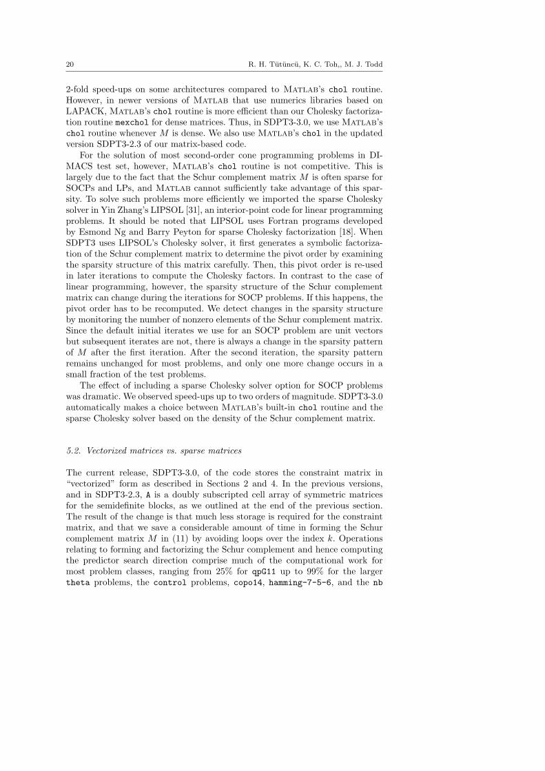
bm1 17 1-06 3-13 8-08 1-07 834 14 9-07 5-13 3-02 3-02 2891copo14 12 2-11 1-14 8-10 1-09 112 12 2-11 9-15 7-10 1-09 111copo23 16 3-12 6-14 2-10 4-10 4375 16 2-12 6-14 2-10 3-10 4343hamming-7-5-6 10 2-15 0 2-10 2-10 83 10 3-15 0 2-10 2-10 83hamming-9-8 12 8-15 0 2-10 2-10 341 12 7-15 0 2-10 2-10 646hinf12 42 2-08 5-10 -2-01 1-08 6 39 3-08 3-10 -2-01 5-08 7hinf13 24 8-05 1-12 -2-02 1-04 4 23 8-05 7-13 -2-02 9-05 5minphase 32 1-08 0 -2-04 3-08 6 37 2-08 0 -4-04 2-06 9torusg3-8 15 2-11 8-16 1-09 1-09 112 14 2-10 7-16 2-09 2-09 484toruspm3-8-50 13 2-11 6-16 3-09 3-09 93 14 5-11 6-16 2-10 2-10 470truss5 19 5-07 6-15 3-08 2-07 34 19 5-07 1-14 -9-08 3-08 37truss8 22 3-06 8-15 -2-06 2-07 306 21 2-06 1-14 -8-09 2-06 299
Table 3. Computational results on SDP problems in the DIMACS Challenge test set usingSDPT3-2.3. These were performed on a Pentium III PC (800MHz) with 1G of memory.
problems. Other significant parts are computing the corrector search direction(up to 75%) and computing step lengths (up to 60%).
While we now store the constraint matrix in vectorized form, the parts of theiterates X and Z corresponding to semidefinite blocks are still stored as matrices,since that is how the user wants to access them.
Results are given in Tables 3 through 6: Tables 3 and 4 give results on theDIMACS problems for both SDPT3-3.0 and SDPT3-2.3, while Tables 5 and 6give the comparable results for the SDPLIB problems. In all of these, the formatis the same. We give the number of iterations required, the time in seconds, andfour measures of the precision of the computed answer. These accuracy measuresare computed as follows:
err1 =‖Ax− b‖
1 + max |bk|,
err3 =‖AT y + z − c‖
1 + max |c|,
err5 =〈c, x〉 − bT y
1 + |〈c, x〉|+ |bT y|,
err6 =〈x, z〉
1 + |〈c, x〉|+ |bT y|.
In err3 the norm is subordinate to the inner product and the maximum is takenover all components of c. These measures are almost identical to the measuresreported by Mittelmann in [15], except that he uses ‖b‖1 instead of max |bk| inerr1, and similarly ‖c‖1 instead of max |c| in err3. Mittelmann also reports coneviolation measures err2 and err4 which are always zero for our iterates.
In general, both versions of our codes solved all problems without second-order cone constraints to reasonable accuracy (in terms of all measures) usingeither of the search directions. SDPT3-3.0 had difficulty obtaining high accuracysolutions to several DIMACS problems involving second-order cone constraints.
22 R. H. Tutuncu, K. C. Toh,, M. J. Todd
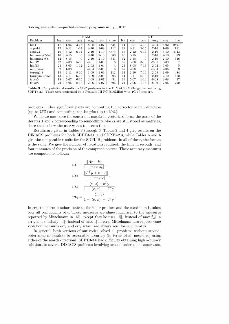
HKM NTProblem Itn err1 err3 err5 err6 time Itn err1 err3 err5 err6 time
bm1 18 4-07 8-12 1-07 1-07 811 16 1-08 5-13 1-05 1-05 2758copo14 15 1-10 6-15 -1-09 8-10 40 13 6-11 6-15 9-09 7-09 36copo23 17 2-09 1-14 8-08 5-10 1805 16 8-10 1-14 2-08 5-09 1695hamming-7-5-6 10 2-15 9-15 9-11 9-11 66 10 2-15 9-15 9-11 9-11 68hamming-9-8 11 5-15 9-14 4-09 4-09 212 11 5-15 8-14 4-09 4-09 418hinf12 42 2-08 4-10 -2-01 1-08 5 39 2-08 2-10 -2-01 6-09 5hinf13 23 9-05 8-13 -2-02 3-05 4 22 1-04 9-13 -2-02 6-06 4minphase 32 8-09 3-12 -2-04 1-08 5 37 2-08 7-13 -5-04 3-06 7torusg3-8 15 2-11 7-16 3-10 3-10 89 14 2-10 7-16 3-09 3-09 407toruspm3-8-50 14 2-11 6-16 2-09 2-09 84 15 4-11 6-16 7-10 7-10 432truss5 16 4-07 8-15 -3-10 1-07 9 16 4-07 8-15 -1-07 3-08 10truss8 15 3-06 8-15 -3-06 1-07 44 14 2-06 1-14 5-07 2-06 47
filter48-socp 38 1-06 9-14 1-05 1-06 51 45 1-06 8-14 1-05 1-06 60filtinf1 27 3-05 4-12 2-01 4-01 38 27 3-05 2-11 4-01 7-01 39nb 15 1-05 2-09 2-04 2-04 42 14 1-05 1-08 2-04 2-04 31nb-L1 16 7-05 4-09 2-05 1-05 73 16 2-04 9-11 1-06 9-07 59nb-L2 12 2-09 1-11 6-09 6-09 57 11 4-09 1-08 5-07 5-07 45nb-L2-bessel 13 8-06 4-12 9-07 5-08 39 11 3-07 2-09 6-07 7-07 26nql30 13 6-08 5-09 2-05 4-05 11 16 2-06 3-11 -5-06 1-06 12nql60 13 4-07 1-08 4-05 1-04 63 15 3-06 2-10 -2-05 9-06 57nql180 15 1-05 3-08 7-05 1-03 5622 16 7-05 4-10 -3-03 6-05 3235nql30old 12 5-05 2-08 -7-05 1-04 12 12 5-05 2-08 -8-05 1-04 12nql60old 13 1-04 7-09 -8-04 1-04 87 13 9-05 5-08 -4-04 5-04 75nql180old 9 9-04 3-05 -5-02 2-01 4015 10 1-03 8-06 -3-01 8-02 2742qssp30 21 7-08 1-09 7-07 8-07 24 18 3-07 2-11 -1-07 3-08 17qssp60 21 5-05 2-09 6-05 2-05 154 20 3-06 1-11 3-06 1-07 108qssp180 24 3-04 1-08 8-04 2-04 17714 25 3-05 4-12 7-05 4-08 9790qssp30old 11 3-04 4-05 5-02 6-02 58 12 5-04 6-05 3-02 4-02 60qssp60old 11 4-04 2-04 1-01 2-01 397 12 4-04 4-04 1-01 2-01 382sched-50-50-orig 28 7-04 3-09 -9-05 6-06 21 29 2-04 3-07 -1-05 7-06 20sched-50-50-scaled 23 1-04 4-15 2-05 3-05 18 22 6-05 4-15 1-06 7-06 16sched-100-50-orig 39 6-03 3-11 -8-04 2-06 63 33 6-03 2-11 8-04 5-07 50sched-100-50-scaled 26 8-04 9-13 1-04 1-04 44 22 7-04 1-09 3-04 3-04 35sched-100-100-orig 33 5-02 1-10 -2-02 4-07 102 50 5-01 3-10 1-00 1-07 136sched-100-100-scaled 19 4-02 1-14 -4-03 3-06 65 17 3-02 1-14 -2-03 1-02 55sched-200-100-orig 41 6-03 3-09 -4-03 3-06 348 39 6-03 1-08 -5-03 4-06 309sched-200-100-scaled 27 3-03 6-09 -8-04 7-04 247 25 3-03 7-10 -1-03 3-04 216
Table 4. Computational results on DIMACS Challenge problems using SDPT3-3.0. Thesewere performed on a Pentium III PC (800MHz) with 1G of memory.
We comment on some of these problems in detail in Section 5.6. We note thaton two problems, our codes terminated with an indication that X and Z were notboth positive definite: qpG11 (version 2.3, NT only) and sched-100-100-orig(version 3.0, NT only). However, this is a conservative test designed to stop ifnumerical difficulties are imminent. Using SeDuMi’s eigK.m routine to check theiterates, it was found that in both cases both variables were feasible in the conicconstraints.
The objective values of the optimal solutions generated by our codes matchthe optimal objective values listed in Tables 1 and 2 in most cases. Exceptions,however, are not limited to the problems where our codes had accuracy prob-lems. In particular, for problems bm1, torusg3-8, qap9, qap10, maxG51, andqpG51 SDPT3 generates accurate solutions whose optimal objective values dif-
Solving semidefinite-quadratic-linear programs using SDPT3 23
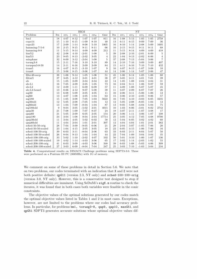
HKM NTProblem Itn err1 err3 err5 err6 time Itn err1 err3 err5 err6 time
arch8 19 9-10 5-13 2-09 2-09 55 23 1-08 5-13 4-08 4-08 74control7 23 7-07 2-09 1-07 8-07 149 22 4-07 2-09 1-06 2-06 156control10 24 6-07 5-09 1-06 3-06 709 24 1-06 6-09 -1-06 8-07 802control11 24 1-06 6-09 -3-06 4-07 1108 24 1-06 6-09 -1-06 1-06 1245gpp250-4 15 3-08 5-14 -9-09 4-09 28 13 7-06 2-13 1-05 2-05 62gpp500-4 15 3-08 2-14 4-09 5-09 169 13 7-08 3-14 2-05 2-05 501hinf15 24 9-05 2-12 -4-02 2-05 7 23 1-04 1-12 -4-02 2-04 8mcp250-1 13 2-11 5-16 4-09 4-09 14 15 7-12 4-16 9-10 9-10 55mcp500-1 14 1-11 5-16 8-10 8-10 79 15 2-11 5-16 4-09 4-09 416qap9 15 4-08 3-13 -2-05 1-08 19 15 5-08 3-13 -3-05 1-08 20qap10 14 4-08 3-13 -6-05 1-08 34 14 4-08 4-13 -6-05 5-09 36ss30 19 2-09 2-13 5-09 5-09 113 24 1-08 2-13 6-08 6-08 242theta3 14 3-11 6-15 1-09 1-09 40 14 2-10 6-15 4-10 2-10 45theta4 15 2-10 8-15 2-09 2-09 160 15 4-10 8-15 4-10 2-10 175theta5 15 2-10 1-14 2-09 2-09 475 14 4-10 1-14 5-09 5-09 483theta6 15 5-10 1-14 -2-10 4-10 1224 15 5-10 1-14 1-10 7-10 1302truss7 23 3-06 2-13 -5-06 4-07 6 22 4-06 2-13 -1-05 2-08 8truss8 22 3-06 8-15 -2-06 2-07 306 21 2-06 8-15 -8-09 2-06 299
equalG11 18 4-11 3-16 4-10 4-10 776 16 1-08 3-16 2-06 2-06 2451equalG51 20 8-09 4-16 -8-11 2-10 1586 20 5-08 5-16 2-08 2-08 5648equalG32 19 1-10 2-16 2-09 2-09 10170 15 4-07 2-16 9-05 9-05 33618maxG11 14 2-11 8-16 2-09 2-09 292 14 4-11 7-16 1-09 1-09 1540maxG51 16 1-11 4-16 2-09 2-09 951 16 9-11 3-16 3-10 3-10 4171maxG32 15 1-10 1-15 2-09 2-09 3726 15 2-10 1-15 6-10 6-10 24957qpG11 14 1-11 0 4-09 4-09 1429 15 2-11 0 4-09 4-09 6789qpG112 15 2-11 0 4-10 4-10 337 15 6-11 0 4-10 4-10 1693qpG51 21 6-11 0 4-09 4-09 4518 24 1-09 0 4-09 2-08 19817qpG512 17 2-10 0 4-09 4-09 965 25 9-11 0 2-09 2-09 6677thetaG11 20 3-09 8-14 -5-10 2-10 1196 17 8-09 5-15 1-09 3-09 2699thetaG11n 15 4-12 0 2-09 2-09 786 15 4-12 0 1-09 1-09 2240thetaG51 33 4-08 7-13 4-09 4-09 18992 30 7-09 8-14 2-08 2-08 23851thetaG51n 19 2-09 2-14 -1-09 1-08 5159 22 5-09 3-14 -2-09 7-10 10415
Table 5. Computational results on SDPLIB problems using SDPT3-2.3. These were performedon a Pentium III PC (800MHz) with 1G of memory.
fer from previously published optimal objective values which we believe to beincorrect. We also provide an accurate optimal objective value for equalG32which was previously unavailable. Finally, we note that some of the listed opti-mal objective values in Table 1 contain sign errors, see the caption for Table 1for details.
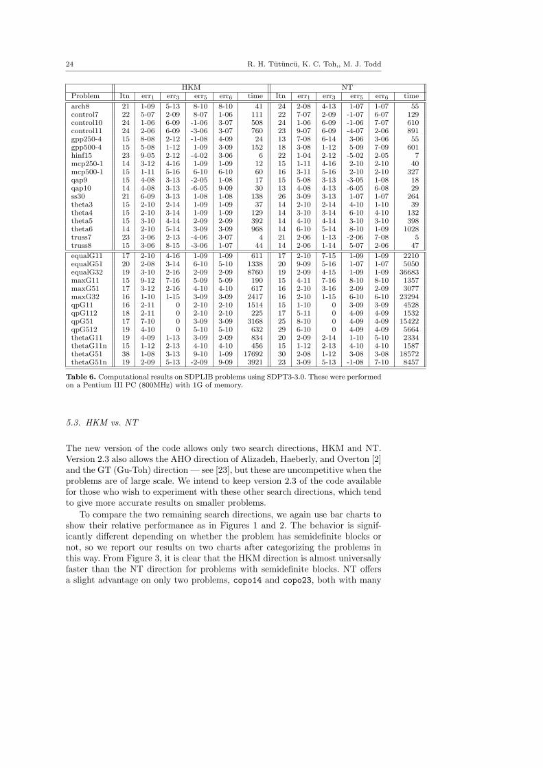
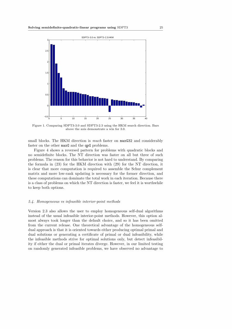
To compare the two codes in terms of time, we consider only the problemsthat both codes could solve, and omit the simplest problems with times under20 seconds (the hinf problems, minphase, and truss5 and truss7). For theremaining problems, we compute the ratio of the times taken by the two codes,take its logarithm to base 2, and then plot the results in decreasing order ofabsolute values. The results are shown in Figures 1 and 2 for the HKM and NTsearch directions. A bar of height 1 indicates that SDPT3-3.0 was 2 times fasterthan SDPT3-2.3, of −1 the reverse, and of 3 that SDPT3-3.0 was 8 times faster.Note that the new version using vectorized matrices is almost uniformly fasterand often at least 50% faster using either direction.
24 R. H. Tutuncu, K. C. Toh,, M. J. Todd
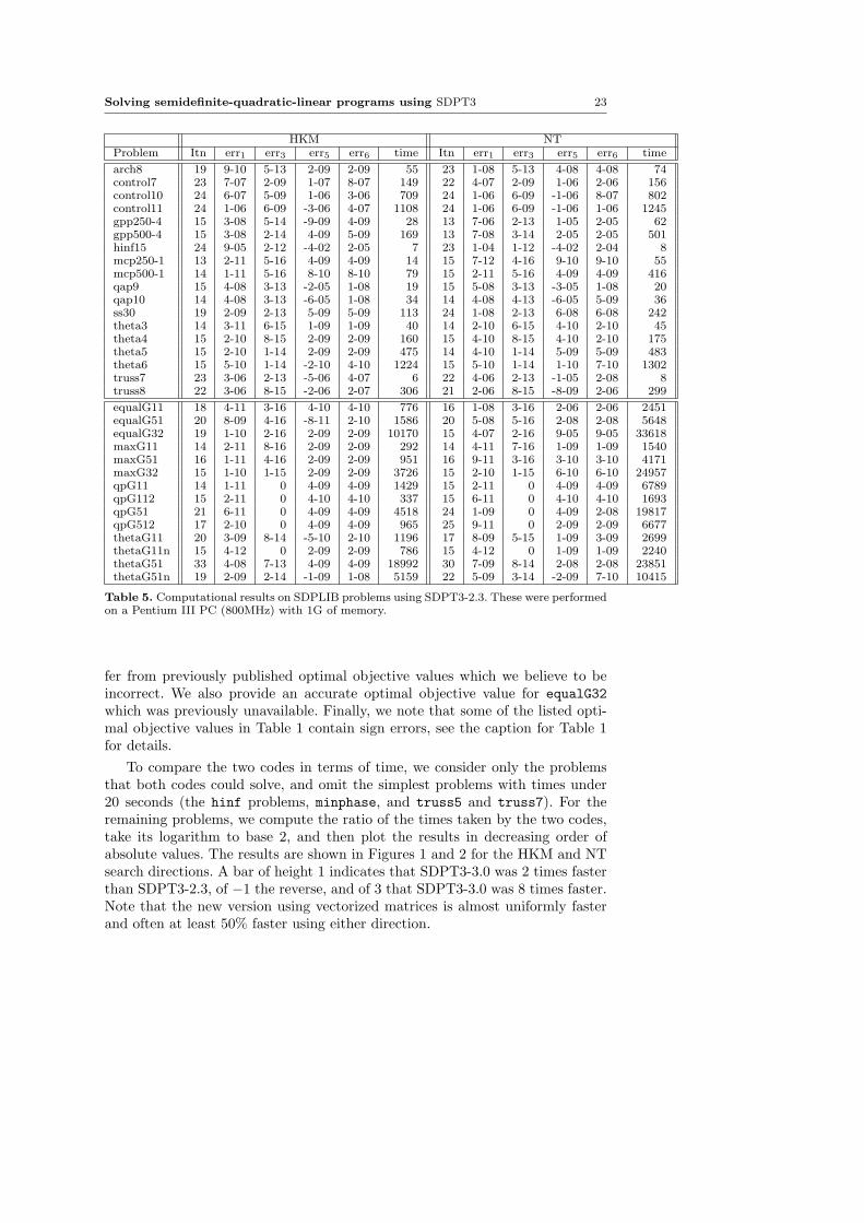
HKM NTProblem Itn err1 err3 err5 err6 time Itn err1 err3 err5 err6 time
arch8 21 1-09 5-13 8-10 8-10 41 24 2-08 4-13 1-07 1-07 55control7 22 5-07 2-09 8-07 1-06 111 22 7-07 2-09 -1-07 6-07 129control10 24 1-06 6-09 -1-06 3-07 508 24 1-06 6-09 -1-06 7-07 610control11 24 2-06 6-09 -3-06 3-07 760 23 9-07 6-09 -4-07 2-06 891gpp250-4 15 8-08 2-12 -1-08 4-09 24 13 7-08 6-14 3-06 3-06 55gpp500-4 15 5-08 1-12 1-09 3-09 152 18 3-08 1-12 5-09 7-09 601hinf15 23 9-05 2-12 -4-02 3-06 6 22 1-04 2-12 -5-02 2-05 7mcp250-1 14 3-12 4-16 1-09 1-09 12 15 1-11 4-16 2-10 2-10 40mcp500-1 15 1-11 5-16 6-10 6-10 60 16 3-11 5-16 2-10 2-10 327qap9 15 4-08 3-13 -2-05 1-08 17 15 5-08 3-13 -3-05 1-08 18qap10 14 4-08 3-13 -6-05 9-09 30 13 4-08 4-13 -6-05 6-08 29ss30 21 6-09 3-13 1-08 1-08 138 26 3-09 3-13 1-07 1-07 264theta3 15 2-10 2-14 1-09 1-09 37 14 2-10 2-14 4-10 1-10 39theta4 15 2-10 3-14 1-09 1-09 129 14 3-10 3-14 6-10 4-10 132theta5 15 3-10 4-14 2-09 2-09 392 14 4-10 4-14 3-10 3-10 398theta6 14 2-10 5-14 3-09 3-09 968 14 6-10 5-14 8-10 1-09 1028truss7 23 3-06 2-13 -4-06 3-07 4 21 2-06 1-13 -2-06 7-08 5truss8 15 3-06 8-15 -3-06 1-07 44 14 2-06 1-14 5-07 2-06 47
equalG11 17 2-10 4-16 1-09 1-09 611 17 2-10 7-15 1-09 1-09 2210equalG51 20 2-08 3-14 6-10 5-10 1338 20 9-09 5-16 1-07 1-07 5050equalG32 19 3-10 2-16 2-09 2-09 8760 19 2-09 4-15 1-09 1-09 36683maxG11 15 9-12 7-16 5-09 5-09 190 15 4-11 7-16 8-10 8-10 1357maxG51 17 3-12 2-16 4-10 4-10 617 16 2-10 3-16 2-09 2-09 3077maxG32 16 1-10 1-15 3-09 3-09 2417 16 2-10 1-15 6-10 6-10 23294qpG11 16 2-11 0 2-10 2-10 1514 15 1-10 0 3-09 3-09 4528qpG112 18 2-11 0 2-10 2-10 225 17 5-11 0 4-09 4-09 1532qpG51 17 7-10 0 3-09 3-09 3168 25 8-10 0 4-09 4-09 15422qpG512 19 4-10 0 5-10 5-10 632 29 6-10 0 4-09 4-09 5664thetaG11 19 4-09 1-13 3-09 2-09 834 20 2-09 2-14 1-10 5-10 2334thetaG11n 15 1-12 2-13 4-10 4-10 456 15 1-12 2-13 4-10 4-10 1587thetaG51 38 1-08 3-13 9-10 1-09 17692 30 2-08 1-12 3-08 3-08 18572thetaG51n 19 2-09 5-13 -2-09 9-09 3921 23 3-09 5-13 -1-08 7-10 8457
Table 6. Computational results on SDPLIB problems using SDPT3-3.0. These were performedon a Pentium III PC (800MHz) with 1G of memory.
5.3. HKM vs. NT
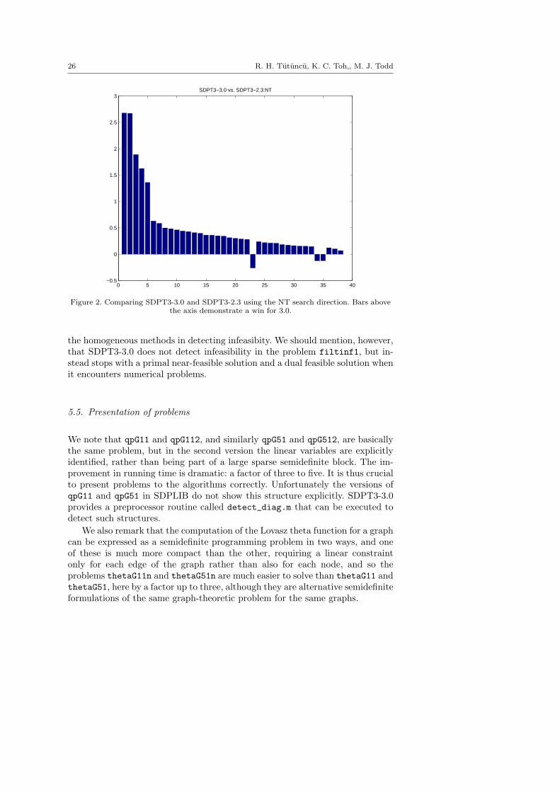
The new version of the code allows only two search directions, HKM and NT.Version 2.3 also allows the AHO direction of Alizadeh, Haeberly, and Overton [2]and the GT (Gu-Toh) direction — see [23], but these are uncompetitive when theproblems are of large scale. We intend to keep version 2.3 of the code availablefor those who wish to experiment with these other search directions, which tendto give more accurate results on smaller problems.
To compare the two remaining search directions, we again use bar charts toshow their relative performance as in Figures 1 and 2. The behavior is signif-icantly different depending on whether the problem has semidefinite blocks ornot, so we report our results on two charts after categorizing the problems inthis way. From Figure 3, it is clear that the HKM direction is almost universallyfaster than the NT direction for problems with semidefinite blocks. NT offersa slight advantage on only two problems, copo14 and copo23, both with many
Solving semidefinite-quadratic-linear programs using SDPT3 25
0 5 10 15 20 25 30 35 40−0.5
0
0.5
1
1.5
2
2.5
3SDPT3−3.0 vs. SDPT3−2.3:HKM
Figure 1. Comparing SDPT3-3.0 and SDPT3-2.3 using the HKM search direction. Barsabove the axis demonstrate a win for 3.0.
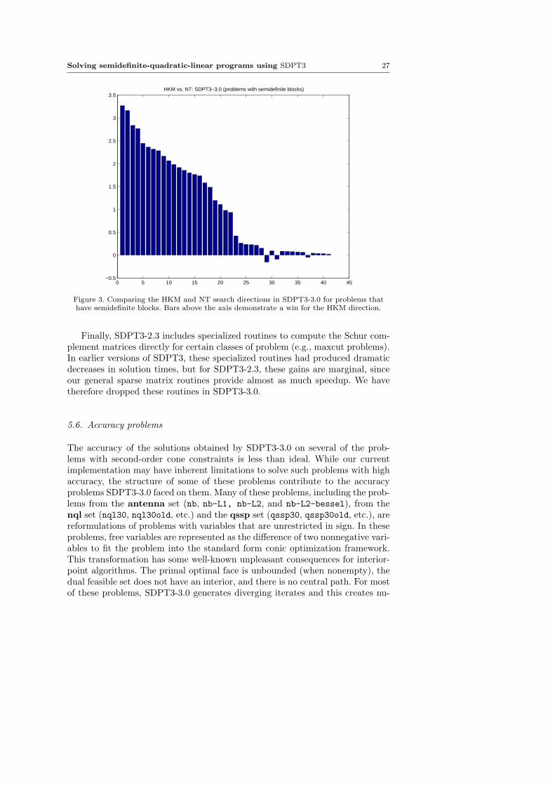
small blocks. The HKM direction is much faster on maxG32 and considerablyfaster on the other maxG and the qpG problems.
Figure 4 shows a reversed pattern for problems with quadratic blocks andno semidefinite blocks. The NT direction was faster on all but three of suchproblems. The reason for this behavior is not hard to understand. By comparingthe formula in (23) for the HKM direction with (29) for the NT direction, itis clear that more computation is required to assemble the Schur complementmatrix and more low-rank updating is necessary for the former direction, andthese computations can dominate the total work in each iteration. Because thereis a class of problems on which the NT direction is faster, we feel it is worthwhileto keep both options.
5.4. Homogeneous vs infeasible interior-point methods
Version 2.3 also allows the user to employ homogeneous self-dual algorithmsinstead of the usual infeasible interior-point methods. However, this option al-most always took longer than the default choice, and so it has been omittedfrom the current release. One theoretical advantage of the homogeneous self-dual approach is that it is oriented towards either producing optimal primal anddual solutions or generating a certificate of primal or dual infeasibility, whilethe infeasible methods strive for optimal solutions only, but detect infeasibil-ity if either the dual or primal iterates diverge. However, in our limited testingon randomly generated infeasible problems, we have observed no advantage to
26 R. H. Tutuncu, K. C. Toh,, M. J. Todd
0 5 10 15 20 25 30 35 40−0.5
0
0.5
1
1.5
2
2.5
3SDPT3−3.0 vs. SDPT3−2.3:NT
Figure 2. Comparing SDPT3-3.0 and SDPT3-2.3 using the NT search direction. Bars abovethe axis demonstrate a win for 3.0.
the homogeneous methods in detecting infeasibity. We should mention, however,that SDPT3-3.0 does not detect infeasibility in the problem filtinf1, but in-stead stops with a primal near-feasible solution and a dual feasible solution whenit encounters numerical problems.
5.5. Presentation of problems
We note that qpG11 and qpG112, and similarly qpG51 and qpG512, are basicallythe same problem, but in the second version the linear variables are explicitlyidentified, rather than being part of a large sparse semidefinite block. The im-provement in running time is dramatic: a factor of three to five. It is thus crucialto present problems to the algorithms correctly. Unfortunately the versions ofqpG11 and qpG51 in SDPLIB do not show this structure explicitly. SDPT3-3.0provides a preprocessor routine called detect_diag.m that can be executed todetect such structures.
We also remark that the computation of the Lovasz theta function for a graphcan be expressed as a semidefinite programming problem in two ways, and oneof these is much more compact than the other, requiring a linear constraintonly for each edge of the graph rather than also for each node, and so theproblems thetaG11n and thetaG51n are much easier to solve than thetaG11 andthetaG51, here by a factor up to three, although they are alternative semidefiniteformulations of the same graph-theoretic problem for the same graphs.
Solving semidefinite-quadratic-linear programs using SDPT3 27
0 5 10 15 20 25 30 35 40 45−0.5
0
0.5
1
1.5
2
2.5
3
3.5HKM vs. NT: SDPT3−3.0 (problems with semidefinite blocks)
Figure 3. Comparing the HKM and NT search directions in SDPT3-3.0 for problems thathave semidefinite blocks. Bars above the axis demonstrate a win for the HKM direction.
Finally, SDPT3-2.3 includes specialized routines to compute the Schur com-plement matrices directly for certain classes of problem (e.g., maxcut problems).In earlier versions of SDPT3, these specialized routines had produced dramaticdecreases in solution times, but for SDPT3-2.3, these gains are marginal, sinceour general sparse matrix routines provide almost as much speedup. We havetherefore dropped these routines in SDPT3-3.0.
5.6. Accuracy problems
The accuracy of the solutions obtained by SDPT3-3.0 on several of the prob-lems with second-order cone constraints is less than ideal. While our currentimplementation may have inherent limitations to solve such problems with highaccuracy, the structure of some of these problems contribute to the accuracyproblems SDPT3-3.0 faced on them. Many of these problems, including the prob-lems from the antenna set (nb, nb-L1, nb-L2, and nb-L2-bessel), from thenql set (nql30, nql30old, etc.) and the qssp set (qssp30, qssp30old, etc.), arereformulations of problems with variables that are unrestricted in sign. In theseproblems, free variables are represented as the difference of two nonnegative vari-ables to fit the problem into the standard form conic optimization framework.This transformation has some well-known unpleasant consequences for interior-point algorithms. The primal optimal face is unbounded (when nonempty), thedual feasible set does not have an interior, and there is no central path. For mostof these problems, SDPT3-3.0 generates diverging iterates and this creates nu-
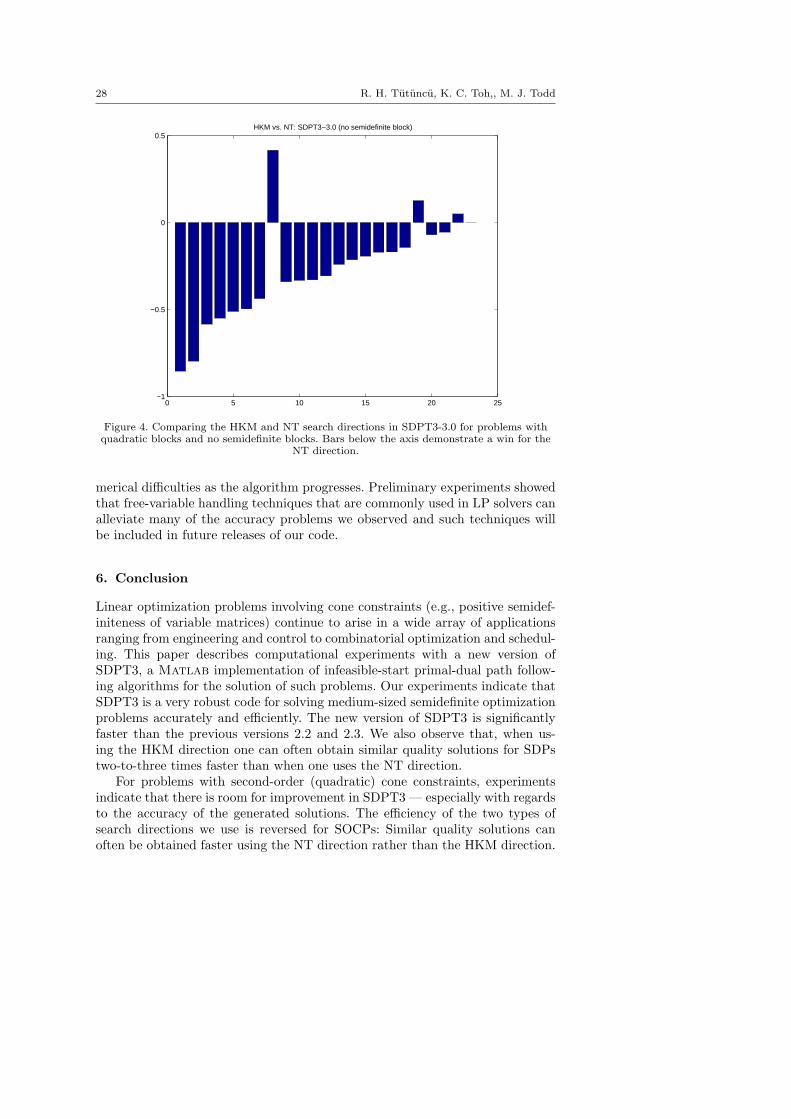
28 R. H. Tutuncu, K. C. Toh,, M. J. Todd
0 5 10 15 20 25−1
−0.5
0
0.5HKM vs. NT: SDPT3−3.0 (no semidefinite block)
Figure 4. Comparing the HKM and NT search directions in SDPT3-3.0 for problems withquadratic blocks and no semidefinite blocks. Bars below the axis demonstrate a win for the
NT direction.
merical difficulties as the algorithm progresses. Preliminary experiments showedthat free-variable handling techniques that are commonly used in LP solvers canalleviate many of the accuracy problems we observed and such techniques willbe included in future releases of our code.
6. Conclusion
Linear optimization problems involving cone constraints (e.g., positive semidef-initeness of variable matrices) continue to arise in a wide array of applicationsranging from engineering and control to combinatorial optimization and schedul-ing. This paper describes computational experiments with a new version ofSDPT3, a Matlab implementation of infeasible-start primal-dual path follow-ing algorithms for the solution of such problems. Our experiments indicate thatSDPT3 is a very robust code for solving medium-sized semidefinite optimizationproblems accurately and efficiently. The new version of SDPT3 is significantlyfaster than the previous versions 2.2 and 2.3. We also observe that, when us-ing the HKM direction one can often obtain similar quality solutions for SDPstwo-to-three times faster than when one uses the NT direction.
For problems with second-order (quadratic) cone constraints, experimentsindicate that there is room for improvement in SDPT3 — especially with regardsto the accuracy of the generated solutions. The efficiency of the two types ofsearch directions we use is reversed for SOCPs: Similar quality solutions canoften be obtained faster using the NT direction rather than the HKM direction.
Solving semidefinite-quadratic-linear programs using SDPT3 29
Overall, SDPT3 finds its niche as an efficient high-quality solver for mediumsized semidefinite optimization problems.
References
1. F. Alizadeh, Interior point methods in semidefinite programming with applications tocombinatorial optimization, SIAM J. Optim., 5 (1995), pp. 13–51.
2. F. Alizadeh, J.-P.A. Haeberly, and M.L. Overton, Primal-dual interior-point methods forsemidefinite programming: convergence results, stability and numerical results, SIAM J.Optim., 8 (1998), pp. 746–768.
3. F. Alizadeh, J.-P.A. Haeberly, M.V. Nayakkankuppam, M.L. Overton, and S. Schmieta,SDPPACK user’s guide, Technical Report, Computer Science Department, NYU, NewYork, June 1997.
4. B. Borchers, SDPLIB 1.2, a library of semidefinite programming test problems, Op-tim. Methods Softw., 11 & 12 (1999), pp. 683–690. Available at http://www.nmt.edu/~borchers/sdplib.html.
5. B. Borchers, CSDP, a C library for semidefinite programming, Optim. Methods Softw.,11 & 12 (1999), pp. 613–623. Available at http://www.nmt.edu/~borchers/csdp.html.
6. K. Fujisawa, M. Kojima, and K. Nakata, Exploiting sparsity in primal-dual interior-pointmethod for semidefinite programming, Math. Program., 79 (1997), pp. 235–253.
7. K. Fujisawa, M. Kojima, and K. Nakata, SDPA (semidefinite programming algo-rithm) — user’s manual, Research Report, Department of Mathematical and Com-puting Science, Tokyo Institute of Technology, Tokyo. Available via anonymous ftp atftp.is.titech.ac.jp in pub/OpRes/software/SDPA.
8. D. Goldfarb, and K. Scheinberg, A product-form Cholesky factorization implementationof an interior-point method for second order cone programming, preprint.
9. G.H. Golub, and C.F. Van Loan, Matrix Computations, 2nd ed., (Johns Hopkins UniversityPress, Baltimore, MD, 1989)
10. C. Helmberg, F. Rendl, R. Vanderbei and H. Wolkowicz, An interior-point method forsemidefinite programming, SIAM J. Optim., 6 (1996), pp. 342–361.
11. N.J. Higham, Accuracy and Stability of Numerical Algorithms, (SIAM, Philadelphia, 1996)12. M. Kojima, S. Shindoh, and S. Hara, Interior-point methods for the monotone linear
complementarity problem in symmetric matrices, SIAM J. Optim., 7 (1997), pp. 86–125.13. The MathWorks, Inc., Using MATLAB, (The MathWorks, Inc., Natick, MA, 1997)14. S. Mehrotra, On the implementation of a primal-dual interior point method, SIAM J.
Optim., 2 (1992), pp. 575–601.15. H.D. Mittelmann, An independent benchmarking of SDP and SOCP solvers, Math. Pro-
gram., this issue.16. R.D.C. Monteiro, Primal-dual path-following algorithms for semidefinite programming,
SIAM J. Optim., 7 (1997), pp. 663–678.17. Yu. Nesterov and M. J. Todd, Self-scaled barriers and interior-point methods in convex
programming, Math. Oper. Res., 22 (1997), pp. 1–42.18. E.G. Ng and B.W. Peyton, Block sparse Cholesky algorithms on advanced uniprocessor
computers, SIAM J. Sci. Comput., 14 (1993), pp. 1034–1056.19. G. Pataki and S. Schmieta, The DIMACS library of mixed semidefinite-quadratic-linear
programs. Available at http://dimacs.rutgers.edu/Challenges/Seventh/Instances.20. F.A. Potra and R. Sheng, On homogeneous interior-point algorithms for semidefinite
programming, Optim. Methods Softw. 9 (1998), pp. 161–184.21. J.F. Sturm, Using SeDuMi 1.02, a Matlab toolbox for optimization over symmetric cones,
Optim. Methods Softw., 11 & 12 (1999), pp. 625–653.22. M.J. Todd, K.C. Toh, R.H. Tutuncu, On the Nesterov-Todd direction in semidefinite
programming, SIAM J. Optim., 8 (1998), pp. 769–796.23. K. C. Toh, Some new search directions for primal-dual interior point methods in semidef-
inite programming, SIAM J. Optim., 11 (2000), pp. 223–242.24. K.C. Toh, A note on the calculation of step-lengths in interior-point methods for semidef-
inite programming, Comput. Optim. Appl., 21 (2002), pp. 301–310.25. K.C. Toh, M.J. Todd, R.H. Tutuncu, SDPT3 — a Matlab software package for semidefi-
nite programming, Optim. Methods Softw., 11 & 12 (1999), pp. 545-581.

30 Solving SQLPs using SDPT3
26. T. Tsuchiya, A polynomial primal-dual path-following algorithm for second-order coneprogramming, Technical Report, The Institute of Statistical Mathematics, Minato-Ku,Tokyo, October 1997.
27. T. Tsuchiya, A convergence analysis of the scaling-invariant primal-dual path-followingalgorithms for second-order cone programming, Optim. Methods Softw., 11 & 12 (1999),pp. 141–182.
28. R.H. Tutuncu, K.C. Toh, M.J. Todd, SDPT3 — a Matlab software pack-age for semidefinite-quadratic-linear programming, version 3.0. Available athttp://www.math.nus.edu.sg/~mattohkc/.
29. L. Vandenberghe and S. Boyd, Semidefinite programming, SIAM Rev., 38 (1996), pp.49–95.
30. L. Vandenberghe and S. Boyd, User’s guide to SP: software for semidefinite program-ming, Information Systems Laboratory, Stanford University, November 1994. Availablevia anonymous ftp at isl.stanford.edu in pub/boyd/semidef prog. Beta version.
31. Y. Zhang, Solving large-scale linear programs by interior-point methods under the Matlabenvironment, Optim. Methods Softw., 10 (1998), pp. 1–31.


![sdpt3r: Semidefinite Quadratic Linear Programming …...problem is finding the maximum cut of a graph. Let G = [V,E] be a graph with vertices V and edges E. A cut of the graph G](https://img.pdfslide.us/doc/110x75/5f1ccc20ec51d613822dabf7/sdpt3r-semideinite-quadratic-linear-programming-problem-is-inding-the-maximum.jpg)