SOLVING PROBLEMS BY SEARCHING

In which we see how an agent can find a sequence of actions that achieves its

goals.

Content

1. Problem-solving agents

2. Examples

3. Search for solutions

4. Search strategies

5. Specialties

6. Summary

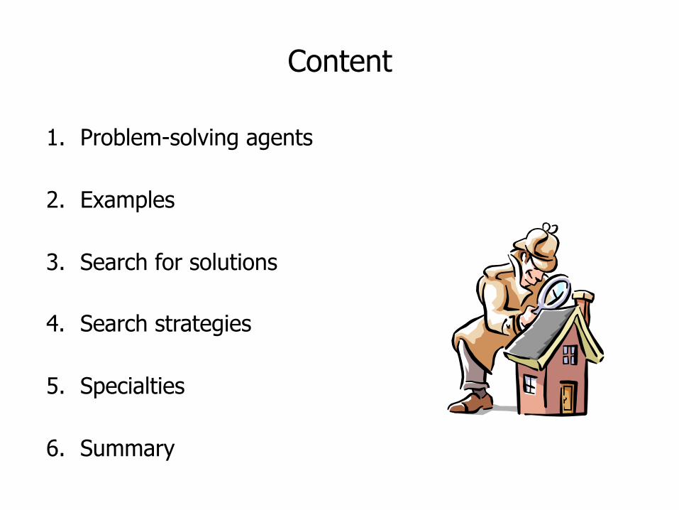
1. Problem-solving agents

All problem-solving agents are abstract – World state: specification of every aspect of reality – Problem state: only problem-relevant aspects

Vacuum cleaning robot (world state)

Vacuum cleaning robot (problem state)

3

4

Problem-solving agents

• Problem-solving agents is a special kind of goal-based agent.

• Tasks: – How to define a problem? – Problem type of formulation depends on available knowledge. – Problems, solutions, what is this?

• Six different search strategies.

5

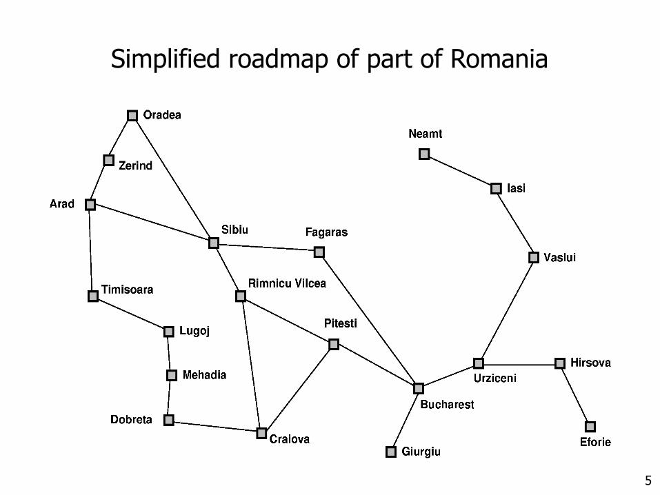
Simplified roadmap of part of Romania

6

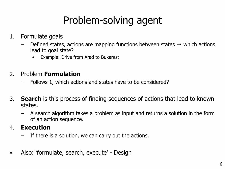
Problem-solving agent1. Formulate goals

– Defined states, actions are mapping functions between states → which actions lead to goal state? • Example: Drive from Arad to Bukarest

2. Problem Formulation – Follows 1, which actions and states have to be considered?

3. Search is this process of finding sequences of actions that lead to known states. – A search algorithm takes a problem as input and returns a solution in the form

of an action sequence.

4. Execution – If there is a solution, we can carry out the actions.

• Also: ‘formulate, search, execute’ - Design

7

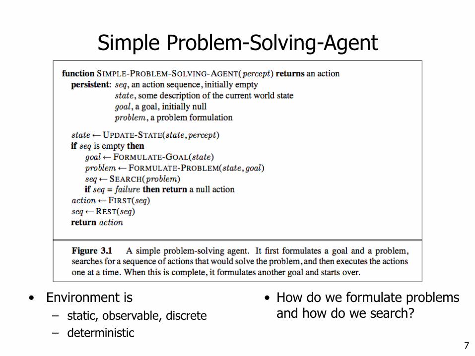
Simple Problem-Solving-Agent

• How do we formulate problems and how do we search?

• Environment is – static, observable, discrete – deterministic

8

Well-defined problems and solutions• Problems and solutions:

– Initial state – Possible actions available to the agent, e.g. successor function.

State space: the set of all states reachable from the initial state. A path in the state space is a sequence of states connected by a sequence of actions.

– Goal test: • Simple check: actual state = goal. • Abstract property rather than an explicitly enumerated set of states (e.g.

chess). – A path cost function that assigns a numeric cost to each path

• Initial state, set of actions. goal test and path cost functions together define a problem.

• Solution – Path from initial state to goal.

9

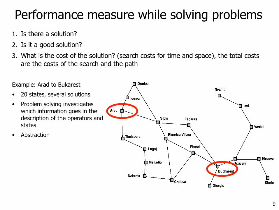
Performance measure while solving problems1. Is there a solution?

2. Is it a good solution?

3. What is the cost of the solution? (search costs for time and space), the total costs are the costs of the search and the path

Example: Arad to Bukarest

• 20 states, several solutions

• Problem solving investigates which information goes in the description of the operators and states

• Abstraction

10

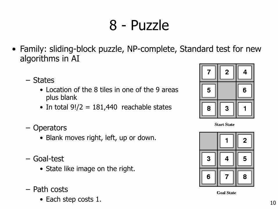
8 - Puzzle • Family: sliding-block puzzle, NP-complete, Standard test for new

algorithms in AI

– States • Location of the 8 tiles in one of the 9 areas

plus blank • In total 9!/2 = 181,440 reachable states

– Operators • Blank moves right, left, up or down.

– Goal-test • State like image on the right.

– Path costs • Each step costs 1.

11

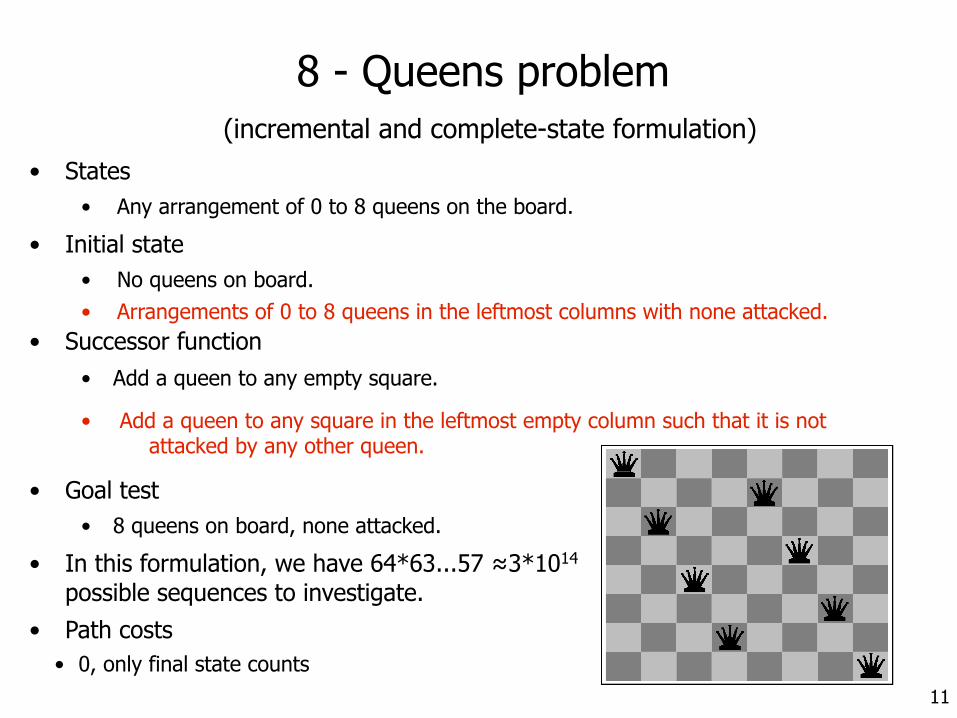
8 - Queens problem (incremental and complete-state formulation)

• States • Any arrangement of 0 to 8 queens on the board.

• Initial state • No queens on board.

• Successor function • Add a queen to any empty square.

• Goal test • 8 queens on board, none attacked.

• In this formulation, we have 64*63...57 ≈3*1014

possible sequences to investigate. • Path costs

• 0, only final state counts

• Arrangements of 0 to 8 queens in the leftmost columns with none attacked.

• Add a queen to any square in the leftmost empty column such that it is not attacked by any other queen.

12

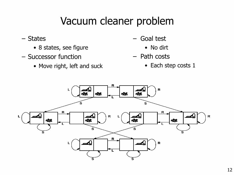
Vacuum cleaner problem– States

• 8 states, see figure

– Successor function • Move right, left and suck

– Goal test • No dirt

– Path costs • Each step costs 1

13

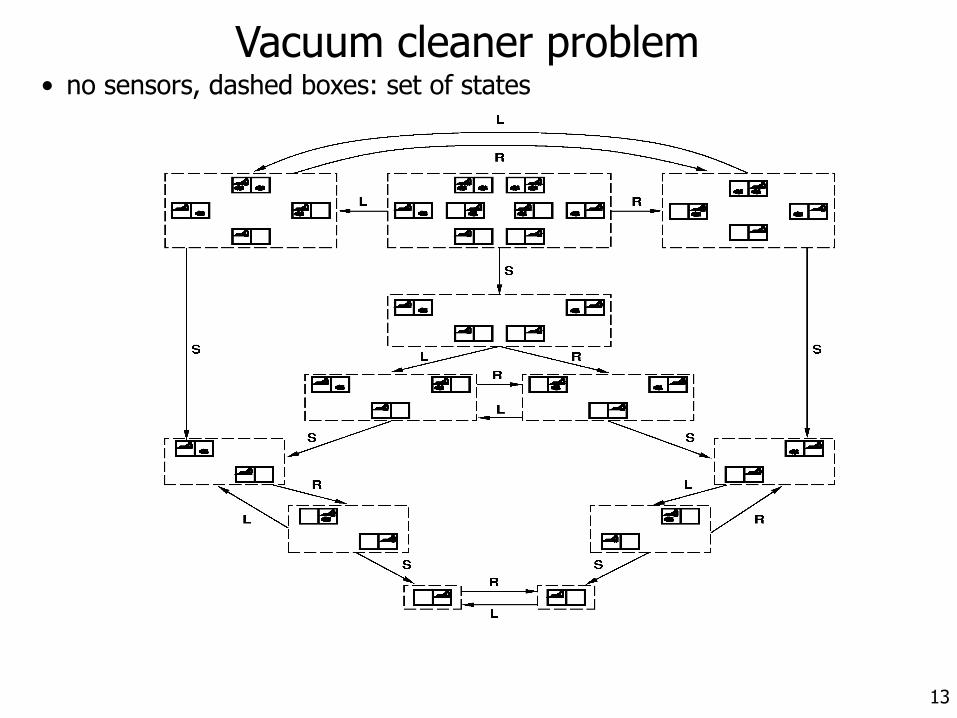
• no sensors, dashed boxes: set of statesVacuum cleaner problem

14

Examples (real world)

• Finding routes – Routing in networks – Automatic travel routes – Airline planning systems

• Traveling Salesman Problem (TSP)

• VLSI Layout – Chip layout

• Robot navigation – Generalization of route-finding problem (continuous space)

• Search in the Internet

15

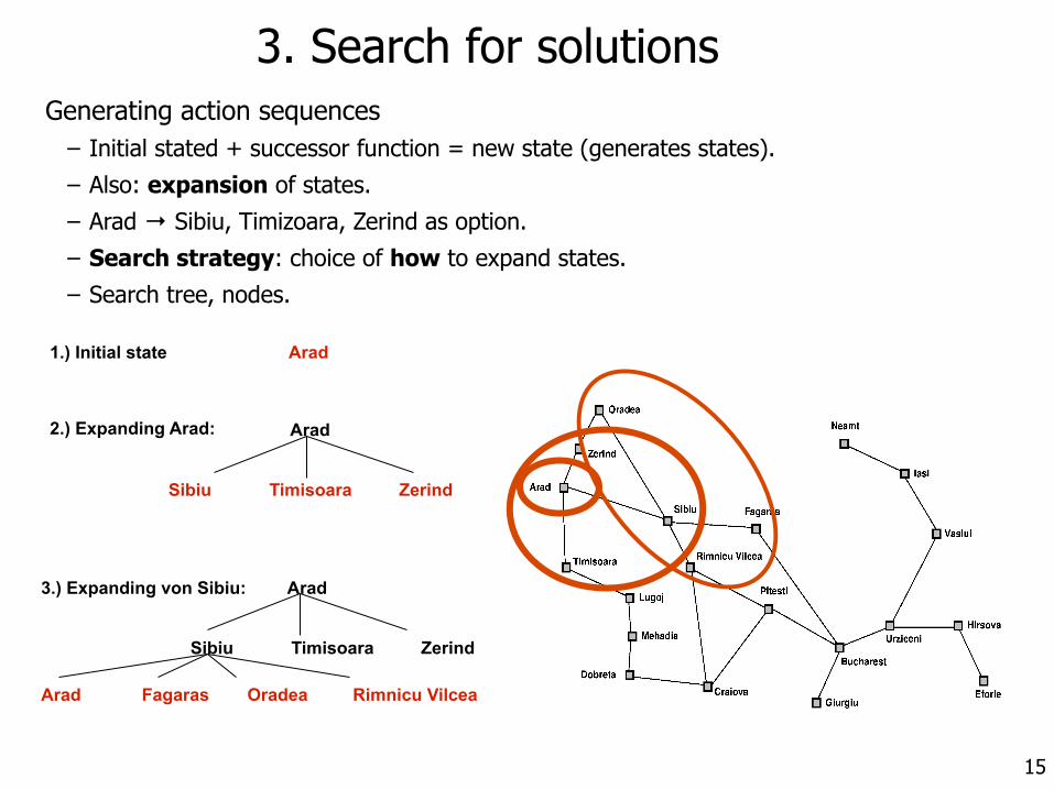
3. Search for solutionsGenerating action sequences

– Initial stated + successor function = new state (generates states). – Also: expansion of states. – Arad → Sibiu, Timizoara, Zerind as option. – Search strategy: choice of how to expand states. – Search tree, nodes.

Arad1.) Initial state

2.) Expanding Arad: Arad

Sibiu Timisoara Zerind

Sibiu Timisoara Zerind

3.) Expanding von Sibiu: Arad

Arad Fagaras Oradea Rimnicu Vilcea

16

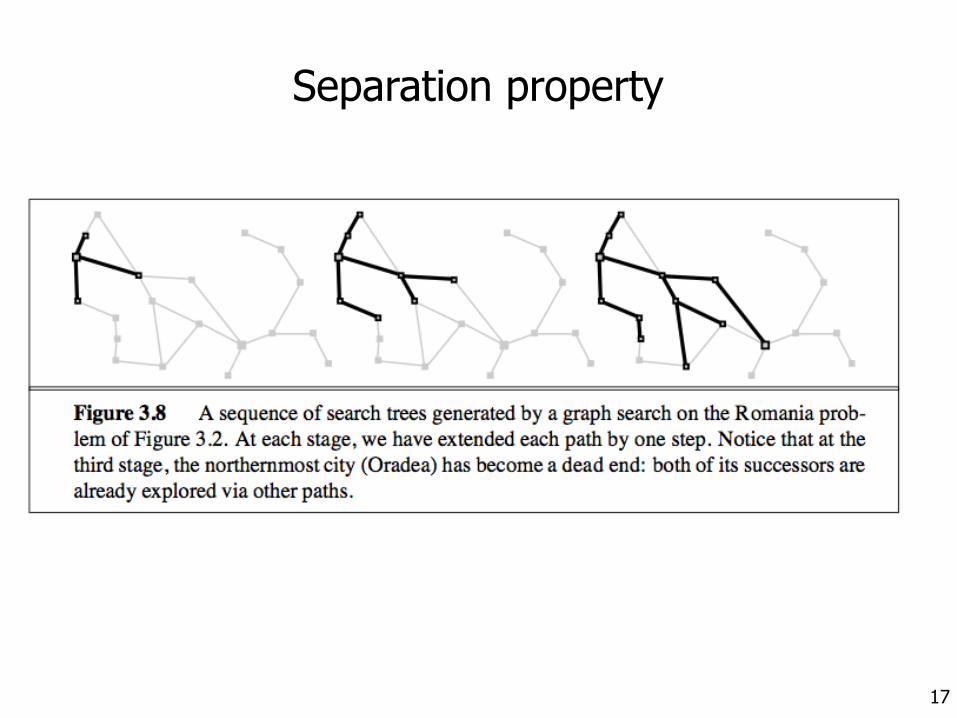
Separation property

17

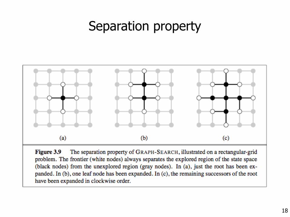
Separation property

18

19

Infrastructure for search algorithms

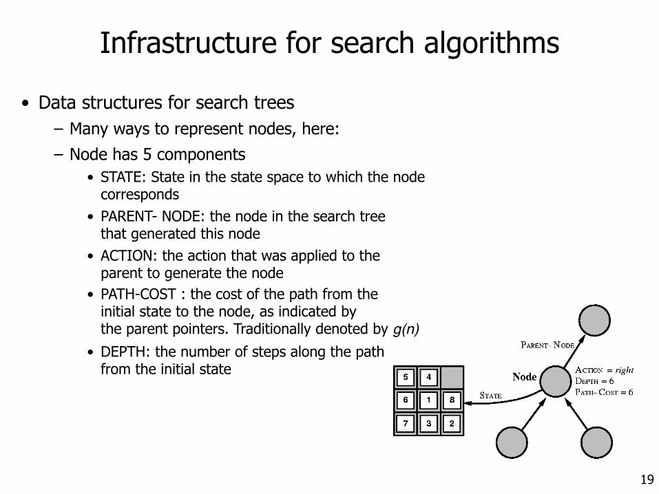
• Data structures for search trees – Many ways to represent nodes, here: – Node has 5 components

• STATE: State in the state space to which the node corresponds

• PARENT- NODE: the node in the search tree that generated this node

• ACTION: the action that was applied to the parent to generate the node

• PATH-COST : the cost of the path from the initial state to the node, as indicated by the parent pointers. Traditionally denoted by g(n)

• DEPTH: the number of steps along the path from the initial state

20

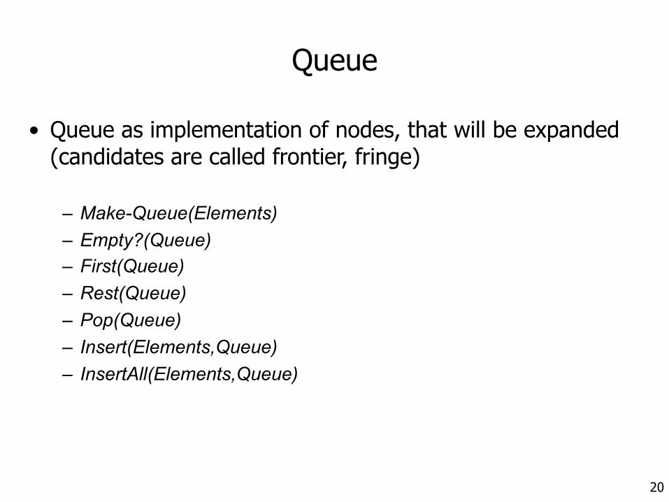
Queue

• Queue as implementation of nodes, that will be expanded (candidates are called frontier, fringe)

– Make-Queue(Elements) – Empty?(Queue) – First(Queue) – Rest(Queue) – Pop(Queue) – Insert(Elements,Queue) – InsertAll(Elements,Queue)

21

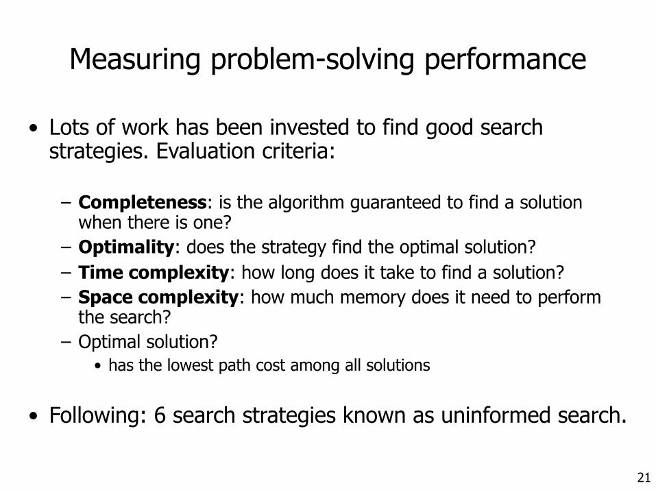
Measuring problem-solving performance

• Lots of work has been invested to find good search strategies. Evaluation criteria:

– Completeness: is the algorithm guaranteed to find a solution when there is one?

– Optimality: does the strategy find the optimal solution? – Time complexity: how long does it take to find a solution? – Space complexity: how much memory does it need to perform

the search? – Optimal solution?

• has the lowest path cost among all solutions

• Following: 6 search strategies known as uninformed search.

22

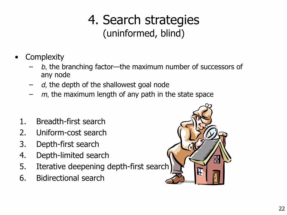
4. Search strategies (uninformed, blind)

1. Breadth-first search 2. Uniform-cost search 3. Depth-first search 4. Depth-limited search 5. Iterative deepening depth-first search 6. Bidirectional search

• Complexity – b, the branching factor—the maximum number of successors of

any node – d, the depth of the shallowest goal node – m, the maximum length of any path in the state space

23

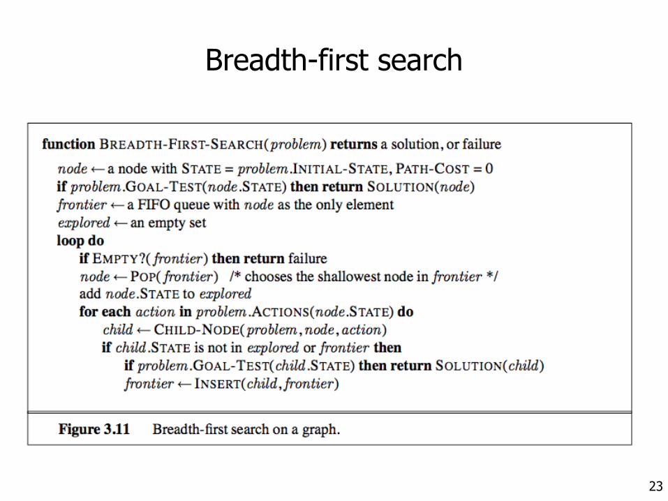
Breadth-first search

24

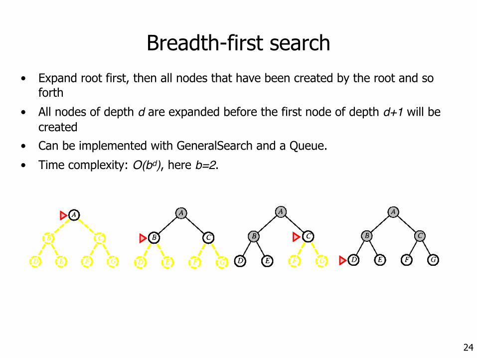
Breadth-first search• Expand root first, then all nodes that have been created by the root and so

forth

• All nodes of depth d are expanded before the first node of depth d+1 will be created

• Can be implemented with GeneralSearch and a Queue.

• Time complexity: O(bd), here b=2.

25

Breadth-first search (2)

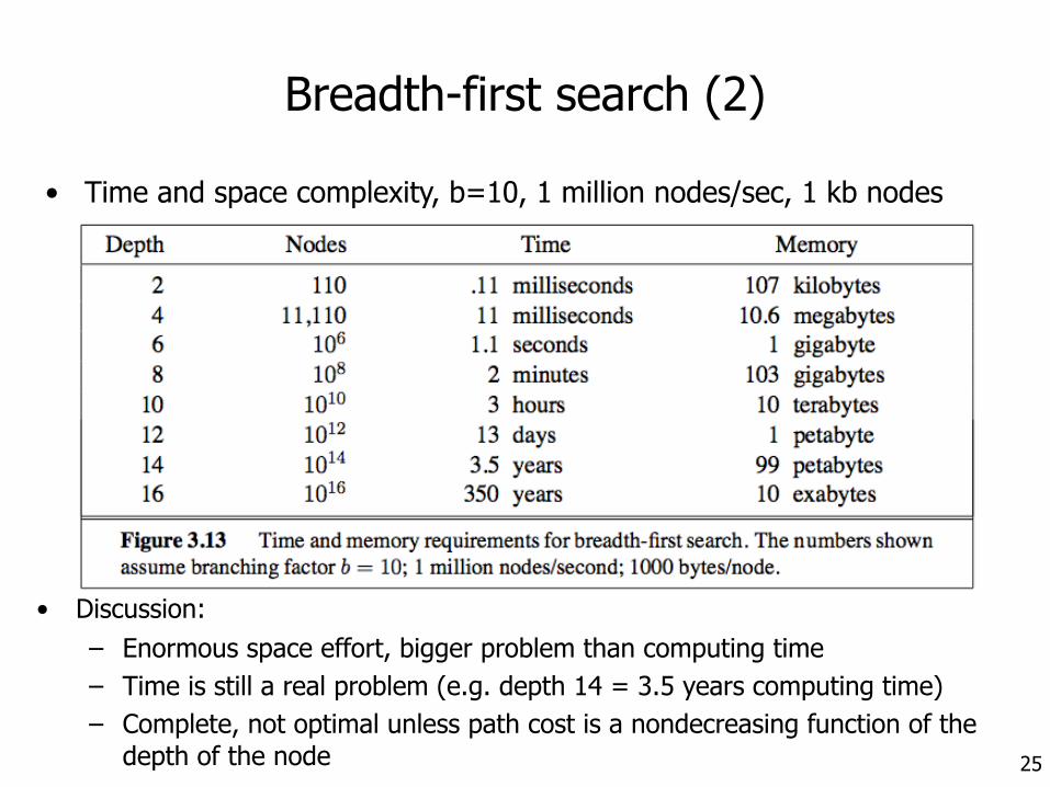
• Time and space complexity, b=10, 1 million nodes/sec, 1 kb nodes

• Discussion: – Enormous space effort, bigger problem than computing time – Time is still a real problem (e.g. depth 14 = 3.5 years computing time) – Complete, not optimal unless path cost is a nondecreasing function of the

depth of the node

26

Uniform-cost search

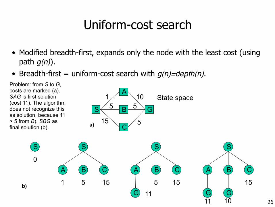
• Modified breadth-first, expands only the node with the least cost (using path g(n)).

• Breadth-first = uniform-cost search with g(n)=depth(n).Problem: from S to G, costs are marked (a). SAG is first solution (cost 11). The algorithm does not recognize this as solution, because 11 > 5 from B). SBG as final solution (b).

A

B

C

S G

15 5

515

10 State space

a)

S

0

S

BA C

1 5 15b)

S

BA C

G 11

5 15

S

BA C

G11

15G

10

27

Uniform-cost search (2)

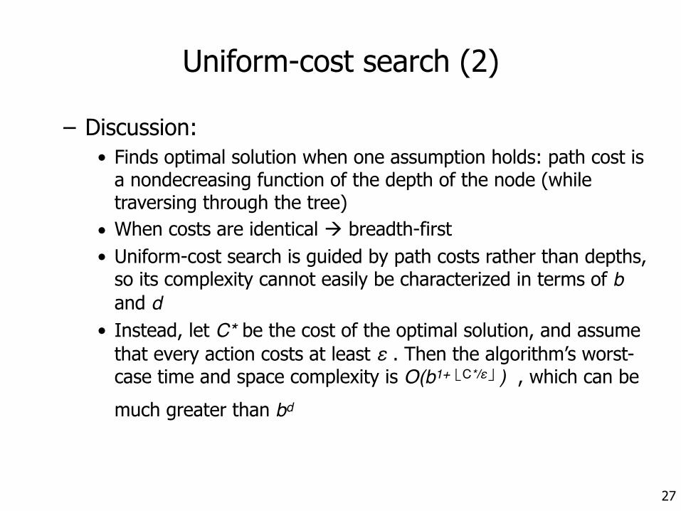
– Discussion: • Finds optimal solution when one assumption holds: path cost is

a nondecreasing function of the depth of the node (while traversing through the tree)

• When costs are identical ! breadth-first • Uniform-cost search is guided by path costs rather than depths,

so its complexity cannot easily be characterized in terms of b and d

• Instead, let C* be the cost of the optimal solution, and assume that every action costs at least ε . Then the algorithm’s worst-case time and space complexity is O(b1+⎣C*/ε⎦) , which can be

much greater than bd

28

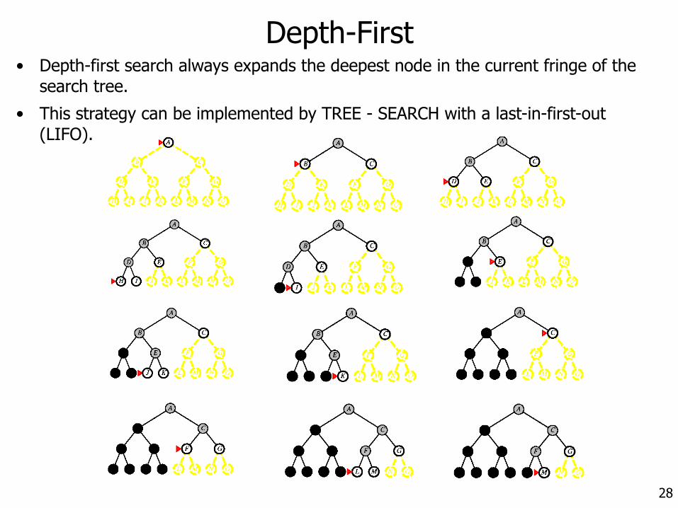
Depth-First• Depth-first search always expands the deepest node in the current fringe of the

search tree.

• This strategy can be implemented by TREE - SEARCH with a last-in-first-out (LIFO).

29

Depth-First (2)

• Discussion: – Moderate space complexity (only single path in memory), max.

depth m and branching factor b = O(bm) nodes. – Comparison to breadth-first: 156 KB instead of 10 EB with depth

16, a factor of 1:7 trillion times less memory. – Time: O(bm). – Better as breath-first for problems with lots of solutions – But: you can get stuck if wrong choice leads to very long path (or

even infinite) – → Depth-first not complete and not optimal. – Thus: avoid using depth-first with large or infinite maximal depths

30

Depth-First (3)

• Backtracking: – A variant of depth-first search called backtracking search uses still

less memory. – Only one successor is generated at a time rather than all

successors; each partially expanded node remembers which successor to generate next.

– In this way, only O(m) memory is needed rather than O(bm)– Backtracking search facilitates yet another memory-saving (and

time-saving) trick: the idea of generating a successor by modifying the current state description directly rather than copying it first. This reduces the memory requirements to just one state description and O(m) actions.

– For this to work, we must be able to undo each modification when we go back to generate the next successor. For problems with large state descriptions, such as robotic assembly, these techniques are critical to success.

31

Depth-limited search

• Avoids disadvantage of depth-first through cut off max. depth of path • Can be implemented with special algorithm or with GeneralSearch that

includes operators, which save current. • Example: Search for solution of a path having 20 cities. We know that

max. depth=19 – New operator: Suppose you are in city A and you have done < 19 steps.

We then generate a new state in city B with path length that is increased by one.

• We find the solution guaranteed (if there is one) but algorithm is not optimal. • Time and space complexity resembles depth-first search

• ! Depth-limited search is complete but not optimal

32

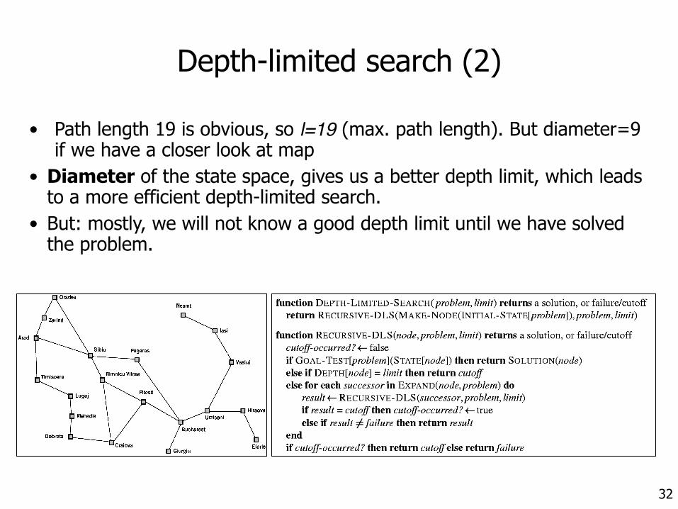
Depth-limited search (2)

• Path length 19 is obvious, so l=19 (max. path length). But diameter=9 if we have a closer look at map

• Diameter of the state space, gives us a better depth limit, which leads to a more efficient depth-limited search.

• But: mostly, we will not know a good depth limit until we have solved the problem.

33

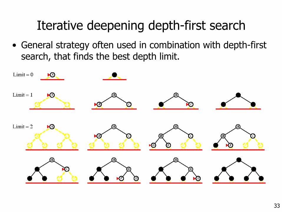
Iterative deepening depth-first search• General strategy often used in combination with depth-first

search, that finds the best depth limit.

34

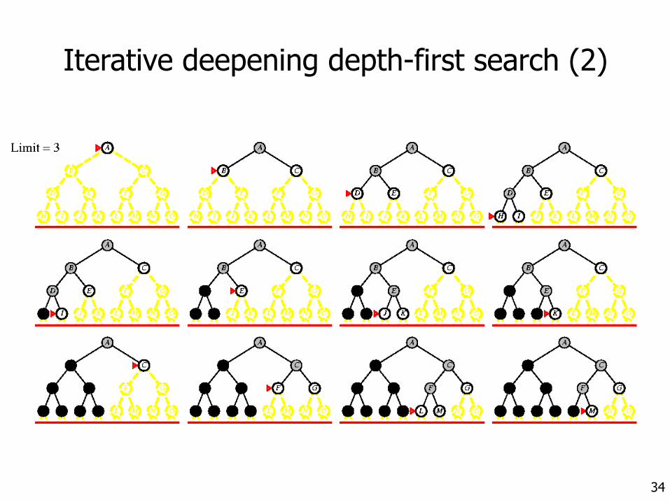
Iterative deepening depth-first search (2)

35

Iterative deepening depth-first search (3)

• Discussion: – Combination of advantages of breadth-first and depth-first search. – Iterative deepening depth-first search is complete and optimal1. – States as in depth-first, approx. 11% more nodes. – Time: O(bd) – Space: O(bd) – In general: iterative deepening if state space is large and depth of

solution is unknown

1: Complete, when the branching factor is finite and optimal when the path cost is a nondecreasing function of the depth of the node

36

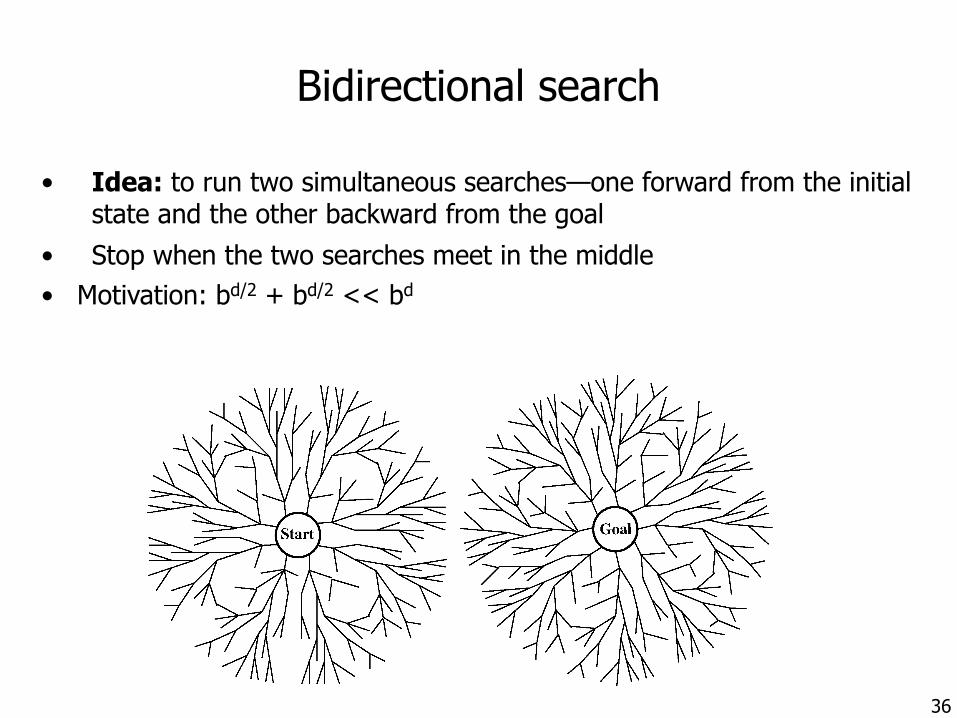
Bidirectional search

• Idea: to run two simultaneous searches—one forward from the initial state and the other backward from the goal

• Stop when the two searches meet in the middle • Motivation: bd/2 + bd/2 << bd

37

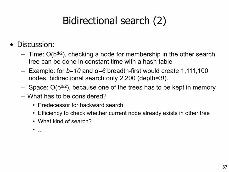
Bidirectional search (2)

• Discussion: – Time: O(bd/2), checking a node for membership in the other search

tree can be done in constant time with a hash table – Example: for b=10 and d=6 breadth-first would create 1,111,100

nodes, bidirectional search only 2,200 (depth=3!). – Space: O(bd/2), because one of the trees has to be kept in memory – What has to be considered?

• Predecessor for backward search • Efficiency to check whether current node already exists in other tree • What kind of search? • ...

38

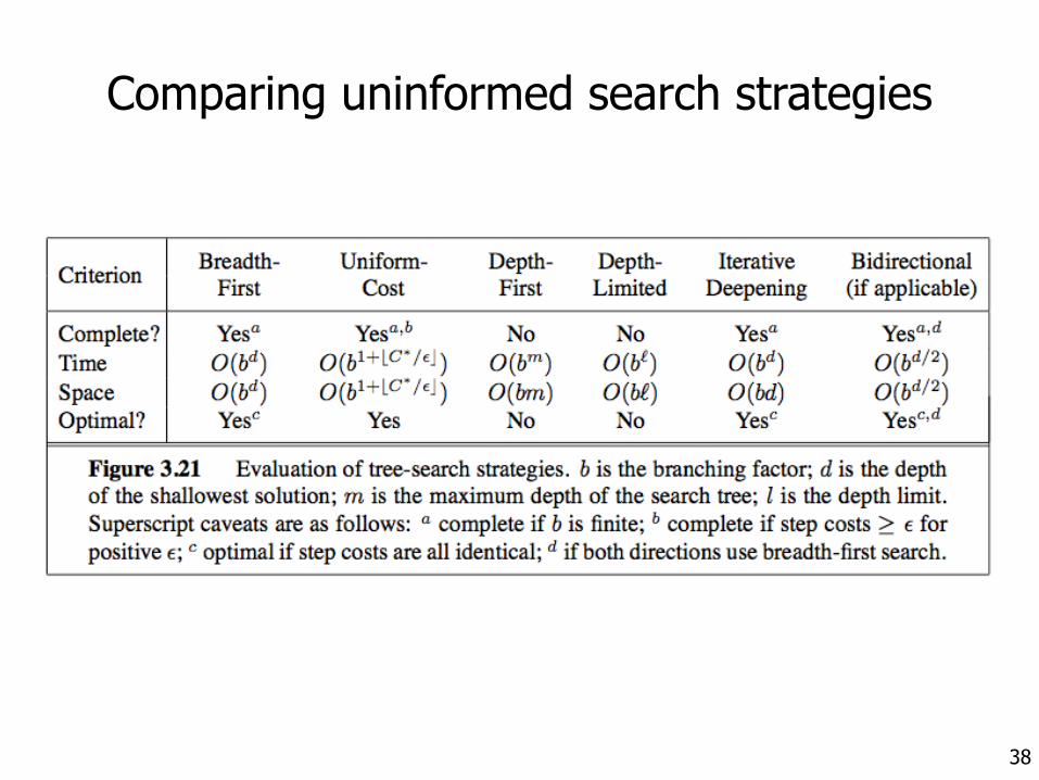
Comparing uninformed search strategies

39

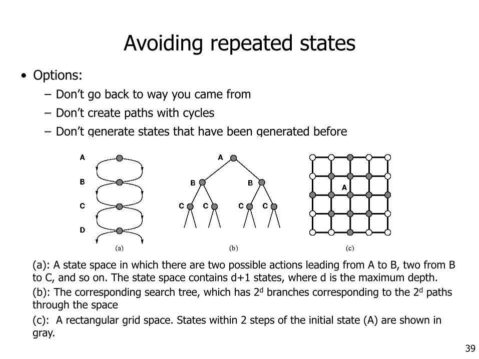
Avoiding repeated states• Options:

– Don’t go back to way you came from – Don’t create paths with cycles – Don’t generate states that have been generated before

(a): A state space in which there are two possible actions leading from A to B, two from B to C, and so on. The state space contains d+1 states, where d is the maximum depth. (b): The corresponding search tree, which has 2d branches corresponding to the 2d paths through the space (c): A rectangular grid space. States within 2 steps of the initial state (A) are shown in gray.

40

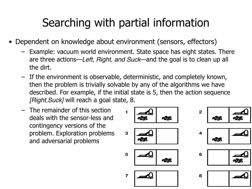
Searching with partial information• Dependent on knowledge about environment (sensors, effectors)

– Example: vacuum world environment. State space has eight states. There are three actions—Left, Right, and Suck—and the goal is to clean up all the dirt.

– If the environment is observable, deterministic, and completely known, then the problem is trivially solvable by any of the algorithms we have described. For example, if the initial state is 5, then the action sequence [Right,Suck] will reach a goal state, 8.

– The remainder of this section deals with the sensor-less and contingency versions of the problem. Exploration problems and adversarial problems

41

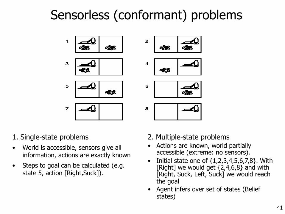
1. Single-state problems • World is accessible, sensors give all

information, actions are exactly known

• Steps to goal can be calculated (e.g. state 5, action [Right,Suck]).

2. Multiple-state problems • Actions are known, world partially

accessible (extreme: no sensors). • Initial state one of {1,2,3,4,5,6,7,8}. With

[Right] we would get {2,4,6,8} and with [Right, Suck, Left, Suck] we would reach the goal

• Agent infers over set of states (Belief states)

Sensorless (conformant) problems

42

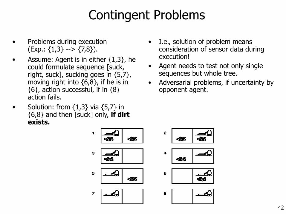
• Problems during execution (Exp.: {1,3} --> {7,8}).

• Assume: Agent is in either {1,3}, he could formulate sequence [suck, right, suck], sucking goes in {5,7}, moving right into {6,8}, if he is in {6}, action successful, if in {8} action fails.

• Solution: from {1,3} via {5,7} in {6,8} and then [suck] only, if dirt exists.

• I.e., solution of problem means consideration of sensor data during execution!

• Agent needs to test not only single sequences but whole tree.

• Adversarial problems, if uncertainty by opponent agent.

Contingent Problems

43

• Assumption: Agent has no information about effect of his actions (most difficult situation).

• Agent needs to experiment, this is a kind of search, but search in real world not in model world.

• If agent “survives”, learns his world like through a map that he can use later.

• Single-state and multiple-state problems are solvable with similar search techniques, contingency problems need more complex techniques.

Exploration problems

44

Summary

• Before an agent can start searching for solutions, it must formulate a goal and then use the goal to formulate a problem.

• A problem consists of four parts: the initial state, a set of actions, a goal test function, and a path cost function. The environment of the problem is represented by a state space. A path through the state space from the initial state to a goal state is a solution.

• In real life, most problems are ill-defined; but with some analysis, many problems can fit into the state space model.

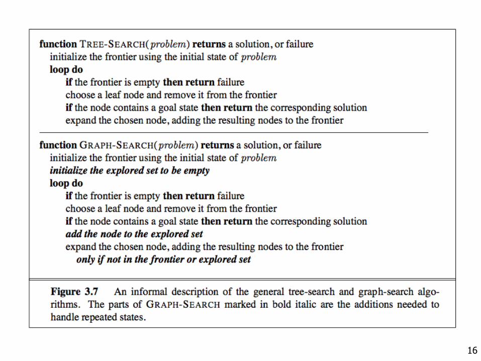
• A single, general TREE- SEARCH algorithm can be used to solve any problem; specific variants of the algorithm embody different strategies.

• Search algorithms are judged on the basis of completeness, optimality, time complexity, and space complexity. Complexity depends on b, the branching factor in the state space, and d, the depth of the shallowest solution.

45

Summary (2)

• Breadth-first search selects the shallowest unexpanded node in the search tree for expansion. It is complete, optimal for unit step costs, and has time and space complexity of O(bd). The space complexity makes it impractical in most cases. Uniform-cost search is similar to breadth-first search but expands the node with lowest path cost, g(n). It is complete and optimal provided step costs exceed some positive bound ε.

• Depth-first search selects the deepest unexpanded node in the search tree for expansion. It is neither complete nor optimal, and has time complexity of O(bm) and space complexity of O(bm), where m is the maximum depth of any path in the state space.

• Depth-limited search imposes a fixed depth limit on a depth-first search.

46

Summary (3)

• Iterative deepening search calls depth-limited search with increasing limits until a goal is found. It is complete, optimal for unit step costs, and has time complexity of O(bd) and space complexity of O(bd).

• Bidirectional search can enormously reduce time complexity, but is not always applicable and may be impractical because of its space complexity.

• When the environment is partially observable, the agent can apply search algorithms in the space of belief states, or sets of possible states that the agent might be in. In some cases, a single solution sequence can be constructed; in other cases, a contingency plan is required.