Embed Size (px)
Citation preview

SOLVING LINEAR SYSTEMS
Linear systems Ax = b occur widely in applied math-
ematics. They occur as direct formulations of “real
world” problems; but more often, they occur as a part
of the numerical analysis of some other problem. As
examples of the latter, we have the numerical solution
of systems of nonlinear equations, ordinary and par-
tial differential equations, integral equations, and the
solution of optimization problems.
There are many ways of classifying linear systems.
Size: Small, moderate and large. This of course varies
with the machine you are using. Most PCs are now
being sold with a memory of 64 to 128 megabytes
(MB), my own HP workstation has 768 MB, and the
Weeg computer center’s SGI shared memory parallel
computer has a memory of 2 gigabytes (GB).

For a matrix A of order n × n, it will take 8n2 bytes
to store it in double precision. Thus a matrix of order
4000 will need around 128 MB of storage. The latter
would be too large for most present day PCs, if the
matrix was to be stored in the computer’s memory.
Sparse vs. Dense. Many linear systems have a matrix
A in which almost all the elements are zero. These
matrices are said to be sparse. For example, it is quite
common to work with tridiagonal matrices
A =
a1 c1 0 · · · 0b2 a2 c2 0 ...0 b3 a3 c3... . . .0 · · · bn an
in which the order is 104 or much more. For such
matrices, it does not make sense to store the zero ele-
ments; and the sparsity should be taken into account
when solving the linear system Ax = b. Also, the
sparsity need not be as regular as in this example.

Special properties: Often the matrix will have some
other special properties. For example, A might be
symmetric, tridiagonal, banded,
ai,j = 0 for |i − j| > p
or positive definite,
(Ax, x) > 0 for all x ∈ Cn, x �= 0
All of these properties can be used to develop more
efficient and accurate methods for solving Ax = b.

METHODS OF SOLUTION
There are two general categories of numerical methods
for solving Ax = b.
Direct Methods: These are methods with a finite num-
ber of steps; and they end with the exact solution x,
provided that all arithmetic operations are exact. The
most used of these methods is Gaussian elimination,
which we will begin with. There are other direct meth-
ods, and we will study them later in connection with
solving the matrix eigenvalue problem.
Iteration Methods: These are used in solving all types
of linear systems, but they are most commonly used
with large sparse systems, especially those produced
by discretizing partial differential equations. This is
an extremely active area of research.

SOLVING LINEAR SYSTEMS
We want to solve the linear system Ax = b:
a1,1 · · · a1,n... . . . ...
an,1 · · · an,n
x1...
xn
=
b1...
bn
This will be done by the method used in beginning
algebra, by successively eliminating unknowns from
equations, until eventually we have only one equation
in one unknown. This process is known as Gaussian
elimination. To help us keep track of the steps of this
process, we will denote the initial system by
A(1)x = b(1):
a(1)1,1 · · · a
(1)1,n
... . . . ...
a(1)n,1 · · · a
(1)n,n
x1...
xn
=
b(1)1...
b(1)n
Initially we will make the assumption that every pivot
element will be nonzero; and later we remove this
assumption.

Step 1. We will eliminate x1 from equations 2 thru
n. Begin by defining the multipliers
mi,1 =a(1)i,1
a(1)1,1
, i = 2, ..., n
Here we are assuming the pivot element a(1)1,1 �= 0.
Then in succession, multiply mi,1 times row 1 (called
the pivot row) and subtract the result from row i.
This yields new matrix elements
a(2)i,j = a
(1)i,j − mi,1a
(1)1,j , j = 2, ..., n
b(2)i = b
(1)i − mi,1b
(1)1
for i = 2, ..., n.
Note that the index j does not include j = 1. The
reason is that with the definition of the multiplier mi,1,
it is automatic that
a(2)i,1 = a
(1)i,1 − mi,1a
(1)1,1 = 0, i = 2, ..., n

The linear system is now denoted by A(2)x = b(2):
a(1)1,1 a
(1)1,2 · · · a
(1)1,n
0 a(2)2,2 a
(2)2,n
... ... . . . ...
0 a(2)n,2 · · · a
(2)n,n
x1x2...
xn
=
b(1)1
b(2)2...
b(2)n
Step k: Assume that for i = 1, ..., k − 1 the unknown
xi has been eliminated from equations i + 1 thru n.
We have the system A(k)x = b(k)
a(1)1,1 a
(1)1,2 · · · a
(1)1,n
0 a(2)2,2 · · · a
(2)2,n
. . . . . . ...... 0 a
(k)k,k · · · a
(k)k,n
... ... . . . ...
0 · · · 0 a(k)n,k · · · a
(k)n,n
x1x2
...
xn
=
b(1)1
b(2)2...
b(k)k...
b(k)n
We want to eliminate unknown xk from equations
k + 1 thru n.

Begin by defining the multipliers
mi,k =a(k)i,k
a(k)k,k
, i = k + 1, ..., n
The pivot element is a(k)k,k, and we assume it is nonzero.
Using these, we eliminate xk from equations k + 1
thru n. Multiply mi,k times row k (the pivot row)
and subtract from row i, for i = k + 1 thru n.
a(k+1)i,j = a
(k)i,j − mi,ka
(k)k,j , j = k + 1, ..., n
b(k+1)i = b
(k)i − mi,kb
(k)k
for i = k + 1, ..., n. This yields the linear system
A(k)x = b(k):

a(1)1,1 · · · a
(1)1,n
0 . . . ...
a(k)k,k a
(k)k,k+1 · · · a
(k)k,n
... 0 a(k+1)k+1,k+1 a
(k+1)k+1,n
... ... . . . ...
0 · · · 0 a(k+1)n,k+1 · · · a
(k+1)n,n
x1...
xkxk+1
...xn
=
b(1)1...
b(k)k
b(k+1)k+1
...
b(k+1)n
Doing this for k = 1, 2, ..., n leads to an upper trian-
gular system of linear equations A(n)x = b(n):
a(1)1,1 · · · a
(1)1,n
0 . . . ...... . . .
0 · · · 0 a(n)n,n
x1......
xn
=
b(1)1......
b(n)n

At each step, we have assumed for the pivot element
that
a(k)k,k �= 0
Later we remove this assumption. For now, we con-
sider the solution of the upper triangular system
A(n)x = b(n).
To avoid the superscripts, and to emphasize we are
now solving an upper triangular system, denote this
system by
Ux = g
u1,1 · · · u1,n0 . . . ...... . . .0 · · · 0 un,n
x1......
xn
=
g1......
gn
This is the linear system
u1,1x1 + u1,2x2 + · · · + u1,n−1xn−1 + u1,nxn = g1...
un−1,n−1xn−1 + un−1,nxn = gn−1un,nxn = gn

u1,1x1 + u1,2x2 + · · · + u1,n−1xn−1 + u1,nxn = g1...
un−1,n−1xn−1 + un−1,nxn = gn−1un,nxn = gn
We solve for xn, then xn−1, and backwards to x1.
This process is called back substitution.
xn =gn
un,n
uk =gk −
{uk,k+1xk+1 + · · · + uk,nxn
}
uk,k
for k = n − 1, ..., 1.
Examples of the process of producing A(n)x = b(n)
and of solving Ux = g are given in the text. They
are simply a more carefully defined and methodical
version of what you have done in high school algebra.

QUESTIONS
• How do we remove the assumption on the pivot
elements?
• How many operations are involved in this proce-
dure?
• How much error is there in the computed solution
due to rounding errors in the calculations?
• Later (if there is time), how does the machine
architecture affect the implementation of this al-
gorithm.
Before doing this, we consider a result on factoring
matrices that is associated with Gaussian elimination.

THE LU FACTORIZATION
Using the multipliers from Gaussian elimination, de-
fine the lower triangular matrix
L =
1 0 0 · · · 0m2,1 1 0m3,1 m3,2 1 ...
... . . .mn,1 mn,2 · · · mn,n−1 1
Recall the upper triangular matrix U = A(n). Then
A = LU
This is called the LU-factorization of the matrix A.

Proof. The proof is obtained by looking at the (i, j)
element of LU ,
(LU)i,j =[mi,1, ..., mi,i−1, 1, 0, ..., 0
]
u1,j...
uj,j0...0
We consider separately the cases of i ≤ j and i > j.
With the first case, we have more nonzero elements
in the column U∗,j than in the row Li,∗. Thus
(LU)i,j = mi,1u1,j + · · · + mi,i−1ui−1,j + ui,j
The elements ui,j are given by
ui,j = a(i)i,j , j = i, ..., n, i = 1, ..., n

Recall that
a(2)i,j = a
(1)i,j − mi,1a
(1)1,j , j = 2, ..., n
for i = 2, ..., n. Then
mi,1u1,j = mi,1a(1)1,j = a
(1)i,j − a
(2)i,j
Similarly,
mi,2u2,j = mi,2a(2)2,j = a
(2)i,j − a
(3)i,j
...
mi,i−1ui−1,j = mi,i−1a(i−1)i−1,j = a
(i−1)i,j − a
(i)i,j
Combining these results,
(LU)i,j = mi,1u1,j + · · · + mi,i−1ui−1,j + ui,j
=(a(1)i,j − a
(2)i,j
)+
(a(2)i,j − a
(3)i,j
)
+ · · · +(a(i−1)i,j − a
(i)i,j
)+ a
(i)i,j
= a(1)i,j = ai,j
The second case, in which i > j, is given in the text.

EXAMPLE
In the text, we consider the linear system
1 2 12 2 3
−1 −3 0
x1x2x3
=
032
Gaussian elimination leads to
1 2 10 −2 1
0 0 12
x1x2x3
=
0312
with multipliers
m2,1 = 2, m3,1 = −1, m3,2 =1
2
Then
1 0 02 1 0
−1 12 1
1 2 10 −2 1
0 0 12
=
1 2 12 2 3
−1 −3 0

In Matlab, you can find the LU factorization of a ma-
trix using the function lu. For example,
[L U P ] = lu(A)
yields a lower triangular matrix L, an upper triangular
matrix U , and a permuation matrix P , for which
LU = PA
The reason for this arises in a modification of Gaus-
sian elimination, one which eliminates our assumption
regarding the pivot elements being nonzero and simul-
taneously improves the error behaviour of Gaussian
elimination.

AN OPERATIONS COUNT
How many operations are expended in solving Ax =
b using Gaussian elimination? To calculate this, we
must return to the formal definitions, of both A(k)x =
b(k) and the solution of Ux = g.
Step 1. Multipliers: n − 1 divisions.
A(1) → A(2): (n − 1)2 additions and multiplications.
[Note that we consider additions and subtractions as
the same type of operation.]
b(1) → b(2): n − 1 additions and multiplications.
Step 2. Multipliers: n − 2 divisions.
A(2) → A(3): (n − 2)2 additions and multiplications.
b(2) → b(3): n − 2 additions and multiplications.

Step n − 1. Multipliers: 1 division.
A(n) → A(n−1): 1 addition and multiplication.
b(n−1) → b(n): 1 addition and multiplication.
Thus we have the following totals for the transforma-
tion of A to U = A(n).
Divisions. (n − 1) + (n − 2) + · · · + 1
Additions. (n − 1)2 + (n − 2)2 + · · · + 1
Multiplications. (n − 1)2 + (n − 2)2 + · · · + 1
To add these up, we need the following general for-
mulas.
p∑j=1
j =p(p + 1)
2
p∑j=1
j2 =p(p + 1)(2p + 1)
6
These can proven using mathematical induction.
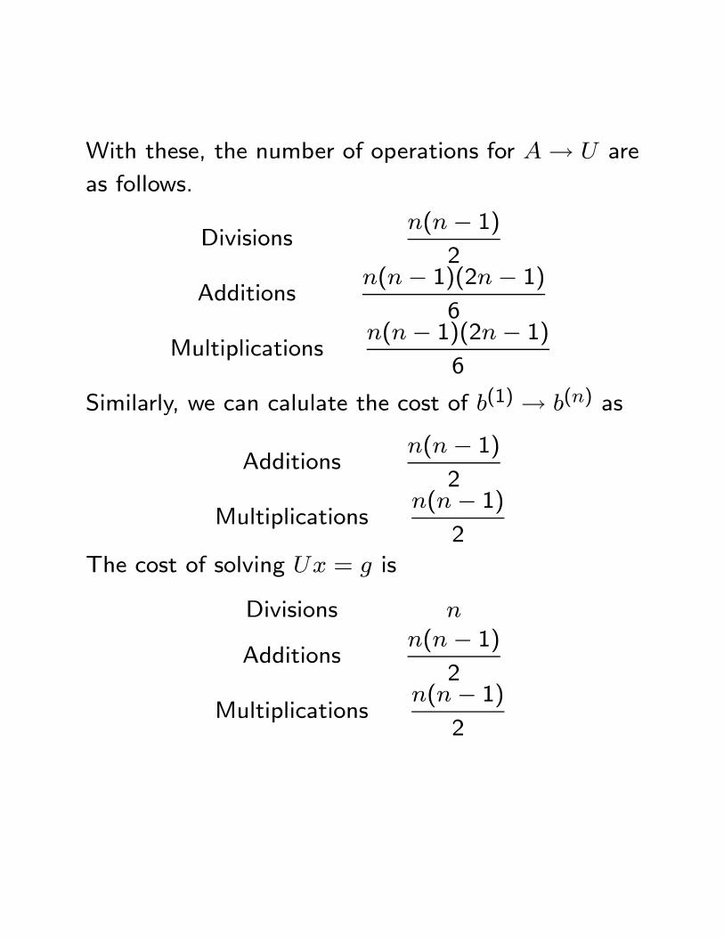
With these, the number of operations for A → U are
as follows.
Divisionsn(n − 1)
2
Additionsn(n − 1)(2n − 1)
6
Multiplicationsn(n − 1)(2n − 1)
6
Similarly, we can calulate the cost of b(1) → b(n) as
Additionsn(n − 1)
2
Multiplicationsn(n − 1)
2
The cost of solving Ux = g is
Divisions n
Additionsn(n − 1)
2
Multiplicationsn(n − 1)
2

On some machines, the cost of a division is much more
than that of a multiplication; whereas on others there
is not any important difference.
For this last case, we usually combine the additions
and subtractions to obtain the following costs.
MD(A → U) =n
(n2 − 1
)
3
MD(b(1) → g) =n(n − 1)
2
MD(Find x) =n(n + 1)
2
For additions and subtractions, we have
AS(A → U) =n(n − 1)(2n − 1)
6
AS(b(1) → g) =n(n − 1)
2
AS(Find x) =n(n − 1)
2
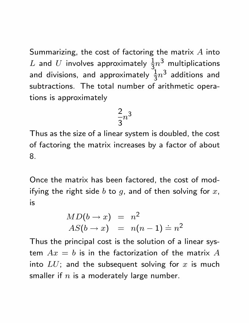
Summarizing, the cost of factoring the matrix A into
L and U involves approximately 13n3 multiplications
and divisions, and approximately 13n3 additions and
subtractions. The total number of arithmetic opera-
tions is approximately
2
3n3
Thus as the size of a linear system is doubled, the cost
of factoring the matrix increases by a factor of about
8.
Once the matrix has been factored, the cost of mod-
ifying the right side b to g, and of then solving for x,
is
MD(b → x) = n2
AS(b → x) = n(n − 1).= n2
Thus the principal cost is the solution of a linear sys-
tem Ax = b is in the factorization of the matrix A
into LU ; and the subsequent solving for x is much
smaller if n is a moderately large number.

We often wish to solve linear systems Ax = b with
varying vectors b, and A unchanged. For such cases,
it is important to keep the information used in pro-
ducing L and U , as this this is the costly portion of
the solution process.
In the machine, store the elements ui,j and mi,j into
the portions of A with the same subscripts. This
can be done, as those positions are no longer being
changed; and for the portion below the diagonal, those
elements are being set to zero in A.
To solve m systems
Ax(�) = b(�), � = 1, ..., m
for m different right hand vectors b(�), the operations
cost will be
MD =n
(n2 − 1
)
3+ mn2 .
= 13n3 + mn2
AS =n(n − 1)(2n − 1)
2+ mn(n − 1)
.= 1
3n3 + mn2

CALCULATING AN INVERSE
To find the inverse of a matrix A amounts to solving
the equation
AX = I
In partioned form,
A[X∗,1, ..., X∗,n] =[e(1), ..., e(n)
]
which yields the n equivalent linear systems
AX∗,k = e(k), k = 1, ..., n
Thus the cost of calculating the inverse X = A−1 is
approximately
2
3n3 + 2n3 =
8
3n3
This is only around 4 times the cost of solving a single
system Ax = b.