Embed Size (px)
Citation preview
15 September 2003
INFORMS Practice 2002 1
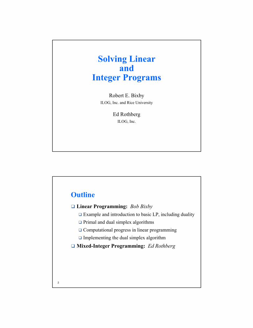
Solving Linear and
Integer Programs
Robert E. BixbyILOG, Inc. and Rice University
Ed RothbergILOG, Inc.
2
OutlineLinear Programming: Bob Bixby
Example and introduction to basic LP, including dualityPrimal and dual simplex algorithmsComputational progress in linear programmingImplementing the dual simplex algorithm
Mixed-Integer Programming: Ed Rothberg
15 September 2003
INFORMS Practice 2002 2
3
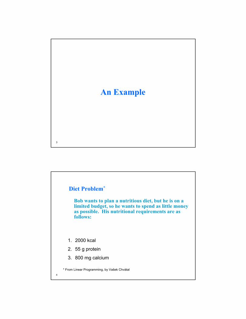
An Example
4
Diet Problem*
Bob wants to plan a nutritious diet, but he is on a limited budget, so he wants to spend as little money as possible. His nutritional requirements are as follows:
1. 2000 kcal
2. 55 g protein
3. 800 mg calcium
* From Linear Programming, by Vaŝek Chvátal
15 September 2003
INFORMS Practice 2002 3
5
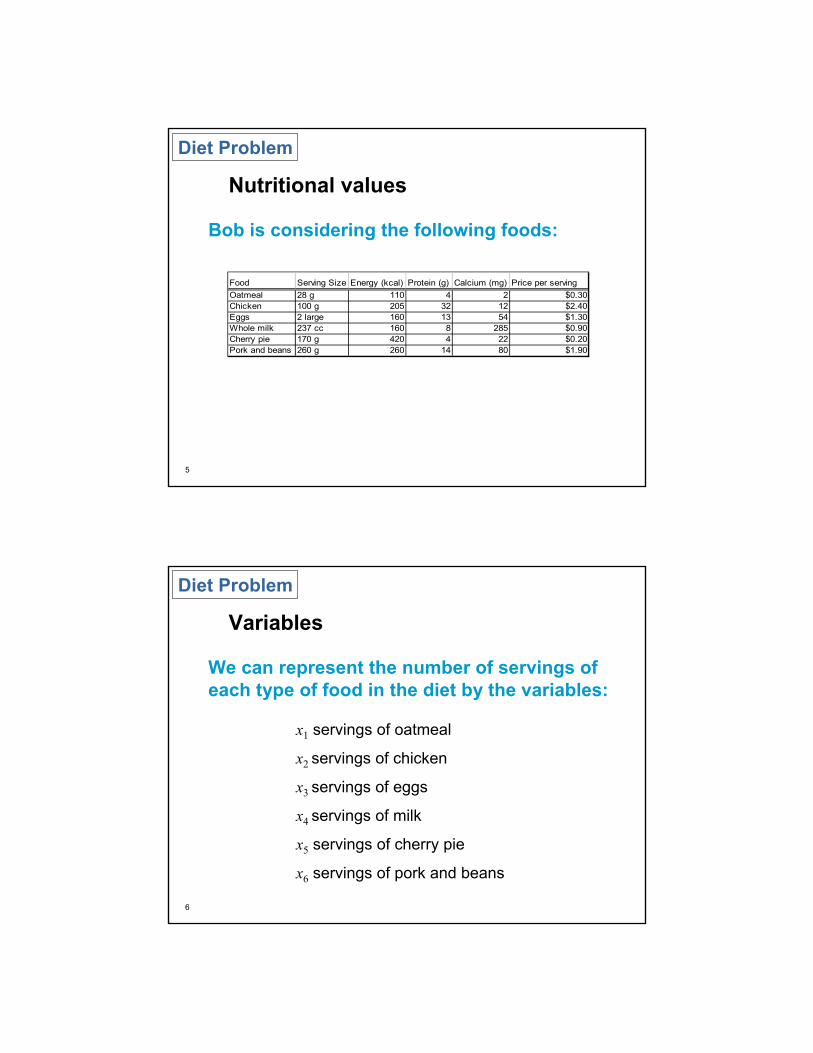
Nutritional values
Diet Problem
Bob is considering the following foods:
Food Serving Size Energy (kcal) Protein (g) Calcium (mg) Price per servingOatmeal 28 g 110 4 2 $0.30Chicken 100 g 205 32 12 $2.40Eggs 2 large 160 13 54 $1.30Whole milk 237 cc 160 8 285 $0.90Cherry pie 170 g 420 4 22 $0.20Pork and beans 260 g 260 14 80 $1.90
6
Variables
Diet Problem
We can represent the number of servings of each type of food in the diet by the variables:
x1 servings of oatmeal
x2 servings of chicken
x3 servings of eggs
x4 servings of milk
x5 servings of cherry pie
x6 servings of pork and beans
15 September 2003
INFORMS Practice 2002 4
7
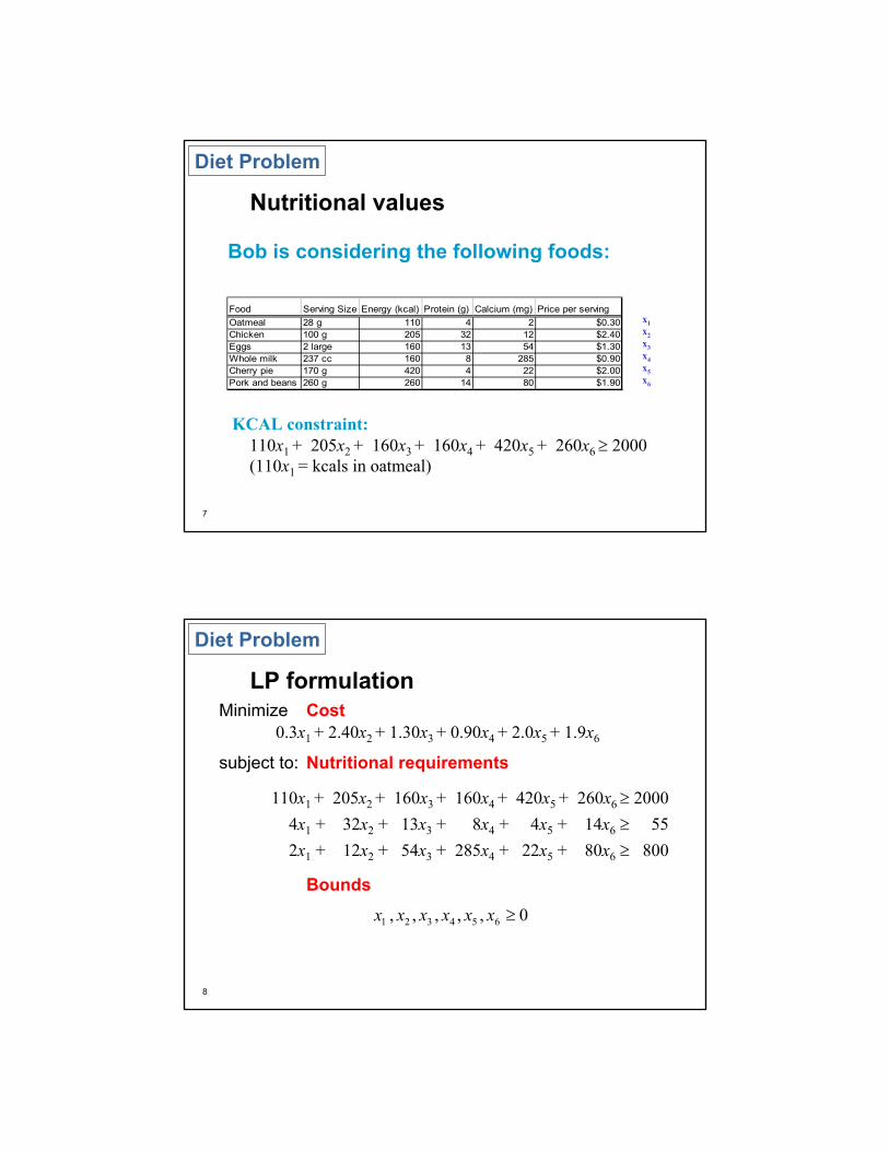
Nutritional values
Diet Problem
Bob is considering the following foods:
Food Serving Size Energy (kcal) Protein (g) Calcium (mg) Price per servingOatmeal 28 g 110 4 2 $0.30Chicken 100 g 205 32 12 $2.40Eggs 2 large 160 13 54 $1.30Whole milk 237 cc 160 8 285 $0.90Cherry pie 170 g 420 4 22 $2.00Pork and beans 260 g 260 14 80 $1.90
x1x2x3x4x5x6
KCAL constraint:110x1 + 205x2 + 160x3 + 160x4 + 420x5 + 260x6 ≥ 2000(110x1 = kcals in oatmeal)
8
LP formulation
Diet Problem
110x1 + 205x2 + 160x3 + 160x4 + 420x5 + 260x6 ≥ 20004x1 + 32x2 + 13x3 + 8x4 + 4x5 + 14x6 ≥ 552x1 + 12x2 + 54x3 + 285x4 + 22x5 + 80x6 ≥ 800
Minimize
subject to:
0,,,,, 654321 ≥xxxxxx
Cost
Nutritional requirements
Bounds
0.3x1 + 2.40x2 + 1.30x3 + 0.90x4 + 2.0x5 + 1.9x6
15 September 2003
INFORMS Practice 2002 5
9
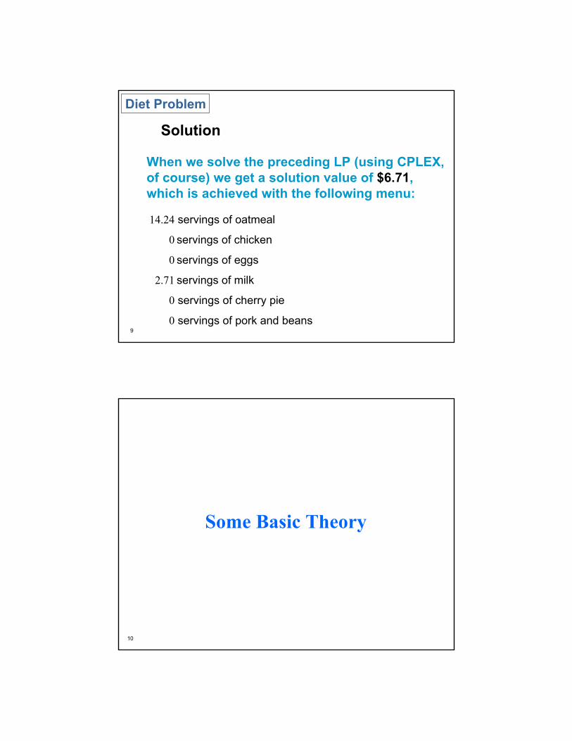
Solution
Diet Problem
When we solve the preceding LP (using CPLEX, of course) we get a solution value of $6.71, which is achieved with the following menu:
14.24 servings of oatmeal
0 servings of chicken
0 servings of eggs
2.71 servings of milk
0 servings of cherry pie
0 servings of pork and beans
10
Some Basic Theory
15 September 2003
INFORMS Practice 2002 6
11
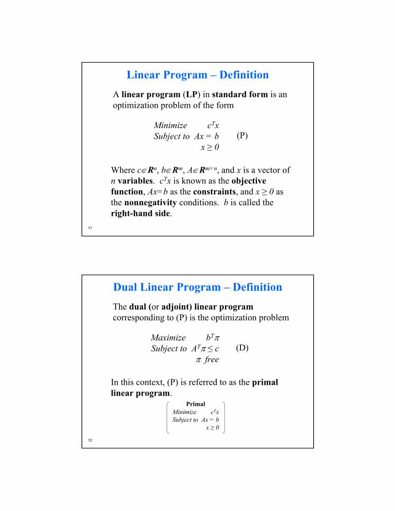
Where c∈Rn, b∈Rm, A∈Rm×n, and x is a vector of n variables. cTx is known as the objective function, Ax=b as the constraints, and x ≥ 0 as the nonnegativity conditions. b is called the right-hand side.
(P)Minimize cTxSubject to Ax = b
x ≥ 0
A linear program (LP) in standard form is an optimization problem of the form
Linear Program – Definition
12
In this context, (P) is referred to as the primal linear program.
(D)Maximize bTπSubject to ATπ ≤ c
π free
The dual (or adjoint) linear programcorresponding to (P) is the optimization problem
Minimize cTxSubject to Ax = b
x ≥ 0
Primal
Dual Linear Program – Definition
15 September 2003
INFORMS Practice 2002 7
13
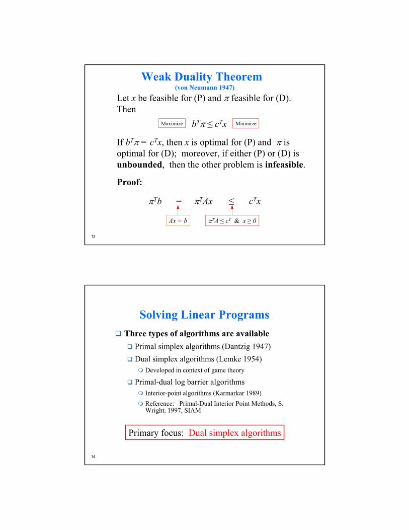
If bTπ = cTx, then x is optimal for (P) and π is optimal for (D); moreover, if either (P) or (D) is unbounded, then the other problem is infeasible.
bTπ ≤ cTx
Let x be feasible for (P) and π feasible for (D). Then
Weak Duality Theorem (von Neumann 1947)
Proof:
πTAxπTb =
Ax = b
≤ cTx
πTA ≤ cT & x ≥ 0
MinimizeMaximize
�
14
Solving Linear ProgramsThree types of algorithms are available
Primal simplex algorithms (Dantzig 1947)Dual simplex algorithms (Lemke 1954)
Developed in context of game theory
Primal-dual log barrier algorithmsInterior-point algorithms (Karmarkar 1989)Reference: Primal-Dual Interior Point Methods, S. Wright, 1997, SIAM
Primary focus: Dual simplex algorithms
15 September 2003
INFORMS Practice 2002 8
15
Basic Solutions – Definition
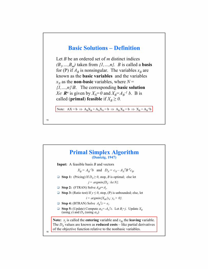
Let B be an ordered set of m distinct indices (B1,…,Bm) taken from {1,…,n}. B is called a basisfor (P) if AB is nonsingular. The variables xB are known as the basic variables and the variables xN as the non-basic variables, where N = {1,…,n}\B. The corresponding basic solutionX∈ Rn is given by XN=0 and XB=AB
-1 b. B is called (primal) feasible if XB ≥ 0.
Note: AX = b ⇒ ABXB + ANXN = b ⇒ AB XB = b ⇒ XB = AB-1b
16
Primal Simplex Algorithm(Dantzig, 1947)
Input: A feasible basis B and vectors XB = AB
-1b and DN = cN – ANTB-TcB.
Step 1: (Pricing) If DN ≥ 0, stop, B is optimal; else let j = argmin{Dk : k∈N}.
Step 2: (FTRAN) Solve ABy=Aj.Step 3: (Ratio test) If y ≤ 0, stop, (P) is unbounded; else, let
i = argmin{XBk/yk: yk > 0}.Step 4: (BTRAN) Solve AB
Tz = ei.Step 5: (Update) Compute αN=-AN
Tz. Let Bi=j. Update XB(using y) and DN (using αN)
Note: xj is called the entering variable and xBi the leaving variable. The DN values are known as reduced costs – like partial derivatives of the objective function relative to the nonbasic variables.
15 September 2003
INFORMS Practice 2002 9
17
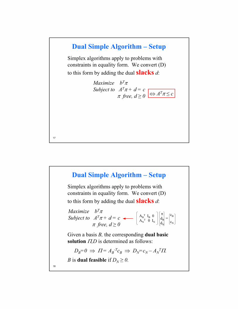
Dual Simple Algorithm – SetupSimplex algorithms apply to problems with constraints in equality form. We convert (D) to this form by adding the dual slacks d:
Maximize bTπSubject to ATπ + d = c
π free, d ≥ 0 ⇔ ATπ ≤ c
18
Dual Simple Algorithm – SetupSimplex algorithms apply to problems with constraints in equality form. We convert (D) to this form by adding the dual slacks d:
Maximize bTπSubject to ATπ + d = c
π free, d ≥ 0
Given a basis B, the corresponding dual basicsolution Π,D is determined as follows:
DB=0 ⇒ Π = AB-TcB ⇒ DN=cN – AN
TΠ.
B is dual feasible if DN ≥ 0.
=ABT IB 0
ANT 0 IN
πdBdN
cB
cN
15 September 2003
INFORMS Practice 2002 10
19
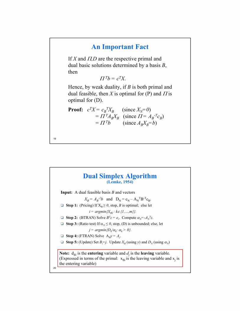
An Important FactIf X and Π,D are the respective primal and dual basic solutions determined by a basis B, then
Π Tb = cTX.Hence, by weak duality, if B is both primal and dual feasible, then X is optimal for (P) and Π is optimal for (D).
Proof: cTX = cBTXB (since XN=0)
= Π TABXB (since Π = AB-TcB)
= Π Tb (since ABXB=b) �
20
Dual Simplex Algorithm(Lemke, 1954)
Input: A dual feasible basis B and vectors XB = AB
-1b and DN = cN – ANTB-TcB.
Step 1: (Pricing) If XB≥ 0, stop, B is optimal; else leti = argmin{XBk : k∈{1,…,m}}.
Step 2: (BTRAN) Solve BTz = ei. Compute αN=-ANTz.
Step 3: (Ratio test) If αN ≤ 0, stop, (D) is unbounded; else, let j = argmin{Dk/αk: αk > 0}.
Step 4: (FTRAN) Solve ABy = Aj.Step 5: (Update) Set Bi=j. Update XB (using y) and DN (using αN)
Note: dBi is the entering variable and dj is the leaving variable. (Expressed in terms of the primal: xBi is the leaving variable and xj is the entering variable)
15 September 2003
INFORMS Practice 2002 11
21
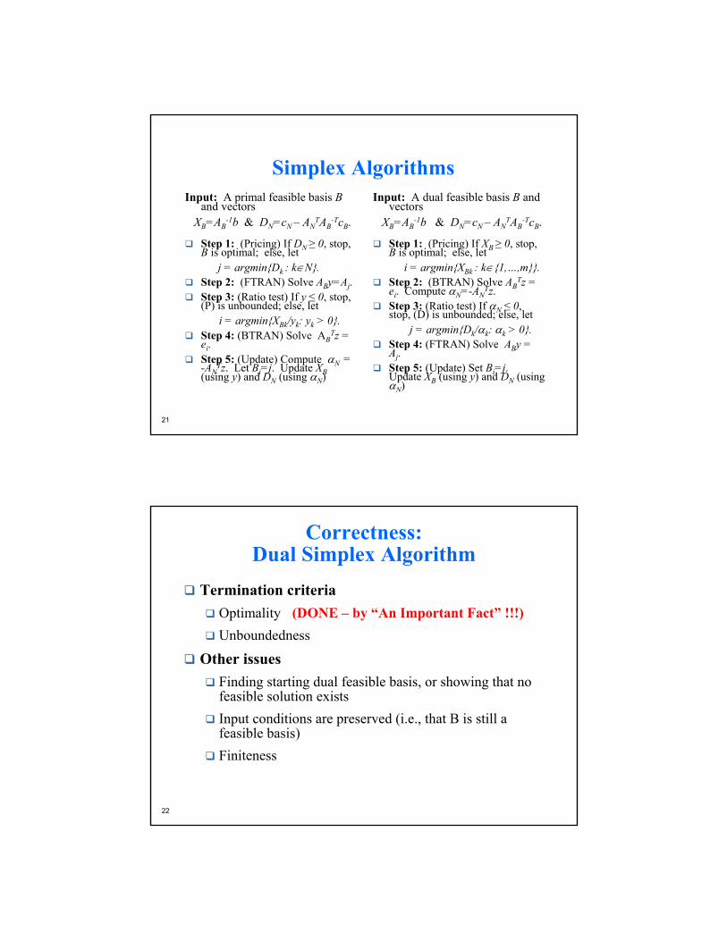
Simplex AlgorithmsInput: A primal feasible basis B
and vectors XB=AB
-1b & DN=cN – ANTAB
-TcB.
Step 1: (Pricing) If DN ≥ 0, stop, B is optimal; else, let
j = argmin{Dk : k∈N}.Step 2: (FTRAN) Solve ABy=Aj.Step 3: (Ratio test) If y ≤ 0, stop, (P) is unbounded; else, let
i = argmin{XBk/yk: yk > 0}.Step 4: (BTRAN) Solve AB
Tz = ei.Step 5: (Update) Compute αN = -AN
Tz. Let Bi=j. Update XB(using y) and DN (using αN)
Input: A dual feasible basis B and vectors
XB=AB-1b & DN=cN – AN
TAB-TcB.
Step 1: (Pricing) If XB ≥ 0, stop, B is optimal; else, let
i = argmin{XBk : k∈{1,…,m}}.Step 2: (BTRAN) Solve AB
Tz = ei. Compute αN=-AN
Tz.Step 3: (Ratio test) If αN ≤ 0, stop, (D) is unbounded; else, let
j = argmin{Dk/αk: αk > 0}.Step 4: (FTRAN) Solve ABy = Aj.Step 5: (Update) Set Bi=j. Update XB (using y) and DN (using αN)
22
Correctness: Dual Simplex Algorithm
Termination criteriaOptimalityUnboundedness
Other issuesFinding starting dual feasible basis, or showing that no feasible solution existsInput conditions are preserved (i.e., that B is still a feasible basis)Finiteness
(DONE – by “An Important Fact” !!!)
15 September 2003
INFORMS Practice 2002 12
23
Summary:What we have done and what we have to do
DoneDefined primal and dual linear programsProved the weak duality theoremIntroduced the concept of a basisStated primal and dual simplex algorithms
To do (for dual simplex algorithm)Show correctnessDescribe key implementation ideasMotivate
24
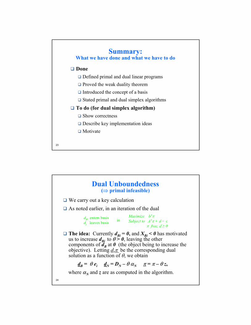
Dual Unboundedness(⇒ primal infeasible)
We carry out a key calculationAs noted earlier, in an iteration of the dual
The idea: Currently dBi = 0, and XBi < 0 has motivated us to increase dBi to θ > 0, leaving the other components of dB at 0 (the object being to increase the objective). Letting d,π be the corresponding dual solution as a function of θ, we obtain
dB = θ ei dN = DN – θ αN π = π – θ z,where αN and z are as computed in the algorithm.
dBi enters basisdj leaves basis in
Maximize bTπSubject to ATπ + d = c
π free, d ≥ 0
15 September 2003
INFORMS Practice 2002 13
25
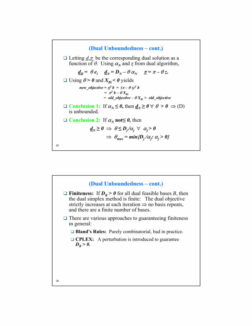
(Dual Unboundedness – cont.)
Letting d,π be the corresponding dual solution as a function of θ. Using αN and z from dual algorithm,
dB = θ ei dN = DN – θ αN π = π – θ z.Using θ > 0 and XBi < 0 yields
new_objective = πT b = (π – θ z)T b = πT b – θ XBi= old_objective – θ XBi > old_objective
Conclusion 1: If αN ≤ 0, then dN ≥ 0 ∀ θ > 0 ⇒ (D) is unbounded.Conclusion 2: If αN not≤ 0, then
dN ≥ 0 ⇒ θ ≤ Dj /αj ∀ αj > 0 ⇒ θmax = min{Dj /αj: αj > 0}
26
(Dual Unboundedness – cont.)
Finiteness: If DB > 0 for all dual feasible bases B, then the dual simplex method is finite: The dual objective strictly increases at each iteration ⇒ no basis repeats, and there are a finite number of bases.There are various approaches to guaranteeing finiteness in general:
Bland’s Rules: Purely combinatorial, bad in practice.CPLEX: A perturbation is introduced to guarantee DB > 0.
15 September 2003
INFORMS Practice 2002 14
27
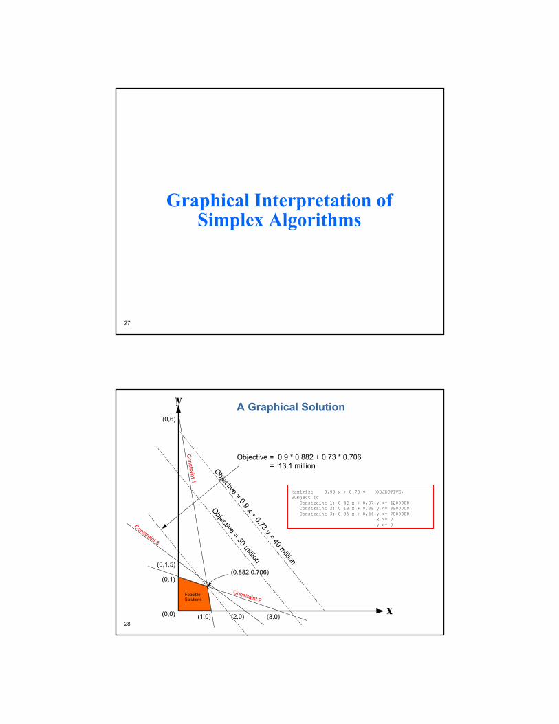
Graphical Interpretation of Simplex Algorithms
28
x
y
(0.882,0.706)
Objective = 0.9 x + 0.73 y = 40 million
Objective = 30 million
FeasibleSolutions
Objective = 0.9 * 0.882 + 0.73 * 0.706= 13.1 million
(0,6)
(1,0)
Constraint 1
(0,1)
(3,0)
Constraint 2
(0,1.5)
(2,0)
Constraint 3
A Graphical Solution
(0,0)
Maximize 0.90 x + 0.73 y (OBJECTIVE)Subject To
Constraint 1: 0.42 x + 0.07 y <= 4200000Constraint 2: 0.13 x + 0.39 y <= 3900000Constraint 3: 0.35 x + 0.44 y <= 7000000
x >= 0y >= 0
15 September 2003
INFORMS Practice 2002 15
29
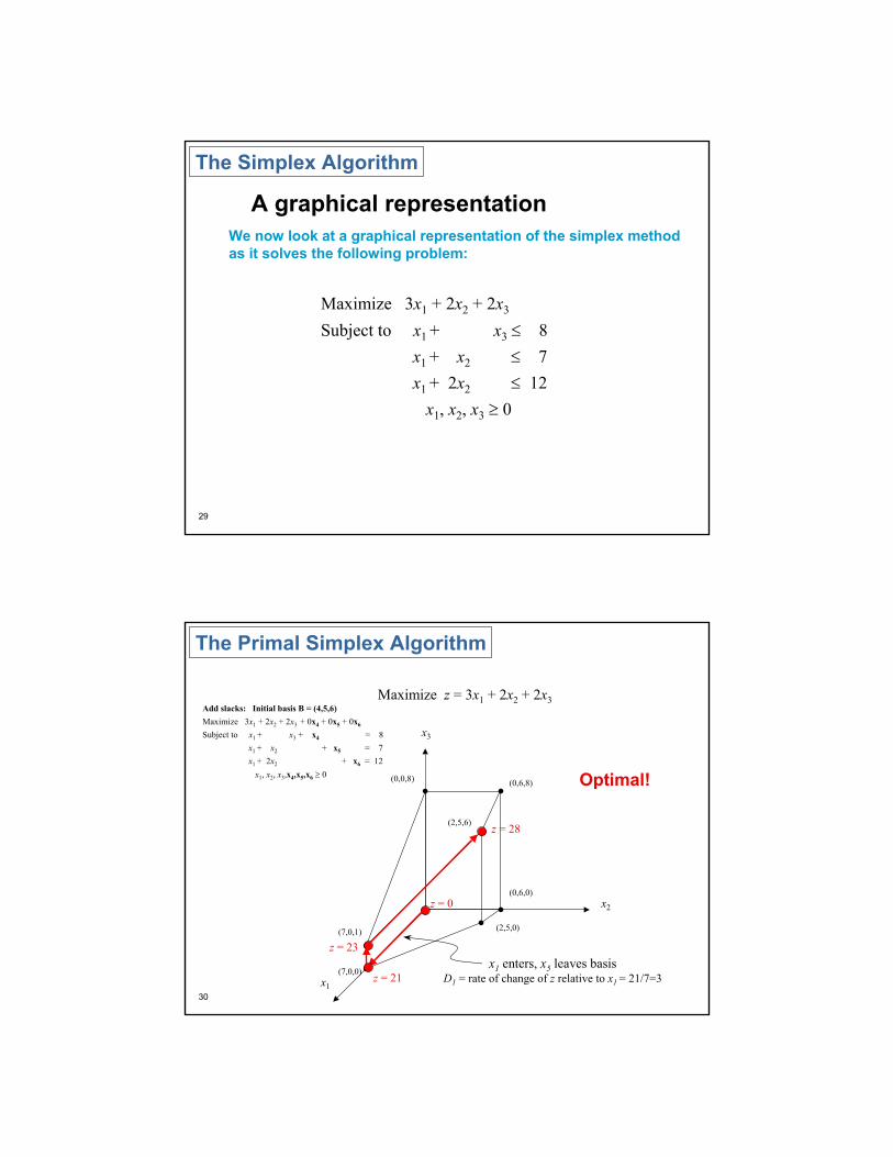
A graphical representation
The Simplex Algorithm
We now look at a graphical representation of the simplex method as it solves the following problem:
Maximize 3x1 + 2x2 + 2x3
Subject to x1 + x3 ≤ 8x1 + x2 ≤ 7x1 + 2x2 ≤ 12
x1, x2, x3 ≥ 0
30
The Primal Simplex Algorithm
x1
x2
x3
(0,0,8) (0,6,8)
(2,5,6)
(0,6,0)
(2,5,0)(7,0,1)
(7,0,0)
Maximize z = 3x1 + 2x2 + 2x3
z = 0
z = 21
z = 23
Optimal!
z = 28
Add slacks: Initial basis B = (4,5,6)Maximize 3x1 + 2x2 + 2x3 + 0x4 + 0x5 + 0x6
Subject to x1 + x3 + x4 = 8x1 + x2 + x5 = 7x1 + 2x2 + x6 = 12
x1, x2, x3,x4,x5,x6 ≥ 0
x1 enters, x5 leaves basisD1 = rate of change of z relative to x1 = 21/7=3
15 September 2003
INFORMS Practice 2002 16
31
Computational History of
Linear Programming
32
“A certain wide class of practical problems appears to be just beyond the range of modern computing machinery. These problems occur in everyday life; they run the gamut from some very simple situations that confront an individual to those connected with the national economy as a whole. Typically, these problems involve a complex of different activities in which one wishes to know which activities to emphasize in order to carry out desired objectives under known limitations.”
George B. Dantzig, 1948
15 September 2003
INFORMS Practice 2002 17
33
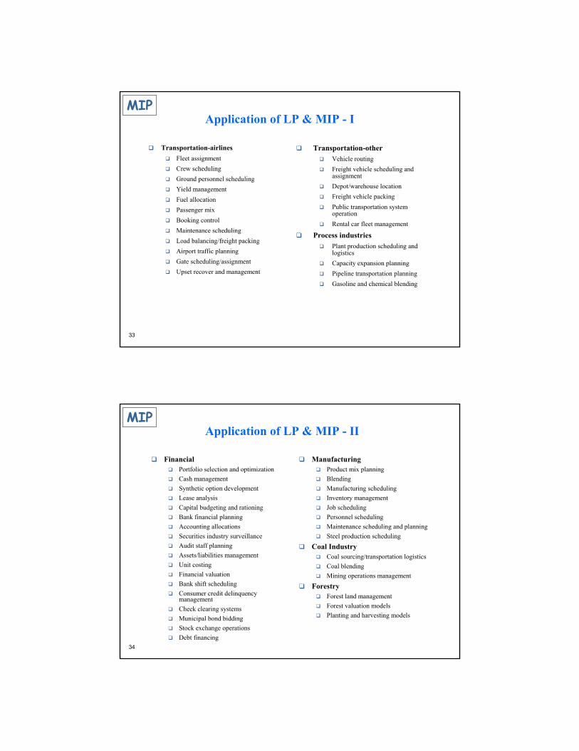
Application of LP & MIP - I
Transportation-airlinesFleet assignmentCrew schedulingGround personnel schedulingYield management Fuel allocationPassenger mixBooking controlMaintenance schedulingLoad balancing/freight packingAirport traffic planningGate scheduling/assignmentUpset recover and management
Transportation-otherVehicle routingFreight vehicle scheduling and assignmentDepot/warehouse locationFreight vehicle packingPublic transportation system operationRental car fleet management
Process industriesPlant production scheduling and logisticsCapacity expansion planningPipeline transportation planningGasoline and chemical blending
MIP
34
Application of LP & MIP - II
FinancialPortfolio selection and optimizationCash managementSynthetic option developmentLease analysisCapital budgeting and rationingBank financial planningAccounting allocationsSecurities industry surveillanceAudit staff planningAssets/liabilities managementUnit costingFinancial valuationBank shift schedulingConsumer credit delinquency managementCheck clearing systemsMunicipal bond biddingStock exchange operationsDebt financing
ManufacturingProduct mix planningBlendingManufacturing scheduling Inventory managementJob schedulingPersonnel schedulingMaintenance scheduling and planningSteel production scheduling
Coal IndustryCoal sourcing/transportation logisticsCoal blendingMining operations management
ForestryForest land managementForest valuation modelsPlanting and harvesting models
MIP
15 September 2003
INFORMS Practice 2002 18
35
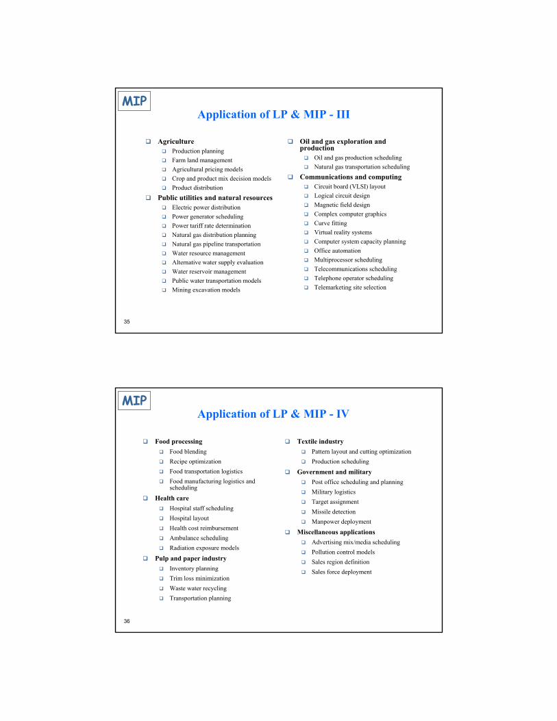
Application of LP & MIP - III
AgricultureProduction planningFarm land managementAgricultural pricing modelsCrop and product mix decision modelsProduct distribution
Public utilities and natural resourcesElectric power distributionPower generator schedulingPower tariff rate determinationNatural gas distribution planningNatural gas pipeline transportationWater resource managementAlternative water supply evaluationWater reservoir managementPublic water transportation modelsMining excavation models
Oil and gas exploration and production
Oil and gas production schedulingNatural gas transportation scheduling
Communications and computingCircuit board (VLSI) layoutLogical circuit designMagnetic field designComplex computer graphicsCurve fittingVirtual reality systemsComputer system capacity planningOffice automationMultiprocessor schedulingTelecommunications schedulingTelephone operator schedulingTelemarketing site selection
MIP
36
Application of LP & MIP - IV
Food processingFood blendingRecipe optimization Food transportation logisticsFood manufacturing logistics and scheduling
Health careHospital staff schedulingHospital layoutHealth cost reimbursementAmbulance schedulingRadiation exposure models
Pulp and paper industryInventory planningTrim loss minimizationWaste water recyclingTransportation planning
Textile industryPattern layout and cutting optimization Production scheduling
Government and militaryPost office scheduling and planningMilitary logisticsTarget assignmentMissile detectionManpower deployment
Miscellaneous applicationsAdvertising mix/media schedulingPollution control modelsSales region definitionSales force deployment
MIP
15 September 2003
INFORMS Practice 2002 19
37
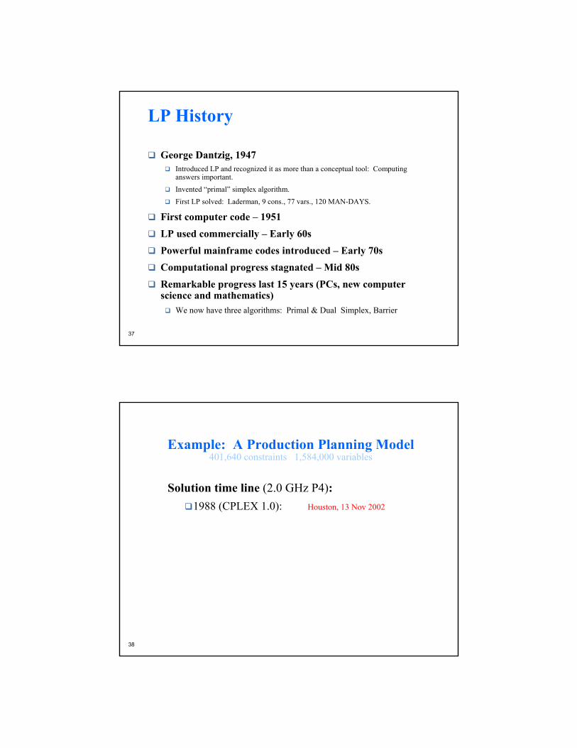
LP History
George Dantzig, 1947Introduced LP and recognized it as more than a conceptual tool: Computing answers important.Invented “primal” simplex algorithm.First LP solved: Laderman, 9 cons., 77 vars., 120 MAN-DAYS.
First computer code – 1951LP used commercially – Early 60sPowerful mainframe codes introduced – Early 70sComputational progress stagnated – Mid 80sRemarkable progress last 15 years (PCs, new computer science and mathematics)
We now have three algorithms: Primal & Dual Simplex, Barrier
38
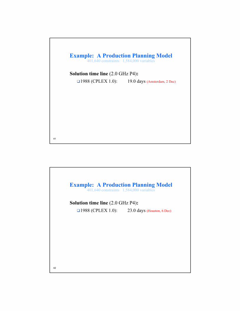
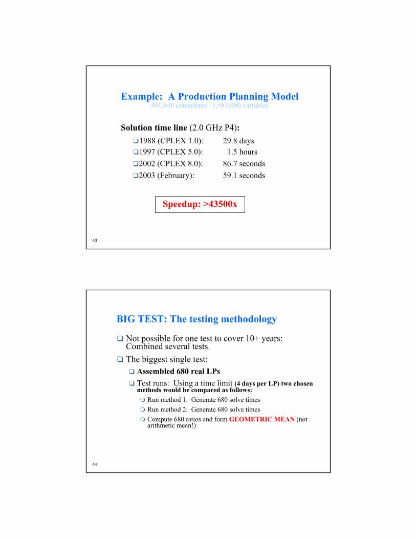
Example: A Production Planning Model401,640 constraints 1,584,000 variables
Solution time line (2.0 GHz P4):1988 (CPLEX 1.0): Houston, 13 Nov 2002
15 September 2003
INFORMS Practice 2002 20
39
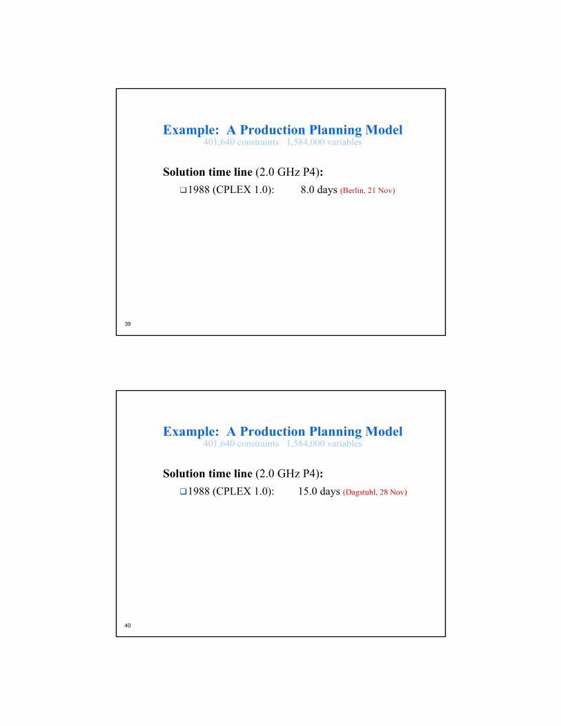
Example: A Production Planning Model401,640 constraints 1,584,000 variables
Solution time line (2.0 GHz P4):1988 (CPLEX 1.0): 8.0 days (Berlin, 21 Nov)
40
Example: A Production Planning Model401,640 constraints 1,584,000 variables
Solution time line (2.0 GHz P4):1988 (CPLEX 1.0): 15.0 days (Dagstuhl, 28 Nov)
15 September 2003
INFORMS Practice 2002 21
41
Example: A Production Planning Model401,640 constraints 1,584,000 variables
Solution time line (2.0 GHz P4):1988 (CPLEX 1.0): 19.0 days (Amsterdam, 2 Dec)
42
Example: A Production Planning Model401,640 constraints 1,584,000 variables
Solution time line (2.0 GHz P4):1988 (CPLEX 1.0): 23.0 days (Houston, 6 Dec)
15 September 2003
INFORMS Practice 2002 22
43
Example: A Production Planning Model401,640 constraints 1,584,000 variables
Solution time line (2.0 GHz P4):1988 (CPLEX 1.0): 29.8 days
Speedup: >43500x
1997 (CPLEX 5.0): 1.5 hours2002 (CPLEX 8.0): 86.7 seconds2003 (February): 59.1 seconds
44
BIG TEST: The testing methodology
Not possible for one test to cover 10+ years: Combined several tests.The biggest single test:
Assembled 680 real LPsTest runs: Using a time limit (4 days per LP) two chosen methods would be compared as follows:
Run method 1: Generate 680 solve timesRun method 2: Generate 680 solve timesCompute 680 ratios and form GEOMETRIC MEAN (not arithmetic mean!)
15 September 2003
INFORMS Practice 2002 23
45
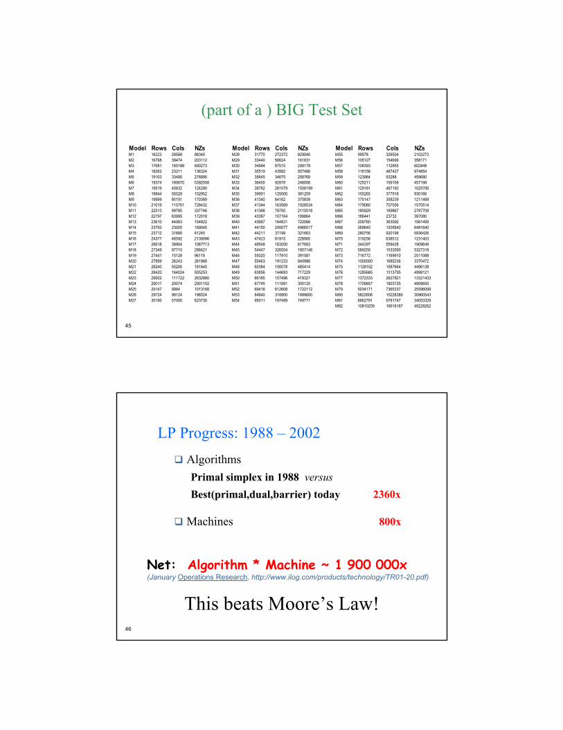
(part of a ) BIG Test Set
Model Rows Cols NZs Model Rows Cols NZs Model Rows Cols NZsM1 16223 28568 88340 M28 31770 272372 829040 M55 99578 326504 2102273M2 16768 39474 203112 M29 33440 56624 161831 M56 105127 154699 358171M3 17681 165188 690273 M30 34994 87510 208179 M57 108393 112955 602948M4 18262 23211 136324 M31 35519 43582 557466 M58 118158 487427 974854M5 19103 33490 276895 M32 35645 34675 208769 M59 123964 93288 459680M6 19374 180670 5392558 M33 36400 92878 246006 M60 125211 159109 457198M7 19519 45832 124280 M34 38782 261079 1508199 M61 129181 467192 1025706M8 19844 55528 152952 M35 39951 125000 381259 M62 155265 377918 930166M9 19999 85191 170369 M36 41340 64162 370839 M63 175147 358239 1211488M10 21019 115761 728432 M37 41344 163569 1928534 M64 179080 707556 1570514M11 22513 99785 337746 M38 41366 78750 2110518 M65 185929 189867 2787708M12 22797 63995 172018 M39 43387 107164 189864 M66 186441 23732 397080M13 23610 44063 154822 M40 43687 164831 722066 M67 209760 363092 1061495M14 23700 23005 169045 M41 44150 200077 4966017 M68 269640 1205640 6481640M15 23712 31680 81245 M42 44211 37199 321663 M69 280756 920198 5936426M16 24377 46592 2139096 M43 47423 81915 228565 M70 319256 638512 1231403M17 26618 38904 1067713 M44 48548 163200 617683 M71 344297 559428 1909649M18 27349 97710 288421 M45 54447 326504 1807146 M72 589250 1533590 5327318M19 27441 15128 96118 M46 55020 117910 391081 M73 716772 1169910 2511088M20 27899 26243 261968 M47 55463 191233 840986 M74 1000000 1685236 3370472M21 28240 55200 161640 M48 60384 100078 485414 M75 1128152 1587664 4496138M22 28420 164024 505253 M49 63856 144693 717229 M76 1285665 1313795 4998121M23 29002 111722 2632880 M50 66185 157496 418321 M77 1372333 2627821 13321433M24 29017 20074 2001102 M51 67745 111891 305125 M78 1709857 1903725 4959650M25 29147 9984 1013168 M52 69418 612608 1722112 M79 5034171 7365337 25596099M26 29724 98124 196524 M53 84840 316800 1899600 M80 5822606 15228380 30960543M27 30190 57000 623730 M54 95011 197489 749771 M81 6662791 9781747 34053329
M82 10810259 19916187 49228262
46
LP Progress: 1988 – 2002AlgorithmsPrimal simplex in 1988 versusBest(primal,dual,barrier) today 2360x
Machines 800x
Net: Algorithm * Machine ~ 1 900 000x(January Operations Research, http://www.ilog.com/products/technology/TR01-20.pdf)
This beats Moore’s Law!
15 September 2003
INFORMS Practice 2002 24
47
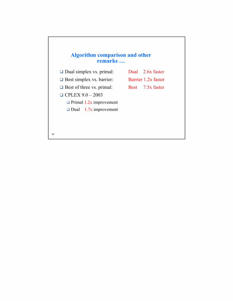
Algorithm comparison and other remarks …
Dual simplex vs. primal: Dual 2.6x fasterBest simplex vs. barrier: Barrier 1.2x fasterBest of three vs. primal: Best 7.5x fasterCPLEX 9.0 – 2003
Primal 1.2x improvementDual 1.7x improvement


![AN ALGORITHM FOR SOLVING THE LINEAR INTEGER PROGRAMMING ... · whereupon (l) represents a pure integer programming problem. Following Gomory [5], if we relax the requirement z i 0,](https://img.pdfslide.us/doc/110x75/5f38a48d4e895f192e3b51d3/an-algorithm-for-solving-the-linear-integer-programming-whereupon-l-represents.jpg)