Embed Size (px)
Citation preview
Solving Dynamic Models with Heterogeneous Agents and
Aggregate Uncertainty with Dynare or Dynare++
Wouter J. DEN HAAN and Tarık Sezgin OCAKTAN ∗
June 10, 2009
Abstract
This paper shows how models with heterogeneous agents and aggregate uncertainty
can be solved using Dynare or Dynare++ software that implements a perturbation
approach. When the explicit aggregation algorithm (XPA) is used to obtain aggre-
gate laws of motion, this can be accomplished by combining a Dynare program with
a very simple Matlab program. When the Krusell-Smith algorithm is used, then the
Matlab program needed is somewhat more involved, but still relatively simple. We
calculate and compare 1st and 2nd-order numerical solutions using both algorithms.
These numerical procedures are also compared with the algorithm that solves the indi-
vidual policy rules with a projection instead of a perturbation procedure. Finally, we
discuss a procedure that efficiently chooses which cross-sectional moments to include
as aggregate state variables when nonlinearities are important and the mean is not a
sufficient statistic.
Key Words : numerical solutions, projection methods
JEL Classification: C63, D52
∗den Haan: University of Amsterdam and CEPR, e-mail: [email protected]; Ocaktan: Paris School of
Economics, email: [email protected]. We would like to thank Michel Juillard, Christophe Cahn and
Markus Kirchner
Introduction
The most populair model in macroeconomics is the New Keynesian model. There are
many quite sophisticated versions of this model, but most of them rely on the represen-
tative agent paradigm. If there are heterogeneous agents in the model, then the degree
of heterogeneity is limited, for example, by just having two representative agents, like a
patient and an impatient agent. The assumptions needed to justify a representative agent
framework, like perfect insurance of idiosyncratic risk, are believed to be unrealistic. Even
if there are representative agent models that can describe the aggregate economy well,
they obviously cannot explain any distributional aspects, although these are of interest
to many economists. Fortunately, there are now numerous papers in which heterogeneity
and idiosyncratic risk play a key role. There are even quite a few papers in which there is
both heterogeneity and aggregate risk, a combination that makes it more cumbersome to
obtain a numerical solution. Nevertheless, the overwhelming majority of papers still relies
on models with a representative agent.
An important reason for the ongoing dominance of models with a representative agent
is without doubt the availability of user friendly software, like Dynare, to solve and esti-
mate these types of models. In principle Dynare can handle many state variables and, thus,
should be able to solve models with multiple agents. The problem is that in macroeco-
nomic models we would like to have millions of agents and such a large number of agents is
problematic, even for Dynare.1 The standard assumption is to approximate these millions
of agents with a continuum of agents, but Dynare requires a finite number.
In this paper, we show how to use Dynare to solve models with (i) a continuum of
heterogeneous agents and (ii) aggregate risk. Two things are needed. First, a ”mother”
program is needed to solve for the laws of motion that describe the aggregate variables
taking as given the solution of the individual policy rules. Second, a Dynare program is
needed to solve for the individual policy rules taking as given the aggregate law of motion.
1An interesting question is whether using a relatively small number, say 100, is enough to approximate
a macroeconomy with millions of agents. It would be cumbersome to use Dynare to solve models with 100
agents, but this is likely to be feasible at least for some models and for lower-order perturbation solutions.
1
This Dynare program, the *.mod file, needs to be able to read the coefficients of the
aggregate law of motion. We show that this can be accomplished with an easy procedure
for a Dynare program and with a somewhat more cumbersome procedure for a Dynare++
program.
Preston and Roca (2006) were the first to realize that one can use perturbation tech-
niques to solve models with a continuum of heterogeneous agents and aggregate risk. den
Haan and Rendahl (2009) develop the XPA algorithm with which aggregate laws of motion
are obtained by explicitly aggregating the individual policy rules, even when the individ-
ual policy rules are not linear. In the algorithm of den Haan and Rendahl (2009), the
individual policy rules can be obtained with any algorithm. In this paper, we show that
if the individual policy rules are obtained with perturbation techniques, that the XPA so-
lution is identical to the one obtained by the algorithm of Preston and Roca (2006). The
advantage of the XPA algorithm is the simplicity and transparency and this approach is
used here to write the programs.
What is required to be able to implement XPA with Dynare? The Dynare program
itself, that solves for the individual laws of motion would be almost a standard Dynare
program. However it differs from a standard Dynare program in two aspects. First,
as explained above it needs to be able to incorporate the values of the coefficients of the
aggregate laws of motion. The second modification is related to the feature of XPA that to
be able to explicitly aggregate higher-order individual policy functions you need auxiliary
policy rules. For example, if the model has a policy rule for the capital choice, k, then
one needs an auxiliary policy rule for k2 if a second-order perturbation solution is used.
But this would just boil down to adding one variable and one equation to the standard
Dynare file. The mother program would be very simple. There are two parts to the
mother program. First, it would contain a few steps of algebra to get the coefficients of
the aggregate laws of motion from the individual laws of motion. Second, it has to contain
a procedure to make the laws of motion of the aggregate variables consistent with the
laws of motion of the individual variables. For example, one can start with an aggregate
policy rule, solve for the individual policy rule using perturbation techniques, obtain the
2
aggregate law of motion by explicit aggregation of the individual policy rule, and iterate
until the aggregate law of motion has converged. But there are better, more efficient,
ways of obtaining the consistency and we’ll discuss how to write the mother program to
implement them.
We use this algorithm to generate first and second-order solutions. We assess the
accuracy and compare the solutions with those obtained with alternative algorithms. The
first alternative algorithm uses the same Dynare program to solve for the individual policy
rules, but obtains the aggregate law using the simulation procedure proposed by Krusell
and Smith (1998) instead of explicit aggregation. The mother program is then a bit more
complicated, because it has to include a simulation procedure, but the structure of the
program remains the same. We also consider an algorithm in which the aggregate laws of
motion are still solved by explicit aggregation, but the individual policy rules are obtained
using a projection method. Given that there is no standard software (yet) to implement
projection methods, this procedure is obviously much more involved than any of the others
considered.
The main contributions of this paper are (i) to establish the link between the algorithm
of Preston and Roca (2006) and the XPA algorithm of den Haan and Rendahl (2009), (ii)
describe how Dynare and Dynare++ can be used to implement these algorithms, and (iii)
compare the different numerical solutions and access their accuracy. Finally, there is one
more important issue that is addressed in this paper and that describing a procedure to
limit the number of state variables. In several models considered so far, the computational
burden turns out to be low, because only a small set of moments, in fact typically just the
mean, is sufficient to capture the predictive information in the distribution, a property
referred to as approximate aggregation.2 This is not likely to be a universal property. Key
for approximate aggregation to hold is that the individual policy functions are close to
being linear in the relevant part of the state space.3 Linear policy rules are unlikely to be
a realistic property in general and it is (hopefully) only a matter of time in which we will
2See Krusell and Smith (2006).3For example, nonlinearities do not matter for the very poor agents because their behavior is not
important for the aggregate anyway.
3
use models in which nonlinearities matter for aggregation. But if nonlinearities matter,
then additional moments have to be used as state variables. Strictly following the logic of
the XPA algorithm implies that each non-linear basis term used in the individual policy
function gives rise to an additional cross-sectional moment in the set of state variables.
We show how to reduce the dimension of this set by using combinations of these state
variables. This contribution is likely to be more important when the individual policy
rules are solved with a projection procedure than with a perturbation procedure given
that it is tricky to keep the cost of projection methods low with a large number of state
variables.
1 The Model
In this section we describe the model which is a standard heterogeneous agents model with
aggregate productivity shocks similar to the one discussed in Aiyagari (1994), Bewley (un-
dated) and Huggett (1993). It describes a simple exchange economy with incomplete mar-
kets, aggregate uncertainty and an infinite number of agents. The source of heterogeneity
comes from the assumption that there are idiosyncratic income shocks, which partially
uninsurable.
Problem for the individual agent The economy is represented by a stochastic growth
model with a continuum of individuals indexed by i ∈ [0, 1]. The individual agents are
characterized by facing an idiosyncratic unemployment risk. All agents are ex ante iden-
tical, however there is ex post heterogeneity due to incomplete insurance markets and
borrowing constraints. Every quarter individuals differ from each other through their as-
set holdings and employment opportunities. In order to transfer their ressources over time,
agents can only control their capital holdings. We simplify the model with respect to the
one described in Preston and Roca (2006), and we assume that an employed agent earns
a wage rate of w, while an unemployed agent has no income. However agents can insure
themselves, at least partially, against employment risks by building up a capital stock. To
insure satisfaction of intertemporal budget constraints, capital holdings are restricted by a
4

borrowing limit b ≥ 0, ensuring the repayment of loans and the absence of Ponzi schemes.
Agent i’s maximization problem is given by
max{cit,ai,t+1}
Et
∞∑
t=0
βt c1−γit − 1
1 − γ
s.t. cit + ai,t+1 = r(kt, lt, zt)ait + w(kt, lt, zt)eit l + (1 − δ)ait (1)
ait ≥ b
The utility function is characterized by a standard constant relative risk aversion (CRRA)
utility function with risk aversion parameter γ > 0. This function is twice continuously
differentiable, increasing, and concave in the level of consumption of household i, cit. Let
ait be the agent’s beginning-of-period asset holdings, ai,t+1 is the next period level of asset
constrained, l is the time endowment, β the subjective discount rate, 0 < δ < 1 is the
depreciation rate. rt and wt is the interest rate and wage rate, respectively.
Each agent faces partially insurable labor market income risk and is endowed with one
unit of time. This endowment is transformed into labor input according to lit = eit l. The
stochastic employment opportunity eit follows an autoregressive process of the form
ei,t+1 = (1 − ρe)µe + ρeeit + εei,t+1 , εe
t ∼ N (0, σ2e ) (2)
where 0 < ρe < 1, µe > 0 and εei,t+1 a bounded i.i.d. disturbance with mean and variance
(0, σ2e ).
Problem for the firm Markets are competitive and the production technology of the
firm is characterized by a Cobb-Douglas production function. Let kt and lt stand for per
capita capital and the employment rate, respectively. Per capita aggregate output takes
as inputs the aggregate capital stock and labor supply
yt = ztkαt l1−α
t
In the original model, as described in Krusell and Smith (1998), aggregate productivity,
zt, is an exogeneous stochastic process that can take on two values, which are interpreted
as the good and bad state of the economy. For reasons that will be described later, we
5
transform the discrete space to a continuous support by assuming that the aggregate
technology shock zt , common to all households, satisfies
zt+1 = (1 − ρz)µz + ρzzt + εzt+1 (3)
where 0 < ρz < 1, µz > 0 and εzt+1 a bounded i.i.d. disturbance with mean and variance
(0, σ2z ). We assume that firms rent their factors of production from households in compet-
itive spot markets. These aggregate inputs imply market interest and wage rates equal
to
r(kt, lt, zt) = αzt
(
kt
lt
)α−1
(4)
w(kt, lt, zt) = (1 − α)zt
(
kt
lt
)α
(5)
In order to solve the optimization program given by expression (1) agents must forecast
future prices. Under the maintained assumptions (lt, zt) follow an exogeneous stochastic
process. Therefore in order to forecast future wage and rental rates, agents must know the
stochastic process that describes the evolution of the aggregate capital stock. However, the
stochastic properties of the aggregate capital stock depend on the distribution of capital
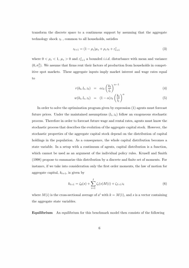
holdings in the population. As a consequence, the whole capital distribution becomes a
state variable. In a setup with a continuum of agents, capital distribution is a function,
which cannot be used as an argument of the individual policy rules. Krusell and Smith
(1998) propose to summarize this distribution by a discrete and finite set of moments. For
instance, if we take into consideration only the first order moments, the law of motion for
aggregate capital, kt+1, is given by
kt+1 = ζ0(s) +I
∑
i=1
ζi(s)M(i) + ζI+1zt (6)
where M(i) is the cross-sectional average of ai with k = M(1), and s is a vector containing
the aggregate state variables.
Equilibrium An equilibrium for this benchmark model then consists of the following
6
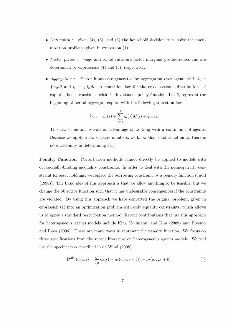
• Optimality : given (4), (5), and (6) the household decision rules solve the maxi-
mization problems given in expression (1).
• Factor prices : wage and rental rates are factor marginal productivities and are
determined by expressions (4) and (5), respectively.
• Aggregation : Factor inputs are generated by aggregation over agents with kt ≡∫
aitdi and lt ≡∫
litdi. A transition law for the cross-sectional distributions of
capital, that is consistent with the investment policy function. Let kt represent the
beginning-of-period aggregate capital with the following transition law
kt+1 = ζ0(s) +
I∑
i=1
ζi(s)M(i) + ζI+1zt
This law of motion reveals an advantage of working with a continuum of agents.
Because we apply a law of large numbers, we know that conditional on zt, there is
no uncertainty in determining kt+1
Penalty Function Perturbation methods cannot directly be applied to models with
occasionally-binding inequality constraints. In order to deal with the nonnegativity con-
straint for asset holdings, we replace the borrowing constraint by a penalty function (Judd
(1998)). The basic idea of this approach is that we allow anything to be feasible, but we
change the objective function such that it has undesirable consequences if the constraints
are violated. By using this approach we have converted the original problem, given in
expression (1) into an optimization problem with only equality constraints, which allows
us to apply a standard perturbation method. Recent contributions that use this approach
for heterogeneous agents models include Kim, Kollmann, and Kim (2009) and Preston
and Roca (2006). There are many ways to represent the penalty function. We focus on
three specifications from the recent literature on heterogeneous agents models. We will
use the specification described in de Wind (2008)
PdW (ai,t+1) =η1
η0
exp(
− η0(ai,t+1 + b))
− η2(ai,t+1 + b) (7)
7
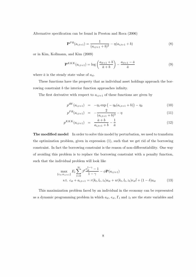
Alternative specification can be found in Preston and Roca (2006)
PPR(ai,t+1) =1
(ai,t+1 + b)2− η(ai,t+1 + b) (8)
or in Kim, Kollmann, and Kim (2009)
PKKK(ai,t+1) = log
(
ait+1 + b
a + b
)
−ait+1 − a
a(9)
where a is the steady state value of ait.
These functions have the property that as individual asset holdings approach the bor-
rowing constraint b the interior function approaches infinity.
The first derivative with respect to ai,t+1 of these functions are given by
pdW (ai,t+1) = −η1 exp(
− η0(ai,t+1 + b))
− η2 (10)
pPR(ai,t+1) = −2
(ai,t+1 + b)3− η (11)
pKKK(ai,t+1) =a + b
ai,t+1 + b−
1
a(12)
The modified model In order to solve this model by perturbation, we need to transform
the optimization problem, given in expression (1), such that we get rid of the borrowing
constraint. In fact the borrowing constraint is the reason of non-differentiability. One way
of avoiding this problem is to replace the borrowing constraint with a penalty function,
such that the individual problem will look like
max{cit,ai,t+1}
Et
∞∑
t=0
βt c1−γit − 1
1 − γ− φP(ai,t+1)
s.t. cit + ai,t+1 = r(kt, lt, zt)ait + w(kt, lt, zt)eit l + (1 − δ)ait (13)
This maximization problem faced by an individual in the economy can be represented
as a dynamic programming problem in which ait, eit, Γt and zt are the state variables and
8
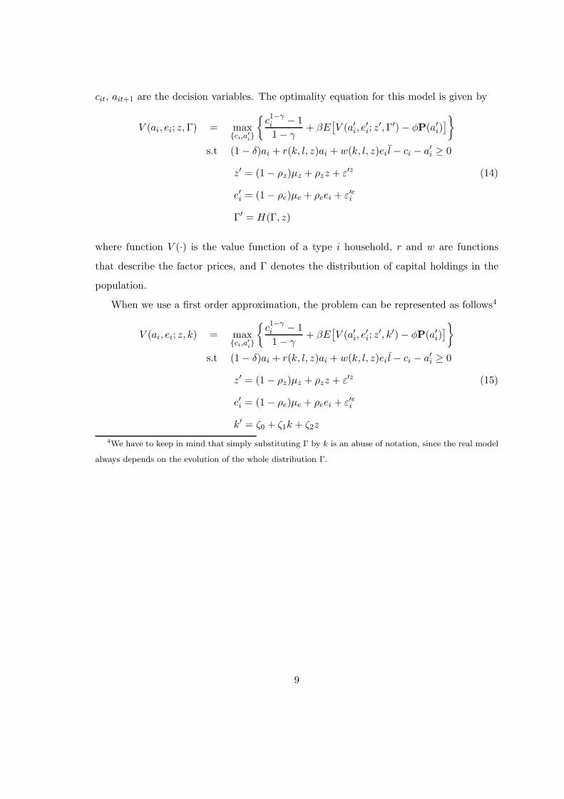
cit, ait+1 are the decision variables. The optimality equation for this model is given by
V (ai, ei; z,Γ) = max{ci,a
′
i}
{
c1−γi − 1
1 − γ+ βE
[
V (a′i, e′i; z
′,Γ′) − φP(a′i)]
}
s.t (1 − δ)ai + r(k, l, z)ai + w(k, l, z)ei l − ci − a′i ≥ 0
z′ = (1 − ρz)µz + ρzz + ε′z (14)
e′i = (1 − ρe)µe + ρeei + ε′ei
Γ′ = H(Γ, z)
where function V (·) is the value function of a type i household, r and w are functions
that describe the factor prices, and Γ denotes the distribution of capital holdings in the
population.
When we use a first order approximation, the problem can be represented as follows4
V (ai, ei; z, k) = max{ci,a
′
i}
{
c1−γi − 1
1 − γ+ βE
[
V (a′i, e′i; z
′, k′) − φP(a′i)]
}
s.t (1 − δ)ai + r(k, l, z)ai + w(k, l, z)ei l − ci − a′i ≥ 0
z′ = (1 − ρz)µz + ρzz + ε′z (15)
e′i = (1 − ρe)µe + ρeei + ε′ei
k′ = ζ0 + ζ1k + ζ2z
4We have to keep in mind that simply substituting Γ by k is an abuse of notation, since the real model
always depends on the evolution of the whole distribution Γ.
9
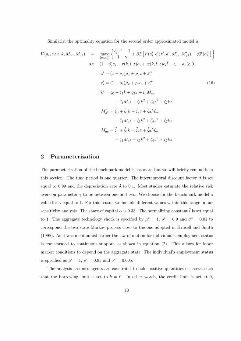
Similarly, the optimality equation for the second order approximated model is
V (ai, ei; z, k,Mae,Ma2) = max{ci,a
′
i}
{
c1−γi − 1
1 − γ+ βE
[
V (a′i, e′i; z
′, k′,M ′ae,M
′a2) − φP(a′i)
]
}
s.t (1 − δ)ai + r(k, l, z)ai + w(k, l, z)ei l − ci − a′i ≥ 0
z′ = (1 − ρz)µz + ρzz + ε′z
e′i = (1 − ρe)µe + ρeei + ε′ei (16)
k′ = ζ0 + ζ1k + ζ2z + ζ3Mae
+ ζ4Ma2 + ζ5k2 + ζ6z
2 + ζ7kz
M ′a2 = ζ0 + ζ1k + ζ2z + ζ3Mae
+ ζ4Ma2 + ζ5k2 + ζ6z
2 + ζ7kz
M ′ae = ζ0 + ζ1k + ζ2z + ζ3Mae
+ ζ4Ma2 + ζ5k2 + ζ6z
2 + ζ7kz
2 Parameterization
The parameterization of the benchmark model is standard but we will briefly remind it in
this section. The time period is one quarter. The intertemporal discount factor β is set
equal to 0.99 and the depreciation rate δ to 0.1. Most studies estimate the relative risk
aversion parameter γ to be between one and two. We choose for the benchmark model a
value for γ equal to 1. For this reason we include different values within this range in our
sensitivity analysis. The share of capital α is 0.33. The normalizing constant l is set equal
to 1. The aggregate technology shock is specified by µz = 1, ρz = 0.9 and σz = 0.01 to
correspond the two state Markov process close to the one adopted in Krusell and Smith
(1998). As it was mentionned earlier the law of motion for individual’s employment status
is transformed to continuous support, as shown in equation (2). This allows for labor
market conditions to depend on the aggregate state. The individual’s employment status
is specified as µe = 1, ρe = 0.95 and σe = 0.005.
The analysis assumes agents are constraint to hold positive quantities of assets, such
that the borrowing limit is set to b = 0. In other words, the credit limit is set at 0,
10
which means that agents are not allowed to hold net debt. The parameter φ controls
the sensitivity to the borrowing constraint in the modified utility function and it is set to
φ = 0.05. This ensures that no agent violates the borrowing constraint.
The parameterization given in Table 4 is used to check whether the individual problem,
which has been modified with a penality function, behaves in the same way as the original
model.
3 Solution Methods
Since there is no analytical solution to this model, we have to rely on numerical approxi-
mation methods. We give a general overview of the algorithm used for solving the present
model. We start by assuming that the agents only use the first I moments of the wealth
distribution in order to perceive current and future prices. This means that agents have
access to the law of motion for the capital stock. Given this law of motion, each agent can
compute its optimal choice. The iterative procedure used to approximate this aggregate
law of motion will be decribed in the next section.
The general algorithm can be described as follows: (1) Select the order I of the moment,
(2) choose a functional form for the aggregate law of motion, (3) solve the individual
problem, (4) use the individual decision problem to update the aggregate law of motion
given in step (2), (5) iterate until convergence.
In order to study the sensitivity of the algorithm to the choice of various methods, we
solve the individual problem using two methods. Furthermore we compare the updating
procedure of the aggregate law of motion using two different approaches. These procedures
will be explained in more detail in the following sections.
The overall algorithm is summarized in Figure 1 and the estimated parameters, the
ζ’s, are presented in Table 12.
3.1 Solving the individual problem
Projection Method In the present version of the model, agents differ only in the
realizations of the shocks that determine their employment status. As a consequence the
11
policy rules for each agent will be the same. The first step in the projection method is to
define a bounded state space. Let Pn(x) denote a polynomial of degree n on the vector
x. In the projection method we replace next periods asset holding, ait+1, by a function of
the state variables of the agent that is, Pn(a, e, z, k; Θn). We will choose Pn(·), and Θn,
the vector of parameters, to make the marginal utility of consumption c(a, e, z, k; Θn)−γ
as close as possible to the conditional expectation. Note that Pn(a, e, z, k; Θn) has been
used to compute c(a, e, z, k; Θn)−γ . Since the objective of this paper is to compare two
numerical approximation methods up to order n = 2, we can use ordinary polynomials.
After fixing n, we need to find Θn. The algorithm starts with an initial guess of Θn,
Θ0n. Starting from Θ0
n, we choose a new Θn in order to minimize the residual function
R(·,Θn) ≡ c(a, e, z, k; Θn)−γ
−βEt
[
c′(a′, e′, z′, k′; Θn)−γ
(
r′(a′, e′, z′, k′; Θn) + 1 − δ
)
+ p(a′)
]
(17)
The expectation is computed using a deterministic integration method, more specifi-
cally the Gauss-Hermite method Abramowitz and Stegun (1964). In general the algorithm
starts with a first-order polynomial and then adds higher-order terms until the results do
not change anymore. However we have decided to stop at order n = 2, as the current
version of Dynare is able to do second order approximations only5 .
Perturbation Method In the perturbation method we compute the deterministic steady
state of the model and then we use an nth order Taylor expansion around this value.
Similarly, perturbation methods are typically performed on the optimality conditions,
which are given by
Etf(yt+1, yt, yt−1, ǫt) = 0
where ǫt = σet and E(ǫt) = 0, E(ǫtǫ′t) = σ2Σe, and E(ǫtǫ
′τ ) = 0 for t 6= τ . The policy
function of this model is given by
yt = h(yt−1, ǫt, σ)
5For higher-order perturbation methods, we could use Dynare++
12
The principle differs with respect to the projection method in several points. For
instance first order perturbation, linearizes the system around a point of the state space
such as the steady state of the economy. Next we take first order Taylor expansions around
this steady state value, which requires calculations of the first derivatives of the functions
h and f . First order perturbation methods have been widely used since the work of
Blanchard and Kahn (1980). The method is described in King and Watson (1998), Klein
(2000) and Sims (2002).
First order perturbation methods are fast and widely used. However, this approxi-
mation may be insufficient when analyzing the impact risk has on the behaviour of the
economy.
For this reason we may want to solve the model using second order approximations.
This method may produce locally accurate approximations for capturing the dynamics
of the model without ignoring the nonlinear features of it. In this case we compute a
second order Taylor expansion of the model. The method is described in Schmitt-Grohe
and Uribe (2004)
First and second order perturbation methods are implemented in the open-source soft-
ware Dynare. For higher order perturbation methods, Dynare++ is available.
3.2 Updating the Law of Motion
Krusell and Smith (1998): Simulation and regression The basic idea of the
Krusell and Smith (1998) algorithm relies in summarizing the cross-sectional distribu-
tion of capital and employment status with a limited set of moments. The algorithm
specifies a law of motion for these moments and finds the approximating function using a
simulation procedure. Given a set of individual policy rules, a time series of cross-sectional
moments is generated and new laws of motion for the aggregate moments are estimated
using the simulated data.
However, this iterative procedure relies on simulation which generates two types of
sampling variation. The first is due to the fact of using a finite instead of a continuum of
agents. The second one is due to the aggregate shock.
13
Furthermore, since the method relies on simulated data to obtain numerical solutions,
it has two disadvantages. First, by introducing sampling noise the policy functions them-
selves become stochastic. This effect can be reduced by using long time series, but sampling
noise disappears at a slow rate. Second, the values of the state variables used to find the
best fit for the aggregate law of motion are endogeneous and are typically clustered around
their mean.
den Haan and Rendahl (2009): Explicit aggregation An alternative approach is
to obtain the law of motion, which describes aggregate behaviour, by explicitly aggregat-
ing the individual policy rule. This approach is simpler than the methods that rely on
parameterization of the cross-sectional distribution and it is not computationally intensive
as the methods that rely on simulation and regression.
In order to present the algorithm, we consider, for the moment, the first order ap-
proximation of a model with individual and aggregate uncertainty. Consider the following
simple model in which all agents are identical except of their initial capital stock, ai0, and
their employment status, eit. We parameterize the individual policy function as
ai,t+1 = θ0 + θ1ait + θ2eit + θ3zt + θ4kt (18)
From equation (18) it can be seen that the individual policy rule is assumed to be a
polynomial of order 1 in a, e, z and k. Using monomials as in equation (18) simplifies the
exposition, den Haan and Rendahl (2009) show that other basis functions can be used as
well, such as orthogonal polynomials or B-splines.
The key step in heterogeneous agents is to establish a law of motion for aggregate
capital, k. Given the expression in equation (18), this aggregate law of motion for k
follows directly from aggregating the individual policy rule. That is,
kt+1 = θ0 + θ1
∫
aitdi + θ2
∫
eitdi + θ3zt + θ4kt
= (θ0 + θ2) + (θ1 + θ4)kt + θ3zt (19)
Note that, in order to apply this method, we need an expression for the average level of the
capital stock and not, for example, for the average of the log capital stock. Consequently,
14
the left-hand side of equation (18) has to be equal the level of ait+1, as it is the case in
our example.
Equation (19) is obtained in a pretty straightforward way, since we have only first
order terms in equation (18). As soon as we have higher order polynomials in equation
(18), we will have higher order cross-sectional moments in equation (19). In other words,
we need to include higher order terms as inputs for predicting kt+1.
However this last issue raises additional problems, since it implies that including higher-
order cross-sectional moments requires additional aggregate laws of motions to predict
those. This is due to the fact that they will appear as arguments in next period’s policy
function. In order to illustrate this, let us take the second order approximation of the
individual policy function, which is given by
ait+1 = P2(ait, eit, zt, kt,Mae,Ma2 ; Θ)
= θ0 + θ1eit + θ3ait + θ4aiteit + θ5a2it + θ6zt + θ7eitzt + θ8aitzt
+ θ9z2t + θ10kt + θ11eitktθ12aitaitkt + θ13ztkt + θ14k
2t
+ θ15Mae,t + θ16Ma2,t (20)
In equation (20), we see the appearance of second order terms. For this particular model,
we are especially interested in a2it and aiteit. As it was noted previously, the presence of
these terms requires aggregate laws of motions to predict these moments.
One way to get a policy rule for a2it+1
is to use the one that is implied by the approx-
imation of ait+1 given in equation (18). However by taking the square of equation (18),
we will end up with a polynomial of order higher than 2, which means that additional
moments would have to be added. Then additional policy rules would be needed to predict
these additional moments, which in turn would introduce more state variables. Without
modification, a solution based on explicit aggregation requires including an infinite number
of moments as state variables whenever the order of approximation is higher than one.
The key approximating step of the algorithm described in den Haan and Rendahl
(2009) is to break this infinite regress problem and to construct separate approximations
to the policy rules for a2it+1 and ait+1eit+1.
15
For a2it+1
, we use an approximation, which has the same form as equation (20)
a2it+1 = P2(ait, eit, zt, kt,Mae,Ma2 ; Θ) (21)
For ait+1eit+1, we have to be more careful
ait+1eit+1 = ait+1
(
(1 − ρe) + ρeeit + εit+1
)
= (1 − ρe)ait+1 + ρeait+1eit + ait+1εit+1 (22)
In order to compute the last expression, we need to approximate ait+1eit, and for doing
this we use again a similar approximation as in equation (18)
ait+1eit = P2(ait, eit, zt, kt,Mae,Ma2 , kt+1; Θ) (23)
The coefficients of the approximating functions in equations (20), (21) and (23) can now
be solved for using projection methods or perturbation methods. Once we obtain Θ, Θ
and Θ, we can deduce, by explicit aggregation, the laws of motions for kt+1, Ma2,t+1 and
Mae,t+1.
4 Accuracy Checks
The sensitivity of the results to the number of Chebyshev nodes, and for the Gauss-Hermite
nodes used in the numerical integration is examined by increasing the limit from 10 to 20,
and 10 to 50, respectively. These changes had a negligeable effect on the results, and in
order to keep the computational time low, we chose 10 nodes for each method.
In order to check for the accuracy of the numerical approximation, we compute the
Euler equation errors, as described in Judd (1998)
E(a, e, z, k; Θn) =R(a, e, z, k; Θn)
c(a, e, z, k; Θn)−γ
This term is a dimension-free quantity that expresses optimization error as a fraction of
current consumption. In economic terms, it tells us how irrational agents would be in using
the approximating rule. For instance, in our benchmark model the maximum value of the
error is found to be 0.0046, meaning that this approximation implies that agents make
16
0.46 percent errors in their period-to-period consumption decisions. This value is very low
(Table 5) and we can conclude that the approximation is very good. This is not surprising
as the calibration of our benchmark model implies low uncertainty and quasi-linear policy
functions.
Table 5 shows the log Euler equation errors, where log ||E||∞ and log ||E||1 repre-
sent respectively the maximum error and the average error in the bounded state space
[amin, amax] × [emin, emax] × [zmin, zmax] × [kmin, kmax]. Finally the Euler equation errors
and the least squares projection method is computed in a 4-D state space with 10000
nodes.
5 Results
This section discusses selected quantitative results for the heterogeneous agents model. We
focus on the dynamics of aggregate capital for studying model properties. Our comparison
exercise has been done in various dimensions.
We first used linear approximation methods to solve the model. For this we used
four alternative algorithms obtained from the combination perturbation/projection and
simulation-based/explicit aggregation. In this particular framework, we find that explicit
aggregation produces results that are very close to those obtained in Krusell and Smith
(1998) methodology that relies on simulation and aggregation. However in practice we
find that the algorithm which uses explicit aggregation is much faster and requires a very
small amount of RAM.
When confronting the projection method to the perturbation method, the results di-
verge as soon as we make the agents more risk-averse and include additional idiosyncratic
uncertainty. This is not surprising, since the projection method approximates the model
for a larger portion of the state space, while the perturbation methods use local approxi-
mations around the steady state. In this case a high value for the risk aversion parameter
and a larger deviation from the steady state may be ill-suited for the perturbation method.
In order to capture nonlinearities, and in order to study the impact of uncertainty on
aggregate wealth, we solve the model using second order perturbation and compute the
17
aggregate capital of the economy. In Table 8 we compare these results and find that, the
mean of aggregate capital decreases as idiosyncratic risk and risk aversion increases.
Our finding so far shows that in our benchmark heterogeneous agent model, local and
global solutions are very similar. This is not surprising as our benchmark parameterization
implies quasi-linear policy function. In order to investigate the behaviour for an economy
with higher uncertainty and increased risk-aversion, we approximate the model for various
structural parameter values.
When comparing the results, we meet our expectations. Let us first start with the
comparison between the simulation-based approach with the explicit aggregation. As it is
shown in Tables 9 to 11, both methods yield results that are very close. For the results
obtained with perturbation method we find that there is no difference whether we update
the aggregate law of motion by using simulation/regression or by explicit aggregation.
However we observe minor differences when we increase the risk and uncertainty (see
for example the case where γ = 1.5 and σe = 0.05 or the case γ = 1.5 and σe = 0.1). The
figures in Table 8 show aggregate capital obtained through linear approximation methods.
Table 8 shows the impact on aggregate capital if we use second order perturbation methods.
When comparing the results obtained from perturbation with those obtained from
projection, we observe that the results differ as we increase the idiosyncratic uncertainty
of the model. Although that this result is not new, since projection methods cover a large
part of the state space and hence takes into account nonlinearities, when we move away
from the steady state.
However we see the impact of high uncertainty on the determination of the aggregate
law of motion. We find that by increasing the risk aversion coefficient, γ, from 1 to 2, it
increases the average asset holdings from around 5.49 to 5.59, which is small (1.83%).
The same exercise has been done by keeping the level of idiosyncratic risk fixed, but
by increasing the risk aversion parameter γ up to 3.5. All approximations show a decrease
in the level of aggregate capital when γ increases. When combining the global solution
method with explicit aggregation, it can be seen that the mean of aggregate capital de-
creases much faster when γ increases (Table 6).
18
These results shed a light on the approximation accuracy of local methods in hetero-
geneous agents models.
Conclusion
This paper has shown how to apply a perturbation method to solve dynamic models with
heterogeneous agents and aggregate uncertainty. Solving these type of models is difficult
as the equilibrium depends on the wealth distribution in the economy. In order to make
the problem amendable to a perturbation method, we substitute the borrowing constraint
with a penalty function, which transforms the original problem into a form with only
equality constraints.
Furthermore, we compare the results obtained through the perturbation methods to
those computed through projection methods. The key benefits of the method presented
here is that it is much easier to use, since it is possible to solve the individual problem
with Dynare. It is also very fast, such that it can be used for estimating the model.
References
Abramowitz, M., and I. A. Stegun (1964): Handbook of Mathematical Functions with
Formulas, Graphs, and Mathematical Tables. Dover, New York, ninth dover printing,
tenth gpo printing edn.
Aiyagari, S. (1994): “Uninsured Idiosyncratic Risk and Aggregate Saving,” Quarterly
Journal of Economics, 109, 659–684.
Bewley, T. F. (undated): “Interest Bearing Money and the Equilibrium Stock of Capi-
tal,” .
Blanchard, O. J., and C. M. Kahn (1980): “The Solution of Linear Difference Models
under Rational Expectations,” Econometrica, 48(5), 1305–11.
de Wind, J. (2008): “Punishment functions,” Master’s thesis, University of Amsterdam,
the Netherlands.
19
den Haan, W. J., and P. Rendahl (2009): “Solving the Incomplete Markets Model with
Aggregate Uncertainty Using Explicit Aggregation,” Journal of Economic Dynamics
and Control, forthcoming.
Huggett, M. (1993): “The Risk-Free Rate in Heterogeneous-Agent Incomplete-
Insurance Economies,” Journal of Economic Dynamics and Control, 17, 953–969.
Judd, K. L. (1998): Numerical Methods in Economics. The MIT Press, Cambridge,
Massachusetts.
Kim, S., R. Kollmann, and J. Kim (2009): “Solving the Incomplete Markets Model with
Aggregate Uncertainty Using a Perturbation Method,” Journal of Economic Dynamics
and Control, forthcoming.
King, R. G., and M. W. Watson (1998): “The Solution of Singular Linear Difference
Systems under Rational Expectations,” International Economic Review, 39(4), 1015–26.
Klein, P. (2000): “Using the generalized Schur form to solve a multivariate linear rational
expectations model,” Journal of Economic Dynamics and Control, 24(10), 1405–1423.
Krusell, P., and A. A. Smith, Jr. (1998): “Income and Wealth Heterogeneity in the
Macroeconomy,” Journal of Political Economy, 106, 867–896.
(2006): “Quantitative Macroeconomic Models with Heterogeneous Agents,” in
Advances in Economics and Econometrics: Theory and Applications, Ninth World
Congress, Econometric Society Monographs, ed. by R. Blundell, W. Newey, and T. Pers-
son, pp. 298–340. Cambridge University Press.
Preston, B., and M. Roca (2006): “Incomplete Markets, Heterogeneity and Macroe-
conomic Dynamics,” unpublished manuscript, Columbia University.
Schmitt-Grohe, S., and M. Uribe (2004): “Solving dynamic general equilibrium mod-
els using a second-order approximation to the policy function,” Journal of Economic
Dynamics and Control, 28(4), 755 – 775.
20
Sims, C. A. (2002): “Solving Linear Rational Expectations Models,” Computational Eco-
nomics, 20(1-2), 1–20.
21
Figures and Tables : Solving Dynamic Models with
Heterogeneous Agents and Aggregate Uncertainty with
Dynare or Dynare++
Wouter J. DEN HAAN and Tarık Sezgin OCAKTAN∗
June 8, 2009
Key Words : Incomplete markets, numerical solutions, projection methods, perturbation methods
JEL Classification : C63, D52
Abstract
This papers show how models with heterogeneous agents and aggregate uncertainty can be
solved using Dynare or Dynare ++ software that implements a perturbation approach. When
the explicit aggregation algorithm (XPA) is used to obtain aggregate laws of motion, this can be
accomplished by combining a Dynare program with a very simple Matlab program. When the
Krusell-Smith algorithm is used, then the Matlab program needed is somewhat more involved,
but still relatively simple. We calculate and compare 1st and 2nd-order numerical solutions
using both algorithms. These numerical procedures are also compared with the algorithm that
solves the individual policy rules with a projection instead of a perturbation procedure. Finally,
we discuss a procedure that efficiently chooses which cross-sectional moments to include as
aggregate state variables when nonlinearities are important and the mean is not a sufficient
statistic.
∗den Haan: University of Amsterdam and CEPR, e-mail: [email protected]; Ocaktan: Paris School of Economics,email: [email protected]
1
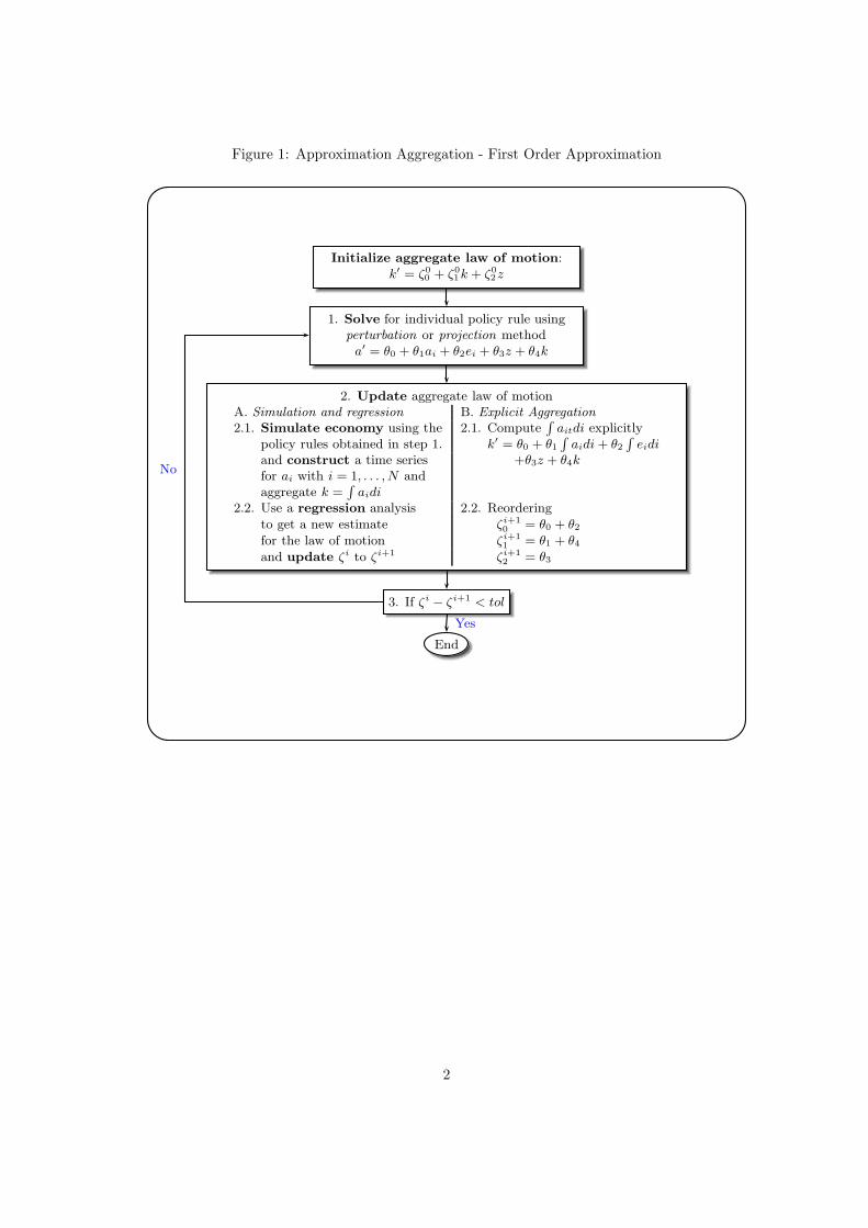
Figure 1: Approximation Aggregation - First Order Approximation
Initialize aggregate law of motion:k′ = ζ0
0 + ζ01k + ζ0
2z
1. Solve for individual policy rule usingperturbation or projection method
a′ = θ0 + θ1ai + θ2ei + θ3z + θ4k
2. Update aggregate law of motionA. Simulation and regression B. Explicit Aggregation
2.1. Simulate economy using the 2.1. ComputeR
aitdi explicitlypolicy rules obtained in step 1. k′ = θ0 + θ1
R
aidi + θ2
R
eidi
and construct a time series +θ3z + θ4k
for ai with i = 1, . . . , N andaggregate k =
R
aidi
2.2. Use a regression analysis 2.2. Reorderingto get a new estimate ζi+1
0 = θ0 + θ2
for the law of motion ζi+11 = θ1 + θ4
and update ζi to ζi+1 ζi+12 = θ3
3. If ζi− ζi+1 < tol
End
Yes
No
2
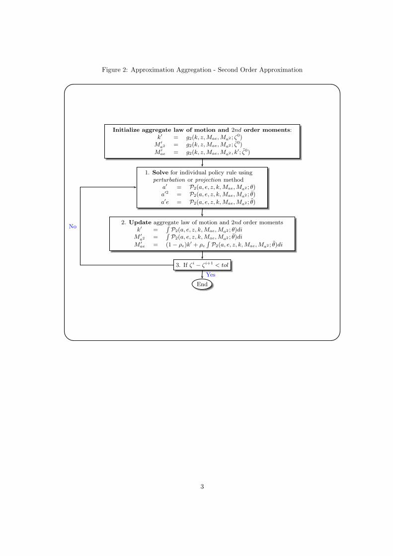
Figure 2: Approximation Aggregation - Second Order Approximation
Initialize aggregate law of motion and 2nd order moments:k′ = g2(k, z, Mae, Ma2 ; ζ0)
M ′
a2 = g2(k, z, Mae, Ma2 ; ζ0)
M ′
ae = g2(k, z, Mae, Ma2 , k′; ζ0)
1. Solve for individual policy rule usingperturbation or projection method
a′ = P2(a, e, z, k, Mae, Ma2 ; θ)a′2 = P2(a, e, z, k, Mae, Ma2 ; θ)
a′e = P2(a, e, z, k, Mae, Ma2 ; θ)
2. Update aggregate law of motion and 2nd order momentsk′ =
R
P2(a, e, z, k, Mae, Ma2 ; θ)di
M ′
a2 =R
P2(a, e, z, k, Mae, Ma2 ; θ)di
M ′
ae = (1 − ρe)k′ + ρe
R
P2(a, e, z, k, Mae, Ma2 ; θ)di
3. If ζi− ζi+1 < tol
End
Yes
No
3
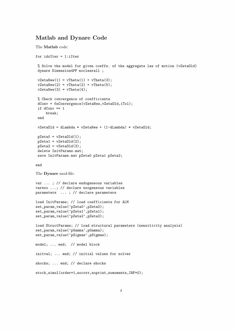
Matlab and Dynare Code
The Matlab code:
for idxIter = 1:iIter
% Solve the model for given coeffs. of the aggregate law of motion (vZetaOld)
dynare Dimension4PF noclearall ;
vZetaNew(1) = vTheta(1) + vTheta(3);
vZetaNew(2) = vTheta(2) + vTheta(5);
vZetaNew(3) = vTheta(4);
% Check convergence of coefficients
dConv = fnConvergence(vZetaNew,vZetaOld,iTol);
if dConv == 1
break;
end
vZetaOld = dLambda * vZetaNew + (1-dLambda) * vZetaOld;
pZeta0 = vZetaOld(1);
pZeta1 = vZetaOld(2);
pZeta2 = vZetaOld(3);
delete InitParams.mat;
save InitParams.mat pZeta0 pZeta1 pZeta2;
end
The Dynare mod-file:
var ... ; // declare endogeneous variables
varexo ...; // declare exogeneous variables
parameters ... ; // declare parameters
load InitParams; // load coefficients for ALM
set_param_value(’pZeta0’,pZeta0);
set_param_value(’pZeta1’,pZeta1);
set_param_value(’pZeta2’,pZeta2);
load StructParams; // load structural parameters (sensitivity analysis)
set_param_value(’pGamma’,pGamma);
set_param_value(’pSigmae’,pSigmae);
model; ... end; // model block
initval; ... end; // initial values for solver
shocks; ... end; // declare shocks
stoch_simul(order=1,nocorr,noprint,nomoments,IRF=0);
4

// Collecting parameters
mPolicy = [oo_.dr.ys’; oo_.dr.ghx’; oo_.dr.ghu’]; // read coefficients of policy
// functions
mPolA = mPolicy(:,2);
// Rearrange parameters
dTheta0 = mPolA(1)-mPolA(2)*mPolA(1)-mPolA(6)-mPolA(7)-mPolA(5)*mPolicy(1,5);
dTheta1 = mPolA(2);
dTheta2 = mPolA(6);
dTheta3 = mPolA(7);
dTheta4 = mPolA(5);
vTheta = [dTheta0 dTheta1 dTheta2 dTheta3 dTheta4];
5
Table 1: Convergence of the ALM coefficients during the updating process.
0 10 20 30 40 50 60 70 80−10
0
10
ζ 0
0 10 20 30 40 50 60 70 800
0.5
1
ζ 1
0 10 20 30 40 50 60 70 800
1
2
Iterations
ζ 2
(a) γ = 1.00
6
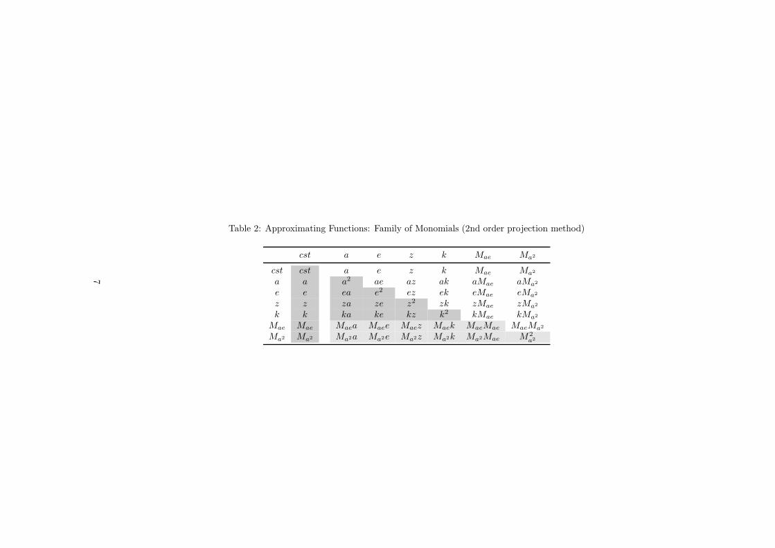
Table 2: Approximating Functions: Family of Monomials (2nd order projection method)
cst a e z k Mae Ma2
cst cst a e z k Mae Ma2
a a a2 ae az ak aMae aMa2
e e ea e2 ez ek eMae eMa2
z z za ze z2 zk zMae zMa2
k k ka ke kz k2 kMae kMa2
Mae Mae Maea Maee Maez Maek MaeMae MaeMa2
Ma2 M
a2 M
a2a M
a2e M
a2z M
a2k M
a2Mae M2
a2
7
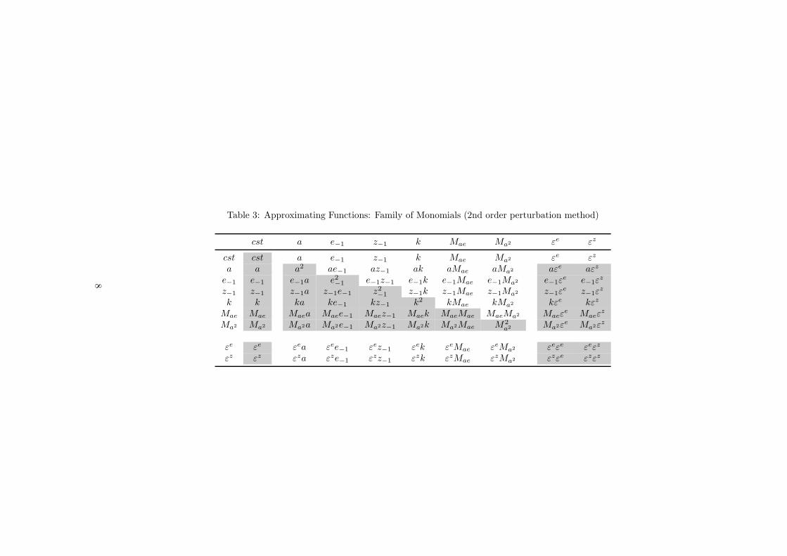
Table 3: Approximating Functions: Family of Monomials (2nd order perturbation method)
cst a e−1 z−1 k Mae Ma2 εe εz
cst cst a e−1 z−1 k Mae Ma2 εe εz
a a a2 ae−1 az−1 ak aMae aMa2 aεe aεz
e−1 e−1 e−1a e2−1 e−1z−1 e−1k e−1Mae e−1Ma
2 e−1εe e−1ε
z
z−1 z−1 z−1a z−1e−1 z2
−1z−1k z−1Mae z−1Ma
2 z−1εe z−1ε
z
k k ka ke−1 kz−1 k2 kMae kMa2 kεe kεz
Mae Mae Maea Maee−1 Maez−1 Maek MaeMae MaeMa2 Maeε
e Maeεz
Ma2 M
a2 M
a2a M
a2e−1 M
a2z−1 M
a2k M
a2Mae M2
a2 M
a2εe M
a2εz
εe εe εea εee−1 εez−1 εek εeMae εeMa2 εeεe εeεz
εz εz εza εze−1 εzz−1 εzk εzMae εzMa2 εzεe εzεz
8
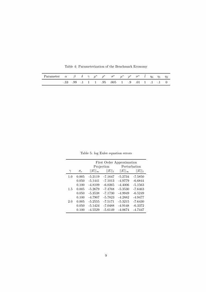
Table 4: Parameterization of the Benchmark Economy
Parameter α β δ γ µe ρe σe µz ρz σz l η0 η1 η2
.33 .99 .1 1 1 .95 .005 1 .9 .01 1 .1 .1 0
Table 5: log Euler equation errors
First Order ApproximationProjection Perturbation
γ σe ||E||∞ ||E||1 ||E||∞ ||E||1
1.0 0.005 -5.2119 -7.1647 -5.2734 -7.58500.050 -5.1441 -7.1013 -4.9779 -6.68440.100 -4.8109 -6.0265 -4.4006 -5.1563
1.5 0.005 -5.2679 -7.4768 -5.3530 -7.64630.050 -5.3538 -7.1730 -4.9949 -6.52490.100 -4.7907 -5.7823 -4.2882 -4.9477
2.0 0.005 -5.2555 -7.5171 -5.3215 -7.64300.050 -5.1424 -7.0488 -4.9148 -6.33720.100 -4.5529 -5.6149 -4.0674 -4.7447
9
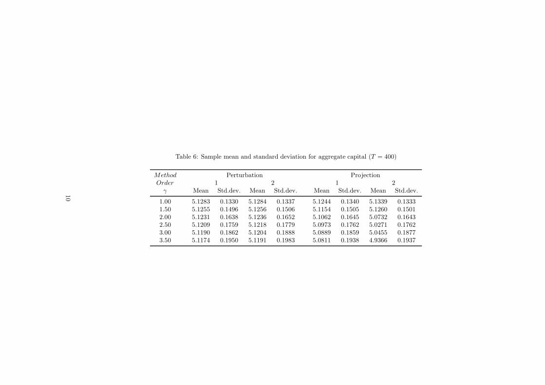
Table 6: Sample mean and standard deviation for aggregate capital (T = 400)
Method Perturbation ProjectionOrder 1 2 1 2
γ Mean Std.dev. Mean Std.dev. Mean Std.dev. Mean Std.dev.
1.00 5.1283 0.1330 5.1284 0.1337 5.1244 0.1340 5.1339 0.13331.50 5.1255 0.1496 5.1256 0.1506 5.1154 0.1505 5.1260 0.15012.00 5.1231 0.1638 5.1236 0.1652 5.1062 0.1645 5.0732 0.16432.50 5.1209 0.1759 5.1218 0.1779 5.0973 0.1762 5.0271 0.17623.00 5.1190 0.1862 5.1204 0.1888 5.0889 0.1859 5.0455 0.18773.50 5.1174 0.1950 5.1191 0.1983 5.0811 0.1938 4.9366 0.1937
10
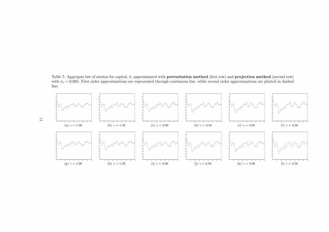
Table 7: Aggregate law of motion for capital, k, approximated with perturbation method (first row) and projection method (second row)with σe = 0.005. First order approximations are represented through continuous line, while second order approximations are plotted in dashedline.
50 100 150 200 250 300 350 4004
4.2
4.4
4.6
4.8
5
5.2
5.4
5.6
5.8
6
k
(a) γ = 1.00
50 100 150 200 250 300 350 4004
4.2
4.4
4.6
4.8
5
5.2
5.4
5.6
5.8
6
k
(b) γ = 1.50
50 100 150 200 250 300 350 4004
4.2
4.4
4.6
4.8
5
5.2
5.4
5.6
5.8
6
k
(c) γ = 2.00
50 100 150 200 250 300 350 4004
4.2
4.4
4.6
4.8
5
5.2
5.4
5.6
5.8
6
k
(d) γ = 2.50
50 100 150 200 250 300 350 4004
4.2
4.4
4.6
4.8
5
5.2
5.4
5.6
5.8
6
k
(e) γ = 3.00
50 100 150 200 250 300 350 4004
4.2
4.4
4.6
4.8
5
5.2
5.4
5.6
5.8
6
k
(f) γ = 3.50
50 100 150 200 250 300 350 4004
4.2
4.4
4.6
4.8
5
5.2
5.4
5.6
5.8
6
k
(g) γ = 1.00
50 100 150 200 250 300 350 4004
4.2
4.4
4.6
4.8
5
5.2
5.4
5.6
5.8
6
k
(h) γ = 1.50
50 100 150 200 250 300 350 4004
4.2
4.4
4.6
4.8
5
5.2
5.4
5.6
5.8
6
k
(i) γ = 2.00
50 100 150 200 250 300 350 4004
4.2
4.4
4.6
4.8
5
5.2
5.4
5.6
5.8
6
k
(j) γ = 2.50
50 100 150 200 250 300 350 4004
4.2
4.4
4.6
4.8
5
5.2
5.4
5.6
5.8
6
k
(k) γ = 3.00
50 100 150 200 250 300 350 4004
4.2
4.4
4.6
4.8
5
5.2
5.4
5.6
5.8
6
k
(l) γ = 3.50
11
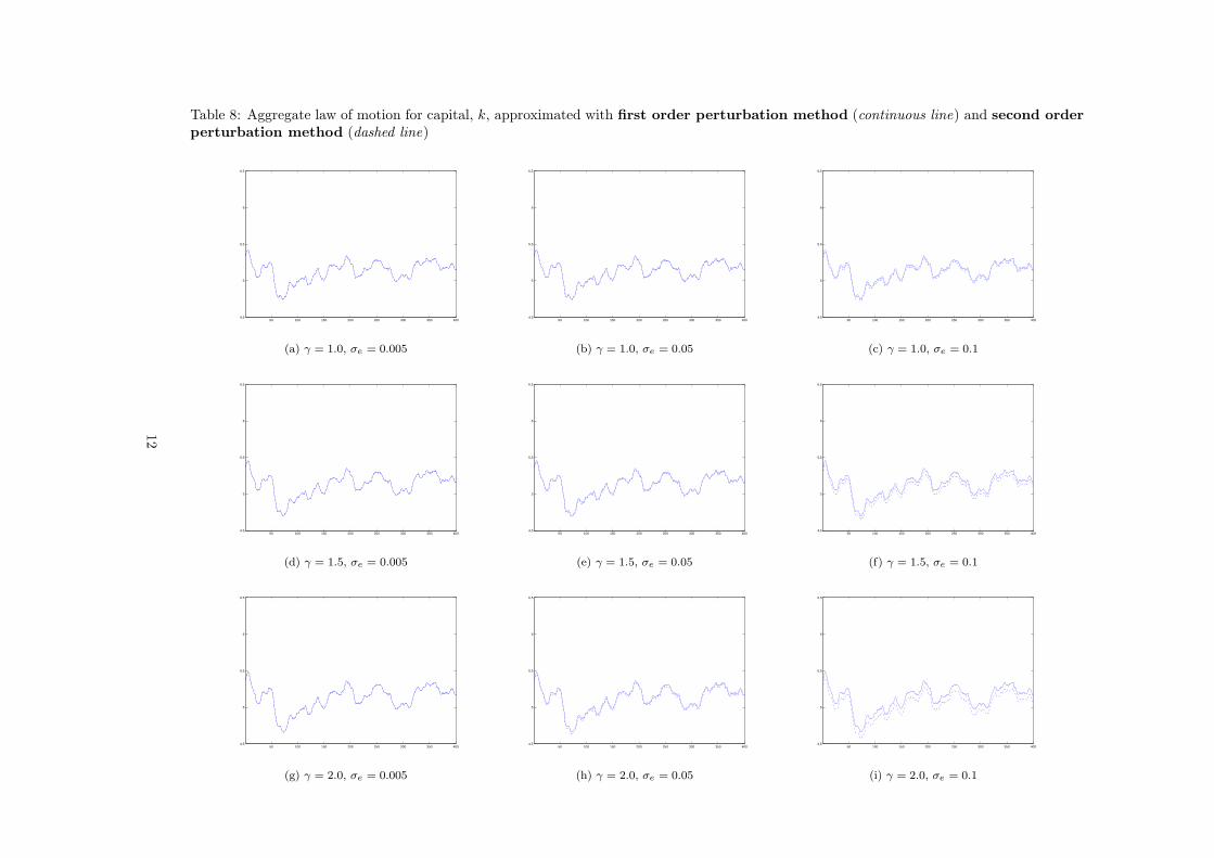
Table 8: Aggregate law of motion for capital, k, approximated with first order perturbation method (continuous line) and second order
perturbation method (dashed line)
50 100 150 200 250 300 350 4004.5
5
5.5
6
6.5
(a) γ = 1.0, σe = 0.005
50 100 150 200 250 300 350 4004.5
5
5.5
6
6.5
(b) γ = 1.0, σe = 0.05
50 100 150 200 250 300 350 4004.5
5
5.5
6
6.5
(c) γ = 1.0, σe = 0.1
50 100 150 200 250 300 350 4004.5
5
5.5
6
6.5
(d) γ = 1.5, σe = 0.005
50 100 150 200 250 300 350 4004.5
5
5.5
6
6.5
(e) γ = 1.5, σe = 0.05
50 100 150 200 250 300 350 4004.5
5
5.5
6
6.5
(f) γ = 1.5, σe = 0.1
50 100 150 200 250 300 350 4004.5
5
5.5
6
6.5
(g) γ = 2.0, σe = 0.005
50 100 150 200 250 300 350 4004.5
5
5.5
6
6.5
(h) γ = 2.0, σe = 0.05
50 100 150 200 250 300 350 4004.5
5
5.5
6
6.5
(i) γ = 2.0, σe = 0.1
12

Table 9: Results from First Order Approximation for γ = 1.0
Method for ALM Individual Policy Function Coefficients for the ALMθ0 θ1 θ2 θ3 θ4 ζ0 ζ1 ζ2
γ σe const a e z k const k z
1.0 0.005 Simulation Perturbation -0.67965 0.91636 0.37787 1.03880 -0.05953 -0.30165 0.85681 1.03873Projection -0.69286 0.91831 0.38486 1.04203 -0.06096 -0.30813 0.85735 1.04214
Xpa Perturbation -0.67961 0.91636 0.37787 1.03877 -0.05953 -0.30175 0.85683 1.03878Projection -0.69772 0.91869 0.38446 1.04509 -0.06091 -0.31062 0.85763 1.04315
0.05 Simulation Perturbation -0.67981 0.91636 0.37785 1.03914 -0.05956 -0.30086 0.85690 1.03746Projection -0.69204 0.91879 0.37657 1.05128 -0.06042 -0.31710 0.85860 1.05165
Xpa Perturbation -0.67961 0.91636 0.37787 1.03877 -0.05953 -0.30175 0.85683 1.03878Projection -0.69612 0.91897 0.37788 1.05298 -0.06040 -0.31850 0.85868 1.05269
0.1 Simulation Perturbation -0.67947 0.91636 0.37784 1.03965 -0.05973 -0.30001 0.85740 1.03401Projection -0.68543 0.92041 0.34434 1.08375 -0.05843 -0.34011 0.86216 1.08183
Xpa Perturbation -0.67961 0.91636 0.37787 1.03877 -0.05953 -0.30175 0.85683 1.03878Projection -0.68900 0.92054 0.34559 1.08491 -0.05836 -0.34479 0.86245 1.08491
13

Table 10: Results from First Order Approximation for γ = 1.5
Method for ALM Individual Policy Function Coefficients for the ALMθ0 θ1 θ2 θ3 θ4 ζ0 ζ1 ζ2
γ σe const a e z k const k z
1.5 0.005 Simulation Perturbation -0.81453 0.92867 0.41797 1.01232 -0.04828 -0.39642 0.88037 1.01224Projection -0.82294 0.93028 0.42339 1.01331 -0.04969 -0.39961 0.88059 1.01334
Xpa Perturbation -0.81449 0.92867 0.41797 1.01229 -0.04829 -0.39652 0.88038 1.01230Projection -0.81655 0.93019 0.42395 1.00935 -0.05019 -0.40450 0.88102 1.01602
0.05 Simulation Perturbation -0.81464 0.92867 0.41795 1.01265 -0.04832 -0.39544 0.88048 1.01066Projection -0.82802 0.93121 0.41417 1.02880 -0.04897 -0.41170 0.88229 1.02634
Xpa Perturbation -0.81449 0.92867 0.41797 1.01229 -0.04829 -0.39652 0.88038 1.01230Projection -0.84207 0.93202 0.41792 1.03330 -0.04865 -0.41798 0.88267 1.03070
0.1 Simulation Perturbation -0.81422 0.92867 0.41793 1.01310 -0.04849 -0.39422 0.88103 1.00662Projection -0.83385 0.93494 0.37473 1.08155 -0.04673 -0.46210 0.88960 1.07679
Xpa Perturbation -0.81449 0.92867 0.41797 1.01229 -0.04829 -0.39652 0.88038 1.01230Projection -0.82472 0.93437 0.37466 1.07504 -0.04675 -0.46713 0.88910 1.08486
14
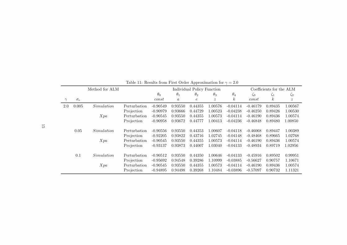
Table 11: Results from First Order Approximation for γ = 2.0
Method for ALM Individual Policy Function Coefficients for the ALMθ0 θ1 θ2 θ3 θ4 ζ0 ζ1 ζ2
γ σe const a e z k const k z
2.0 0.005 Simulation Perturbation -0.90549 0.93550 0.44355 1.00576 -0.04114 -0.46179 0.89435 1.00567Projection -0.90979 0.93666 0.44729 1.00523 -0.04238 -0.46250 0.89426 1.00530
Xpa Perturbation -0.90545 0.93550 0.44355 1.00573 -0.04114 -0.46190 0.89436 1.00574Projection -0.90958 0.93672 0.44777 1.00413 -0.04236 -0.46848 0.89480 1.00850
0.05 Simulation Perturbation -0.90556 0.93550 0.44353 1.00607 -0.04118 -0.46068 0.89447 1.00389Projection -0.92205 0.93822 0.43716 1.02745 -0.04148 -0.48468 0.89665 1.02768
Xpa Perturbation -0.90545 0.93550 0.44355 1.00573 -0.04114 -0.46190 0.89436 1.00574Projection -0.93137 0.93873 0.44007 1.03040 -0.04133 -0.48934 0.89719 1.02956
0.1 Simulation Perturbation -0.90512 0.93550 0.44350 1.00646 -0.04133 -0.45916 0.89502 0.99951Projection -0.95692 0.94548 0.39286 1.10999 -0.03885 -0.56627 0.90757 1.10671
Xpa Perturbation -0.90545 0.93550 0.44355 1.00573 -0.04114 -0.46190 0.89436 1.00574Projection -0.94895 0.94498 0.39268 1.10484 -0.03896 -0.57097 0.90732 1.11321
15
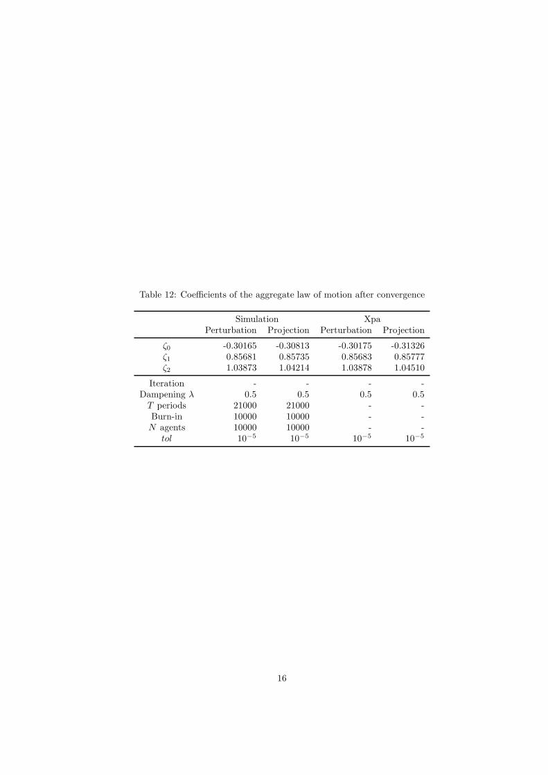
Table 12: Coefficients of the aggregate law of motion after convergence
Simulation XpaPerturbation Projection Perturbation Projection
ζ0 -0.30165 -0.30813 -0.30175 -0.31326ζ1 0.85681 0.85735 0.85683 0.85777ζ2 1.03873 1.04214 1.03878 1.04510
Iteration - - - -Dampening λ 0.5 0.5 0.5 0.5
T periods 21000 21000 - -Burn-in 10000 10000 - -N agents 10000 10000 - -
tol 10−5 10−5 10−5 10−5
16