Embed Size (px)
Citation preview
Motivation Discrete-Time Finite-State Stochastic Games Nonlinear Systems of Equations Extensions
Solving Dynamic Games with Newton’s Method
Karl Schmedders
University of Zurich and Swiss Finance Institute
Economic Applications of Modern Numerical Methods
Becker Friedman Institute, University of Chicago
Rosenwald Hall, Room 301 – November 1, 2013
Professor Kenneth L. Judd

Motivation Discrete-Time Finite-State Stochastic Games Nonlinear Systems of Equations Extensions
Discrete-Time Finite-State Stochastic Games
Central tool in analysis of strategic interactions amongforward-looking players in dynamic environments
Example: The Ericson & Pakes (1995) model of dynamiccompetition in an oligopolistic industry
Little analytical tractability
Most popular tool in the analysis: The Pakes & McGuire (1994)algorithm to solve numerically for an MPE (and variantsthereof)
Motivation Discrete-Time Finite-State Stochastic Games Nonlinear Systems of Equations Extensions
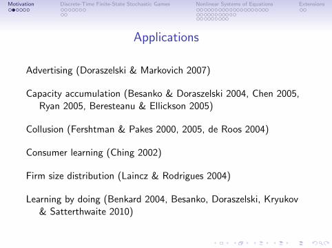
Applications
Advertising (Doraszelski & Markovich 2007)
Capacity accumulation (Besanko & Doraszelski 2004, Chen 2005,Ryan 2005, Beresteanu & Ellickson 2005)
Collusion (Fershtman & Pakes 2000, 2005, de Roos 2004)
Consumer learning (Ching 2002)
Firm size distribution (Laincz & Rodrigues 2004)
Learning by doing (Benkard 2004, Besanko, Doraszelski, Kryukov& Satterthwaite 2010)
Motivation Discrete-Time Finite-State Stochastic Games Nonlinear Systems of Equations Extensions
Applications cont’d
Mergers (Berry & Pakes 1993, Gowrisankaran 1999)
Network externalities (Jenkins, Liu, Matzkin & McFadden 2004,Markovich 2004, Markovich & Moenius 2007)
Productivity growth (Laincz 2005)
R&D (Gowrisankaran & Town 1997, Auerswald 2001, Song 2002,Judd et al. 2012)
Technology adoption (Schivardi & Schneider 2005)
International trade (Erdem & Tybout 2003)
Finance (Goettler, Parlour & Rajan 2004, Kadyrzhanova 2005).
Motivation Discrete-Time Finite-State Stochastic Games Nonlinear Systems of Equations Extensions
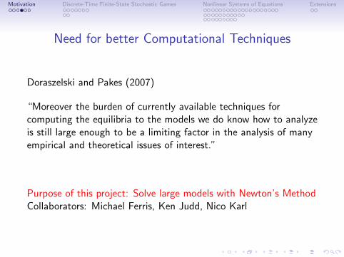
Need for better Computational Techniques
Doraszelski and Pakes (2007)
“Moreover the burden of currently available techniques forcomputing the equilibria to the models we do know how to analyzeis still large enough to be a limiting factor in the analysis of manyempirical and theoretical issues of interest.”
Purpose of this project: Solve large models with Newton’s MethodCollaborators: Michael Ferris, Ken Judd, Nico Karl
Motivation Discrete-Time Finite-State Stochastic Games Nonlinear Systems of Equations Extensions
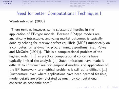
Need for better Computational Techniques II
Weintraub et al. (2008)
“There remain, however, some substantial hurdles in theapplication of EP-type models. Because EP-type models areanalytically intractable, analyzing market outcomes is typicallydone by solving for Markov perfect equilibria (MPE) numerically ona computer, using dynamic programming algorithms (e.g., Pakesand McGuire (1994)). This is a computational problem of thehighest order. [...] in practice computational concerns havetypically limited the analysis [...] Such limitations have made itdifficult to construct realistic empirical models, and application ofthe EP framework to empirical problems is still quite difficult [...]Furthermore, even where applications have been deemed feasible,model details are often dictated as much by computationalconcerns as economic ones.”
Motivation Discrete-Time Finite-State Stochastic Games Nonlinear Systems of Equations Extensions
Outline
MotivationBackground
Discrete-Time Finite-State Stochastic GamesCournot Duopoly GameMarkov Perfect Equilibrium
Nonlinear Systems of EquationsSolution MethodsNewton’s MethodSolving Large Games in PATH
ExtensionsNext Steps
Motivation Discrete-Time Finite-State Stochastic Games Nonlinear Systems of Equations Extensions
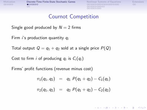
Cournot Competition
Single good produced by N = 2 firms
Firm i ’s production quantity qi
Total output Q = q1 + q2 sold at a single price P(Q)
Cost to firm i of producing qi is Ci (qi )
Firms’ profit functions (revenue minus cost)
π1(q1, q2) = q1 P(q1 + q2)− C1(q1)
π2(q1, q2) = q2 P(q1 + q2)− C2(q2)
Motivation Discrete-Time Finite-State Stochastic Games Nonlinear Systems of Equations Extensions
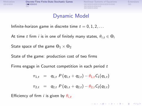
Dynamic Model
Infinite-horizon game in discrete time t = 0, 1, 2, . . .
At time t firm i is in one of finitely many states, θi ,t ∈ Θi
State space of the game Θ1 ×Θ2
State of the game: production cost of two firms
Firms engage in Cournot competition in each period t
π1,t = q1,t P (q1,t + q2,t)− θ1,tC1(q1,t)
π2,t = q2,t P (q1,t + q2,t)− θ2,tC2(q2,t)
Efficiency of firm i is given by θi ,t

Motivation Discrete-Time Finite-State Stochastic Games Nonlinear Systems of Equations Extensions
Learning and Investment
Firms’ states can change over time
Stochastic transition to state in next period depends onthree forces
Learning: current output may lead to lower production cost
Investment: firms can also make investment expenditures toreduce cost
Depreciation: shock to efficiency may increase cost
Motivation Discrete-Time Finite-State Stochastic Games Nonlinear Systems of Equations Extensions
Dynamic Setting
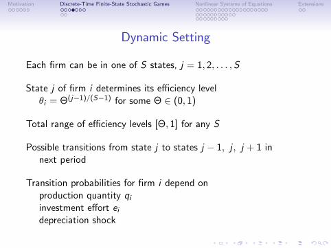
Each firm can be in one of S states, j = 1, 2, . . . ,S
State j of firm i determines its efficiency levelθi = Θ(j−1)/(S−1) for some Θ ∈ (0, 1)
Total range of efficiency levels [Θ, 1] for any S
Possible transitions from state j to states j − 1, j , j + 1 innext period
Transition probabilities for firm i depend onproduction quantity qiinvestment effort eidepreciation shock
Motivation Discrete-Time Finite-State Stochastic Games Nonlinear Systems of Equations Extensions
Transition Probabilities
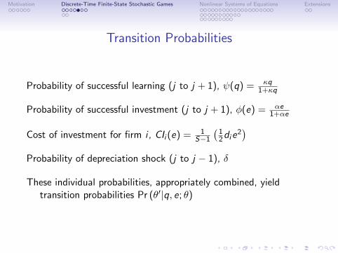
Probability of successful learning (j to j + 1), ψ(q) = κq1+κq
Probability of successful investment (j to j + 1), φ(e) = αe1+αe
Cost of investment for firm i , CIi (e) = 1S−1
(12die
2)
Probability of depreciation shock (j to j − 1), δ
These individual probabilities, appropriately combined, yieldtransition probabilities Pr (θ′|q, e; θ)
Motivation Discrete-Time Finite-State Stochastic Games Nonlinear Systems of Equations Extensions
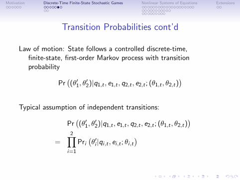
Transition Probabilities cont’d
Law of motion: State follows a controlled discrete-time,finite-state, first-order Markov process with transitionprobability
Pr((θ′1, θ
′2)|q1,t , e1,t , q2,t , e2,t ; (θ1,t , θ2,t)
)Typical assumption of independent transitions:
Pr((θ′1, θ
′2)|q1,t , e1,t , q2,t , e2,t ; (θ1,t , θ2,t)
)=
2∏i=1
Pri(θ′i |qi ,t , ei ,t ; θi ,t
)

Motivation Discrete-Time Finite-State Stochastic Games Nonlinear Systems of Equations Extensions
Objective Function
Notation: actions ut = (q1,t , e1,t , q2,t , e2,t), ui ,t = (qi ,t , ei ,t)states θt = (θ1,t , θ2,t)
Firm i receives total payoff Πi (ut ; θt) in period t fromCournot competition and investment
Objective is to maximize the expected NPV of future cash flows
E
{ ∞∑t=0
βtΠi (ut ; θt)
}
with discount factor β ∈ (0, 1)
Motivation Discrete-Time Finite-State Stochastic Games Nonlinear Systems of Equations Extensions
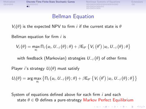
Bellman Equation
Vi (θ) is the expected NPV to firm i if the current state is θ
Bellman equation for firm i is
Vi (θ) = maxui
Πi (ui ,U−i (θ) ; θ) + βEθ′{Vi
(θ′)|ui ,U−i (θ) ; θ
}with feedback (Markovian) strategies U−i (θ) of other firms
Player i ’s strategy Ui (θ) must satisfy
Ui (θ) = arg maxui
{Πi (ui ,U−i (θ) ; θ) + βEθ′
{Vi
(θ′)|ui ,U−i (θ) ; θ
}}System of equations defined above for each firm i and each
state θ ∈ Θ defines a pure-strategy Markov Perfect Equilibrium
Motivation Discrete-Time Finite-State Stochastic Games Nonlinear Systems of Equations Extensions
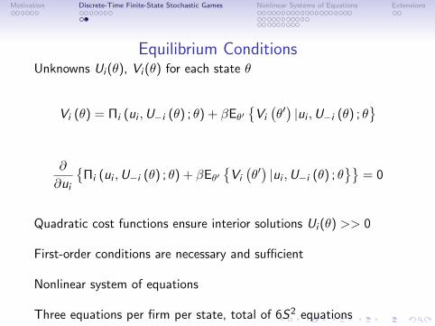
Equilibrium ConditionsUnknowns Ui (θ), Vi (θ) for each state θ
Vi (θ) = Πi (ui ,U−i (θ) ; θ) + βEθ′{Vi
(θ′)|ui ,U−i (θ) ; θ
}
∂
∂ui
{Πi (ui ,U−i (θ) ; θ) + βEθ′
{Vi
(θ′)|ui ,U−i (θ) ; θ
}}= 0
Quadratic cost functions ensure interior solutions Ui (θ) >> 0
First-order conditions are necessary and sufficient
Nonlinear system of equations
Three equations per firm per state, total of 6S2 equations
Motivation Discrete-Time Finite-State Stochastic Games Nonlinear Systems of Equations Extensions
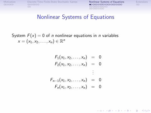
Nonlinear Systems of Equations
System F (x) = 0 of n nonlinear equations in n variablesx = (x1, x2, . . . , xn) ∈ Rn
F1(x1, x2, . . . , xn) = 0
F2(x1, x2, . . . , xn) = 0...
Fn−1(x1, x2, . . . , xn) = 0
Fn(x1, x2, . . . , xn) = 0
Motivation Discrete-Time Finite-State Stochastic Games Nonlinear Systems of Equations Extensions
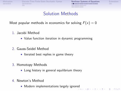
Solution Methods
Most popular methods in economics for solving F (x) = 0
1. Jacobi Method
• Value function iteration in dynamic programming
2. Gauss-Seidel Method
• Iterated best replies in game theory
3. Homotopy Methods
• Long history in general equilibrium theory
4. Newton’s Method
• Modern implementations largely ignored
Motivation Discrete-Time Finite-State Stochastic Games Nonlinear Systems of Equations Extensions
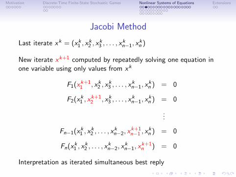
Jacobi Method
Last iterate xk = (xk1 , xk2 , x
k3 , . . . , x
kn−1, x
kn )
New iterate xk+1 computed by repeatedly solving one equation inone variable using only values from xk
F1(xk+11 , xk2 , x
k3 , . . . , x
kn−1, x
kn ) = 0
F2(xk1 , xk+12 , xk3 , . . . , x
kn−1, x
kn ) = 0
...
Fn−1(xk1 , xk2 , . . . , x
kn−2, x
k+1n−1 , x
kn ) = 0
Fn(xk1 , xk2 , . . . , x
kn−2, x
kn−1, x
k+1n ) = 0
Interpretation as iterated simultaneous best reply
Motivation Discrete-Time Finite-State Stochastic Games Nonlinear Systems of Equations Extensions
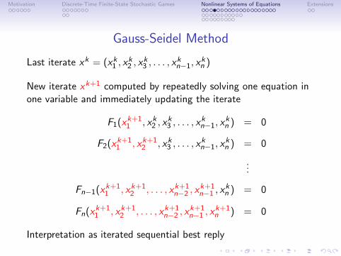
Gauss-Seidel Method
Last iterate xk = (xk1 , xk2 , x
k3 , . . . , x
kn−1, x
kn )
New iterate xk+1 computed by repeatedly solving one equation inone variable and immediately updating the iterate
F1(xk+11 , xk2 , x
k3 , . . . , x
kn−1, x
kn ) = 0
F2(xk+11 , xk+1
2 , xk3 , . . . , xkn−1, x
kn ) = 0
...
Fn−1(xk+11 , xk+1
2 , . . . , xk+1n−2 , x
k+1n−1 , x
kn ) = 0
Fn(xk+11 , xk+1
2 , . . . , xk+1n−2 , x
k+1n−1 , x
k+1n ) = 0
Interpretation as iterated sequential best reply
Motivation Discrete-Time Finite-State Stochastic Games Nonlinear Systems of Equations Extensions
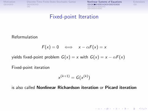
Fixed-point Iteration
Reformulation
F (x) = 0 ⇐⇒ x − αF (x) = x
yields fixed-point problem G (x) = x with G (x) = x − αF (x)
Fixed-point iteration
x (k+1) = G (x (k))
is also called Nonlinear Richardson iteration or Picard iteration
Motivation Discrete-Time Finite-State Stochastic Games Nonlinear Systems of Equations Extensions
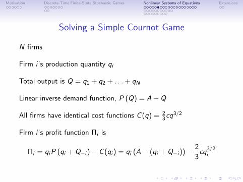
Solving a Simple Cournot Game
N firms
Firm i ’s production quantity qi
Total output is Q = q1 + q2 + . . .+ qN
Linear inverse demand function, P (Q) = A− Q
All firms have identical cost functions C (q) = 23cq
3/2
Firm i ’s profit function Πi is
Πi = qiP (qi + Q−i )− C (qi ) = qi (A− (qi + Q−i ))− 2
3cq
3/2i
Motivation Discrete-Time Finite-State Stochastic Games Nonlinear Systems of Equations Extensions
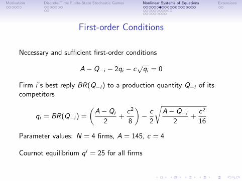
First-order Conditions
Necessary and sufficient first-order conditions
A− Q−i − 2qi − c√qi = 0
Firm i ’s best reply BR(Q−i ) to a production quantity Q−i of itscompetitors
qi = BR(Q−i ) =
(A− Qi
2+
c2
8
)− c
2
√A− Q−i
2+
c2
16
Parameter values: N = 4 firms, A = 145, c = 4
Cournot equilibrium qi = 25 for all firms
Motivation Discrete-Time Finite-State Stochastic Games Nonlinear Systems of Equations Extensions
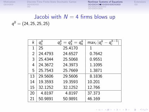
Jacobi with N = 4 firms blows upq0 = (24, 25, 25, 25)
k qk1 qk2 = qk3 = qk4 maxi |qki − qk−1i |1 25 25.4170 12 24.4793 24.6527 0.76423 25.4344 25.5068 0.95514 24.3672 24.3973 1.10955 25.7543 25.7669 1.3871
13 29.5606 29.5606 8.183614 19.3593 19.3593 10.20115 32.1252 32.1252 12.766
20 4.8197 4.8197 37.37321 50.9891 50.9891 46.169

Motivation Discrete-Time Finite-State Stochastic Games Nonlinear Systems of Equations Extensions
Solving the Cournot Game with Gauss-Seidel
q0 = (10, 10, 10, 10)
k qk1 qk2 qk3 qk4 maxi |qki − qk−1i |1 56.0294 32.1458 19.1583 11.9263 55.0292 29.9411 30.8742 25.9424 20.1446 26.0883 24.1839 26.9767 26.5433 23.8755 5.7571
10 25.0025 25.0016 24.9990 24.9987 5.6080 (−3)11 25.0003 25.0008 25.0001 24.9995 2.1669 (−3)12 24.9998 25.0003 25.0002 24.9999 5.8049 (−4)
16 25.0000 25.0000 25.0000 25.0000 1.1577 (−5)17 25.0000 25.0000 25.0000 25.0000 4.1482 (−6)18 25.0000 25.0000 25.0000 25.0000 1.1891 (−6)
Motivation Discrete-Time Finite-State Stochastic Games Nonlinear Systems of Equations Extensions
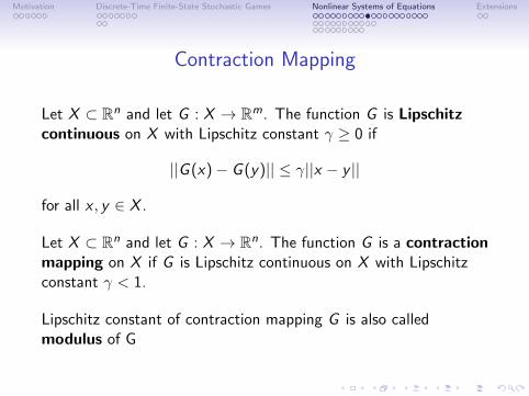
Contraction Mapping
Let X ⊂ Rn and let G : X → Rm. The function G is Lipschitzcontinuous on X with Lipschitz constant γ ≥ 0 if
||G (x)− G (y)|| ≤ γ||x − y ||
for all x , y ∈ X .
Let X ⊂ Rn and let G : X → Rn. The function G is a contractionmapping on X if G is Lipschitz continuous on X with Lipschitzconstant γ < 1.
Lipschitz constant of contraction mapping G is also calledmodulus of G
Motivation Discrete-Time Finite-State Stochastic Games Nonlinear Systems of Equations Extensions
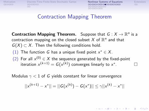
Contraction Mapping Theorem
Contraction Mapping Theorem. Suppose that G : X → Rn is acontraction mapping on the closed subset X of Rn and thatG (X ) ⊂ X . Then the following conditions hold.
(1) The function G has a unique fixed point x∗ ∈ X .
(2) For all x (0) ∈ X the sequence generated by the fixed-pointiteration x (k+1) = G (x (k)) converges linearly to x∗. �
Modulus γ < 1 of G yields constant for linear convergence
||x (k+1) − x∗|| = ||G (x (k))− G (x∗)|| ≤ γ||x (k) − x∗||

Motivation Discrete-Time Finite-State Stochastic Games Nonlinear Systems of Equations Extensions
Mode of Updating IteratesFixed-point iteration x (k+1) = G (x (k)) updates all components ofx simultaneously; Jacobi-mode of updating
x(k+1)i = Gi (x
(k)1 , x
(k)2 , . . . , x
(k)i−1, x
(k)i , x
(k)i+1, . . . , x
(k)n )
Gauss-Seidel mode of updating is also possible
x(k+1)i = Gi (x
(k+1)1 , x
(k+1)2 , . . . , x
(k+1)i−1 , x
(k)i , x
(k)i+1, . . . , x
(k)n )
Theorem. Suppose that G : X → Rn is a contraction mappingon the set X =
∏ni=1 Xi , where each Xi is a nonempty closed
subset of R, and that G (X ) ⊂ X . Then for all x (0) ∈ X thesequence generated by the fixed-point iteration x (k+1) = G (x (k))with a Gauss-Seidel mode of updating converges linearly to theunique fixed point x∗ of G . �
Motivation Discrete-Time Finite-State Stochastic Games Nonlinear Systems of Equations Extensions
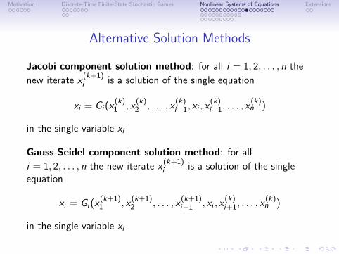
Alternative Solution Methods
Jacobi component solution method: for all i = 1, 2, . . . , n the
new iterate x(k+1)i is a solution of the single equation
xi = Gi (x(k)1 , x
(k)2 , . . . , x
(k)i−1, xi , x
(k)i+1, . . . , x
(k)n )
in the single variable xi
Gauss-Seidel component solution method: for all
i = 1, 2, . . . , n the new iterate x(k+1)i is a solution of the single
equation
xi = Gi (x(k+1)1 , x
(k+1)2 , . . . , x
(k+1)i−1 , xi , x
(k)i+1, . . . , x
(k)n )
in the single variable xi
Motivation Discrete-Time Finite-State Stochastic Games Nonlinear Systems of Equations Extensions
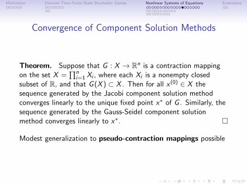
Convergence of Component Solution Methods
Theorem. Suppose that G : X → Rn is a contraction mappingon the set X =
∏ni=1 Xi , where each Xi is a nonempty closed
subset of R, and that G (X ) ⊂ X . Then for all x (0) ∈ X thesequence generated by the Jacobi component solution methodconverges linearly to the unique fixed point x∗ of G . Similarly, thesequence generated by the Gauss-Seidel component solutionmethod converges linearly to x∗. �
Modest generalization to pseudo-contraction mappings possible
Motivation Discrete-Time Finite-State Stochastic Games Nonlinear Systems of Equations Extensions
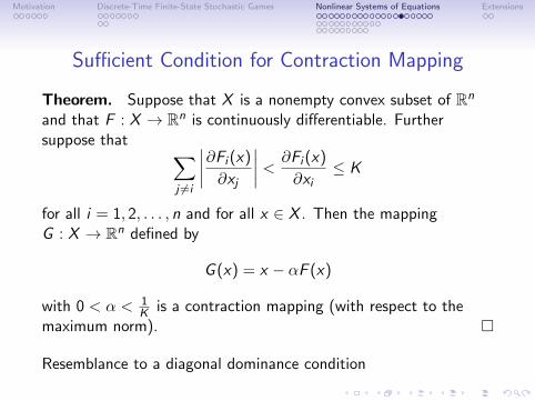
Sufficient Condition for Contraction Mapping
Theorem. Suppose that X is a nonempty convex subset of Rn
and that F : X → Rn is continuously differentiable. Furthersuppose that ∑
j 6=i
∣∣∣∣∂Fi (x)
∂xj
∣∣∣∣ < ∂Fi (x)
∂xi≤ K
for all i = 1, 2, . . . , n and for all x ∈ X . Then the mappingG : X → Rn defined by
G (x) = x − αF (x)
with 0 < α < 1K is a contraction mapping (with respect to the
maximum norm). �
Resemblance to a diagonal dominance condition
Motivation Discrete-Time Finite-State Stochastic Games Nonlinear Systems of Equations Extensions
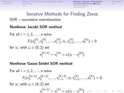
Iterative Methods for Finding ZerosSOR = successive overrelaxation
Nonlinear Jacobi SOR method
For all i = 1, 2, . . . , n solve
Fi (x(k)1 , x
(k)2 , . . . , x
(k)i−1, xi , x
(k)i+1, . . . , x
(k)n ) = 0
for xi ; with ω ∈ (0, 2) set
x(k+1)i = x
(k)i + ω(xi − x
(k)i )
Nonlinear Gauss-Seidel SOR method
For all i = 1, 2, . . . , n solve
Fi (x(k+1)1 , x
(k+1)2 , . . . , x
(k+1)i−1 , xi , x
(k)i+1, . . . , x
(k)n ) = 0
for xi ; with ω ∈ (0, 2) set
x(k+1)i = x
(k)i + ω(xi − x
(k)i )

Motivation Discrete-Time Finite-State Stochastic Games Nonlinear Systems of Equations Extensions
Global Convergence Theorem for Nonlinear SOR Methods
Theorem. Suppose the function F : Rn → Rn has the followingproperties.
(1) F is a continuous function from Rn onto Rn.
(2) F (x) ≤ F (y) implies x ≤ y for all x , y ∈ Rn.
(3) Fi : Rn → R is decreasing in xj for all j 6= i .
Then for ω ∈ (0, 1], any b ∈ Rn, and from any starting pointx0 ∈ Rn the sequences generated by the Jacobi SOR method andthe Gauss-Seidel SOR method, respectively, converge to the uniquesolution x∗ of F (x) = b. �
Motivation Discrete-Time Finite-State Stochastic Games Nonlinear Systems of Equations Extensions
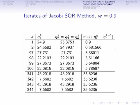
Iterates of Jacobi SOR Method, w = 0.9
k qk1 qk2 = qk3 = qk4 maxi |qki − qk−1i |1 24.9 25.3753 0.92 24.5682 24.7937 0.581566
97 27.731 27.731 5.3801198 22.2193 22.2193 5.5116699 27.8673 27.8673 5.64804
100 22.0815 22.0815 5.78587
341 43.2918 43.2918 35.6236342 7.6682 7.6682 35.6236343 43.2918 43.2918 35.6236344 7.6682 7.6682 35.6236
Motivation Discrete-Time Finite-State Stochastic Games Nonlinear Systems of Equations Extensions
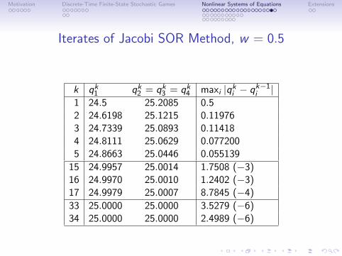
Iterates of Jacobi SOR Method, w = 0.5
k qk1 qk2 = qk3 = qk4 maxi |qki − qk−1i |1 24.5 25.2085 0.52 24.6198 25.1215 0.119763 24.7339 25.0893 0.114184 24.8111 25.0629 0.0772005 24.8663 25.0446 0.055139
15 24.9957 25.0014 1.7508 (−3)16 24.9970 25.0010 1.2402 (−3)17 24.9979 25.0007 8.7845 (−4)
33 25.0000 25.0000 3.5279 (−6)34 25.0000 25.0000 2.4989 (−6)
Motivation Discrete-Time Finite-State Stochastic Games Nonlinear Systems of Equations Extensions
Summary
Fixed-point iteration in all its variations (Jacobi mode orGauss-Seidel mode of updating, Jacobi or Gauss-Seidel componentsolution method) requires contraction property for convergence
Nonlinear Jacobi SOR or Gauss-Seidel SOR methods require strongmonotonicity properties for convergence
Conjecture: these sufficient conditions are rarely satisfied byeconomic models
Conclusion: do not be surprised if these methods do not work
Methods do have the advantage that they are easy to implement,which explains their popularity in economics
Motivation Discrete-Time Finite-State Stochastic Games Nonlinear Systems of Equations Extensions
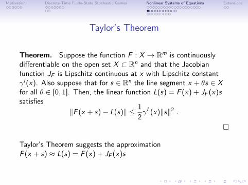
Taylor’s Theorem
Theorem. Suppose the function F : X → Rm is continuouslydifferentiable on the open set X ⊂ Rn and that the Jacobianfunction JF is Lipschitz continuous at x with Lipschitz constantγ l(x). Also suppose that for s ∈ Rn the line segment x + θs ∈ Xfor all θ ∈ [0, 1]. Then, the linear function L(s) = F (x) + JF (x)ssatisfies
‖F (x + s)− L(s)‖ ≤ 1
2γL(x)‖s‖2 .
�
Taylor’s Theorem suggests the approximationF (x + s) ≈ L(s) = F (x) + JF (x)s
Motivation Discrete-Time Finite-State Stochastic Games Nonlinear Systems of Equations Extensions
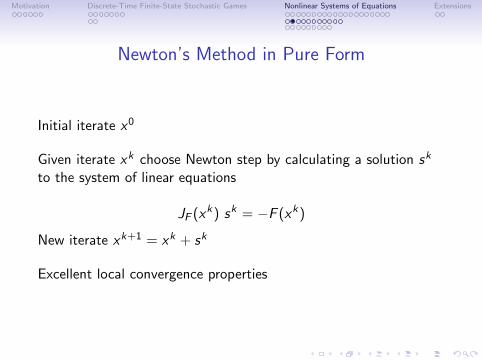
Newton’s Method in Pure Form
Initial iterate x0
Given iterate xk choose Newton step by calculating a solution sk
to the system of linear equations
JF (xk) sk = −F (xk)
New iterate xk+1 = xk + sk
Excellent local convergence properties
Motivation Discrete-Time Finite-State Stochastic Games Nonlinear Systems of Equations Extensions
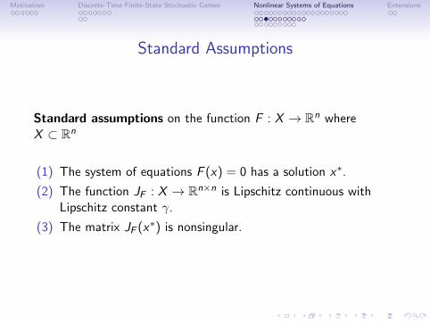
Standard Assumptions
Standard assumptions on the function F : X → Rn whereX ⊂ Rn
(1) The system of equations F (x) = 0 has a solution x∗.
(2) The function JF : X → Rn×n is Lipschitz continuous withLipschitz constant γ.
(3) The matrix JF (x∗) is nonsingular.
Motivation Discrete-Time Finite-State Stochastic Games Nonlinear Systems of Equations Extensions
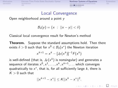
Local ConvergenceOpen neighborhood around a point y
Bδ(y) = {x : ||x − y || < δ}
Classical local convergence result for Newton’s method
Theorem. Suppose the standard assumptions hold. Then thereexists δ > 0 such that for x0 ∈ Bδ(x∗) the Newton iteration
xk+1 = xk − [JF (xk)]−1F (xk)
is well-defined (that is, JF (xk) is nonsingular) and generates asequence of iterates x0, x1, . . . , xk , xk+1, . . . which convergesquadratically to x∗, that is, for all sufficiently large k , there isK > 0 such that
||xk+1 − x∗|| ≤ K ||xk − x∗||2.
�
Motivation Discrete-Time Finite-State Stochastic Games Nonlinear Systems of Equations Extensions
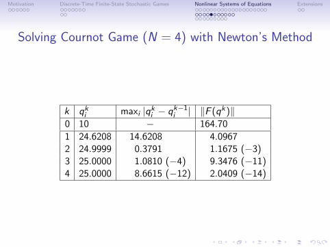
Solving Cournot Game (N = 4) with Newton’s Method
k qki maxi |qki − qk−1i | ‖F (qk)‖0 10 − 164.70
1 24.6208 14.6208 4.09672 24.9999 0.3791 1.1675 (−3)3 25.0000 1.0810 (−4) 9.3476 (−11)4 25.0000 8.6615 (−12) 2.0409 (−14)
Motivation Discrete-Time Finite-State Stochastic Games Nonlinear Systems of Equations Extensions
Shortcomings of Newton’s Method
If initial guess x0 is far from a solution Newton’s method maybehave erratically; for example, it may diverge or cycle
If JF (xk) is singular the Newton step may not be defined
It may be too expensive to compute the Newton step sk for largesystems of equations
The root x∗ may be degenerate (JF (x∗) is singular) andconvergence is very slow
Practical variants of Newton-like methods overcome most of theseissues
Motivation Discrete-Time Finite-State Stochastic Games Nonlinear Systems of Equations Extensions
Merit Function for Newton’s MethodGeneral idea: Obtain global convergence by combining the Newtonstep with line-search or trust-region methods from optimization
Merit function monitors progress towards root of F
Most widely used merit function is sum of squares
M(x) =1
2‖F (x)‖2 =
1
2
n∑i=1
F 2i (x)
Any root x∗ of F yields global minimum of M
Local minimizers with M(x) > 0 are not roots of F
∇M(x̃) = JF (x̃)>F (x̃) = 0
and so F (x̃) 6= 0 implies JF (x̃) is singular
Motivation Discrete-Time Finite-State Stochastic Games Nonlinear Systems of Equations Extensions
Line-Search Method
Newton stepJf (xk) sk = −F (xk)
yields a descent direction of M as long as F (xk) 6= 0(sk)>∇M(xk) =
(sk)>
JF (xk)>F (xk) = −‖F (xk)‖2 < 0
Given step length αk the new iterate is
xk+1 = xk + αksk
Motivation Discrete-Time Finite-State Stochastic Games Nonlinear Systems of Equations Extensions
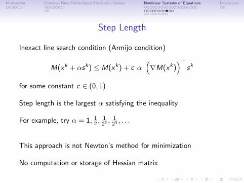
Step Length
Inexact line search condition (Armijo condition)
M(xk + αsk) ≤ M(xk) + c α(∇M(xk)
)>sk
for some constant c ∈ (0, 1)
Step length is the largest α satisfying the inequality
For example, try α = 1, 12 ,122, 123, . . .
This approach is not Newton’s method for minimization
No computation or storage of Hessian matrix
Motivation Discrete-Time Finite-State Stochastic Games Nonlinear Systems of Equations Extensions
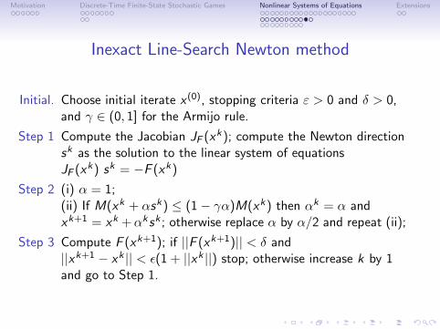
Inexact Line-Search Newton method
Initial. Choose initial iterate x (0), stopping criteria ε > 0 and δ > 0,and γ ∈ (0, 1] for the Armijo rule.
Step 1 Compute the Jacobian JF (xk); compute the Newton directionsk as the solution to the linear system of equationsJF (xk) sk = −F (xk)
Step 2 (i) α = 1;(ii) If M(xk + αsk) ≤ (1− γα)M(xk) then αk = α andxk+1 = xk +αksk ; otherwise replace α by α/2 and repeat (ii);
Step 3 Compute F (xk+1); if ||F (xk+1)|| < δ and||xk+1 − xk || < ε(1 + ||xk ||) stop; otherwise increase k by 1and go to Step 1.

Motivation Discrete-Time Finite-State Stochastic Games Nonlinear Systems of Equations Extensions
Global Convergence
Assumption. The function F is well defined and the Jacobian JFis Lipschitz continuous with Lipschitz constant γ in an openneighborhood of the level set L =
{x : ‖F (x)‖ ≤ ‖F (x0)‖
}for the
initial iterate x0. Moreover, ‖J−1F ‖ is bounded on L. �
Theorem. Suppose the assumption above holds. If the sequence{xk} generated by the inexact line search Newton method with theArmijo rule remains bounded then it converges to a root x∗ of F atwhich the standard assumptions hold, that is, full steps are takenfor k sufficiently large and the rate of convergence is quadratic. �
Motivation Discrete-Time Finite-State Stochastic Games Nonlinear Systems of Equations Extensions
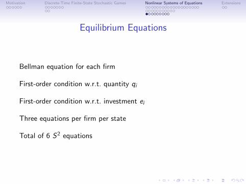
Equilibrium Equations
Bellman equation for each firm
First-order condition w.r.t. quantity qi
First-order condition w.r.t. investment ei
Three equations per firm per state
Total of 6 S2 equations
Motivation Discrete-Time Finite-State Stochastic Games Nonlinear Systems of Equations Extensions
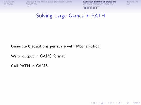
Solving Large Games in PATH
Generate 6 equations per state with Mathematica
Write output in GAMS format
Call PATH in GAMS
Motivation Discrete-Time Finite-State Stochastic Games Nonlinear Systems of Equations Extensions
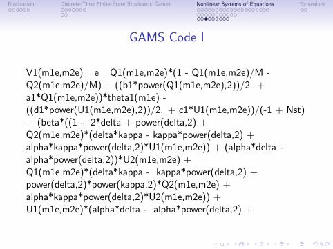
GAMS Code I
V1(m1e,m2e) =e= Q1(m1e,m2e)*(1 - Q1(m1e,m2e)/M -Q2(m1e,m2e)/M) - ((b1*power(Q1(m1e,m2e),2))/2. +a1*Q1(m1e,m2e))*theta1(m1e) -((d1*power(U1(m1e,m2e),2))/2. + c1*U1(m1e,m2e))/(-1 + Nst)+ (beta*((1 - 2*delta + power(delta,2) +Q2(m1e,m2e)*(delta*kappa - kappa*power(delta,2) +alpha*kappa*power(delta,2)*U1(m1e,m2e)) + (alpha*delta -alpha*power(delta,2))*U2(m1e,m2e) +Q1(m1e,m2e)*(delta*kappa - kappa*power(delta,2) +power(delta,2)*power(kappa,2)*Q2(m1e,m2e) +alpha*kappa*power(delta,2)*U2(m1e,m2e)) +U1(m1e,m2e)*(alpha*delta - alpha*power(delta,2) +
Motivation Discrete-Time Finite-State Stochastic Games Nonlinear Systems of Equations Extensions
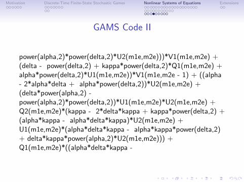
GAMS Code II
power(alpha,2)*power(delta,2)*U2(m1e,m2e)))*V1(m1e,m2e) +(delta - power(delta,2) + kappa*power(delta,2)*Q1(m1e,m2e) +alpha*power(delta,2)*U1(m1e,m2e))*V1(m1e,m2e - 1) + ((alpha- 2*alpha*delta + alpha*power(delta,2))*U2(m1e,m2e) +(delta*power(alpha,2) -power(alpha,2)*power(delta,2))*U1(m1e,m2e)*U2(m1e,m2e) +Q2(m1e,m2e)*(kappa - 2*delta*kappa + kappa*power(delta,2) +(alpha*kappa - alpha*delta*kappa)*U2(m1e,m2e) +U1(m1e,m2e)*(alpha*delta*kappa - alpha*kappa*power(delta,2)+ delta*kappa*power(alpha,2)*U2(m1e,m2e))) +Q1(m1e,m2e)*((alpha*delta*kappa -
Motivation Discrete-Time Finite-State Stochastic Games Nonlinear Systems of Equations Extensions
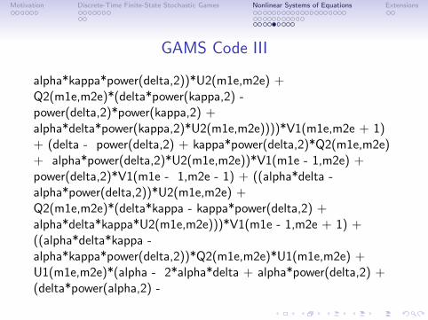
GAMS Code III
alpha*kappa*power(delta,2))*U2(m1e,m2e) +Q2(m1e,m2e)*(delta*power(kappa,2) -power(delta,2)*power(kappa,2) +alpha*delta*power(kappa,2)*U2(m1e,m2e))))*V1(m1e,m2e + 1)+ (delta - power(delta,2) + kappa*power(delta,2)*Q2(m1e,m2e)+ alpha*power(delta,2)*U2(m1e,m2e))*V1(m1e - 1,m2e) +power(delta,2)*V1(m1e - 1,m2e - 1) + ((alpha*delta -alpha*power(delta,2))*U2(m1e,m2e) +Q2(m1e,m2e)*(delta*kappa - kappa*power(delta,2) +alpha*delta*kappa*U2(m1e,m2e)))*V1(m1e - 1,m2e + 1) +((alpha*delta*kappa -alpha*kappa*power(delta,2))*Q2(m1e,m2e)*U1(m1e,m2e) +U1(m1e,m2e)*(alpha - 2*alpha*delta + alpha*power(delta,2) +(delta*power(alpha,2) -
Motivation Discrete-Time Finite-State Stochastic Games Nonlinear Systems of Equations Extensions
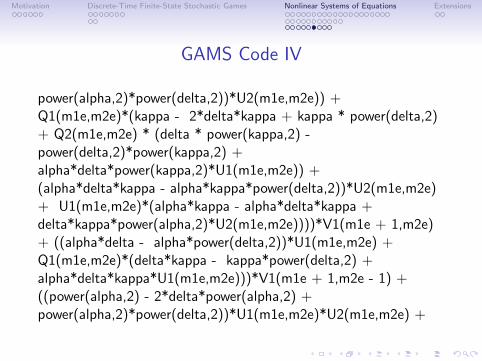
GAMS Code IV
power(alpha,2)*power(delta,2))*U2(m1e,m2e)) +Q1(m1e,m2e)*(kappa - 2*delta*kappa + kappa * power(delta,2)+ Q2(m1e,m2e) * (delta * power(kappa,2) -power(delta,2)*power(kappa,2) +alpha*delta*power(kappa,2)*U1(m1e,m2e)) +(alpha*delta*kappa - alpha*kappa*power(delta,2))*U2(m1e,m2e)+ U1(m1e,m2e)*(alpha*kappa - alpha*delta*kappa +delta*kappa*power(alpha,2)*U2(m1e,m2e))))*V1(m1e + 1,m2e)+ ((alpha*delta - alpha*power(delta,2))*U1(m1e,m2e) +Q1(m1e,m2e)*(delta*kappa - kappa*power(delta,2) +alpha*delta*kappa*U1(m1e,m2e)))*V1(m1e + 1,m2e - 1) +((power(alpha,2) - 2*delta*power(alpha,2) +power(alpha,2)*power(delta,2))*U1(m1e,m2e)*U2(m1e,m2e) +
Motivation Discrete-Time Finite-State Stochastic Games Nonlinear Systems of Equations Extensions
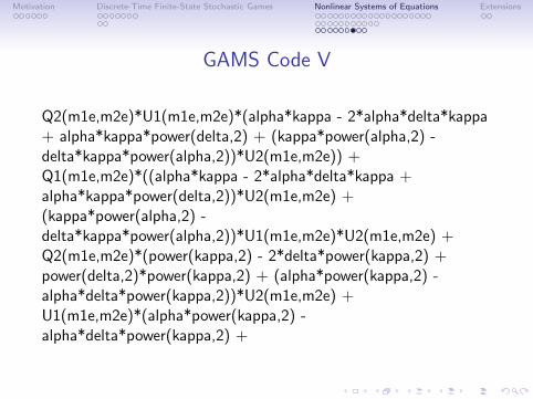
GAMS Code V
Q2(m1e,m2e)*U1(m1e,m2e)*(alpha*kappa - 2*alpha*delta*kappa+ alpha*kappa*power(delta,2) + (kappa*power(alpha,2) -delta*kappa*power(alpha,2))*U2(m1e,m2e)) +Q1(m1e,m2e)*((alpha*kappa - 2*alpha*delta*kappa +alpha*kappa*power(delta,2))*U2(m1e,m2e) +(kappa*power(alpha,2) -delta*kappa*power(alpha,2))*U1(m1e,m2e)*U2(m1e,m2e) +Q2(m1e,m2e)*(power(kappa,2) - 2*delta*power(kappa,2) +power(delta,2)*power(kappa,2) + (alpha*power(kappa,2) -alpha*delta*power(kappa,2))*U2(m1e,m2e) +U1(m1e,m2e)*(alpha*power(kappa,2) -alpha*delta*power(kappa,2) +
Motivation Discrete-Time Finite-State Stochastic Games Nonlinear Systems of Equations Extensions
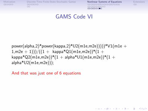
GAMS Code VI
power(alpha,2)*power(kappa,2)*U2(m1e,m2e)))))*V1(m1e +1,m2e + 1)))/((1 + kappa*Q1(m1e,m2e))*(1 +kappa*Q2(m1e,m2e))*(1 + alpha*U1(m1e,m2e))*(1 +alpha*U2(m1e,m2e)));
And that was just one of 6 equations

Motivation Discrete-Time Finite-State Stochastic Games Nonlinear Systems of Equations Extensions
Results
S Var rows non-zero dense(%) Steps RT (m:s)
20 2400 2568 31536 0.48 5 0 : 0350 15000 15408 195816 0.08 5 0 : 19100 60000 60808 781616 0.02 5 1 : 16200 240000 241608 3123216 0.01 5 5 : 12
Convergence for S = 200
Iteration Residual
0 1.56(+4)1 1.06(+1)2 1.343 2.04(−2)4 1.74(−5)5 2.97(−11)
Motivation Discrete-Time Finite-State Stochastic Games Nonlinear Systems of Equations Extensions
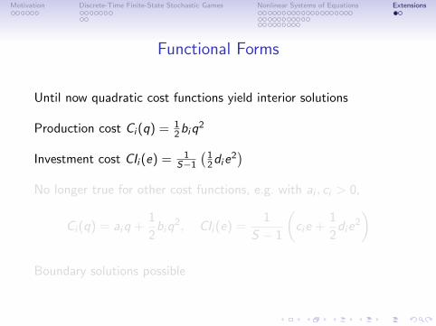
Functional Forms
Until now quadratic cost functions yield interior solutions
Production cost Ci (q) = 12biq
2
Investment cost CIi (e) = 1S−1
(12die
2)
No longer true for other cost functions, e.g. with ai , ci > 0,
Ci (q) = aiq +1
2biq
2, CIi (e) =1
S − 1
(cie +
1
2die
2
)
Boundary solutions possible
Motivation Discrete-Time Finite-State Stochastic Games Nonlinear Systems of Equations Extensions
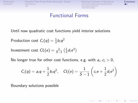
Functional Forms
Until now quadratic cost functions yield interior solutions
Production cost Ci (q) = 12biq
2
Investment cost CIi (e) = 1S−1
(12die
2)
No longer true for other cost functions, e.g. with ai , ci > 0,
Ci (q) = aiq +1
2biq
2, CIi (e) =1
S − 1
(cie +
1
2die
2
)
Boundary solutions possible
Motivation Discrete-Time Finite-State Stochastic Games Nonlinear Systems of Equations Extensions
Complementarity Problems
First-order conditions remain necessary and sufficientbut become nonlinear complementarity conditions
0 ≤ ui ⊥ −∂
∂ui
{Πi (ui ,U−i (θ) ; θ) + βEθ′
{Vi
(θ′)|ui ,U−i (θ) ; θ
}}≥ 0
Together with value function equations we obtain amixed complementarity problem
Initial results indicate that PATH solves MCPs almost as fast asnonlinear equations

![Solving games - Software Technologymarijn/publications/solving_games.pdf · In this paper we will focus predominantly on solved games - those games for ... solving games [10], van](https://img.pdfslide.us/doc/110x75/5ac8e6d87f8b9aa3298c80d1/solving-games-software-marijnpublicationssolvinggamespdfin-this-paper-we-will.jpg)