Solving a Class of PDEs by a Local Reproducing Kernel Method … · Method with An Adaptive Residual Subsampling Technique H. Raﬁeayan Zadeh1, ... and Russell (1990a); Huang, Ren,

Copyright © 2015 Tech Science Press CMES, vol.108, no.6, pp.375-396, 2015

Solving a Class of PDEs by a Local Reproducing KernelMethod with An Adaptive Residual Subsampling

Technique

H. Rafieayan Zadeh1, M. Mohammadi1,2 and E. Babolian1

Abstract: A local reproducing kernel method based on spatial trial space spannedby the Newton basis functions in the native Hilbert space of the reproducing kernelis proposed. It is a truly meshless approach which uses the local sub clusters of do-main nodes for approximation of the arbitrary field. It leads to a system of ordinarydifferential equations (ODEs) for the time-dependent partial differential equations(PDEs). An adaptive algorithm, so-called adaptive residual subsampling, is used toadjust nodes in order to remove oscillations which are caused by a sharp gradient.The method is applied for solving the Allen-Cahn and Burgers’ equations. The nu-merical results show that the proposed method is efficient, accurate and be able toremove oscillations caused by sharp gradient.

Keywords: Local reproducing kernel method, method of lines, Newton basisfunctions, adaptive residual subsampling algorithm.

1 Introduction

During last decades, meshless methods are considered by many researchers. Unliketraditional numerical methods in solving PDEs, meshless methods [Belytschko,Krongauz, Organ, Fleming, and Krysl (1996)] need no mesh generation. Tak-ing translates of kernels as trial functions in collocation methods, which are tru-ly meshless, leads to a highly successful method [C. Franke (1998); Huang, Ren,and Russell (1990a); Huang, Ren, and Russell (1990b)]. Implementation of thesemethods is easy and allow good accuracy at low computational cost. In addition,it was proven recently [Schaback (2015)] that symmetric collocation using kernelsis optimal along all linear PDE solvers using the same input data. There are plentyof papers which use kernel-based methods for solving various problems [Abbas-

1 Faculty of Mathematical Sciences and Computer, Kharazmi University, 50 Taleghani Ave., Tehran1561836314, Iran

2 Corresponding author

376 Copyright © 2015 Tech Science Press CMES, vol.108, no.6, pp.375-396, 2015

bandy, Azarnavid, and Alhuthali (2014); Atluri and Shen (2003); Dong, Alotaibi,Mohiuddine, and Atluri (2014); Elgohary, Dong, Junkins, and Atluri (2014); Hanand Atluri (2014); Hon and Schaback (2008); Mohammadi and Mokhtari (2014);Mohammadi and Mokhtari (2011); Mohammadi and Mokhtari (2013); Moham-madi, Mokhtari, and Panahipour (2013); Mohammadi, Mokhtari, and Panahipour(2014); Mohammadi, Mokhtari, and Schaback (2014); Mohammadi, Mokhtari, andIsfahani (2014); Mokhtari, Isfahani, and Mohammadi (2012)].

It is well known that representations of kernel-based approximants in terms of thestandard basis of translated kernels are notoriously unstable. A more useful basis,so-called Newton basis, is offered in [Muller and Schaback (2009)]. The Newtonbasis turns out to be orthonomal in the reproducing native Hilbert space, and it iscomplete, if infinitely many data locations are reasonably chosen. A timesavingcalculation of Newton basis arising from a pivoted Cholesky factorization has beenintroduced in [Pazouki and Schaback (2011)].

For the time-dependent PDEs, a spatial interpolation is applied by using expansionin terms of kernel functions. But since the coefficients are time-dependent, a sys-tem of ODEs is obtained. This is the well-known method of lines (MOL), and itturns out to be approximately useful in various cases. In this paper, we use ex-pansion in terms of the Newton basis functions (NBFs) for constructing the spatialinterpolation.

In global collocation methods, collocation matrix is made by considering the wholedomain, since the obtained matrix will be full. This limits the applicability of thosemethods to solve large scale problems. But local methods [Chen, Ganesh, Golberg,and Cheng (2002); Lee, Liu, and Fan (2003); Mai-Duy and Tran-Cong (2002)] useoverlapping sub-domains of the whole domain, thus a sparse matrix is obtained.A general idea behind the local reproducing kernel method is the use of the localsub clusters of domain nodes, named local influence domain, for approximation ofthe arbitrary field. With the selected influence domain, an approximation functionis introduced as a sum of weighted NBFs. Then the collocation approach is usedto determine weights. After the successful approximation function creation all theneeded differential operators can be constructed by applying an arbitrary operatoron the approximation function. The main advantage to using the local method isthat less computer storage and flops are needed.

The kernel functions are defined by using a set of points called centers or trialpoints. The centers can set anywhere of given domain independently, therefore,center points can be moved or added or removed in the domain and this is the baseof adaptive algorithms. Positions of the centers set influence on approximationquality and stability of the interpolation [Schaback (1995)], in addition, increasingnumber of centers causes large condition numeber of interpolation matrix. Adap-

Solving a Class of PDEs by a Local Reproducing Kernel Method 377

tive algorithms are often applied for problems containing rapid variations in thegiven domain. Different kinds of adaptive methods have been developed in theliterature, e.g. Greedy algorithm [Ling, Opfe, and Schaback (2006); Ling and Sch-aback (2009)], upwind technique [Lin and Atluri (2000); Lin and Atluri (2001)],r-adaptive mesh method (moving mesh strategy) [Huang, Ren, and Russell (1994)].Four kinds of center choosing algorithms with some algorithmic analysis are intro-duced in [Gong, Wei, Wang, Feng, and Wang (2010)]. In this paper, we use adaptiveresidual subsampling method [Driscoll and Heryudono (2007)], where nodes canbe added or removed based on interpolation residuals evaluated at a finer point set.In the adaptive residual subsampling algorithm, an interpolant has been computedfor the center set, the residual of the resulting approximation is sampled on a finernode set. Nodes from the finer set are added to or removed from the set of centersbased on the size of the residual of the interpolation at those points. The interpolantis then recomputed using the new center set for a new approximation.

In this study, we use a local reproducing kernel method based on spatial trial spacespanned by the NBFs accompanied with an adaptive residual subsampling tech-nique for the numerical solution of a class of PDEs including the Allen-Cahn andBurgers’ equations with different kinds of initial and boundary conditions. TheAllen-Cahn equation describes the motion of anti-phase boundaries in crystallinesolids. It has been widely used in material science applications. The Burgers’ equa-tion is the simplest nonlinear model equation for diffusive waves in fluid dynamics.The Burgers’ equation arises in many physical problems including one- dimension-al turbulence, sound waves in a viscous medium, shock waves in a viscous medium,waves in fluid filled viscous elastic tubes, and magneto-hydrodynamic waves in amedium with finite electrical conductivity. The Burgers’ equation is similar to theone dimensional Navier-Stokes equation without the stress term.

The rest of the paper is organized as follows. In section 2, the kernel-based tri-al functions and the NBFs are reviewed. The proposed local reproducing kernelmethod is given in section 3. The method is illustrated in section 4 by solving thenonlinear Allen-Cahn equation with mixed boundary conditions. In section 5, theadaptive residual subsampling algorithm is illustrated. Numerical experiments aregiven in section 6. The last section is devoted to a brief conclusion.

2 Kernel-based trial functions

Let Ω be a nonempty set. A function K : Ω×Ω→ R is called a kernel on Ω. LetK : Ω×Ω→ R be a symmetric positive definite kernel on Ω. This means thatfor all finite sets xi ∈ Ω, i = 1, . . . ,n the kernel matrix A = [K(xi,x j)]i, j=1,...,n issymmetric and positive definite. These kernels are reproducing in “native” Hilbert


space NK = spanK(x, ·) |x ∈Ω of functions on Ω in the sense

〈 f ,K(x, ·)〉NK = f (x) for all x ∈Ω, f ∈NK .

The most important examples are the Whittle-Matern kernels rm−d/2Km−d/2(r),r = ‖x− y‖, x,y ∈ Rd , reproducing in the Sobolev space W m

2 (Rd) for m > d/2,where Kν is the modiffed Bessel function of the second kind [Scahabck (2011)].The following will be independent of the kernel chosen, but ones should be awarethat the kernel should be smooth enough to allow suffciently many derivatives forthe PDE and additional smoothness for fast convergence [Wendland (2005)]. Forscattered nodes xi ∈ Ω, i = 1, . . . ,n the translates K j(x) = K(x,x j) are the trialfunctions. The Newton basis functions (NBFs) Nk(x)n

k=1 can be expressed by

Nk(x) =n

∑j=1

K(x,x j)c jk, k = 1, . . . ,n. (1)

Considering N(x) = [N1(x) · · ·Nn(x)], T (x) = [K(x,x1) · · ·K(x,xn)] and C =[c jk] j,k=1,...,n, Eq. (1) can be written as

N(x) = T (x) ·C.

Subsequently, we have N = A ·C, where, N = [N j(xi)]i, j=1,...,n and A = [K(xi,x j)]i, j=1,...,n. It has been proved [Pazouki and Schaback (2011)] that the Choleskydecomposition A = L ·LT with a nonsingular lower triangular matrix L leads to theNewton basis

N(x) = T (x) · (LT )−1, (2)

with

N = L, C = (LT )−1. (3)

Hence the condition number of the collocation matrix corresponding to the NBFsis smaller than the one corresponding to translated kernels. Consequently, usingthe NBFs for collocation will lead to more stable methods than using the basis oftranslates. Note that,

L N(x) = L T (x) · (LT )−1, (4)

where, L can be any linear operator like derivatives. Moreover, for computing thevalues of the Newton basis at the other points, for example yi ∈ Ω, i = 1, . . . ,ny,


(2) is used. The Newton basis commonly is constructed by positive definite kernelslike radial basis functions (RBFs). The RBF is defined as

φ j(x) = K(x,x j) = φ(‖x− x j‖2),

where x j ∈ Ω, j = 1, . . . ,n is a set of distinct points called centers. Some kindsof RBFs are given in Tab. 1. The RBFs may have a free parameter, called the shapeparameter, denoted by ε . As the shape parameter changes, the shape of the RBFschanges, and subsequently the accuracy of interpolant and the condition number ofthe interpolation matrix will change. For interpolation of scattered data by RBFs,an uncertainty relation between the error and the condition of the interpolationmatrix is proven. It states that the error and the condition number cannot both bekept small [Schaback (1995)] and there is a trade-off between the accuracy and thecondition number. Note that the GA, IMQ and MS RBFs are examples of positivedefinite kernels and can be used for constructing the NBFs.

Table 1: Some kinds of RBFsGaussian (GA) φ(r) = e−(εr)2

Powers (P) φ(r) = rε

Multiquadric (MQ) φ(r) =√

1+(εr)2

Inverse Multiquadric (IMQ) φ(r) = 1/√

1+(εr)2

Thin plate splines (TPS) φ(r) = r2ε log(r), 2ε > 0Matern Sobolov (MS) φ(r) = rεKε(r), Kε is the modified

Bessel function of second kind

3 Local reproducing kernel method

Consider the following time-dependent PDE

L u(x, t) = f (x, t), x ∈Ω, t ∈ [0,T ], (5)

with boundary condition

Bu(x, t) = g(x, t), x ∈ ∂Ω, (6)

and initial condition

I u(x,0) = u0(x), x ∈Ω, (7)

where L : H→ F is a differential operator, H and F are Hilbert spaces of functionson Ω, B is Dirichlet or Neumann or mixed boundary condition operator and I is


a linear operator. It is assumed that the problem (5)–(7) is well-posed. We choosediscrete points X = xi ∈ Ω, i = 1, . . . ,n and a symmetric positive definite kernelK : Ω×Ω→ R. Let XI = xi, i = 1, . . . ,ni be the interior points and XB = xi, i =ni+1, . . . ,n be the boundary points, where ni is the number of interior points. Foreach xi ∈ X , we consider a stencil Ωi = xi

kmk=1 which contains the center xi and

its m−1 nearest neighboring points. In addition, Ni1, . . . ,N

im are considered as the

NBFs corresponding to the stencil xikm

k=1. To approximate the solution u(x, t), weconsider kernel-based approximant in terms of the NBFs on the local domain Ωi

instead of the whole domain Ω. Then the approximate solution in the local domainΩi will be in the following form

u(x, t) =m

∑k=1

αik(t) Ni

k(x). (8)

Therefore, for xi ∈Ωi we have

u(xi, t) =m

∑k=1

αik(t) Ni

k(xi). (9)

Consequently, (9) can be written as the following vector form

u(xi, t) = Ni ·α i, xi ∈Ωi, (10)

where, Ni = [Ni1(xi) · · ·Ni

m(xi)] and α i = [α i1(t) · · ·α i

m(t)]T . By using (8) the linear

system

U i = Ni ·α i

is obtained, where

U i = [u(xi1, t) · · ·u(xi

m, t)]T ,

and

Ni = [Nik(x

ip)]k,p=1,...,m,

thus

αi = (Ni)

−1 ·U i. (11)

By substituting (11) in (10) we have

u(xi, t) = Ni · (Ni)−1 ·U i.


We now write the PDE (5) at a point xi ∈ XI as follows

L(

Ni · (Ni)−1 ·U i

)= f (xi, t), i = 1, . . . ,ni. (12)

The boundary condition (6) implies that

B(

Ni · (Ni)−1 ·U i

)= g(xi, t), i = ni+1, . . . ,n. (13)

Moreover, (7) results

IU(0) =U0, (14)

where IU(0) = [I u(x1,0) · · ·I u(xn,0)]T and U0 = [u0(x1) · · ·u0(xn)]T . The e-

quations (12)–(13) with the initial condition (14) lead to a system of ODEs at whichthe unknown vector U = [u(x1, t) · · ·u(xn, t)]T is to be determined. In order to ob-tain a matrix form for the ODE system, matrices of spatial derivatives must becalculated. For the spatial partial derivatives, we have

∂ s

∂xs u(xi, t) = Ni(s) · (N

i)−1 ·U i =Ci

(s) ·Ui,

where

Ni(s) = [

∂ s

∂xs Ni1(xi) · · ·

∂ s

∂xs Nim(xi)],

and

Ci(s) = Ni

(s) · (Ni)−1.

Now for constructing global derivative matrices from local contributions, we defineglobal ni-by-n sparse matrices D(s), according to derivatives appeared in (5), of theform

D(s)(i, Ii) =Ci(s), i = 1, . . . ,ni,

where Ii is a vector that contains the indices of center xi and it’s m− 1 nearestneighboring points. To clarify proposed method, it is applied for solving the Allen-Cahn equation in the next section.


4 Method validation

In this section, we apply the proposed method for solving the Allen-Cahn equationof the form

ut −u(1−u2) = νuxx, x ∈ [a,b], t ∈ [0,T ], (15)

with mixed boundary conditions,

β1u(a, t)+ γ1∂

∂xu(a, t) = g1(t), t ∈ [0,T ], (16)

β2u(b, t)+ γ2∂

∂xu(b, t) = g2(t), t ∈ [0,T ], (17)

and initial condition,

u(x,0) = u0(x), x ∈ [a,b], (18)

where β1, β2, γ1, and γ2 are known parameters, g1(t) and g2(t) are known functions,and ν is the kinematics viscosity. Let X = x1,x2, . . . ,xn−1,xn be discretizationpoints in the interval [a,b] where x1 = a, and xn = b. Based on the methodologyand notation described in the previous section, we write the PDE (15) at a pointxi, i = 2, . . . ,n−1, as follows

ut(xi, t)−u(xi, t)(1− (u(xi, t))2)= νNi

(2) · (Ni)−1 ·U i, i = 2, . . . ,n−1. (19)

Then the equation (19) leads to the following matrix form

U ′I =UI.∗ (1−UI.∧2)+νD(2) ·U, (20)

where .∗ and .∧ denote the pointwise product and power between two matrices orvectors,

D(2)(i, Ii+1) =Ci+1(2) , i = 1, . . . ,n−2,

UI = [u(x2, t) · · ·u(xn−1, t)]T ,

U ′I = [ut(x2, t) · · ·ut(xn−1, t)]T ,

and 1 is a (n−2)-by-1 vector with 1 in its entries. Now we implement the boundaryconditions (16)–(17) at the points x1 and xn as follows

β1u(x1, t)+ γ1C1(1) ·U

1 = g1(t), (21)

β2u(xn, t)+ γ2Cn(1) ·U

n = g2(t). (22)


Let the 2-by-n sparse matrix W be as follows:

W (1, I1) = β1 (11)+ γ1 (C1(1)),

W (2, In) = β2 (1n)+ γ2 (Cn(1)),

where 1i is a 1×n vector with 1 in the ith entry and zero elsewhere. Then the Eqs.(21)–(22) lead to

W ·U = (gi(t), i = 1,2)T .

So the unknown vector (u(xi, t), i = 1,n)T can be written in terms of the unknownvector UI by solving the following equations:

W (:, [1,n]) · (u(xi, t), i = 1,n)T = (gi(t), i = 1,2)T −W (:,2 : n−1) ·UI. (23)

By subsituting (23) in (20), we get the system of ODEs with the initial conditions

UI(0) = (u0(xi),2≤ i≤ n−1).

Note that the nonlinearity of the PDE is preserved, and a good ODE solver will au-tomatically use a reasonable time-stepping and detect stiffness of the ODE system.

5 Adaptive residual subsampling algorithm

Since kernel-based methods are completely meshfree, some adaptive algorithmsfor finding optimal point sets may be devised. For example, in problems that existrapid variations in given domain, such as steep gradients, corners, and topologi-cal changes resulting from nonlinearity, adaptive methods may be preferred overfixed grid methods. In order to achieve accuracy and stability, adaptive methodsselect optimal centers by moving, adding or removing points. In adaptive residualsubsampling algorithm, some points may be added or removed by using computedresiduals [Driscoll and Heryudono (2007)]. In this section, we describe adaptiveresidual subsampling algorithm for a local reproducing kernel method based onspatial trial space spanned by the NBFs.

Implementation of adaptive residual subsampling technique for time-dependentPDEs is to alternate time stepping with adaptation. First, initial centers xi, i =1, . . . ,n are generated using n equally spaced points in the given domain. Then,using NBF interpolation at centers and initial condition of the PDE, unknown co-efficients vector α = [α1 · · ·αn]

T is calculated from the linear system

Nα =U0,


where, N = [N j(xi)]i, j=1,...,n is the NBF matrix, U0 = [u0(x1) · · ·u0(xn)]T and u0(x)

is the initial condition function of the PDE. Now, the set yi =12(xi+1− xi), i =

1, . . . ,n− 1 is considered halfway between the centers. The residuals vector r iscalculated by

r = |Nyα−Uy

0 |,

where, Ny is the NBF matrix for the points yin−1i=1 , which is calculated by (2)–

(3), Uy0 = [u0(y1) · · ·u0(yn−1)]

T , and r = [r1 · · ·rn−1]T . Points at which the residual

exceeds a threshold θr are to become centers, and centers that lie between twopoints whose error is below a smaller threshold θc are removed. This means, ifri > θr, then yi will be added to centers set, and if ri < θc and ri+1 < θc, thenxi+1 will be removed. This process is called coarse–refine (coarse for removingcenters and refine for adding new points). Therefore, a new centers set is givenand the coarse–refine process is repeated while any new point can not be added.After ending coarse–refine processes, a new centers set is obtained. These newcenters are used to advance the discrete solution up to a predetermined time t = τ

by using the local method, which is described in the previous section. τ must belarge enough to avoid excessive adaptation steps, while keeping it small enoughthat the adaptation can keep up with emerging or changing features in the solution.So solution is obtained at the time t = τ . Now residual subsampling algorithm isapplied by using the solution at this time level as a new initial state for further time.This process continues to achieve t = T .

6 Numerical results

In this section, we present the results of our scheme for the numerical solutionof some equations. Functions with steep variation in the domain are often em-ployed. The obtained results state the ability of the method for adapting centersto the regions with steep variations. Some results without using adaptive methodare presented to show unstability in regions with rapid variations. In this work, wetake the MS and IMQ RBFs for constructing the Newton basis, in addition, we takeτ = 0.01. In examples, ν = 1/Re, where Re is the Reynold number and ν is thekinematics viscosity.

Example 1: Consider the Allen-Cahn equation [Driscoll and Heryudono (2007)]

ut −u(1−u2) = νuxx, x ∈ [−1,1], t ∈ [0,T ], (24)

with Re = 106, Dirichlet boundary condition,

u(±1, t) =±1, (25)



u(x,0) = 0.6x+0.4 sin(

π

2(x2−3x−1)

). (26)

As shown in Fig. 1, the solution of the equations (24)–(26), without using theadaptive residual subsampling method, have small oscillations in regions with steepgradients that are corrected by using the adaptive method. Adapting the nodes insteep gradients is shown in Fig. 2. In this example, we use the MS RBF with theshape parameter ε = 1, θr = 10−3 and θc = 10−9. In addition, the number of nodesstarts with 30 and finally grows to 176 at T = 10.

−1 −0.5 0 0.5 1

−1

−0.5

0

0.5

1

u

x

−1 −0.5 0 0.5 1

−1

−0.5

0

0.5

1

u

x

Figure 1: Solution of the Allen-Cahn equation, (left) without the adaptive method,(right) with the adaptive method.

Example 2: Consider the moving front problem given by the Burgers’ equation[Driscoll and Heryudono (2007)]

ut =−uux +νuxx, x ∈ [−1,1], t ∈ [0,T ], (27)

with Re = 1000, Dirichlet boundary condition,

u(0, t) = u(1, t) = 0, (28)


u(x,0) = sin(2πx)+12

sin(πx). (29)


Figure 2: Solution of the Allen-Cahn equation with the adaptive method. Numberof nodes increases in region with steep gradients.

As the previous example, the solution of the equations (27)–(29) generate steepfront and consequently have unstabilities in steep front. Correction of these unsta-bilities and adaption of nodes by using the adaptive method are shown in Figures3 and 4 respectively. Here, we employed the MS RBF with the shape parameterε = 1, θr = 10−4 and θc = 10−8. Furthermore, number of nodes at T = 1 grows to76.

0 0.2 0.4 0.6 0.8 1−1

−0.5

0

0.5

1

1.5

x

0 0.2 0.4 0.6 0.8 1−1

−0.5

0

0.5

1

1.5

x

Figure 3: Solution of the equations (27)–(29), (left) whitout the adaptive method,(right) with the adaptive method.


Figure 4: Solution of the equations (27)–(29); Adaption of nodes.

Table 2: Numerical results of the equations (30)–(32) for Re = 0.1,10,100.

Re = 0.1 (T = 0.02) Re = 10 (T = 1) Re = 100 (T = 1)x Exact Approx Exact Approx Exact Approx

0.1 0.0428 0.0428 0.0663 0.0663 0.0754 0.07540.2 0.0815 0.0815 0.1312 0.1312 0.1506 0.15080.3 0.1122 0.1122 0.1928 0.1927 0.2257 0.22590.4 0.1320 0.1320 0.2480 0.2480 0.3003 0.30060.5 0.1389 0.1389 0.2919 0.2919 0.3744 0.37480.6 0.1322 0.1322 0.3161 0.3160 0.4478 0.44820.7 0.1125 0.1125 0.3081 0.3081 0.5203 0.52070.8 0.0818 0.0818 0.2537 0.2537 0.5915 0.59190.9 0.0430 0.0430 0.1461 0.1460 0.6600 0.6600θr 10−4 10−4 10−2

θc 10−9 10−9 10−9

Example 3: Consider the Burgers’ equation [Hon and Mao (1998)]

ut =−uux +νuxx, x ∈ [−1,1], t ∈ [0,T ], (30)

with Dirichlet boundary condition,

u(0, t) = u(1, t) = 0, (31)


0 0.2 0.4 0.6 0.8 10

0.2

0.4

0.6

0.8

1

x

u

(a)

0 0.2 0.4 0.6 0.8 10

0.2

0.4

0.6

0.8

1

x

u

(b)

0 0.2 0.4 0.6 0.8 10

0.2

0.4

0.6

0.8

1

x

u

(c)

0 0.2 0.4 0.6 0.8 10

0.2

0.4

0.6

0.8

1

x

u

(d)

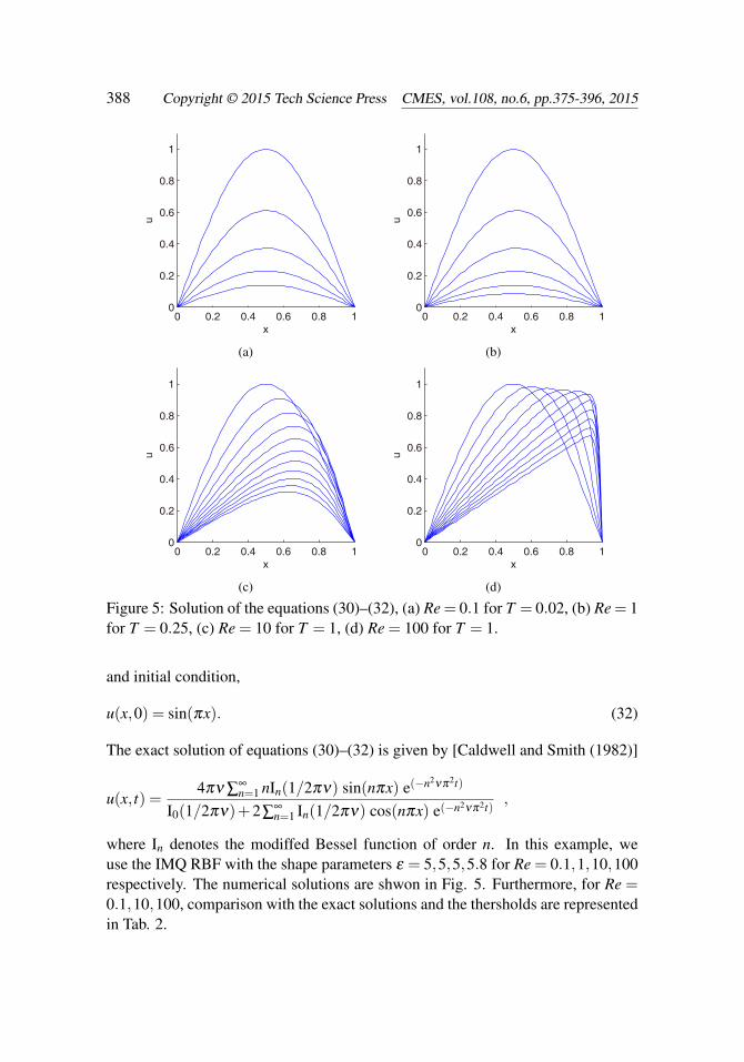
Figure 5: Solution of the equations (30)–(32), (a) Re = 0.1 for T = 0.02, (b) Re = 1for T = 0.25, (c) Re = 10 for T = 1, (d) Re = 100 for T = 1.


u(x,0) = sin(πx). (32)

The exact solution of equations (30)–(32) is given by [Caldwell and Smith (1982)]

u(x, t) =4πν ∑

∞n=1 nIn(1/2πν) sin(nπx) e(−n2νπ2t)

I0(1/2πν)+2∑∞n=1 In(1/2πν) cos(nπx) e(−n2νπ2t)

,

where In denotes the modiffed Bessel function of order n. In this example, weuse the IMQ RBF with the shape parameters ε = 5,5,5,5.8 for Re = 0.1,1,10,100respectively. The numerical solutions are shwon in Fig. 5. Furthermore, for Re =0.1,10,100, comparison with the exact solutions and the thersholds are representedin Tab. 2.


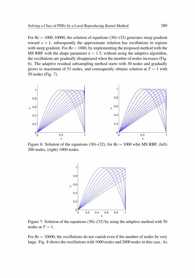
For Re = 1000,10000, the solution of equations (30)–(32) generates steep gradienttoward x = 1, subsequently the approximate solution has oscillations in regionswith steep gradient. For Re= 1000, by implementing the proposed method with theMS RBF with the shape parameter ε = 1.5, without using the adaptive algorithm,the oscillations are gradually disappeared when the number of nodes increases (Fig.6). The adaptive residual subsampling method starts with 30 nodes and graduallygrows to maximum of 53 nodes, and consequently obtains solution at T = 1 with50 nodes (Fig. 7).

0 0.5 10

0.2

0.4

0.6

0.8

1

x

u

0 0.5 10

0.2

0.4

0.6

0.8

1

x

u

Figure 6: Solution of the equations (30)–(32), for Re = 1000 whit MS RBF, (left)200 nodes, (right) 1000 nodes.

0 0.2 0.4 0.6 0.8 10

0.2

0.4

0.6

0.8

1

x

u

Figure 7: Solution of the equations (30)–(32) by using the adaptive method with 50nodes at T = 1.

For Re = 10000, the oscillations do not vanish even if the number of nodes be verylarge. Fig. 8 shows the oscillations with 1000 nodes and 2000 nodes in this case. As


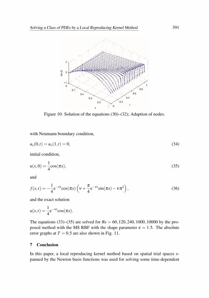
shown in Fig. 9, by using the adaptive residual subsampling algorithm and MS RBFwith ε = 1, the oscillations are disappeared at T = 1 with 108 nodes (Fig. 9). ForRe = 10000, the numerical solution has been compared with the Christie accuratesolution given in [Hon and Mao (1998)]. Absolute error graph of implementationof the proposed method for Re = 10000 is shown in Fig. 9. In addition, adaptionof nodes are shown in Fig. 10.

0 0.5 10

0.2

0.4

0.6

0.8

1

x

u

0 0.5 10

0.2

0.4

0.6

0.8

1

x

u

Figure 8: Solution of the equations (30)–(32), for Re = 10000 with MS RBF, (left)1000 nodes, (right) 2000 nodes.

0 0.2 0.4 0.6 0.8 10

0.2

0.4

0.6

0.8

1

u

x

0 0.2 0.4 0.6 0.8 10

1

2

3

4

5

6

7x 10

−3

x

Ab

so

lute

err

or

Figure 9: (left) Solution of the equations (30)–(32) for Re = 10000 with the adap-tive method, (right) Absolute error graph at x = 0, 0.05, 0.11, 0.16, 0.22, 0.27, 0.33,0.38, 0.44, 0.50, 0.55, 0.61, 0.66, 0.72, 0.77, 0.83, 0.88, 0.94, 1.

Example 4: Consider the Burgers’ equation [Pugh (1995)]

ut =−uux +νuxx + f (x, t), x ∈ [0,1], t ∈ [0,T ], (33)


Figure 10: Solution of the equations (30)–(32); Adaption of nodes.

with Neumann boundary condition,

ux(0, t) = ux(1, t) = 0, (34)

initial condition,

u(x,0) =14

cos(πx), (35)

and

f (x, t) =−14

e−νtcos(πx)(

ν +π

4e−νtsin(πx)−νπ

2), (36)

and the exact solution

u(x, t) =14

e−νtcos(πx).

The equations (33)–(35) are solved for Re = 60,120,240,1000,10000 by the pro-posed method with the MS RBF with the shape parameter ε = 1.5. The absoluteerror graphs at T = 0.5 are also shown in Fig. 11.

7 Conclusion

In this paper, a local reproducing kernel method based on spatial trial spaces s-panned by the Newton basis functions was used for solving some time-dependent


0 0.5 10

2

4

6

8x 10

−4

x

Ab

so

lute

err

or

(a) Re = 60

0 0.5 13

4

5

6

7

8

9

10x 10

−5

x

Ab

so

lute

err

or

(b) Re = 120

0 0.2 0.4 0.6 0.8 10

2

4

6

8

x 10−5

x

Ab

so

lute

err

or

(c) Re = 240

0 0.2 0.4 0.6 0.8 10

1

2

3

4x 10

−4

x

Ab

so

lute

err

or

(d) Re = 1000

0 0.2 0.4 0.6 0.8 10

2

4

6

8x 10

−5

x

Ab

so

lute

err

or

(e) Re = 10000

Figure 11: Absolute error graphs for solution of the equations (33)–(35) at T = 0.5.


PDEs. In addition, the adaptive residual subsampling algorithm was employedto correct oscillations. Numerical results show that the method works properlyfor problems with oscillatory behaviour due to steep gradients. It seems that thismethod can be applied for solving higher dimensional time dependent PDEs. Weleave this to our further work.

References

Abbasbandy, S.; Azarnavid, B.; Alhuthali, M. (2014): A shooting reproduc-ing kernel hilbert space method for multiple solutions of nonlinear boundary valueproblems. J. Comput. Appl. Math. http://dx.doi.org/10.1016/j.cam.2014.11.014.

Atluri, S.; Shen, S. (2003): The Meshless Local Petrov-Galerkin (MLPG)Method. Tech. Science Press.

Belytschko, T.; Krongauz, Y.; Organ, D.; Fleming, M.; Krysl, P. (1996): Mesh-less methods: an overview and recent developments. Comput. Methods Appl.Mech., Engrg., vol. 139, pp. 3–47.

C. Franke, R. S. (1998): Solving partial differential equations by collocationusing radial basis functions. Appl. Math. Comput., vol. 93, pp. 73–82.

Caldwell, J.; Smith, P. (1982): Solution of burgers’ equation with a large reynoldsnumber. Appl. Math. Modelling., vol. 6, pp. 381–385.

Chen, C.; Ganesh, M.; Golberg, M.; Cheng, A. (2002): Multilevel compact ra-dial basis functions based computational scheme for some elliptic problems. Com-put. Math. Appl, vol. 43, pp. 359–378.

Dong, L.; Alotaibi, A.; Mohiuddine, S.; Atluri, S. N. (2014): Computationalmethods in engineering: A variety of primal & mixed methods, with global & localinterpolations, for well-posed or ill-posed bcs. CMES Comput. Model. Eng. Sci.,vol. 99, pp. 1–85.

Driscoll, T.; Heryudono, A. (2007): Adaptive residual subsampling methods forradial basis function interpolation and collocation problems. Comput. Math. Appl,vol. 53, pp. 927–939.

Elgohary, T.; Dong, L.; Junkins, J.; Atluri, S. N. (2014): Time domain inverseproblems in nonlinear systems using collocation & radial basis functions. CMESComput. Model. Eng. Sci., vol. 100, pp. 59–84.

Gong, D.; Wei, C.; Wang, L.; Feng, L.; Wang, L. (2010): adaptive methods forcenter choosing of radial basis function interpolation: a review. Lecture Notes inComput. Sci., vol. 6377, pp. 573–580.


Han, Z.; Atluri, S. (2014): On the (meshless local petrov-galerkin) mlpg-eshelbymethod in computational finite deformation solid mechanics - part ii. CMES Com-put. Model. Eng. Sci., vol. 97, pp. 199–237.

Hon, Y.; Mao, X. (1998): An efficient numerical scheme for burgers’ equation.Appl. Math. Comput., vol. 95, pp. 37–50.

Hon, Y.; Schaback, R. (2008): Solvability of partial differential equations bymeshless kernel methods. Adv. Comput. Math., vol. 28, pp. 283–299.

Huang, W.; Ren, Y.; Russell, R. D. (1990): Multiquadrics–a scattered dataapproximation scheme with applications to computational fluid dynamics i: surfaceapproximations and partial derivative estimates. Computers Math. Appl., vol. 19,pp. 127–145.

Huang, W.; Ren, Y.; Russell, R. D. (1990): Multiquadrics–a scattered dataapproximation scheme with applications to computational fluid-dynamicsii: solu-tions to parabolic, hyperbolic and elliptic partial differential equations. ComputersMath. Appl., vol. 19, pp. 147–161.

Huang, W.; Ren, Y.; Russell, R. D. (1994): Moving mesh partial differentialequations (mmpdes) based on the equidistribution principle. SIAM J. Numer. Anal.,vol. 31, pp. 709–730.

Lee, C.; Liu, X.; Fan, S. (2003): Local multiquadric approximation for solvingboundary value problems. Comput. Mech., vol. 30, pp. 396–409.

Lin, H.; Atluri, S. (2000): Meshless local petrov-galerkin (mlpg) method forconvection-diffusion problems. CMES Comput. Model. Eng. Sci., vol. 1, pp. 45–60.

Lin, H.; Atluri, S. (2001): The meshless local petrov-galerkin (mlpg) method forsolving incompressible navier-stokes equations. CMES Comput. Model. Eng. Sci.,vol. 2, pp. 117–142.

Ling, L.; Opfe, R.; Schaback, R. (2006): Results on meshless collocation tech-niques. Eng. Anal. Bound. Elem., vol. 30, pp. 247–253.

Ling, L.; Schaback, R. (2009): An improved subspace selection algorithm formeshless collocation methods. Int. J. Numer. Meth. Engng., vol. 80, pp. 1623–1639.

Mai-Duy, N.; Tran-Cong, T. (2002): Mesh-free radial basis function networkmethods with domain decomposition for approximation of functions and numericalsolution of poisson equation. Eng. Anal. Bound. Elem., vol. 26, pp. 133–156.


Mohammadi, M.; Mokhtari, R. (2011): Solving the generalized regularizedlong wave equation on the basis of a reproducing kernel space. J. Comput. Appl.Math., vol. 235, pp. 4003–4014.

Mohammadi, M.; Mokhtari, R. (2013): A new algorithm for solving nonlinearschrödinger equation in the reproducing kernel space. Iranian J. Sci. Tech., vol.37, pp. 523–546.

Mohammadi, M.; Mokhtari, R. (2014): A reproducing kernel method for solv-ing a class of nonlinear systems of pdes. Math. Model. Anal., vol. 19, pp. 180–198.

Mohammadi, M.; Mokhtari, R.; Isfahani, F. T. (2014): Solving an inverse prob-lem for a parabolic equation with a nonlocal boundary condition in the reproducingkernel space. Iranian J. Numer. Anal. Optimization., vol. 4, pp. 57–76.

Mohammadi, M.; Mokhtari, R.; Panahipour, H. (2013): A galerkin-reproducing kernel method: application to the 2d nonlinear coupled burgers’ e-quations. Eng. Anal. Bound. Elem., vol. 37, pp. 1642–1652.

Mohammadi, M.; Mokhtari, R.; Panahipour, H. (2014): Solving two parabolicinverse problems with a nonlocal boundary condition in the reproducing kernelspace. Appl. Comput. Math., vol. 13, pp. 91–106.

Mohammadi, M.; Mokhtari, R.; Schaback, R. (2014): A meshless method forsolving the 2d brusselator reaction-diffusion system. CMES: Comput. Model. Eng.Sci., vol. 101, pp. 113–138.

Mokhtari, R.; Isfahani, F. T.; Mohammadi, M. (2012): Reproducing kernelmethod for solving nonlinear differential-difference equations. Abstr. Appl. Anal.,vol. 2012, pp. 1–10.

Muller, S.; Schaback, R. (2009): A newton basis for kernel spaces. J. Approx.Theory., vol. 161, pp. 645–655.

Pazouki, M.; Schaback, R. (2011): Bases for kernel-based spaces. J. Comput.Appl. Math., vol. 236, pp. 575–588.

Pugh, S. (1995): Finite element approximations of burgers’ equation.

Scahabck, R. (2011): Kernel-based meshless methods. Lecture Note, Gottingen.http://num.math.unigoettingen.de/schaback/teaching/AV2.pdf.

Schaback, R. (1995): Error estimates and condition numbers for radial basisfunction interpolation. Adv. Comput. Math., vol. 3, pp. 251–264.

Schaback, R. (2015): A computational tool for comparing all linear pde solvers.Adv. Comput. Math., vol. 41, pp. 333–355.

Wendland, H. (2005): Scattered Data Approximation. Cambridge UniversityPress.

Documents

Solving a Class of PDEs by a Local Reproducing Kernel Method … · Method with An Adaptive Residual Subsampling Technique H. Raﬁeayan Zadeh1, ... and Russell (1990a); Huang, Ren,