Solvent reorganization energy of electron-transfer reactions in polar solvents

Solvent reorganization energy of electron-transfer reactions in polarsolventsDmitry V. Matyushov Citation: J. Chem. Phys. 120, 7532 (2004); doi: 10.1063/1.1676122 View online: http://dx.doi.org/10.1063/1.1676122 View Table of Contents: http://jcp.aip.org/resource/1/JCPSA6/v120/i16 Published by the American Institute of Physics. Additional information on J. Chem. Phys.Journal Homepage: http://jcp.aip.org/ Journal Information: http://jcp.aip.org/about/about_the_journal Top downloads: http://jcp.aip.org/features/most_downloaded Information for Authors: http://jcp.aip.org/authors

Downloaded 07 May 2013 to 128.143.22.132. This article is copyrighted as indicated in the abstract. Reuse of AIP content is subject to the terms at: http://jcp.aip.org/about/rights_and_permissions

http://jcp.aip.org/?ver=pdfcov

http://oasc12039.247realmedia.com/RealMedia/ads/click_lx.ads/www.aip.org/pt/adcenter/pdfcover_test/L-37/1117033590/x01/AIP-PT/Goodfellow_JCPCoverPg_042413/NEW_Goodfellow_banner.jpeg/6c527a6a7131454a5049734141754f37?x

http://jcp.aip.org/search?sortby=newestdate&q=&searchzone=2&searchtype=searchin&faceted=faceted&key=AIP_ALL&possible1=Dmitry V. Matyushov&possible1zone=author&alias=&displayid=AIP&ver=pdfcov


http://link.aip.org/link/doi/10.1063/1.1676122?ver=pdfcov

http://jcp.aip.org/resource/1/JCPSA6/v120/i16?ver=pdfcov

http://www.aip.org/?ver=pdfcov


http://jcp.aip.org/about/about_the_journal?ver=pdfcov

http://jcp.aip.org/features/most_downloaded?ver=pdfcov

http://jcp.aip.org/authors?ver=pdfcov

Solvent reorganization energy of electron-transfer reactionsin polar solvents

Dmitry V. Matyushova)

Department of Chemistry and Biochemistry and the Center for the Early Events in Photosynthesis,Arizona State University, Tempe, Arizona 85287-1604

~Received 26 September 2003; accepted 21 January 2004!

A microscopic theory of solvent reorganization energy in polar molecular solvents is developed. Thetheory represents the solvent response as a combination of the density and polarization fluctuationsof the solvent given in terms of the density and polarization structure factors. A fully analyticalformulation of the theory is provided for a solute of arbitrary shape with an arbitrary distribution ofcharge. A good agreement between the analytical procedure and the results of Monte Carlosimulations of model systems is achieved. The reorganization energy splits into the contributionsfrom density fluctuations and polarization fluctuations. The polarization part is dominated bylongitudinal polarization response. The density part is inversely proportional to temperature. Thedependence of the solvent reorganization energy on the solvent dipole moment and refractive indexis discussed. ©2004 American Institute of Physics.@DOI: 10.1063/1.1676122#

I. INTRODUCTION

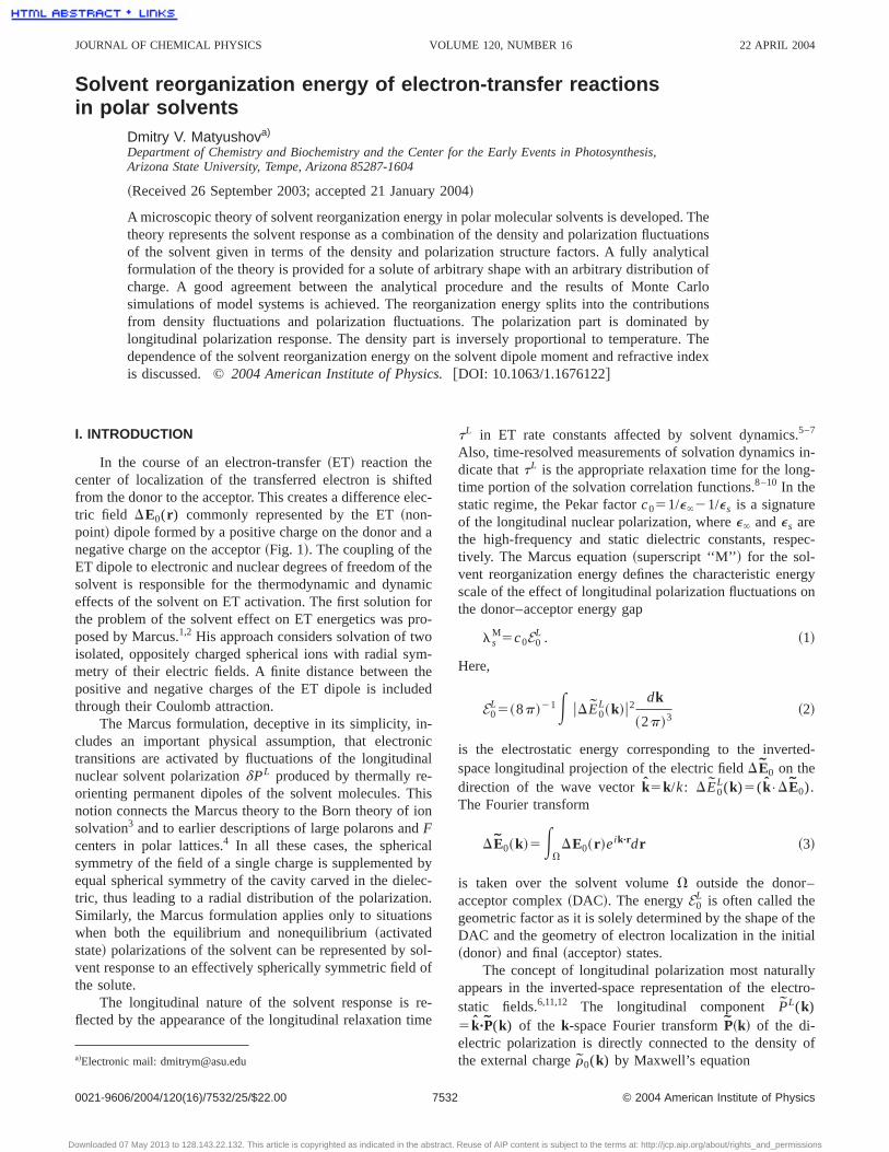
In the course of an electron-transfer~ET! reaction thecenter of localization of the transferred electron is shiftedfrom the donor to the acceptor. This creates a difference elec-tric field DE0(r ) commonly represented by the ET~non-point! dipole formed by a positive charge on the donor and anegative charge on the acceptor~Fig. 1!. The coupling of theET dipole to electronic and nuclear degrees of freedom of thesolvent is responsible for the thermodynamic and dynamiceffects of the solvent on ET activation. The first solution forthe problem of the solvent effect on ET energetics was pro-posed by Marcus.1,2 His approach considers solvation of twoisolated, oppositely charged spherical ions with radial sym-metry of their electric fields. A finite distance between thepositive and negative charges of the ET dipole is includedthrough their Coulomb attraction.

The Marcus formulation, deceptive in its simplicity, in-cludes an important physical assumption, that electronictransitions are activated by fluctuations of the longitudinalnuclear solvent polarizationdPL produced by thermally re-orienting permanent dipoles of the solvent molecules. Thisnotion connects the Marcus theory to the Born theory of ionsolvation3 and to earlier descriptions of large polarons andFcenters in polar lattices.4 In all these cases, the sphericalsymmetry of the field of a single charge is supplemented byequal spherical symmetry of the cavity carved in the dielec-tric, thus leading to a radial distribution of the polarization.Similarly, the Marcus formulation applies only to situationswhen both the equilibrium and nonequilibrium~activatedstate! polarizations of the solvent can be represented by sol-vent response to an effectively spherically symmetric field ofthe solute.

The longitudinal nature of the solvent response is re-flected by the appearance of the longitudinal relaxation time

tL in ET rate constants affected by solvent dynamics.5–7

Also, time-resolved measurements of solvation dynamics in-dicate thattL is the appropriate relaxation time for the long-time portion of the solvation correlation functions.8–10 In thestatic regime, the Pekar factorc051/e`21/es is a signatureof the longitudinal nuclear polarization, wheree` andes arethe high-frequency and static dielectric constants, respec-tively. The Marcus equation~superscript ‘‘M’’! for the sol-vent reorganization energy defines the characteristic energyscale of the effect of longitudinal polarization fluctuations onthe donor–acceptor energy gap

lsM5c0E0

L . ~1!

Here,

E0L5~8p!21E uDE0

L~k!u2dk

~2p!3~2!

is the electrostatic energy corresponding to the inverted-space longitudinal projection of the electric fieldDE0 on thedirection of the wave vectork5k/k: DE0

L(k)5( k•DE0).The Fourier transform

DE0~k!5EV

DE0~r !eik"rdr ~3!

is taken over the solvent volumeV outside the donor–acceptor complex~DAC!. The energyE0

L is often called thegeometric factor as it is solely determined by the shape of theDAC and the geometry of electron localization in the initial~donor! and final~acceptor! states.

The concept of longitudinal polarization most naturallyappears in the inverted-space representation of the electro-static fields.6,11,12 The longitudinal componentPL(k)5 k"P(k) of the k-space Fourier transformP~k! of the di-electric polarization is directly connected to the density ofthe external charger0(k) by Maxwell’s equationa!Electronic mail: [email protected]

JOURNAL OF CHEMICAL PHYSICS VOLUME 120, NUMBER 16 22 APRIL 2004

75320021-9606/2004/120(16)/7532/25/$22.00 © 2004 American Institute of Physics


http://dx.doi.org/10.1063/1.1676122

PL~k!5S 121

esD i r0~k!

k. ~4!

This connection substantially simplifies all the electrostaticcalculations in cases whenPL5 P. In the direct space, thiscondition implies that the polarization of the dielectric sur-rounding a solute can be directly connected to the vacuumsource field:

P5PL51

4p S 121

esDDE0 . ~5!

This relation also implies that Maxwell’s dielectric displace-mentD within the dielectric is equal to the source fieldDE0 :

D5DE0 . ~6!

The free energy of solvation,Fsolv, can then be easily calcu-lated from the vacuum external field by integration of theelectrostatic energy density over the volume occupied by thesolvent:

Fsolv521

2 EVD~r !•P~r !dr

521

8p S 121

esD E

VDE0~r !2dr . ~7!

As was recognized by Kharkatset al.13 Eq. ~6! is satis-fied only when the boundary of the cavity cut off by theDAC from the solvent coincides with an equipotential sur-face of the charge distribution within the cavity. When this isnot the case, the lines of the source field are not normal tothe cavity surface resulting inDÞDE0 ~Fig. 1!. The dielec-tric polarization is then determined by both the source chargeand the apparent surface charge,14 and Eq.~5! does not holdany more. In the direct-space representation, this means thatdielectric displacement should be sought by solving the Pois-son equation with the boundary conditions set up by thedielectric cavity. In thek-space description, this implies thatthe polarization is not solely given by the source charge dis-

tribution @Eq. ~4!# and the transverse polarization componentPT5uP2 k( k"P)u contributes to the solvent response. It wasargued that a cavity containing an ET dipole always crossesits equipotential surfaces~Fig. 1! and transverse polarizationcannot be neglected.13 Both the longitudinal and transversecomponents of the solvent polarization then affect the energygap DE between the acceptor and donor electronic states.This symmetry change broadens the spectrum of solvent col-lective modes activating ET from purely longitudinal, as inthe case of large polarons, to longitudinal,PL, and trans-verse,PT, polarization modes~Figs. 1 and 2!.

The importance of both the longitudinal and transversepolarization modes is well recognized in current continuumformulations of the ET theory which search for a solution ofthe Poisson equation for the ET dipole in a cavity of arbitraryshape.15–17 Indeed, the calculation of electrostatic energy ofthe ET dipole within ellipsoidal cavities shows that the sol-vent reorganization energyls cannot be separated into a sol-vent ~e.g., Pekar factor! and geometric (E0

L) factors. The de-pendence ofls on the solvent dielectric constant is entangledwith the cavity shape.18 Therefore, both longitudinal andtransverse polarizations contribute to the electric field of thesolvent interacting with solute’s charges. At this point, thecontinuum electrostatic calculations come in contradiction tothe original Marcus concept and studies of ET dynamics bothpointing to the longitudinal polarization as the principal sol-vent mode driving electronic transitions.

The recent two decades have seen an increasing interestin the development of microscopic theories of ETreorganization.19–29Theoretical models are usually based oneither liquid-state theories of solvation19–24,29or direct com-puter simulations of the reorganization energy25,30 and ETfree energy surfaces.26–28,31 This development has recog-nized the fact that the coupling of macroscopic fluctuationsof dipolar polarization to the ET dipole is not the onlymechanism of ET activation, and other interaction potentialsand molecular modes may be active as well. Two major ex-tensions of the original Marcus concept have been suggested:~i! a distinction between rotational and translational modesof the solvent affecting ET activation20,32 and solvationdynamics33,34 and ~ii ! the role of higher solvent multi-

FIG. 1. ET dipole formed by a negative charge on the acceptor~A! and apositive charge on the donor~D!. The dashed lines show equipotential sur-faces of the ET dipole which cross the cavity surface~solid line!. The di-electric displacementD is then nonequal to the source fieldDE0 . For thatreason the projection of the solvent polarizationP on the direction of thesource field is not equal toPL given by Eq.~5!.

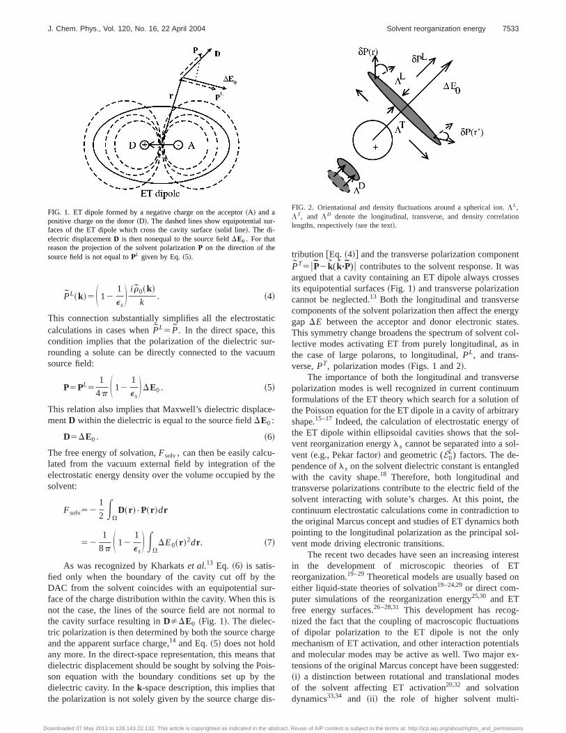
FIG. 2. Orientational and density fluctuations around a spherical ion.LL,LT, and LD denote the longitudinal, transverse, and density correlationlengths, respectively~see the text!.

7533J. Chem. Phys., Vol. 120, No. 16, 22 April 2004 Solvent reorganization energy


poles for reactions in weakly polar and nondipolarsolvents.21,22,30,35–37

On short time scales of solvation dynamics, when long-range multipolar correlations are not yet established, bothrotations and translations participate in purely ballisticmotion.33 The dynamics of solvent response due to transla-tions and rotations becomes, however, distinctly different ondiffusional time scales when the long-range orientational cor-relations become active.34 Finally, in the static regime, whenthe time scale of the process of interest (kET

21 for ET, wherekET is the ET rate constant! is much larger than the charac-teristic time scales of molecular motions, the difference incorrelation lengths of the density~translations! and orienta-tional ~rotations! collective modes is reflected in a muchstronger temperature dependence of the density componentof the solvent reorganization energy.20 The same is true notonly for charge–dipole solute–solvent coupling, but also forother interaction potentials depending on the coordinates ofthe solvent molecules~induction and dispersion forces!.38,39

Fluctuations of all these potentials, caused by density fluc-tuations of the solvent, lead to a pronounced temperaturedependence ofls . The entropy of solvent reorganization isthus dominated by short-range density fluctuations and notby long-range orientational fluctuations. The total reorgani-zation entropy is positive as confirmed by experiment,40–44

in contrast to a negative entropy predicted by dielectric cav-ity models.

An account for higher solvent multipoles, in particularfor solvent quadrupoles coupled to the gradient of the soluteelectric field, is necessary for solvents composed of mol-ecules with small or zero dipole moment.21,22,35,36This modi-fication of the theory goes necessarily beyond dielectricmodels since the dielectric constant reflects molecular qua-drupoles only indirectly~through the Kirkwood factor!.45,46

The charge–quadrupole interaction decays faster with thedistance than the charge–dipole interaction. The relative im-portance of quadrupole moments in solvents with nonzerodipoles depends therefore on the solute size. For commonlylarge donor and acceptor units employed in ET studies, thequadrupolar contribution to the solvent reorganization energyis small in all but nondipolar solvents, and the quadrupolarsolvation energy can be safely dropped for ET in evenweakly polar solvents.30 We therefore focus in this study ondipolar polarization fluctuations, reserving a relatively nar-row class of nondipolar solvents to future work.

The present state of the problem of calculating the sol-vent reorganization energy in polar solvents may be summa-rized as follows. Dielectric continuum models offer signifi-cant flexibility in treating molecular solutes of complexgeometries. A solution of the Poisson equation for a molecu-lar cavity includes both the longitudinal and transverse po-larization components. Procedures of defining cavities are,however, ambiguous and the calculation results are very sen-sitive to the choice of the dielectric cavity. In addition, it isnot clear whether the equal account of two types of polariza-tion by the Poisson equation is consistent with quite differenttime and length scales of these two modes on the micro-scopic level~Fig. 2!. On the other side of the theoreticalspectrum, molecular solvation theories incorporate a more

realistic description of molecular dynamics and thermody-namics. Existing models are, however, limited in their abilityto treat large solutes of complex molecular shape. Both thelongitudinal and transverse polarization components were in-cluded in the solvent response for a spherical dipolarsolute.36,47 That model has been used to calculate steady-state optical band shapes for dipolar chromophores in abroad range of solvent polarities30 and has been applied tocalculate entropies of ET activation.37,48The effective radiusof the solute is not, however, specified in the model andshould be fitted to some experimental observable; the Stokesshift30,42 and the equilibrium energy gap37 have been used inrecent applications. The transverse polarization is often ne-glected in microscopic models of the energetics20–22 anddynamics6 of ET. It is not included in the RISMcalculations21,22 due to the way the RISM approximation isformulated.49 The combination of limitations in treating sol-ute molecular geometry with neglect of some important col-lective polarization modes present in molecular solvents ob-viously narrows the range of applications of molecularsolvation models. The development of an effective algorithmapplicable to an arbitrary geometry of the DAC with fullaccount of solvent polarization modes is a pressing need forapplications, especially in the realm of redox chemistry ofbiopolymers. This paper presents the first step in this direc-tion.

Various levels of complexity may be chosen for molecu-lar modeling of the solvent effect. Realistic intermolecularpotentials with partial molecular and atomic charges are of-ten used in computer simulations. These approaches providea very detailed picture of the local solute–solvent structure.These models are, however, hard to employ in formal theo-ries. Furthermore, a still existing ambiguity of treating long-range Coulomb forces in computer simulations, especially atinfinite dilution of large solutes common for biological ap-plications, leaves open the question of the ability of finite-size simulations to grasp the long-range polarization struc-ture of the solvent around a molecular solute. On the otherhand, a tremendous success of continuum models in treatingthe Gibbs energy of solvation50 suggests that a substantialportion of significant physics is accounted for even on thecontinuum level of the theory. The dielectric continuum ap-proach fails to describe short-range solvation effects re-flected by such properties as the entropy of solvation,20,51

quadrupolar solvation,21,22,30,35–37,46 and specificinteractions.52 However, the formalism of responsefunctions,53–56 providing a reduced description of the com-plex molecular problem, is a valuable component of the con-tinuum approach which can be extended to include variousmolecular modes and molecular dimensions. This is the basicapproach adopted in this paper. The formalism for the calcu-lation of the reorganization energy is given in terms ofk-dependent density57 and polarization58,59 structure factorsof the solvent which are incorporated into the theory to formthe nonlocal polarity response functions depending on boththe solvent and solute geometry. For convenience, we willrefer to the present formulation as to the nonlocal responsefunction theory ~NRFT!. The analytical calculations for

7534 J. Chem. Phys., Vol. 120, No. 16, 22 April 2004 Dmitry V. Matyushov


model solute geometries and computer simulations are per-formed for the model solvent of multipolar hard spheres.

The model of polarizable hard spheres with centered mo-lecular multipoles has the desired universality in a sense thatit may be parametrized to describe a broad list of molecularsolvents60–63on the one hand and incorporates the main ther-mal molecular motions of real solvents—rotations andtranslations—on the other. An additional advantage is thatthe solvent molecular polarizability, which is often very ex-pensive for computer simulations,64,65 is incorporatedthrough a renormalized solvent dipole.45,66–68The sphericalapproximation for molecular cores of the solvent moleculesmay seem to be an oversimplification, but there are strongarguments for its ability to account for nonspecific solventeffects on chemical thermodynamics and solvation.69 Recentapplications of the model have demonstrated its ability toaccurately describe activation37,48,70 and spectroscopy30 ofcharge-transfer transitions. Although the calculations andsimulations are done here for the model of dipolar solventmolecules, the formalism is not limited by this assumption.The theory is formulated in terms of density and polarizationstructure factors of the pure solvent and those for an arbitrarymolecular solvent can be used in the calculations.

The results of microscopic calculations are comparedthroughout the paper to the continuum limit which followsfrom the NRFT whenk dependence is neglected in the sol-vent response functions. The notion of continuum solvationapplies to thedielectric continuumdescription as first formu-lated by Born,3 Onsager,71 and Kirkwood.72 A few recentcontinuumsolvation models73–75incorporate molecular prop-erties which are not reflected by the static and high-frequency dielectric constants of the solvent. These con-tinuum approximations are not considered here as the NRFTincludes only dielectric continuum as its limiting case.

The rest of the paper is organized as follows: The nextsection provides a compilation of critical properties of thesolvent reorganization energy illustrated by the results fromMonte Carlo~MC! simulations. This compilation sets up alist of requirements which an accurate analytical model ofsolvent reorganization should meet. The theory developmentstarts with the instantaneous free energies depending on thenuclear configuration of the system as given in Sec. III. Theformulation of the theory of solvent reorganization is pre-sented in Sec. IV. This is followed by the development of ananalytical approximation to calculate the polarization struc-ture factors of a pure polar solvent in Sec. V. A description ofthe numerical algorithm and a comparison between the ana-lytical theory and simulations are presented in Sec. VI. Thepaper concludes with a short summary in Sec. VII.

II. CONCEPTUAL FORMULATION

A. Solvent reorganization energyin the linear response approximation

Radiationless transitions are activated by thermal nuclearfluctuations creating the resonance of the donor and acceptorelectronic levels. The rate constant of ET,kET , is propor-tional to the probability of a nuclear configuration leading to

zero energy gapDE50 between the donor and acceptorelectronic states,

kET}Pi~0!. ~8!

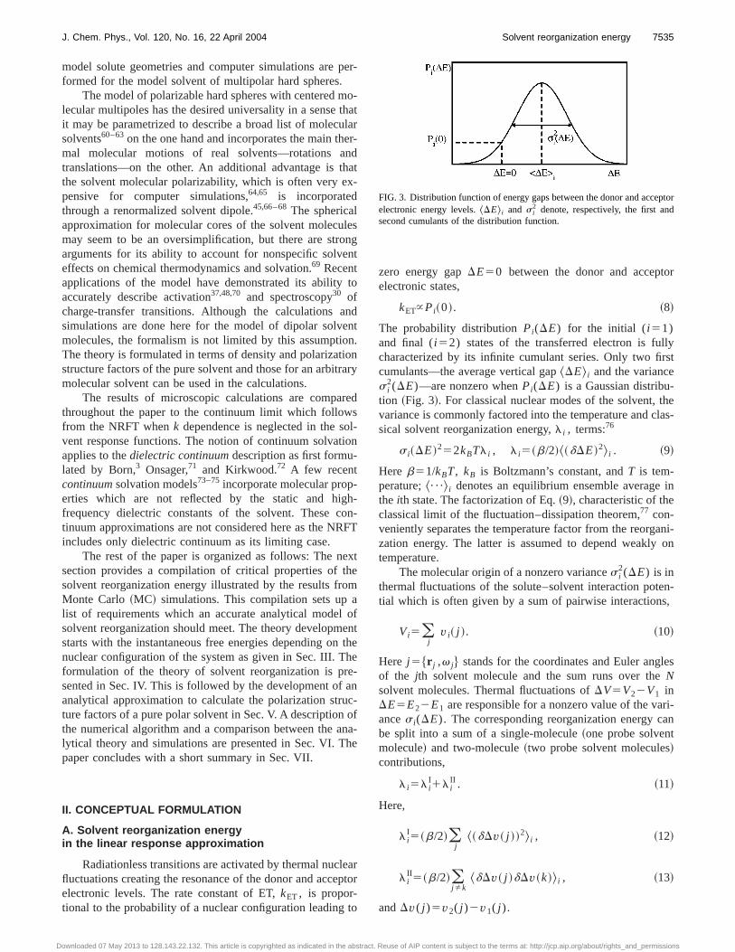
The probability distributionPi(DE) for the initial (i 51)and final (i 52) states of the transferred electron is fullycharacterized by its infinite cumulant series. Only two firstcumulants—the average vertical gap^DE& i and the variances i

2(DE)—are nonzero whenPi(DE) is a Gaussian distribu-tion ~Fig. 3!. For classical nuclear modes of the solvent, thevariance is commonly factored into the temperature and clas-sical solvent reorganization energy,l i , terms:76

s i~DE!252kBTl i , l i5~b/2!^~dDE!2& i . ~9!

Here b51/kBT, kB is Boltzmann’s constant, andT is tem-perature; ¯& i denotes an equilibrium ensemble average inthe ith state. The factorization of Eq.~9!, characteristic of theclassical limit of the fluctuation–dissipation theorem,77 con-veniently separates the temperature factor from the reorgani-zation energy. The latter is assumed to depend weakly ontemperature.

The molecular origin of a nonzero variances i2(DE) is in

thermal fluctuations of the solute–solvent interaction poten-tial which is often given by a sum of pairwise interactions,

Vi5(j

v i~ j !. ~10!

Here j 5$r j ,v j% stands for the coordinates and Euler anglesof the jth solvent molecule and the sum runs over theNsolvent molecules. Thermal fluctuations ofDV5V22V1 inDE5E22E1 are responsible for a nonzero value of the vari-ances i(DE). The corresponding reorganization energy canbe split into a sum of a single-molecule~one probe solventmolecule! and two-molecule~two probe solvent molecules!contributions,

l i5l iI1l i

II . ~11!

Here,

l iI5~b/2!(

j^~dDv~ j !!2& i , ~12!

l iII5~b/2!(

j Þk^dDv~ j !dDv~k!& i , ~13!

andDv( j )5v2( j )2v1( j ).

FIG. 3. Distribution function of energy gaps between the donor and acceptorelectronic energy levels.DE& i and s i

2 denote, respectively, the first andsecond cumulants of the distribution function.



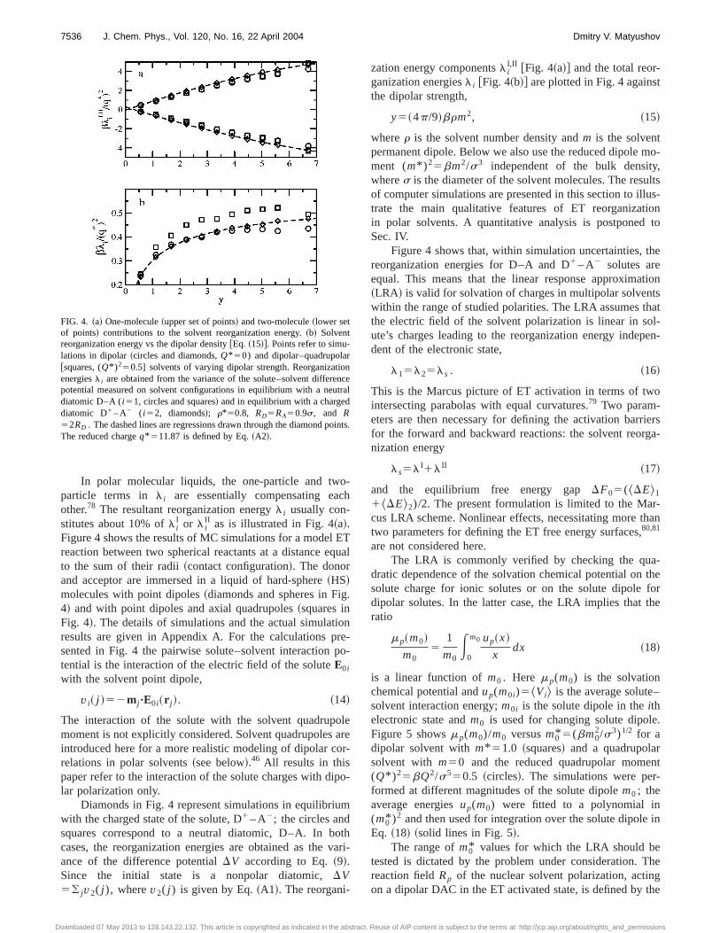
In polar molecular liquids, the one-particle and two-particle terms in l i are essentially compensating eachother.78 The resultant reorganization energyl i usually con-stitutes about 10% ofl i

I or l iII as is illustrated in Fig. 4~a!.

Figure 4 shows the results of MC simulations for a model ETreaction between two spherical reactants at a distance equalto the sum of their radii~contact configuration!. The donorand acceptor are immersed in a liquid of hard-sphere~HS!molecules with point dipoles~diamonds and spheres in Fig.4! and with point dipoles and axial quadrupoles~squares inFig. 4!. The details of simulations and the actual simulationresults are given in Appendix A. For the calculations pre-sented in Fig. 4 the pairwise solute–solvent interaction po-tential is the interaction of the electric field of the soluteE0i

with the solvent point dipole,

v i~ j !52mj "E0i~r j !. ~14!

The interaction of the solute with the solvent quadrupolemoment is not explicitly considered. Solvent quadrupoles areintroduced here for a more realistic modeling of dipolar cor-relations in polar solvents~see below!.46 All results in thispaper refer to the interaction of the solute charges with dipo-lar polarization only.

Diamonds in Fig. 4 represent simulations in equilibriumwith the charged state of the solute, D1 – A2; the circles andsquares correspond to a neutral diatomic, D–A. In bothcases, the reorganization energies are obtained as the vari-ance of the difference potentialDV according to Eq.~9!.Since the initial state is a nonpolar diatomic,DV5( jv2( j ), wherev2( j ) is given by Eq.~A1!. The reorgani-

zation energy componentsl iI,II @Fig. 4~a!# and the total reor-

ganization energiesl i @Fig. 4~b!# are plotted in Fig. 4 againstthe dipolar strength,

y5~4p/9!brm2, ~15!

wherer is the solvent number density andm is the solventpermanent dipole. Below we also use the reduced dipole mo-ment (m* )25bm2/s3 independent of the bulk density,wheres is the diameter of the solvent molecules. The resultsof computer simulations are presented in this section to illus-trate the main qualitative features of ET reorganizationin polar solvents. A quantitative analysis is postponed toSec. IV.

Figure 4 shows that, within simulation uncertainties, thereorganization energies for D–A and D1 – A2 solutes areequal. This means that the linear response approximation~LRA! is valid for solvation of charges in multipolar solventswithin the range of studied polarities. The LRA assumes thatthe electric field of the solvent polarization is linear in sol-ute’s charges leading to the reorganization energy indepen-dent of the electronic state,

l15l25ls . ~16!

This is the Marcus picture of ET activation in terms of twointersecting parabolas with equal curvatures.79 Two param-eters are then necessary for defining the activation barriersfor the forward and backward reactions: the solvent reorga-nization energy

ls5l I1l II ~17!

and the equilibrium free energy gapDF05(^DE&1

1^DE&2)/2. The present formulation is limited to the Mar-cus LRA scheme. Nonlinear effects, necessitating more thantwo parameters for defining the ET free energy surfaces,80,81

are not considered here.The LRA is commonly verified by checking the qua-

dratic dependence of the solvation chemical potential on thesolute charge for ionic solutes or on the solute dipole fordipolar solutes. In the latter case, the LRA implies that theratio

mp~m0!

m05

1

m0E

0

m0 up~x!

xdx ~18!

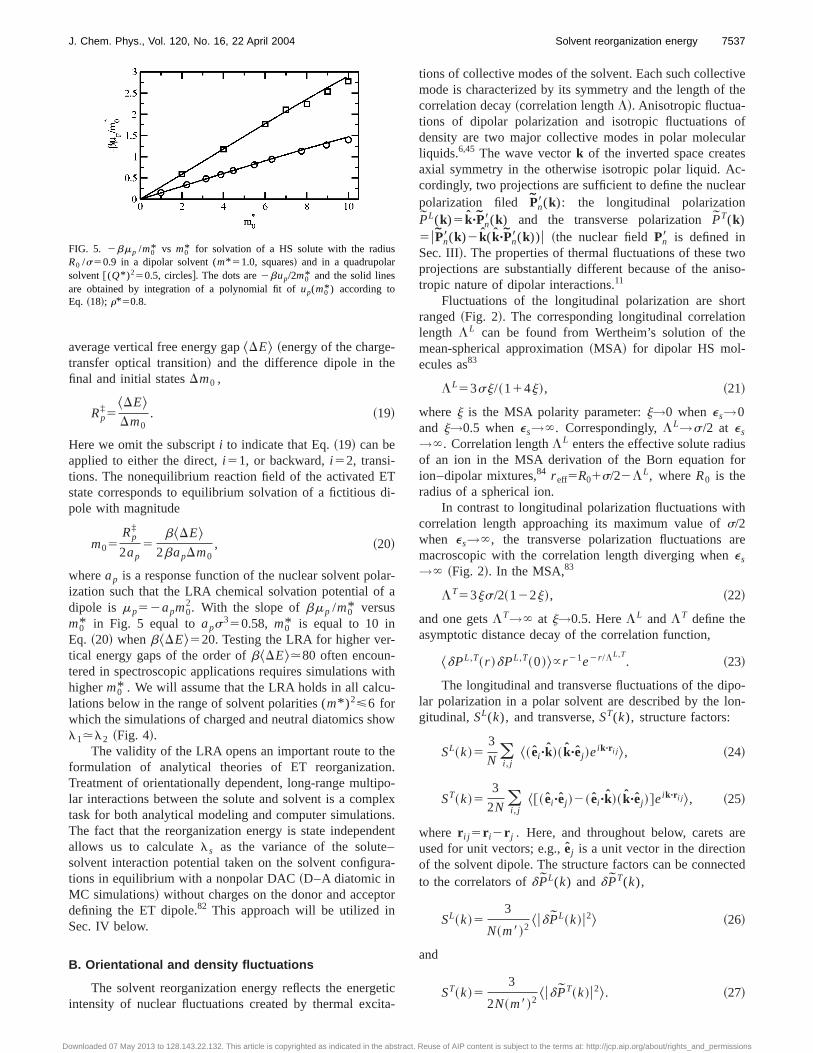
is a linear function ofm0 . Here mp(m0) is the solvationchemical potential andup(m0i)5^Vi& is the average solute–solvent interaction energy;m0i is the solute dipole in theithelectronic state andm0 is used for changing solute dipole.Figure 5 showsmp(m0)/m0 versusm0* 5(bm0

2/s3)1/2 for adipolar solvent withm* 51.0 ~squares! and a quadrupolarsolvent with m50 and the reduced quadrupolar moment(Q* )25bQ2/s550.5 ~circles!. The simulations were per-formed at different magnitudes of the solute dipolem0 ; theaverage energiesup(m0) were fitted to a polynomial in(m0* )2 and then used for integration over the solute dipole inEq. ~18! ~solid lines in Fig. 5!.

The range ofm0* values for which the LRA should betested is dictated by the problem under consideration. Thereaction fieldRp of the nuclear solvent polarization, actingon a dipolar DAC in the ET activated state, is defined by the

FIG. 4. ~a! One-molecule~upper set of points! and two-molecule~lower setof points! contributions to the solvent reorganization energy.~b! Solventreorganization energy vs the dipolar density@Eq. ~15!#. Points refer to simu-lations in dipolar~circles and diamonds,Q* 50) and dipolar–quadrupolar@squares, (Q* )250.5] solvents of varying dipolar strength. Reorganizationenergiesl i are obtained from the variance of the solute–solvent differencepotential measured on solvent configurations in equilibrium with a neutraldiatomic D–A (i 51, circles and squares! and in equilibrium with a chargeddiatomic D1 – A2 ( i 52, diamonds!; r*50.8, RD5RA50.9s, and R52RD . The dashed lines are regressions drawn through the diamond points.The reduced chargeq* 511.87 is defined by Eq.~A2!.



average vertical free energy gap^DE& ~energy of the charge-transfer optical transition! and the difference dipole in thefinal and initial statesDm0 ,

Rp‡5

^DE&Dm0

. ~19!

Here we omit the subscripti to indicate that Eq.~19! can beapplied to either the direct,i 51, or backward,i 52, transi-tions. The nonequilibrium reaction field of the activated ETstate corresponds to equilibrium solvation of a fictitious di-pole with magnitude

m05Rp

‡

2ap5

b^DE&2bapDm0

, ~20!

whereap is a response function of the nuclear solvent polar-ization such that the LRA chemical solvation potential of adipole is mp52apm0

2. With the slope ofbmp /m0* versusm0* in Fig. 5 equal toaps350.58, m0* is equal to 10 inEq. ~20! whenb^DE&520. Testing the LRA for higher ver-tical energy gaps of the order ofb^DE&.80 often encoun-tered in spectroscopic applications requires simulations withhigherm0* . We will assume that the LRA holds in all calcu-lations below in the range of solvent polarities (m* )2<6 forwhich the simulations of charged and neutral diatomics showl1.l2 ~Fig. 4!.

The validity of the LRA opens an important route to theformulation of analytical theories of ET reorganization.Treatment of orientationally dependent, long-range multipo-lar interactions between the solute and solvent is a complextask for both analytical modeling and computer simulations.The fact that the reorganization energy is state independentallows us to calculatels as the variance of the solute–solvent interaction potential taken on the solvent configura-tions in equilibrium with a nonpolar DAC~D–A diatomic inMC simulations! without charges on the donor and acceptordefining the ET dipole.82 This approach will be utilized inSec. IV below.

B. Orientational and density fluctuations

The solvent reorganization energy reflects the energeticintensity of nuclear fluctuations created by thermal excita-

tions of collective modes of the solvent. Each such collectivemode is characterized by its symmetry and the length of thecorrelation decay~correlation lengthL!. Anisotropic fluctua-tions of dipolar polarization and isotropic fluctuations ofdensity are two major collective modes in polar molecularliquids.6,45 The wave vectork of the inverted space createsaxial symmetry in the otherwise isotropic polar liquid. Ac-cordingly, two projections are sufficient to define the nuclearpolarization filed Pn8(k): the longitudinal polarizationPL(k)5 k"Pn8(k) and the transverse polarizationPT(k)5uPn8(k)2 k( k"Pn8(k))u ~the nuclear fieldPn8 is defined inSec. III!. The properties of thermal fluctuations of these twoprojections are substantially different because of the aniso-tropic nature of dipolar interactions.11

Fluctuations of the longitudinal polarization are shortranged~Fig. 2!. The corresponding longitudinal correlationlength LL can be found from Wertheim’s solution of themean-spherical approximation~MSA! for dipolar HS mol-ecules as83

LL53sj/~114j!, ~21!

wherej is the MSA polarity parameter:j→0 whenes→0and j→0.5 whenes→`. Correspondingly,LL→s/2 at es

→`. Correlation lengthLL enters the effective solute radiusof an ion in the MSA derivation of the Born equation forion–dipolar mixtures,84 r eff5R01s/22LL, whereR0 is theradius of a spherical ion.

In contrast to longitudinal polarization fluctuations withcorrelation length approaching its maximum value ofs/2when es→`, the transverse polarization fluctuations aremacroscopic with the correlation length diverging whenes

→` ~Fig. 2!. In the MSA,83

LT53js/2~122j!, ~22!

and one getsLT→` at j→0.5. HereLL andLT define theasymptotic distance decay of the correlation function,

^dPL,T~r !dPL,T~0!&}r 21e2r /LL,T. ~23!

The longitudinal and transverse fluctuations of the dipo-lar polarization in a polar solvent are described by the lon-gitudinal,SL(k), and transverse,ST(k), structure factors:

SL~k!53

N (i , j

^~ ei "k!~ k"ej !eik"r i j &, ~24!

ST~k!53

2N (i , j

^@~ ei "ej !2~ ei "k!~ k"ej !#eik"r i j &, ~25!

where r i j 5r i2r j . Here, and throughout below, carets areused for unit vectors; e.g.,ej is a unit vector in the directionof the solvent dipole. The structure factors can be connectedto the correlators ofd PL(k) andd PT(k),

SL~k!53

N~m8!2ûd PL~k!u2& ~26!

and

ST~k!53

2N~m8!2ûd PT~k!u2&. ~27!

FIG. 5. 2bmp /m0* vs m0* for solvation of a HS solute with the radiusR0 /s50.9 in a dipolar solvent (m* 51.0, squares! and in a quadrupolarsolvent@(Q* )250.5, circles#. The dots are2bup/2m0* and the solid linesare obtained by integration of a polynomial fit ofup(m0* ) according toEq. ~18!; r*50.8.



In Eqs.~24!–~27!, the average~¯! is taken over the equilib-rium configurations of the pure solvent ofN molecules andm8 is the liquid-state dipole moment of the solvent mol-ecules~see Sec. III below!.

The connection between the microscopically definedstructure factors and macroscopic dielectric functions of apolarizable solvent involves some mean-field arguments.11

The longitudinal and transverse macroscopic response func-tions can be defined in terms of correlators of the total po-larization of the solvent:

Pt5Pn1Pe , ~28!

wherePn andPe are the nuclear and electronic polarization,respectively. The longitudinal and transverse correlators arethen given by the relations

x tL5

1

4p~12es

21!5b

Vlimk→0

ûd PtL~k!u2&,

~29!

x tT5

1

2p~es21!5

b

Vlimk→0

ûd PtT~k!u2&,

whereV is the solvent volume. The above average can betaken in the mean-field approximation for the solvent-induced dipoles:

b

Vlimk→0

ûd PtL~k!u2&53rsLa1@brm2~sL!2/3#SL~0!,

~30!b

Vlimk→0

ûd PtT~k!u2&56rsTa1@2brm2~sT!2/3#ST~0!,

where the factorssL andsT account for the renormalizationof the vacuum solvent polarizabilitya and dipole momentmby the self-consistent field of the induced dipoles.85 From thecondition thates5e` at m50 one getssL5(e`12)/3e`

and sT5(e`12)/3, which leads to the following relationbetween thek50 values of two structure factors:

SL~0!

ST~0!5

e`

es. ~31!

Equation ~31! was obtained previously by Madden andKivelson from somewhat different arguments.11 If one de-fines yp5(4p/9)br(msL)2 ~Ref. 20!, the equations for thestructure factors atk50 become

SL~0!5c0/3yp ,~32!

ST~0!5~e2e`!/3e`2 yp .

Note that Eq. ~32! leads to the Fro¨hlich–Kirkwoodexpression14 for the Kirkwood factor:

gK51

3@SL~0!12ST~0!#

5~es2e`!~2es1e`!

9ypese`2

5~es2e`!~2es1e`!

yes~e`12!2. ~33!

The different nature of the longitudinal~short-range! andtransverse~long-range! polarization fluctuations is reflectedin the behavior ofSL(k) and ST(k) at small wave vectors

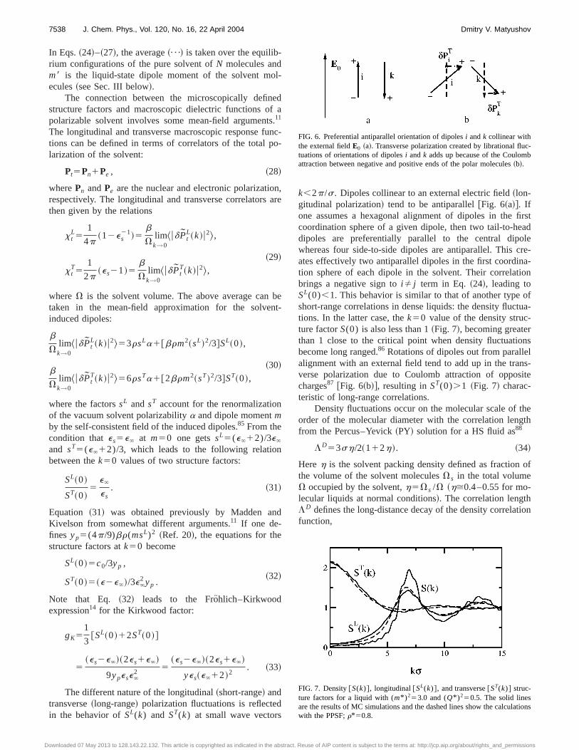
k,2p/s. Dipoles collinear to an external electric field~lon-gitudinal polarization! tend to be antiparallel@Fig. 6~a!#. Ifone assumes a hexagonal alignment of dipoles in the firstcoordination sphere of a given dipole, then two tail-to-headdipoles are preferentially parallel to the central dipolewhereas four side-to-side dipoles are antiparallel. This cre-ates effectively two antiparallel dipoles in the first coordina-tion sphere of each dipole in the solvent. Their correlationbrings a negative sign toiÞ j term in Eq. ~24!, leading toSL(0),1. This behavior is similar to that of another type ofshort-range correlations in dense liquids: the density fluctua-tions. In the latter case, thek50 value of the density struc-ture factorS(0) is also less than 1~Fig. 7!, becoming greaterthan 1 close to the critical point when density fluctuationsbecome long ranged.86 Rotations of dipoles out from parallelalignment with an external field tend to add up in the trans-verse polarization due to Coulomb attraction of oppositecharges87 @Fig. 6~b!#, resulting inST(0).1 ~Fig. 7! charac-teristic of long-range correlations.

Density fluctuations occur on the molecular scale of theorder of the molecular diameter with the correlation lengthfrom the Percus–Yevick~PY! solution for a HS fluid as88

LD53sh/2~112h!. ~34!

Hereh is the solvent packing density defined as fraction ofthe volume of the solvent moleculesVs in the total volumeV occupied by the solvent,h5Vs /V ~h>0.4–0.55 for mo-lecular liquids at normal conditions!. The correlation lengthLD defines the long-distance decay of the density correlationfunction,

FIG. 6. Preferential antiparallel orientation of dipolesi andk collinear withthe external fieldE0 ~a!. Transverse polarization created by librational fluc-tuations of orientations of dipolesi andk adds up because of the Coulombattraction between negative and positive ends of the polar molecules~b!.

FIG. 7. Density@S(k)#, longitudinal@SL(k)#, and transverse@ST(k)# struc-ture factors for a liquid with (m* )253.0 and (Q* )250.5. The solid linesare the results of MC simulations and the dashed lines show the calculationswith the PPSF;r*50.8.



^dr~r !dr~0!&}r 21e2r /LD. ~35!

Both the long-distance and short-distance behavior of thedensity correlations are described by the density structurefactor

S~k!511rhss000~k! ~36!

in which hss000(k) stands for the spherically symmetric com-

ponent of the solvent–solvent~subscript ‘‘ss’’ ! pair correla-tion function.45

C. Polarity dependence

The Marcus approximate relation forls employs thelongitudinal field of the ET dipole~transverse component isneglected! in the form

DE0L~k!5

4p ie

k@ j 0~kRD!2 j 0~kRA!eik"R#, ~37!

whereRD and RA are the radii of the spherical donor andacceptor units, respectively,R is the D–A distance, ande isthe elementary charge;j n(x) is the spherical Bessel functionof ordern. The substitution of Eq.~37! into Eqs.~1! and~2!leads to the relation

lsM5

e2c0

2 S 1

RD1

1

RA2

2

RD , ~38!

with lsM proportional to the Pekar factorc0 @Eq. ~1!#. Al-

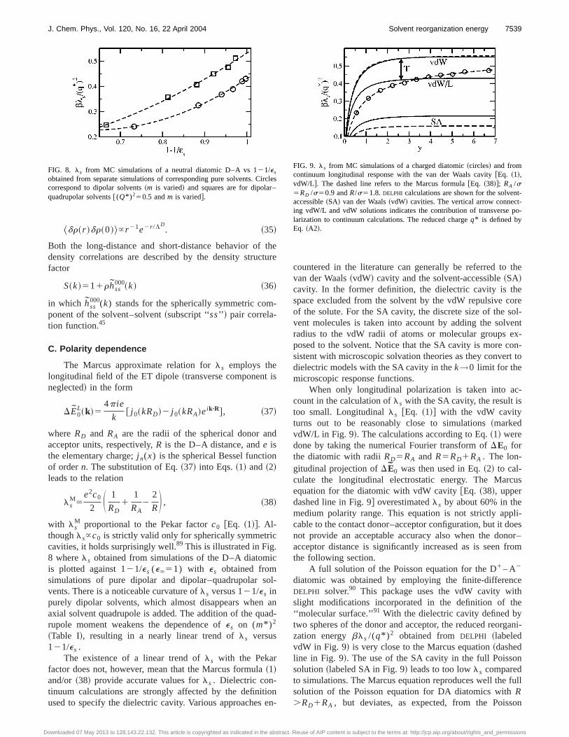
thoughls}c0 is strictly valid only for spherically symmetriccavities, it holds surprisingly well.89 This is illustrated in Fig.8 wherels obtained from simulations of the D–A diatomicis plotted against 121/es (e`51) with es obtained fromsimulations of pure dipolar and dipolar–quadrupolar sol-vents. There is a noticeable curvature ofls versus 121/es inpurely dipolar solvents, which almost disappears when anaxial solvent quadrupole is added. The addition of the quad-rupole moment weakens the dependence ofes on (m* )2

~Table I!, resulting in a nearly linear trend ofls versus121/es .

The existence of a linear trend ofls with the Pekarfactor does not, however, mean that the Marcus formula~1!and/or ~38! provide accurate values forls . Dielectric con-tinuum calculations are strongly affected by the definitionused to specify the dielectric cavity. Various approaches en-

countered in the literature can generally be referred to thevan der Waals~vdW! cavity and the solvent-accessible~SA!cavity. In the former definition, the dielectric cavity is thespace excluded from the solvent by the vdW repulsive coreof the solute. For the SA cavity, the discrete size of the sol-vent molecules is taken into account by adding the solventradius to the vdW radii of atoms or molecular groups ex-posed to the solvent. Notice that the SA cavity is more con-sistent with microscopic solvation theories as they convert todielectric models with the SA cavity in thek→0 limit for themicroscopic response functions.

When only longitudinal polarization is taken into ac-count in the calculation ofls with the SA cavity, the result istoo small. Longitudinalls @Eq. ~1!# with the vdW cavityturns out to be reasonably close to simulations~markedvdW/L in Fig. 9!. The calculations according to Eq.~1! weredone by taking the numerical Fourier transform ofDE0 forthe diatomic with radiiRD5RA and R5RD1RA . The lon-gitudinal projection ofDE0 was then used in Eq.~2! to cal-culate the longitudinal electrostatic energy. The Marcusequation for the diatomic with vdW cavity@Eq. ~38!, upperdashed line in Fig. 9# overestimatedls by about 60% in themedium polarity range. This equation is not strictly appli-cable to the contact donor–acceptor configuration, but it doesnot provide an acceptable accuracy also when the donor–acceptor distance is significantly increased as is seen fromthe following section.

A full solution of the Poisson equation for the D1 – A2

diatomic was obtained by employing the finite-differenceDELPHI solver.90 This package uses the vdW cavity withslight modifications incorporated in the definition of the‘‘molecular surface.’’91 With the dielectric cavity defined bytwo spheres of the donor and acceptor, the reduced reorgani-zation energybls /(q* )2 obtained fromDELPHI ~labeledvdW in Fig. 9! is very close to the Marcus equation~dashedline in Fig. 9!. The use of the SA cavity in the full Poissonsolution~labeled SA in Fig. 9! leads to too lowls comparedto simulations. The Marcus equation reproduces well the fullsolution of the Poisson equation for DA diatomics withR.RD1RA , but deviates, as expected, from the Poisson

FIG. 8. ls from MC simulations of a neutral diatomic D–A vs 121/es

obtained from separate simulations of corresponding pure solvents. Circlescorrespond to dipolar solvents~m is varied! and squares are for dipolar–quadrupolar solvents@(Q* )250.5 andm is varied#.

FIG. 9. ls from MC simulations of a charged diatomic~circles! and fromcontinuum longitudinal response with the van der Waals cavity@Eq. ~1!,vdW/L#. The dashed line refers to the Marcus formula@Eq. ~38!#; RA /s5RD /s50.9 andR/s51.8. DELPHI calculations are shown for the solvent-accessible~SA! van der Waals~vdW! cavities. The vertical arrow connect-ing vdW/L and vdW solutions indicates the contribution of transverse po-larization to continuum calculations. The reduced chargeq* is defined byEq. ~A2!.



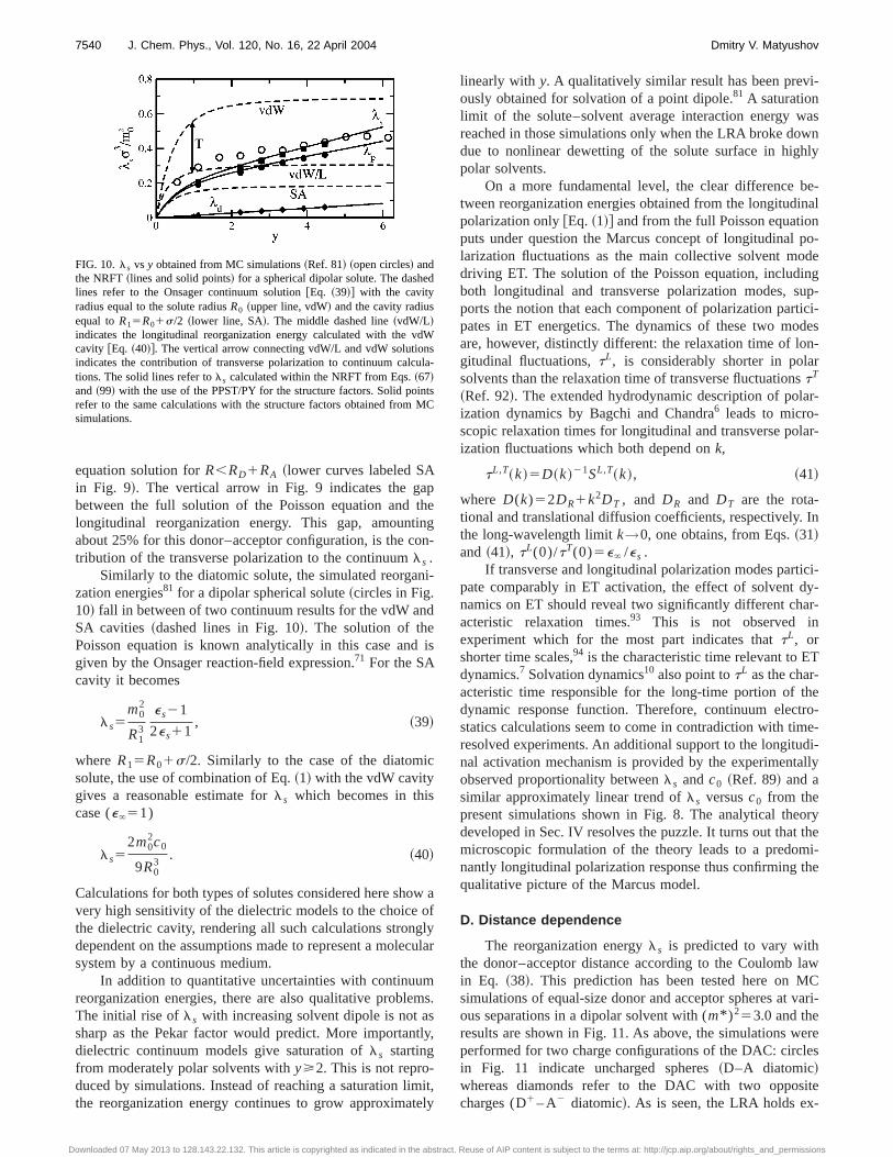
equation solution forR,RD1RA ~lower curves labeled SAin Fig. 9!. The vertical arrow in Fig. 9 indicates the gapbetween the full solution of the Poisson equation and thelongitudinal reorganization energy. This gap, amountingabout 25% for this donor–acceptor configuration, is the con-tribution of the transverse polarization to the continuumls .

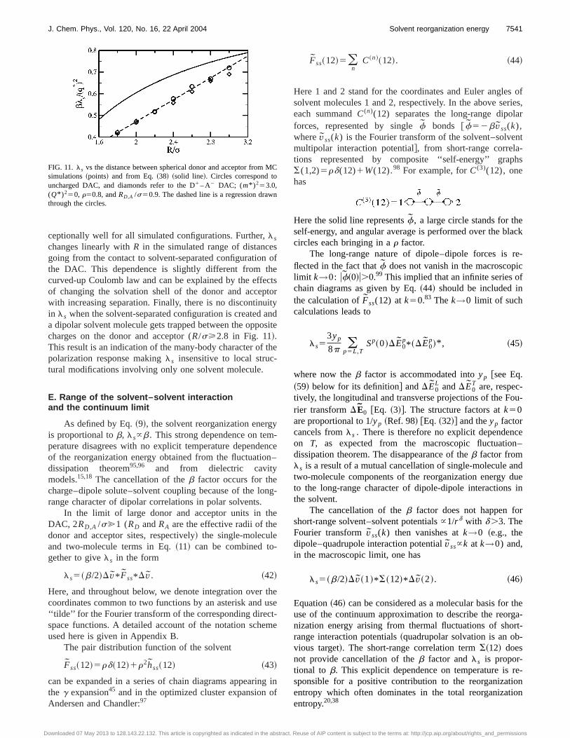
Similarly to the diatomic solute, the simulated reorgani-zation energies81 for a dipolar spherical solute~circles in Fig.10! fall in between of two continuum results for the vdW andSA cavities ~dashed lines in Fig. 10!. The solution of thePoisson equation is known analytically in this case and isgiven by the Onsager reaction-field expression.71 For the SAcavity it becomes

ls5m0

2

R13

es21

2es11, ~39!

where R15R01s/2. Similarly to the case of the diatomicsolute, the use of combination of Eq.~1! with the vdW cavitygives a reasonable estimate forls which becomes in thiscase (e`51)

ls52m0

2c0

9R03

. ~40!

Calculations for both types of solutes considered here show avery high sensitivity of the dielectric models to the choice ofthe dielectric cavity, rendering all such calculations stronglydependent on the assumptions made to represent a molecularsystem by a continuous medium.

In addition to quantitative uncertainties with continuumreorganization energies, there are also qualitative problems.The initial rise ofls with increasing solvent dipole is not assharp as the Pekar factor would predict. More importantly,dielectric continuum models give saturation ofls startingfrom moderately polar solvents withy>2. This is not repro-duced by simulations. Instead of reaching a saturation limit,the reorganization energy continues to grow approximately

linearly with y. A qualitatively similar result has been previ-ously obtained for solvation of a point dipole.81 A saturationlimit of the solute–solvent average interaction energy wasreached in those simulations only when the LRA broke downdue to nonlinear dewetting of the solute surface in highlypolar solvents.

On a more fundamental level, the clear difference be-tween reorganization energies obtained from the longitudinalpolarization only@Eq. ~1!# and from the full Poisson equationputs under question the Marcus concept of longitudinal po-larization fluctuations as the main collective solvent modedriving ET. The solution of the Poisson equation, includingboth longitudinal and transverse polarization modes, sup-ports the notion that each component of polarization partici-pates in ET energetics. The dynamics of these two modesare, however, distinctly different: the relaxation time of lon-gitudinal fluctuations,tL, is considerably shorter in polarsolvents than the relaxation time of transverse fluctuationstT

~Ref. 92!. The extended hydrodynamic description of polar-ization dynamics by Bagchi and Chandra6 leads to micro-scopic relaxation times for longitudinal and transverse polar-ization fluctuations which both depend onk,

tL,T~k!5D~k!21SL,T~k!, ~41!

where D(k)52DR1k2DT , and DR and DT are the rota-tional and translational diffusion coefficients, respectively. Inthe long-wavelength limitk→0, one obtains, from Eqs.~31!and ~41!, tL(0)/tT(0)5e` /es .

If transverse and longitudinal polarization modes partici-pate comparably in ET activation, the effect of solvent dy-namics on ET should reveal two significantly different char-acteristic relaxation times.93 This is not observed inexperiment which for the most part indicates thattL, orshorter time scales,94 is the characteristic time relevant to ETdynamics.7 Solvation dynamics10 also point totL as the char-acteristic time responsible for the long-time portion of thedynamic response function. Therefore, continuum electro-statics calculations seem to come in contradiction with time-resolved experiments. An additional support to the longitudi-nal activation mechanism is provided by the experimentallyobserved proportionality betweenls andc0 ~Ref. 89! and asimilar approximately linear trend ofls versusc0 from thepresent simulations shown in Fig. 8. The analytical theorydeveloped in Sec. IV resolves the puzzle. It turns out that themicroscopic formulation of the theory leads to a predomi-nantly longitudinal polarization response thus confirming thequalitative picture of the Marcus model.

D. Distance dependence

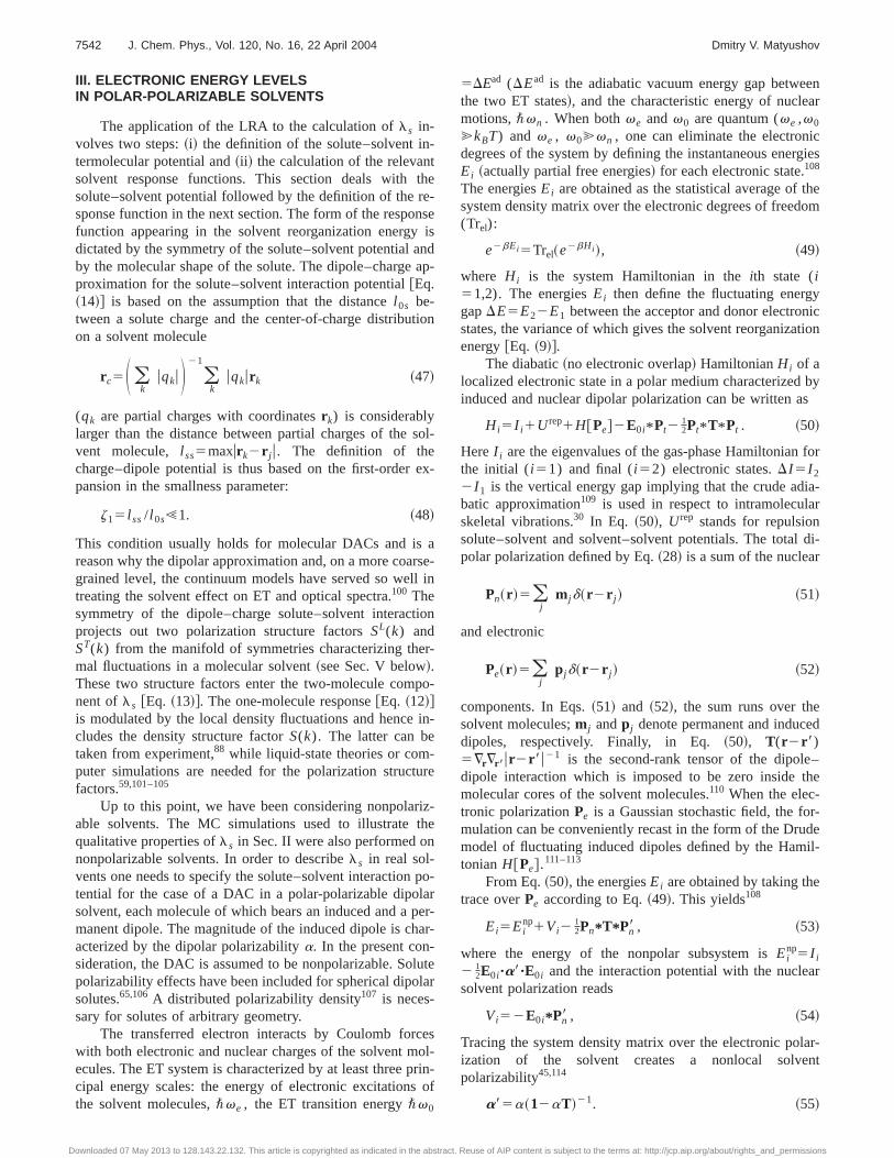
The reorganization energyls is predicted to vary withthe donor–acceptor distance according to the Coulomb lawin Eq. ~38!. This prediction has been tested here on MCsimulations of equal-size donor and acceptor spheres at vari-ous separations in a dipolar solvent with (m* )253.0 and theresults are shown in Fig. 11. As above, the simulations wereperformed for two charge configurations of the DAC: circlesin Fig. 11 indicate uncharged spheres~D–A diatomic!whereas diamonds refer to the DAC with two oppositecharges (D1 – A2 diatomic!. As is seen, the LRA holds ex-

FIG. 10. ls vs y obtained from MC simulations~Ref. 81! ~open circles! andthe NRFT~lines and solid points! for a spherical dipolar solute. The dashedlines refer to the Onsager continuum solution@Eq. ~39!# with the cavityradius equal to the solute radiusR0 ~upper line, vdW! and the cavity radiusequal toR15R01s/2 ~lower line, SA!. The middle dashed line~vdW/L!indicates the longitudinal reorganization energy calculated with the vdWcavity @Eq. ~40!#. The vertical arrow connecting vdW/L and vdW solutionsindicates the contribution of transverse polarization to continuum calcula-tions. The solid lines refer tols calculated within the NRFT from Eqs.~67!and~99! with the use of the PPST/PY for the structure factors. Solid pointsrefer to the same calculations with the structure factors obtained from MCsimulations.



ceptionally well for all simulated configurations. Further,ls

changes linearly withR in the simulated range of distancesgoing from the contact to solvent-separated configuration ofthe DAC. This dependence is slightly different from thecurved-up Coulomb law and can be explained by the effectsof changing the solvation shell of the donor and acceptorwith increasing separation. Finally, there is no discontinuityin ls when the solvent-separated configuration is created anda dipolar solvent molecule gets trapped between the oppositecharges on the donor and acceptor (R/s>2.8 in Fig. 11!.This result is an indication of the many-body character of thepolarization response makingls insensitive to local struc-tural modifications involving only one solvent molecule.

E. Range of the solvent–solvent interactionand the continuum limit

As defined by Eq.~9!, the solvent reorganization energyis proportional tob, ls}b. This strong dependence on tem-perature disagrees with no explicit temperature dependenceof the reorganization energy obtained from the fluctuation–dissipation theorem95,96 and from dielectric cavitymodels.15,18 The cancellation of theb factor occurs for thecharge–dipole solute–solvent coupling because of the long-range character of dipolar correlations in polar solvents.

In the limit of large donor and acceptor units in theDAC, 2RD,A /s@1 (RD andRA are the effective radii of thedonor and acceptor sites, respectively! the single-moleculeand two-molecule terms in Eq.~11! can be combined to-gether to givels in the form

ls5~b/2!D v* Fss* D v. ~42!

Here, and throughout below, we denote integration over thecoordinates common to two functions by an asterisk and use‘‘tilde’’ for the Fourier transform of the corresponding direct-space functions. A detailed account of the notation schemeused here is given in Appendix B.

The pair distribution function of the solvent

Fss~12!5rd~12!1r2hss~12! ~43!

can be expanded in a series of chain diagrams appearing inthe g expansion45 and in the optimized cluster expansion ofAndersen and Chandler:97

Fss~12!5(n

C~n!~12!. ~44!

Here 1 and 2 stand for the coordinates and Euler angles ofsolvent molecules 1 and 2, respectively. In the above series,each summandC(n)(12) separates the long-range dipolarforces, represented by singlef bonds @f52b vss(k),wherevss(k) is the Fourier transform of the solvent–solventmultipolar interaction potential#, from short-range correla-tions represented by composite ‘‘self-energy’’ graphsS(1,2)5rd(12)1W(12).98 For example, forC(3)(12), onehas

Here the solid line representsf, a large circle stands for theself-energy, and angular average is performed over the blackcircles each bringing in ar factor.

The long-range nature of dipole–dipole forces is re-flected in the fact thatf does not vanish in the macroscopiclimit k→0: uf~0!u.0.99 This implied that an infinite series ofchain diagrams as given by Eq.~44! should be included inthe calculation ofFss(12) atk50.83 The k→0 limit of suchcalculations leads to

ls53yp

8p (p5L,T

Sp~0!DE0p* ~DE0

p!* , ~45!

where now theb factor is accommodated intoyp @see Eq.~59! below for its definition# andDE0

L andDE0T are, respec-

tively, the longitudinal and transverse projections of the Fou-rier transformDE0 @Eq. ~3!#. The structure factors atk50are proportional to 1/yp ~Ref. 98! @Eq. ~32!# and theyp factorcancels fromls . There is therefore no explicit dependenceon T, as expected from the macroscopic fluctuation–dissipation theorem. The disappearance of theb factor fromls is a result of a mutual cancellation of single-molecule andtwo-molecule components of the reorganization energy dueto the long-range character of dipole-dipole interactions inthe solvent.

The cancellation of theb factor does not happen forshort-range solvent–solvent potentials}1/r d with d .3. TheFourier transformvss(k) then vanishes atk→0 ~e.g., thedipole–quadrupole interaction potentialvss}k at k→0) and,in the macroscopic limit, one has

ls5~b/2!D v~1!* S~12!* D v~2!. ~46!

Equation~46! can be considered as a molecular basis for theuse of the continuum approximation to describe the reorga-nization energy arising from thermal fluctuations of short-range interaction potentials~quadrupolar solvation is an ob-vious target!. The short-range correlation termS~12! doesnot provide cancellation of theb factor andls is propor-tional to b. This explicit dependence on temperature is re-sponsible for a positive contribution to the reorganizationentropy which often dominates in the total reorganizationentropy.20,38

FIG. 11. ls vs the distance between spherical donor and acceptor from MCsimulations~points! and from Eq.~38! ~solid line!. Circles correspond touncharged DAC, and diamonds refer to the D1 – A2 DAC; (m* )253.0,(Q* )250, r50.8, andRD,A /s50.9. The dashed line is a regression drawnthrough the circles.



III. ELECTRONIC ENERGY LEVELSIN POLAR-POLARIZABLE SOLVENTS

The application of the LRA to the calculation ofls in-volves two steps:~i! the definition of the solute–solvent in-termolecular potential and~ii ! the calculation of the relevantsolvent response functions. This section deals with thesolute–solvent potential followed by the definition of the re-sponse function in the next section. The form of the responsefunction appearing in the solvent reorganization energy isdictated by the symmetry of the solute–solvent potential andby the molecular shape of the solute. The dipole–charge ap-proximation for the solute–solvent interaction potential@Eq.~14!# is based on the assumption that the distancel 0s be-tween a solute charge and the center-of-charge distributionon a solvent molecule

r c5S (k

uqku D 21

(k

uqkur k ~47!

(qk are partial charges with coordinatesr k) is considerablylarger than the distance between partial charges of the sol-vent molecule, l ss5maxur k2r j u. The definition of thecharge–dipole potential is thus based on the first-order ex-pansion in the smallness parameter:

z15 l ss/ l 0s!1. ~48!

This condition usually holds for molecular DACs and is areason why the dipolar approximation and, on a more coarse-grained level, the continuum models have served so well intreating the solvent effect on ET and optical spectra.100 Thesymmetry of the dipole–charge solute–solvent interactionprojects out two polarization structure factorsSL(k) andST(k) from the manifold of symmetries characterizing ther-mal fluctuations in a molecular solvent~see Sec. V below!.These two structure factors enter the two-molecule compo-nent ofls @Eq. ~13!#. The one-molecule response@Eq. ~12!#is modulated by the local density fluctuations and hence in-cludes the density structure factorS(k). The latter can betaken from experiment,88 while liquid-state theories or com-puter simulations are needed for the polarization structurefactors.59,101–105

Up to this point, we have been considering nonpolariz-able solvents. The MC simulations used to illustrate thequalitative properties ofls in Sec. II were also performed onnonpolarizable solvents. In order to describels in real sol-vents one needs to specify the solute–solvent interaction po-tential for the case of a DAC in a polar-polarizable dipolarsolvent, each molecule of which bears an induced and a per-manent dipole. The magnitude of the induced dipole is char-acterized by the dipolar polarizabilitya. In the present con-sideration, the DAC is assumed to be nonpolarizable. Solutepolarizability effects have been included for spherical dipolarsolutes.65,106A distributed polarizability density107 is neces-sary for solutes of arbitrary geometry.

The transferred electron interacts by Coulomb forceswith both electronic and nuclear charges of the solvent mol-ecules. The ET system is characterized by at least three prin-cipal energy scales: the energy of electronic excitations ofthe solvent molecules,\ve , the ET transition energy\v0

5DEad (DEad is the adiabatic vacuum energy gap betweenthe two ET states!, and the characteristic energy of nuclearmotions,\vn . When bothve andv0 are quantum (ve ,v0

@kBT) and ve , v0@vn , one can eliminate the electronicdegrees of the system by defining the instantaneous energiesEi ~actually partial free energies! for each electronic state.108

The energiesEi are obtained as the statistical average of thesystem density matrix over the electronic degrees of freedom(Trel):

e2bEi5Trel~e2bHi !, ~49!

where Hi is the system Hamiltonian in theith state (i51,2). The energiesEi then define the fluctuating energygapDE5E22E1 between the acceptor and donor electronicstates, the variance of which gives the solvent reorganizationenergy@Eq. ~9!#.

The diabatic~no electronic overlap! HamiltonianHi of alocalized electronic state in a polar medium characterized byinduced and nuclear dipolar polarization can be written as

Hi5I i1U rep1H@Pe#2E0i* Pt212Pt* T* Pt . ~50!

HereI i are the eigenvalues of the gas-phase Hamiltonian forthe initial (i 51) and final (i 52) electronic states.DI 5I 2

2I 1 is the vertical energy gap implying that the crude adia-batic approximation109 is used in respect to intramolecularskeletal vibrations.30 In Eq. ~50!, U rep stands for repulsionsolute–solvent and solvent–solvent potentials. The total di-polar polarization defined by Eq.~28! is a sum of the nuclear

Pn~r !5(j

mjd~r2r j ! ~51!

and electronic

Pe~r !5(j

pjd~r2r j ! ~52!

components. In Eqs.~51! and ~52!, the sum runs over thesolvent molecules;mj andpj denote permanent and induceddipoles, respectively. Finally, in Eq.~50!, T(r2r 8)5¹r¹r8ur2r 8u21 is the second-rank tensor of the dipole–dipole interaction which is imposed to be zero inside themolecular cores of the solvent molecules.110 When the elec-tronic polarizationPe is a Gaussian stochastic field, the for-mulation can be conveniently recast in the form of the Drudemodel of fluctuating induced dipoles defined by the Hamil-tonianH@Pe#.

111–113

From Eq.~50!, the energiesEi are obtained by taking thetrace overPe according to Eq.~49!. This yields108

Ei5Einp1Vi2

12Pn*T*Pn8 , ~53!

where the energy of the nonpolar subsystem isEinp5I i

2 12E0i "a8"E0i and the interaction potential with the nuclear

solvent polarization reads

Vi52E0i*Pn8 , ~54!

Tracing the system density matrix over the electronic polar-ization of the solvent creates a nonlocal solventpolarizability45,114

a85a~12aT!21. ~55!



In addition, the nuclear polarization is renormalized to114

Pn85~12aT!21•Pn . ~56!

This renormalization accounts for the well-known enhance-ment of the solvent permanent dipoles by the electric field ofthe induced solvent dipoles.45 Note that neitherPn nor Pn8 isassumed to be a continuous polarization density used in con-tinuum dielectric models. From the definition in Eq.~51!, Ei

can be rewritten as

Ei5Einp1U rep2(

jE0i "mj82 1

2 (j Þk

mj "T jk"mk8 , ~57!

whereT jk5T(r j2r k) and

mj85(k

~12aT! jk21"mk ~58!

is the effective condensed-phase solvent dipole. The corre-sponding microscopic dimensionless density of permanentdipoles is

yp5~4p/9!br~m8!2. ~59!

Equation~55! shows that, after tracing the induced solventdipoles, the pure solvent is described by the Hamiltonian of adipolar nonpolarizable solvent with the effective permanentdipoles (mm8)1/2. An external field, however, interacts withm8 and this is the reason whym8 and not (mm8)1/2 appearsin the equations related to dielectric properties of the solventobtained as linear response to an external electric field.45

IV. SOLVENT REORGANIZATION ENERGY

The formalism of nonlocal response functions developedhere aims at expressingls in terms of the molecular shape ofthe solute and parameters characteristic of the pure solvent.The solvent thermal motions are projected onto two solventstructure factors: the density structure factor and the dipolarpolarization structure factor. The latter is split into its longi-tudinal and transverse components, reflecting the anisotropyof the dipole–dipole interactions.

The free energy surfaces of ET,Fi(X), can be repre-sented by a Fourier integral of the generating functionalGi(z):

e2bFi ~X!5E2`

` dz

2pei z~X2DEnp!Gi~z!, ~60!

where X is the energy gap reaction coordinate,DEnp5E2np

2E1np, and

Gi~z!5QB21Tr@e~ i zDE01bE0i !*Pn82bUrep2bHB#. ~61!

HereQB5Tr(exp@2bHB#) andHB describes the nuclear sub-system of the pure solvent~thermal bath!.

The generating functional can be expanded in Mayerfunctions defined on the solute–solvent interactionpotential.20,32 The exact result of this expansion is

ln Gi~z!5rE f i~1,z!dG1

1~r2/2!E f i~1,z! f i~2,z!hss~12!dG1dG21~r3/6!

3E f i~1,z! f i~2,z! f i~3,z!hss~123!dG1dG2dG3

1¯, ~62!

with

f i~1,z!5em18•@ i zDE~r1!1bE0i !2bUrep~r1!21 ~63!

andhss(12) andhss(123) standing for, respectively, the pairand three-particle correlation functions of the pure solvent.

The Gaussian~LRA! approximation follows from Eq.~62! by expanding the Mayer functions in powers ofz andtruncating the expansion after the second order. The result ofthis procedure is the solvent reorganization energy given as asum of two components:20,32

ls5lp1ld . ~64!

The first component reflects the energetic strength of aniso-tropic fluctuations of the solvent polarization~orientationalreorganization energy20!:

lp5 12 DE0* x* DE0* , ~65!

where the asterisk inDE0* stands for complex conjugate. Thepolarization response function is defined on the polarizationstructure factors

x~k12k2!5dk1 ,k2xs~k2!,

~66!

xs~k!53yp

4p@SL~k!JL1ST~k!JT#,

where JL5 kk, JT512 kk, yp is given by Eq.~59!, anddk1 ,k2

5(2p)3d(k12k2). The orientational reorganizationenergy in Eq.~65! is given in terms of the response of thepure solvent restricted to the volume outside the DAC.

The componentld in Eq. ~64! describes the alteration ofthe solvent response by the local density profile of the sol-vent around the solute. It is built on the density structurefactor and is called the density reorganization energy.20,32 Ifthree-molecule and all higher-order correlation functions aredropped from Eq.~62!, the componentld becomes32

ld523yp

8pDE0* ~S21!u0* DE0* , ~67!

where the kernelu0(k12k2) projects the response inside thesolute volumeV0 :

u0~k12k2!5EV0

ei ~k12k2!"rdr . ~68!

Note thatV0 is the space inaccessible to the solvent—i.e., aregion surrounded by the SA surface~Sec. II C!.



There is a mathematical and physical similarity betweenthe reorganization components arising from orientational anddensity correlations. In order to make it clear we rewrite Eqs.~64!–~67! as

ls53ypE013yp

8p (p5L,T

DE0p* ~Sp21!* ~DE0

p!*

23yp

8pDE0* ~S21!u0* DE0* . ~69!

The first term in Eq.~69! is the electrostatic energy of the ETdipole in a uniform medium outside the solute characterizedby the dipolar densityyp :

E05~8p!21EV

DE0~r !2dr

5~8p!21 (p5L,T

DE0p* ~DE0

p!* . ~70!

This term arises from the one-particle responsel I represent-ing changes in orientations and positions of a single solventmolecule not hindered by the restoring field of its neighbors.In a dense liquid solvent, molecular motions are affected bythe restoring electric field of the surrounding molecules andby their repulsive cores. These two effects are represented bythe second and third summands in Eq.~69!, respectively. Asdiscussed in Sec. II A, strong orientational correlationsamong the solvent dipoles cancel almost completely the elec-trostatic energy term 3ypE0 . The density correlations aremore short ranged and give a smaller contribution tols .They are, however, significant for the reorganization entropydue to an explicit 1/T temperature dependence~Sec.II E!.20,32 The density reorganization term disappears in thelimit of a macroscopic solute when only the orientationalcomponent is significant,ls5lp , and the reorganization en-ergy tends to its continuum limit given by Eq.~45! ~see Sec.VI C for the criterion of applicability of continuum models!.

Equations~45! and ~69! highlight problems arising withsimple perturbation~and Mayer function! formulations forlp . If the difference field has only a longitudinal component,as in the Marcus formulation in Eqs.~1! and ~37!, Eq. ~45!transforms into Eq.~1!. When DE0

T is nonzero, the con-tinuum estimate of the transverse reorganization term@Eq.~45!#

lsT5~es21!E0

T ~71!

rises linearly with the solvent dielectric constant. The trans-verse electrostatic energy

E0T5~8p!21E dk

~2p!3uDE0

Tu2 ~72!

is often small compared toE0L for common ET systems.

However, the factor (es21) in Eq. ~71! makeslsT grow

strongly with increasing solvent polarity. This is not seen inMC simulations. Although simulations do not show satura-tion of ls predicted by the dielectric continuum models~Fig.9!, the growth ofls with solvent polarity is obviously slowerthan would appear fromls

T in Eq. ~71!. At largees the term

lT results in the ‘‘transverse catastrophe’’ ofls divergingwith increasinges . The flaw of Eq.~65! is that it does notincorporate the alteration of the polarization response by theinsertion of the solute. The perturbation created by excludingpolarization from the solute’s volume propagates over a mac-roscopic distance due to the long-range length scale of trans-verse polarization fluctuations. This effect alters the con-tinuum response function as is commonly accommodatedinto dielectric theories through cavity boundary conditions.Chandler’s Gaussian model was designed to include this al-teration of the response function on the microscopic lengthscale.54–56Below, we adopt this approach to reformulate theexpression forlp .

In the Gaussian model, the generating functional is ob-tained through functional integration over the nuclear polar-ization field:55,56

G~z!5~QB!21E ei zDE0* Pn82bHB)V0

d@Pn8~r !#DPn8 . ~73!

Since the LRA holds for ET reorganization, it is sufficient tocalculate the response function atE0i50 and, therefore, theinteraction of the solute with the solvent is dropped from thestatistical average@cf. Eqs. ~61! and ~73!#. In Eq. ~73!, theproductPV0

is over the space points inside the solute thusexcluding the solvent polarization from the solute volume.115

The bath HamiltonianHB describes Gaussian fluctuations ofthe polarization field weighted with the polarization correla-tion function:

HB5 12 Pn8* x21* ~Pn8!* . ~74!

The functional integration in Eq.~73! leads to the orien-tational reorganization energy still defined by Eq.~65! withthe polarization response function changed fromx to a modi-fied response functionxm given by the equation54

xm5x2x* u0* G21* u0* x. ~75!

Here the kernelG21(k1 ,k2) is the inverse of

G~k1 ,k2!5u0~k12k8!* x~k82k9!* u0~k92k2!. ~76!

The kernelG can be rewritten in the form

G~k1 ,k2!5u0~k12k2!@xs~k2!2x8~k2!#, ~77!

where

x8~k2!5EV8

drE ei ~k2k2!•rxs~k!dk

~2p!3. ~78!

Here the regionV8 is outside the regionV08 made by thespace pointsr12r2 with r1,2 belonging toV0 .

Equation~75! is changed from the original formulationof the Gaussian model54–56 in which the functionxm acts onthe solute field not modified by the cutoff volumeV0 . In-stead, when Eq.~75! is used in Eq.~65! the response func-tion acts on the solute field defined outside the DAC@Eq.~3!#. This transformation is achieved in terms of projections



of the response ‘‘in’’ and ‘‘out’’ of the DAC. The projectioninside the DAC is defined byu0 in Eq. ~68! while the pro-jection outside the DAC is given by

u~k12k2!5EV

e~k12k2!"rdr . ~79!

The kernelsu0 andu satisfy the usual algebra of projectionoperators:

u01u51,

u0* u50,~80!

u0* u05u0 ,

u* u5u,

where1 in Eq. ~80! stands fordk1 ,k2.

The substitution of Eqs.~77! and~78! into Eq.~75! leadsto the response function

xm~k1 ,k2!5xs~k1!dk1 ,k22x9~k1!u0~k12k2!xs~k2!,

~81!

wherex95x"@x2x8#21 can be expressed through the lon-gitudinal and transverse components ofx8 as

x95JLSL

SL2x8L1JT

ST

ST2x8T. ~82!

Equations~81! and~82! give an exact solution for the renor-malization of orientational polarization response in the pres-ence of a solute of arbitrary form. From Eq.~81! the reorga-nization energylp can be rewritten as

lp5lL1lT2lcorr, ~83!

where

lL,T53yp

8puDE0

L,Tu2* SL,T. ~84!

The correction termlcorr accounts for the modification of thepolarization response by the presence of the solute. It can bewritten in the form avoiding the convolution in the invertedspace as follows:

lcorr53yp

8p EV0

DE08~r !•DE09~r !dr , ~85!

where the new effective fieldsDE08 andDE09 are the inverseFourier transforms of the expressions

DE08~k!5 kDE0L~k!~SL~k!2ST~k!!1DE0~k!ST~k!

~86!

and

DE09~k!5 kDE0L~k!@~x9!L~k!2~x9!T~k!#

1DE0~k!~x9!T~k!. ~87!

The main challenge in practical applications of thepresent formalism is the calculation of the functionx8. Weprovide here an approximate derivation applicable to soluteswhich are large compared to the solvent molecules. The in-tegration overk in Eq. ~78! yields

x8~k!5EV8

dr eik"rF S d~r !1r

3h110~r ! D1

1r

3h112~r !DrG , ~88!

with Dr53r r21. In the above integral, only the long-range112 component survives for large solutes. The asymptoticform of h112(r ) can be found from Eq.~32! as

rh112~r !.c0

2es

4pyp

1

r 3. ~89!

When Eq.~89! is used in Eq.~88!, one obtains

x8~k!5c0

2es

12pypE

V8

Dr

r 3eik"rdr . ~90!

This expression represents the Fourier transform of therank-2 tensor corresponding to a point dipole placed at thecenter of the cavity formed by the regionV08 . When thesolute is a spherical cavity of the radiusR1 the solution is

x8~k!522A~k!JL1A~k!JT, ~91!

with

A~k!5c0

2es

3yp

j 1~2kR1!

2kR1. ~92!

From Eq.~91! the functionx 9 in Eq. ~82! becomes

x 95JLSL

SL12A1JT

ST

ST2A. ~93!

At k50, SL(0)12A(0)5ST(0)2A(0)5gK @Eq. ~33!# andx 9 turns intogK

21xs in the continuum limit. The functionx 9from Eq.~93! can be used in Eq.~87! to obtain the correctionof solvent’s polarization response by solute’s repulsive core.Before turning to a general solution, we first consider a sim-pler case of a dipolar spherical solute for which an exactanalytical solution is possible.116

A. Dipolar solute

An exact solution forlp can be obtained for a pointdipole approximation for the field of ET dipole. When, inaddition, the solute is represented by a sphere of an effectiveradiusR0 , DE0 is given by the relation

DE0~k!524pm0"Dk

j 1~kR1!

kR1, ~94!

whereDk53kk21 andm0 is the ET dipole moment. FromEqs.~87! and~93! the fieldDE09 is the inverse Fourier trans-form given as

DE09~r !5E dk

~2p!3@S1kDE0

L1S2DE0#e2 ik"r, ~95!

where

S15SL

SL12A2

ST

ST2A, ~96!



S25ST

ST2A.

Since the space integral inlcorr @Eq. ~85!# is taken over thesolute volume, one needs to calculate the above integral forr<R1 only. The integral is calculated by complexk-planeintegration. The functionsSL/(SL12A) andST/(ST2A) donot have singularities in the complexk plane since existingsingularities of SL,T cancel out in the nominator anddenominator.117 Therefore, only thek50 pole of DE0 con-tributes to the integral. The result of integration within thesolute sphere,r ,R1 is then a constant field:116

DE0952m0

3gKR13 @ST~0!2SL~0!#. ~97!

This result greatly simplifies the solution forlcorr, whichbecomes

lcorr5ST~0!2SL~0!

3gK@2lT2lL#. ~98!

From Eqs.~83! and ~98!, the reorganization energylp is

lp5gK21ST~0!lL1gK

21SL~0!lT. ~99!

WhenlL andlT @Eq. ~84!# are calculated in the continuumlimit by assumingSL,T(k)5SL,T(0) one arrives at the solu-tion

lp5m0

2

R13

es2e`

e`2 ~2es1e`!

. ~100!

Equation~100! transforms into the Onsager form in Eq.~39!whene`51.

Equation~99! presents an exact solution forlp of ET inan arbitrary dielectric material characterized by longitudinaland transverse structure factors whenDE0 is approximatedby the point dipole field. The convergence of Eq.~99! intothe Onsager continuum limit indicates that the NRFT doesresolve the problem of a ‘‘transverse catastrophe’’ posed bydirect perturbation expansions.116 The continuum limit of theNRFT @Eq. ~100!# yields a significantly stronger dependenceof lp on e` than the one suggested by the Lippert–Mataga~superscript ‘‘LM’’! equation.100 The latter predicts thatlp isproportional to the polarity parameter

f pLM5

es21

2es112

e`21

2e`11. ~101!

Equation ~101! is based on the assumption that electronicand nuclear solvations additively contribute to the total sol-vation free energy. The numerical accuracy of this assump-tion is supported by MC simulations of dipolar solvation inpolarizable solvents.65 However, compared to both liquid-state theories and simulations, the Lippert–Mataga equationgreatly overestimates the falloff oflp with increasinge`

~Ref. 65!.The continuum limit of the NRFT allows us to draw two

conclusions. First, the additive approximation is not exact.Second, the continuumlp in Eq. ~100! depends morestrongly one` than the Lippert–Mataga equation suggests.

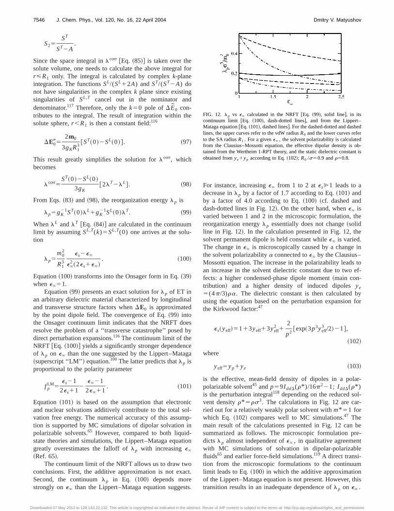
For instance, increasinge` from 1 to 2 ates@1 leads to adecrease inlp by a factor of 1.7 according to Eq.~101! andby a factor of 4.0 according to Eq.~100! ~cf. dashed anddash-dotted lines in Fig. 12!. On the other hand, whene` isvaried between 1 and 2 in the microscopic formulation, thereorganization energylp essentially does not change~solidline in Fig. 12!. In the calculation presented in Fig. 12, thesolvent permanent dipole is held constant whilee` is varied.The change ine` is microscopically caused by a change inthe solvent polarizabilitya connected toe` by the Clausius–Mossotti equation. The increase in the polarizability leads toan increase in the solvent dielectric constant due to two ef-fects: a higher condensed-phase dipole moment~main con-tribution! and a higher density of induced dipolesye

5(4p/3)ra. The dielectric constant is then calculated byusing the equation based on the perturbation expansion forthe Kirkwood factor:47

es~yeff!5113yeff13yeff2 1

2

p2@exp~3p3yeff

3 /2!21#,

~102!

where

yeff5yp1ye ~103!

is the effective, mean-field density of dipoles in a polar-polarizable solvent45 andp59I ddD(r* )/16p221; I ddD(r* )is the perturbation integral118 depending on the reduced sol-vent densityr* 5rs3. The calculations in Fig. 12 are car-ried out for a relatively weakly polar solvent withm* 51 forwhich Eq. ~102! compares well to MC simulations.47 Themain result of the calculations presented in Fig. 12 can besummarized as follows. The microscopic formulation pre-dicts lp almost independent ofe` , in qualitative agreementwith MC simulations of solvation in dipolar-polarizablefluids65 and earlier force-field simulations.119 A direct transi-tion from the microscopic formulations to the continuumlimit leads to Eq.~100! in which the additive approximationof the Lippert–Mataga equation is not present. However, thistransition results in an inadequate dependence oflp on e` .

FIG. 12. lp vs e` calculated in the NRFT@Eq. ~99!, solid line#, in itscontinuum limit @Eq. ~100!, dash-dotted lines#, and from the Lippert–Mataga equation@Eq. ~101!, dashed lines#. For the dashed-dotted and dashedlines, the upper curves refer to the vdW radiusR0 and the lower curves referto the SA radiusR1 . For a givene` , the solvent polarizability is calculatedfrom the Clausius–Mossotti equation, the effective dipolar density is ob-tained from the Wertheim 1-RPT theory, and the static dielectric constant isobtained fromye1yp according to Eq.~102!; R0 /s50.9 andr50.8.



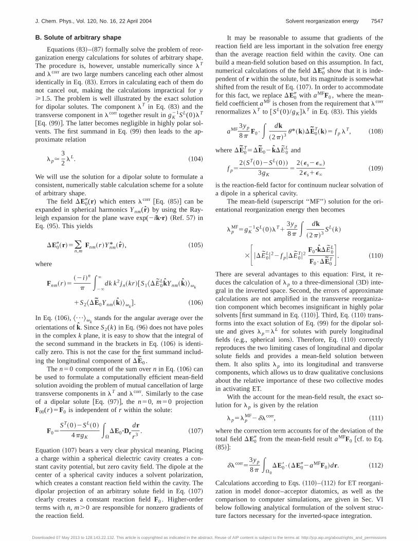
B. Solute of arbitrary shape

Equations~83!–~87! formally solve the problem of reor-ganization energy calculations for solutes of arbitrary shape.The procedure is, however, unstable numerically sincelT

andlcorr are two large numbers canceling each other almostidentically in Eq.~83!. Errors in calculating each of them donot cancel out, making the calculations impractical fory>1.5. The problem is well illustrated by the exact solutionfor dipolar solutes. The componentlT in Eq. ~83! and thetransverse component inlcorr together result ingK

21SL(0)lT

@Eq. ~99!#. The latter becomes negligible in highly polar sol-vents. The first summand in Eq.~99! then leads to the ap-proximate relation

lp.3

2lL. ~104!

We will use the solution for a dipolar solute to formulate aconsistent, numerically stable calculation scheme for a soluteof arbitrary shape.

The field DE09(r ) which enterslcorr @Eq. ~85!# can beexpanded in spherical harmonicsYnm( r ) by using the Ray-leigh expansion for the plane wave exp(2ik"r ) ~Ref. 57! inEq. ~95!. This yields

DE09~r !5(n,m

Fnm~r !Ynm* ~ r !, ~105!

where

Fnm~r !5~2 i !n

p E2`

`

dk k2 j n~kr !@S1^DE0LkYnm~ k!&vk

1S2^DE0Ynm~ k!&vk#. ~106!

In Eq. ~106!, ^¯&vkstands for the angular average over the

orientations ofk. SinceS2(k) in Eq. ~96! does not have polesin the complexk plane, it is easy to show that the integral ofthe second summand in the brackets in Eq.~106! is identi-cally zero. This is not the case for the first summand includ-ing the longitudinal component ofDE0 .

Then50 component of the sum overn in Eq. ~106! canbe used to formulate a computationally efficient mean-fieldsolution avoiding the problem of mutual cancellation of largetransverse components inlT andlcorr. Similarly to the caseof a dipolar solute@Eq. ~97!#, the n50, m50 projectionF00(r )5F0 is independent ofr within the solute:

F05ST~0!2SL~0!

4pgKE

VDE0"Dr

dr

r 3. ~107!

Equation~107! bears a very clear physical meaning. Placinga charge within a spherical dielectric cavity creates a con-stant cavity potential, but zero cavity field. The dipole at thecenter of a spherical cavity induces a solvent polarization,which creates a constant reaction field within the cavity. Thedipolar projection of an arbitrary solute field in Eq.~107!clearly creates a constant reaction fieldF0 . Higher-orderterms withn, m.0 are responsible for nonzero gradients ofthe reaction field.

It may be reasonable to assume that gradients of thereaction field are less important in the solvation free energythan the average reaction field within the cavity. One canbuild a mean-field solution based on this assumption. In fact,numerical calculations of the fieldDE09 show that it is inde-pendent ofr within the solute, but its magnitude is somewhatshifted from the result of Eq.~107!. In order to accommodatefor this fact, we replaceDE09 with aMFF0 , where the mean-field coefficientaMF is chosen from the requirement thatlcorr

renormalizeslT to @SL(0)/gK#lT in Eq. ~83!. This yields

aMF3yp

8pF0•E dk

~2p!3u* ~k!DE0

T~k!5 f p lT, ~108!

whereDE0T5DE02 kDE0

L and

f p52~ST~0!2SL~0!!

3gK5

2~es2e`!

2es1e`~109!

is the reaction-field factor for continuum nuclear solvation ofa dipole in a spherical cavity.

The mean-field~superscript ‘‘MF’’! solution for the ori-entational reorganization energy then becomes

lpMF5gK

21SL~0!lT13yp

8p E dk

~2p!3SL~k!

3F uDE0Lu22 f puDE0

Tu2F0"kDE0

L

F0•DE0T G . ~110!

There are several advantages to this equation: First, it re-duces the calculation oflp to a three-dimensional~3D! inte-gral in the inverted space. Second, the errors of approximatecalculations are not amplified in the transverse reorganiza-tion component which becomes insignificant in highly polarsolvents@first summand in Eq.~110!#. Third, Eq.~110! trans-forms into the exact solution of Eq.~99! for the dipolar sol-ute and giveslp5lL for solutes with purely longitudinalfields ~e.g., spherical ions!. Therefore, Eq.~110! correctlyreproduces the two limiting cases of longitudinal and dipolarsolute fields and provides a mean-field solution betweenthem. It also splitslp into its longitudinal and transversecomponents, which allows us to draw qualitative conclusionsabout the relative importance of these two collective modesin activating ET.

With the account for the mean-field result, the exact so-lution for lp is given by the relation

lp5lpMF2dlcorr, ~111!

where the correction term accounts for of the deviation of thetotal field DE09 from the mean-field resultaMFF0 @cf. to Eq.~85!#:

dlcorr53yp

8p EV0

DE08•~DE092aMFF0!dr . ~112!

Calculations according to Eqs.~110!–~112! for ET reorgani-zation in model donor–acceptor diatomics, as well as thecomparison to computer simulations, are given in Sec. VIbelow following analytical formulation of the solvent struc-ture factors necessary for the inverted-space integration.



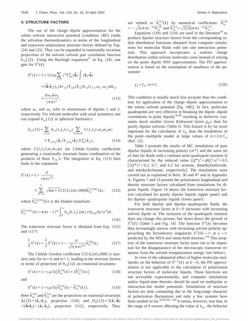
V. STRUCTURE FACTORS

The use of the charge–dipole approximation for thesolute–solvent interaction potential@condition ~48!# yieldsthe solvation thermodynamics in terms of the longitudinaland transverse polarization structure factors defined by Eqs.~24! and~25!. They can be expanded in rotationally invariantprojections of the solvent–solvent pair correlation functionhss(12). Using the Rayleigh expansion57 in Eq. ~24!, onegets forSL(k)

SL~k!51112pr(n,m

i nYnm* ~ k!E ~ e1"k!

3~ k"e2! j n~kr12!Ynm~ r12!hss~r 12,v1 ,v2!dr12

3dv1dv2

~4p!2, ~113!

wherev1 and v2 refer to orientations of dipoles 1 and 2,respectively. For solvent molecules with axial symmetry onecan expandhss(12) in spherical harmonics:

hss~12!5 (l 1l 2l

hss~ l 1l 2l ;r 12! (m1m2m

C~ l 1l 2l ;m1m2m!

3Yl 1m1~ e1!Yl 2m2

~ e2!Ylm* ~ r12!, ~114!

where C( l 1l 2l ;m1m2m) are Clebsh–Gordon coefficientsgenerating a rotationally invariant linear combination of theproducts of threeYlm’s. The integration in Eq.~113! thenleads to the expansion

SL~k!511r

~4p!3/2

3 (m50

`

A4m11C„11~2m!;000…hss11~2m!~k!, ~115!

wherehss11(2m)(k) is the Hankel transform:

hss11~2m!~k!54p~21!mE

0

`

hss„l 1l 2~2m!;r …j 2m~kr !r 2dr.

~116!

The transverse structure factor is obtained from Eqs.~115!and ~117!:

1

3SL~k!1

2

3ST~k!512

r

A3~4p!3/2hss

110~k!. ~117!

The Clebsh–Gordon coefficientC„11(2m),000… is non-zero only form50 andm51, leading to the structure factorsin terms of projection ofhss(12) on rotational invariants:

SL~k!511~r/3!@ hss110~k!12hss

112~k!# ~118!

and

ST~k!511~r/3!@ hss110~k!2hss

112~k!#. ~119!

Herehss110 andhss

112 are the projections on rotational invariantsD(12)5(e1"e2), projection ~110!, and Dk(12)53(e1"k)3( k"e2)2(e1"e2), projection ~112!, respectively. They

are related to hss11n(k) by numerical coefficients:hss

110

52A3(4p)23/2hss110 and hss

1125A15/2(4p)23/2hss112.

Equations~118! and ~119! are used in the literature59 toproduce dipolar structure factors from the corresponding ra-dial distribution functions obtained from computer simula-tions for molecular fluids with site–site interaction poten-tials. This approach incorporates a realistic chargedistribution within solvent molecular cores instead of relyingon the point–dipole~PD! approximation. The PD approxi-mation is based on the assumption of smallness of the pa-rameter

z25 l ss/s!1. ~120!

This condition is usually much less accurate than the condi-tion for application of the charge–dipole approximation tothe solute–solvent potential@Eq. ~48!#. In fact, molecularquadrupoles are very effective in breaking the dipole–dipolecorrelations in polar liquids,45,46 resulting in dielectric con-stants much smaller~lower Kirkwood factorgK) than forpurely dipolar solvents~Table I!. This feature is by far moreimportant for the calculation oflp than the breakdown ofthe point–multipole model at large values ofk>2p/ l ss

~Ref. 22!.Table I presents the results of MC simulations of pure

dipolar liquids of increasing polarity (m* ) and the same setof data for fluids with a constant axial quadrupole momentQcharacterized by the reduced value (Q* )25bQ2/s550.5@(Q* )250.2, 0.7, and 0.2 for acetone, dimethylsulfoxide,and tetrahydrofurane, respectively#. The simulations werecarried out as explained in Refs. 36 and 47 and in AppendixA. Figures 7 and 13 present the polarization longitudinal anddensity structure factors calculated from simulations for di-polar liquids. Figure 14 shows the transverse structure fac-tors calculated for purely dipolar liquids~upper panel! andfor dipolar–quadrupolar liquids~lower panel!.

For both dipolar and dipolar–quadrupolar fluids, thetransverse structure factor atk50 increases with increasingsolvent dipolem. The inclusion of the quadrupole momentdoes not change this picture, but slows down the growth ofST(0) ~Table I and Fig. 14!. The functionST(k) becomesthus increasingly narrow with increasing solvent polarity ap-proaching the ferroelectric singularityST(0)→` at y→`predicted by the MSA and mean-field theories.110 This prop-erty of the transverse structure factor turns out to be impor-tant for the disappearance of the microscopic transverse re-sponse from the solvent reorganization energy~see below!.

In view of the substantial effect of higher molecular mul-tipoles on the behavior ofSL,T(k) at k→0, the PD approxi-mation is not applicable to the calculation of polarizationstructure factors of molecular liquids. These functions arenot accessible experimentally, and computer simulationsand/or liquid-state theories should be used on multipolar orinteraction-site model potentials. Simulations of structurefactors are time consuming due to the long-range characterof polarization fluctuations and only a few systems havebeen studied so far.58,59,101–104It seems, however, true that, inthe range ofk vectors affecting the value oflp , the behavior



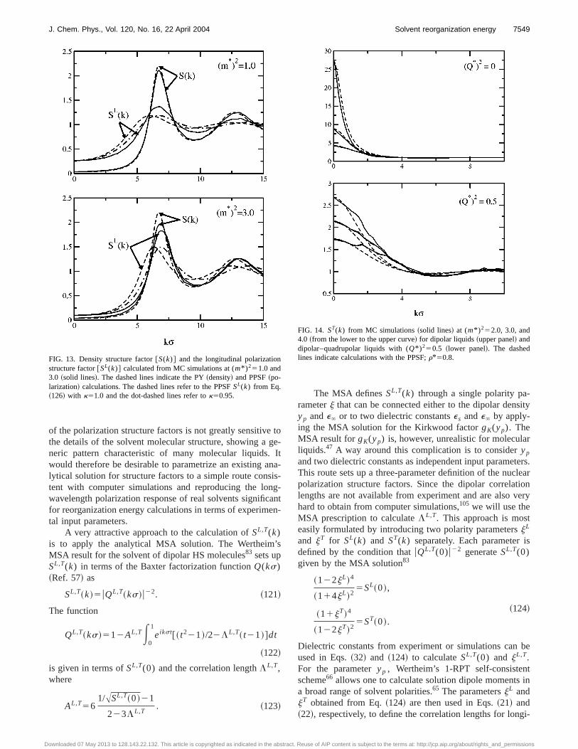
of the polarization structure factors is not greatly sensitive tothe details of the solvent molecular structure, showing a ge-neric pattern characteristic of many molecular liquids. Itwould therefore be desirable to parametrize an existing ana-lytical solution for structure factors to a simple route consis-tent with computer simulations and reproducing the long-wavelength polarization response of real solvents significantfor reorganization energy calculations in terms of experimen-tal input parameters.

A very attractive approach to the calculation ofSL,T(k)is to apply the analytical MSA solution. The Wertheim’sMSA result for the solvent of dipolar HS molecules83 sets upSL,T(k) in terms of the Baxter factorization functionQ(ks)~Ref. 57! as

SL,T~k!5uQL,T~ks!u22. ~121!

The function

QL,T~ks!512AL,TE0

1

eikst@~ t221!/22LL,T~ t21!#dt

~122!

is given in terms ofSL,T(0) and the correlation lengthLL,T,where

AL,T561/ASL,T~0!21

223LL,T. ~123!

The MSA definesSL,T(k) through a single polarity pa-rameterj that can be connected either to the dipolar densityyp ande` or to two dielectric constantses ande` by apply-ing the MSA solution for the Kirkwood factorgK(yp). TheMSA result forgK(yp) is, however, unrealistic for molecularliquids.47 A way around this complication is to consideryp

and two dielectric constants as independent input parameters.This route sets up a three-parameter definition of the nuclearpolarization structure factors. Since the dipolar correlationlengths are not available from experiment and are also veryhard to obtain from computer simulations,105 we will use theMSA prescription to calculateLL,T. This approach is mosteasily formulated by introducing two polarity parametersjL

and jT for SL(k) and ST(k) separately. Each parameter isdefined by the condition thatuQL,T(0)u22 generateSL,T(0)given by the MSA solution83

~122jL!4

~114jL!25SL~0!,

~124!~11jT!4

~122jT!25ST~0!.

Dielectric constants from experiment or simulations can beused in Eqs.~32! and ~124! to calculateSL,T(0) andjL,T.For the parameteryp , Wertheim’s 1-RPT self-consistentscheme66 allows one to calculate solution dipole moments ina broad range of solvent polarities.65 The parametersjL andjT obtained from Eq.~124! are then used in Eqs.~21! and~22!, respectively, to define the correlation lengths for longi-

FIG. 13. Density structure factor@S(k)# and the longitudinal polarizationstructure factor@SL(k)# calculated from MC simulations at (m* )251.0 and3.0 ~solid lines!. The dashed lines indicate the PY~density! and PPSF~po-larization! calculations. The dashed lines refer to the PPSFSL(k) from Eq.~126! with k51.0 and the dot-dashed lines refer tok50.95.

FIG. 14. ST(k) from MC simulations~solid lines! at (m* )252.0, 3.0, and4.0 ~from the lower to the upper curve! for dipolar liquids~upper panel! anddipolar–quadrupolar liquids with (Q* )250.5 ~lower panel!. The dashedlines indicate calculations with the PPSF;r*50.8.



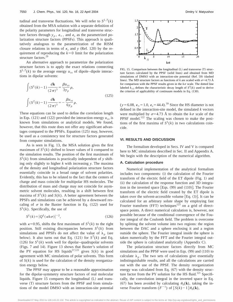
tudinal and transverse fluctuations. We will refer toSL,T(k)obtained from the MSA solution with a separate definition ofthe polarity parameters for longitudinal and transverse struc-ture factors throughyp , e` , andes as the parametrized po-larization structure factors~PPSFs!. This approach is quali-tatively analogous to the parametrization of the RISMclosure relations in terms ofes and y ~Ref. 120! by the re-quirement of reproducing thek50 limit for the polarizationstructure factors.29

An alternative approach to parametrize the polarizationstructure factors is to apply the exact relations connectingSL,T(k) to the average energyuss of dipole–dipole interac-tions in dipolar solvents:

E~SL~k!21!dk

~2p!35

buss

3ypr,

~125!

E~ST~k!21!dk

~2p!352

buss

6ypr.

These equations can be used to define the correlation lengthin Eqs.~121! and~122! provided the interaction energyuss isknown from simulations or analytical models. We found,however, that this route does not offer any significant advan-tages compared to the PPSFs. Equation~125! may, however,be used as a consistency test for structure factors generatedfrom computer simulations.

As is seen in Fig. 13, the MSA solution gives the firstmaximum ofSL(k) shifted to lower values ofk compared tothe simulation results. The position of the first maximum ofSL(k) from simulations is practically independent ofy shift-ing only slightly to higherk with increasingy. The maximaof the density and longitudinal polarization structure factorsessentially coincide in a broad range of solvent polarities.Evidently, this has to be related to the fact that the centers ofcharge and mass coincide for multipolar HS molecules. Thedistribution of mass and charge may not coincide for asym-metric solvent molecules, resulting in a shift between firstmaxima ofSL(k) andS(k). A better agreement between thePPSFs and simulations can be achieved by a downward res-caling of s in the Baxter function in Eq.~122! used forSL(k). Specifically, the use of

SL~k!5uQL~kks!u22, ~126!

with k50.95, shifts the first maximum ofSL(k) to the rightposition. Still existing discrepancies betweenSL(k) fromsimulations and PPSFs do not affect the value oflp ~seebelow!. It also turns out that Eq.~121! for ST(k) and Eq.~126! for SL(k) work well for dipolar–quadrupolar solvents~Figs. 7 and 14!. Figure 13 shows that Baxter’s solution ofthe PY equation for HS liquids57,121 gives S(k) in goodagreement with MC simulations of polar solvents. This formof S(k) is used for the calculation of the density reorganiza-tion energy below.

The PPSF may appear to be a reasonable approximationfor the dipolar-symmetry structure factors of real molecularliquids. Figure 15 compares the longitudinal~L! and trans-verse~T! structure factors from the PPSF and from simula-tions of the model DMSO with an interaction-site potential

(y56.08,e`51.0,es544.4).59 Since the HS diameter is notdefined in the interaction-site model, the simulatedk vectorswere multiplied bys54.73 Å to obtain theks scale of thePPSF model.122 The scaling was chosen to make the posi-tions of the first maxima ofSL(k) in two calculations coin-cide.

VI. RESULTS AND DISCUSSION

The formalism developed in Secs. IV and V is comparedhere to MC simulations described in Sec. II and Appendix A.We begin with the description of the numerical algorithm.

A. Calculation procedure

Numerical implementation of the analytical formalismincludes two components:~i! the calculation of the Fouriertransform of the electric field of the ET dipole~Fig. 1! and~ii ! the calculation of the response function and 3D integra-tion in the inverted space@Eqs.~99! and~110!#. The Fouriertransform of the electric field created by the ET dipole istaken over the solvent-accessible volume@Eq. ~3!#. It can becalculated for an arbitrary solute shape by employing fastFourier transform~FFT! techniques123 on a grid of direct-space points. A direct numerical calculation is, however, notpossible because of the conditional convergence of the Fou-rier integral of the Coulomb field. The problem is overcomeby splitting the solvent volume into two regions: the regionbetween the DAC and a sphere enclosing it and a regionoutside the sphere. The Fourier integral inside the sphere istaken numerically by the FFT and the Fourier integral out-side the sphere is calculated analytically~Appendix C!.

The polarization structure factors directly from MCsimulations and the PPSF were used in Eqs.~99! and~110! tocalculatelp . The two sets of calculations give essentiallyindistinguishable results, and all the calculations are carriedout with the use of the PPSF. The density reorganizationenergy was calculated from Eq.~67! with the density struc-ture factor from the PY solution for the HS fluid.121 Specifi-cally, the convolution integral in the inverted space in Eq.~67! has been avoided by calculatingu0(k), taking the in-verse Fourier transform (F21) of @S(k)21#u0(k),

FIG. 15. Comparison between the longitudinal~L! and transverse~T! struc-ture factors calculated by the PPSF~solid lines! and obtained from MDsimulations of DMSO with an interaction-site potential~Ref. 59! ~dashedlines!. The MD structure factors as functions ofk are scaled withs54.73 Åfor comparison with the PPSF results given in theks scale. The dotted linelabeledk1/2 defines the characteristic decay length ofST(k) used to derivethe criterion of applicability of continuum models in Eq.~130!.



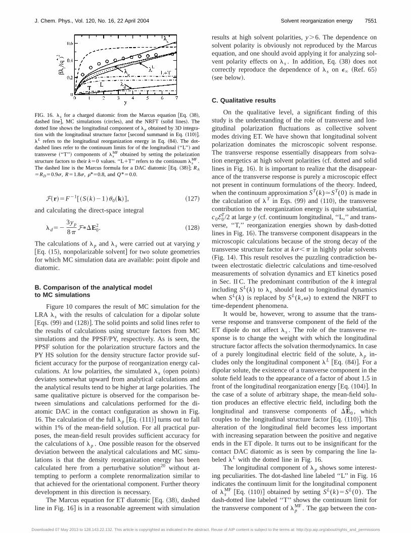
F~r !5F21@~S~k!21!u0~k!#, ~127!

and calculating the direct-space integral

ld523yp

8pF* DE0

2. ~128!

The calculations oflp andls were carried out at varyingy@Eq. ~15!, nonpolarizable solvent# for two solute geometriesfor which MC simulation data are available: point dipole anddiatomic.

B. Comparison of the analytical modelto MC simulations

Figure 10 compares the result of MC simulation for theLRA ls with the results of calculation for a dipolar solute@Eqs.~99! and~128!#. The solid points and solid lines refer tothe results of calculations using structure factors from MCsimulations and the PPSF/PY, respectively. As is seen, thePPSF solution for the polarization structure factors and thePY HS solution for the density structure factor provide suf-ficient accuracy for the purpose of reorganization energy cal-culations. At low polarities, the simulatedls ~open points!deviates somewhat upward from analytical calculations andthe analytical results tend to be higher at large polarities. Thesame qualitative picture is observed for the comparison be-tween simulations and calculations performed for the di-atomic DAC in the contact configuration as shown in Fig.16. The calculation of the fulllp @Eq. ~111!# turns out to fallwithin 1% of the mean-field solution. For all practical pur-poses, the mean-field result provides sufficient accuracy forthe calculations oflp . One possible reason for the observeddeviation between the analytical calculations and MC simu-lations is that the density reorganization energy has beencalculated here from a perturbative solution20 without at-tempting to perform a complete renormalization similar tothat achieved for the orientational component. Further theorydevelopment in this direction is necessary.

The Marcus equation for ET diatomic@Eq. ~38!, dashedline in Fig. 16# is in a reasonable agreement with simulation

results at high solvent polarities,y.6. The dependence onsolvent polarity is obviously not reproduced by the Marcusequation, and one should avoid applying it for analyzing sol-vent polarity effects onls . In addition, Eq.~38! does notcorrectly reproduce the dependence ofls on e` ~Ref. 65!~see below!.

C. Qualitative results

On the qualitative level, a significant finding of thisstudy is the understanding of the role of transverse and lon-gitudinal polarization fluctuations as collective solventmodes driving ET. We have shown that longitudinal solventpolarization dominates the microscopic solvent response.The transverse response essentially disappears from solva-tion energetics at high solvent polarities~cf. dotted and solidlines in Fig. 16!. It is important to realize that the disappear-ance of the transverse response is purely a microscopic effectnot present in continuum formulations of the theory. Indeed,when the continuum approximationST(k).ST(0) is made inthe calculation oflT in Eqs. ~99! and ~110!, the transversecontribution to the reorganization energy is quite substantial,c0E0

T/2 at largey ~cf. continuum longitudinal, ‘‘L,’’ and trans-verse, ‘‘T,’’ reorganization energies shown by dash-dottedlines in Fig. 16!. The transverse component disappears in themicroscopic calculations because of the strong decay of thetransverse structure factor atks,p in highly polar solvents~Fig. 14!. This result resolves the puzzling contradiction be-tween electrostatic dielectric calculations and time-resolvedmeasurements of solvation dynamics and ET kinetics posedin Sec. II C. The predominant contribution of thek integralincluding SL(k) to ls should lead to longitudinal dynamicswhenSL(k) is replaced bySL(k,v) to extend the NRFT totime-dependent phenomena.

It would be, however, wrong to assume that the trans-verse response and transverse component of the field of theET dipole do not affectls . The role of the transverse re-sponse is to change the weight with which the longitudinalstructure factor affects the solvation thermodynamics. In caseof a purely longitudinal electric field of the solute,lp in-cludes only the longitudinal componentlL @Eq. ~84!#. For adipolar solute, the existence of a transverse component in thesolute field leads to the appearance of a factor of about 1.5 infront of the longitudinal reorganization energy@Eq. ~104!#. Inthe case of a solute of arbitrary shape, the mean-field solu-tion produces an effective electric field, including both thelongitudinal and transverse components ofDE0 , whichcouples to the longitudinal structure factor@Eq. ~110!#. Thisalteration of the longitudinal field becomes less importantwith increasing separation between the positive and negativeends in the ET dipole. It turns out to be insignificant for thecontact DAC diatomic as is seen by comparing the line la-beledlL with the dotted line in Fig. 16.

The longitudinal component oflp shows some interest-ing peculiarities. The dot-dashed line labeled ‘‘L’’ in Fig. 16indicates the continuum limit for the longitudinal componentof ls

MF @Eq. ~110!# obtained by settingSL(k)5SL(0). Thedash-dotted line labeled ‘‘T’’ shows the continuum limit forthe transverse component oflp

MF . The gap between the con-

FIG. 16. ls for a charged diatomic from the Marcus equation@Eq. ~38!,dashed line#, MC simulations~circles!, and the NRFT~solid lines!. Thedotted line shows the longitudinal component oflp obtained by 3D integra-tion with the longitudinal structure factor@second summand in Eq.~110!#.lL refers to the longitudinal reorganization energy in Eq.~84!. The dot-dashed lines refer to the continuum limits for of the longitudinal~‘‘L’’ ! andtransverse~‘‘T’’ ! components ofls

MF obtained by setting the polarizationstructure factors to theirk50 values. ‘‘L1T’’ refers to the continuumls

MF .The dashed line is the Marcus formula for a DAC diatomic@Eq. ~38!#; RA

5RD50.9s, R51.8s, r*50.8, andQ* 50.0.



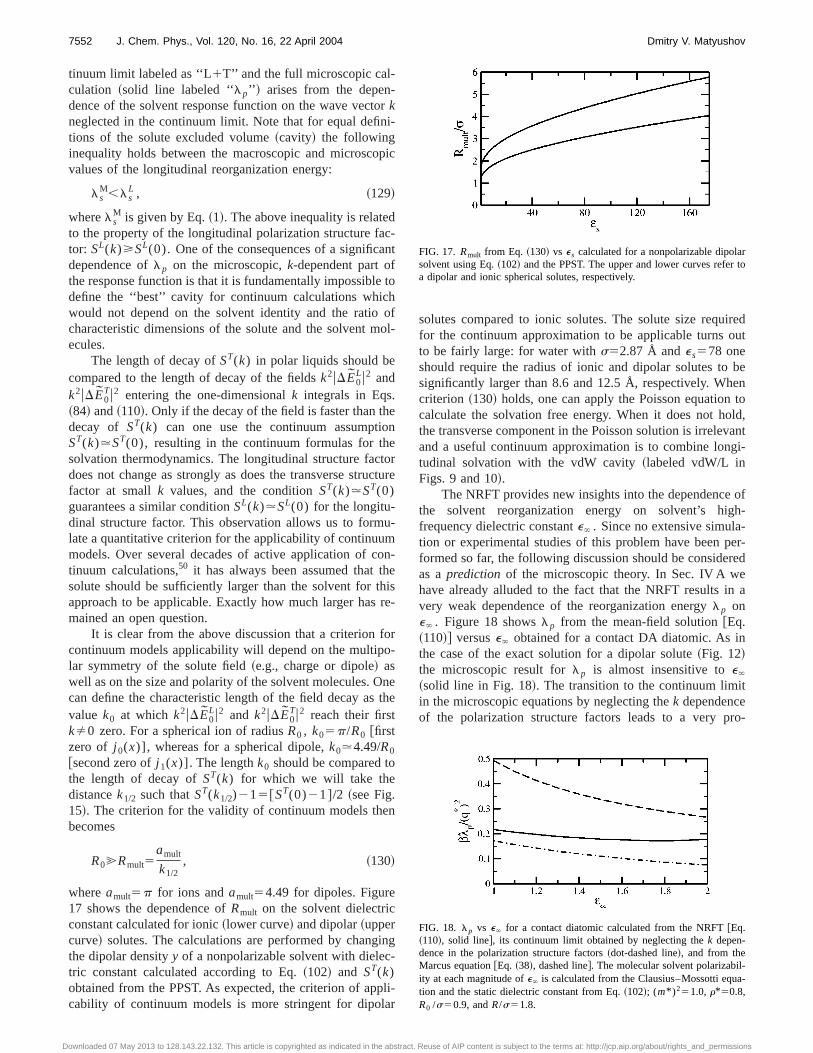
tinuum limit labeled as ‘‘L1T’’ and the full microscopic cal-culation ~solid line labeled ‘‘lp’’ ! arises from the depen-dence of the solvent response function on the wave vectorkneglected in the continuum limit. Note that for equal defini-tions of the solute excluded volume~cavity! the followinginequality holds between the macroscopic and microscopicvalues of the longitudinal reorganization energy:

lsM,ls

L , ~129!

wherelsM is given by Eq.~1!. The above inequality is related

to the property of the longitudinal polarization structure fac-tor: SL(k)>SL(0). One of theconsequences of a significantdependence oflp on the microscopic,k-dependent part ofthe response function is that it is fundamentally impossible todefine the ‘‘best’’ cavity for continuum calculations whichwould not depend on the solvent identity and the ratio ofcharacteristic dimensions of the solute and the solvent mol-ecules.

The length of decay ofST(k) in polar liquids should becompared to the length of decay of the fieldsk2uDE0

Lu2 andk2uDE0

Tu2 entering the one-dimensionalk integrals in Eqs.~84! and~110!. Only if the decay of the field is faster than thedecay of ST(k) can one use the continuum assumptionST(k).ST(0), resulting in the continuum formulas for thesolvation thermodynamics. The longitudinal structure factordoes not change as strongly as does the transverse structurefactor at smallk values, and the conditionST(k).ST(0)guarantees a similar conditionSL(k).SL(0) for the longitu-dinal structure factor. This observation allows us to formu-late a quantitative criterion for the applicability of continuummodels. Over several decades of active application of con-tinuum calculations,50 it has always been assumed that thesolute should be sufficiently larger than the solvent for thisapproach to be applicable. Exactly how much larger has re-mained an open question.

It is clear from the above discussion that a criterion forcontinuum models applicability will depend on the multipo-lar symmetry of the solute field~e.g., charge or dipole! aswell as on the size and polarity of the solvent molecules. Onecan define the characteristic length of the field decay as thevalue k0 at which k2uDE0

Lu2 and k2uDE0Tu2 reach their first

kÞ0 zero. For a spherical ion of radiusR0 , k05p/R0 @firstzero of j 0(x)], whereas for a spherical dipole,k0.4.49/R0

@second zero ofj 1(x)]. The lengthk0 should be compared tothe length of decay ofST(k) for which we will take thedistancek1/2 such thatST(k1/2)215@ST(0)21#/2 ~see Fig.15!. The criterion for the validity of continuum models thenbecomes

R0@Rmult5amult

k1/2, ~130!

whereamult5p for ions andamult54.49 for dipoles. Figure17 shows the dependence ofRmult on the solvent dielectricconstant calculated for ionic~lower curve! and dipolar~uppercurve! solutes. The calculations are performed by changingthe dipolar densityy of a nonpolarizable solvent with dielec-tric constant calculated according to Eq.~102! and ST(k)obtained from the PPST. As expected, the criterion of appli-cability of continuum models is more stringent for dipolar

solutes compared to ionic solutes. The solute size requiredfor the continuum approximation to be applicable turns outto be fairly large: for water withs52.87 Å andes578 oneshould require the radius of ionic and dipolar solutes to besignificantly larger than 8.6 and 12.5 Å, respectively. Whencriterion ~130! holds, one can apply the Poisson equation tocalculate the solvation free energy. When it does not hold,the transverse component in the Poisson solution is irrelevantand a useful continuum approximation is to combine longi-tudinal solvation with the vdW cavity~labeled vdW/L inFigs. 9 and 10!.

The NRFT provides new insights into the dependence ofthe solvent reorganization energy on solvent’s high-frequency dielectric constante` . Since no extensive simula-tion or experimental studies of this problem have been per-formed so far, the following discussion should be consideredas aprediction of the microscopic theory. In Sec. IV A wehave already alluded to the fact that the NRFT results in avery weak dependence of the reorganization energylp one` . Figure 18 showslp from the mean-field solution@Eq.~110!# versuse` obtained for a contact DA diatomic. As inthe case of the exact solution for a dipolar solute~Fig. 12!the microscopic result forlp is almost insensitive toe`

~solid line in Fig. 18!. The transition to the continuum limitin the microscopic equations by neglecting thek dependenceof the polarization structure factors leads to a very pro-

FIG. 17. Rmult from Eq. ~130! vs es calculated for a nonpolarizable dipolarsolvent using Eq.~102! and the PPST. The upper and lower curves refer toa dipolar and ionic spherical solutes, respectively.

FIG. 18. lp vs e` for a contact diatomic calculated from the NRFT@Eq.~110!, solid line#, its continuum limit obtained by neglecting thek depen-dence in the polarization structure factors~dot-dashed line!, and from theMarcus equation@Eq. ~38!, dashed line#. The molecular solvent polarizabil-ity at each magnitude ofe` is calculated from the Clausius–Mossotti equa-tion and the static dielectric constant from Eq.~102!; (m* )251.0, r*50.8,R0 /s50.9, andR/s51.8.



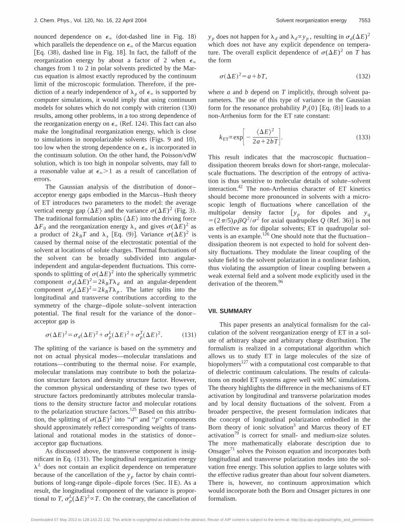
nounced dependence one` ~dot-dashed line in Fig. 18!which parallels the dependence one` of the Marcus equation@Eq. ~38!, dashed line in Fig. 18#. In fact, the falloff of thereorganization energy by about a factor of 2 whene`

changes from 1 to 2 in polar solvents predicted by the Mar-cus equation is almost exactly reproduced by the continuumlimit of the microscopic formulation. Therefore, if the pre-diction of a nearly independence oflp of e` is supported bycomputer simulations, it would imply that using continuummodels for solutes which do not comply with criterion~130!results, among other problems, in a too strong dependence ofthe reorganization energy one` ~Ref. 124!. This fact can alsomake the longitudinal reorganization energy, which is closeto simulations in nonpolarizable solvents~Figs. 9 and 10!,too low when the strong dependence one` is incorporated inthe continuum solution. On the other hand, the Poisson/vdWsolution, which is too high in nonpolar solvents, may fall toa reasonable value ate`.1 as a result of cancellation oferrors.

The Gaussian analysis of the distribution of donor–acceptor energy gaps embodied in the Marcus–Hush theoryof ET introduces two parameters to the model: the averagevertical energy gapDE& and the variances(DE)2 ~Fig. 3!.The traditional formulation splitsDE& into the driving forceDF0 and the reorganization energyls and givess(DE)2 asa product of 2kBT and ls @Eq. ~9!#. Variances(DE)2 iscaused by thermal noise of the electrostatic potential of thesolvent at locations of solute charges. Thermal fluctuations ofthe solvent can be broadly subdivided into angular-independent and angular-dependent fluctuations. This corre-sponds to splitting ofs(DE)2 into the spherically symmetriccomponentsd(DE)252kBTld and an angular-dependentcomponentsp(DE)252kBTlp . The latter splits into thelongitudinal and transverse contributions according to thesymmetry of the charge–dipole solute–solvent interactionpotential. The final result for the variance of the donor–acceptor gap is

s~DE!25sd~DE!21spL~DE!21sp

T~DE!2. ~131!

The splitting of the variance is based on the symmetry andnot on actual physical modes—molecular translations androtations—contributing to the thermal noise. For example,molecular translations may contribute to both the polariza-tion structure factors and density structure factor. However,the common physical understanding of these two types ofstructure factors predominantly attributes molecular transla-tions to the density structure factor and molecular rotationsto the polarization structure factors.125 Based on this attribu-tion, the splitting ofs(DE)2 into ‘‘ d’’ and ‘‘ p’’ componentsshould approximately reflect corresponding weights of trans-lational and rotational modes in the statistics of donor–acceptor gap fluctuations.

As discussed above, the transverse component is insig-nificant in Eq.~131!. The longitudinal reorganization energylL does not contain an explicit dependence on temperaturebecause of the cancellation of theyp factor by chain contri-butions of long-range dipole–dipole forces~Sec. II E!. As aresult, the longitudinal component of the variance is propor-tional toT, sp

L(DE)2}T. On the contrary, the cancellation of

yp does not happen forld andld}yp , resulting insd(DE)2

which does not have any explicit dependence on tempera-ture. The overall explicit dependence ofs(DE)2 on T hasthe form

s~DE!25a1bT, ~132!

wherea and b depend onT implicitly, through solvent pa-rameters. The use of this type of variance in the Gaussianform for the resonance probabilityPi(0) @Eq. ~8!# leads to anon-Arrhenius form for the ET rate constant:

kET}expF2^DE&2

2a12bTG . ~133!

This result indicates that the macroscopic fluctuation–dissipation theorem breaks down for short-range, molecular-scale fluctuations. The description of the entropy of activa-tion is thus sensitive to molecular details of solute–solventinteraction.42 The non-Arrhenius character of ET kineticsshould become more pronounced in solvents with a micro-scopic length of fluctuations where cancellation of themultipolar density factor @yp for dipoles and yq

5(2p/5)rbQ2/s2 for axial quadrupolesQ ~Ref. 36!# is notas effective as for dipolar solvents; ET in quadrupolar sol-vents is an example.126 One should note that the fluctuation–dissipation theorem is not expected to hold for solvent den-sity fluctuations. They modulate the linear coupling of thesolute field to the solvent polarization in a nonlinear fashion,thus violating the assumption of linear coupling between aweak external field and a solvent mode explicitly used in thederivation of the theorem.96

VII. SUMMARY

This paper presents an analytical formalism for the cal-culation of the solvent reorganization energy of ET in a sol-ute of arbitrary shape and arbitrary charge distribution. Theformalism is realized in a computational algorithm whichallows us to study ET in large molecules of the size ofbiopolymers127 with a computational cost comparable to thatof dielectric continuum calculations. The results of calcula-tions on model ET systems agree well with MC simulations.The theory highlights the difference in the mechanisms of ETactivation by longitudinal and transverse polarization modesand by local density fluctuations of the solvent. From abroader perspective, the present formulation indicates thatthe concept of longitudinal polarization embodied in theBorn theory of ionic solvation3 and Marcus theory of ETactivation79 is correct for small- and medium-size solutes.The more mathematically elaborate description due toOnsager71 solves the Poisson equation and incorporates bothlongitudinal and transverse polarization modes into the sol-vation free energy. This solution applies to large solutes withthe effective radius greater than about four solvent diameters.There is, however, no continuum approximation whichwould incorporate both the Born and Onsager pictures in oneformalism.



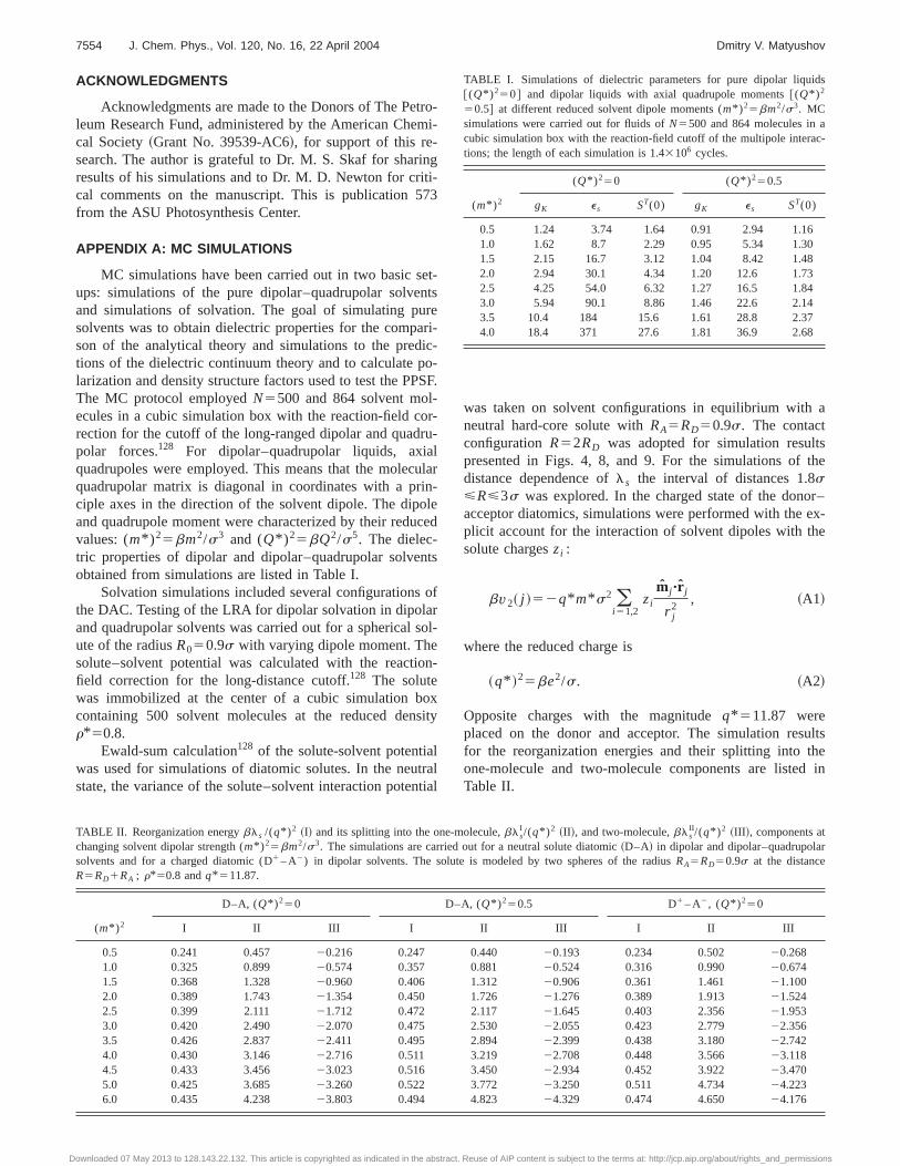
ACKNOWLEDGMENTS

Acknowledgments are made to the Donors of The Petro-leum Research Fund, administered by the American Chemi-cal Society~Grant No. 39539-AC6!, for support of this re-search. The author is grateful to Dr. M. S. Skaf for sharingresults of his simulations and to Dr. M. D. Newton for criti-cal comments on the manuscript. This is publication 573from the ASU Photosynthesis Center.

APPENDIX A: MC SIMULATIONS

MC simulations have been carried out in two basic set-ups: simulations of the pure dipolar–quadrupolar solventsand simulations of solvation. The goal of simulating puresolvents was to obtain dielectric properties for the compari-son of the analytical theory and simulations to the predic-tions of the dielectric continuum theory and to calculate po-larization and density structure factors used to test the PPSF.The MC protocol employedN5500 and 864 solvent mol-ecules in a cubic simulation box with the reaction-field cor-rection for the cutoff of the long-ranged dipolar and quadru-polar forces.128 For dipolar–quadrupolar liquids, axialquadrupoles were employed. This means that the molecularquadrupolar matrix is diagonal in coordinates with a prin-ciple axes in the direction of the solvent dipole. The dipoleand quadrupole moment were characterized by their reducedvalues: (m* )25bm2/s3 and (Q* )25bQ2/s5. The dielec-tric properties of dipolar and dipolar–quadrupolar solventsobtained from simulations are listed in Table I.

Solvation simulations included several configurations ofthe DAC. Testing of the LRA for dipolar solvation in dipolarand quadrupolar solvents was carried out for a spherical sol-ute of the radiusR050.9s with varying dipole moment. Thesolute–solvent potential was calculated with the reaction-field correction for the long-distance cutoff.128 The solutewas immobilized at the center of a cubic simulation boxcontaining 500 solvent molecules at the reduced densityr*50.8.

Ewald-sum calculation128 of the solute-solvent potentialwas used for simulations of diatomic solutes. In the neutralstate, the variance of the solute–solvent interaction potential

was taken on solvent configurations in equilibrium with aneutral hard-core solute withRA5RD50.9s. The contactconfigurationR52RD was adopted for simulation resultspresented in Figs. 4, 8, and 9. For the simulations of thedistance dependence ofls the interval of distances 1.8s<R<3s was explored. In the charged state of the donor–acceptor diatomics, simulations were performed with the ex-plicit account for the interaction of solvent dipoles with thesolute chargeszi :

bv2~ j !52q* m* s2 (i 51,2

zi

mj "r j

r j2

, ~A1!

where the reduced charge is

~q* !25be2/s. ~A2!

Opposite charges with the magnitudeq* 511.87 wereplaced on the donor and acceptor. The simulation resultsfor the reorganization energies and their splitting into theone-molecule and two-molecule components are listed inTable II.

TABLE I. Simulations of dielectric parameters for pure dipolar liquids@(Q* )250# and dipolar liquids with axial quadrupole moments@(Q* )2

50.5# at different reduced solvent dipole moments (m* )25bm2/s3. MCsimulations were carried out for fluids ofN5500 and 864 molecules in acubic simulation box with the reaction-field cutoff of the multipole interac-tions; the length of each simulation is 1.43106 cycles.

(m* )2

(Q* )250 (Q* )250.5

gK es ST(0) gK es ST(0)

0.5 1.24 3.74 1.64 0.91 2.94 1.161.0 1.62 8.7 2.29 0.95 5.34 1.301.5 2.15 16.7 3.12 1.04 8.42 1.482.0 2.94 30.1 4.34 1.20 12.6 1.732.5 4.25 54.0 6.32 1.27 16.5 1.843.0 5.94 90.1 8.86 1.46 22.6 2.143.5 10.4 184 15.6 1.61 28.8 2.374.0 18.4 371 27.6 1.81 36.9 2.68

TABLE II. Reorganization energybls /(q* )2 ~I! and its splitting into the one-molecule,blsI /(q* )2 ~II !, and two-molecule,bls

II /(q* )2 ~III !, components atchanging solvent dipolar strength (m* )25bm2/s3. The simulations are carried out for a neutral solute diatomic~D–A! in dipolar and dipolar–quadrupolarsolvents and for a charged diatomic (D1 – A2) in dipolar solvents. The solute is modeled by two spheres of the radiusRA5RD50.9s at the distanceR5RD1RA ; r*50.8 andq* 511.87.

(m* )2

D–A, (Q* )250 D–A, (Q* )250.5 D1 – A2, (Q* )250

I II III I II III I II III

0.5 0.241 0.457 20.216 0.247 0.440 20.193 0.234 0.502 20.2681.0 0.325 0.899 20.574 0.357 0.881 20.524 0.316 0.990 20.6741.5 0.368 1.328 20.960 0.406 1.312 20.906 0.361 1.461 21.1002.0 0.389 1.743 21.354 0.450 1.726 21.276 0.389 1.913 21.5242.5 0.399 2.111 21.712 0.472 2.117 21.645 0.403 2.356 21.9533.0 0.420 2.490 22.070 0.475 2.530 22.055 0.423 2.779 22.3563.5 0.426 2.837 22.411 0.495 2.894 22.399 0.438 3.180 22.7424.0 0.430 3.146 22.716 0.511 3.219 22.708 0.448 3.566 23.1184.5 0.433 3.456 23.023 0.516 3.450 22.934 0.452 3.922 23.4705.0 0.425 3.685 23.260 0.522 3.772 23.250 0.511 4.734 24.2236.0 0.435 4.238 23.803 0.494 4.823 24.329 0.474 4.650 24.176



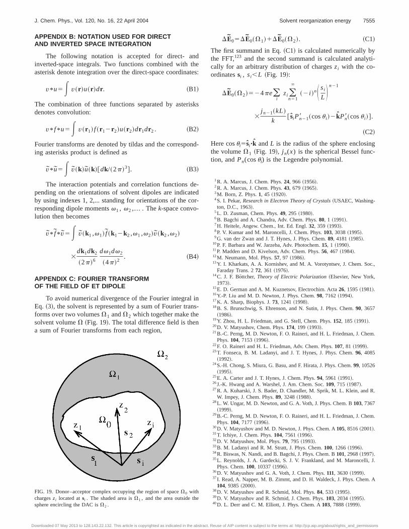
APPENDIX B: NOTATION USED FOR DIRECTAND INVERTED SPACE INTEGRATION

The following notation is accepted for direct- andinverted-space integrals. Two functions combined with theasterisk denote integration over the direct-space coordinates:

v* u5E v~r !u~r !dr . ~B1!

The combination of three functions separated by asterisksdenotes convolution:

v* f * u5E v~r1! f ~r12r2!u~r2!dr1dr2 . ~B2!

Fourier transforms are denoted by tildas and the correspond-ing asterisks product is defined as

v* u5E v~k!u~k!@dk/~2p!3#. ~B3!

The interaction potentials and correlation functions de-pending on the orientations of solvent dipoles are indicatedby using indexes 1, 2,... standing for orientations of the cor-responding dipole momentsv1 , v2 ,... . Thek-space convo-lution then becomes

v* f * v5E v~k1 ,v1! f ~k12k2 ,v1 ,v2!v~k2 ,v2!

3dk1dk2

~2p!6

dv1dv2

~4p!2. ~B4!

APPENDIX C: FOURIER TRANSFORMOF THE FIELD OF ET DIPOLE

To avoid numerical divergence of the Fourier integral inEq. ~3!, the solvent is represented by a sum of Fourier trans-forms over two volumesV1 andV2 which together make thesolvent volumeV ~Fig. 19!. The total difference field is thena sum of Fourier transforms from each region,

DE05DE0~V1!1DE0~V2!. ~C1!

The first summand in Eq.~C1! is calculated numerically bythe FFT,123 and the second summand is calculated analyti-cally for an arbitrary distribution of chargeszi with the co-ordinatessi , si,L ~Fig. 19!:

DE0~V2!524pe(i

zi (n51

`

~2 i !nS si

L D n21

3j n21~kL!

k@ si Pn218 ~cosu i !2 kPn8~cosu i !#.

~C2!

Here cosui5si "k andL is the radius of the sphere enclosingthe volumeV1 ~Fig. 19!, j n(x) is the spherical Bessel func-tion, andPn(cosui) is the Legendre polynomial.

1R. A. Marcus, J. Chem. Phys.24, 966 ~1956!.2R. A. Marcus, J. Chem. Phys.43, 679 ~1965!.3M. Born, Z. Phys.1, 45 ~1920!.4S. I. Pekar,Research in Electron Theory of Crystals~USAEC, Washing-ton, D.C., 1963!.

5L. D. Zusman, Chem. Phys.49, 295 ~1980!.6B. Bagchi and A. Chandra, Adv. Chem. Phys.80, 1 ~1991!.7H. Heitele, Angew. Chem., Int. Ed. Engl.32, 359 ~1993!.8P. V. Kumar and M. Maroncelli, J. Chem. Phys.103, 3038~1995!.9G. van der Zwan and J. T. Hynes, J. Phys. Chem.89, 4181~1985!.

10P. F. Barbara and W. Jarzeba, Adv. Photochem.15, 1 ~1990!.11P. Madden and D. Kivelson, Adv. Chem. Phys.56, 467 ~1984!.12M. Neumann, Mol. Phys.57, 97 ~1986!.13Y. I. Kharkats, A. A. Kornishev, and M. A. Vorotyntsev, J. Chem. Soc.,

Faraday Trans. 272, 361 ~1976!.14C. J. F. Bottcher, Theory of Electric Polarization~Elsevier, New York,

1973!.15E. D. German and A. M. Kuznetsov, Electrochim. Acta26, 1595~1981!.16Y.-P. Liu and M. D. Newton, J. Phys. Chem.98, 7162~1994!.17K. A. Sharp, Biophys. J.73, 1241~1998!.18B. S. Brunschwig, S. Ehrenson, and N. Sutin, J. Phys. Chem.90, 3657

~1986!.19Y. Zhou, H. L. Friedman, and G. Stell, Chem. Phys.152, 185 ~1991!.20D. V. Matyushov, Chem. Phys.174, 199 ~1993!.21B.-C. Perng, M. D. Newton, F. O. Raineri, and H. L. Friedman, J. Chem.

Phys.104, 7153~1996!.22F. O. Raineri and H. L. Friedman, Adv. Chem. Phys.107, 81 ~1999!.23T. Fonseca, B. M. Ladanyi, and J. T. Hynes, J. Phys. Chem.96, 4085

~1992!.24S.-H. Chong, S. Miura, G. Basu, and F. Hirata, J. Phys. Chem.99, 10526

~1995!.25E. A. Carter and J. T. Hynes, J. Chem. Phys.94, 5961~1991!.26J.-K. Hwang and A. Warshel, J. Am. Chem. Soc.109, 715 ~1987!.27R. A. Kuharski, J. S. Bader, D. Chandler, M. Sprik, M. L. Klein, and R.

W. Impey, J. Chem. Phys.89, 3248~1988!.28L. W. Ungar, M. D. Newton, and G. A. Voth, J. Phys. Chem. B103, 7367

~1999!.29B.-C. Perng, M. D. Newton, F. O. Raineri, and H. L. Friedman, J. Chem.

Phys.104, 7177~1996!.30D. V. Matyushov and M. D. Newton, J. Phys. Chem. A105, 8516~2001!.31T. Ichiye, J. Chem. Phys.104, 7561~1996!.32D. V. Matyushov, Mol. Phys.79, 795 ~1993!.33B. M. Ladanyi and R. M. Stratt, J. Phys. Chem.100, 1266~1996!.34R. Biswas, N. Nandi, and B. Bagchi, J. Phys. Chem. B101, 2968~1997!.35L. Reynolds, J. A. Gardecki, S. J. V. Frankland, and M. Maroncelli, J.

Phys. Chem.100, 10337~1996!.36D. V. Matyushov and G. A. Voth, J. Chem. Phys.111, 3630~1999!.37I. Read, A. Napper, M. B. Zimmt, and D. H. Waldeck, J. Phys. Chem. A

104, 9385~2000!.38D. V. Matyushov and R. Schmid, Mol. Phys.84, 533 ~1995!.39D. V. Matyushov and R. Schmid, J. Chem. Phys.103, 2034~1995!.40D. L. Derr and C. M. Elliott, J. Phys. Chem. A103, 7888~1999!.

FIG. 19. Donor–acceptor complex occupying the region of spaceV0 withchargeszi located atsi . The shaded area isV1 , and the area outside thesphere encircling the DAC isV2 .



41S. F. Nelsen, R. F. Ismagilov, K. E. Gentile, and D. R. Powell, J. Am.Chem. Soc.121, 7108~1999!.

42P. Vath, M. B. Zimmt, D. V. Matyushov, and G. A. Voth, J. Phys. Chem.B 103, 9130~1999!.

43P. Vath and M. B. Zimmt, J. Phys. Chem. A104, 2626~2000!.44X. Zhao, J. A. Burt, F. J. Knorr, and J. L. McHale, J. Phys. Chem. A105,

11110~2001!.45G. Stell, G. N. Patey, and J. S. Høye, Adv. Chem. Phys.18, 183 ~1981!.46A. Milischuk and D. V. Matyushov, J. Chem. Phys.118, 1859~2003!.47D. V. Matyushov and B. M. Ladanyi, J. Chem. Phys.110, 994 ~1999!.48A. M. Napper, I. Read, R. Kaplan, M. B. Zimmt, and D. H. Waldeck, J.

Phys. Chem. A106, 5288~2002!.49F. Raineri and H. Friedman, J. Chem. Phys.98, 8910~1993!.50C. J. Cramer and D. G. Truhlar, Chem. Rev.~Washington, D.C.! 99, 2161

~1999!.51R. M. Lynden-Bell, AIP Conf. Proc.492, 3 ~1999!.52B. M. Ladanyi and M. S. Skaf, Annu. Rev. Phys. Chem.44, 335 ~1993!.53L. R. Pratt and D. Chandler, J. Chem. Phys.67, 3683~1977!.54D. Chandler, Phys. Rev. E48, 2898~1993!.55X. Song, D. Chandler, and R. A. Marcus, J. Phys. Chem.100, 11954

~1996!.56X. Song and D. Chandler, J. Chem. Phys.108, 2594~1998!.57C. G. Gray and K. E. Gubbins,Theory of Molecular Liquids~Clarendon,

Oxford, 1984!.58F. O. Raineri, H. Resat, and H. L. Friedman, J. Chem. Phys.96, 3068

~1992!.59M. S. Skaf, J. Chem. Phys.107, 7996~1997!.60D. Ben-Amotz and D. R. Herschbach, J. Phys. Chem.90, 1038~1990!.61D. Ben-Amotz and K. G. Willis, J. Phys. Chem.97, 7736~1993!.62R. Schmid and D. V. Matyushov, J. Phys. Chem.99, 2393~1995!.63D. V. Matyushov and R. Schmid, J. Chem. Phys.105, 4729~1996!.64S. W. Rick and S. J. Stuart,Reviews in Computational Chemistry~Wiley-

VCH, New York, 2002!, Vol. 18, p. 89.65S. Gupta and D. V. Matyushov, J. Phys. Chem. A108, ASAP ~2004!.66M. S. Wertheim, Mol. Phys.37, 83 ~1979!.67V. Venkatasubramanian, K. E. Gubbins, C. G. Gray, and C. C. Joslin,

Mol. Phys.52, 1411~1984!.68C. G. Joslin, C. G. Gray, and K. E. Gubbins, Mol. Phys.54, 1117~1985!.69D. Ben-Amotz and I. P. Omelyan, J. Chem. Phys.115, 9401~2001!.70M. B. Zimmt and D. H. Waldeck, J. Phys. Chem. A107, 3580~2003!.71L. Onsager, J. Am. Chem. Soc.58, 1486~1936!.72J. G. Kirkwood, J. Chem. Phys.2, 351 ~1934!.73R. H. Wood, J. R. Qulnt, and J.-P. E. Groller, J. Phys. Chem.85, 3944

~1981!.74M. Berg, J. Phys. Chem. A102, 17 ~1998!.75J. Jeon and H. J. Kim, J. Chem. Phys.119, 8606~2003!.76R. A. Marcus, J. Phys. Chem.93, 3078~1989!.77C. H. Wang,Spectroscopy of Condensed Media~Academic, Orlando, FL,

1985!.78B. M. Ladanyi and M. Maroncelli, J. Chem. Phys.109, 3204~1998!.79R. A. Marcus, Rev. Mod. Phys.65, 599 ~1993!.80D. V. Matyushov and G. A. Voth, J. Chem. Phys.113, 5413~1999!.81A. Milischuk and D. V. Matyushov, J. Phys. Chem. A106, 2146~2002!.82The solvent reorganization energy is defined as the equilibrium free en-

ergy of solvation of the ET dipole. The approach used here can be appliedto a DAC with an arbitrary charge as long as the solute charge does notchange the spectrum of fluctuations of the solvent~LRA!.

83M. S. Wertheim, J. Chem. Phys.55, 4291~1971!.84D. Y. C. Chan, D. J. Mitchell, and B. W. Ninham, J. Chem. Phys.70,

2946 ~1979!.85J. S. Høye and G. Stell, J. Chem. Phys.73, 461 ~1980!.86H. E. Stanley,Introduction to Phase Transitions and Critical Phenomena

~Oxford University Press, New York, 1987!.87The charges of the solute interact only with optical phonons changing the

local charge distribution in the solvent. Therefore thermal excitations,leading to a parallel tilt of the dipoles, can be neglected.

88J. P. Hansen and I. R. McDonald,Theory of Simple Liquids~Academic,Orlando, FL, 1986!.

89J. T. Hupp, Y. Dong, R. L. Blackbourn, and H. Lu, J. Phys. Chem.97,3278 ~1993!.

90W. Rocchia, E. Alexov, and B. Honig, J. Phys. Chem. B105, 6507~2001!.

91W. Rocchia, S. Sridharan, A. Nicholls, E. Alexov, A. Chiabrera, and B.Honig, J. Comput. Chem.23, 128 ~2002!.

92B. Berne, J. Chem. Phys.62, 1154~1975!.93A. Chandra, D. Wei, and G. N. Patey, J. Chem. Phys.99, 4926~1993!.94B. Bagchi and N. Gayathri, inAdvances in Chemical Physics, edited by J.

Jortner and M. Bixon~Wiley, New York, 1999!, Vol. 107, p. 1.95A. A. Ovchinnikov and M. Y. Ovchinnikova, Sov. Phys. JETP29, 688

~1969!.96R. Kubo,Lectures in Theoretical Physics~Interscience, New York, 1959!,

Vol. 1, p. 120.97H. C. Andersen and D. Chandler, J. Chem. Phys.57, 1918~1972!.98J. S. Høye and G. Stell, J. Chem. Phys.61, 562 ~1974!.99Short-range and long-range interactions can be distinguished based on the

convergence property of the second virial coefficient. The latter divergesfor radial interaction potentials}1/r d at d<3 ~long-range potential! andis finite atd.3 ~short-range potential!.

100N. Mataga,Molecular Interactions and Electronic Spectra~Dekker, NewYork, 1970!.

101M. S. Skaf and B. M. Ladanyi, J. Chem. Phys.102, 6542~1995!.102P. A. Bopp, A. A. Kornyshev, and G. Sutmann, Phys. Rev. Lett.76, 1280

~1996!.103B.-C. Perng and B. M. Ladanyi, J. Chem. Phys.110, 6389~1999!.104I. P. Omelyan, Mol. Phys.93, 123 ~1998!.105M. Lilichenko and D. V. Matyushov, J. Chem. Phys.119, 1559~2003!.106D. V. Matyushov and G. A. Voth, J. Phys. Chem. A103, 10981~1999!.107J. Richardi and P. H. Fries, J. Mol. Liq.88, 209 ~2000!.108D. V. Matyushov and B. M. Ladanyi, J. Chem. Phys.108, 6362~1998!.109G. Fischer,Vibronic Coupling~Academic, London, 1984!.110J. S. Høye and G. Stell, J. Chem. Phys.64, 1952~1976!.111L. R. Pratt, Mol. Phys.40, 347 ~1980!.112M. J. Thompson, K. S. Schweizer, and D. Chandler, J. Chem. Phys.76,

1128 ~1982!.113J. Cao and B. J. Berne, J. Chem. Phys.99, 2902~1993!.114E. L. Pollock, B. J. Alder, and G. N. Patey, Physica A108, 14 ~1981!.115H. Li and M. Kardar, Phys. Rev. A46, 6490~1992!.116D. V. Matyushov, J. Chem. Phys.120, 1375~2004!.117A singularity of the integrand in Eq.~95! in fact appears atk* defined by

the conditionSL12A50. This pole is responsible for longitudinal polar-ization waves generated in a polar solvent by the insertion of the solute.However, this singularity gives a negligible contribution to the integraland is not considered here.

118A. Tani, D. Henderson, and J. A. Barker, Mol. Phys.48, 863 ~1983!.119J. S. Bader and B. J. Berne, J. Chem. Phys.104, 1293~1996!.120P. J. Rossky and B. M. Pettitt, Mol. Phys.50, 1263~1983!.121R. J. Baxter, J. Chem. Phys.52, 4559~1970!.122The effective HS diameter of DMSO calculated by fitting the solvent

compressibility to that given by the generalized van der Waals equation is4.95 Å. The compressibility of the ISM fluid used to represent DMSOmay be, however, different from the compressibility of the real solvent.

123W. H. Press, S. A. Teukolsky, W. T. Vetterling, and B. P. Flannery,Nu-merical Recipes in Fortran 77: The art of scientific computing~Cam-bridge University Press, Cambridge, England, 1996!.

124A strong dependence one` will appear in any theory of ET reorganiza-tion that implements an additive correction for electronic polarizabilityeffects not entangled with the nonlocal response functions. For instance,the RISM formulation in Ref. 29 relies on an additive correction thedependence one` in which is as strong as in the Marcus formula.

125H. L. Friedman,A Course in Statistical Mechanics~Prentice-Hall, Engle-wood Cliffs, NJ, 1985!.

126I. Read, R. Kaplan, M. B. Zimmt, and D. H. Waldeck, J. Am. Chem. Soc.121, 10976~1999!.

127D. N. LeBard, M. Lilichenko, D. V. Matyushov, Y. A. Berlin, and M. A.Ratner, J. Phys. Chem. B107, 14509~2003!.

128M. P. Allen and D. J. Tildesley,Computer Simulation of Liquids~Claren-don, Oxford, 1996!.



Documents

Solvent reorganization energy of electron-transfer reactions in polar solvents