Embed Size (px)
Citation preview

The Pennsylvania State University
The Graduate School
Eberly College of Science
SOLVATION AND ELECTRON TRANSFER
IN IONIC LIQUIDS
A Dissertation in
Chemistry
by
Min Liang
© 2012 Min Liang
Submitted in Partial Fulfillment of the Requirements
for the Degree of
Doctor of Philosophy
August 2012

ii
The dissertation of Min Liang was reviewed and approved* by the following:
Mark Maroncelli Professor of Chemistry Dissertation Adviser Chair of Committee James B. Anderson Professor of Chemistry Evan Pugh Professor John B. Asbury Professor of Chemistry John H. Golbeck Professor of Biochemistry and Biophysics Professor of Chemistry Barbara J. Garrison Shapiro Professor of Chemistry Head of the Department of Chemistry * Signatures are on file in the Graduate School.

iii
ABSTRACT
The complete solvation response of coumarin 153 (C153) in 21 neat ionic liquids
(ILs) has been determined over the time range from 100 fs to 20 ns by combining broad-
band fluorescence upconversion (FLUPS) and time-correlated single photon counting
(TCSPC) measurements. The 80 fs time resolution of FLUPS provides accurate results for
the fast dynamics and the long time window (20 ns) of TCSPC enables observation of the
slow portion of the dynamics. These complete solvation response functions are compared
to the solvation dynamics predicted by a simple dielectric continuum model. This
dielectric continuum model works well in conventional solvents. However, the dynamics
predicted in most ionic liquids are systematically faster than those observed, on average by
a factor of 3–5.
To bridge the knowledge gap between neat ILs and conventional solvents, the
solvation dynamics of C153 in the mixture of a simple ionic liquid [Im41][BF4] and the
prototypical dipolar solvent acetonitrile has been studied. This mixture was chosen because
it is expected to exhibit the simplest behavior without much preferential solvation is not
expected to complicate interpretation due to the similar ‘polarity’ of acetonitrile and
[Im41][BF4]. The solvation energies of C153 in this mixture were determined and the
complete solvation dynamics of C153 were measured and compared to simple dielectric
continuum predictions. In addition, the rotational dynamics of C153 in the mixtures of
[Im41][BF4] and acetonitrile were studied. The rotation times <rot> of C153 vary with
viscosity in the manner <rot>p with p= 0.9.
Steady-state and picosecond time-resolved emission spectroscopy are used to
monitor the bimolecular electron transfer reaction between the electron acceptor 9,10-

iv
dicyanoanthracene in its S1 state and the donor N,N-dimethylaniline in a variety of ionic
liquids and several conventional solvents. Detailed study of this quenching reaction was
undertaken in order to better understand why rates reported for similar diffusion-limited
reactions in ionic liquids sometimes appear much higher than expected given the viscous
nature of these liquids. Consistent with previous studies, Stern-Volmer analyses of steady-
state and lifetime data provide effective quenching rate constants kq, which are often 10
to100-fold larger than simple predictions for diffusion-limited rate constants kD in ionic
liquids. Similar departures from kD are also observed in conventional organic solvents
having comparably high viscosities, indicating that this behavior is not unique to ionic
liquids. A more complete analysis of the quenching data using a model combining
approximate solution of the spherically symmetric diffusion equation with a Marcus-type
description of electron transfer reveals the reasons for frequent observation of kq kD.
The primary cause is that the high viscosities typical of ionic liquids emphasize the
transient component of diffusion-limited reactions, which renders the interpretation of rate
constants derived from Stern-Volmer analyses ambiguous. Using a more appropriate
description of the quenching process enables satisfactory fits of data in both ionic liquid
and conventional solvents using a single set of physically reasonable electron transfer
parameters. Doing so requires diffusion coefficients in ionic liquids to exceed
hydrodynamic predictions by significant factors, typically in the range of 3-10. Direct
NMR measurements of solute diffusion confirm this enhanced diffusion in ionic liquids.

v
Table of Contents
LIST OF FIGURES ............................................................................................. viii
LIST OF TABLES ................................................................................................. xi
GLOSSARY OF ACRONYMS ............................................................................ xii
ACKNOWLEDGMENTS ................................................................................... xiv
Chapter 1. Introduction ........................................................................................... 1
1.1. Ionic Liquids ............................................................................................. 1
1.2. Solvation Dynamics .................................................................................. 3
1.3. Bimolecular Electron Transfer ................................................................. 5
Notes and References: ................................................................................................ 6
Chapter 2. Experimental and Data Analysis Methods ......................................... 9
2.1 Experimental Methods ................................................................................. 9
2.1.1. Materials ............................................................................................... 9
2.1.2. Steady-State Measurements ................................................................. 11
2.1.3. Time- Correlated Single Photon Counting Measurements ................. 12
2.1.4. Fluorescence Up-Conversion Measurements ...................................... 14
2.1.5. Diffusion Measurements ...................................................................... 15
2.2. Data Analysis Methods ........................................................................... 16
2.2.1. Deconvolution of TCSPC Decays ........................................................ 16

vi
2.2.2. Reconstruction and Fitting of Time-Resolved Spectra ........................ 18
2.2.3. Solvation Dynamics Calculation and the Time-Zero Spectrum ........ 222
2.2.4. Anisotropy Analysis ............................................................................. 25
Notes and References ........................................................................................... 29
Chapter 3. Solvation Dynamics of Neat Ionic Liquids ....................................... 30
3.1. Introduction ............................................................................................. 30
3.2. Experimental Methods ............................................................................ 31
3.3. Results and Discussion ........................................................................... 35
3.3.1. Solvation Energies ............................................................................... 35
3.3.2. Spectral / Solvation Response Functions ............................................ 39
3.3.3. Comparisons to Dielectric Continuum Predictions ............................ 50
3.4. Summary and Conclusions ..................................................................... 59
Notes and Refrerences: ........................................................................................ 60
Chapter 4. Solvation and Rotational Dynamics in a Prototypical Ionic Liquid
+ Dipolar Solvent Mixture: Coumarin 153 in 1-Butyl-3-Methylimidazolium
Tetrafluoroborate + Acetonitrile .......................................................................... 65
4.1. Introduction ........................................................................................... 65
4.2. Experimental Methods .......................................................................... 66
4.3. Results and Discussion ......................................................................... 70
4.3.1. Physical Properties of the Mixtures ................................................... 70

vii
4.3.2. C153 Spectra and Energies ................................................................ 77
4.3.3. C153 Rotational Dynamics ............................................................... 82
4.3.4. Solvation Dynamics ............................................................................ 84
4.4. Summary and Conclusions ................................................................... 91
Notes and References ......................................................................................... 92
Chapter 5. Experimental Bimolecular Electron Transfer Between the 9,10-
dicyanoanthracene and N,N-dimethylaniline in Ionic Liquids .......................... 94
5.1. Introduction ............................................................................................. 95
5.2. Experimental Methods .......................................................................... 100
5.3. Modeling the Time-Dependent Quenching Process ............................. 102
5.3.1. The Formalism .................................................................................. 102
5.3.2. The Specification of Model Parameters ........................................... 107
5.4. Results and Discussion ......................................................................... 113
5.4.1. General Features of the Quenching Data ......................................... 113
5.4.2. Fitting to the Reaction Model ............................................................ 123
5.4.3. Interpretation of the DCA+DMA Reaction ....................................... 135
5.5. Summary and Conclusions ................................................................... 144
Notes and References ......................................................................................... 147

viii
LIST OF FIGURES
Figure 1.1: Structures of typical ionic liquids components. ..................................... 2
Figure 1.2: 6 Diagram of solvation dynamics for a typical polar solvent. ............... 3
Figure 2.1: Structures of the ionic liquid components studied and their
abbreviations. ......................................................................................................................... 9
Figure 2.2: Structures of probe coumarin 153 (C153), the electron acceptor (DCA)
and donor (DMA). ................................................................................................................ 10
Figure 2.3: Time-correlated single photon counting setup ..................................... 13
Figure 2.4:5 Schematic of the broadband Fluorescence UP-conversion
Spectrometer (FLUPS). ........................................................................................................ 14
Figure 2.5: Representative experimental data ........................................................ 18
Figure 2.6: The deconvoluted time-resolved spectra of C153 in [Im41][BF4]. ....... 20
Figure 2.7: Example time-dependent spectral parameters obtained from the spectra
in Fig 2.6. ............................................................................................................................. 21
Figure 2.8: Representative steady-state spectra. ..................................................... 23
Figure 2.9:8 A diagram of the fluorescence anisotropy measurement. ................... 26
Figure 3.1: Solvation contribution to the free energy change and reorganization
energy ................................................................................................................................... 37
Figure 3.2: Time-resolved emission spectra of C153 in [Pr51][Tf2N]. ................... 39
Figure 3.3: Illustration of the combination of FLUPS and TCSPC. ...................... 41
Figure 3.4: Time evolution of the peak frequencies pk(t) of C153 in the
imidazolium [Imn1][Tf2N] and pyrrolidinium [Prn1][Tf2N] series of ionic liquids. ............. 43

ix
Figure 3.5: Representative spectral response functions (points) and fits ............... 45
Figure 3.6: Correlation of the Gaussian frequency G with the inverse of the
reduced cation+anion reduced mass. ................................................................................... 48
Figure 3.7: Correlation of the integral time associated with the stretched
exponential component with solvent viscosity. ................................................................... 49
Figure 3.8: Dielectric relaxation and calculated solvation response functions of
[Im41][Tf2N]. ........................................................................................................................ 55
Figure 3.9: Comparison of measured C153 spectra response functions (black
curves) with dielectric continuum model predictions .......................................................... 57
Figure 3.10: Comparison of the times required for predicted and observed Sv(t) at
certain values ........................................................................................................................ 58
Figure 4.1: Measured and literature viscosity values of the mixtures. ................... 71
Figure 4.2: Plots of reaction field factor ................................................................ 73
Figure 4.3: Measured and simulated diffusion coefficients of the mixtures. .......... 74
Figure 4.4: Observed and Stokes-Einstein predicted diffusion coefficients. .......... 76
Figure 4.5: Steady state absorption and emission spectra of C153 ......................... 77
Figure 4.7: The solvation free energy and reorganization energy. ......................... 81
Figure 4.8: Plot of the rotation times vs. viscosities. .............................................. 84
Figure 4.9: Representative time-resolved spectra of C153 in the xIL= 0.5 mixture 85
Figure 4.10: Observed solvation response functions. ............................................. 87
Figure 4.11: Solvation times vs solvent viscosity ................................................... 88
Figure 4.12: Some representative measured and predicted S(t). ............................. 89

x
Figure 4.13: Comparison of the solvation response times of measured and
predicted response functions at certain S(t) values .............................................................. 90
Figure 5.1: Steady-state (top) and timeresolved (bottom) spectra of DCA in
[N3111][Tf2N] at 298 K. ...................................................................................................... 114
Figure 5.2: Representative steady-state emission spectra .................................... 116
Figure 5.3: Stern-Volmer plots of quenching efficiencies in [Pr41][Tf2N] .......... 117
Figure 5.4: Correlation between the ratio of quenching rate constants kq obtained
from Stern-Volmer plots at 0.1 M DMA to diffusion-controlled rate constant kD. ........... 121
Figure 5.5: VFT fitting ......................................................................................... 124
Figure 5.6: Fits of time-resolved DCA decays in [Pr41][Tf2N] ............................ 131
Figure 5.7: Fits of DCA quenching data .............................................................. 132
Figure 5.8: Some features of the electron transfer model applied ....................... 137
Figure 5.9: Model calculations illustrating the dependence of the quenching
reaction upon solution viscosity ......................................................................................... 141

xi
LIST OF TABLES
Table 3.1: Ionic Liquids Studied ............................................................................ 32
Table 3.2: Summary of C153 Fequencies and Energies ......................................... 36
Table 3.3: Parameterization of Spectral Response Data ......................................... 46
Table 3.4: Dielectric Dispersion Data Used ........................................................... 52
Table 4.1: Mixtures studied and some of their properties. ...................................... 72
Table 4.2: Summary of limiting frequencies and parameters of fits of S(t) data to
Eq. 4.10. ............................................................................................................................... 78
Table 4.3: Parameters of Biexponential Fits to Fluorescence Anisotropy Data .... 82
Table 5.1: Diffusion-Limited Bimolecular Reactions in ILs .................................. 96
Table 5.2: Summary of Model Parameters used in Fitting Quenching Data ........ 108
Table 5.3: Representative Quenching Data in [Pr41][Tf2N] at 298 K ................... 117
Table 5.4: Stern-Volmer Characterization of Steady-State and Time-Resolved
Quenching Data .................................................................................................................. 120
Table 5.5: Summary of Temperature-Dependent Fits to Viscosity Data ............. 125
Table 5.6: Summary of Fit Results ....................................................................... 128

xii
GLOSSARY OF ACRONYMS
A anion
ACN acetonitrile
C cation
C153 coumarin 153
CHX cyclohexane
D donor
DCA 9,10-dicyanoanthracene
DMA N,N-dimethylaniline
EG ethylene glycol
F fluorophore
FLUPS fluorescence up-conversion spectroscopy
FWHM full width at half maximum
G Gaussian function
GLY glycerol
IL ionic liquid
IRF instrumental response function
OD optical density
Q quencher
SE Stokes-Einstein
SS steady-state
SV Stern-Volmer
TCSPC time-correlated single photon counting

xiii
TR time-resolved
vdW van der Waals
VFT Vogel-Fulcher-Tammann

xiv
ACKNOWLEDGMENTS
My deepest gratitude goes to my advisor, Prof. Mark Maroncelli, for his scientific
guidance and continuous support throughout my graduate studies. His broad knowledge
in the field and enthusiasm for science has always been prompting me to learn. The
charm of his personality makes my life much easier and happier in his group. Because of
him, I enjoyed my five years of graduate school at Penn State. I feel so fortunate and
honored to work with him.
I would also like to thank my committee members Prof. James Anderson, Prof.
John Asbury and Prof. John Golbeck for giving me scientific advice. Their examples as
researchers will serve as guidelines for my academic career. I wish to extend my warmest
thanks to my collaborators Xinxing Zhang and Prof. Nikolaus Ernsting from Humboldt
University of Berlin. I thank Dr. Gary Baker who synthesized the pyrrolidinium ionic
liquids for my research. I would like to acknowledge the past and present Maroncelli
group members, Dr. Sergey Arzhantsev, Dr. Hui Jin, Jing Dong, Dr. Lillian Li, Jens
Breffke, Dr. Durba Roy, Anne Kaintz, Dr. Minako Kondo, with whom working in the lab
is a pleasure. In particular, I would like to thank Sergey who introduced me to our laser
systems and gave me tremendous help in the lab.
I am heartily thankful to my father, Weishuan Liang, who is always optimistic to
life and passes this positive character to me. I thank my mother, Meirong Liu for her
unconditional love and support. I would like to thank my six-month old son Lele (Eric)
who brings me a lot of happiness and the best title ever as a mom. Most of all, I thank my
husband Peng, for his love and encouragement over these many years. His broad

xv
knowledge makes him my personal Wikipedia. I am very proud and happy to have him
around. To them, I dedicate this dissertation.
1
Chapter 1. Introduction
1.1.Ionic Liquids
An ionic liquid (IL) is a salt having a freezing point below 100°C. Many ILs
remain liquid even at room temperature. Room temperature ionic liquids have been
known for about a century. The first observation of a room temperature ionic liquid was
reported by Paul Walden in 1914,1 but little research was performed on low melting salts
until 1992 when Wilkes and Zaworotko2 described the synthesis of 1-ethyl-3-
methylimidazolium based ionic liquids which were both air and water stable. Figure 1.1
shows some typical cations and anions of ionic liquids.
Ionic liquids have attracted tremendous attention due to their distinctive
properties, like the low volatility, intrinsic conductivity, high thermal stability and
tailorability. Currently, applications of ionic liquids permeate most fields of chemistry.
Among other applications, ionic liquids are being used as electrolytes in photovoltaic
cells3 and supercapacitors4, as green solvents for synthesis and catalysis, as separation
tools for mixtures, and as media for storage and transport of toxic gases5. For all of these
emerging applications, an understanding of the basic physical chemistry of ILs and how
they behave as solvent media for chemical reactions is essential.
Most chemical reactions take place in solution, which makes it very important to
choose the proper solvent. The tailorability of ionic liquids makes them stand out as
“designer solvents”. For example, the alkyl chains of the cation, or less commonly the
anion, can be easily varied to make a solvent of the desired size, viscosity and polarity.

2
For fundamental studies, it is thus easy to produce a series of ILs with variable properties.
In addition, ionic liquids can be easily prepared through simple ion exchange reactions.
Figure 1.1: Structures of typical ionic liquids components.
Ionic liquids are often used in conjunction with conventional organic solvents as a
means of increasing the fluidity and conductivity of these high-viscosity solvents. Thus,
there are practical reasons for understanding solvation in mixtures of ILs with
conventional solvents. Another reason for studying such mixtures is to bridge the
knowledge gap between what is well known in conventional solvents and what is poorly
understood about ionic liquids.

3
1.2.Solvation Dynamics
Solvation dynamics refers to the response of a solvent after a perturbation to a
solute’s charge distribution. Solvation dynamics is a key determinant of the coupling
between reactions such as electron transfer and a solution environment. It is therefore
important to understand this fundamental aspect of liquid state behavior.
Figure 1.2: 6 Diagram of solvation dynamics for a typical polar solvent. S0 and S1 represent the ground state and the first excitation state free energy wells of a typical probe.
Figure 1.26 illustrates the idea behind time-resolved emission measurements of
solvation dynamics. The purple circle represents the solute molecule whose dipole
moment increases after being excited from its ground state (S0) to its excited electronic

4
state (S1). The perturbation caused by the excitation of the probe disturbs the solvation
equilibrium and surrounding solvent molecules rearrange to approach a new equilibrium
state. One can use the frequencies time-dependent fluorescence spectra (S1 S0) to
obtain information about the temporal response of the solvent to the solute excitation.
The selection of a suitable solute is very important for solvation dynamics studies.
For example, one cannot observe the complete solvation response if the probe has a
shorter life time than the solvation time. Coumarin 153 has a single low-lying excited
state, simple solvatochromatic behavior, a relatively long lifetime (~6 ns in most ILs) and
a rigid structure.7 All of these properties are advantages for solvation dynamics studies
of ionic liquids and C153 is used exclusively in this thesis.
Solvation dynamics in conventional dipolar solvents8-13 including water14 has
been broadly studied starting from 1980s. The results of such studies brought us a good
understanding of the temporal aspects of solvation in conventional solvents. With the
emergence of ionic liquids and their aforementioned potential applications, this new class
of solvent has regenerated interest in solvation dynamics.15,16,17,18 One can study the
solvation dynamics of ionic liquids either experimentally or theoretically. In this thesis,
we focus on experimental observations. Other group members have recently performed
molecular dynamics simulatons to study this phenomenon from a theoretical
perspective.17,18 Experimental characterizations of solvation dynamics in ionic liquids
began with the work of Karmakar and Samanta 19 about a decade ago. This seminal work
and many subsequent studies used time-correlated single photon counting (TCSPC). This
popular technique has 20 ps time resolution in the best of cases. Early work by the
Maroncelli group20 showed that a significant portion, roughly half of the solvation

5
response in common ionic liquids, is faster than what can be detected with TCSPC. A
few groups have more recently used other techniques21-25 with sufficient time resolution
to accurately characterize the faster portions of solvation dynamics in ionic liquids. In
Chapters 3 and 4, we combine the techniques of broadband femtosecond fluorescence
upconversion spectroscopy (FLUPS) with 80 fs time resolution26,27 and TCSPC with 25
ps time resolution28 but a much broader observation window. In order to cover the range
100 fs ~ 20 ns, the results of FLUPS and TCSPC were combined to capture the complete
solvation response in ionic liquids and ionic liquid + polar solvent mixtures.
1.3.Bimolecular Electron Transfer
Electron transfer is a key component in many applications of ionic liquids, for
example, their use in photovoltaic cells29. For this reason, it is important to understand
electrons transport and transfer in ionic liquids. In particular, it is important to learn the
extent to which our understanding of electron transfer in conventional solvents is
transferrable to ionic liquids.
Bimolecular electron transfer reactions have been previously studied in ionic
liquids by several groups.30-38 These studies have shown that while the mechanisms of
reaction are typically the same as in conventional solvents with the similar polarity, the
high viscosities of ionic liquids often produce slower rates. The interesting result is that
the slower rates in ILs are much higher than what the simple Smoluchowski model
predicts. In Chapter 5, studies of bimolecular electron transfer in both ILs and
conventional solvents using steady-state and picosecond time-resolved emission

6
techniques are discussed. The objective is to clearly understand why diffusion-limited
electron transfer reactions sometimes appear to be much faster than expected based on
viscosity scaling the rates observed in conventional solvents.
Notes and References:
(1) Walden, P. Bull. Acad. Imp. Sci. St.-Petersbourg 1914, 405.
(2) Wilkes, J. S.; Zaworotko, M. J. J. Chem. Soc., Chem. Commun. 1992, 965.
(3) Plechkova, N. V.; Seddon, K. R. Chem. Soc. Rev. 2008, 37, 123.
(4) Frackowiak, E.; Lota, G.; Pernak, J. Appl. Phys. Lett. 2005, 86, 164104/1.
(5) Tempel, D. J.; Henderson, P. B.; Brzozowski, J. R.; Pearlstein, R. M.;
Cheng, H. J. Am. Chem. Soc. 2008, 130, 400.
(6) Maroncelli, M. Solvation dynamics. In Reasearch in the Maroncelli
group; pp http://maroncelliweb.chem.psu.edu/research.html.
(7) Maroncelli, M.; Fleming, G. R. Journal of Chemical Physics 1987, 86,
6221.
(8) Barbara, P. F.; Jarzeba, W. Advances in Photochemistry 1990, 15, 1.
(9) Maroncelli, M. Journal of Molecular Liquids 1993, 57, 1.
(10) Horng, M. L.; Gardecki, J. A.; Papazyan, A.; Maroncelli, M. Journal of
Physical Chemistry 1995, 99, 17311.
(11) Fleming, G. R.; Cho, M. Annual Review of Physical Chemistry 1996, 47,
109.
(12) Bagchi, B.; Biswas, R. Advances in Chemical Physics 1999, 109, 207.
(13) Raineri, F. O.; Friedman, H. L. Advances in Chemical Physics 1999, 107,
81.
(14) Jimenez, R.; Fleming, G. R.; Kumar, P. V.; Maroncelli, M. Nature
(London) 1994, 369, 471.
(15) Samanta, A. Journal of Physical Chemistry B 2006, 110, 13704.
(16) Samanta, A. Journal of Physical Chemistry Letters 2010, 1, 1557.

7
(17) Roy, D.; Maroncelli, M. Journal of Physical Chemistry B 2010, 114,
12629.
(18) Roy, D.; Maroncelli, M. The Journal of Physical Chemistry B 2012,
submitted.
(19) Karmakar, R.; Samanta, A. Journal of Physical Chemistry A 2002, 106,
4447.
(20) Ingram, J. A.; Moog, R. S.; Ito, N.; Biswas, R.; Maroncelli, M. Journal of
Physical Chemistry B 2003, 107, 5926.
(21) Arzhantsev, S.; Jin, H.; Ito, N.; Maroncelli, M. Chemical Physics Letters
2006, 417, 524.
(22) Lang, B.; Angulo, G.; Vauthey, E. Journal of Physical Chemistry A 2006,
110, 7028.
(23) Arzhantsev, S.; Jin, H.; Baker, G. A.; Maroncelli, M. J. Phys. Chem. B
2007, 111, 4978.
(24) Kimura, Y.; Fukuda, M.; Suda, K.; Terazima, M. The Journal of Physical
Chemistry B 2010, 114, 11847.
(25) Maroncelli, M.; Zhang, X.-X.; Liang, M.; Roy, D.; Ernsting, N. P.
Faraday Discussions of the Chemical Society 2012, 154, 409.
(26) Zhao, L.; Luis Perez Lustres, J.; Farztdinov, V.; Ernsting, N. P. Physical
Chemistry Chemical Physics 2005, 7, 1716.
(27) Zhang, X.-X.; Wurth, C.; Zhao, L.; Resch-Genger, U.; Ernsting, N. P.;
Sajadi, M. Reviews of Scientific Instruments 2011, submitted.
(28) Jin, H.; Baker, G. A.; Arzhantsev, S.; Dong, J.; Maroncelli, M. Journal of
Physical Chemistry B 2007, 117, 7291.
(29) J. F. Wishart, Energy & Environmental Science2, 956-961 (2009).
(30) Gordon, C. M.; McLean, A. J. Chemical Communications 2000, 1395.
(31) McLean, A. J.; Muldoon, M. J.; Gordon, C. M.; Dunkin, I. R. Chemical
Communications 2002, 1880.
(32) Skrzypczak, A.; Neta, P. Journal of Physical Chemistry A 2003, 107,
7800.

8
(33) Grampp, G.; Kattnig, D.; Mladenova, B. Spectrochimica Acta, Part A:
Molecular and Biomolecular Spectroscopy 2006, 63A, 821.
(34) Vieira, R. C.; Falvey, D. E. J. Phys. Chem. B 2007, 111, 5023.
(35) Sarkar, S.; Pramanik, R.; Seth, D.; Setua, P.; Sarkar, N. Chemical Physics
Letters 2009, 477, 102.
(36) Sarkar, S.; Pramanik, R.; Ghatak, C.; Rao, V. G.; Sarkar, N. Chemical
Physics Letters 2011, 506, 211.
(37) Takahashi, K.; Tezuka, H.; Kitamura, S.; Satoh, T.; Katoh, R. Phys Chem
Chem Phys 2010, 12, 1963.
(38) Das, A. K.; Mondal, T.; Sen, M. S.; Bhattacharyya, K. Journal of Physical
Chemistry B 2011, 115, 4680.
9
Chapter 2. Experimental and Data Analysis Methods
2.1 Experimental Methods
2.1.1. Materials
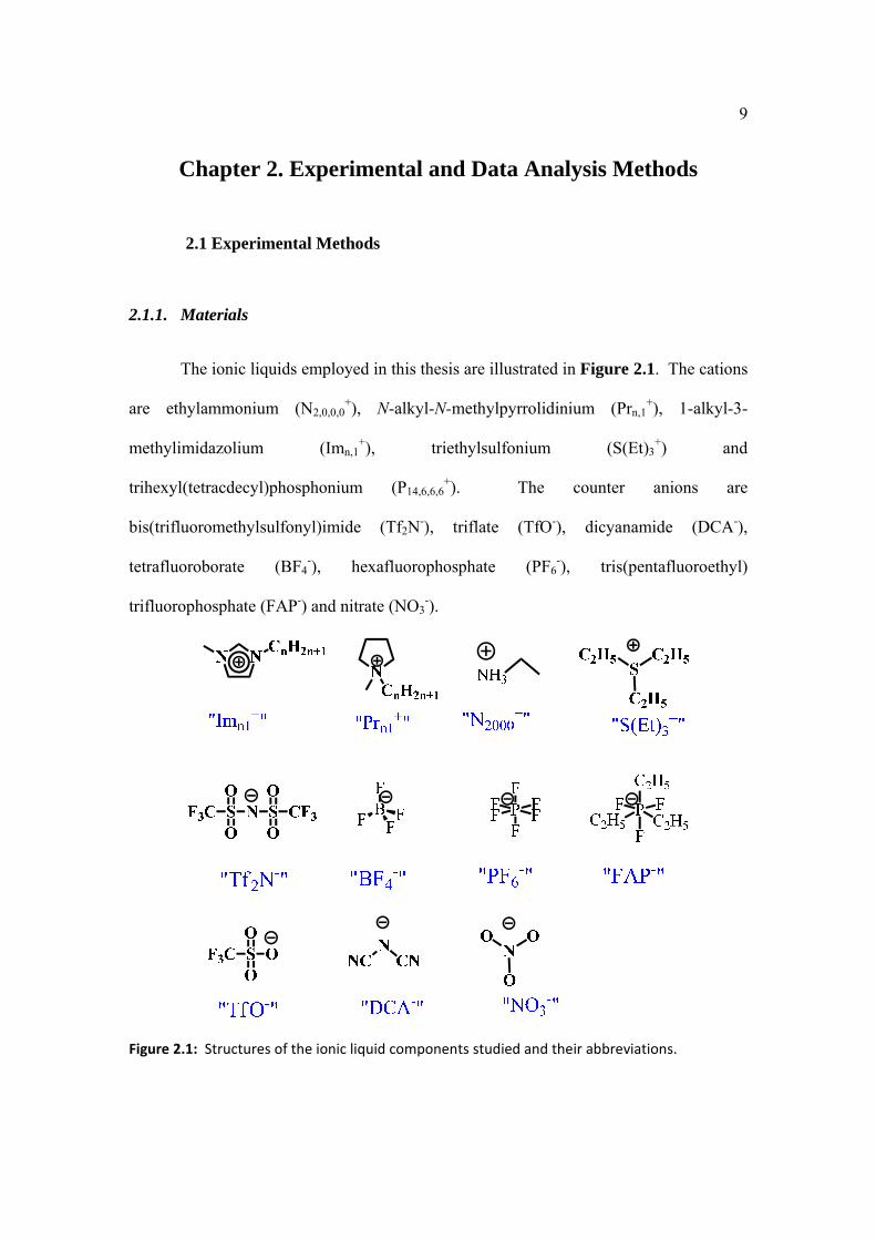
The ionic liquids employed in this thesis are illustrated in Figure 2.1. The cations
are ethylammonium (N2,0,0,0+), N-alkyl-N-methylpyrrolidinium (Prn,1
+), 1-alkyl-3-
methylimidazolium (Imn,1+), triethylsulfonium (S(Et)3
+) and
trihexyl(tetracdecyl)phosphonium (P14,6,6,6+). The counter anions are
bis(trifluoromethylsulfonyl)imide (Tf2N-), triflate (TfO-), dicyanamide (DCA-),
tetrafluoroborate (BF4-), hexafluorophosphate (PF6
-), tris(pentafluoroethyl)
trifluorophosphate (FAP-) and nitrate (NO3-).
Figure 2.1: Structures of the ionic liquid components studied and their abbreviations.

10
The fluorophore, Coumarin 153 (C153, laser grade, Figure 2.2) was purchased
from Exciton and used as received. C153 is applied to study the solvation dynamics of
about 20 pure ionic liquids (Chapter 3) and the mixture [Im41][BF4] + acetonitrile
(Chapter 4). Figure 2.2 also shows the fluorophore and the quencher studied for
bimolecular electron transfer in Chapter 5. The fluorophore 9,10-dicyanoanthracene
(DCA) was selected because it does not undergo a dynamic Stokes shift, which simplifies
the observation of “dynamic” quenching. DCA is also chosen due to its long lifetime, 13
ns. DCA was recrystallized from pyridine/acetonitrile.1 N,N-dimethylaniline (DMA,
redistilled, 99.5+%) was used as received from Aldrich.
Figure 2.2: Structures of probe coumarin 153 (C153), the electron acceptor (DCA) and donor (DMA).
All of the ionic liquids studied were dried under vacuum at 45 °C overnight prior
to measurement. The water contents of samples were measured using a Mettler-Toledo
DL39 Karl Fischer coulometer, and were below 100 ppm by weight prior to use for most
ionic liquids in this study.

11
The viscosities of most pure ILs (Chapter 3) were measured with a Brookfield
Model HBDV-III+CP cone/plate viscometer. The viscometer was calibrated using the
NIST-certified viscosity standards N75 and N100. In most cases, viscosities were
measured from 5 to 65 °C with an increment of 5°C. The Vogel-Fulcher-Tammann
(VFT)2 Equation (Eq. 2.1) was used to characterize these viscosity data.
KTT
BAcP
/)()/ln(
0
(2.1)
In this expression, is the liquid viscosity at temperature T, and A, B and T0 are fitting
parameters. The viscosities of the mixture [Im41][BF4] + acetonitrile (Chapter 4) were
measured at 20.5 °C using Cannon-Fenske Routine Viscometers (CFRV) of varying sizes
from model #50 (0.8-4 cSt) to #200 (20-100 cSt). At least three values were obtained for
each mixture.
2.1.2. Steady-State Measurements
Steady-state absorption spectra were measured using a Hitachi U-3000 UV/Vis
spectrometer at 1 nm resolution. Most absorption spectra were measured at room
temperature 21 2 °C. Steady-state fluorescence spectra were recorded with a SPEX
Fluorolog 212 spectrometer (2 nm resolution) at the desired temperature ( 0.1°C)
controlled using a circulating water bath. The emission correction file of the fluorometer
was made following the method described by Gardecki and Maroncelli.3 To obtain the
correction file, the emission spectra of six dyes covering the range 310-840 nm were
measured and the normalized spectra compared to standard emission spectra.3 Quartz
cuvettes with 1 cm light path were used for the absorption and right-angle steady-state

12
emission measurements. The optical densities of the fluorescence samples were kept
around 0.1 O.D. To reduce the effects of impurity emission, front-face geometry
emission measurements were performed in ILs which had relatively high fluorescence
backgrounds. Quartz cuvettes with 1 mm light path were used for the absorption and
front-face steady-state emission measurements. For those measurements, the optical
densities of the samples were kept around 1. The emission spectra of C153 in [Im41][BF4]
were measured under both right-angle and front-face conditions to check the reliability of
the front-face experiment. Except for temperature-dependent measurements, all of the
solvation dynamics measurements in Chapter 3 and 4 were maintained at 20.5 0.1°C
due to the limited temperature control of the fluorescence up-conversion system, while
the bimolecular electron transfer in Chapter 5 was studied at 25.0 0.1°C.
2.1.3. Time- Correlated Single Photon Counting Measurements
The time-resolved fluorescence data were recorded using a home-built time-
correlated single photon counting (TCSPC) setup. Figure 2.3 shows a schematic of the
TCSPC instrument.4 As shown in this illustration, the fundamental laser pulse
(700~1000 nm) was generated by a cavity-dumped Ti:sapphire laser, which was doubled
by a BBO crystal. The frequency-doubled pulse excited the sample after travelling
through a polarizer that only transmits vertical light. With the exception of anisotropy
experiments, fluorescence decays were collected at the magic angle (54.7) with respect
to the excitation to eliminate the effects of solute rotation. A scattering solution was used
to determine the instrumental response function. In all of the TCSPC experiments
discussed here the instrument response function had a width of ~25 ps (full width at half

13
maximum). The typical time window for data collection was about three times the
fluorophore lifetime. All decays were fit to multi-exponential functions using a
convolute-and-compare algorithm (see Section 2.2.2).
1. Figure 2.3: Time‐correlated single photon counting setup. M: Mirror. BS: beam splitter. PD:
photodiode. λ/2: half‐wave plate. FL: focus lens. BBO: beta barium borate (‐BaB2O4). PL:
polarizer. MCP‐PMT: microchannel plate photomultiplier tube. TAC: time‐to‐amplitude
converter. MCA: multichannel analyzer.

14
2.1.4. Fluorescence Up-Conversion Measurements
3.
Figure 2.4:5 Schematic of the broadband Fluorescence UP‐conversion Spectrometer (FLUPS). KDP II, 2‐mm‐thick frequency‐doubling KDP crystal; Pr1, Pr2, Pr3, SF59 prisms; M1, M5, plane mirrors; M2,M3,M4,M6, spherical mirrors; L1,L2,L3,L4,L5, BK7 lenses; P1, P2, polarizers.
A broadband fluorescence upconversion spectrometer (FLUPS) with femtosecond
time-resolution5,6 was applied to measure fast solvation dynamics by our collaborators,
Xinxing Zhang and Prof. Nikolaus Ernsting from Humboldt University of Berlin. Figure
2.4 shows a schematic of the FLUPS measurement. A Ti:sapphire laser (FEMTOLASERS
sPro) generates 500 μJ pulses at 800 nm a 500 Hz repetition rate. This fundamental laser
pulse is then split into two beams. One part was used as gating pulse which was
generated by a traveling-wave optical parametric amplifier of superfluorescence (TOPAS,
LIGHTCONVERSION). The other portion was frequency doubled to 400 nm pulses with 40
fs FWHM after compression and used as the optical pump. This beam was attenuated (~
1 µJ) and focused onto the sample by a thin lens (fl = 200 mm, fused silica) to a spot
diameter of 0.1 mm. The sum frequency signal was then generated by focusing the
Gate, 1340nm, 60 J
Pump, 400nm1 J, 40fs
KDP II
Time Delay
Sample Cell
P2
P1
M1
M2
M3
M4
L2
L3 M6
Pr1 Pr2
Pr3
A
20
L1
Fiber Bundle
L4 L5

15
delayed fluorescence and gating pulse into a potassium dihydrogen phosphate (KDP)
crystal. The sample cell was kept in a sealed flowing argon environment consisting of a
glass chamber with P2O5 desiccant. The water fraction could typically be maintained to
lower than 200 ppm by weight using this setup. FLUPS measurements were performed
at room temperature, 20.5 1 C.
2.1.5. Diffusion Measurements
Diffusion coefficients reported in Chapter 4 and 5 were measured by Anne Kaintz
in the Maroncelli group. These measurements employed 1H data measured on Bruker
DRX-400 and AV-III-850 spectrometers using the longitudinal eddy current delay
stimulated echo pulse sequence with bipolar gradient pulses.7 Diffusion coefficients D
were then calculated according to Equation 2.2.
22exp 222
0
gDI
I (2.2)
where Io is the initial peak intensity, γ the gyro-magnetic ratio of the nucleus, δ the
gradient pulse duration, g the gradient amplitude, ∆ the time between gradient pulse pairs,
and τ the time allowed for gradient recovery before the next pulse.

16
2.2.Data Analysis Methods
2.2.1. Deconvolution of TCSPC Decays
To obtain the highest effective time resolution from TCSPC, deconvolution is
used to partially remove the effects of the finite time resolution of the experimental setup.
To do so, an appropriate instrument response function, R(t) which depends on the
characteristics of both the detector and the timing electronics, is needed. We determine
R(t) experimentally by the response observed from a scattering solution. The measured
fluorescence decay IM (t) is a convolution of the ideal “real” decay IR(t) and the
instrument response function using the following equation,8
t
RM dttRttItI0
')'()'()( (2.3)
This convolution means that the measured emission intensity at time t is a weighted sum
of all the emission between time zero and that time.
A nonlinear least squares (NLLS) data processing method is then applied to fit the
ideal decay to some assumed functional form. The goal of a least square analysis is to fit
the data and test whether the chosen mathematical method is consistent with the real data
points. The least square analysis is applicable if the data satisfies certain assumptions.
The main assumptions are that there is a sufficient number of independent data points, the
uncertainties are Gaussian distributed and there is no systematic error.8 For TCSPC
measurements of bulk samples, these requirements are usually satisfied. The next step is
getting the fitting parameters from an appropriate mathematical model. The value of χ2,

17
the goodness-of-fit parameter, is used to determine whether the mathematical model is
consistent with the data or not. χ2 is given by the following equation,8
2
12
2 )]()([1
kCkM
n
k k
tItI
(2.4)
where k is the standard deviation of each data point k, n is the number of data points and
IC(tk) represents the calculated decay using the fitting parameters. For TCSPC data, it is
easy to define the standard deviation, k , which is the square root of the number of
photon counts in a given channel k based on Poisson statistics.8 The minimization of χ2
gives us the best fitting parameters within the chosen mathematical model. The value of
χ2 will be bigger for a larger data set, so we used the reduced χ2 for our TCSPC data
analysis,
pnR
2
2 (2.5)
where p is the number of the variable parameters in the model. For TCSPC, the number
of data points, n, is much larger than the number of variable parameters; therefore χR2 is
approximately equal to χ2 / n. χR2 is expected to be unity when there are no systematic
errors present in the data and the mathematical model is appropriate.8 Typically, TCSPC
data are fit to multi-exponential functions until the value of χR2 falls in the range 0.8-1.2.
Figure 2.5 shows a typical instrumental response function (black), observed fluorescence
decay (red) and the fitted fluorescence decay (blue).

18
Time / ps0 5000 10000 15000 20000
Rel
ativ
e In
tens
ity
0
0
1
10
100
1000
10000
Instrumental response funcitonObserved fluorescence decayFitted fluorescence decay
Figure 2.5: Representative experimental data, instrumental response function (black), observed fluorescence decay (red) and the fitted (blue) decay.
2.2.2. Reconstruction and Fitting of Time-Resolved Spectra
To obtain time-resolved spectra from TCSPC, about twenty time-resolved
emission decays were recorded at different wavelengths across the steady-state emission
spectrum. The measured TCSPC emission intensity decays at specific wavelengths (λj)
are fit to a multi-exponential function,8
i ji
jij
taItI ]
)(exp[)();( 0
with 1)( jia (2.6)

19
providing );( jtI at 20 different wavelengths, all represented by multi-exponential
functions. These parameterized data are then normalized based on the steady-state
fluorescence spectrum FSS (λ), using the fact that FSS (λ) at any λ is proportional to the
time integral over );( tI . The normalization equation used to obtain the reconstructed
time-resolved spectrum is 9
T
flii
iSSii
TIdttI
FtItF
0
);();(
)();();(
(2.7)
where τfl is the fluorescence lifetime and T is the time at the end of data collection
window. (The second part of the denominator in Equation 2.7, is obtained by integrating
);( itI from T to infinity.) Figure 2.6 shows representative time-resolved spectra
obtained in this manner. Also shown is the estimated time-zero spectrum discussed in
Section 2.2.3. The frequency base spectra are converted from wavelength dependent
spectra in the manner2
.
The spectra obtained by reconstruction are characterized by fitting the spectrum at
any time to a log-normal line shape function:9
}]
)1ln([2lnexp{);( 2
htvF (with the requirement of > -1) (2.8)
where
)(2 pvv , h the peak height, γ the asymmetry parameter, vp the peak
frequency and a width parameter. The solid curves in Figure 2.6 are from such fitting.
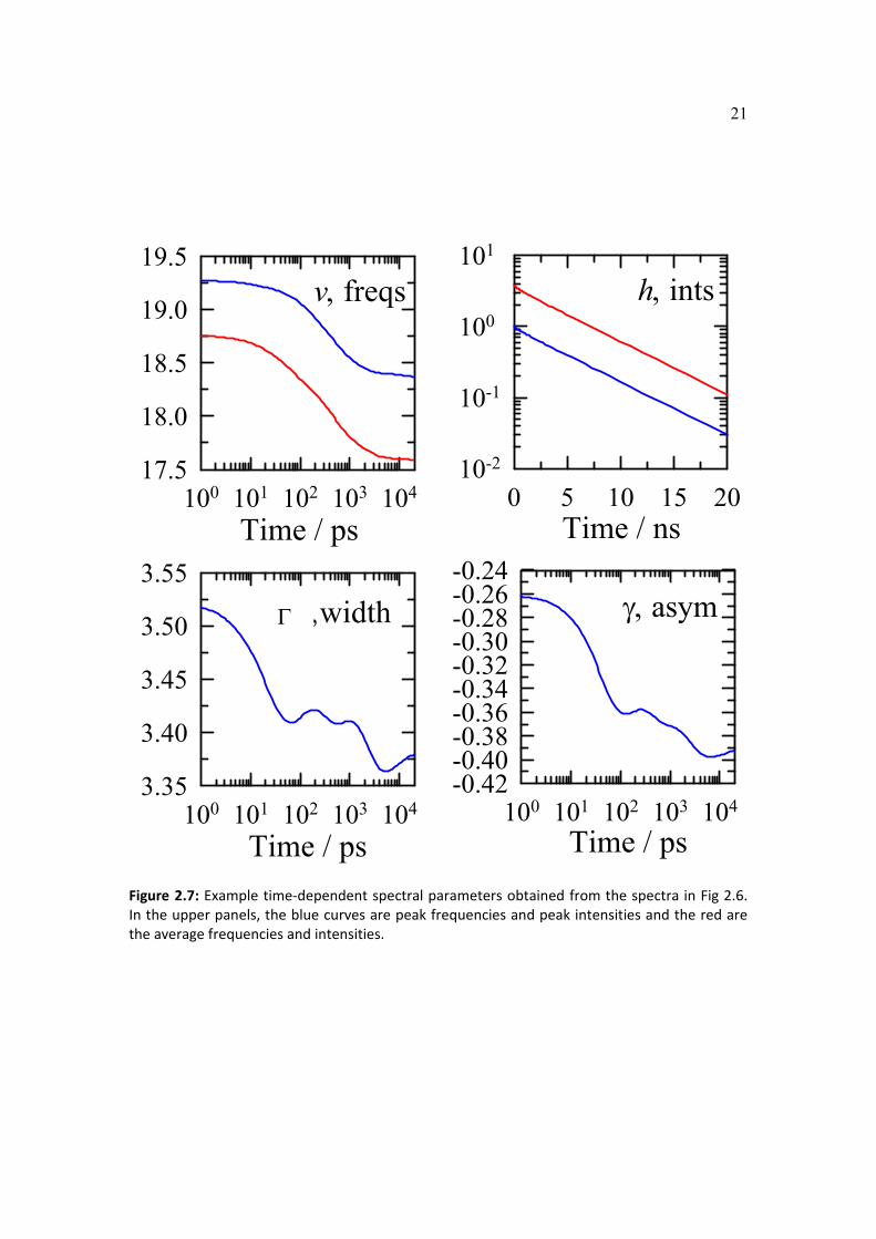
Figure 2.7 shows the time evolution of the fitting parameters from these spectra. In order
to calculate the solvation energy in the next section, both the peak frequency vp(t) and the
average (first moment) frequency va(t) of the spectrum

20
1
)2ln(4
)(3exp
)(2
)()()(
2t
t
ttvtv pa
(2.9)
are applied. Besides the frequencies, the time-dependent integrated intensity I(t) and the
full width at half-maximum )(t are also calculated using the following equations,
])2ln(4
)(exp[)()(]
)2ln(4[)(
22/1 t
tthtI
(2.10)
])(
))(sinh()[()(
t
ttt
(2.11)
Frequency / 103 cm-114 16 18 20 22 24
Rel
ativ
e In
tens
ity
0.0
0.2
0.4
0.6
0.8
1.020 ps50 100200 500100050001000020000
Figure 2.6: The deconvoluted time‐resolved spectra of C153 in [Im41][BF4]. Dots are the original data points at different wavelengths and the solid lines are the fitted log‐normal functions. The dash line is the estimated time‐zero spectrum (see Section 2.2.3).
21
v freqs
Time / ps100 101 102 103 104
17.5
18.0
18.5
19.0
19.5h ints
Time / ns0 5 10 15 20
10-2
10-1
100
101
width
Time / ps100 101 102 103 104
3.35
3.40
3.45
3.50
3.55 asym
Time / ps100 101 102 103 104
-0.42-0.40-0.38-0.36-0.34-0.32-0.30-0.28-0.26-0.24
Figure 2.7: Example time‐dependent spectral parameters obtained from the spectra in Fig 2.6. In the upper panels, the blue curves are peak frequencies and peak intensities and the red are the average frequencies and intensities.

22
2.2.3. Solvation Dynamics Calculation and the Time-Zero Spectrum
To characterize the time-dependence of solution, the spectral response function,
)()0(
)()()(
vv
vtvtSv
(2.12)
is used. Equating S(t) to the solvation response assumes that there is no significant
interference from changes to vibronic structure. To determine S(t), v(0) and v() are
required. The following discussion describes how v(0) can be determined based on the
Fee-Maroncelli method10,11. While for v(t) and v(∞), the results from reconstruction of
time-resolved spectra are used.
The accuracy of the experimentally determined time-zero spectrum depends
strongly on the time resolution of the experimental setup. Fee and Maroncelli11 have
discussed the unreliability of time-zero spectra derived by the extrapolating observed
spectra back to zero time and described a method for estimating the time-zero spectrum
based on steady-state absorption and emission spectra. The basic idea of this method is
the assumption that prior to solvent relaxation the Stokes shift of a given fluorophore in a
polar solvent should be the same as its Stokes shift in a non-polar solvent. An
approximate time-zero frequency v(0) can be calculated as
)()()()0( absvemvabsvv npnppp (2.13)
where the subscripts “p” and “np” represent the polar solvent of interest and a reference
non-polar solvent, respectively. For the solvation dynamics of C153 in pure ILs (Chapter
3) and the mixture of the ionic liquid and polar solvent (Chapter 4), the absorption and
emission spectra of C153 in 2-methylbutane (Fig. 2.8) are used as the non-polar
references for determining the time-zero spectra.

23
Frequency / 103 cm-116 18 20 22 24 26 28
Rel
ativ
e In
tens
ity
0.0
.2
.4
.6
.8
1.0SS fl t0 fl ref
flrefabs
abs & fit
Figure 2.8: Representative steady‐state spectra. The spectra of absorption (black), emission (cyan), absorption from log‐normal fitting (green dash) and the estimated time‐zero (blue) spectra of C153 in [Im61][Tf2N]. Red dash curves are the reference emission and absorption spectra of C153 in 2‐methylbutane.
Equation 2.13 is just a simple approximate way to estimate the time-zero
frequency. A more accurate model of the inhomogeneous broadening in polar solvents
was introduced to provide a more accurate estimate by Fee, Milsom and Maroncelli.10
Assuming that there is a single line-shape function g(v) which represents the absorption
spectrum of all solutes to within some spectral shift , the inhomogeneously broadened
absorption spectrum of the solute in a polar solvent can be described by 11

24
dpvgvvA )()()( (2.14)
where A(v) represents the absorption spectrum and p(δ) is the equilibrium distribution of
spectral shifts. The latter function is assumed to be Gaussian 11
])(
2
1exp[)2()( 202/12
p (2.15)
where 0 describes the average spectral shift from the non-polar reference solvent to the
polar solvent and σ2 represents the variance of the distribution. The time-zero emission
spectrum observed with excitation vex can be described as,10
dkvfpvgvvvtvF radexexexp )()()()();0,( 3 (2.16)
where )(vf is the emission line-shape of the solute and krad represents the radiative rate
constant. To estimate the time-zero spectrum, four functions, )(),(),( vfpvg and )(radk
must be specified. The line-shapes )(vg and )(vf can be obtained from the absorption
Anp(v) and emission Fnp(v) spectra of the solute in a non-polar solvent via
)()( 1 vAvvg np
and )()( 3 vFvvf np (2.17)
Now we need to define )(radk since the site distribution function )(p has been
described in Equation 2.15. (The assumption was made that the non-radiative nrk is
independent of and all the dependence on the spectral shift is due to the radiative
decay rate )(radk .) Fee and coworkers10,11 assumed that the radiative rate only depends
on the 3v factor in the Einstein A coefficient. Thus, the radiative rate function )(radk is
calculated as
dvvf
dvvvfvkrad
)(
)()()(
3
3
(2.18)
25
It is worth mentioning that σ and δ are determined by fitting the absorption spectrum and
these values used for the emission calculation. The value of 2ln8 (also known as inh
) describes the inhomogeneous broadening of the observed spectra. After all four
functions )(),(),( vfpvg and krad() are obtained; they can be input into the Equation
2.16 to get the time-zero spectrum of the solution in a polar solvent. Figure 2.8 shows
representative time-zero estimated spectrum along with the raw absorption and emission
spectra.
2.2.4. Anisotropy Analysis
The origin of emission anisotropy is the directional character of the absorption
and emission of light. In an isotropic sample, fluorophore molecules are randomly
oriented prior to excitation. Those molecules whose transition moments are oriented
along the polarization direction (the electric vector) of the excitation pulse are
preferentially excited. The decay of the fluorescence anisotropy reveals the average
angular displacement of fluorophores that occurs between absorption and subsequent
emission.
Figure 2.98 illustrates the geometry of a typical anisotropy measurement. The
orientation of the emission polarization is defined by the electric vector of the excitation
pulse. I║ represents the emission intensity observed with parallel polarization and I┴
indicates the intensity of perpendicularly polarized emission. The ideal anisotropy, r(t),
is then defined as,

26
)(2)(
)()(
)(
)()(
tItI
tItI
totalI
differenceItr
(2.19)
The difference between parallel and perpendicular emission is normalized by the total
intensity, so the anisotropy is a dimensionless quantity and independent of the
fluorophore concentration as well as the total emission intensity.
Figure 2.9:8 A diagram of the fluorescence anisotropy measurement.
The objective is to measure the anisotropy without the influence of the
experimental setup. The real intensity ratio between the parallel and perpendicular
emission is different from the measured intensity by a factor of G, the relative sensitivity
of the detection system to these different polarizations.8 G varies with the emission
wavelength and the band pass of the monochromator. It can be determined by
HH
HV
H
V
I
I
S
SG (2.20)

27
where SV and SH are the experiment sensitivity at vertical and horizontal polarization, IHV
is the emission intensity at vertical polarization under the horizontally polarized
excitation and IHH is the emission intensity at horizontal polarization with horizontal
excitation. For our study, the G factor is calculated based on the ratio between
perpendicular and parallel intensity at long times which means that the time is long
enough that isotropy is reestablished in the sample. The measured anisotropy is then
calculated by the following equation12,13,
)(2)(
)()()(
tGItI
tGItItr
(2.21)
The time-resolved anisotropy r(t) can be fit to various functions. In general, r(t)
is fit to a stretched exponential function of time,
])(exp[)( 0
rot
trtr (2.22)
The average rotation time (<rot>) is calculated as
)1
(0 rot
rot r (2.23)
where r0 is the initial anisotropy which is the value in the absence of the depolarizing
process. )(x is the gamma function. For some fluorescence anisotropy decays (Chapter
4), two exponential functions are used to fit the anisotropy,
)]exp()exp([)(
22
110
ta
tartr (2.24)
The coorresponding average rotation time is
2211 aarot (2.25)
28
It is worth mentioning that the initial anisotropy value r0 can be measured using a frozen
sample in which the molecules do not rotate at all. Theoretically, the r0 value should be
within the range from -0.20 to 0.40 for any single-photon excitation. For this study, the
r0 value of 0.375 is applied to the C153 samples based on the Horng’s measurement of
C153 in a glassy solvent, propylene glycol at 200 K.13

29
Notes and References
(1) Morifumi Fujita, A. I., Tetsuro Majima, and Setsuo Takamuku. J. Phys.
Chem. 1996, 100, 5382.
(2) H. Vogel, P. Z., 645, 1921; G. S. Fulcher, J. Am. Ceram. Soc. 8, 339, 1925;
G. Tammann and W. Hesse, Z. Anorg. Allg. Chem. 156, 245, 1926.
(3) Gardecki, J. A.; Maroncelli, M. Applied Spectroscopy 1998, 52, 1179.
(4) Heitz, M. P.; Maroncelli, M. J. Phys. Chem. A 1997, 101, 5852.
(5) Zhang, X. X.; Wuerth, C.; Zhao, L.; Resch-Genger, U.; Ernsting, N. P.;
Sajadi, M. Rev. Sci. Instrum. 2011, 82, 063108/1.
(6) Zhao, L.; Luis Perez Lustres, J.; Farztdinov, V.; Ernsting, N. P. Physical
Chemistry Chemical Physics 2005, 7, 1716.
(7) Wu, D.; Chen, A.; Johnson, C. S., Jr. Journal of Magnetic Resonance,
Series A 1995, 115, 260.
(8) Lakowicz, J. R. Principles of Fluorescence Spectroscopy, 3rd ed.;
Springer: New York, 2006.
(9) Horng, M. L.; Gardecki, J.; Papazyan, A.; Maroncelli, M. J. Phys. Chem.
1995, 99, 17311.
(10) Fee, R. S.; Milsom, J. A.; Maroncelli, M. J. Phys. Chem. 1991, 95, 5170.
(11) Fee, R. S.; Maroncelli, M. Chemical Physics 1994, 183, 235.
(12) Jin, H.; Baker, G. A.; Arzhantsev, S.; Dong, J.; Maroncelli, M. Journal of
Physical Chemistry B 2007, 117, 7291.
(13) Horng, M. L.; Gardecki, J. A.; Maroncelli, M. J. Phys. Chem. A 1997, 101,
1030.

30
Chapter 3. Solvation Dynamics of Neat Ionic Liquids
3.1.Introduction
Studies of Ionic liquids (ILs) have been engendered by their numerous potential
applications. ILs have variety outstanding properties, like the low volatility, intrinsic
conductivity, and tailorabiliy. Compared to conventional organic solvents, those
significant advantages make ILs good candidates for fuel cells,1 electrolytes for
batteries2,3 and dye-sensitized solar cells4. ILs are also excellent solvents for synthesis.5
The emergence of ionic liquids as a new type of solvent environment and the
aforementioned potential applications has regenerated interest in solvation dynamics.6,7
Solvation dynamics, the time-dependent response of a solvent to solute perturbations, is a
fundamental characteristic of liquid-phase dynamics, and it determines how fast chemical
reactions like electron or proton transfer processes couple to a solvent environment.8,9
What is the difference between solvation dynamics in ILs and conventional
dipolar solvents? Is our understanding of conventional solvents applicable to ionic
liquids? To answer these questions, the dynamic solvent response in 21 ionic liquids has
been determined experimentally. To discover the extent to which our understanding of
solvation in dipolar liquids is transferrable to ionic liquids, some well-known correlations
in conventional solvents are examined as is the applicability of dielectric continuum
models.
Early solvation dynamic studies10,11,12, mostly using picoseconds techniques,
showed that some part of the solvation response of ILs occurs over the time range 10-11-
31
10-8 s. This portion of the dynamics is now known to be directly correlated to solvent
viscosity. Another important component of the response occurs at shorter times than can
be detected by a time-correlated single photon counting (TCSPC) measurements which
has 20-90 ps time resolution. A few groups measured solvation dynamics in ionic liquids
with sufficient time resolution to observe this fast component.13-17 In the present work,
the technique of broadband femtosecond fluorescence upconversion spectroscopy
(FLUPS) with 80 fs time resolution18,19 has been introduced. The combination of both
TCSPC and FLUPS can capture the complete solvation response from 10-13 s to 10-8 s.
One aspect of the present study is to test whether a simple dielectric continuum
model is applicable for ionic liquid systems. Simple dielectric continuum models are
known to be able to predict the solvation response of conventional dipolar solvents with
good accuracy.20-24 In the fourteen ionic liquids whose dielectric data are available for
comparison,25-32 the predicted and observed solvation times are clearly related; however,
the predictions are found to systematically overestimate the rate of solvation. In most
cases, the predicted solvation is faster than the measured results by a factor of 2-5.
3.2.Experimental Methods
Coumarin 153 (laser grade) was obtained from Lambda Physik and Exciton and
used as received. The 21 ionic liquids surveyed in this work are listed in Table 3.1. The
majority of these liquids were the highest purity commercially available. Several liquids
were synthesized by Gary Baker, Richard Buchner or by us, and in these cases references
to the synthetic procedures are provided in the table.

32
Table 3.1: Ionic Liquids Studied
# represents the ID and “IL” the structure abbreviations of ionic liquids used in this Chapter. “CAS RNs” indicate the CAS registration numbers. “OD” shows the optical density of the neat ILs at 400 nm with 1 cm light path length. “*” = front-face measurement.
# IL CAS RN Chemical Name Source OD
21 [Im21][DCA]* 370865-89-7 1-ethyl-3-methylimidazolium dicyanamide Iolitec (>98%) 0.48
22 [Im21][BF4] 143314-16-3 1-ethyl-3-methylimidazolium tetrafluoroborate Iolitec (>98%) 0.22
24 [Im21][TfO] 145022-44-2 1-ethyl-3-methylimidazolium triflate Merck 0.13
I2 [Im21][Tf2N] 174899-82-2 1-ethyl-3-methylimidazolium bis(trifluoromethylsulfonyl)imide Iolitec (99%) 0.06
41 [Im41][DCA] 448245-52-1 1-butyl-3-methylimidazolium dicyanamide Richard Buchner37 0.07
42 [Im41][BF4] 174501-65-6 1-butyl-3-methylimidazolium tetrafluoroborate Iolitec (99%) 0.03
43 [Im41][PF6] 174501-64-5 1-butyl-3-methylimidazolium hexafluorophosphate Iolitec (99%) 0.11
44 [Im41][TfO]* 174899-66-2 1-butyl-3-methylimidazolium trifluoromethanesulfonate Iolitec (99%) 0.35
I4 [Im41][Tf2N] 174899-83-3 1-butyl-3-methylimidazolium bis(trifluoromethylsulfonyl)imide Kanto Chemical 0.02
46 [Im41][FAP]* 917762-91-5 1-butyl-3-methylimidazolium tris(pentafluoroethyl) trifluorophosphate EMD Chemicals (high purity) 0.41
I6 [Im61][Tf2N]* 382150-50-7 1-hexyl-3-methylimidazolium bis(triflluoromethylsulfonyl)imide Iolitec (99%) 0.38
I8 [Im81][Tf2N]* 178631-04-4 1-octyl-3-methylimidazolium bis(triflluoromethylsulfonyl)imide Iolitec (99%) 0.30
I0 [Im10,1][Tf2N]* 433337-23-6 1-decyl-3-methylimidazolium bis(trifluoromethylsulfonyl)imide Iolitec (>98%) 0.11
P3 [Pr31][Tf2N] 223437-05-6 1-propyl-1-methylpyrrolidinium bis(trifluoromethanesulfonyl)imide Gary Baker38,39 0.03
P4 [Pr41][Tf2N] 223437-11-4 1-butyl-1-methylpyrrolidinium bis(trifluoromethanesulfonyl)imide Gary Baker38,39 0.01
P5 [Pr51][Tf2N] 380497-17-6 1-pentyl-1-methylpyrrolidinium bis(trifluoromethanesulfonyl)imide Gary Baker38,39 0.05
P6 [Pr61][Tf2N] 380497-19-8 1-hexyl-1-methylpyrrolidinium bis(trifluoromethanesulfonyl)imide Gary Baker38,39 0.01
P8 [Pr81][Tf2N] 927021-43-0 1-octyl-1-methylpyrrolidinium bis(trifluoromethanesulfonyl)imide Gary Baker38,39 0.04
P0 [Pr10,1][Tf2N] 1003581-49-4 1-decyl-1-methylpyrrolidinium bis(trifluoromethanesulfonyl)imide Gary Baker38,39 0.01
M1 [N2000][NO3] 22113-86-6 ethylammonium nitrate this work 40 0.17
M2 [S222][Tf2N] 321746-49-0 triethylsulfonium bis(trifluoromethylsulfonyl)imide Iolitec (99%) 0.01

33
Apart from drying, the liquids were used as received except for [Im41][BF4] and
[Im41][PF6] which were treated with activated carbon to remove colored impurities. All
the ILs were dried in vacuum overnight at 45 C. The water contents of most ILs were
less than 100 ppm by weight prior to use.
Samples for steady-state and time-correlated single photon counting
measurements were made up in vials and then transferred to either 1 cm or 1 mm sealed
quartz cuvettes. Flowing solutions were used for fluorescence up-conversion. These
solutions were protected from water in a Perspex box flushed with argon and pumped
through a thin optical cell which can also be oscillated perpendicular to the beam
direction. With this arrangement, samples typically maintained water levels of < 200
ppm over the course of an experiment (approximately 5 hours). However, in the cases of
[Im21][BF4] and [Im41][DCA] final water contents were near 1000 ppm. We do not
anticipate that water even at this level will significantly alter the results reported here.
This assertion is supported by experiments with [Im21][BF4]. For this ionic liquid we
made 7 different runs having varying water contents between 650-5000 ppm but observed
no systematic differences as a function of water content. FLUPS and absorption
measurements were carried out at room temperature (20.5 0.5) ˚C. Steady-state
fluorescence and TCSPC measurements were performed in temperature controlled cells
(20.5 0.5) ˚C.
Steady-state and ps/ns time-resolved fluorescence measurements were performed
in the same manner detailed in Ref.35 The only difference was that for several of the
ionic liquids having significant impurity fluorescence (denoted with asterisks in Table 3.1)
1 mm cuvettes were used and emission collected in a front-face geometry. In these cases,

34
C153 concentrations providing ODs of near 1 were used in order to minimize the effect
of impurity fluorescence. Excitation at 400 nm for TCSPC measurements was supplied
by the doubled output of a cavity-dumped Ti:sapphire laser which delivers ~150 fs pulses
at 800 nm and a repetition rate of 5.4 MHz. Emission was collected though an ISA H10
monochromator with a bandpass of 8 nm. The overall response time of the TCSPC
instrument was 25-30 ps (FWHM), as measured using a scattering solution. Emission
decays were recorded at over 20 wavelengths spanning the emission spectrum and these
decays independently fit to a multi-exponential form using an iterative reconvolution
algorithm in order to partially remove the effects of instrumental broadening.
Reconstucted time-resolved spectra were obtained from these fitted decays according to
the methods described in Ref.36
Femtosecond time-resolved emission measurements were made using a home-
built broadband fluorescence upconversion spectrograph18,19 which supplies emission
spectra over the range 425-750 nm. The experiment is based on a Ti:sapphire laser
(Femtolasers sPro) which provides 30 fs, 300 μJ pulses at 800 nm and a 500 Hz repetition
rate. The output of this laser system is split into two beams with intensities in a ratio of
6:1. Pulses with 430 μJ energy drive an optical parametric amplifier (TOPAS, Light
Conversion) which delivers 60 μJ, 1340 nm pulses in horizontal polarization used for
optical gating. For optical pumping, the rest of the fundamental light is frequency
doubled to 400 nm pulses whose polarization is set with a half wave plate plate. After
passing a triple mirror on a variable delay stage, attenuated pump pulses (~ 1 µJ) are
focused by a thin lens onto the sample cell, to a spot diameter of about 0.1 mm. To
obtain a good optical image with the subsequent collection optics, the sample cell is made

35
with two 0.2 mm thick windows, which are typically spaced 0.2-0.3 mm apart.
Fluorescence was refocused by an off-axis Schwarzchild objective and collected by a
concave mirror onto a KDP crystal for upconversion. The procedures used for spectral
correction and evaluation are described in detail in Ref.19. The temporal response of the
FLUPS experiment is given by the FWHM ≈ 80 fs of the Gaussian fits of the time trace
of pump scatter from pure methanol.
3.3.Results and Discussion
3.3.1. Solvation Energies
As in our previous work,35 before examining solvation dynamics, we consider the
energetics of the S0S1 transition of C153 in different ionic liquids. The solvent
contributions to the free energy difference solvG and the reorganization energy solv
associated with the S0S1 transition of C153can be calculated from
0)]([2
1GvvhG abssol (3.1)
)]()0([2
1 vvhsol (3.2)
In these equations abs, (0), and () represent some measure of the frequency of the
absorption, “time-zero” emission, and fully equilibrated emission respectively, and G0
is the gas-phase energy difference, 296 kJ/mol.35 Peak frequencies used to calculate
these quantities are summarized in Table 3.2. The time-zero frequency (0) is an
approximation for the vibrationally equilibrated emission spectrum that would be

36
observed before any solvent relaxation. It is determined using steady-state spectra of
C153 in the nonpolar reference solvent 2-methylbutane as described in Ref.41 The
equilibrated emission frequency () is determined by extrapolating time-resolved
TCSPC data using a stretched exponential fit (see below). As can be seen from the data
in Table 3.2, this frequency is in all cases within 200 cm-1 to the red of the steady-state
emission frequency em. Values of solvG and solv in Table 3.2 were derived by
combining data from peak and first moment frequencies.
Table 3.2: Summary of C153 Fequencies and Energies
# IL Abs Pk SS Pk t(0) Pk t() Pk solG sol
103cm-1 103cm-1 103cm-1 103cm-1 kJ/mol-1 kJ/mol-1
21 [Im21][DCA] 23.27 18.29 20.37 18.29 47.2 12.7±0.9
22 [Im21][BF4] 23.64 18.24 20.68 18.25 45.2±1.4 14.9±1.2
24 [Im21][TfO] 23.53 18.39 20.59 18.38 45.4±1.1 13.8±0.9
I2 [Im21][Tf2N] 23.59 18.57 20.65 18.57 43.7±1.1 12.8±0.9
41 [Im41][DCA] 23.28 18.40 20.48 18.41 46.3±1.4 12.7±1.2
42 [Im41][BF4] 23.44 18.44 20.63 18.41 45.7±1.0 14.2±0.8
43 [Im41][PF6] 23.48 18.59 20.66 18.49 45.2±0.9 13.0±0.7
44 [Im41][TfO] 23.51 18.52 20.58 18.49 44.7±1.1 12.9±0.9
I4 [Im41][Tf2N] 23.51 18.65 20.68 18.62 43.7±0.8 11.7±0.6
46 [Im41][FAP] 23.56 18.85 20.62 18.80 43.5±1.1 12.1±0.9
I6 [Im61][Tf2N] 23.55 18.79 20.59 18.74 43.0±1.1 11.5±0.9
I8 [Im81][Tf2N] 23.57 18.92 20.61 18.82 42.2±1.1 11.0±0.9
I0 [Im10,1][Tf2N] 23.62 19.04 20.64 18.86 41.5±1.1 10.8±0.9
P3 [Pr31][Tf2N] 23.70 18.70 20.84 18.67 42.7±0.8 13.2±0.6
P4 [Pr41][Tf2N] 23.66 18.78 20.82 18.74 41.9±1.0 11.9±0.8
P5 [Pr51][Tf2N] 23.64 18.89 20.70 18.81 41.9±1.1 11.7±0.9
P6 [Pr61][Tf2N] 23.58 18.90 20.71 18.81 42.8±0.8 11.4±0.6
P8 [Pr81][Tf2N] 23.59 19.05 20.71 18.92 41.5±1.1 11.0±0.9
P0 [Pr10,1][Tf2N] 23.63 19.22 20.73 19.02 40.7±0.8 10.8±0.6
M1 [N2000][NO3] 22.98 18.24 20.44 18.25 49.3±2.2 13.0±1.8
M2 [S222][Tf2N] 23.63 18.63 20.68 18.61 43.1±1.1 12.7±0.9 Notes: “Abs Pk” represents the peak frequency of the steady state absorption spectrum. “SS Pk” is the peak frequency of the steady state emission spectrum.

37
Figure 3.1: Solvation contribution to the free energy change and reorganization energy
associated with the S0S1 transition of C153 versus mean ion separation, 3/1/1 mVd . Filled
symbols correspond to the data in Table 2 whereas open symbols are data on additional ionic liquids reported in Ref.35 Blue and cyan points are data in imidazolium ionic liquids (Im+), light green are pyrrolidinium (Pr+) and dark green ammonium ionic liquids (N+). Red points denote ionic liquids containing the trihexyltetredecylphosphonium cation and circles denote bis(trifluoromethanesulfonyl)imide ionic liquids. Lines are fits to all data excluding the
phosphonium liquids: dGsolv 1011.28 (N=30, r2=.80) and dsolv 594.3 (N=29,
r2=.59).
Free Energy s
olvG
/ kJ
mol
-1
40
42
44
46
48
50
52
ReorganizationEnergy
Å / d
0.08 0.10 0.12 0.14 0.16 0.18 0.20
sol
v / k
J m
ol-1
8
10
12
14
16
P14,666+Im+
Pr+
N+
Tf2N
-
othe
r
( )M1

38
Figure 3.1 shows these energies plotted versus the inverse of the mean ion
separation 3/1mVd where Vm is the molar volume. We use 1/d here as a coarse measure
of the strength of electrostatic interactions. This choice is based on the facts that the
lattice energy of the neat ionic liquid should scale with d-1 and also that the solvation
energy of ionic and dipolar solutes are inversely related to an effective cavity size,
2/~ dRRRa soluteionssolute . As illustrated in Fig. 3.1, variations in both solvG and
solv with ionic liquid appear to be reasonably correlated to this mean ion separation.
This observation and comparisons to conventional solvents were already discussed in our
previous work.35 The present study expands the original data set to 35 distinct ionic
liquids. As previously noted, ionic liquids based on the highly alkylated phosphonium
cation tetradecyltrihexylphoshonium (P14,666+) do not follow the same correlation as
established by the remaining ionic liquids (lines). The reorganization energy of protic
ionic liquid ethylammonium nitrate (“M1”) comprised of the smallest ions also seems to
deviate from the general trend. We also explored correlations of these energies which
incorporated the refractive index in an attempt to account for electronic polarizability,
which is expected to be relevant to solvG. But the refractive indices of the liquids
studied span a small range (1.43.03) and no improvement in the correlations was found.
The same can be said of the relative permittivities, r. Except for ethylammonium nitrate
(r = 28.30.542) , the relative permittivities available for 15 of the 21 liquids listed in
Table 3.2 all fall in a range characteristic of moderately polar conventional solvents r =
162.

39
3.3.2. Spectral / Solvation Response Functions
Figure 3.2: Time‐resolved emission spectra of C153 in [Pr51][Tf2N]. The top panel show FLUPS data (100 fs to 650 ps) and the middle panel spectra reconstructed from TCSPC decays (10 ps to 20 ns). The spike near 24,000 cm‐1 is due to Raman scattering. The smooth curves in both panels are fits of the data to log‐normal lineshape functions. The bottom panels compare the TCSPC and FLUPS spectra at two times.
16 18 20 22 24
Rel
ativ
e In
tens
ity 0.0
0.5
1.0
500 ps
16 18 20 22
0.0
0.5
1.0
200 ps
Frequency / 103 cm-116 18 20 22
0.0
0.5
1.0
0.1
650 ps
0.01
20 ns
FLUPS
TCSPC

40
Figure 3.2 shows representative time-resolved emission spectra in [Pr51][Tf2N].
In the top panel are broad-band spectra recorded using the FLUPS technique. In the
middle panel are spectra reconstructed from TCSPC decays (points). Both types of data
were fit with log-normal lineshape functions (smooth curves in both panels) in order to
parameterize the time evolution of the spectra.36 The bottom panel of Fig. 3.2 shows the
level of agreement typically observed between spectra obtained with FLUPS and TCSPC
over the time range where both spectra are expected to be reliable.
Figure 3.3 displays the behavior of two log-normal parameters derived from the
spectra in Fig. 3.2, the width (t) and the peak frequency pk(t). As illustrated in the top
panel of Fig. 3.3, we typically observe a substantial (~1000 cm-1) decrease in the width of
the spectrum at times of less than 100 ps. Recent work in conventional solvents
demonstrates that this width change is due primarily to vibrational cooling subsequent to
excitation with excess energy (~3000 cm-1).43 As has been done in past work, we will
ignore this effect and focus on the evolution of the peak frequency to monitor the
solvation response. Specifically, we will extract the spectral response function,
)()0(
)()()(
pkpk
pkpk ttS
(3.3)
and equate this frequency response to the solvation response, i.e. the normalized function
describing relaxation of the solute-solvent interaction energy. The solvation response
functions obtained in this manner will be contaminated to some degree by the vibrational
effect, but we anticipate that the distortions will not be greater than other sources of
uncertainty in the data.

41
Figure 3.3: Illustration of the combination of FLUPS and TCSPC. Time evolution of the spectral
width (FWHM; (t)) and peak frequency pk(t) obtained from log‐normal fits of the FLUPS and TCSPC spectra in Fig. 3.2. (See text.)
Full Width
3.5
4.0
4.5
5.0
Peak Frequency
10-1 100 101 102 103 104
19.0
19.5
20.0
20.5
21.0
pk /
103 c
m-1 +.23
shift
Time / ps
TCSPC
FLUPS
/ 1
03 cm
-1
TCSPC
FLUPS
splice

42
As shown in the bottom panel of Fig. 3.3, the peak frequencies measured in the
FLUPS and TCSPC experiments are not in perfect agreement. In the case illustrated here,
there is a 230 cm-1 difference between the two frequencies over the time range, 100-600
ps, where we expect both methods to be reliable. These data are representative in that the
average absolute discrepancy is 270 cm-1 for the 21 data sets reported here. The sign of
the deviation is random (the signed average is 30 cm-1) and we attribute it to the
variability in the spectrum of the gating light used in the FLUPS experiments. Because
the TCSPC data are referenced to calibrated steady-state spectra we take the TCSPC
frequencies as being correct and shift the FLUPS spectra to best match over the 100-600
ps range. To smoothly splice together the two sets of data, we take a weighted average of
the shifted FLUPS and TCSPC frequencies such that the FLUPS data are given 100%
weight at 100 ps and the TCSPC data 100% weight at 600 ps, as shown in Fig. 3.3.
Composite pk(t) data generated in this fashion are shown in Fig. 3.4 for the
homologous series of ionic liquids [Imn1][Tf2N] and [Prn1][Tf2N]. Given that one expects
systematic behavior as a function of alkyl chain length n in such series, these data provide
some indication of the uncertainties in the pk(t) data. At times greater than 10 ps
systematic behavior is observed in both series. There is an orderly progression of the
limiting frequencies pk() and between 100 ps – 1 ns the pk(t) parallel one another to
better than 100 cm-1. (As will be seen shortly this parallelism indicates a common
stretched-exponential time dependence throughout these series.) At times below 1 ps the
data are not as orderly and below 300 fs the various curves cross in unexpected ways.

43
Figure 3.4: Time evolution of the peak frequencies pk(t) of C153 in the imidazolium [Imn1][Tf2N] and pyrrolidinium [Prn1][Tf2N] series of ionic liquids.
[Prn1][Tf2N]
Time / ps
10-1 100 101 102 103 104
Fre
quen
cy
pk( t
) / 1
03 cm
-1
18.5
19.0
19.5
20.0
20.5
21.0
21.5
3456810
[Imn1][Tf2N]
18.5
19.0
19.5
20.0
20.5
21.0246810
n
n

44
In the case of the [Imn1][Tf2N] series it is only the n=4 data that appears to
misbehave whereas in the [Prn1][Tf2N] series the data are randomly ordered at 100 fs.
We interpret these observations as indicating uncertainties in the pk(t) data to be roughly
100 cm-1 at times greater than 1 ps and as large as 400 cm-1 at 100 fs. With Stokes
shift magnitudes of ~2000 cm-1 these uncertainties translate into uncertainties in S(t) of
5% at most times and up to 20% at sub-picosecond times. Due to the large uncertainty
in some early time data, for converting p(t) data to spectral response functions, we used
the values of pk(0) obtained from steady-state estimates as described in Section 2.2.3. In
the majority of the data sets (16/21 cases) the mean absolute deviation of pk(t=50 fs)
from the estimated pk(0) was 170 cm-1 (8% of the predicted Stokes shift). In most of
these cases the observed frequency was slightly less than that predicted, as would be
expected based on the finite time resolution of the experiment. However in the
[Prn1][Tf2N] series for n>3 (5 data sets) the observed frequencies at early time exceeded
the time-zero estimates by an average of nearly 600 cm-1 (29%). The reasons for the
large discrepancies in these particular solvents are not known.
Representative spectral/solvation response functions S(t) are provided in Fig. 3.5.
As is clear from this figure and from the previous pk(t) plots, the solvation response is
strongly bimodal, consisting of a sub-picosecond component followed by another
component that extends from a few picoseconds out to nanosecond times. A convenient
way of characterizing these two components of the response is through fits of the S(t)
data to a Gaussian + stretched exponential form
})/(exp{)1(}exp{)( 2221
tftftS GGG (3.4)

45
Figure 3.5: Representative spectral response functions (points) and fits to Eq. 3.4 (solid curves).
Example fits are shown as the smooth curves in Fig. 3.5. In all cases, this simple
functional form suffices to represent the observed data to within anticipated
uncertainties.44 Table 3.3 summarizes the fit parameters for all of the ionic liquids
studied here. Also listed in Table 3.3 under the heading “Q” is a rough assessment of the
relative quality of the data sets based on the frequency shift required to match the FLUPS
an TCSPC data, the similarity of the data in the splicing region, and the level of
agreement between observed and predicted time-zero frequencies. Q=1 represents the
most reliable data.
[Im10,1][Tf2N][Im41][PF6][Im41][DCA][Im21][BF4]
Time / ps
10-1 100 101 102 103 104
Spe
ctra
l Res
pons
e S
(t)
0.0
0.2
0.4
0.6
0.8
1.0

46
Table 3.3: Parameterization of Spectral Response Data
# IL Q fG G <>G <>str ps-1 ps ns ns
21 [Im21][DCA] 1 0.180.08 142.8 0.09 0.01 0.34 0.0510.010 22 [Im21][BF4] 1 0.450.08 6.7 0.19 0.05 0.40 0.16±0.03
24 [Im21][TfO] 1 0.390.08 7.8±1.6 0.16 0.20 0.41 0.61±0.12
I2 [Im21][Tf2N] 2 0.250.08 6.2±1.2 0.20 0.06 0.44 0.15±0.04
41 [Im41][DCA] 1 0.270.08 12±2.5 0.10 0.04 0.40 0.12±0.02
42 [Im41][BF4] 2 0.340.08 7.0±1.4 0.18 0.17 0.48 0.37±0.11
43 [Im41][PF6] 1 0.330.08 5.8±1.2 0.22 0.45 0.50 0.90±0.18 44 [Im41][TfO] 2 0.370.08 6.7±1.3 0.19 0.24 0.50 0.48±0.14 I4 [Im41][Tf2N] 3 0.390.15 4.1±1.6 0.31 0.19 0.60 0.29±0.12 46 [Im41][FAP] 1 0.210.08 2.8±0.6 0.44 0.23 0.51 0.44±0.09 I6 [Im61][Tf2N] 3 0.220.08 4.7±0.9 0.27 0.25 0.55 0.41±0.17 I8 [Im81][Tf2N] 2 0.130.11 3.1±0.9 0.41 0.40 0.52 0.76±0.23 I0 [Im10,1][Tf2N] 1 0.110.08 3.4±0.7 0.37 0.55 0.49 1.13±0.23 P3 [Pr31][Tf2N] 1 0.320.08 3.9±0.8 0.32 0.14 0.49 0.29±0.06 P4 [Pr41][Tf2N] 2 0.330.11 3.3±1.0 0.38 0.21 0.54 0.37±0.11 P5 [Pr51][Tf2N] 2 0.290.15 2.3±0.9 0.55 0.31 0.56 0.51±0.15 P6 [Pr61][Tf2N] 2 0.320.15 2.8±1.1 0.45 0.42 0.58 0.66±0.20 P8 [Pr81][Tf2N] 3 0.220.15 3.4±1.4 0.37 0.59 0.56 0.98±0.39 P0 [Pr10,1][Tf2N] 3 0.160.15 1.1±0.4 1.16 0.82 0.53 1.49±0.60 M1 [N2000][NO3] 1 0.390.08 8.1±1.6 0.16 0.03 0.45 0.062±0.012
M2 [S222][Tf2N] 2 0.280.11 3.0±0.9 0.42 0.07 0.54 0.13±0.04 Notes: “Q” represents the quality of the experimental results. 1=very good, 2=good, 3=poor. Fitting parameters for Sv(t) are from the Gaussian + stretched exponential form Eq. 3.4.
Before discussing the fit parameters some comment is necessary concerning the
values of G obtained here. We have not attempted to deconvolute the FLUPS data in
order to try to eliminate the effects of the 80 fs (FWHM) instrumental response function
(IRF). This IRF width corresponds to a Gaussian frequency of -1ps 7.8IRF and one
might anticipate that observed values of G near to IRF would be significantly reduced
from their true values by instrumental broadening. Assuming both the fast response and

47
the IRF to be Gaussian functions of time, one would expect 222 IRFtrueobs so that
values of G > IRF would not be observed. But, as seen from Table 3.3, we do find G >
IRF in a number of cases. The reason is that we use an independent means of
establishing pk(0), which forces the fit of S(t) to account in approximate way for the
shortfalls in pk(t0) caused by instrumental broadening. This approach appears to
provide the best means of extracting short-time information from the current data and we
believe that the fitted values of G reported in Table 3.3 should provide reasonable
estimates even for G > IRF. Comparison to data with much higher time resolution
discussed later supports this claim.
We examined the extent to which the parameters fG, G, tG(1/e)teG, , and str
correlate with various properties of the ions or bulk liquids. The times teG and str are
respectively the 1/e time associated with the Gaussian component and the integral time of
the stretched exponential component, given by Ge
G et /)2( 2/11)/1( and
/)( 1 str . The ion properties examine included the cation (C) an anion (A)
masses and van der Waals radii, RC and RA, the reduced mass of a C+A pair, , and the
“inertial factor” 2/12/3)( AC RR introduced in Ref.14 Bulk liquid properties tested were
the molar volume and viscosity.45 Only weak correlations were found between fG and
these quantities. Given the fact that estimated uncertainties in fG ( 0.1-.15) are a large
fraction of its range this result is not surprising. It is clear, however, that fG decreases
with increasing alkyl chain length n in the two series [Imn1][Tf2N] and [Prn1][Tf2N]. The
timescale of the subpicosecond component of the response, characterized by G or G
is most strongly correlated to the C+A reduced mass, anion mass, and the inertia factor.

48
Figure 3.6: Correlation of the Gaussian frequency G with the inverse of the reduced cation+anion reduced mass. Circles indicate ionic liquids with the Tf2N
‐ anion, other shapes are other anions. Red and green symbols are the [Imn1][Tf2N] and [Prn1][Tf2N] series, respectively, blue symbols are liquids with Imn1
+ cations and dark red symbols M1 and M2. Numbers indicate ionic liquids as listed in Table 3.1. The line is a linear fit to all of the data except M1 ([N2000][NO3]), 20 points correlation coefficient = 0.92.
As noted in previous work,14,46 without pointing to any particular solvation
mechanism, such correlations confirm the inertial character of this ultrafast component,
as predicted by numerous simulation studies.47 Figure 3.6 illustrates the best of these
correlations, between G and -1. The dashed line labeled “IRF” in this figure is a
reminder of the 80 fs instrumental response time of the FLUPS experiment. With the
exception of the data in ethylammonium nitrate (M1) which is excluded from the fit
Inverse Reduced Mass mu/0.00 0.01 0.02 0.03 0.04
Gau
ssia
n F
requ
ency
G /
ps-1
0
2
4
6
8
10
12
14
R=.92
IRF
21
41
M1
[Imn1][Tf2N][Prn1][Tf2N]
42 22

49
shown here, the correlation is quite good. This correlation would predict a much higher
Gaussian frequency for ethylammonium nitrate than what is observed. It is worth
mentioning that the predicted magnitude of the Stokes shift (or reorganization energy, Fig.
3.1) observed in this ionic liquid (M1) is also much smaller than expected relative to
other ILs. These two deviations are likely to be related and warrant further study.
Figure 3.7: Correlation of the integral time associated with the stretched exponential component with solvent viscosity. Circles indicate ionic liquids with the Tf2N
‐ anion, other symbols are other anions. Red and green symbols are the [Imn1][Tf2N] and [Prn1][Tf2N] series, respectively, blue symbols are liquids with Imn1
+ cations and dark red symbols M1 and M2. Numbers indicate ionic liquids as listed in Table 3.1. The line is the correlation
1.2/cP)1.8(ps/ str .
Viscosity / cP
10 100
Slo
w T
ime
str
/ ps
100
1000
[Imn1][Tf2N][Pr
n1][Tf2N]
24
42
43
21
M1

50
The slow component of the solvation response, measured by str, is most
strongly correlated to the solvent viscosity . Figure 3.7 displays this correlation, which
can be represented by a power law, p str with p=1.20.2. This type of near
proportionality of the integral solvation time to viscosity in a single ionic liquid versus
temperature and within collections of ionic liquids has been reported numerous times
previously.13,35 In the present case it appears to hold to within uncertainties for the two
homologous series [Imn1][Tf2N] and [Prn1][Tf2N] but with a number of outliers, most
notably [Im21][TfO] (“24”) and ethylammonium nitrate (“M1”). This relationship
between the time of the slow solvation component and viscosity presumably reflects the
fact that solvation is associated with structural relaxation of the solvent as found in
computer simulations.48 One additional relationship, not previously noted, can be found
in the data in Table 3.3. There is a fairly good correlation (R=-0.84) is observed between
the dispersity of the slow solvation component, represented by the stretching exponent ,
and the Gaussian frequency G. It is unclear whether there is any physical meaning to
this correlation or not.
3.3.3. Comparisons to Dielectric Continuum Predictions
We now examine to what extent one can use the dielectric dispersion data
recently collected on neat ionic liquids (see Table 3.4) as input to simple continuum
descriptions of solvation to predict the solvation response measured here with C153. The
model we employ assumes the solute to be a point dipole centered in a spherical cavity of
dielectric constant u=2, representing the solute polarizability, surrounded by a solvent

51
having the generalized dielectric response function )(ˆ . The calculations are essentially
the same as those described in Ref.14 and previous work.20 Normalized response
functions are determined using the expressions
)0(ˆ)(ˆ
}/)](ˆ)(ˆ{[)(
1
ppLtS p
dc (3.4)
up
pp
21)(ˆ1)(ˆ
)(ˆ
(3.5)
where 1pL denotes an inverse Laplace transform with respect to the variable ip 2 .
In contrast to Ref.14 where the contribution of conductivity was erroneously neglected,
the dielectric function used here is the generalized function,49
02
)(ˆ)(ˆi
(3.6)
This function describes the frequency dependence actually observed in dielectric
measurements, whereas )(ˆ , the remainder after the diverging conductivity contribution
is removed, is what is typically reported.29,50

52
Table 3.4: Dielectric Dispersion Data Used
# IL Freq. Range () nD ()-nD2 cond Label Diel. Ref. nD ref Cond Ref
S/m
21 [Im21][DCA] 100 MHz - 10 THz +OKE 11.0 2.5 1.510 0.2 B 30 51 52
22 [Im21][BF4] 100 MHz - 10 THz +OKE 15.9 1.94 1.411 -0.1 1.55 B 30 53 54
22 [Im21][BF4] 1 MHz - 20 GHz 13.6 6.7 1.411 4.7 1.52 N 31 31 31
24 [Im21][TfO] 500 MHz - 10 THz 17.7 2.12 1.432 0.1 0.98 B 55 53 52
I2 [Im21][Tf2N] 90 GHz 12.9 3.18 1.423 1.2 0.90 B 63 56 57
I2 [Im21][Tf2N] 1 MHz - 20 GHz 12.3 4.7 1.421 2.7 0.95 N 31 31 31
I2 [Im21][Tf2N] 20 GHz 12.3 3.23 1.423 1.2 0.83 W 25 56 25
41 [Im41][DCA] 100 MHz - 3 THz 11.3 2.13 1.509 -0.1 1.052 B1 29 58 54
41 [Im41][DCA] 100 MHz - 10 THz + OKE 12.3 2.36 1.509 0.1 1.052 B2 30 58 54
42 [Im41][BF4] 100 MHz - 3 THz 12.2 1.06 1.422 -1.0 0.35 B 29 47 54
42 [Im41][BF4] 1 MHz - 20 GHz 14.1 5.45 1.421 3.4 0.44 N 31 31 31
42 [Im41][BF4] 200 MHz-20 GHz 11.0 4.08 1.422 2.1 0.30 W 26 47 26
43 [Im41][PF6] 100 MHz - 3 THz 11.8 2.1 1.410 0.1 0.15 B 29 47 54
43 [Im41][PF6] 1 MHz - 20 GHz 14.1 4.8 1.407 2.8 0.165 N 31 31 31
43 [Im41][PF6] 40 MHz - 40 GHz 12.4 3.26 1.410 1.3 0.16 Y 32 47 32
44 [Im41][TfO] 100 MHz - 90 GHz 15.6 1.82 1.438 -0.2 0.29 B 63 59 54
I4 [Im41][Tf2N] 100 MHz - 90 GHz 12.9 2.23 1.427 0.2 0.39 B 63 56 57
I4 [Im41][Tf2N] 1 MHz - 20 GHz 13.7 4.25 1.426 2.2 0.42 N 31 31 31
I4 [Im41][Tf2N] 200 MHz-20 GHz 11.5 3.03 1.427 1.0 0.37 W 25 56 25
I4 [Im41][Tf2N] 40 MHz - 40 GHz 12.7 2.7 1.427 0.7 0.37 Y 32 56 25
I6 [Im61][Tf2N] 200 MHz - 89 GHz 12.7 2.58 1.430 0.5 0.22 B 60 56 57

53
I6 [Im61][Tf2N] 1 MHz - 20 GHz 14.1 4.8 1.430 2.8 0.226 N 31 31 31
I8 [Im81][Tf2N] 1 MHz - 20 GHz 16.8 3.72 1.432 1.7 0.14 N 31 31 31
P4 [Pr41][Tf2N] 200 MHz - 10 THz 12.1 2.33 1.423 0.3 0.26 B 63 39 27
P4 [Pr41][Tf2N] 200 MHz-20 GHz 11.7 2.42 1.423 0.4 0.26 W 27 39 27
M1 [N2000][NO3] 500 MHz - 12 THz 28.5 2.52 1.452 0.4 2.50 B 61 62 28
M1 [N2000][NO3] 10 MHz - 1 THz (wet) 26.4 3.2 1.452 1.1 2.50 K 28 62 28
M2 [S222][Tf2N] 100 MHz - 3 THz 14.7 2.2 1.426 0.2 0.512 B 63 Min 2012 27 (measured)
M2 [S222][Tf2N] 200 MHz-20 GHz 13.2 1.83 1.426 -0.2 0.711 W 27 Min 2012 27 (fit)

54
Dielectric relaxation data are currently available for 14 of the 21 ionic liquids
studied here. The data are primarily from the groups of Buchner29,30,55,60,61 and
Weingärtner,25-28 as summarized in Table 3.4. Listed in this table are frequency ranges
over which data were collected. The upper limit of this range has a significant impact on
the quality of the solvation dynamics predictions possible. To capture the majority of the
intramolecular nuclear dynamics of relevance to solvation, characterization of )(ˆ
should extend to the terahertz range. For only 9 of the solvents are such extended
frequency data available. As shown by the column labeled 2Dn in Table 3.4, in
the remaining cases, some portion of the dielectric spectrum is missed. Although the
fraction missed, )/()( 20
2DD nn , is typically <25%, this missing fraction has a large
impact on the short-time response and, if not accounted for, can also affect the long time
behavior of S(t).
Figure 3.8 illustrates the problem and our method of approximating this missing
contribution. In Fig. 3.8 we show dielectric data reported by four laboratories for the
ionic liquid [Im41][Tf2N].25,31,32,63 Panel (a) shows the functions as reported. Panel (b)
shows these same functions modified by the addition of a damped harmonic oscillator of
amplitude 2Dn , which is used to account for unobserved high-frequency
components of )(ˆ . The data of Buchner et al.63 is not modified in this fashion because
0 . We note that the data of Buchner et al.63 (“B”, blue), Nakamura and Shikata31
(“N”, red) and Daguenet et al.25 (“W”, green) are in good agreement over their region of
overlap, whereas the data of Mizoshiri et al.32 (“Y”, purple) is rather different between

55
100 MHz – 20 GHz. Of these four data sets, only the data of Buchner et al.63 extend to
the THz range necessary to reduce )( to close to its value 2Dn at optical frequencies.
Figure 3.8: Dielectric relaxation and calculated solvation response functions of [Im41][Tf2N]. (a)&(b): Dielectric permittivity ( )( , upper curves) and loss ( )( , lower curves) functions
calculated from the parameterizations provided in Refs.25,31,32,63 (The legend refers to references as coded in Table 3.4.) (c)&(d): Solvation response functions calculated on the basis of the dielectric data in panel (a) and (b). The inset tables show the average time (tav) in ps required to reach certain values of S(t), 0.7, 0.5, 0.3 and 0.1. The values labeled “x” shows the spread in values which is obtained using the different dielectric data as the ratio of maximum value over minimum value excluding the “Y” values (dashed curves).
(a)
Frequency / s-1
107 108 109 1010 1011 1012 1013
Re{(
)},
Im{
( )}
0
2
4
6
8
10
12
14
BNWY
(b)
107 108 109 1010 1011 1012 1013
(c)
Time / s10-13 10-12 10-11 10-10 10-9
Sol
vati
on R
espo
nse
S( t
)
0.0
0.2
0.4
0.6
0.8
1.0(d)
10-13 10-12 10-11 10-10 10-9
S tav x
0.7 4 21
0.5 14 5
0.3 52 2.4
0.1 270 1.3
S tav x
0.7 1 2.2
0.5 4 1.5
0.3 27 1.4
0.1 200 1.2
n2
+DHO

56
Figure 3.8 panel (c) shows the solvation response functions directly calculated
from aforementioned four dielectric parameterizations. Equations 3.4 and 3.5 predict the
short-time (t<10 ps) dynamics differ significantly as clearly shown in Figure 3.8 panel
(a). To account for the difference between and 2Dn , an effective high-frequency
component is included in Equation 3.7, in the form of a damped harmonic oscillator,
)(
)()(ˆ20
202
pp
np D , (3.7)
In Figure 3.8 panel (c) the dielectric functions as parameterized are used and in
panel (d) these functions are modified by the addition of this damped harmonic oscillator
(Eq. 3.7). The inset shows the average times required to reach certain value of S(t). av is
the average time of the three solvation response (“B”, “N” and “W”). “x”, the ratio of the
maximum value over the minimum value among those three predictions, represents the
spread in values. Obviously, the panel (d) has much better agreement. Therefore, the
effective high-frequency contribution is included for all the dielectric continuum
predictions.
Figure 3.9 illustrates six representative comparisons between the experimental
solvation response functions and the S(t) predicted by the dielectric continuum model.
The black curves are the measured solvation response functions and colored curves are
from the dielectric continuum predictions. The labels “B”, “N”, “W” and “Y” represent
the dielectric data sources defined in Table 3.4. In most cases the dielectric continuum
predictions are similar in shape to the observed S(t) functions, especially in the ps~ns
time range. [Im21][TfO] is an extreme case where the predicted response is much faster
than the observed solvation response for reasons which are presently unclear.

57
[N2000
][NO3
]
B
W
Time / ps10-1 100 101 102 103 104
0.0
.2
.4
.6
.8
1.0
[Im21
][DCA]
B
0.0
.2
.4
.6
.8
1.0 [Im21
][BF4
]
B
N
[Im21
][TFO]
B
Sol
vati
on R
espo
nse
S(t)
0.0
.2
.4
.6
.8
1.0 [Im41
][PF6
]
B
N
Y
[SEt3
][Tf2
N]
B
W
10-1 100 101 102 103 104
Figure 3.9: Comparison of measured C153 spectra response functions (black curves) with dielectric continuum model predictions (colored curves). The legend with color to each plot indicates the source of the dielectric data (see Table 3.4.).

58
Figure 3.10 shows the comparisons of times when the S(t) functions reach certain
values. For 14 ionic liquids which we have dielectric data (Table 3.4), the times required
for S(t) predicted and observed to relax to four different values, 0.7, 0.5, 0.3, and 0.1 as
well the integral time <> are plotted. In general, the fast solvation dynamics are
indicated by the times when S(t) reaches levels of 0.7 and 0.5, while the 0.3 and 0.1 times
characterize the slower components of the solvation response. As illustrated in Fig. 3.10,
the predicted solvation response is faster than the observed response roughly by a factor
between 2 and 10.
Pred vs. Exp
Predicted Time / ps.1 1 10 100 1000
Obs
erve
d T
ime
/ ps
.1
1
10
100
1000
Time
S(t)
0.1
0.3
0.5
0.7
Figure 3.10: Comparison of the times required for predicted and observed S(t) at certain values of 0.7, 0.5, 0.3 and 0.1. The inset illustrates the meaning of the times when S(t) reaches certain values along with the color coding. The solid cyan symbols are the integral response times. The symbols with the diamond shape represent ILs with the Imn1
+ cation and M1. The circle symbols are ILs with the Tf2N
‐ anion.

59
3.4.Summary and Conclusions
The complete solvation response of coumarin 153 in 21 room-temperature ionic
liquids has been measured by combining broadband fluorescence upconversion and time-
correlated single photon counting. The combination of these two techniques provides
temporal coverage over times of 100 fs to 20 ns, which enables the observation of the
complete solvation response in a variety of ionic liquids. The fast solvation dynamics of
ionic liquids are correlated to the reduced mass of an ion pair. Such correlations confirm
the inertial character of this ultrafast component, as predicted by simulation results. The
slow solvation dynamics are correlated to the bulk viscosity, as has been observed
previously35. The measured solvation dynamics are then used to test the applicability of
simple dielectric continuum models to ionic liquids systems. The simple dielectric
continuum model provides a good starting point for predicting solvation dynamics in
ionic liquids, but the predicted dynamics are systematically faster than experiment.

60
Notes and Refrerences:
(1) Armand, M.; Endres, F.; MacFarlane, D. R.; Ohno, H.; Scrosati, B. Nat.
Mater. 2009, 8, 621.
(2) Plechkova, N. V.; Seddon, K. R. Chem. Soc. Rev. 2008, 37, 123.
(3) Frackowiak, E.; Lota, G.; Pernak, J. Appl. Phys. Lett. 2005, 86, 164104/1.
(4) Lewandowski, A.; Swiderska, A. Applied Physics A: Materials Science &
Processing 2006, 82, 579.
(5) Ionic Liquids in Synthesis; Wasserscheid, P.; Welton, T., Eds.; Wiley-
VCH: Weinheim, 2003.
(6) Samanta, A. Journal of Physical Chemistry B 2006, 110, 13704.
(7) Samanta, A. Journal of Physical Chemistry Letters 2010, 1, 1557.
(8) Li, X.; Liang, M.; Chakraborty, A.; Kondo, M.; Maroncelli, M. Journal of
Physical Chemistry B 2011, in press.
(9) Castner, E. W., Jr.; Margulis, C. J.; Maroncelli, M.; Wishart James, F.
Annual Reviews of Physical Chemistry 2011, 62, 85.
(10) Karmakar, R.; Samanta, A. Journal of Physical Chemistry A 2002, 106,
4447.
(11) Bart, E.; Meltsin, A.; Huppert, D. Chemical Physics Letters 1992, 200,
592.
(12) Ingram, J. A.; Moog, R. S.; Ito, N.; Biswas, R.; Maroncelli, M. Journal of
Physical Chemistry B 2003, 107, 5926.
(13) Arzhantsev, S.; Jin, H.; Ito, N.; Maroncelli, M. Chemical Physics Letters
2006, 417, 524.
(14) Arzhantsev, S.; Jin, H.; Baker, G. A.; Maroncelli, M. J. Phys. Chem. B
2007, 111, 4978.
(15) Lang, B.; Angulo, G.; Vauthey, E. Journal of Physical Chemistry A 2006,
110, 7028.
(16) Halder, M.; Headley, L. S.; Mukherjee, P.; Song, X.; Petrich, J. W.
Journal of Physical Chemistry A 2006, 110, 8623.

61
(17) Kimura, Y.; Fukuda, M.; Suda, K.; Terazima, M. The Journal of Physical
Chemistry B 2010, 114, 11847.
(18) Zhao, L.; Luis Perez Lustres, J.; Farztdinov, V.; Ernsting, N. P. Physical
Chemistry Chemical Physics 2005, 7, 1716.
(19) Zhang, X.-X.; Wurth, C.; Zhao, L.; Resch-Genger, U.; Ernsting, N. P.;
Sajadi, M. Reviews of Scientific Instruments 2011, submitted.
(20) Horng, M. L.; Gardecki, J. A.; Papazyan, A.; Maroncelli, M. Journal of
Physical Chemistry 1995, 99, 17311.
(21) Maroncelli, M. Journal of Chemical Physics 1997, 106, 1545.
(22) Song, X.; Chandler, D. Journal of Chemical Physics 1998, 108, 2594.
(23) Ruthmann, J.; Kovalenko, S. A.; Ernsting, N. P.; Ouw, D. Journal of
Chemical Physics 1998, 109, 5466.
(24) Sajadi, M.; Obernhuber, T.; Kovalenko, S. A.; Mosquera, M.; Dick, B.;
Ernsting, N. P. The Journal of Physical Chemistry A 2009, 113, 44.
(25) Daguenet, C.; Dyson, P. J.; Krossing, I.; Oleinikova, A.; Slattery, J.;
Wakai, C.; Weingärtner, H. Journal of Physical Chemistry B 2006, 110, 12682.
(26) Schröder, C.; Wakai, C.; Weingärtner, H.; Steinhauser, O. Journal of
Chemical Physics 2007, 126, 84511.
(27) Weingartner, H.; Sasisanker, P.; Daguenet, C.; Dyson, P. J.; Krossing, I.;
Slattery, J. M.; Schubert, T. J. Phys. Chem. B 2007, 111, 4775.
(28) Krueger, M.; Bruendermann, E.; Funkner, S.; Weingaertner, H.; Havenith,
M. Journal of Chemical Physics 2010, 132, 101101/1.
(29) Stoppa, A.; Hunger, J.; Buchner, R.; Hefter, G.; Thoman, A.; Helm, H.
Journal of Physical Chemistry B 2008, 112, 4854.
(30) Turton, D. A.; Hunger, J.; Stoppa, A.; Hefter, G.; Thoman, A.; Walther,
M.; Buchner, R.; Wynne, K. Journal of the American Chemical Society 2009, 131,
11140.
(31) Nakamura, K.; Shikata, T. ChemPhysChem 2010, 11, 285.
(32) Mizoshiri, M.; Nagao, T.; Mizoguchi, Y.; Yao, M. Journal of Chemical
Physics 2010, 132, 164510/1.
(33) Shim, Y.; Kim, H. J. Journal of Physical Chemistry B 2008, 112, 11028.

62
(34) Song, X. J Chem Phys 2009, 131, 044503.
(35) Jin, H.; Baker, G. A.; Arzhantsev, S.; Dong, J.; Maroncelli, M. Journal of
Physical Chemistry B 2007, 117, 7291.
(36) Maroncelli, M.; Fleming, G. R. Journal of Chemical Physics 1987, 86,
6221.
(37) Fredlake, C. P.; Muldoon, M. J.; Aki, S. N. V. K.; Welton, T.; Brennecke,
J. F. Physical Chemistry Chemical Physics 2004, 6, 3280.
(38) Baker, S. N.; McCleskey, T. M.; Pandey, S.; Baker, G. A. Chemistry
Communications 2004, 940.
(39) Jin, H.; O'Hare, B.; Dong, J.; Arzhantsev, S.; Baker, G. A.; Wishart, J. F.;
Benesi, A.; Maroncelli, M. Journal of Physical Chemistry B 2008, 112, 81.
(40) Weingaertner, H.; Merkel, T.; Kaeshammer, S.; Schroer, W.; Wiegand, S.
Ber. Bunsen-Ges. Phys. Chem. 1993, 97, 970.
(41) Fee, R. S.; Maroncelli, M. Chemical Physics 1994, 183, 235.
(42) Huang, M.-M.; Jiang, Y.; Sasisanker, P.; Driver, G. W.; Weingartner, H.
Journal of Chemical & Engineering Data 2011, 56, 1494.
(43) Sajadi, M.; Ernsting, N. P. 2012, private communication.
(44) Slightly better fits could be achieved using a sum of four exponential
functions, but the characteristics of most interest, the amplitudes and integral times
associated with the sub-picosecond (represented by the Gaussian in Eq. 4) and the ps-ns
(stretched exponential) components were close to those obtained from Eq. 4. Given the
much greater simplicity and interpretability of Eq. 4, we prefer it for our purposes. We
note that this functional form has also recently been shown to provide a convenient
means of accurately representing most response functions observed in simulations of
model ionic liquids.48
(45) The various ion and liquid properties examined here are not independent
and significant correlations are expected among them. One surprise was observation of a
strong correlation between the C+A reduced mass and the molar volume of the liquid,
R=0.986 for these 21 assorted ionic liquids.
(46) Muramatsu, M.; Nagasawa, Y.; Miyasaka, H. The Journal of Physical
Chemistry A 2011, 115, 3886.
63
(47) Soriano, A. N.; Doma, B. T.; Li, M.-H. Journal of Chemical
Thermodynamics 2009, 41, 301.
(48) Roy, D.; Maroncelli, M. The Journal of Physical Chemistry B 2012,
submitted.
(49) Note that different authors employ different conventions for describing
)()()(ˆ i and the sign of the conductivity correction depends upon this
choice. Equation 7 is appropriate for the positive sign convention.
(50) Buchner, R.; Hefter, G. T.; May, P. M. Journal of Physical Chemistry A
1999, 103, 1.
(51) Froeba, A. P.; Kremer, H.; Leipertz, A. Journal of Physical Chemistry B
2008, 112, 12420.
(52) Yu, Y.-H.; Soriano, A. N.; Li, M.-H. Journal of Chemical
Thermodynamics 2009, 41, 103.
(53) Soriano, A. N.; Doma, B. T., Jr.; Li, M.-H. J. Taiwan Inst. Chem. Eng.
2010, 41, 115.
(54) Zech, O.; Stoppa, A.; Buchner, R.; Kunz, W. Journal of Chemical and
Engineering Data 2010, 55, 1774.
(55) Schroder, C.; Sonnleitner, T.; Buchner, R.; Steinhauser, O. Phys Chem
Chem Phys, 13, 12240.
(56) Tariq, M.; Forte, P. A. S.; Gomes, M. F. C.; Lopes, J. N. C.; Rebelo, L. P.
N. Journal of Chemical Thermodynamics 2009, 41, 790.
(57) Tokuda, H.; Hayamizu, K.; Ishii, K.; Susan, M. A. B. H.; Watanabe, M.
Journal of Physical Chemistry B 2005, 109, 6103.
(58) Seoane, R. G.; Corderi, S.; Gomez, E.; Calvar, N.; Gonzalez, E. J.;
Macedo, E. A.; Dominguez, A. Industrial and Engineering Chemistry Research 2012, 51,
2492.
(59) Anderson, J. L.; Armstrong, D. W.; Wei, G. T. Analytical Chemistry 2006,
78, 2893.
(60) Hunger, J.; Stoppa, A.; Schroedle, S.; Hefter, G.; Buchner, R.
ChemPhysChem 2009, 10, 723.

64
(61) Turton, D. A.; Sonnleitner, T.; Ortner, A.; Walther, M.; Hefter, G.;
Seddon, K. R.; Stana, S.; Plechkova, N. V.; Buchner, R.; Wynne, K. Faraday Discuss.
2012, 154, 145.
(62) Greaves, T. L.; Weerawardena, A.; Fong, C.; Krodkiewska, I.;
Drummond, C. J. Journal of Physical Chemistry B 2006, 110, 22479.
(63) Buchner, R. 2012, preliminary results.

65
Chapter 4. Solvation and Rotational Dynamics in a Prototypical Ionic Liquid + Dipolar Solvent Mixture:
Coumarin 153 in 1-Butyl-3-Methylimidazolium Tetrafluoroborate + Acetonitrile
4.1. Introduction
Ionic liquids (ILs) are often mixed with conventional organic solvents as a means
of increasing the fluidity and conductivity of these high-viscosity liquids. Thus, it is
important to study the nature of solvation in mixtures of ionic liquids and conventional
solvents. Another reason for studying such mixtures is to bridge the knowledge gap
between what is well known in conventional solvents and what remains mysterious about
ionic liquids. One can certainly learn more about ionic liquids through the mixtures if a
given phenomenon is well understood in conventional solvents but not in ILs.
The binary mixture [Im41][BF4] and acetonitrile was chosen for further study for
the following reasons. [Im41][BF4] is completely miscible with acetonitrile at room
temperature. [Im41][BF4] is a simple prototypical ionic liquid while acetonitrile is a
prototypical high-polarity solvent. One does not expect much preferential solvation of
solutes in this system due to the similar ‘polarity’ of acetonitrile and [Im41][BF4].
Instead, we expect this mixture to exhibit the simplest possible behavior. A number of
ionic liquids + actonitrile mixtures have already been studied.1-6 In 2007, Mellein
reported representative solvatochromic data in the mixture [Im61][Tf2N] + acetonitrile.7
They studied preferential solvation using Reichardt’s dye 30 (betaine-30) and concluded
that this probe is preferentially solvated by [Im61][Tf2N] by plotting the relative
solvatochromic shift versus mole fraction of the ionic liquid.7 Chakrabarty et al. reported

66
the solvation dynamics of C153 in mixtures of [Im61][PF6] + acetonitrile.6 In this study,
the fast dynamics (<10 ps) could not be characterized due to their limited experimental
time resolution.
As we discussed in Chapter 3, there are two phases to solvation dynamics in ionic
liquids. The slow dynamics is correlated to the bulk solvent viscosity and the fast portion
of dynamics is related to inertial dynamics. With the introduction of the conventional
solvent acetonitrile, which has a smaller viscosity, the transition from the slow dynamics
of the neat ionic liquid to the ultrafast dynamics in acetonitrile can be observed. Similarly
to Chapter 3, two independent experimental techniques, florescence up-conversion
spectroscopy (FLUPS) and time-correlated single photon counting (TCSPC) combined
together to observe the complete solvation response of C153 over the time window from
100 fs to 20 ns. We used similar techniques and methodology as in our previous work in
Chapter 3 to examine the energetic and dynamics of solvation of C153 in the mixture of
[Im41][BF4] + acetonitrile. As in Chapter 3, we compare the observed dynamics to the
predictions of a dielectric continuum model. Here we also measure the rotational
dynamics of C153 in these mixtures and its relation to solvent viscosity. In addition, self
diffusion coefficients of the cation [Im41+] and acetonitrile are obtained using NMR
methods and compare them to recent simulations of Chaban and Prezhdo3.
4.2. Experimental Methods
Coumarin 153 was purchased from Exciton and used without further purification.
1-Butyl-3-methylimidazolium tetrafluoroborate [Im41][BF4] was obtained from Iolitec
and dried under vacuum at 45 °C overnight prior to sample preparation. Acetonitrile
(anhydrous, spectrophotometric grade) was used as received from Sigma-Aldrich. The

67
mixtures were prepared by weight inside a nitrogen-purged glove box. The water
contents of the mixtures were measured using a Mettler-Toledo DL39 Karl Fischer
coulometer and were below 100 ppm by weight in all cases.
A Hitachi U-3000 UV/Vis spectrometer was used to measure the absorption
spectra of C153 in the mixtures. Corrected9 fluorescence spectra were measured using a
SPEX Fluorolog 212 spectrometer exciting at 400 nm. A water bath was connected to
the emission sample holder to maintain the temperature at 20.5 C 0.1 C. A stock
solution of the fluorophore C153 in methanol was used to prepare the sample for
solvation dynamics measurements. The methanol was fully vaporized prior to addition of
the solvent mixture. Optical densities were maintained near to 0.1 in 1 cm quartz
cuvettes for emission measurements and 1 for absorption measurements.
Refractive indices were measured using a Reichert Abbe Mark II Refractometer at
25 °C. Diffusion coefficients of the mixtures were obtained from NMR 1H data
measured on Bruker DRX-400 and AV-III-850 spectrometers using the longitudinal eddy
current delay stimulated echo pulse sequence.10
The viscosities of all mixtures were measured at 20.5 °C 0.1 C using Cannon-
Fenske glass viscometers of varying sizes. At least three measurements were recorded
for each mixture. The Cannon-Fenske viscometers measure the kinematic viscosity
(cm2/s) which must be converted to dynamic viscosity (Pa·s) using the density. The
densities used for this purpose were those reported by Huo et al.11 Several of the highest
viscosity mixtures (xIL = 0.6, 0.9 and 1) were also measured with a Brookfield Model
HBDV-III+CP cone/plate Rheometer between 5 and 65 °C. Calibration was made using

68
the NIST-certified viscosity standards N75 and N100 (Cannon Instruments). The latter
temperature-dependent viscosities from the rheometer were fit to the Vogel-Fulcher-
Tammann12 equation and compared to measured values at 20.5 °C from the glass
viscometer measurements. They agree with each other within uncertainties.
Time-resolved fluorescence data were recorded using a home-built time-
correlated single photon counting (TCSPC) setup at Penn State University and
florescence up-conversion spectroscopy (FLUPS) at Humboldt University of Berlin. For
TCSPC, excitation was the doubled output of a cavity-dumped Ti:sapphire laser
(Coherent Mira 900F/APE PulseSwitch) operating at 800 nm and a repetition rate of 3
MHz. The full-width of the instrumental response of this system was 25 ps as measured
using a scattering solution. Emission transients were measured with magic angle
polarization through a monochromator (ISA H10) with an emission band-pass of 4 nm
after a UV filter to cut off the excitation pulse. About 20 decays were collected across
the steady-state emission spectrum. Each decay was fit to a multi-exponential form with
an iterative reconvolution algorithm and time-resolved spectra reconstructed from these
fits.13,14 All TCSPC data were recorded at 20.5 0.1 C.
A broadband fluorescence upconversion spectrometer with femtosecond time-
resolution15,16 was applied to measure fast portion of the solvation dynamics. A
Ti:sapphire laser (FEMTOLASERS sPro) generates 500 μJ pulses at 800 nm and a 500 Hz
repetition rate. This fundamental laser pulse is then split into two beams in a 6:1 ratio.
The stronger beam was sent to a traveling-wave optical parametric amplifier of
superfluorescence (TOPAS, LIGHTCONVERSION) which generated the gating pulse at
1340 nm. The weaker beam was frequency doubled to 400 nm pulses with 40 fs FWHM
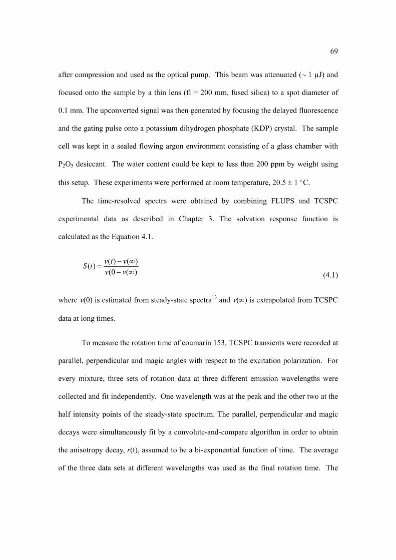
69
after compression and used as the optical pump. This beam was attenuated (~ 1 µJ) and
focused onto the sample by a thin lens (fl = 200 mm, fused silica) to a spot diameter of
0.1 mm. The upconverted signal was then generated by focusing the delayed fluorescence
and the gating pulse onto a potassium dihydrogen phosphate (KDP) crystal. The sample
cell was kept in a sealed flowing argon environment consisting of a glass chamber with
P2O5 desiccant. The water content could be kept to less than 200 ppm by weight using
this setup. These experiments were performed at room temperature, 20.5 1 C.
The time-resolved spectra were obtained by combining FLUPS and TCSPC
experimental data as described in Chapter 3. The solvation response function is
calculated as the Equation 4.1.
)(0(
)()()(
vv
vtvtS
(4.1)
where (0) is estimated from steady-state spectra13 and () is extrapolated from TCSPC
data at long times.
To measure the rotation time of coumarin 153, TCSPC transients were recorded at
parallel, perpendicular and magic angles with respect to the excitation polarization. For
every mixture, three sets of rotation data at three different emission wavelengths were
collected and fit independently. One wavelength was at the peak and the other two at the
half intensity points of the steady-state spectrum. The parallel, perpendicular and magic
decays were simultaneously fit by a convolute-and-compare algorithm in order to obtain
the anisotropy decay, r(t), assumed to be a bi-exponential function of time. The average
of the three data sets at different wavelengths was used as the final rotation time. The
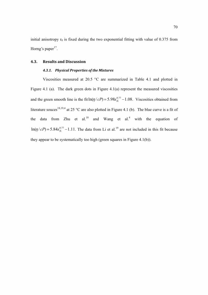
70
initial anisotropy r0 is fixed during the two exponential fitting with value of 0.375 from
Horng’s paper17.
4.3. Results and Discussion
4.3.1. Physical Properties of the Mixtures
Viscosities measured at 20.5 C are summarized in Table 4.1 and plotted in
Figure 4.1 (a). The dark green dots in Figure 4.1(a) represent the measured viscosities
and the green smooth line is the fit 1.085.98)/ln( 0.77 ILxcP . Viscosities obtained from
literature souces18,19,4 at 25 °C are also plotted in Figure 4.1 (b). The blue curve is a fit of
the data from Zhu et al.18 and Wang et al.4 with the equation of
1.115.84)/ln( 0.77 ILxcP . The data from Li et al.19 are not included in this fit because
they appear to be systematically too high (green squares in Figure 4.1(b)).

71
xIL
0.0 0.2 0.4 0.6 0.8 1.0
/ c
P
1
10
100
xIL
0.0 0.2 0.4 0.6 0.8 1.0
/ c
P
0.1
1
10
100
20.5 oC
Literature
25 oC
(b)
(a)
Figure 4.1: Measured and literature viscosity values of the mixtures. (a) The measured
viscosities at 20.5 C (symbols) plotted vs. the ionic liquid mole fraction. The dark green curve is
the fit of these data (see text). The dashed blue curve reproduces the fit to the 25 C data in panel (b) for comparison.
(b). Literature viscosity data at 25 C. Black circles, red triangles and green squares represent data from Zhu et al.18, Wang et al.4 and Li et al.19, respectively. The blue curve is a fit of the data of Zhu et al. 18 and Wang et al.4

72
Table 4.1: Mixtures studied and some of their properties.
xIL IL g ml nD f(nD2) /cP
D(ACN)/
10‐11m2s‐1
D(Im41+)/
10‐11m2s‐1
0.00 0.000 0.788 1.3414 0.210 0.35 485
0.10 0.285 0.911 1.3705 0.226 0.87
0.20 0.473 0.990 1.3879 0.236 1.84 144.2 50.6
0.30 0.606 1.046 1.3975 0.241 3.72
0.40 0.705 1.086 1.4037 0.244 6.58 58.9 20.2
0.50 0.782 1.117 1.4088 0.247 11.85
0.60 0.843 1.140 1.4125 0.249 18.78 23.4 6.4
0.80 0.935 1.173 1.4182 0.252 53.27 12.1 2.9
0.90 0.970 1.185 1.4202 0.253 84.17 8.3 2
1.00 1.000 1.194 1.4212 0.254 130.13 1.6
Note: All data are at 25 C except for viscosities which were measured at 20.5 C. The uncertainty of the refractive index (nD) is 0.0004 and the viscosity () data has 1% uncertainty. xIL represents the mole fraction and IL is the volume fraction. D(ACN) and D(Im41
+) represent
the diffusion coefficient of acetonitrile and cation of the ionic liquids, respectively. * The
density data is from literature Huo et al 2007.11
Refractive indices (nD, Table 4.1) were measured for use in considering the
solvatochromism of C153 in the following section. Most relevant to this use is the
reaction field factor )( 2Dnf , plotted in Figure 4.2.
2
1)(
2
22
D
DD n
nnf (4.2)
These data are conveniently fit to a function .)( 232 dcbanf ILILILD where IL
is the volume fraction of the ionic liquid, a=0.0057, b=-0.0271, c=0.0649 and d=0.2103.

73
The green line is the function )()1()()( 2,
2,
2ACNDILILDILD nfnfnf , expected for
“ideal” mixtures.
xIL 0.0 0.2 0.4 0.6 0.8 1.0
0.0 0.2 0.4 0.6 0.8 1.0
f(n D
2 )
0.20
0.21
0.22
0.23
0.24
0.25
0.26
IL
Figure 4.2: Plots of reaction field factor )( 2Dnf vs. the mole fraction xIL (black circles) and the
volume fraction IL (blue squares). The blue curve is the fitting
.)( 232 dcbanf ILILILD (see text). The green line is linear behavior of a ideal
mixture.20
As mentioned in the Experimental section, the self-diffusion coefficients of the
cation and acetonitrile components at some mixture compositions were obtained from
NMR measurement. The results are provided in Table 4.1. There are some simulation
data for this mixture from Chaban and Prezhdo3 who simulated the diffusion rates using a
new force field model. Figure 4.3 shows the plots of the diffusion rates of cation Im41+
and the acetonitrile versus the [Im41][BF4] mole fraction. The black circles represent the

74
simulation data from Chaban and Prezhdo3 and the red triangles are the NMR results.
The red lines are the fitting functions from the experimental data,
)8.4exp(4.131)(Im41 ILxD and )1.4exp(6.293)8.12exp(4.191)( ILIL xxACND .
There is reasonable agreement between the simulated and measured diffusion rates.
(a)
xIL
0.0 0.2 0.4 0.6 0.8 1.0
D/ 1
0-11 m
2 s-1
1
10
100
Chaban 2011 This work
(b)
xIL
0.0 0.2 0.4 0.6 0.8 1.0
D/ 1
0-11 m
2 s-1
10
100
1000
Chaban 2011 This work
Figure 4.3: Measured and simulated diffusion coefficients of the mixtures. (a) Diffusion rates of the cation [Im41+] from simulation data of Chaban and Prezhdo3 (black circle), the NMR measurement (red triangle) and the fitting for experimental results (red line, see text). (b) diffusion rates of acetonitrile.

75
The diffusion coefficients (DSE) are also calculated from Stokes-Einstein equation
with stick boundary condition.
i
Bi R
TkD
6
(4.3)
Where kB represents Plank’s constant, viscosity and R the diffusor’s radius. The van der
Waals volumes of Im41+, BF4
- and acetonitrile are 163.5, 50.5 and 47.1 Å3 respectively.
The calculated radii are 3.4 Å (Im41+), 2.3 Å (BF4
-) and 2.2 Å (ACN). The molecular
volume ratio Vu/Vv is the molecular volume of the diffusion target molecule over the
mixture solvent molecular volume which is the weighted volume of all three species.
Figure 4.4 (a) is the plot of the measured diffusion coefficients versus the reciprocal of
the solvent viscosities. The ratios of predicted and measured diffusion rate are plotted vs.
the molecular volume ratio Vu/Vv in Figure 4.4 (b). The dark green curve is the fitting
function from the literature values of measured ionic liquid diffusion coefficents.21 The
ratios are correlated to Vu/Vv in roughly the same manner as are solutes in neat ILs. The
weak conclusion is that there is not anything obviously unusual about the diffusion
coefficients in these mixtures.

76
1/ (1/cP)0.01 0.1 1 10
D/m
2 s-1
1e-11
1e-10
1e-9
1e-8
ACNIm41BF4
(a)
Vu/Vv1.0
DSE
/Dob
s
0.1
1
ACNIm41BF4
(b)
Figure 4.4: Observed and Stokes‐Einstein predicted diffusion coefficients. (a): correlation between the measured diffusion rates and the reciprocal of the viscosity. The fitting functions
are 19.92-)/1ln(77.0)ln( ACND and 20.90-)/1ln(86.0)ln( 441Im BFD .
(b): Ratios of the Stokes‐Einstein predicted and observed diffusion coefficients vs. the molecular
volume ratio Vu/Vv. The dark green curve is the correlating equation
1
1
p
v
u
obs
SE
V
Va
D
D
with a=1.96 and p=2.15, which was obtained from fitting literature ILs data.21

77
4.3.2. C153 Spectra and Energies
Normalized absorption and steady-state emission spectra of C153 in acetonitrile
(red dashed curves) and [Im41][BF4] (blue curves) are shown in Figure 4.5. For
comparison we also include spectra of the ionic liquid [Im41][BF4] plotted relative to the
C153/[Im41][BF4] spectra. The absorption and emission spectra of C153 in the two neat
solvents are similar and differ primarily in a small shift. The fluorescence of unavoidable
impurities in the [Im41][BF4] was not a concern relative to the much stronger emission
from the solute C153.
Wavelength / nm300 400 500 600 700
Rel
ativ
e In
tens
ity
0.0
0.2
0.4
0.6
0.8
1.0
Figure 4.5: Steady state absorption and emission spectra of C153 in pure acetonitrile (red, short dash) and in pure [Im41][BF4]
(blue, solid). Spectra of pure [Im41][BF4] (dark green, dash‐dot),
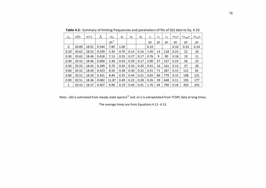
78
Table 4.2: Summary of limiting frequencies and parameters of fits of S(t) data to Eq. 4.10.
xIL v(0) v() fG G a1 a2 a3 1 2 3 <G> <exp> <sol>
ps‐1 ps ps ps ps ps ps
0 20.89 18.91 0.544 7.85 1.00 0.33 0.16 0.33 0.24
0.20 20.62 18.52 0.539 5.39 0.70 0.14 0.16 1.40 14 118 0.23 22 10
0.30 20.62 18.46 0.418 7.13 0.55 0.27 0.17 0.76 9 90 0.18 19 11
0.40 20.55 18.46 0.600 5.38 0.43 0.39 0.17 2.00 37 237 0.23 56 23
0.50 20.55 18.45 0.189 9.70 0.56 0.24 0.20 0.41 16 161 0.13 37 30
0.60 20.52 18.40 0.423 8.50 0.38 0.30 0.32 0.55 71 287 0.15 112 65
0.80 20.51 18.39 0.341 8.40 0.35 0.44 0.21 0.65 86 779 0.15 198 131
0.90 20.51 18.36 0.082 11.87 0.49 0.23 0.28 0.26 39 648 0.11 193 177
1 20.53 18.37 0.307 6.98 0.19 0.40 0.41 1.76 64 790 0.18 350 243
Note: (0) is estimated from steady‐state spectra13 and () is extrapolated from TCSPC data at long times.
The average times are from Equations 4.11‐ 4.13.

79
Frequency data are summarized in Table 4.2. The emission peak frequencies of
C153 in the mixtures at time-zero are estimates as described in Section 2.2.3.
Frequencies at time infinity are from the deconvoluted TCSPC data. The fitting
parameters of solvation response function and the solvation correlation time are also
provided in Table 4.2.
xIL
0.0 0.2 0.4 0.6 0.8 1.0
23.4
23.6
23.8
24.0
xIL
0.0 0.2 0.4 0.6 0.8 1.0
18.4
18.6
18.8
19.0
Pea
k F
requ
ency
vpk
/ 10
3 cm
-1
Absorption
Emission
(a)
(b)
xIL
23.4
23.6
23.8
24.0
f(nD2)
0.20 0.21 0.22 0.23 0.24 0.25 0.26
18.4
18.6
18.8
19.0
Absorption
Emission
(c)
(d)
Figure 4.6: Peak frequencies of the absorption and emission spectra. (a). The steady‐state
absorption peak frequency vs. mole fraction of the ionic liquid; (b). The emission peak
frequency (open circle) and emission peak frequency at time infinity (filled circle) vs. mole
fraction of the ionic liquid.
(c) & (d). Peak frequencies vs. reaction field factor f(nD2).
In Figure 4.6, the peak frequencies of the emission and absorption spectra are
plotted versus mole fraction of the ionic liquid (a, b) and the reaction field factor
2
1)(
2
22
D
DD n
nnf (c, d). The peak frequencies at time infinity are also plotted in figure 4

80
to compare to the steady state frequency shift. The time infinity spectra are obtained
from TCSPC setup using 20 ns time window. The frequency trend is similar to the one
from steady state results. The peak frequencies of steady-state and at infinity time are
nearly equal when sol <fluor (here in the mixtures with xIL closes to 0.). One could
interpret the nonlinearity versus xIL as being a result of preferential solvation but the
)( 2Dnf results say otherwise. Figure 4.6 (c) and (d) indicate that the peak frequencies are
approximately linearly related to the reaction field factor very well, which means that
there is no preferential solvation.
The solvation free energy difference ( Gsol ) of C153 between the ground state
and the excited state, and the reorganization energy sol were also calculated based on
the following equations: 22
0)]([2
1GvvhG abssol (4.4)
)]()0([2
1 vvhsol (4.5)
where vabs is the peak frequency of the absorption spectrum, h is the Planck’s constant,
∆G0 is the gas phase value estimated from a dielectric extrapolation in conventional
solvents. Here 295.9 kJ/mol is used as the value of ∆G0 which is taken from the
literature.22

81
f(nD2)
0.20 0.21 0.22 0.23 0.24 0.25 0.26
G /
kJ m
ol-1
-46
-44
-42
-40
-38
xIL
0.0 0.2 0.4 0.6 0.8 1.0
/ k
J m
ol-1
11.0
11.5
12.0
12.5
13.0
13.5
14.0
(b)
(a)
Figure 4.7: The solvation free energy and reorganization energy. (a). The correlation between
the solvation free energies and the reaction field factor f(nD2). )(45.12910.13 DnfG
(b).The reorganization energies are fitted to a function corresponding to the mole fraction of
ionic liquid. )}47.14exp(1{93.027.12 ILx
The solvation energy is calculated from Equation 4.4 and plotted in Figure 4.7
(a). The reorganization energy is also plotted in Figure 4.7 (b). The solvation free
energies and reorganization energies are plotted versus the reaction field factor and the
mole fraction of the ionic liquid, respectively. The solvation free energies is close to a

82
linear function of )( 2Dnf suggesting that the main source of the variation with
composition is the difference in electronic polarizabilities of acetonitrile and
[Im41][BF4]. The reorganization energies are fit to a smooth curve to see the trend. Our
original assumption was that one would expect to see a constant value of sol due to the
similar polarity of acetonitrile and [Im41][BF4], but the data shows a different story.
Obviously, the reorganization energy of pure acetonitrile is lower than the mixtures and
pure ionic liquid by 7%.
4.3.3. C153 Rotational Dynamics
Fluorescence anisotropy data were fit to the function
)]exp()exp([)(2
21
10 t
at
artr (4.6)
Fit parameters are summarized in Table 4.2. In these fits the initial anisotropy r0 is
fixed at the value of 0.375, derived from the frozen-solvent data reported in Ref.17 The
rotational correlation time is then obtained by the following equation,
2211 aarot (4.7)
Table 4.3: Parameters of Biexponential Fits to Fluorescence Anisotropy Data
xIL 0.2 0.3 0.4 0.5 0.6 0.8 0.9 1
a1 0.30 0.31 0.31 0.43 0.24 0.20 0.18 0.21
1 / ps 13 49 72 200 118 172 154 67
a2 0.70 0.69 0.69 0.57 0.76 0.80 0.82 0.79
2 / ns 0.15 0.27 0.41 0.94 1.23 2.71 3.74 5.24
<rot>/ns 0.11 0.20 0.31 0.62 0.97 2.21 3.10 4.18
Unc */ns 0.01 0.02 0.07 0.09 0.10 0.17 0.19 0.45Note: * The uncertainty is obtained from the 95% confidence limit for three measurements.

83
Figure 4.8 shows the correlation between rotation time and viscosity. The line
shows the fit )/ln(9.01.4ln cProt . The relation 0.9 is close to
hydrodynamic expectations.17 The inset in Figure 4.8 is the rotational coupling constant
(Crot) versus xIL where Crot is given by
stick
obs
stick
obsrotC
(4.8)
The hydrodynamic prediction using stick boundary condition is
TkLL
Vf
B
Lstick )1(
6)(
(4.9)
where L is the rank of the orientational correlation function (L=2 here),17 V the
molecular volume (246 Å3), and f the shape factor (1.71).17 From the results of Horng
et al.17, for dipolar solvents, 09.057.0 rotC . In these mixtures we find that Crot
decreases from 0.6 to 0.3 with the increase of mole fraction of the ionic liquid (inset of
Figure 4.8). The observed rotation time is faster with the increase of mole fraction of
[Im41][BF4] compared to the stick hydrodynamic prediction, which may be caused by
the preferential solvation of C153. Horng et al17 point out that the rotation time of C153
depends on solvent size from a molecular perspective. The solvent size increases with
the increase of the ionic liquid mole fraction. The rotational coupling constant is
decreasing with xIL increasing.
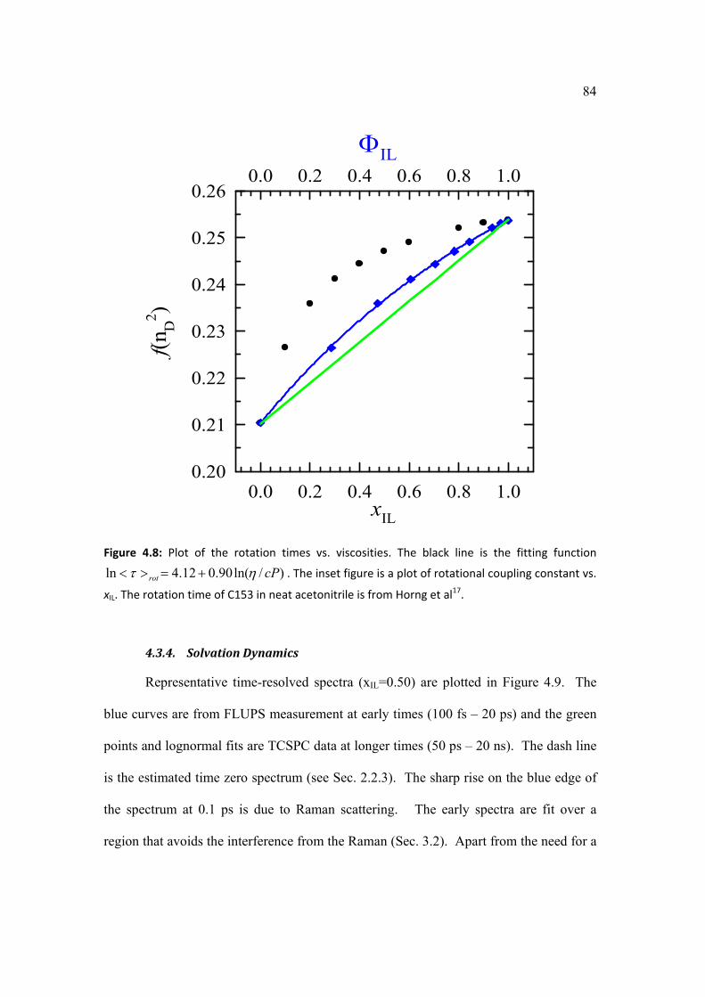
84
xIL 0.0 0.2 0.4 0.6 0.8 1.0
0.0 0.2 0.4 0.6 0.8 1.0f(
n D2 )
0.20
0.21
0.22
0.23
0.24
0.25
0.26
IL
Figure 4.8: Plot of the rotation times vs. viscosities. The black line is the fitting function
)/ln(90.012.4ln cProt . The inset figure is a plot of rotational coupling constant vs.
xIL. The rotation time of C153 in neat acetonitrile is from Horng et al17.
4.3.4. Solvation Dynamics
Representative time-resolved spectra (xIL=0.50) are plotted in Figure 4.9. The
blue curves are from FLUPS measurement at early times (100 fs – 20 ps) and the green
points and lognormal fits are TCSPC data at longer times (50 ps – 20 ns). The dash line
is the estimated time zero spectrum (see Sec. 2.2.3). The sharp rise on the blue edge of
the spectrum at 0.1 ps is due to Raman scattering. The early spectra are fit over a
region that avoids the interference from the Raman (Sec. 3.2). Apart from the need for a

85
small frequency correction of the FLUPS data, we generally find good agreement
between the spectra obtained using the two techniques. The spectra narrow somewhat in
time but the primary feature of these spectra is a frequency shift of ~200 cm-1.
Frequency / 103 cm-116 18 20 22 24
Rel
ativ
e In
tens
ity
0.0
0.2
0.4
0.6
0.8
1.0
0.1 ps
20 ns
Figure 4.9: Representative time‐resolved spectra of C153 in the XIL= 0.5 mixture. The blue curves are from FLUPS measurement at times of 0.1, 0.3, 0.5, 1, 2, 5, 10 and 20 ps. Green points are TCSPC data at times of 0.05, 0.1, 0.2, 1, 5 and 20 ns and the smooth green curves are lognormal fits to these data. The black dashed curve shows the estimated time‐zero spectrum.
Peak frequency data from the FLUPS and TCSPC experiments were combined
as described in Sec. 3.2 and used to calculate the spectral response function
.)()0(
)()()(
vv
vtvtSv To summarize the Sv(t) data they were fit to a function consisting
of one Gaussian and three exponential components,

86
)]exp()1()exp()exp([
)1(])(2
1exp[)(
321
22
11
2
taa
ta
ta
ftftS GGG
(4.10)
The Gaussian function represents the fast inertial component of the response and the
remainder represents the slower diffusive components. The integral time of the
Gaussian portion is given by
0
12/122
2533.1
2)
2exp(
GG
GG dt
t
(4.11)
and that of the remainder by
3212211exp )1( aaaa (4.12)
The total solvation time is then calculated as
exp)1( GGGsol ff (4.13)
The fit parameters and solvation time of all mixtures are tabulated in Table 4.2.
Figure 4.10 shows the quality of the fits of some representative response functions.
Figure 4.10(a) shows the solvation response of mixtures with the ionic liquid mole
fraction of 0.3, 0.5 and 0.8. Figure 4.10 (b) represents the spectral response from
experimental results of all mixtures.

87
Time / ps10-1 100 101 102 103
Sol
vati
on R
espo
nse
S(t)
0.0
0.2
0.4
0.6
0.8
1.0 (a)
Time / ps
10-1 100 101 102 103
Spe
ctra
l Res
pons
e S(
t)
0.0
0.2
0.4
0.6
0.8
1.0xIL=0
xIL=0.2
xIL=0.3
xIL=0.4
xIL=0.5
xIL=0.6
xIL=0.8
xIL=0.9
xIL=1
(b)
Figure 4.10: Observed solvation response functions. (a). Three solvation response functions (dots) and fits to Eq. 4.10 (solid line): xIL=0.3 (blue), xIL=0.5 (red) and xIL=0.8 (green). (b). S(t) summary plot of experimental data.
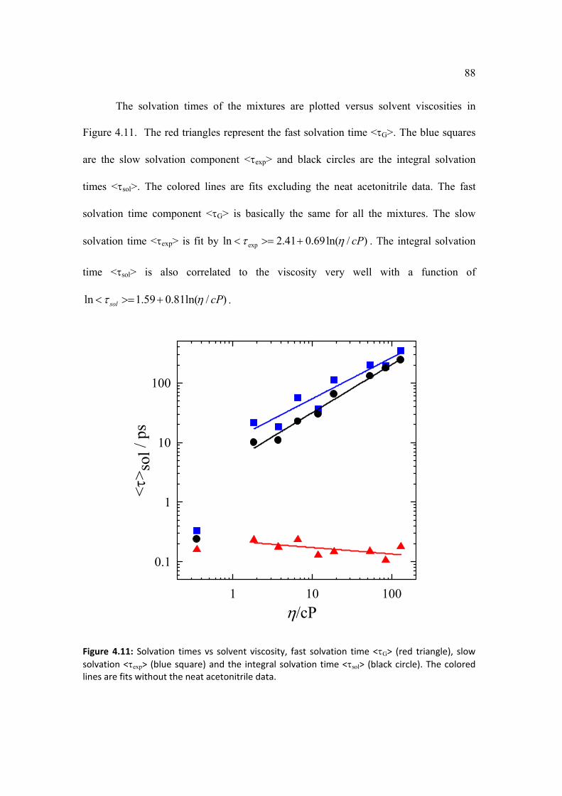
88
The solvation times of the mixtures are plotted versus solvent viscosities in
Figure 4.11. The red triangles represent the fast solvation time <G>. The blue squares
are the slow solvation component <exp> and black circles are the integral solvation
times <sol>. The colored lines are fits excluding the neat acetonitrile data. The fast
solvation time component <G> is basically the same for all the mixtures. The slow
solvation time <exp> is fit by )/ln(69.041.2ln exp cP . The integral solvation
time <sol> is also correlated to the viscosity very well with a function of
)/ln(81.059.1ln cPsol .
/cP1 10 100
<>
sol /
ps
0.1
1
10
100
Figure 4.11: Solvation times vs solvent viscosity, fast solvation time <G> (red triangle), slow
solvation <exp> (blue square) and the integral solvation time <sol> (black circle). The colored lines are fits without the neat acetonitrile data.
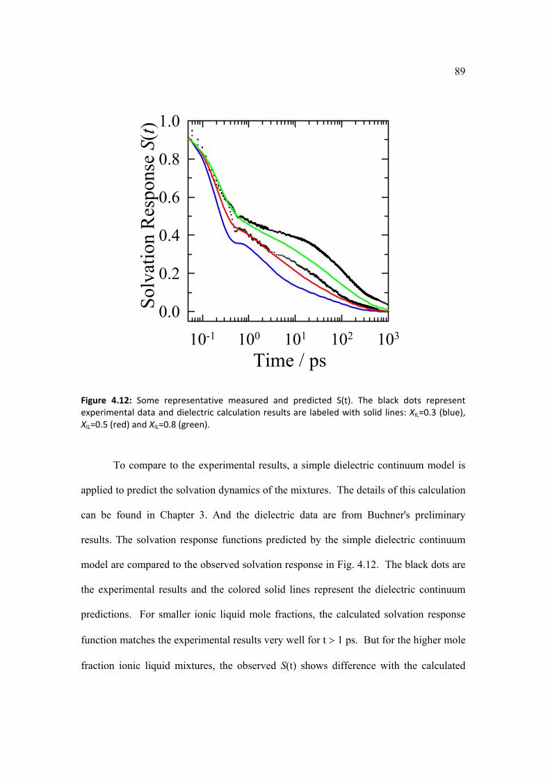
89
Time / ps10-1 100 101 102 103
Sol
vati
on R
espo
nse
S(t)
0.0
0.2
0.4
0.6
0.8
1.0
Figure 4.12: Some representative measured and predicted S(t). The black dots represent experimental data and dielectric calculation results are labeled with solid lines: XIL=0.3 (blue), XIL=0.5 (red) and XIL=0.8 (green).
To compare to the experimental results, a simple dielectric continuum model is
applied to predict the solvation dynamics of the mixtures. The details of this calculation
can be found in Chapter 3. And the dielectric data are from Buchner's preliminary
results. The solvation response functions predicted by the simple dielectric continuum
model are compared to the observed solvation response in Fig. 4.12. The black dots are
the experimental results and the colored solid lines represent the dielectric continuum
predictions. For smaller ionic liquid mole fractions, the calculated solvation response
function matches the experimental results very well for t 1 ps. But for the higher mole
fraction ionic liquid mixtures, the observed S(t) shows difference with the calculated

90
data at time range from 1 ps to 1 ns. As we know, the dielectric continuum model
predicts the solvation response very well for conventional solvents but not very well for
ionic liquids (Chapter 3). This may be the reason that we see bigger deviation for higher
mole fraction of the ionic liquid.
Dielectric calculated time / ps10-2 10-1 100 101 102 103
Mea
sure
d ti
me
/ ps
0.01
0.1
1
10
100
1000
S(t)=0.1S(t)=0.3 S(t)=0.5S(t)=0.7
S(t)
0.1
0.3
0.5
0.7
Figure 4.13: Comparison of the solvation response times of measured and predicted response functions at certain S(t) values, 0.1(black), 0.3(red), 0.5(green) and 0.7(blue). The inset plot shows the meaning of these times.
As a means of assessing the level of agreement between the observed and
calculated response functions we compare the times required for S(t) to reach values of
0.1, 0.3, 0.5 and 0.7. This comparison is provided in Figure 4.13. For example, for the
0.5 ionic liquid mole fraction mixture, the observed time for S(t) reaches 0.3 is 4.1 ps

91
and the predicted time at 0.3 of S(t) is 3.3 ps. The point plotted in Figure 13 is then
(3.33, 4.12). The outstanding green square is the S(t)=0.5 point of C153 in the pure
ionic liquid. Except for this point, the observed solvation times are highly correlated to
the predicted times, even though the measured and calculated solvation dynamics differ
systematically at long times.
4.4. Summary and Conclusions
Solvation dynamics of the acetontrile and 1-butyl-3-methylimidazolium
tetrafluoroborate were measured using the standard probe coumarin 153. Combing the
FLUPS technique which has 80 fs time resolution with TCSPC, the entire solvation
response is captured. The validity of the simple dielectric continuum model is tested
against these mixture data. The measured solvation response functions are matched well
with the calculated results. The rotation times of C153 in all the mixtures are measured
and correlated well to the viscosity. The diffusion coefficient measured NMR
experiments are matched well with the simulated diffusion coefficients.

92
Notes and References
(1) Daschakraborty, S.; Ranjit, B. J. Phys. Chem. B 2011, 115, 4011.
(2) Mellein, B. R.; Aki, S. N. V. K.; Ladewski, R. L.; Brennecke, J. F.
Journal of Physical Chemistry B 2007, 111, 131.
(3) Chaban, V. V.; Prezhdo, O. V. Phys. Chem. Chem. Phys. 2011, 13,
19345.
(4) Wang, J.; Tian, Y.; Zhao, Y.; Zhuo, K. Green Chemistry 2003, 5, 618.
(5) Zafarani-Moattar, M. T.; Shekaari, H. Journal of Chemical
Thermodynamics 2006, 38, 1377.
(6) Chakrabarty, D.; Chakraborty, A.; Seth, D.; Sarkar, N. Journal of
Physical Chemistry A 2005, 109, 1764.
(7) Mellein, B. R.; Aki, S. N. V. K.; Ladewski, R. L.; Brennecke, J. F.
Journal of Physical Chemistry B 2007, 111, 131.
(8) Jin, H.; Baker, G. A.; Arzhantsev, S.; Dong, J.; Maroncelli, M. Journal of
Physical Chemistry B 2007, 117, 7291.
(9) Gardecki, J. A.; Maroncelli, M. Applied Spectroscopy 1998, 52, 1179.
(10) Wu, D.; Chen, A.; Johnson, C. S., Jr. Journal of Magnetic Resonance,
Series A 1995, 115, 260.
(11) Huo, Y.; Xia, S.; Ma, P. Journal of Chemical & Engineering Data 2007,
52, 2077.
(12) H. Vogel, P. Z., 645, 1921; G. S. Fulcher, J. Am. Ceram. Soc. 8, 339,
1925; G. Tammann and W. Hesse, Z. Anorg. Allg. Chem. 156, 245, 1926.
(13) Fee, R. S.; Maroncelli, M. Chemical Physics 1994, 183, 235.
(14) Horng, M. L.; Gardecki, J.; Papazyan, A.; Maroncelli, M. J. Phys. Chem.
1995, 99, 17311.
(15) Zhang, X. X.; Wuerth, C.; Zhao, L.; Resch-Genger, U.; Ernsting, N. P.;
Sajadi, M. Rev. Sci. Instrum. 2011, 82, 063108/1.
(16) Zhao, L.; Luis Perez Lustres, J.; Farztdinov, V.; Ernsting, N. P. Physical
Chemistry Chemical Physics 2005, 7, 1716.
(17) Horng, M. L.; Gardecki, J. A.; Maroncelli, M. J. Phys. Chem. A 1997,
101, 1030.

93
(18) Zhu, A.; Wang, J.; Han, L.; Fan, M. Chem. Eng. J. (Amsterdam, Neth.)
2009, 147, 27.
(19) Li, W.; Zhang, Z.; Han, B.; Hu, S.; Xie, Y.; Yang, G. Journal of Physical
Chemistry B 2007, 111, 6452.
(20) Marcus, Y. Solvent Mixtures. Properties and Selective SolvationNew
York, 2002.
(21) Kaintz, A.; Benesi, A.; Baker, G.; Maroncelli, M. 2012, manuscript in
preparation.
(22) Jin, H.; Baker, G. A.; Arzhantsev, S.; Dong, J.; Maroncelli, M. J. Phys.
Chem. B 2007, 111, 7291.

94
Chapter 5. Experimental Bimolecular Electron Transfer Between the 9,10-dicyanoanthracene and N,N-dimethylaniline
in Ionic Liquids
2.
Reproduced in part with permission from
Min Liang, Anne Kaintz, Gary A. Baker, and Mark Maroncelli
J. Phys. Chem. B, 2012, 116 (4), pp 1370–1384
Other People’s contributions:
Anne Kaintz measured the diffusion coefficients. Gary Baker made all pyrrolidinium ionic
liquids.

95
5.1.Introduction
Among the myriad uses for which ionic liquids are currently being investigated,
numerous applications fall within the area of energy generation and storage.1 For
example, the low volatility, intrinsic conductivity, and tailorabiliy of ionic liquids afford
significant advantages over conventional organic solvents in devices such as fuel cells,
supercapacitors and batteries, and dye-sensitized solar cells.2,3 Electron transfer is a key
component of many such applications and for this reason it is important to achieve a
sound understanding of the nature of electron transfer processes in ionic liquids. In
particular, it is important to learn to what extent the theoretical approaches developed for
treating electron transfer in conventional solvents are also applicable to ionic liquids.
Toward this end many electrochemical studies of heterogeneous electron transfer have
been performed.4,5 These studies have shown that while the mechanisms of reaction are
typically the same as in high-polarity conventional solvents, the high viscosities of ionic
liquids often produce much slower rates. Some interesting attempts have been made to
relate heterogeneous reaction kinetics to fundamental theories of electron transfer,6 but
the largely unknown and apparently complex structure of ionic liquid – electrode
interfaces7 renders comparison to theory difficulty. In the case of homogeneous electron
transfer, simulations8-11 and recent experimental studies of photo-induced intramolecular
processes12 suggest that electron transfer is comparable in ionic liquids and high-polarity
conventional solvents. The primary difference found in ionic liquids is a marked
decrease in rates caused by the much slower and highly dispersed solvation dynamics
characteristic of these solvents.13,14

96
Table 5.1: Diffusion‐Limited Bimolecular Reactions in ILs
# Reaction(a) Ionic Liquids(b) /cP(c) [Q]/M(c) 0/ns(c) kq/kD(c) Technique(d) Ref.
1 C15n* + DMA C15n- + DMA+ [Im51][BF4] 135 .5-1.5 1-4 100-170 ps FL 23
2 C15n* + DMA C15n- + DMA+ [Im21][Tf2N] 31 .05-.25 1-3 5-8 ps FL 21
3 C15n* + DMA C15n- + DMA+ DAF 75 .01-.08 1-3 33-35
130-150 ps FL SS FL
20
4 BPH* + CCl4 BPH+ + CCl4- [Im41][Tf2N] 49 .01-.12 5 16 ns TA 22
5 DCA* + D DCA- + D+ [Imn1][PF6] n=4,8 350, 570 0.4-1.1 12, 13 85, 150 SS FL 19
6 Py* + DMA Py- + DMA+ 4 Im ILs 34-330 .01-.06 300 2-4 ns FL & TA 81
7 BuPy + DQ BuPy+ + DQ- 5 N &Pr ILs 80-700 < .004 ~5104 5-14 radiolysis 17
8 3Bp* + NaphBp + 3Naph* 5 Im ILs 50-700 < .003 >2000 3-12 ns TA 16
9 Ru(bpy)3
*2+ + MV2+Ru(bpy)33+ +
MV+ [Im41][PF6] 260 < .015 ~2000 1.1 ns TA 15
10 I2- + I2
- I3- + I- 6 assorted ILs 55-300 (<10-5) -- 1.0-1.8 ns TA 82
11 MV+ + MV2+ MV2+ + MV+ 3 Im ILs 10-12 (510-4) -- .32-.34 ESR lineshape 18
(a) C15n = various coumarin dyes (151, 152, …), DMA = N,N-dimethylaniline, BPH = ketyl radical, DCA = 9,10-dicyanoanthracene, D = various amine donors, Py = pyrene, MV = methylviologen, BuPy = n-butylpyridine, DQ = duraquinone, Bp = benzophenone, Naph = naphthalene, Ru(bpy)3 = ruthenium tris-bipyridine (b) Imn1 designates a methylimidazolium cation with a CnH2n+1 substituent, DAF = N,N-dimethylethlyammoniumformate, and Im, N, and Pr respectively denote imidazolium, ammonium, and pyrrolidinium ionic liquids.
(c) denotes solvent viscosity, [Q] the “quencher” (abundant reactant) concentration, 0 the “fluorophore” (rare reactant) lifetime in the absence of
quencher, kqthe observed bimolecular rate constant, and kD the rate constant calculated from 3/8 Tkk BD .
(d) FL = fluorescence, SS = steady state, TA = transient absorption

97
Bimolecular electron transfer reactions, the subject of the present work, have been
previously studied by several groups.15-23 In a number of cases, the rates of reactions
known to be diffusion limited in conventional solvents show what on first glance appear
to be anomalously high rates in ionic liquids. Table 5.1 documents some of the results
currently available. In one of the earliest studies (#8 in Table 5.1) McLean et al.
measured the electron transfer quenching of triplet benzophenone in five ionic liquids and
two conventional solvents as a function of temperature.16 Whereas the rates observed in
the solvents acetonitrile and toluene were close to expectations for a diffusion-limited
process, 3/8 Tkk BD , McLean et al. noted that the rates in ionic liquids were up to an
order of magnitude larger. (kB is Boltzmann’s constant, T the temperature, and the
solution viscosity.) Similar observations were made in another early study by
Skrzypczak and Neta17 (#7) who measured rates of electron transfer between the
butylpyridinyl radical and duraquinoneto be 5-14 times larger than expected based on
viscosity-scaling rates observed in conventional solvents. Skrzypczak and Neta proposed
that these high rates were the result of reactants diffusing more rapidly than would be
expected based on the high bulk viscosities of ionic liquids. But enhanced diffusion is
unlikely to account for some of the very high values of kq/kD shown in Table 5.1. For
example, using a Stern-Volmer analysis of steady-state fluorescence data on the electron
transfer quenching of S1 9,10-dicyanoanthracene by amine donors, Viera and Falvey
reported values of kq/kD> 50 in two high-viscosity ionic liquids.19 Similarly high values
were reported in independent studies of the fluorescence quenching of excited coumarin
dyes by the groups of Sarkar(#3) and Bhattacharyya (#1). But there are also several cases
(#2 and #6) in which neutral solutes show only modest rate enhancements compared to

98
expectations. In addition, in one study (#3), Stern-Volmer analysis of steady-state and
time-resolved fluorescence data produced very different bimolecular rate constants. To
date, no explanation for these varied results has been offered, and it is far from clear what
it is about the ionic liquid environment that sometimes produces unexpectedly high
bimolecular electron transfer rates.
In the present study we take a closer look at these issues and attempt to explain
some of the apparently anomalous behavior observed. We report steady-state and time-
resolved emission measurements of the electron transfer quenching of S1 9,10-
dicyanonanthracene (DCA) by N,N-dimethylaniline (DMA) in ionic liquids and
conventional solvents. The DCA + DMA system was chosen in part because of the
extreme values of (kq/kD) reported by Viera and Falvey19 for strong electron donors like
DMA. The long lifetime (~13 ns) of DCA and the fact that this solute shows only a very
small dynamic Stokes shift also prove useful in the present work. The sort of data we
collect in ionic liquids is qualitatively similar to what has been reported in previous
studies. One distinction from prior work is that in addition to measuring the reaction in
low viscosity conventional solvents, we also make measurements in mixtures of ethylene
glycol + glycerol, which have viscosities (and polarities) comparable to those of ionic
liquids. These data show that the “anomalies” reported in ionic liquid solvents are in
large part due to their high viscosities and are not a special aspect of electron transfer in
ionic media. We also for the first time measure diffusion rates of one of the species
involved in the reaction (DMA) using NMR techniques. These measurements (and more
extensive work on other solutes24) show that diffusion of neutral solutes of moderate size

99
in ionic liquids is typically faster than hydrodynamic predictions, but usually only by
factors of 3-5.
The main way in which the present work differs from other ionic liquid studies to
date is that we attempt a much more detailed analysis of the bimolecular electron transfer
reaction. Instead of simply applying Stern-Volmer analyses25 to determine quenching
rate constants for comparison to the “diffusion limit” kD, we fit time-resolved emission
decays to a complete model which couples a classical Marcus description of the distance
dependent electron transfer process26 to a Smoluchoski-type spherical diffusion +
reaction approach27,28 to model the overall population kinetics. This sort of modeling has
been applied previously by the groups of Tachiya,29-32 Fayer,33-35 and most recently
Grampp36-38 to understand bimolecular electron transfer in conventional solvents. Rather
than solving the reaction-diffusion equations numerically as done by these other groups,
we employ the convenient analytical approximations derived recently by Dudko and
Szabo.39 To our knowledge this is the first time that this method has been employed to
model experimental data. We find that it is possible to satisfactorily model all of the
experimental quenching collected in high polarity conventional solvents and ionic liquids
using a single set of physically sensible parameters. This modeling makes it clear that
theories developed to treat electron transfer and diffusion-limited reaction in conventional
solvents apply equally well in ionic liquids. Once the much higher viscosities and the
poorer approximation provided by hydrodynamic predictions for diffusion are accounted
for, the rates of bimolecular electron transfer reactions in ionic liquids do not appear
anomalous or distinctive.

100
5.2.Experimental Methods
9,10-dicyanoanthracene (DCA) was obtained from TCI-America (97%) and was
recrystallized from a mixture of pyridine + acetonitrile prior to use. N,N-dimethylaniline
(DMA; 99.5+%), cyclohexane and acetonitrile (HPLC grade), ethylene glycol (99.8%),
and glycerol (99.5%) were obtained from Sigma-Aldrich and were used as received. The
series of N-alkyl-N-methylpyrrolidiniumbis(trifluoromethylsulfonyl)imides, [Prn1][Tf2N]
with n = 3, 4, 6, 8, 10, were prepared as described in Ref.40
Propyltrimethylammoniumbis(trifluoromethylsulfonyl)imide, [N3111][T2fN], was
obtained from Kanto Chemical and 1-butyl-3-methylimidazolium hexafluorophostphate,
[Im41][PF6], from Iolitec (99%) and were used as received except for drying.
Decyltrimethylammoniumbis(perfluoroethanesulfonyl)imide, [N10,111][Beti], was
obtained by metathesis of the bromide salt (TCI America 99+%) and [Li][Beti].41 Finally,
tributyltetradecylphosphoniumbis(trifluoromethylsulfonyl)imide ([P14,666][Tf2N]) was
prepared as described in Ref.12 All of the ionic liquids were dried under vacuum at 45 °C
overnight prior to measurement. The water contents were measured using a Mettler-
Toledo DL39 Karl Fischer coulometer and were below 100 ppm by weight. Mixtures of
ethylene glycol + glycerol were made by weight and had water contents of <250 ppm.
Samples for optical spectroscopy were prepared in a nitrogen-purged glove box
using a stock solution of the fluorophore DCA in cyclohexane. The cyclohexane was
removed by evacuation prior to adding solvent. The optical densities of these samples
were maintained near 0.1 in 1 cm quartz cuvettes. Aliquots of the quencher DMA were
added directly to the cuvette samples using a micropipette. Estimated uncertainties in the

101
DMA concentration are between 16-6% over the range 0.05-0.3 M. All optical
measurements were maintained at constant temperature, usually 298 K.
Steady-state absorption spectra were measured using a Hitachi U-3000 UV/Vis
spectrometer at 1 nm resolution and steady-state fluorescence spectra recorded with a
SPEX Fluorolog 212 spectrometer (2 nm). The emission spectra were corrected for
detector sensitivity using a method based on a series of dye standards.42 Time-resolved
fluorescence data were recorded using a home-built time-correlated single photon
counting (TCSPC) setup.43 The excitation source (420 nm) was the doubled output of a
cavity-dumped Ti:sapphire laser (Coherent Mira 900F + APE PulseSwitch) operating at a
repetition rate of 3MHz. Fluorescence was collected at magic angle with respect to the
excitation polarization through a monochromator (ISA H10) with an emission bandpass
of 4 nm. The instrumental response of this setup was 25-30 ps (FWHM) as judged by the
signal from a scattering solution. Fluorescence decays having greater than 5000 peak
counts were collected over time windows of between 8-45 ns (4096 channels) depending
on sample lifetime. Decays were fit to multi-exponential functions using a convolute-
and-compare algorithm. Three decays were typically measured for each sample and an
averaged multi-exponential description used for analysis as described later.
The viscosities of the ionic liquid solutions and ethylene glycol + glycerol
mixtures were measured with a Brookfield Model HBDV-III+CP cone/plate viscometer.
The viscometer was calibrated using the NIST-certified viscosity standards N75 and
N100. In most cases, viscosities were measured from 5 to 65 °C with an increment of
5°C and fit to the Vogel-Fulcher-Tammann equation used to characterize these data.

102
Diffusion coefficients of DMA were determined from 1H data measured on
Bruker DRX-400 and AV-III-850 spectrometers using the longitudinal eddy current delay
stimulated echo pulse sequence with bipolargradient pulses.44 In the case of the
[Prn1][Tf2N] series of ionic liquids, diffusion measurements were made on DMA
solutions at a series of concentrations between 0 – 0.3 M and diffusion coefficients
extrapolated to infinite dilution. In this manner it was found that diffusion coefficients
measured with 50 mM DMA are within uncertainties (~8%) of the limiting values.
Diffusion coefficients of DMA in other solvents were therefore determined only at
[DMA] = 50 mM.
5.3. Modeling the Time-Dependent Quenching Process
5.3.1. The Formalism
Scheme 1
We assume quenching (Scheme 1) to be the result of irreversible electron transfer
between an excited fluorophore F* (DCA* here) and a quencher Q (DMA) as depicted in

103
Scheme 1. Measured fluorescence decays I(t) are assumed to be related to the time-
dependent reaction rate coefficient k(t) via
t
tdtkQtkF
tF
I
tI
0
0*
*
)(][exp)]0([
)]([
)0(
)( (5.1)
where [Q] indicates the concentration of quencher and k0 is the fluorescence decay rate
constant in the absence of quencher. k(t) is determined from the spherically symmetric
reaction – diffusion equation for the F* - Q pair distribution p(r,t):27,28,36
),()()](exp[)](exp[
1),( 22
trprrwr
rwrrr
Dt
trp
(5.2)
where D is the relative diffusion coefficient of F* and Q, assumed to be given by the sum
of the individual diffusion coefficients QFDDD * , w(r) is the potential of mean force
between F* and Q, 1)( TkB with kB being Boltzmann’s constant and T the
temperature, and (r) describes how the reaction rate varies with F* - Q separation r.
Finally, p(r,t) and k(t) are related by
drtrprtk ),(4)(0
2
(5.3)
Exact solution of Eq. 5.2 for k(t) is only possible in a few simple cases,45which do not
include situations in which (r) includes non-contact reactions appropriate to electron
transfer quenching. Before discussing solution of Eq. 5.2, we digress briefly to discuss
one case in which Eq. 5.2 is analytically solvable because the results are important for the
later discussion.
104
In the absence of significant F – Q interactions and when (r) is such that reaction
occurs instantaneously at some contact distance but not elsewhere, solution of Eq. 5.2
provides the prediction first obtained by Smoluchowski46
Dtktk D
2
1)( (5.4)
and
DttkQtkI
tID 2
0 8][exp)0(
)( (5.5)
with DkD 4 . If one can ignore the t or “transient term” in Eq. 5. 5, exponential
emission decays are predicted, and Stern-Volmer type of analysis25 of either steady-state
emission intensities or emission lifetimes as a function of quencher concentration yields
bimolecular rate constant equal to kD. For systems of the sort studied here, the value of
kD can be evaluated with moderate accuracy using the Stokes-Einstein predictions for
diffusion coefficients, RTkD B 6/ where is the solvent viscosity and R the radius
of the diffusing molecule. Denoting the radii of F* and Q by RF and RQ and assuming
QF RR , one obtains what we will refer to as the simple Smoluchowski prediction
for the diffusion-limited rate constant:47,48
QF
QFBD RR
RRTkk
4
)(
3
82
(5.6)
For comparably sized F and Q the term in parenthesis in Eq. 5. 6 is close to unity and one
has the remarkably simple prediction 3/8 Tkk BD used in Table 5.1. Like mentioned

105
in the experimental part, the viscosities were measured from 5 to 65 °C with an increment
of 5°C and fit to the Vogel-Fulcher-Tammann equation (5.7) and the fitted results were
applied to get kD valules.
KTT
BA
/)(cP)/ln(
0 (5.7)
Returning now to the more general case, to solve Eq. 5.2 for k(t) we rely on the
approximate solution proposed by Dudko and Szabo.39 These authors showed that k(t)
can be approximately expressed.
)]()(1)[()( 222
211
22
21 terfceterfcektk tt (5.8)
where the long-time limiting rate constant k()
)()( 111 DCkk (5.9)
is a composite of the reaction-limited rate constant <>, given by
0
)(2 )(4 drrer nrwn (5.10)
with n=1, and the long-time diffusion-controlled (“DC”) rate constant
0
2
0
)(22
)(
2
)(
4)(
drdxexxr
e
D
kr
xwrw
DC
(5.11)
The time-dependent portion of k(t) is written in terms of the parameters49

106
2
2
2,1 )(
and
1)(22,1
DCk (5.12)
where 2/3
2
8
)(
D
kDC
and
2
2
22 )]([
DCk (5.13)
Dudko and Szabo tested these expressions against numerical solutions of Eq. 5.2.45 In the
case of contact reactions (reaction only at r= as described above) they found this
approximation to be within a few percent of numerical solution of Eq. 5.2 for a wide
range of system parameters. In cases with significant distance dependence to reaction
they found more modest accuracies in the range 10-15%. Given that the distance
dependence of electron transfer can only be predicted semi-quantitatively, we view this
level of accuracy appropriate to our purposes.
To model the distance dependence of the quenching reaction we employ the semi-
classical form of the Marcus expression for non-adiabatic electron transfer:26,50,51
Tk
G
Tkh
V
BB
el
4
)(exp
4
1 22/12
(5.14)
where Vel is the electronic coupling, the reorganization energy, and G the driving
force for reaction. All three of these quantities are expected to depend upon the
separation between F* - Q, and we represent these dependences as follows. The
electronic coupling is expected to decrease exponentially with distance as
)}(exp{)( 02
02 rrVrV elel (5.15)
107
Where r0=RF+RQ and V0 is the electronic coupling at r0. The reorganization energy
consists of an intramolecular contribution and a solvent contribution
)()( rr solvra int . For the solvent contribution we use the 2-sphere dielectric
continuum expression of Marcus:52,53
rQF
solnrRR
er
111
2
1
2
1
)4()(
20
2
(5.16)
where 0 is the permittivity of free space, n the refractive index and r the relative
permittivity of the solvent. For the distance dependence of the driving force we adopt the
Rehm-Weller expression including the free energy of reactionG0 54
r
eGrG
r
1
)4()(
0
2
0 (5.17)
5.3.2. The Specification of Model Parameters
Application of the model just described requires specification of a number of
parameters characterizing the reactants, the electron transfer process, and the solvent.
For convenience these parameters are summarized in Table 5.2. How values of these
parameters were chosen is discussed below.

108
Table 5.2: Summary of Model Parameters used in Fitting Quenching Data
Parameter Value Use in Fits
RF – fluorophore radius 3.66 Å fixed
RQ – quencher radius 3.12 Å fixed
intra – intramolecular reorganization energy 0.4 eV fixed
V0 ‐ electronic coupling at r=RF+RQ 100 cm‐1 initially varied
el – coupling length scale parameter 1.5 Å‐1 fixed
r – relative permittivity 39 (or 2.0)a fixed
n – refractive index 1.42 fixed
G0 – free energy change ‐1.2 (or+0.8)aeV varied
0 – unquenched lifetime 10‐14 ns fixed at [Q]=0 value
FQ – size parameter of U(r) RF+RQ fixed
FQ – energy parameter of U(r) ~2.5 kJ/mol varied
Rh – effective hydrodynamic radius ~1.7 Å varied
(a) Values in parenthesis are used only in the case of cyclohexane solvent.
The fluorophore and quencher radii RF and RQ are determined assuming spherical
shapes and the van der Waals volumes55 of DCA and DMA. The intramolecular
reorganization energy is set at intra = 0.4 eV based upon values obtained from gas-phase
calculations at the B3LYP/6-31G(d) and MP2/6-31G(d,p) levels. The value of V0, the
electronic coupling at the “contact” distance RF+RQ, is a poorly defined quantity, as this
coupling is strongly dependent upon the relative orientations of the F-Q pair in addition
to the their separation,56-58 Computational studies56-58and analyses of experimental data
on similar systems29,36,37 suggest V0to be on the order of 100 cm-1 (12 meV). We
examined the effect that varying this parameter had on fits to the observed quenching
kinetics and ultimately fixed the value at 100 cm-1. Experimental and computational

109
work suggests that the decay constant el should lie within the range 1.0 el2.0Å-1 for
most solvents.56,59-61 We adopt a fixed value of el = 1.5 Å-1for all solvents studied here.
The reaction free energy can be estimated using the measured oxidation potential
E(Q/Q+) of the donor Q and the reduction potential E(F/F-) and 0-0 transition frequency
of the acceptor F(E00) via the relation:54
000 )/()/( EFFEQQEG
(5.18)
Averages over reported literature values62-64 are E(F/F-) = -0.95 eV (vs. SCE) and E00 =
2.89 eV for DCA in acetonitrile. The oxidation potential of DMA is E(Q/Q+) = 0.74 eV
(vs SCE),64-67 which together provide the value G0 = -1.200.10 eV in acetonitrile. G0
has not been measured in other solvents but we anticipate that it will be close to -1.2 eV
in all of the solvents studied here except for cyclohexane where +0.8 eV is obtained.
The solvent dependence of G0 is due to differences in the solvation energies of
the separated reactants and products. It can be estimated by assuming negligible
differences for the neutral species and using the Born equation for the solvation free
energies of the ions
ir
isolv R
eG
2
111
4 0
2
(5.19)
The difference between the driving force in a solvent x compared to the reference solvent
(acetonitrile) is then
QFrefr
xr
refx
RR
eGG
1111
8 0
2
00 (5.20)

110
At 298 K the dielectric constants of the conventional solvents examined here are r =
35.9, 37.7, 42.5, and 2.02 for acetonitrile, ethylene glycol, glycerol, and cyclohexane.
Equation 5.20 predicts negligible (.02 eV) differences between the three polar solvents
but a value of G0 = +0.8 eV in cyclohexane.
The relative permittivities of only two of the ionic liquids examined here have
been reported to date: r = 14.7 and 14.0 (at 298K) for [Pr41][Tf2N] and [Im41][PF6],
respectively.68 The values of most of the other ionic liquids are expected to be similar and
to fall in the range 1510 r . Use of such values in Eq. 5.20 would predict G0to be
0.2-0.3 eV less negative in ionic liquids compared to acetonitrile. But it is not
appropriate to use these permittivities in Eq. 5.20 or in Eqs. 5.16 and 5.17 to estimate
solvation energies.69 A variety of experiments70-73 and simulations8,9,74 have shown that
electrostatic solvation energies in ionic liquids are typically close to those in high-polarity
conventional solvents like acetonitrile. (Rather than r~14,r = would be more
appropriate to use for these conducting solvents.75) In addition, Castner and coworkers76
have measured G0 for reactions between DCA and two variants of DMA in acetonitrile
and the ionic liquid [Pr41][Tf2N]. They find nearly identical values, -1.2 G0-1.1 eV,76
which are within uncertainties of our estimates for the DCA + DMA reaction in
acetonitrile. For these reasons we expect G0 to be close to -1.2 eV in all of the ionic
liquid solvents as well as the conventional polar solvents examined here.We therefore use
G0 = -1.2 eV as a starting point for all solvents except cyclohexane for which we adopt
the value G0 = +0.8 eV.

111
For determining the distance dependent reorganization energies (Eq. 5.16) and
driving forces (Eq. 5.17), the same problem arises with respect to use of measured values
of r for ionic liquids. For calculating solv(r) and G(r) we assume that these quantities
are nearly the same in all of the high-polarity solvents studied and for simplicity we
represent these quantities using an average set of dielectric parameters r = 39 and n =
1.42 for all solvents, except for cyclohexane(where we use r = 2.02). We recognize the
fact that solv and G are not likely to be strictly constant in the dipolar and ionic liquids
studied here. Based on measurements of the solvation energies associated with the S0-S1
transition of coumarin 15373 we expect that solvation free energies will vary by 5-10%
and reorganization energies by ~20% across this collection of solvents. But, in the
absence of a more accurate way to assign these quantities, we use Eqs. 5.16 and 5.17 with
r and n values as reasonable first approximations and allow for some variation of G0 if
needed.
The potential of mean force, w(r) in Eq. 5.2, is related to the radial distribution
function }/)(exp{)( Tkrwrg BFQ which describes the non-uniform distribution of F
and Q prior to initiation of the reaction. In the case of spherical solutes and solvents,
radial distribution functions exhibit a characteristic peak in relative probability near to the
contact distance followed by a tail which oscillates periodically about unity. For
polyatomic solvents and solutes of arbitrary shape, radial distribution functions based on
center-of-mass distances are much less coherently structured. A significant but
broadened first peak in gFQ(r) is still found near some average contact distance but the
oscillations at larger separations tend to be averaged out by the many relative orientations

112
of F and Q molecules. We represent the expected behavior of gFQ(r) for the types of
solutes and solvents studied here using a Lennard-Jones form for w(r):
612
4)(rr
rw FQFQFQ
(5.21)
Simulations of a few nonpolar solutes in an idealized model ionic liquid77 suggest that
gFQ(r) can be reasonably represented using values of between 0.8-1 times the sum of
radii defined by the van der Waals volumes of the solutes and values of kBT. For
simplicity we use QFFQ RR and allow FQ to vary when fitting the quenching data.
The final parameter that needs to be specified is the relative diffusion coefficient
D. We adopt a hydrodynamic description and relate D to the solution viscosity an
effective hydrodynamic radius Rh via the Stokes-Einstein relation:
h
B
R
TkD
6 (5.22)
Quenching data are fit using Rh as an adjustable parameter using measured values of .
If a hydrodynamic description is correct one expects Å 68.1)( 111 QFh RRR here.

113
5.4.Results and Discussion
5.4.1. General Features of the Quenching Data
Steady state absorption and emission spectra of DCA in the ionic liquid
[N3111][Tf2N] are shown in Figure 5.1. Also shown for reference is the absorption of neat
DMA. Two features of the DCA fluorophore make it more convenient than several other
solutes we examined for these experiments. First, the S1 absorption band of DCA lies
sufficiently in the visible region of the spectrum that it is possible to excite the
fluorophore (420 nm) where absorption of the DMA quencher is negligible at the
concentrations employed. Second, as shown in the bottom panel of Fig. 5.1, DCA
undergoes only a very small solvation-induced dynamic Stokes shift. Lack of a
significant dynamic Stokes shift means that, in contrast to the more popular coumarin
dyes, the emission decays of DCA are very close to single exponential functions of time
in the absence of the quencher. This feature, as well as the long lifetime of DCA (~13
ns), enables more definitive measurement of the time-dependent quenching process. As
indicated by the arrows labeled “obs” in Fig. 5.1, we measured emission decays at 2-4
wavelengths near the peak of the second vibronic feature in the emission band and used
averages over these decays for the quenching analysis.

114
Figure 5.1: Steady‐state (top) and timeresolved (bottom) spectra of DCA in [N3111][Tf2N] at 298
K. The dashed curve in the top panel is the absorption of the DMA quencher. (Other spectra
are normalized but the DMA absorption is the OD observed for neat DMA in a 1 cm cuvette.)
“exc” and “obs” illustrate the excitation and observation wavelengths typically used in these
experiments. The bottom panel shows time‐resolved spectra obtained via spectral
reconstruction (points) and fits to these data (smooth curves) assuming the time‐dependent
spectra to be shifted versions of the steady‐state spectrum. The inset shows the frequency shift
from the steady‐state spectrum versus time based on such fits.
Frequency / 103 cm-118 19 20 21 22 23 24
Rel
ativ
e In
tens
ity
0.0
0.2
0.4
0.6
0.8
1.0
00.10.55
Time/ns
Time / ns0.01 0.1 1 10
0
20
40
60
80
100
Wavelength / nm350 400 450 500
Rel
ativ
e In
tens
ity
0.0
0.2
0.4
0.6
0.8
1.0 exc
DMA
obs

115
Figure 5.2 shows representative steady-state spectra and time-resolved decays of
DCA + DMA in [Pr41][Tf2N] at 298 K. Parameters extracted from these data are
summarized in Table 5.3. As shown here, we typically collected data at quencher
concentrations near to 0, 0.05, 0.1, 0.15, and 0.2 M and used such data sets for the fits
described in the following section. As illustrated in Fig. 5.2(a) the shape of the steady-
state emission is invariant to quencher concentration. This invariance was observed for
both emission and absorption in all polar solvents studied, at least up to 0.3 M DMA. In
cyclohexane, addition of DMA induced a slight red-shift of the absorption spectrum
consistent with what would be expected for nonspecific solvation. As a measure of the
relative intensity I of the steady-state emission we use the integral over the range shown
(430-550 nm) except for CHX which is integrated between 440 and 460. And this
quantity is listed in the Stern-Volmer format I0/I in Table 5.3. Decays in the presence of
quencher were collected over time windows where the intensity dropped by roughly 100-
fold relative to the initial intensity in order to focus attention on the most important part
of the quenching kinetics and to avoid the potential influence of impurity fluorescence
from the ionic liquid solvents. Parameters of multi-exponential representations of these
data, derived from iterative reconvolution fitting, are provided in Table 5.3. As shown
there, even at 50 mM quencher concentrations, the observed decays are non-exponential.
For concentrations above 0.15 M at least three exponentials are typically required to
represent such data. This non-exponentiality, which is observed in all cases studied,
signals the fact that much of the observed quenching takes place in the “transient” portion
of the overall reaction, prior to the establishment of any well-defined reaction rate
constant.

116
Figure 5.2: Representative steady‐state emission spectra (a) and time‐resolved decays (b; 460 nm) of DCA + DMA in [Pr41][Tf2N] at 298 K. DMA concentrations are 0, 0.05, 0.1, 0.15, 0.2 M. Emission spectra are shown on a logarithmic intensity scale in order to display their constant shape. These spectra are truncated slightly on the blue edge to avoid the 420 nm excitation light. The decay data are shown normalized for easy comparison; they are collected to ~5000 counts in the peak channel. Points are the actual data and the solid black curves are multi‐exponential fits to these data.
(b)
Time / ns0 10 20 30 40 50
Rel
ativ
e In
tens
ity
10-2
10-1
100
(a)
Wavelength / nm420 440 460 480 500 520 540
Inte
nsit
y / s
-1
103
104
105
0
0.2 M
0
0.2 M0.15
0.100.05

117
Table 5.3: Representative Quenching Data in [Pr41][Tf2N] at 298 K
[DMA] I0/I I(0) a1 a2 a3 0 1.0 5077 1 0 0 13.1 -- -- 13.1 1.00
0.05 2.1 4994 0.776 0.224 0 9.00 2.64 -- 7.58 1.73 0.11 4.7 5903 0.662 0.338 0 6.46 1.67 -- 4.84 2.71 0.16 8.2 6110 0.397 0.362 0.240 5.52 2.48 0.61 3.09 4.25 0.21 13.8 6327 0.301 0.384 0.315 4.62 2.12 0.53 2.21 5.95
[DMA] is the concentration of quencher and I0/I the factor by which the steady-state emission
intensity decreases compared to that in the absence of quencher. I(0) and the ai and i are parameters of multi-exponential fits of the time-resolved decays to
i ii taItI )/exp()0(/)( , and iiia and0 is the lifetime in the absence of
quencher. All times are in units of ns.
(a) Steady State
I 0/I
0
5
10
15
20
25
30
263 K298 K313 K333 K
(b) Time Resolved
[DMA] / mol dm-3
0.00 0.05 0.10 0.15 0.20 0.25
0/
0
2
4
6
8
10
12
263 K
333 K
Figure 5.3: Stern‐Volmer plots of quenching efficiencies in [Pr41][Tf2N] based on (a) integral
intensities from steady‐state spectra and (b) integral decay times from time‐resolved decays.
Points are data at the indicated temperatures and solid curves are fits to Eq. 5.23.

118
Although this non-stationary character of the kinetics suggests that Stern-Volmer
analysis might be misleading, to summarize the quenching data and for purposes of
comparing to previous studies, we first employed a Stern-Volmer type of analysis.25
Figure 5.3 shows representative Stern-Volmer plots of I0/I and /0 versus quencher
concentration in [Pr41][Tf2N] at four temperatures. The here are the integral decay
timesof the non-exponential decays and 0 is the time constant in the absence of
quencher. In keeping with the non-stationary kinetics observed these plots are nearly
always nonlinear.78 As can be deduced from the different vertical scales in Fig. 5.3, the
steady state I0/I data tend to lie above the /0 data and are usually more strongly
curved. Both types of data can be accurately represented by quadratic functions of
concentration,
1]DMA[]DMA[/ 12
20 aaII (5.23a)
1]DMA[]DMA[/ 12
20 bb (5.23b)
Table 5.4 summarizes all of the data we have collected in both ionic liquids and
conventional solvents in terms of such quadratic Stern-Volmer fits. Also listed in this
table are values of solvent viscosity and the simple Smoluchowski predictions for the
diffusion-limited rate constant kD. If one ignores the nonlinearity of the Stern-Volmer
data and simply calculates a quenching rate “constant” kq from the value of rSV = I0/I or
/0 at some concentration to estimate a quenching rate constant via
0]Q/[)1( SVq rk the rates so obtained are typically greater and often much greater
than kD. The columns labeled (kq/kD)(x) with x = I or list the apparent enhancements

119
over the diffusion controlled limit based on the steady-state and time-resolved data at a
quencher concentration of 0.1 M. (Comparable values of this ratio are also obtained if
one ignores the quadratic terms in Eq. 5.23.) In ionic liquids, the values of (kq/kD) we
observe are similar to the values tabulated for a number of the other reactions in Table
5.1.79 In contrast, in the low-viscosity conventional solvent acetonitrile (kq/kD)~2. As
discussed in the Introduction, this difference with low-viscosity conventional solvents has
lead previous authors to conclude that diffusion-limited electron transfer reactions are
much more rapid than expected in ionic liquids, probably as a result of anomalously rapid
solute diffusion. But it can be seen from Table 5.4 that large values of (kq/kD) are not
unique to ionic liquids. Conventional solvents possessing viscosities comparable to those
of ionic liquids show comparable values of (kq/kD). Moreover, as illustrated in Fig. 5.4,
there is a correlation between the value of (kq/kD) and solvent viscosity.
There is, in fact, nothing anomalous about the rates of reaction in the ionic liquids
or other high-viscosity solvents. The higher and apparently anomalous rates in ionic
liquids reflect the combined effect of multiple shortcomings of the simple Smoluchowski
approach for predicting effective kq values derived from Stern-Volmer data in the case of
electron transfer reactions in high-viscosity media. As shown in the following section, a
more complete analysis which recognizes the importance of the transient component of
the reaction and uses a reasonable description of the distance dependence of electron
transfer, accounts for the quenching behavior observed in all solvents.
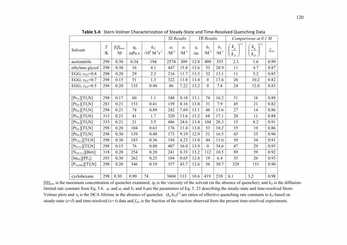
120
Table 5.4: Stern‐Volmer Characterization of Steady‐State and Time‐Resolved Quenching Data
SS Results TR Results Comparisons at 0.1 M
Solvent T /K
[Q]max /M
mPa s
kD /108 M-1s-1
a2 /M-2
a1 /M-1
0 /ns
b2 /M-2
b1 /M-1
)( I
D
q
k
k
)(
D
q
k
kfobs
acetonitrile 298 0.30 0.34 194 2574 309 12.8 409 355 2.3 1.6 0.99ethylene glycol 298 0.30 16 4.1 447 15.8 13.6 53 20.9 11 4.7 0.87EGG; xEG=0.8 298 0.20 29 2.3 216 11.7 13.5 32 13.1 11 5.2 0.85EGG; xEG=0.7 298 0.15 51 1.3 322 11.8 13.4 0 17.6 26 10.2 0.82EGG; xEG=0.5 298 0.20 135 0.49 86 7.22 13.2 0 7.8 24 12.0 0.83
[Pr31][Tf2N] 298 0.17 60 1.1 348 9.18 13.1 74 16.2 31 16 0.89[Pr41][Tf2N] 283 0.21 153 0.41 159 8.16 13.0 31 7.9 45 21 0.82[Pr41][Tf2N] 298 0.21 74 0.89 242 7.69 13.1 48 11.6 27 14 0.86[Pr41][Tf2N] 313 0.21 41 1.7 320 13.6 13.2 68 17.1 20 11 0.88[Pr41][Tf2N] 333 0.21 21 3.5 486 24.6 13.4 104 28.3 15 8.2 0.91[Pr61][Tf2N] 298 0.20 104 0.63 176 11.4 13.0 53 10.2 35 19 0.86[Pr81][Tf2N] 298 0.30 139 0.48 173 9.19 12.9 51 16.5 43 35 0.96[Pr10,1][Tf2N] 298 0.30 183 0.36 194 4.23 13.0 44 11.6 50 34 0.91[N3111][Tf2N] 298 0.15 76 0.88 407 16.0 13.9 0 34.6 47 29 0.93[N10,111][Beti] 318 0.20 254 0.28 241 8.33 13.2 112 10.5 89 59 0.92[Im41][PF6] 293 0.30 262 0.25 104 0.65 12.8 19 6.4 35 26 0.93[P14,666][Tf2N] 298 0.20 346 0.19 357 43.7 12.6 56 30.7 329 151 0.90 cyclohexane 298 0.30 0.90 74 3604 113 10.6 419 210 6.1 3.2 0.98
[Q]max is the maximum concentration of quencher examined, 0 is the viscosity of the solvent (in the absence of quencher), and kD is the diffusion-limited rate constant from Eq. 5.6. a1 and a2 and b1 and b2are the parameters of Eq. 5. 23 describing the steady-state and time-resolved Stern-
Volmer plots and 0 is the DCA lifetime in the absence of quencher. (kq/kD)(x) are ratios of effective quenching rate constants to kD based on
steady-state (x=I) and time-resolved (x=) data and fobs is the fraction of the reaction observed from the present time-resolved experiments.

121
Figure 5.4: Correlation between the ratio of quenching rate constants kq obtained from Stern‐
Volmer plots at 0.1 M DMA to diffusion‐controlled rate constant kD. Filled and open symbols
denote data in conventional solvents and ionic liquids respectively. Circles are data from
steady‐state intensity measurements (I0/I) and diamonds are data from integral decay times (
/0 ).
Viscosity / mPa s
10-1 100 101 102 103
k q/k D
100
101
102
I IL
conv

122
Before discussing this analysis it is useful to consider the meaning of the
differences in the Stern-Volmer plots obtained from steady-state versus time-resolved
measurements. As already noted, the extent of quenching reported by steady-state
measurements is generally larger, which indicates that some portion of the quenching is
missed by the time-resolved experiments, presumably due to insufficient time resolution
of the TCSPC experiment. As shown in Fig. 5.3 the difference between I0/I and /0 is
greater than a factor of 2 at the higher concentrations of quencher. Such large differences
might be interpreted to mean that a substantial fraction of the reaction is too fast to be
observed in the present experiments. But this is not the case. The two experiments report
the fraction of molecules that are quenched prior to emission as
0
)( 1I
If I
q and 0
)( 1 qf (5.24)
The fraction of the molecules initially excited but not observed in the time-resolved
experiments (the so-called “static” quenching component25) is the difference
)()( q
Iqstatic fff . The fraction of excited molecules that are observed is thus
00
1
I
Ifobs (5.25)
This fraction is listed in the last column of Table 5.4. The fobs values listed correspond to
0.1 M quencher but values are similar at other concentrations. In case is fobs< 0.8; it
averages 0.91 over the data set examined here. The ~25 ps resolution of the TCSPC
technique does not preclude accurately fitting the quenching data obtained here as long as
this missing fraction is accounted for.

123
5.4.2. Fitting to the Reaction Model
Rather than directly fitting the observed time-resolved decays to the reaction
model, we instead used the multi-exponential representations of the decay data such as
those shown in Table 5.3. Data sets for each solvent and temperature were fit separately,
with most sets consisting of five quencher concentrations of approximately 0, 0.05, 0.1,
0.15, 0.2 M. The multi-exponential parameterizations of these data were used to create
samples of 200 points equally spaced between 100 ps and the time at which the
fluorescence dropped to 1% of its initial intensity (1-50 ns) for each quencher
concentration. The starting time of 100 ps was chosen as the point where the effects of
instrumental broadening were expected to be negligible after multi-exponential fitting.
To account for the fact that some of the early decay was missed due to limited time
resolution, each sampled decay was normalized using the value of fobs determined from
the differences between I0/I and0/<> as described in the previous section. In addition to
the decay data, figure 5.5 shows how the viscosity data are interpolated. Figure 5.5a
shows some representative plots. All the ionic liquids and other solvents studied here are
treated in the same way as these plots. The estimation of the solution viscosities as
functions of composition were supplied as what is shown in figure 5.5b. The data in
Table 5.5 shows that at 0.3 M concentration DMA induces a decrease of ~ 24% in the
viscosities of the ionic liquids studied. In the highest viscosity conventional solvent used
for quenching experiments, 50 mole percent ethylene glycol + glycerol, the change is
only 5% and it is expected to be smaller in the conventional solvents of lower viscosity.

124
Figure 5.5: VFT fitting (eq. 5.7). (a): The mixtures of ethylene glycol and glycerol. Points are measured data and smooth curves the VFT fits. (b): Viscosities of [Pr41][Tf2N] and a 50 mole percent mixture of ethylene glycol + glycerol mixture without (filled symbols) and with (open symbols) 0.3 M DMA added.
T / K
290 300 310 320 330 340 350
ln(
/cP
)
1.0
2.0
3.0
4.0
5.0
6.0
7.0
8.0
x(EG)
00.3
0.5
0.70.8
T / K
280 290 300 310 320 330 340
ln(
/cP
)
3.0
3.5
4.0
4.5
5.0
5.5
Pr41
EG+gly

125
Table 5.5: Summary of Temperature‐Dependent Fits to Viscosity Data
Neat Solvents
Solvent Range/K A B T0/K T/K (T)
[Pr31][Tf2N] 278‐338 ‐1.90 839 158 298 60
[Pr41][Tf2N] 278‐338 ‐3.14 1266 128 298 74
[Pr61][Tf2N] 278‐338 ‐1.92 875 166 298 109
[Pr81][Tf2N] 278‐338 ‐1.91 887 168 298 139
[Pr10,1][Tf2N] 278‐338 ‐2.34 1028 162 298 183
[N3111][Tf2N] 293‐333 ‐0.78 563 190 298 82
[N10,111][Beti] 308‐343 ‐2.58 988 197 318 254
[Im41][PF6] 283‐337 ‐1.88 879 177 293 300
[P14,666][Tf2N] 288‐338 ‐3.10 1389 143 298 346
EGG; xEG=0.8 293‐338 ‐3.27 815 175 298 29
EGG; xEG=0.7 308‐338 ‐3.05 781 185 298 46
EGG; xEG=0.5 293‐338 ‐6.85 2293 103 298 137
EGG; xEG=0.3 293‐333 ‐4.96 1620 146 298 288
glycerol 293‐338 ‐4.09 1346 176 298 982
With Added DMA
Solvent [DMA] A B T0/K (T) %
[Pr31][Tf2N] 0.30 ‐2.44 925 153 50 ‐17%
[Pr41][Tf2N] 0.30 ‐0.72 516 192 62 ‐17%
[Pr61][Tf2N] 0.30 ‐2.88 1029 154 70 ‐36%
[Pr81][Tf2N] 0.30 ‐2.58 979 162 102 ‐26%
[Pr10,1][Tf2N] 0.30 ‐3.09 1145 154 126 ‐31%

126
[N3111][Tf2N] 0.29 ‐2.40 983 150 68 ‐17%
[Im41][PF6] 1.12 ‐2.57 983 167 181 ‐40%
[P14,666][Tf2N] 0.20 ‐4.10 1635 129 270 ‐22%
EGG; xEG=0.5 0.19 ‐4.16 1298 154 130 ‐5%
Notes: “Range” specifies the temperature range of the data, A, B, and T0 are
parameters in Eq.5.7 KTT
BA
/)(cP)/ln(
0 , T is the temperature
at which quenching experiments were conducted, (T) the fitted viscosity at
that temperature and % the percent change in viscosity caused by the added DMA.
Fits were performed using programs written in Matlab using the nonlinear
optimization routine “lsqnonlin” provided with this software.80 The sum of the squared
residuals (r2) in the fitted and normalized data sets was used as the fit criterion for
minimization. For fitting purposes, most of the twelve model parameters summarized in
Table 5.2 were fixed at the known or assumed values as described in Sec. 5.3.2. The five
parameters V0, el, G0, FQ, and Rh were considered for fitting the model to the
experimental data. The electron transfer parameters V0, el, and G0 are strongly coupled
and are not sufficiently constrained by the data to be independently varied. As already
discussed, el was fixed at the estimate of 1.5 Å-1, despite the fact that it could depend
upon solvent. V0 represents an orientationally-averaged value which cannot be predicted
with any certainty, but it is reasonably assumed to be solvent independent. Fixing G0 to
-1.2 eV and allowing V0 to vary led to best-fit values in the range 40 V0200 cm-1 and
we chose an average value of V0= 100 cm-1 for all solvents. With these two parameters
fixed, variation of G0 primarily changes the overall rate of the electron transfer reaction.

127
The interplay between the electron transfer rate and the rate of diffusion, represented by
the second variable parameter Rh, is the main determinant of the shapes of the
fluorescence decays. The final variable parameter FQ, which describes the F-Q potential
of mean force, determines the relative concentration of quencher near to the fluorophore
at time zero. It enables some adjustment of the relative rates of reaction at short and long
times.To fit a given set of data we began with V0 = 100 cm-1, el = 1.5 Å-1,G0 = -1.2 eV
(or +0.8 eV for cyclohexane), and FQ = 2.5 kJ/mol, and varied only Rh. Then, separate
and simultaneous variations of FQ and G0 were attempted. If the value of r2 didn’t
decrease by more than 25% by optimizing one of these latter parameters, the constrained
value was adopted.

128
Table 5.6: Summary of Fit Results
T /K
0 /mPa
s
G0 /eV
FQ
/kJ mol-1
Rh /Å
r2 /10-
5
DDMA /10-11 m2 s-
1 Dobs/DSE Rest/Rh
acetonitrile 298 0.34 -1.2 4.7 0.65 0.4 323 1.6 2.6 ethylene glycol 298 16 -1.2 1.3 0.74 3.5 8.2 1.9 2.3 EGG; xEG=0.8 298 29 -1.2 2.5 0.97 3.6 3.9 1.6 1.7 EGG; xEG=0.7(a) 298 51 -1.2 3.8 0.67 1.9 2.7 2.0 2.5
EGG; xEG=0.5(a) 298 135 -1.2 5.1 0.79 2.1 1.3 2.5 2.1
[Pr31][Tf2N] 298 60 -1.2 1.4 0.46 3.7 1.7 3.2 3.7 [Pr41][Tf2N] 283 153 -1.2 2.9 0.31 3.8 3.0 5.5(b)
[Pr41][Tf2N] 298 74 -1.2 2.2 0.37 1.9 1.4 3.4 4.6 [Pr41][Tf2N] 313 41 -1.2 1.5 0.37 1.7 3.7 4.5(b)
[Pr41][Tf2N] 333 21 -1.2 1.0 0.37 1.4 4.2 4.5(b)
[Pr61][Tf2N] 298 104 -0.97 4.0 0.36 2.0 1.0 5.3 4.7 -1.2 2.5 0.29 2.6 [Pr10,1][Tf2N] 298 183 -0.97 3.9 0.24 2.9 0.57 6.3 7.0 -1.2 2.5 0.20 3.3 [N3111][Tf2N] 298 76 -0.87 5.8 0.23 2.7 7.2 -1.2 3.1 0.18 3.9 [N10,111][Beti] 318 254 -0.87 6.5 0.17 0.2 2.9 14 9.7 -1.2 4.0 0.11 2.6 [Im41][PF6] 293 262 -0.89 5.0 0.37 2.5 1.4 5.2 4.5 -1.2 3.5 0.27 4.3 [P14,666][Tf2N] 298 346 -0.96 5.4 0.070 2.9 3.0 15 24 -1.2 3.7 0.055 4.6 cyclohexane 298 0.90 0.80 6.5 0.67 13 163 2.1 2.5 0.80 6.6 1.13 4.2
V0, el, G0, FQ, and Rh are the model parameters described in Sec. 3 and Table 1. Values in
parenthesis indicate values held constant in the fitting (in addition to V0 and el.) r2 is the mean
squared residual of the fit, NyyrN
i
fiti
obsi /)(
1
22
. Dobs/DSE is the ratio of the measured
diffusion coefficient of DMA to the Stokes-Einstein prediction RTkD B 6/ .Rest/Rh is the
corresponding ratio of the estimated effective diffusion radius Å 68.1)( 111 QFest RRR and
the value Rh determined from fitting the quenching data (Eq. 5. 22). (a) The data for the xEG =0.7 and 0.5 mixtures only extend to 0.15 M in DMA due to its limited solubility. (b) values estimated from temperature-dependent diffusion data on solutes other than DMA.

129
Representative fits to the model of Sec. 5.3 are shown in Figs. 5.6 and 5.7, and a
summary of resulting model parameters is provided in Table 5.6. The two data sets in
Fig. 5.6 illustrate the quality of the fits achieved for ionic liquid solvents. According to
the values of the goodness of fit metric (r2, Table 5.6) these two limiting temperatures of
the [Pr41][Tf2N] series represent the best (333 K) and worst (283 K) fits achieved. The
first thing to be noted is that even in the best cases, the fits do not capture the
deconvoluted and sampled experimental data to within uncertainties. (We estimate a
value r2 310-6 would indicate such a fit.) Some of this imperfect fit can be ascribed to
inaccuracies in the measured quencher concentrations and in estimates of fobs, both of
which have an important impact on the value of r2. This problem can be seen in the 333
K data in Fig. 5.6 where the fit of one particular decay ([DMA] = 0.05 M) appears to be
incorrect by a small factor. For this decay the measured value of fobs is 0.91. Changing
this value to 0.95 i.e. rescaling the experimental data at this particular quencher
concentration by 4%, produces good agreement between all of the model and observed
decays and reduces r2 by a factor of four, without causing an appreciable change in the fit
parameters. Given that uncertainties in fobs are expected to be on the order of a few
percent, it is clear that some deviations between the model fits and the experimental data
can be attributed to inaccuracies in the estimates of fobs. But it is also clear that the model
does not provide a perfect representation of the experimental data. For example, in Table
5.6 one sees that the value of r2 increases systematically with decreasing temperature in
the [Pr41][Tf2N] series. Lowering temperature slows diffusion and the overall rate of the
quenching reaction and increases the non-exponentiality of the fluorescence decays. As
illustrated by the 283 K data, the increasing non-exponentiality of the emission decays

130
with increasing quencher concentration is captured by the model, but deviations from
experiment are larger than expected uncertainties even if one considers concentration
uncertainties allows for some rescaling of the decays to account for fobs inaccuracies.
Similar observations can be made of all of the other quenching data in polar
solvents. The ethylene glycol data in Fig. 5.7 provides another typical example. Thus,
we find that the model presented in Sec. 3 provides a good albeit imperfect description of
the quenching data in high polarity solvents. The same is not true of the cyclohexane
data. As shown in Fig. 5.7, in this solvent the concentration dependence of the decays is
poorly reproduced. We note that simply by adjusting the concentration of the 0.2 M data
by ~20% leads to an acceptable fit (data in parenthesis in Table 5.6) suggesting that
DMA association in this nonpolar solvent might be important. But more study is
necessary to determine the real cause of this deviation.

131
Figure 5.6: Fits of time‐resolved DCA decays in [Pr41][Tf2N] with different [DMA] at 283 K (left
panels) and 333 K (right panels). Sampled data are shown as crosses and the fits (Table 4) solid
curves. These two data sets represent some of the worst (283 K; r2=410‐5) and best (333 K; r2=110‐5) fits among the ionic liquids studied.
333 K
0 10 20 30
Time / ns0.1 1 10
Nor
mal
ized
Int
ensi
ty
0.0
0.2
0.4
0.6
0.8
1.0
0.1 1 10
283 K
0 10 20 30 4010-2
10-1
100
(r2=3.8) (r2=1.4)

132
Figure 5.7: Fits of DCA quenching data with different [DMA] in cyclohexane (left panels) and
ethylene glycol (right panels) at 25 C. Sampled data are shown as crosses and the fits (Table
5.4) solid curves.
We now consider whether the model parameters derived from these fits (Table
5.6) are physically reasonable, restricting attention to the polar solvent results. As shown
in Table 5.6, reasonable fits are achieved in most cases using the estimated value G0= -
EG
0 5 10 15 20
Time / ns0.1 1
Nor
mal
ized
Int
ensi
ty
0.0
0.2
0.4
0.6
0.8
1.0
0.1 1 10
chex
0 1 2 310-2
10-1
100
(r2=13)
(r2=3.5)
133
1.2 eV accompanied by values of FQ which average 2.9 kJ/mol. The latter values are
near to kBT as anticipated. We note that in the series of ethylene glycol + glycerol
mixtures and in the [Pr41][Tf2N] temperature series the value of FQ increases
systematically with increasing viscosity. Rather than indicating a real change in the F-Q
potential of mean force, this systematic variation probably reflects some shortcoming of
the model. In addition, the quenching data in a number of the ionic liquid solvents are
better fit with a smaller value of G0 near -0.9 eV with concomitantly higher values of
FQ. (G0 and FQ are strongly correlated in these fits.) Variation of G0 by 0.3 eV is
larger than expected for these ionic liquids and these better fits coupled to unrealistically
high values of FQ, are also likely due to imperfections in the description of the quenching
reaction. The final parameter Rh, which is well determined by the fits, fixes the
relationship between the solution viscosity and the relative F-Q diffusion coefficient.
Fitted values of Rh are all smaller than the value estimated from the radii of F and Q, Rest
=1.68 Å. There is also a clear distinction between the values of Rh in conventional and
ionic liquid solvents. In conventional solvents the ratio Rest/Rh~ 2(final column of Table
5.6) whereas in ionic liquids this ratio is typically between 4-7 with some values, such as
that in [P14,666][Tf2N], being much larger.
To explore whether the latter differences are actually related to differences in
solute diffusion or are simply fitting artifacts, we have measured tracer diffusion
coefficients of DMA in all of these solvents. The results are also provided in Table 5.6
along with the values of Dobs/DSE, the ratios of the measured DMA diffusion coefficients
to those estimated from the Stokes-Einstein (SE) equation, RTkD BSE 6/ . As shown
in Table 5.6 the ratios Dobs/DSE and Rest/Rh parallel one another in the different solvent

134
types; in conventional solvents Dobs/DSE~ 2 whereas larger values are found in ionic
liquids. Overall we find SEobshest DDRR /)3.02.1(/ independent of solvent type.
Thus, the variations in Rh obtained by fitting the quenching data do appear to reflect the
relative F-Q diffusion coefficients in different solvents and the fact that RhRest is
primarily a result of the inaccuracy of the SE equation. In a related study of solute
diffusion24 we show that Dobs/DSE increases as a function of the solvent-to-solute size
ratio. The fact that values of Rest/Rh and Dobs/DSE are larger in ionic liquids than in
conventional solvents can thus be attributed to fact that ionic liquid ions are typically
larger than molecules of many conventional organic solvents. Although we didn’t
measure diffusion coefficients of the fluorophore here, measurements of similar
molecules show that similar ratios of Dobs/DSE should pertain to DCA as well as DMA.
The foregoing discussion indicates that the model employed here provides a
sound, albeit imperfect, description of the quenching of DCA by DMA. In most cases the
concentration-dependent shapes of the decay curves are reasonably reproduced in both
conventional and ionic liquid solvents using a consistent and reasonable set of electron
transfer parameters. In addition, the relative diffusion coefficients derived from these
fits, as embodied in the effective hydrodynamic radius Rh, are consistent with
independently measured solute diffusion coefficients. It is the case that deviations
between the observed and fitted decays are often larger than experimental uncertainties,
even after accounting for the effect of uncertainties in fobs. It seems likely that better
agreement with experiment could be achieved through refinement of the model, for
example by considering more sophisticated theories of the electron transfer process, an
improved description of the F-Q distribution function, or inclusion of a distance-

135
dependent diffusion coefficient to account for hydrodynamic interactions between F and
Q. Evaluation of such improvements, which would benefit from measurements able to
capture the early dynamics (<100 ps) not monitored here, are reserved for future studies.
For now, we are satisfied that the present model is sufficiently realistic provide insight
into the nature of the DCA+DMA reaction and help explain the “anomalous” kinetics
exhibited by this and similar reactions in ionic liquids.
5.4.3. Interpretation of the DCA+DMA Reaction
Figure 5.8 shows the distance dependence of the electron transfer parameters G,
, Vel, }4/)(exp{ 2 TkG B (labeled “Ea”) and the total electron transfer rate
constant . Solid curves correspond to the model as applied to polar solvents and dashed
curves to cyclohexane. As a result of the way in which the relative permittivity enters
Eq. 5.17, the reaction free energy G depends little upon reactant separation in polar
solvents whereas it is strongly dependent on r in cyclohexane (Fig. 5.8a). Just the
opposite behavior occurs for the reorganization energy , which has zero solvent
contribution in the case of cyclohexane. In both cases 0 G at all accessible values
of r, meaning that electron transfer always occurs in the normal regime. Because of the
much smaller value of in cyclohexane, the activation energy term
}4/)(exp{ 2 TkG B exhibits a much steeper distance dependence than in polar
solvents and is nearly equal in importance to the coupling term Vel2 (Fig. 5.8b). As a
result, the net distance dependence of the electron transfer rate constant (r) is
considerably steeper in the case of cyclohexane. (r) decreases approximately

136
exponentially with decay constants of 1.9 and 3.0 Å-1 in polar solvents and cyclohexane
respectively (Fig. 5.8c). For both types of solvent is predicted to achieve a rate
constant of ~1 ps-1 near contact. Finally, Fig. 5.8d illustrates F-Q distributions spanning
the range of values of FQ obtained from the fits. We note that for values of FQ as large
as 5 kJ/mol (~2kBT here at 298K) the enhanced probability of finding an F-Q pair near
contact (gFQ~8) seems unrealistic. Such values, which are obtained in several of the fits
in Table 5.6 probably, reflect some error in the model representation at early times.

137
Figure 5.8: Some features of the electron transfer model applied here: (a) G(r) and (r) (Eqs. 5.16, 5.17); (b) the normalized exponential terms associated with the activation energy (“Ea”, eq.
5.14) and the electronic coupling (“Vel2”, Eq. 5.15); (c) complete electron transfer rate constant.
Solid curves show the model as applied to polar solvents and dashed curves the model for
cyclohexane using the parameters specified in Table 2. (d) F‐Q radial distribution functions (Eq.
5.21) of the model with values of the energy parameter FQ = 1.2, 2.5, and 5 kJ/mol at 298 K.
Finally, Fig. 5.9 uses “standard parameters” for polar solvents as listed in Table
5.2 to illustrate the effect of changing viscosity on the time-dependent reaction rate
coefficient k(t) and the fluorescence decay profiles I(t)/I(0). The latter are shown for a
quencher concentration of 0.1 M. At times sufficiently short that no reactant motion has
- G
,
/ eV
0
1
2
3
r / Å8 10 12 14
10-4
10-3
10-2
10-1
100
/ s
-1106
107
108
109
1010
1011
1012
G
G
(d)
r / Å8 10 12 14
g FQ( r
)
1
10
(a)
(b)
(c)
Vel2
Ea
Ea
5
2
1
polar
chex
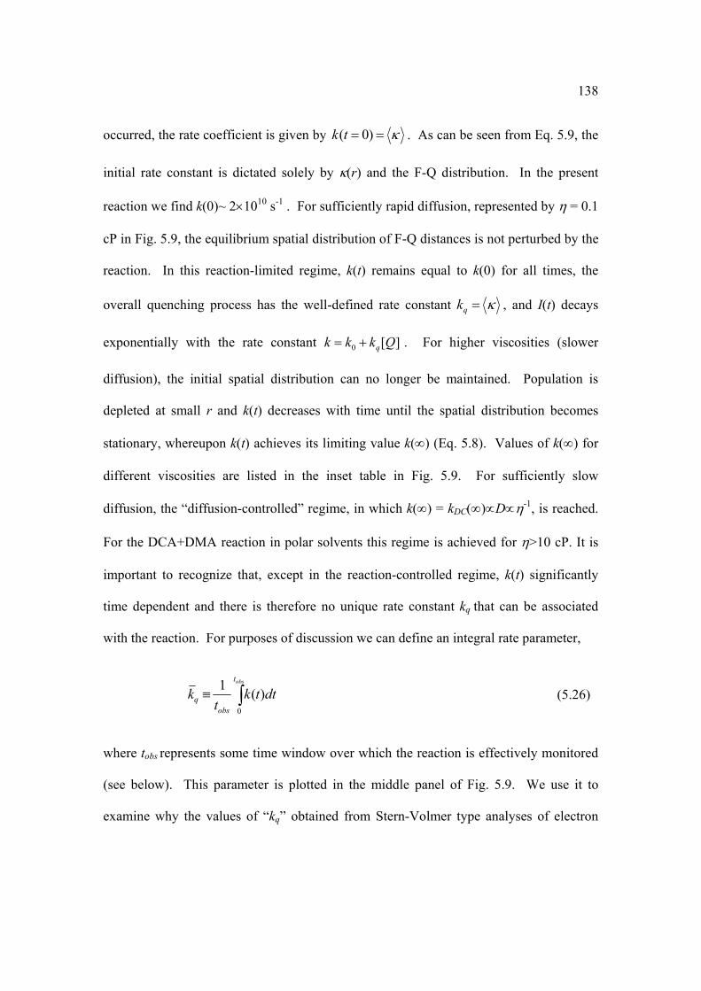
138
occurred, the rate coefficient is given by )0(tk . As can be seen from Eq. 5.9, the
initial rate constant is dictated solely by (r) and the F-Q distribution. In the present
reaction we find k(0)~ 21010 s-1 . For sufficiently rapid diffusion, represented by = 0.1
cP in Fig. 5.9, the equilibrium spatial distribution of F-Q distances is not perturbed by the
reaction. In this reaction-limited regime, k(t) remains equal to k(0) for all times, the
overall quenching process has the well-defined rate constant qk , and I(t) decays
exponentially with the rate constant ][0 Qkkk q . For higher viscosities (slower
diffusion), the initial spatial distribution can no longer be maintained. Population is
depleted at small r and k(t) decreases with time until the spatial distribution becomes
stationary, whereupon k(t) achieves its limiting value k() (Eq. 5.8). Values of k() for
different viscosities are listed in the inset table in Fig. 5.9. For sufficiently slow
diffusion, the “diffusion-controlled” regime, in which k() = kDC()D-1, is reached.
For the DCA+DMA reaction in polar solvents this regime is achieved for >10 cP. It is
important to recognize that, except in the reaction-controlled regime, k(t) significantly
time dependent and there is therefore no unique rate constant kq that can be associated
with the reaction. For purposes of discussion we can define an integral rate parameter,
obst
obsq dttk
tk
0
)(1
(5.26)
where tobs represents some time window over which the reaction is effectively monitored
(see below). This parameter is plotted in the middle panel of Fig. 5.9. We use it to
examine why the values of “kq” obtained from Stern-Volmer type analyses of electron

139
transfer reactions are often much larger than the simple Smoluchowski prediction
3/8 Tkk BD in ionic liquids.
The model of the DCA+DMA reaction developed here indicates that there are
multiple contributions which conspire to cause the large values of kq/kD shown in Table
5.4. As a representative example, we consider [Pr61][Tf2N], which has a viscosity of
~100 cP at 298 K. As listed in Table 5.4, Stern-Volmer analysis of the steady-state
quenching data yields the value kq/kD= 35 at 0.1 M DMA for this case. The first
contribution to this underestimation of kq relates to the fact that the reaction model
assumed in the simple Smoluchowski prediction for kD differs from the reaction model
adopted here. The simple Smoluchowski approach assumes negligible F-Q interactions,
i.e. w(r) = 0 for r>RF+RQ, and also assumes infinitely rapid reaction at contact but no
reaction elsewhere. Inclusion of a non-zero w(r) and a finite, distance-dependent (r) in
the more complete model used here leads to the differences between k() and kD shown
in the inset table in Fig. 5.9. In the diffusion-controlled regime, which pertains to
[Pr61][Tf2N], these differences in reaction model only increase k() over kD by a modest
34%. A second, and more important source of error in kD is the inaccuracy of the Stokes-
Einstein equation for predicting diffusion coefficients in ionic liquids. The value of
Dobs/DSE = 5.3 (Table 5.6) indicates that use of this hydrodynamic approximation results
in a value of kD which is about 5-fold smaller than what would be obtained using
measured diffusion coefficients. (As mentioned previously, the large size of ionic liquid
constituents makes this contribution to kq/kD much larger in ionic liquids than in many
conventional solvents.) A final source of error lies in the fact that kD is only an estimate
for the long-time limiting rate constant pertaining after the F-Q distribution has become

140
stationary. By comparing Stern-Volmer quenching data to kD one implicitly assumes that
little or no quenching occurs during the “transient” portion of the reaction. Such an
assumption is typically incorrect. In the present systems a substantial portion of the
quenching occurs before a stationary distribution has been established. When k(0) and
k() differ substantially, as they do here for viscosities greater than 10 cP (Fig. 5.9), non-
exponential decays and net quenching efficiencies much greater than predicted from kD or
k() are expected. For example, the effective quenching rate “constants”kq used in
compiling (kq/kD)(I) values in Table 5.4 are defined by ])[/()1( 00 QI
Ikq . Such kq
values, determined from model I(t)/I(0) decays for a quencher concentration of 0.1 M, are
listed in the inset table to Fig. 5.9. At a viscosity of 100 cP, which pertains to the
[Pr61][Tf2N] case, )(/ kkq =4.6. Thus, in this example, the error in the simple
Smoluchowski prediction for the extent of reaction kq/kD~ 35, can be thought of as
resulting from a product of three factors: (i) a modest factor of ~1.3 due to neglect of a
non-uniform initial F-Q distribution and the distance dependence of reaction (ii) a factor
of ~5 error due to inaccuracy of the SE prediction of diffusion coefficients, and (iii)
another factor of ~5 error due to the fact that much of the reaction occurs during the non-
stationary regime.

141
Figure 5.9: Model calculations illustrating the dependence of the quenching reaction upon
solution viscosity (values in mPas). k(t) is the time‐dependent rate constant (Eq. 5.7), )(tkq is
the cumulative average of k(t) defined in Eq. 5.26, and I(t)/I(0) is the normalized fluorescence decay (Eq. 5.1). Parameter values are those appropriate to polar solvents listed in Table 2 with
[Q]=0.1 M and 0 = 13 ns. The crosses in the middle panel indicate effective observation
windows defined by ]/[)/1/1()( 0 Qtk obsq with
0
)0(/)( IdttI . The curve
labeled 0 is the decay in the absence of quencher. The inset table compares values of the
limiting rate constant at infinite time (k(); Eq. 5.8), the diffusion‐limited rate constant kD given
by Eq. 5.6, and the effective quenching rate constant ]/[)/1/1( 0 Qkq .
k(t)k(
t) /
M-1
s-1
108
109
1010
0.11 10 100 1000
I(t)
Time / ns10-3 10-2 10-1 100 101 102
I(t)
/I(0
)
0.2
0.4
0.6
0.8
1.0
kq(t)
k q(t)
/ M
-1 s
-1
108
109
1010
k() kD kq0.1 181 661 1911 64 66 9610 8.5 6.6 20100 0.88 0.66 4.01000 .088 .066 1.5
0

142
We finally ask how viscosity and other experimental variables influence the last
of these three sources of deviation in kq/kD and thereby offer some insight into the
literature data collected in Table 5.1. To do so it is helpful to define an effective time
window tobs over which quenching experiments monitor reaction. We define this time by
]/[)/1/1()( 0 Qtk obsq . Such times for [Q]=0.1 M are marked as crosses in the
middle panel of Fig. 5.9. From this figure one finds that with decreasing viscosity the
reaction becomes faster and tobs becomes shorter. With this truncation of the observation
window kq approaches k(0) and one might therefore expect kq to be even farther from the
diffusion-controlled limit k(). But, because the difference between k(0) and k()
lessens with decreasing viscosity, the net effect is to cause kq/k() to decrease relative to
its value at high viscosities. For this reason, equating kq to k() as is done in the simple
Smoluckowski approach, often appears to be a good approximation in low viscosity
solvents, it becomes progressively worse as viscosity increases. This effect is the
primary reason for the variation of kq/kD with as shown in Fig. 5.4. Quencher
concentration and fluorophore lifetime 0 also affect the observation window and thus
how much kq departs from k(). For =100 cP and [Q]=0.1M one finds that tobs~0, i.e. it
is the fluorophore lifetime that mainly limits the extent of reaction. For 0 = 1, 10, 100 ns
values of kq/k() = 19, 5, and 2. Thus, other things being equal, a longer-lived
fluorophore achieves effective quenching rates closer to the diffusion limit. If the
quencher concentration is increased beyond 0.1 M at = 100 cP, the reaction limits the
observation window. For example, changing [Q] from 0.1 M to 1 M causes the
observation window to decreases from ~11 ns to ~1 ns and kq/k() increases from 4.6 to
16.

143
These observations provide some insight into the wide range of values of kq/kD
listed in Table 5.1. First we note that for reactions measured in multiple ionic liquids
having widely differing viscosities (#5, 6, 7, 8, 10) values of kq/kD increase with
increasing viscosity similarly to what is shown in Fig. 5.4. Presumably the interpretation
of this behavior is the same as just described for the DCA+DMA reaction. For a number
of reactions examined in high viscosity ionic liquids (#6-10) values of kq/kD were found
to be modest, less than 10 in most cases. Common to these cases is the fact that
observations were made at low reactant concentrations and with reactants whose lifetimes
were relatively long. Under these conditions the observation window is not limited to
short times and the measurements do not tend to emphasize the transient portion of the
reaction. In contrast, extreme values of kq/kD(#1, 3, 5) are limited to high-viscosity
systems in which solute lifetimes and/or high concentrations tend to emphasize the short-
time portions of k(t) occurring well before stationary conditions apply. These
observations are also consistent with what would be expected based on the foregoing
analysis. One aspect of the data in Table 5.1 that seems contrary to expectations is the
difference between kq/kD in systems 2 and 3. These data are for quenching of coumarins
C151 and C152 by DMA in two different ionic liquids. These data were recorded by a
single research group using the same methods.20,21 It is difficult to rationalize why large
values of kq/kD should be observed in the moderate viscosity liquid (DAF) at relatively
low quencher concentrations when much more modest values are observe in
[Im21][Tf2N]. For example, using the model parameters in Table 5.2 with = 100 cP, 0
= 1 ns, and [Q] = 1 M and assuming Dobs/DSE ~5 one finds kq/kD ~ 200, comparable to the
most extreme values in Table 5.1. Thus, it seems reasonable to expect that detailed

144
analyses of the sort described here, taking into account the specifics of the electron
transfer processes involved as well as the underestimation of diffusion coefficients by
Stokes-Einstein predictions, would provide satisfactory explanations for what appear to
be widely variable and sometimes unexpectedly high reaction rates reported for
diffusion-limited reactions in ionic liquids.
5.5. Summary and Conclusions
We have studied the electron transfer reaction between S1 DCA and DMA using
steady-state and picosecond time-resolved emission techniques in ionic liquids and
conventional solvents. Our primary interest was to better understand why diffusion-
limited electron transfer reactions sometimes appear to be much faster than expected
based on viscosity scaling the rates observed in conventional solvents.
For the quencher concentrations examined here (0.05-0.3 M) emission decays
were typically found to be significantly non-exponential and Stern-Volmer plots of
steady-state intensities and (integral) lifetimes far from linear in ionic liquid solvents.
These features indicate that reaction does not involve a simple kinetic process.
Application of the usual Stern-Volmer(SV) analysis to such data provided results
qualitatively similar to what was reported by Vieira and Falvey19 for this particular
reaction and by others for other similar reactions. Even at concentrations of 0.1 M in
DMA, effective quenching rate “constants” kq were found to be much larger than the
simple Smoluchowski prediction for diffusion-limited reactions, 3/8 Tkk BD . Values
of kq/kD greater than 10 are typical with values greater than 100 observed in some cases.

145
But such large departures from the kD prediction are not a unique feature of ionic liquids.
We also observed kq>>kD in conventional solvents having viscosities comparable to those
of ionic liquids. Moreover, a general correlation between kq/kD and viscosity was noted.
The origin of these departures from kD predictions and, indeed, even the meaning of the
kq values obtained in this manner, is unclear without further analysis.
We therefore also considered a more complete description of the quenching
process, using a model that combines solution of a spherical diffusion equation coupled
to a Marcus-type description of the electron transfer reaction. Such modeling has been
applied to reactions in conventional solvents29,30 ,31-38 but had not yet been considered in
ionic liquids. Using this approach we were able to obtain satisfactory fits of the
concentration-dependent fluorescence decay profiles observed in both ionic liquids and
conventional solvents using a consistent set of physically reasonable parameters. The
model developed for the DCA+DMA reaction showed that there are two main reasons
why the kq values obtained from SV analysis are often much greater than kD in ionic
liquids and other high viscosity media. First, conditions of high viscosity (slow
diffusion) emphasize the “transient” portions of reaction, i.e. those portions occurring
prior to establishment of steady-state conditions where the rate coefficient k(t) is time-
dependent. The rate constant kD is only a prediction for the limiting time constant
)( tk , which is smaller than k(t) at any earlier time. Stern-Volmer analysis provides
an effective rate constant kq which can be viewed as an average of k(t) over some time
window set by a combination of the net quenching rate and fluorophore lifetime. kq is
therefore necessarily larger than k() whose estimate is kD. In high viscosity (> 100 cP)
solvents and for the conditions employed here we estimate that kq/k() is in the range of

146
5-10. Even larger values are expected for experiments conducted with higher quencher
concentrations and/or shorter fluorophore lifetimes. These considerations are the same
for ionic liquids and conventional solvents.
The second important contributor to large values of kq/kD is the fact that the
Stokes-Einstein relationship, RTkD BSE 6/ , used in deriving the simple
Smoluchowski prediction for kD, significantly underestimates diffusion coefficients in
ionic liquids. This effect was suggested by the small effective hydrodynamic radii
required to fit the quenching data to the model and also confirmed by direct
measurements of the diffusion coefficients of DMA in all of the solvents studied. Ratios
of Dobs/DSE in all solvents are in part a function of the relative sizes of solute and solvent
molecules. The fact that ionic liquid cations and anions are often larger than the
molecules of many conventional solvents makes such ratios larger in ionic liquids.
Values of 3-5 are typical in ionic liquids but values of Dobs/DSE larger than 10 are
observed for ionic liquids comprised of the largest cations studied. These diffusion
factors multiply the factors of kq/k() caused by transient effects so that together quite
large values of kq/kD are obtained.
We have only considered one particular reaction in this study and have applied
what can be viewed as a minimally realistic model for treating bimolecular electron
transfer reactions. Nevertheless, it seems likely that foregoing interpretations suffice to
account for other cases in which surprisingly large values of kq (i.e. kq>>kD) have been
reported. No special character of electron transfer need be postulated to explain such
observations. Furthermore, while solute diffusion is faster than what Stokes-Einstein
estimates in ionic liquids, values of Dobs/DSE are likely to be much smaller than the

147
extreme values of kq/kD observed. We therefore conclude that none of the studies
published to date offer clear evidence for bimolecular electron transfer rates being
anomalously high in ionic liquids.
Notes and References
1. J. F. Wishart, "Energy applications of ionic liquids," Energy & Environmental Science2, 956-961 (2009).
2. M. Armand, F. Endres, D. R. MacFarlane, H. Ohno, and B. Scrosati, "Ionic-liquid materials for the electrochemical challenges of the future," Nature Materials8, 621-629 (2009).
3. A. Lewandowski and A. Swiderska-Mocek, "Ionic liquids as electrolytes for Li-ion batteries: An overview of electrochemical studies," J. Power Sources194, 601-609 (2009).
4. P. Hapiot and C. Lagrost, "Electrochemical Reactivity in Room-Temperature Ionic Liquids," Chemical Reviews (Washington, DC, United States)108, 2238-2264 (2008).
5. L. E. Barrosse-Antle, A. M. Bond, R. G. Compton, A. M. O'Mahony, E. I. Rogers, and D. S. Silvester, "Voltammetry in room temperature ionic liquids: Comparisons and contrasts with conventional electrochemical solvents," Chem.--Asian J.5, 202-230 (2010).
6. D. E. Khoshtariya, T. D. Dolidze, and R. van Eldik, "Multiple Mechanisms for Electron Transfer at Metal/Self-Assembled Monolayer/Room-Temperature Ionic Liquid Junctions: Dynamical Arrest versus Frictional Control and Non-Adiabaticity," Chem.--Eur. J.15, 5254-5262, S5254/5251-S5254/5253 (2009).
7. F. Endres, O. Hoefft, N. Borisenko, L. H. Gasparotto, A. Prowald, R. Al-Salman, T. Carstens, R. Atkin, A. Bund, and E. A. S. Zein, "Do solvation layers of ionic liquids influence electrochemical reactions?," Phys. Chem. Chem. Phys.12, 1724-1732 (2010).
8. R. M. Lynden-Bell, "Can Marcus Theory Be Applied to Redox Processes in Ionic Liquids? A Comparative Simulation Study of Dimethylimidazolium Liquids and Acetonitrile," J. Phys. Chem. B111, 10800-10806 (2007).

148
9. Y. Shim and H. J. Kim, "Free Energy and Dynamics of Electron-Transfer Reactions in a Room Temperature Ionic Liquid," J. Phys. Chem. B111, 4510-4519 (2007).
10. Y. Shim and H. J. Kim, "Adiabatic Electron Transfer in a Room-Temperature Ionic Liquid: Reaction Dynamics and Kinetics," J. Phys. Chem. B113, 12964-12972 (2009).
11. H. V. R. Annapureddy and C. J. Margulis, "Controlling the outcome of electron transfer reactions in ionic liquids," J. Phys. Chem. B113, 12005-12012 (2009).
12. X. Li, M. Liang, A. Chakraborty, M. Kondo, and M. Maroncelli, "Solvent-Controlled Intramolecular Electron Transfer in Ionic Liquids," J. Phys. Chem. B115, 6592-6607 (2011).
13. A. Samanta, "Solvation Dynamics in Ionic Liquids: What We Have Learned from the Dynamic Fluorescence Stokes Shift Studies," Journal of Physical Chemistry Letters1, 1557-1562 (2010).
14. M. Maroncelli, X.-X. Zhang, M. Liang, D. Roy, and N. P. Ernsting, "Measurements of the complete solvation response of coumarin 153 in ionic liquids and the accuracy of simple dielectric continuum predictions," Faraday Discuss. Chem. Soc.154, in press (2012).
15. C. M. Gordon and A. J. McLean, "Photoelectron transfer from excited-state ruthenium(II) tris(bipyridyl) to methylviologen in an ionic liquid," Chem. Comm., 1395-1396 (2000).
16. A. J. McLean, M. J. Muldoon, C. M. Gordon, and I. R. Dunkin, "Bimolecular rate constants for diffusion in ionic liquids," Chem. Comm., 1880-1881 (2002).
17. A. Skrzypczak and P. Neta, "Diffusion-Controlled Electron-Transfer Reactions in Ionic Liquids," J. Phys. Chem. A107, 7800-7803 (2003).
18. G. Grampp, D. Kattnig, and B. Mladenova, "ESR-spectroscopy in ionic liquids: Dynamic line-broadening effects caused by electron-self exchange reactions within the methylviologene redox couple," SpectrochimicaActa, Part A: Molecular and Biomolecular Spectroscopy63A, 821-825 (2006).
19. R. C. Vieira and D. E. Falvey, "Photoinduced Electron-Transfer Reactions in Two Room-Temperature Ionic Liquids: 1-Butyl-3-methylimidazolium Hexafluorophosphate and 1-Octyl-3-methylimidazolium Hexafluorophosphate," J. Phys. Chem. B111, 5023-5029 (2007).
20. S. Sarkar, R. Pramanik, D. Seth, P. Setua, and N. Sarkar, "Photoinduced electron transfer (PET) from N,N-dimethylaniline to 7-amino Coumarin dyes in a room

149
temperature ionic liquid (RTIL): Slowing down of electron transfer rate compared to conventional solvent," Chem. Phys. Lett.477, 102-108 (2009).
21. S. Sarkar, R. Pramanik, C. Ghatak, V. G. Rao, and N. Sarkar, "Photoinduced intermolecular electron transfer in a room temperature imidazolium ionic liquid: An excitation wavelength dependence study," Chem. Phys. Lett.506, 211-216 (2011).
22. K. Takahashi, H. Tezuka, S. Kitamura, T. Satoh, and R. Katoh, "Reactions of excited-state benzophenoneketyl radical in a room-temperature ionic liquid," Physical chemistry chemical physics : PCCP12, 1963-1970 (2010).
23. A. K. Das, T. Mondal, M. S. Sen, and K. Bhattacharyya, "Marcus-like Inversion in Electron Transfer in Neat Ionic Liquid and Ionic Liquid-Mixed Micelles," J. Phys. Chem. B115, 4680-4688 (2011).
24. A. Kaintz, A. Benesi, G. Baker, and M. Maroncelli, "Solute Diffusion in a Series of Pyrrolidinium Ionic Liquids," manuscript in preparation (2012).
25. J. R. Lakowicz, Principles of Fluorescence Spectroscopy, 3rd ed. (Springer, New York, 2006).
26. A. Nitzan, Chemical Dynamics in Condensed Phases; Relaxation, Transfer, and Reactions in Condensed Molecular Systems (Oxford, New York, 2006).
27. A. Szabo, "Theory of diffusion-influenced fluorescence quenching," J. Phys. Chem.93, 6929-6939 (1989).
28. A. I. Burshtein, "Non-Markovian theories of transfer reactions in luminescence and chemiluminescence and photo- and electrochemistry," Adv. Chem. Phys.129, 105-418 (2004).
29. S. Murata, S. Y. Matsuzaki, and M. Tachiya, "Transient Effect in Fluorescence Quenching by Electron Transfer. 2. Determination of the Rate Parameters Involved in the Marcus Equation," J. Phys. Chem.99, 5354-5358 (1995).
30. S. Murata and M. Tachiya, "Transient Effect in Fluorescence Quenching by Electron Transfer. 3. Distribution of Electron Transfer Distance in Liquid and Solid Solutions," J. Phys. Chem.100, 4064-4070 (1996).
31. S. Iwai, S. Murata, and M. Tachiya, "Ultrafast fluorescence quenching by electron transfer and fluorescence from the second excited state of a charge transfer complex as studied by femtosecond up-conversion spectroscopy," J. Chem. Phys.109, 5963-5970 (1998).

150
32. L. Burel, M. Mostafavi, S. Murata, and M. Tachiya, "Transient effect in fluorescence quenching by electron transfer. 4. Long-range electron transfer in a nonpolar solvent," J. Phys. Chem. A103, 5882-5888 (1999).
33. S. F. Swallen, K. Weidemaier, H. L. Tavernier, and M. D. Fayer, "Experimental and Theoretical Analysis of Photoinduced Electron Transfer: Including the Role of Liquid Structure," J. Phys. Chem.100, 8106-8117 (1996).
34. S. F. Swallen, K. Weidemaier, and M. D. Fayer, "Solvent structure and hydrodynamic effects in photoinduced electron transfer," J. Chem. Phys.104, 2976-2986 (1996).
35. K. Weidemaier, H. L. Tavernier, S. F. Swallen, and M. D. Fayer, "Photoinduced Electron Transfer and Geminate Recombination in Liquids," J. Phys. Chem. A101, 1887-1902 (1997).
36. A. Rosspeintner, D. R. Kattnig, G. Angulo, S. Landgraf, G. Grampp, and A. Cuetos, "On the coherent description of diffusion-influenced fluorescence quenching experiments," Chem.--Eur. J.13, 6474-6483 (2007).
37. A. Rosspeintner, D. R. Kattnig, G. Angulo, S. Landgraf, and G. Grampp, "The Rehm-Weller experiment in view of distant electron transfer," Chem.--Eur. J.14, 6213-6221 (2008).
38. G. Angulo, D. R. Kattnig, A. Rosspeintner, G. Grampp, and E. Vauthey, "On the Coherent Description of Diffusion-Influenced Fluorescence Quenching Experiments II: Early Events," Chem. Eur. J.16, 2291-2299, S2291/2291-S2291/2296 (2010).
39. O. K. Dudko and A. Szabo, "Time-Dependent Rate Coefficients for Diffusion-Influenced Reactions with Centrosymmetric Potentials," J. Phys. Chem. B109, 5891-5894 (2005).
40. H. Jin, B. O'Hare, J. Dong, S. Arzhantsev, G. A. Baker, J. F. Wishart, A. Benesi, and M. Maroncelli, "Physical Properties of Ionic Liquids Consisting of the 1-Butyl-3-Methylimidazolium Cation with Various Anions and the Bis(trifluoromethylsulfonyl)imide Anion with Various Cations," J. Phys. Chem. B112, 81-92 (2008).
41. P. Kilaru, G. A. Baker, and P. Scovazzo, "Density and surface tension measurements of imidazolium-, quaternary phosphonium-, and ammonium-based room-temperature ionic liquids: data and correlations," Journal of Chemical & Engineering Data52, 2306-2314 (2007).

151
42. J. A. Gardecki and M. Maroncelli, "A Set of Secondary Emission Standards for Calibration of Spectral Responsivity in Emission Spectroscopy," Appl. Spectrosc.52, 1179-1189 (1998).
43. M. P. Heitz and M. Maroncelli, "Rotation of Solutes in Supercritical CO2: Are Rotation Times Anomalously Slow in the Near Critical Regime?," J. Phys. Chem. A101, 5852-5868 (1997).
44. D. Wu, A. Chen, and C. S. Johnson, Jr., "An improved diffusion-ordered spectroscopy experiment incorporating bipolar-gradient pulses," Journal of Magnetic Resonance, Series A115, 260-264 (1995).
45. E. B. Krissinel and N. Agmon, "Spherical symmetric diffusion problem," J. Comput. Chem.17, 1085-1098 (1996).
46. M. Smoluchowski, "Mathematical theory of the kinetics of the coagulation of colloidal solutions," Z. Physik. Chem.92, 129-168 (1917).
47. K. Laidler, Chemical Kinetics (HarperCollins, New York, 1987).
48. J. I. Steinfeld, J. S. Francisco, and W. L. Hase, Chemical Kinetics and Dynamics (Plenum Press, Englewood Cliffs, 1989).
49. A factor of 2 is missing in the expression for 1,2 given as Eq. 5.21c of Ref.39 Equation 11 is the corrected version. Attila Szabo, private communication.
50. R. A. Marcus and N. Sutin, "Electron Transfers in Chemistry and Biology," Biochim. Biophys. Acta811, 265-322 (1985).
51. A. V. Barzykin, P. A. Frantsuzov, K. Seki, and M. Tachiya, "Solvent effects in nonadiabatic electron-transfer reactions: Theoretical aspects," Adv. Chem. Phys.123, 511-616 (2002).
52. R. A. Marcus, "The theory of oxidation-reduction reactions involving electron transfer. I," J. Chem. Phys.24, 966-978 (1956).
53. K. Miyazaki and M. Tachiya, "Exact calculation of the solvation energy of a pair of ions in polar media within the framework of the dielectric continuum model," J. Chem. Phys.109, 7424-7430 (1998).
54. D. Rehm and A. Weller, "Kinetics of fluorescence quenching by electron and hydrogen-atom transfer," Isr. J. Chem.8, 259-271 (1970).
55. J. T. Edwards, "Molecular Volumes and the Stokes-Einstein Equation," J. Chem. Ed.47, 261-270 (1970).

152
56. E. W. J. Castner, D. Kennedy, and R. J. Cave, "Solvent as Electron Donor: Donor/Acceptor Electronic Coupling Is a Dynamical Variable," J. Phys. Chem. A104, 2869-2885 (2000).
57. P. O. J. Scherer, "Microscopic Models for Ultrafast Photoinduced Solvent to Dye Electron Transfer in DMA/Oxazine Solution," J. Phys. Chem. A104, 6301-6307 (2000).
58. P. O. J. Scherer and M. Tachiya, "Computer simulation studies of electron transfer parameters for cyanoanthracene/N,N-dimethylaniline solutions," J. Chem. Phys.118, 4149-4156 (2003).
59. O. S. Wenger, "How Donor-Bridge-Acceptor Energetics Influence Electron Tunneling Dynamics and Their Distance Dependences," Acc. Chem. Res.44, 25-35 (2011).
60. O. S. Wenger, B. S. Leigh, R. M. Villahermosa, H. B. Gray, and J. R. Winkler, "Electron Tunneling Through Organic Molecules in Frozen Glasses," Science (Washington, DC, U. S.)307, 99-102 (2005).
61. J. R. Miller, J. V. Beitz, and R. K. Huddleston, "Effect of free energy on rates of electron transfer between molecules," J. Am. Chem. Soc.106, 5057-5068 (1984).
62. J. Eriksen and C. S. Foote, "Electron-transfer fluorescence quenching and exciplexes of cyano-substituted anthracenes," J. Phys. Chem.82, 2659-2662 (1978).
63. I. R. Gould, D. Ege, J. E. Moser, and S. Farid, "Efficiencies of photoinduced electron-transfer reactions: role of the Marcus inverted region in return electron transfer within geminate radical-ion pairs," J. Am. Chem. Soc.112, 4290-4301 (1990).
64. K. Kikuchi, M. Hoshi, T. Niwa, Y. Takahashi, and T. Miyashi, "Heavy-atom effects on the excited singlet-state electron-transfer reaction," J. Phys. Chem.95, 38-42 (1991).
65. G. Jones, S. F. Griffin, C. Y. Choi, and W. R. Bergmark, "Electron donor-acceptor quenching and photoinduced electron transfer for coumarin dyes," The Journal of Organic Chemistry49, 2705-2708 (1984).
66. D. Burget, P. Jacques, E. Vauthey, P. Suppan, and E. Haselbach, "Marcus Inverted Region: Nature of Donor-Acceptor Pairs and Free Ion Yields," J. Chem. Soc. Faraday Trans.90, 2481-2487 (1994).

153
67. H. Shirota, H. Pal, K. Tominaga, and K. Yoshihara, "Substituent Effect and Deuterium Isotope Effect of Ultrafast Intermolecular Electron Transfer: Coumarin in Electron-Donating Solvent," J. Phys. Chem. A102, 3089-3102 (1998).
68. M.-M. Huang, Y. Jiang, P. Sasisanker, G. W. Driver, and H. Weingartner, "Static Relative Dielectric Permittivities of Ionic Liquids at 25 °C," Journal of Chemical & Engineering Data56, 1494-1499 (2011).
69. M. N. Kobrak and H. Li, "Electrostatic interactions in ionic liquids: the dangers of dipole and dielectric descriptions," Phys. Chem. Chem. Phys.12, 1922-1932 (2010).
70. C. F. Poole, "Chromatographic and spectroscopic methods for the determination of solvent properties of room temperature ionic liquids," Journal of Chromatography, A1037, 49-82 (2004).
71. C. Reichardt, "Polarity of ionic liquids determined empirically by means of solvatochromic N-phenolatebetaine dyes," Green Chem.7, 339-351 (2005).
72. W. E. Acree, Jr. and M. H. Abraham, "The analysis of solvation in ionic liquids and organic solvents using the Abraham linear free energy relationship," Journal of Chemical Technology and Biotechnology81, 1441-1446 (2006).
73. H. Jin, G. A. Baker, S. Arzhantsev, J. Dong, and M. Maroncelli, "Solvation and Rotational Dynamics of Coumarin 153 in Ionic Liquids: Comparisons to Conventional Solvents," J. Phys. Chem. B117, 7291-7302 (2007).
74. D. Roy and M. Maroncelli, "Solvation and Solvation Dynamics in an Idealized Ionic Liquid Model," manuscript in preparation (2011).
75. R. M. Lynden-Bell, "Redox potentials and screening in ionic liquids: Effects of sizes and shapes of solute ions," J. Chem. Phys.129, 204503/204501-204503/204507 (2008).
76. E. W. Castner, Jr, unpublished results (2011).
77. D. Roy and M. Maroncelli, "Solvation in an Idealized Ionic Liquid Model," manuscript in preparation (2011).
78. This observation of nonlinear Stern-Volmer plots is at odds with the results of Vieira and Falvey.19 These authors reported steady-state Stern-Volmer plots for the quenching of DCA by a variety of amines including DMA to be linear over concentration ranges of 0.4-1.2 M in [Im41][PF6] and [Im81][PF6]. We extended the measurements of DCA+DMA in [Im41][PF6] reported in Table 5.4 to the range 0.05 – 1.2 M in order to make more direct comparison to the Vieira and Falvey work but

154
found highly non-exponential Stern-Volmer plots. The reason for this discrepancy is not known.
79. Our value of (kq/kD) = 35 for the DCA+DMA reaction in [Im41][PF6] at 0.1 M DMA differs significantly from (kq/kD) = 85 calculated from the value of kq reported by Vieira and Falvey19 for this identical system. However, the latter authors measured quenching at higher DMA concentrations where the non-linearity of the Stern-Volmer plots makes the effective rate “constant” kq much larger.
80. For evaluating the complementary error function in Eq. 7, whose argument is often complex, we used a routine for numerical evaluation of the Faddeeva function
)()exp( 2 izerfcz described in J.A.C. Weideman, "Computation of the Complex Error Function," SIAM J. Numerical Analysis31, 1497-1518, (1994). The Matlab routine for this function was written by KeshIkuma and is available at http://www.mathworks.com/matlabcentral/fileexchange/22207-faddeeva-function-fft-based.
81. A. Paul and A. Samanta, "Photoinduced Electron Transfer Reaction in Room Temperature Ionic Liquids: A Combined Laser Flash Photolysis and Fluorescence Study," J. Phys. Chem. B111, 1957-1962 (2007).
82. K. Takahashi, S. Sakai, H. Tezuka, Y. Hiejima, Y. Katsumura, and M. Watanabe, "Reaction between Diiodide Anion Radicals in Ionic Liquids," J. Phys. Chem. B111, 4807-4811 (2007).

155
Vita
Min Liang
Education:
The Pennsylvania State University, University Park, PA USA (2007-present) Ph.D. candidate, Physical Chemistry Advisor: Professor Mark Maroncelli
Southeast University, Nanjing, P.R. China (2003-2006) M. S., Materials Physics and Chemistry Advisor: Professor Baoping Lin
Xinyang Normal University, Xinyang, P.R. China (1999-2003) B.S., Chemical Engineering Advisor: Associate Professor Fengtie Gui
Research Experience:
Fluorescence quenching studies of bimolecular electron transfer in ionic liquids
Complete solvation dynamics of Coumarin 153 in ionic liquids
Solvation dynamics of Coumarin 153 in the mixtures of an ionic liquid [Im41][BF4] with acetonitrile and water
Intramolecular electron transfer in ionic liquids
Photophysical characterization of benzylidene malononitriles as probes of solvent friction
Solvation studies on Brooker’s merocyanine
Production of ultrafine global silver powder applied in electronic materials
Awards and Honors: Miller Graduate Fellowship (2011-2012)
Travel award (2010-2011)
PSU Incoming Class New Graduate Student Award (2008-2009)
Braddock Graduate Fellowship (2007-2008)
Outstanding Graduate Student Fellowship (2005-2006)
Southeast University Graduate Student Fellowship (2003-2006)
Attended Conferences with Poster:
4th Congress on Ionic Liquids, Arlington, VA, June 15-18, 2011
239th ACS National Meeting, San Francisco, CA, March 21-25, 2010
238th ACS National Meeting, Washington, DC, August 16-20, 2009
236th ACS National Meeting, Philadelphia, PA, August 17-21, 2008

156
Professional Memberships:
American Chemical Society (2008-present)
Publications:
1. Liang, M.; Zhang, XX.; Ernsting, N.; Maroncelli, M., Solvation and Rotational Dynamics in a Prototypical Ionic Liquid + Dipolar Solvent Mixture. 2012.(manuscript in preparation)
2. Zhang, XX.; Liang, M.; Ernsting, N.; Maroncelli, M., The Complete Solvation Response of Coumarin 153 in Ionic Liquids. 2012. (manuscript in preparation)
3. Liang, M.; Kaintz, A.; Baker, G. A.; Maroncelli, M., Bimolecular Electron Transfer in Ionic Liquids: Are Reaction Rates Anomalously High? J. Phys. Chem. B 2012, 116, (4), 1370-1384.
4. Maroncelli, M. Zhang, XX,; Liang, M.; Roy, D. and Ernsting, N., Measurements of the Complete Solvation Response of Coumarin 153 in Ionic Liquids and the Accuracy of Simple Dielectric Continuum Predictions. Faraday Discussions 2011, 154.
5. Li, X.; Liang, M.; Chakraborty, A.; Kondo, M.; Maroncelli, M., Solvent-Controlled Intramolecular Electron Transfer in Ionic Liquids. J. Phys. Chem. B 2011, 115, (20), 6592-6607.
6. Jin, H.; Liang, M.; Arzhantsev, S.; Li, X.; Maroncelli, M., Photophysical Characterization of Benzylidene Malononitriles as Probes of Solvent Friction. J. Phys. Chem. B 2010, 114, (22), 7565-7578.
7. Liang, M.; Yennawar, H.; Maroncelli, M., 2-[(2,3,6,7-Tetrahydro-1H,5H-benzo[ij]quinolizin-9-yl)methylene]propanedinitrile. Acta Crystallogr., Sect. E: Struct. Rep. Online 2009, E65, (7), o1687.
8. Liang, M.; Tang, J.; Lin, B., Production of ultrafine global silver powder applied in electronic materials. Zhongguo Fenti Jishu 2006, 12, (3), 16-19, 47.
9. Lin, B.; Liang, M., Method for preparing spherical micron silver powders for conductive silver paste. Patent CN 1785558 A 20060614, 2006.