James R. DeBonisGlenn Research Center, Cleveland, Ohio

Solutions of the Taylor-Green Vortex Problem UsingHigh-Resolution Explicit Finite Difference Methods

NASA/TM—2013-217850

February 2013

https://ntrs.nasa.gov/search.jsp?R=20130011044 2018-05-19T21:22:42+00:00Z

NASA STI Program . . . in Profi le

Since its founding, NASA has been dedicated to the advancement of aeronautics and space science. The NASA Scientifi c and Technical Information (STI) program plays a key part in helping NASA maintain this important role.

The NASA STI Program operates under the auspices of the Agency Chief Information Offi cer. It collects, organizes, provides for archiving, and disseminates NASA’s STI. The NASA STI program provides access to the NASA Aeronautics and Space Database and its public interface, the NASA Technical Reports Server, thus providing one of the largest collections of aeronautical and space science STI in the world. Results are published in both non-NASA channels and by NASA in the NASA STI Report Series, which includes the following report types: • TECHNICAL PUBLICATION. Reports of

completed research or a major signifi cant phase of research that present the results of NASA programs and include extensive data or theoretical analysis. Includes compilations of signifi cant scientifi c and technical data and information deemed to be of continuing reference value. NASA counterpart of peer-reviewed formal professional papers but has less stringent limitations on manuscript length and extent of graphic presentations.

• TECHNICAL MEMORANDUM. Scientifi c

and technical fi ndings that are preliminary or of specialized interest, e.g., quick release reports, working papers, and bibliographies that contain minimal annotation. Does not contain extensive analysis.

• CONTRACTOR REPORT. Scientifi c and

technical fi ndings by NASA-sponsored contractors and grantees.

• CONFERENCE PUBLICATION. Collected papers from scientifi c and technical conferences, symposia, seminars, or other meetings sponsored or cosponsored by NASA.

• SPECIAL PUBLICATION. Scientifi c,

technical, or historical information from NASA programs, projects, and missions, often concerned with subjects having substantial public interest.

• TECHNICAL TRANSLATION. English-

language translations of foreign scientifi c and technical material pertinent to NASA’s mission.

Specialized services also include creating custom thesauri, building customized databases, organizing and publishing research results.

For more information about the NASA STI program, see the following:

• Access the NASA STI program home page at http://www.sti.nasa.gov

• E-mail your question to help@sti.nasa.gov • Fax your question to the NASA STI

Information Desk at 443–757–5803 • Phone the NASA STI Information Desk at 443–757–5802 • Write to:

STI Information Desk NASA Center for AeroSpace Information 7115 Standard Drive Hanover, MD 21076–1320

James R. DeBonisGlenn Research Center, Cleveland, Ohio

Solutions of the Taylor-Green Vortex Problem UsingHigh-Resolution Explicit Finite Difference Methods

NASA/TM—2013-217850

February 2013

National Aeronautics andSpace Administration

Glenn Research CenterCleveland, Ohio 44135

Prepared for the51st Aerospace Sciences Meetingsponsored by the American Institute of Aeronautics and AstronauticsGrapevine, Texas, January 7–10, 2013

Available from

NASA Center for Aerospace Information7115 Standard DriveHanover, MD 21076–1320

National Technical Information Service5301 Shawnee Road

Alexandria, VA 22312

Available electronically at http://www.sti.nasa.gov

This work was sponsored by the Fundamental Aeronautics Program at the NASA Glenn Research Center.

Level of Review: This material has been technically reviewed by technical management.

A computational fluid dynamics code that solves the compressible Navier-Stokes equa-tions was applied to the Taylor-Green vortex problem to examine the code’s ability to ac-curately simulate the vortex decay and subsequent turbulence. The code, WRLES (WaveResolving Large-Eddy Simulation), uses explicit central-differencing to compute the spatialderivatives and explicit Low Dispersion Runge-Kutta methods for the temporal discretiza-tion. The flow was first studied and characterized using Bogey & Bailley’s 13-point dis-persion relation preserving (DRP) scheme. The kinetic energy dissipation rate, computedboth directly and from the enstrophy field, vorticity contours, and the energy spectra areexamined. Results are in excellent agreement with a reference solution obtained using aspectral method and provide insight into computations of turbulent flows. In addition thefollowing studies were performed: a comparison of 4th-, 8th-, 12th- and DRP spatial dif-ferencing schemes, the effect of the solution filtering on the results, the effect of large-eddysimulation sub-grid scale models, and the effect of high-order discretization of the viscousterms.

Nomenclature

an spatial finite difference coefficientsbn spatial filter coefficientsc, c∗ actual and numerical wave speedet total energyp pressureqi heat flux vectort timet∗ nondimensional time, t∗ = t/(L/V0)ui velocity vectoru, v, w streamwise, transverse and spanwise velocity componentsx, y, z cartesian coordinatesD spatial finite difference operatorEk kinetic energyE(Ek) spectral density of kinetic energyL reference lengthM Mach numberRe Reynolds numberSij strain rate tensorSd

ij deviatoric strain rate tensor, Sdij = Sij − Skkδij

T temperatureV0 initial velocityαm, βm low dispersion Runge-Kutta coefficientsδij Kronecker delta∆t time step

Solutions of the Taylor-Green Vortex Problem Using High-Resolution Explicit Finite Difference Methods

James R. DeBonis

National Aeronautics and Space Administration Glenn Research Center Cleveland, Ohio 44135

Abstract

NASA/TM—2013-217850 1

∆t∗ nondimensional time step, ∆t/(L/V0)ε kinetic energy dissipation rateε1 kinetic energy dissipation rate computed from deviatoric strain rateε3 kinetic energy dissipation rate computed from pressure dilatationκ angular wave numberµ kinematic viscosityν spectroscopic wave numberωi vorticity vectorΩ volumeρ densityσ filter damping coefficientτij stress tensorζ enstrophy

subscripts0 initial value (t∗ = 0)

superscriptsspatial filterede Favre filtered

sgs sub grid scale

I. Introduction

The understanding and prediction of turbulent fluid flow continues to be one of the pacing items inthe physical sciences. The bulk of turbulent flow predictions are done using Reynolds-Averaged Navier-Stokes (RANS) methods. RANS solves a time-averaged form of the Navier-Stokes equations and the effectof the unsteady turbulent motion on the time-mean flowfield is approximated using a turbulence model.RANS methods perform well for “well-behaved” flows where the models have been calibrated, e.g.. attachedboundary layers and mildly separated flows. They fail in more complex flows beyond the bounds of themodeling assumptions, e.g.. large separations, highly anisotropic flows, shock boundary layer interactions,etc. RANS methods rely completely on the model for the prediction of the turbulent flowfield. To reduce orremove the reliance on modeling, methods that resolve some or all of the turbulent motion are gaining usage.Direct numerical simulation (DNS) solves the unsteady Navier-Stokes equations and computes all scales ofthe turbulent motion and eliminates modeling entirely. Large-eddy simulation (LES) directly computes thelarge-scale turbulent structures, those that contain most of the turbulent kinetic energy, and uses a model tocapture the effects of the smaller unresolved scales, minimizing the model’s influence. The success of bothDNS and LES rely on the ability of the numerical scheme to accurately compute the unsteady turbulentmotion.

The Taylor-Green vortex (TGV) is a canonical problem in fluid dynamics developed to study vortexdynamics, turbulent transition, turbulent decay and the energy dissipation process.1 The TGV problemcontains several key physical processes in turbulence in a simple construct and therefore is an excellent casefor the evaluation of turbulent flow simulation methodologies. The problem consists of a cubic volume offluid that contains a smooth initial distribution of vorticity. Periodic boundary conditions are applied to allboundary surfaces. As time advances the vortices roll-up, stretch and interact, eventually breaking down intoturbulence. Because there is no external forcing the small-scale turbulent motion will eventually dissipateall the energy in the fluid and it will come to rest.

In this work we explore the TGV problem using the Wave Resolving Large-Eddy Simulation (WRLES)code2,3 to gain a better understanding of the interplay between the numerical methods, grid resolution andturbulence, and to validate the code. An initial set of solutions was generated for the First InternationalWorkshop on High-Order Methods in Computational Fluid Dynamics, which was held at the AmericanInstitute of Aeronautics and Astronautics’s Aerospace Sciences Meeting in Nashville Tennessee on January7-8, 2012. The TGV problem was one of several cases that participants could solve and submit their resultsfor comparison. Additional solutions have since been generated for this paper.

NASA/TM—2013-217850 2

II. Code Description

The code used in this study, WRLES (Wave Resolving Large-Eddy Simulation), is a special purpose large-eddy simulation code that uses high-resolution temporal and spatial discretization schemes to accuratelysimulate the convection of turbulent structures.2,3 The code solves the compressible Favre-filtered Navier-Stokes equations on structured meshes using generalized curvilinear coordinates. It is written entirely inFortran 90 and utilizes both Message Passing Interface (MPI) libraries4 and OpenMP compiler directives5

for parallelization.

A. Governing Equations

The basis of large-eddy simulation is the separation of the large and small scale turbulent fluctuations. Thelarge-scale turbulence is computed directly using the Navier-Stokes equations. The small scale turbulence ismodeled. Since the large-scales carry the vast majority of the turbulent kinetic energy the technique offerspromise for accurate turbulent simulations. Since the small scale turbulence serves to dissipate the largescales and is isotropic, a simple model can be constructed to impose the effect of the small scales on the restof the flow.

A filtering process is applied to the continuity, momentum, and energy equations. The resulting equa-tions are comprised of resolved and unresolved terms. The resolved terms in the filtered equations directlycorrespond, in form, to the unfiltered equations. The resulting LES expressions for conservation of mass,momentum, and energy are:

∂ρ

∂t+

∂

∂xi(ρui) = 0 (1)

∂

∂t(ρui) +

∂

∂xj(ρuiuj + p) =

∂

∂xj

τ ij + τ sgs

ij

(2)

∂

∂t(ρet) +

∂

∂xi(ρuiet + uip) =

∂

∂xi

ujτ ij + ujτ

sgs

ij

− (qi + qsgs

i )

(3)

The overbar, ¯( ) represents a spatially filtered quantity and the tilde, ˜( ) represents a Favre-averagedquantity; f = (ρf)/ρ

The unclosed terms from the LES momentum and energy equations are the sub-grid scale stress, τ sgs

ij ,and the sub-grid scale heat flux, qsgs. In a traditional LES approach a sub-grid model would be used tocompute τ sgs

ij and qsgs. Both the standard Smagorinsky model6 and Lilly’s dynamic Smagorinsky model7 areincluded in the code. Many practitioners forego sub-grid modeling, relying on the dissipation implicit in thenumerical scheme to dissipate the energy at the small-scales. This approach, sometimes called implicit LES(ILES), is used extensively here.

B. Numerical Method

The Favre-filtered Navier-Stokes equations are discretized and solved in strong conservation form using theexplicit numerical methods described below.

1. Time Discretization

Time discretization is performed using a family of explicit Runge-Kutta schemes written in a general M -stage2-N storage formulation.8

dfm = αmdfm−1 + ∆tD (fm−1) (4a)

fm = fm−1 + βmdfm (4b)

for m = 1 . . .M , and where the initial value at the start of the iteration is f0 = fn and the final value isfM = fn+1. The coefficient α1 is typically set to zero for the algorithm to be self-starting. The operator Dis the spatial finite difference operator.

The order of accuracy and dispersion characteristics of the temporal discretization can be varied bychanging the number of stages and the coefficients, αm and βm. The 4-stage, 3rd-order algorithm of Carpenterand Kennedy9 was used for all computations in this study.

NASA/TM—2013-217850 3

2. Spatial Discretization

Spatial discretization is performed using central difference methods. The central difference stencil can bewritten for an arbitrary stencil size

∂f

∂x

i

=NX

n=1

1∆x

[an(fi+n − fi−n)] (5)

where the half width of the stencil, the number of points on either side of the central point, is N . The totalnumber of points in the stencil is 2N +1. The spatial discretization scheme can be varied by simply changingthe width of the stencil and the coefficients, an. Standard 4th-, 8th- and 12th-order central differences (St04,St08 & St12) and a 13-point dispersion relation preserving (DRP) scheme from Bogey & Bailly10 (BB13)were used in this study.

Central differencing is used for the spatial discretization because of its non-dissipative properties. Tur-bulent structures that are well resolved will be accurately convected without being damped. The standardschemes are designed to minimize the truncation error for a given stencil size. The DRP scheme is designedto minimize the dispersion error (phase error) and is formally 4th-order accurate.

3. Filtering

While the lack of dissipation in central differencing is beneficial for the accuracy of turbulent simulations,these schemes are not stable without some form of damping. To ensure a stable solution without adverselyaffecting the resolving properties of the scheme, solution filtering is used. Solution filtering is a low-passfilter that selectively adds dissipation to damp the high-wavenumber/unresolved structures that lead toinstabilities but leaves the low-wavenumber/well-resolved structures untouched. The filter must be properlymatched to the differencing scheme, so that the filter removes only those waves that are not properly resolved.

fi = fi + σNX

n=−N

bnfi+n (6)

For the standard central difference schemes, Kennedy and Carpenter’s11 4th-, 8th- and 12th-order filters(KC04, KC08 & KC12) are used. For the 13-point DRP scheme the matching filter developed by Bogey andBailly is used (BB13).10

4. Properties of the Numerical Scheme

Fourier analysis can be used to evaluate the ability of numerical schemes to resolve wave motion.12 Thetechnique analyzes the numerical scheme on the one-dimensional convection equation and can provide thescheme’s behavior in terms of dissipative and dispersive errors. The effect of the temporal discretization isnot considered here.

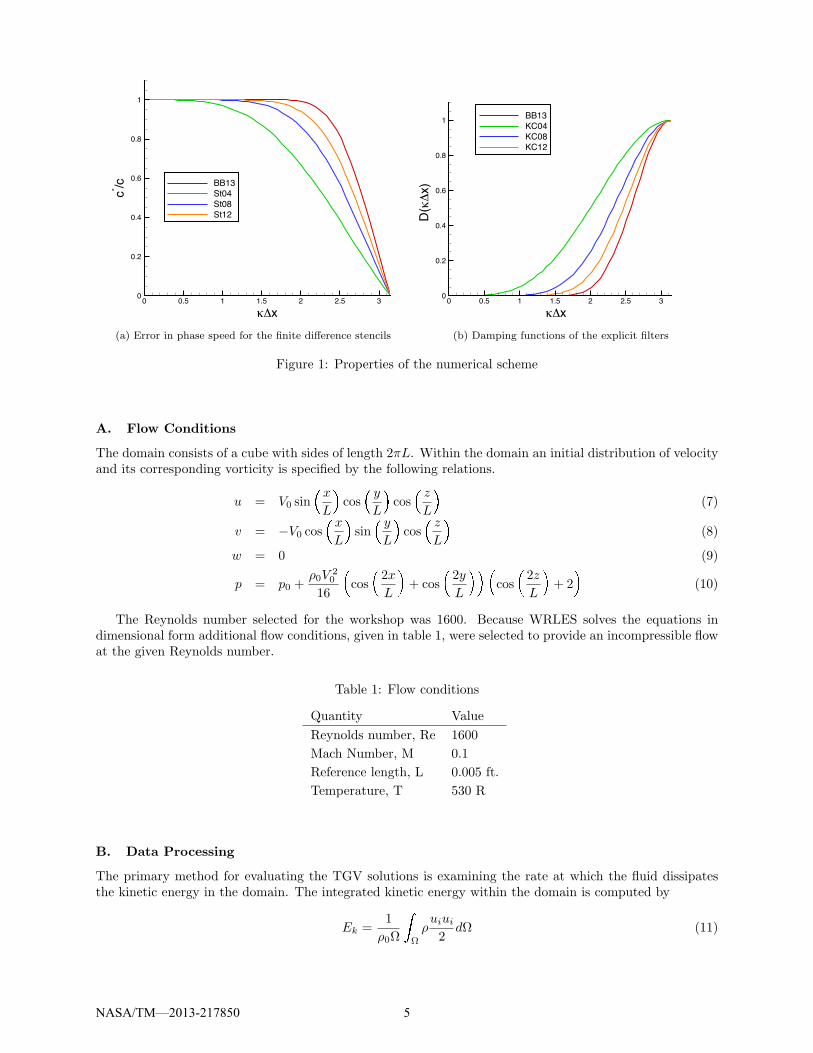
The analysis shows that central difference schemes have no inherent dissipation, and thus are ideallysuited for LES calculations. They do however produce dispersive errors. Figure 1a shows the phase error,written as the ratio of numerical phase speed to actual phase speed, c∗/c, versus normalized angular wavenumber, (κ∆x), for the schemes used in this study. For poorly resolved waves, high values of κ∆x, thescheme is unable to accurately resolve the wave.

The damping function of the filter can also be expressed in terms of κ∆x. Figure 1b shows the dampingbehavior of the KC04, KC08, KC12 and BB13 filters. The damping is minimal until it reaches a “cutoff”wave number, where it rapidly increases, effectively removing all the structures of higher waves numbers.The strength of the filter can be reduced from the default behavior by adjusting a coefficient (ranging from0 to 1) multiplying the dissipative term.

III. Problem Setup

The TGV problem can be run using a variety of flow conditions and initial conditions. The conditionsand post processing used here were specified by the organizers of the AIAA First International Workshopon High-Order Methods in Computational Fluid Dynamics.

NASA/TM—2013-217850 4

x

c*/c

0 0.5 1 1.5 2 2.5 30

0.2

0.4

0.6

0.8

1

BB13St04St08St12

(a) Error in phase speed for the finite difference stencils

x

D(

x)

0 0.5 1 1.5 2 2.5 30

0.2

0.4

0.6

0.8

1 BB13KC04KC08KC12

(b) Damping functions of the explicit filters

Figure 1: Properties of the numerical scheme

A. Flow Conditions

The domain consists of a cube with sides of length 2πL. Within the domain an initial distribution of velocityand its corresponding vorticity is specified by the following relations.

u = V0 sin x

L

cos

y

L

cos

z

L

(7)

v = −V0 cos x

L

sin

y

L

cos

z

L

(8)

w = 0 (9)

p = p0 +ρ0V

20

16

cos

2x

L

+ cos

2y

L

cos

2z

L

+ 2

(10)

The Reynolds number selected for the workshop was 1600. Because WRLES solves the equations indimensional form additional flow conditions, given in table 1, were selected to provide an incompressible flowat the given Reynolds number.

Table 1: Flow conditions

Quantity ValueReynolds number, Re 1600Mach Number, M 0.1Reference length, L 0.005 ft.Temperature, T 530 R

B. Data Processing

The primary method for evaluating the TGV solutions is examining the rate at which the fluid dissipatesthe kinetic energy in the domain. The integrated kinetic energy within the domain is computed by

Ek =1

ρ0Ω

ZΩ

ρuiui

2dΩ (11)

NASA/TM—2013-217850 5

The kinetic energy dissipation rate (KEDR) can then be computed by differencing Ek in time.

ε(Ek) = −dEk

dt(12)

This KEDR, ε, is written as a function of Ek to emphasize that it is computed directly from the kineticenergy in the domain.

A second “theoretical” kinetic energy dissipation rate can be computed from the integrated enstrophy,ζ, within the domain

ζ =1

ρ0Ω

ZΩ

ρωiωi

2dΩ (13)

It can be shown that for incompressible flow, the enstrophy is directly related to the kinetic energy dissipationrate through a constant.

ε(ζ) = 2µ

ρ0ζ (14)

The difference between the directly computed KEDR, ε(Ek), and the enstrophy based KEDR, ε(ζ), will beexamined.

Two additional quantities were computed to test the incompressible assumption. For a compressibleflow where the bulk viscosity can be taken to be zero, the “theoretical” dissipation rate is the sum of twoquantities; the contribution to the KEDR, obtained from the deviatoric strain rate tensor

ε1 = 2µ

ρ0Ω

ZΩ

SdijS

dijdΩ (15)

and the contribution to the KEDR, obtained from the pressure dilatation term.

ε3 = − 1ρ0Ω

ZΩ

p∂ui

∂xjdΩ (16)

For low Mach number flows ε3 should be negligible and the “theoretical” dissipation rate can be approximatedusing the enstrophy based KEDR (equations 13 & 14).

C. Grids

The grids were generated using a Fortran code that also computed the initial solution at t∗ = 0. The gridsare equally spaced cartesian grids of 643, 1283, 2563, and 5123 points. In order to maintain the high-orderof accuracy at the boundaries of the domain, 11 additional planes are added beyond the x = +πL, y = +πLand z = +πL boundaries and periodic conditions are enforced over a range of 6 points adjacent to theboundaries. This insures that all points within the domain are computed using the full finite differencestencil and filter stencil, and that the resolution of the scheme is maintained.

IV. Results

For the baseline and numerical scheme investigations, grid resolution studies were performed using gridsof 643, 1283, 2563, and 5123 points. For each differencing scheme and grid, the coefficient that multiplies theeffect of the filter was halved until a minimum value was found that provided a stable solution with minimaldissipation. It was found that this minimum filter coefficient was the same for all grid resolutions for a givenscheme. The nondimensional time step used for the 643 case was ∆t∗ = 3.385 · 10−3. The time step washalved for each doubling of the grid dimensions.

The 643 and 1283 cases were run on a single processor desktop workstation with six cores. The largercases were run on the NASA Pleaides high performance computing system using 8, 8-core processors forthe 2563 cases and 46, 8-core processors for the 5123 cases. Approximate wall clock time for the runs isgiven in table 2. The WRLES code was originally written for the 13-point DRP scheme. The full 13-pointstencil is always solved and there is no reduction in work for the low-order schemes. The other schemes areimplemented by changing the differencing stencil coefficients and zeroes are used where necessary for thelow-order schemes. For this reason there is no CPU time difference between schemes.

NASA/TM—2013-217850 6

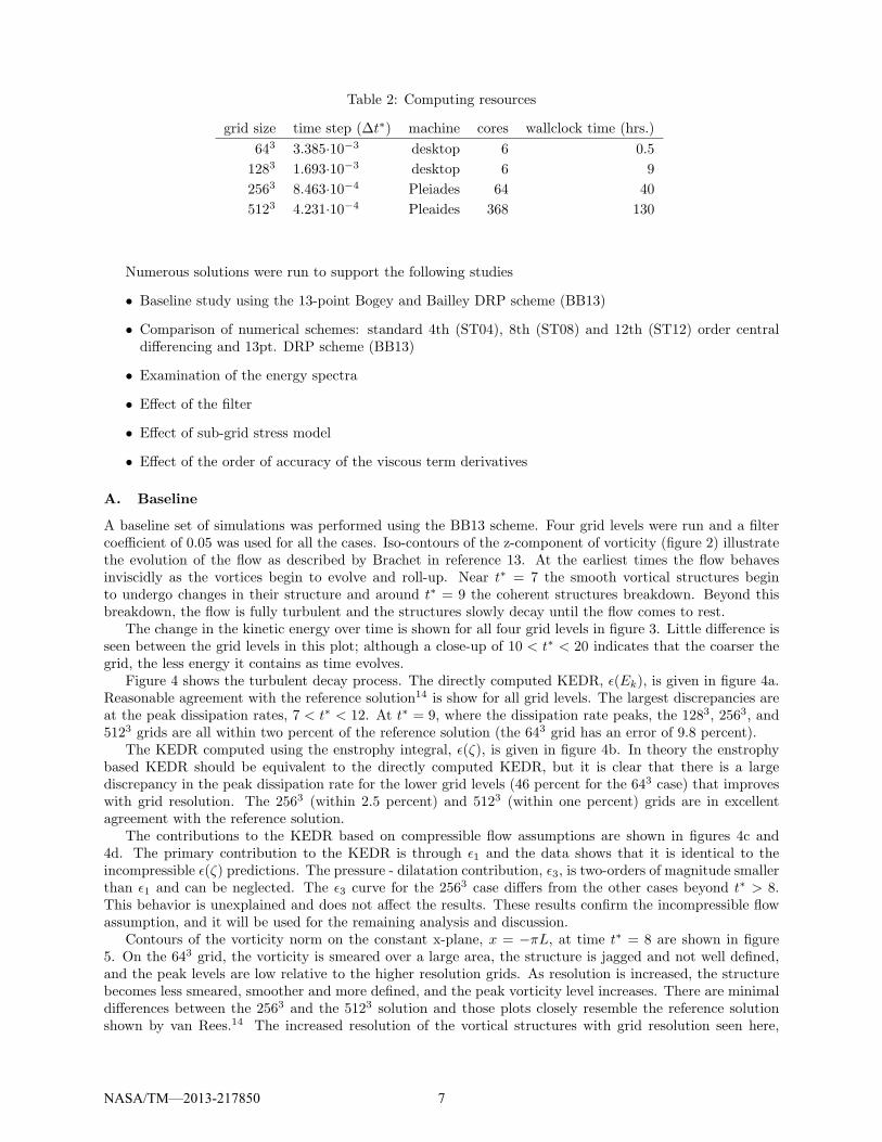
Table 2: Computing resources

grid size time step (∆t∗) machine cores wallclock time (hrs.)643 3.385·10−3 desktop 6 0.5

1283 1.693·10−3 desktop 6 92563 8.463·10−4 Pleiades 64 405123 4.231·10−4 Pleaides 368 130

Numerous solutions were run to support the following studies

• Baseline study using the 13-point Bogey and Bailley DRP scheme (BB13)

• Comparison of numerical schemes: standard 4th (ST04), 8th (ST08) and 12th (ST12) order centraldifferencing and 13pt. DRP scheme (BB13)

• Examination of the energy spectra

• Effect of the filter

• Effect of sub-grid stress model

• Effect of the order of accuracy of the viscous term derivatives

A. Baseline

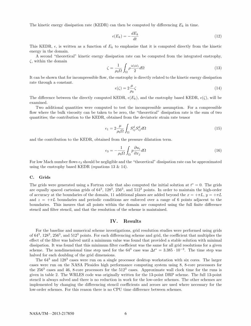
A baseline set of simulations was performed using the BB13 scheme. Four grid levels were run and a filtercoefficient of 0.05 was used for all the cases. Iso-contours of the z-component of vorticity (figure 2) illustratethe evolution of the flow as described by Brachet in reference 13. At the earliest times the flow behavesinviscidly as the vortices begin to evolve and roll-up. Near t∗ = 7 the smooth vortical structures beginto undergo changes in their structure and around t∗ = 9 the coherent structures breakdown. Beyond thisbreakdown, the flow is fully turbulent and the structures slowly decay until the flow comes to rest.

The change in the kinetic energy over time is shown for all four grid levels in figure 3. Little difference isseen between the grid levels in this plot; although a close-up of 10 < t∗ < 20 indicates that the coarser thegrid, the less energy it contains as time evolves.

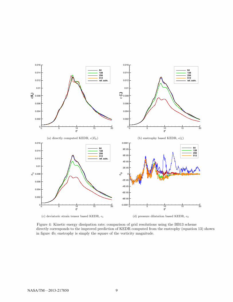
Figure 4 shows the turbulent decay process. The directly computed KEDR, ε(Ek), is given in figure 4a.Reasonable agreement with the reference solution14 is show for all grid levels. The largest discrepancies areat the peak dissipation rates, 7 < t∗ < 12. At t∗ = 9, where the dissipation rate peaks, the 1283, 2563, and5123 grids are all within two percent of the reference solution (the 643 grid has an error of 9.8 percent).

The KEDR computed using the enstrophy integral, ε(ζ), is given in figure 4b. In theory the enstrophybased KEDR should be equivalent to the directly computed KEDR, but it is clear that there is a largediscrepancy in the peak dissipation rate for the lower grid levels (46 percent for the 643 case) that improveswith grid resolution. The 2563 (within 2.5 percent) and 5123 (within one percent) grids are in excellentagreement with the reference solution.

The contributions to the KEDR based on compressible flow assumptions are shown in figures 4c and4d. The primary contribution to the KEDR is through ε1 and the data shows that it is identical to theincompressible ε(ζ) predictions. The pressure - dilatation contribution, ε3, is two-orders of magnitude smallerthan ε1 and can be neglected. The ε3 curve for the 2563 case differs from the other cases beyond t∗ > 8.This behavior is unexplained and does not affect the results. These results confirm the incompressible flowassumption, and it will be used for the remaining analysis and discussion.

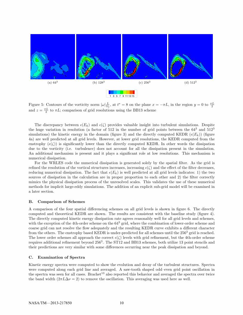
Contours of the vorticity norm on the constant x-plane, x = −πL, at time t∗ = 8 are shown in figure5. On the 643 grid, the vorticity is smeared over a large area, the structure is jagged and not well defined,and the peak levels are low relative to the higher resolution grids. As resolution is increased, the structurebecomes less smeared, smoother and more defined, and the peak vorticity level increases. There are minimaldifferences between the 2563 and the 5123 solution and those plots closely resemble the reference solutionshown by van Rees.14 The increased resolution of the vortical structures with grid resolution seen here,

NASA/TM—2013-217850 7

(a) t∗ = 3, inviscid (b) t∗ = 5, vortex roll-up (c) t∗ = 7, structure changes

(d) t∗ = 9, coherent breakdown (e) t∗ = 11, fully turbulent (f) t∗ > 11, turbulent decay

Figure 2: Iso-surfaces of z-vorticity from the BB13 scheme on the 1283 grid

t*

E k

0 5 10 15 200

0.02

0.04

0.06

0.08

0.1

0.12

0.14

64128256512ref. soln.

(a) complete simulation, 0 < t∗ < 20

t*

E k

10 12 14 16 18 200

0.02

0.04

0.06

0.08

64128256512ref. soln.

(b) close up of 10 < t∗ < 20

Figure 3: Evolution of kinetic energy

NASA/TM—2013-217850 8

t*

(Ek)

0 5 10 15 200

0.002

0.004

0.006

0.008

0.01

0.012

0.014

0.016

64128256512ref. soln.

(a) directly computed KEDR, ε(Ek)

t*

(

)

0 5 10 15 200

0.002

0.004

0.006

0.008

0.01

0.012

0.014

0.016

64128256512ref. soln.

(b) enstrophy based KEDR, ε(ζ)

t*

1

0 5 10 15 200

0.002

0.004

0.006

0.008

0.01

0.012

0.014

0.016

64128256512ref. soln.

(c) deviatoric strain tensor based KEDR, ε1

t*

3

0 5 10 15 20-0.0001

-8E-05

-6E-05

-4E-05

-2E-05

0

2E-05

4E-05

6E-05

8E-05

0.0001

64128256512

(d) pressure dilatation based KEDR, ε3

Figure 4: Kinetic energy dissipation rate; comparison of grid resolutions using the BB13 scheme

NASA/TM—2013-217850 9

directly corresponds to the improved prediction of KEDR computed from the enstrophy (equation 13) shownin figure 4b; enstrophy is simply the square of the vorticity magnitude.

(a) 643 (b) 1283 (c) 2563 (d) 5123

1 3 5 7 9 11 13 15

Figure 5: Contours of the vorticity norm |ω| LV0

, at t∗ = 8 on the plane x = −πL, in the region y = 0 to πL2

and z = πL2 to πL; comparison of grid resolutions using the BB13 scheme

The discrepancy between ε(Ek) and ε(ζ) provides valuable insight into turbulent simulations. Despitethe huge variation in resolution (a factor of 512 in the number of grid points between the 643 and 5123

simulations) the kinetic energy in the domain (figure 3) and the directly computed KEDR (ε(Ek)) (figure4a) are well predicted at all grid levels. However, at lower grid resolutions, the KEDR computed from theenstrophy (ε(ζ)) is significantly lower than the directly computed KEDR. In other words the dissipationdue to the vorticity (i.e. turbulence) does not account for all the dissipation present in the simulation.An additional mechanism is present and it plays a significant role at low resolutions. This mechanism isnumerical dissipation.

For the WRLES code the numerical dissipation is generated solely by the spatial filter. As the grid isrefined the resolution of the vortical structures increases, increasing ε(ζ) and the effect of the filter decreases,reducing numerical dissipation. The fact that ε(Ek) is well predicted at all grid levels indicates: 1) the twosources of dissipation in the calculation are in proper proportion to each other and 2) the filter correctlymimics the physical dissipation process of the unresolved scales. This validates the use of these numericalmethods for implicit large-eddy simulations. The addition of an explicit sub-grid model will be examined ina later section.

B. Comparison of Schemes

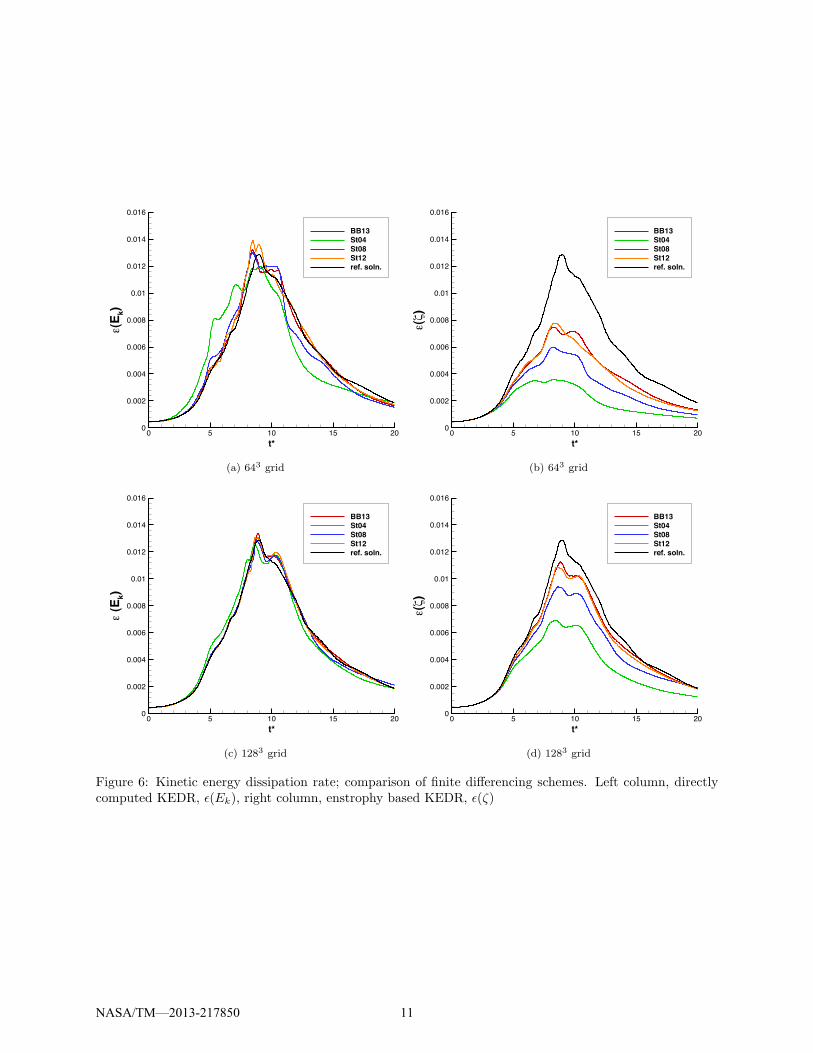
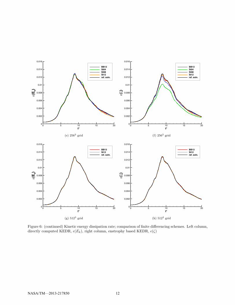
A comparison of the four spatial differencing schemes on all grid levels is shown in figure 6. The directlycomputed and theoretical KEDR are shown. The results are consistent with the baseline study (figure 4).The directly computed kinetic energy dissipation rate agrees reasonably well for all grid levels and schemes,with the exception of the 4th-order scheme on the 643 grid, where the combination of lower-order scheme andcoarse grid can not resolve the flow adequately and the resulting KEDR curve exhibits a different characterfrom the others. The enstrophy based KEDR is under-predicted for all schemes until the 2563 grid is reached.The lower order schemes all approach the correct ε(ζ) levels with grid refinement, but the 4th-order schemerequires additional refinement beyond 2563. The ST12 and BB13 schemes, both utilize 13 point stencils andtheir predictions are very similar with some differences occurring near the peak dissipation and beyond.

C. Examination of Spectra

Kinetic energy spectra were computed to show the evolution and decay of the turbulent structures. Spectrawere computed along each grid line and averaged. A saw-tooth shaped odd–even grid point oscillation inthe spectra was seen for all cases. Brachet13 also reported this behavior and averaged the spectra over twicethe band width (2πL∆ν = 2) to remove the oscillation. This averaging was used here as well.

NASA/TM—2013-217850 10

t*

(Ek)

0 5 10 15 200

0.002

0.004

0.006

0.008

0.01

0.012

0.014

0.016

BB13St04St08St12ref. soln.

(a) 643 grid

t*

()

0 5 10 15 200

0.002

0.004

0.006

0.008

0.01

0.012

0.014

0.016

BB13St04St08St12ref. soln.

(b) 643 grid

t*

(Ek)

0 5 10 15 200

0.002

0.004

0.006

0.008

0.01

0.012

0.014

0.016

BB13St04St08St12ref. soln.

(c) 1283 grid

t*

()

0 5 10 15 200

0.002

0.004

0.006

0.008

0.01

0.012

0.014

0.016

BB13St04St08St12ref. soln.

(d) 1283 grid

Figure 6: Kinetic energy dissipation rate; comparison of finite differencing schemes. Left column, directlycomputed KEDR, ε(Ek), right column, enstrophy based KEDR, ε(ζ)

NASA/TM—2013-217850 11

t*

(Ek)

0 5 10 15 200

0.002

0.004

0.006

0.008

0.01

0.012

0.014

0.016

BB13St04St08St12ref. soln.

(e) 2563 grid

t*

()

0 5 10 15 200

0.002

0.004

0.006

0.008

0.01

0.012

0.014

0.016

BB13St04St08St12ref. soln.

(f) 2563 grid

t*

(Ek)

0 5 10 15 200

0.002

0.004

0.006

0.008

0.01

0.012

0.014

0.016

BB13St12ref. soln.

(g) 5123 grid

t*

()

0 5 10 15 200

0.002

0.004

0.006

0.008

0.01

0.012

0.014

0.016

BB13St12ref. soln.

(h) 5123 grid

Figure 6: (continued) Kinetic energy dissipation rate; comparison of finite differencing schemes. Left column,directly computed KEDR, ε(Ek), right column, enstrophy based KEDR, ε(ζ)

NASA/TM—2013-217850 12

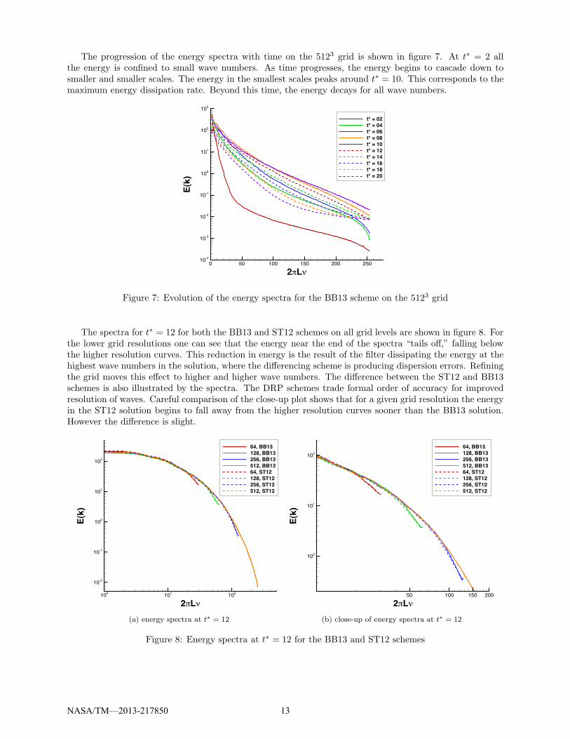
The progression of the energy spectra with time on the 5123 grid is shown in figure 7. At t∗ = 2 allthe energy is confined to small wave numbers. As time progresses, the energy begins to cascade down tosmaller and smaller scales. The energy in the smallest scales peaks around t∗ = 10. This corresponds to themaximum energy dissipation rate. Beyond this time, the energy decays for all wave numbers.

2 L

E(k)

0 50 100 150 200 25010-4

10-3

10-2

10-1

100

101

102

103

t* = 02t* = 04t* = 06t* = 08t* = 10t* = 12t* = 14t* = 16t* = 18t* = 20

Figure 7: Evolution of the energy spectra for the BB13 scheme on the 5123 grid

The spectra for t∗ = 12 for both the BB13 and ST12 schemes on all grid levels are shown in figure 8. Forthe lower grid resolutions one can see that the energy near the end of the spectra “tails off,” falling belowthe higher resolution curves. This reduction in energy is the result of the filter dissipating the energy at thehighest wave numbers in the solution, where the differencing scheme is producing dispersion errors. Refiningthe grid moves this effect to higher and higher wave numbers. The difference between the ST12 and BB13schemes is also illustrated by the spectra. The DRP schemes trade formal order of accuracy for improvedresolution of waves. Careful comparison of the close-up plot shows that for a given grid resolution the energyin the ST12 solution begins to fall away from the higher resolution curves sooner than the BB13 solution.However the difference is slight.

2 L

E(k)

100 101 102

10-2

10-1

100

101

102

64, BB13128, BB13256, BB13512, BB1364, ST12128, ST12256, ST12512, ST12

(a) energy spectra at t∗ = 12

2 L

E(k)

50 100 150 200

100

101

10264, BB13128, BB13256, BB13512, BB1364, ST12128, ST12256, ST12512, ST12

(b) close-up of energy spectra at t∗ = 12

Figure 8: Energy spectra at t∗ = 12 for the BB13 and ST12 schemes

NASA/TM—2013-217850 13

D. Effect of the Filter

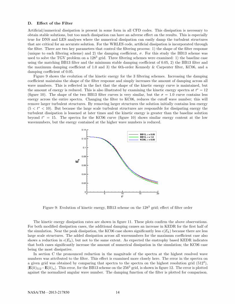
Artificial/numerical dissipation is present in some form in all CFD codes. This dissipation is necessary toobtain stable solutions, but too much dissipation can have an adverse effect on the results. This is especiallytrue for DNS and LES analyses where the numerical dissipation can easily damp the turbulent structuresthat are critical for an accurate solution. For the WRLES code, artificial dissipation is incorporated throughthe filter. There are two key parameters that control the filtering process: 1) the shape of the filter response(unique to each filtering scheme) and 2) the damping coefficient, σ. For this study the BB13 scheme wasused to solve the TGV problem on a 1283 grid. Three filtering schemes were examined: 1) the baseline caseusing the matching BB13 filter and the minimum stable damping coefficient of 0.05, 2) the BB13 filter andthe maximum damping coefficient of 1.0 and 3) the 6th-order Kennedy & Carpenter filter, KC06, and adamping coefficient of 0.05.

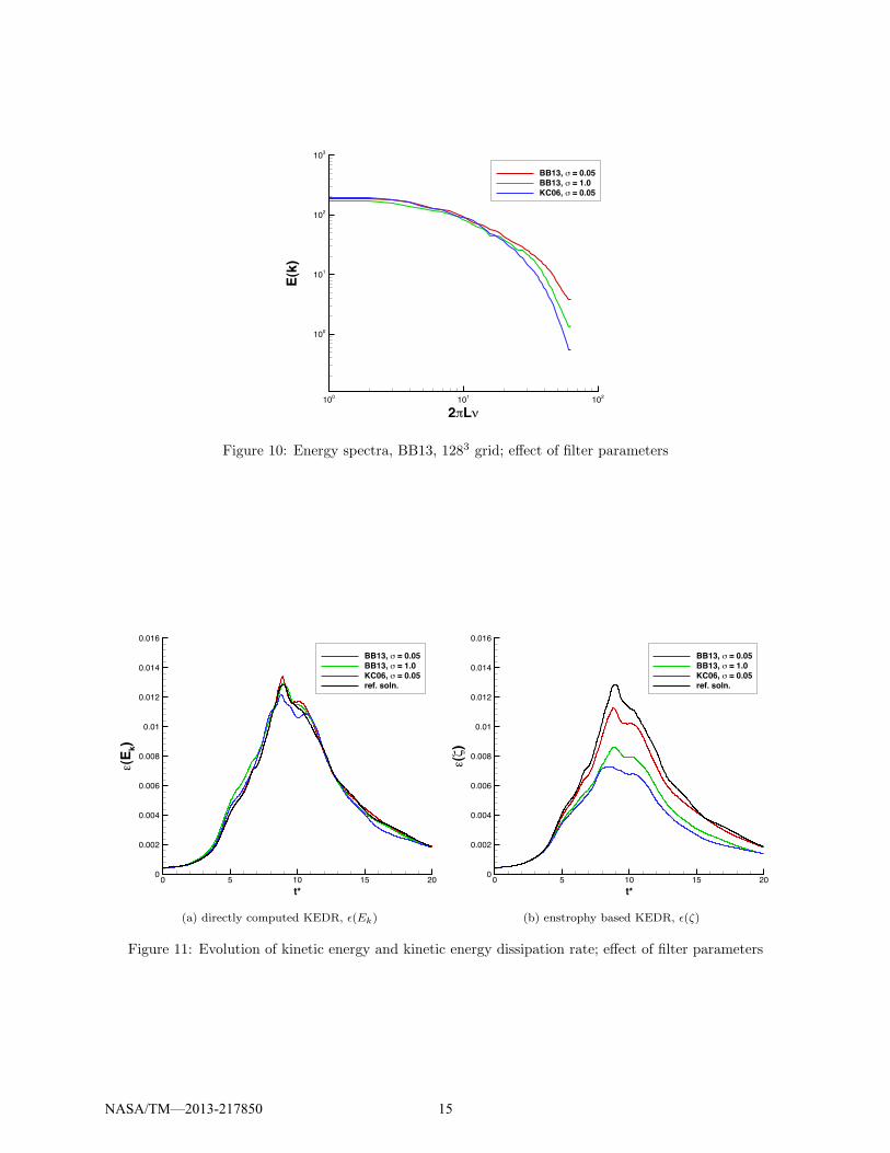
Figure 9 shows the evolution of the kinetic energy for the 3 filtering schemes. Increasing the dampingcoefficient maintains the shape of the filter response and simply increases the amount of damping across allwave numbers. This is reflected in the fact that the shape of the kinetic energy curve is maintained, butthe amount of energy is reduced. This is also illustrated by examining the kinetic energy spectra at t∗ = 12(figure 10). The shape of the two BB13 filter curves is very similar, but the σ = 1.0 curve contains lessenergy across the entire spectra. Changing the filter to KC06, reduces the cutoff wave number; this willremove larger turbulent structures. By removing larger structures the solution initially contains less energy(5 < t∗ < 10). But because the large scale turbulent structures are responsible for dissipating energy theturbulent dissipation is lessened at later times and the kinetic energy is greater than the baseline solutionbeyond t∗ = 15. The spectra for the KC06 curve (figure 10) shows similar energy content at the lowwavenumbers, but the energy contained at the higher wave numbers is reduced.

t*

E k

0 5 10 15 200

0.02

0.04

0.06

0.08

0.1

0.12

0.14

BB13, = 0.05BB13, = 1.0KC06, = 0.05

Figure 9: Evolution of kinetic energy, BB13 scheme on the 1283 grid; effect of filter order

The kinetic energy dissipation rates are shown in figure 11. These plots confirm the above observations.For both modified dissipation cases, the additional damping causes an increase in KEDR for the first half ofthe simulation. Near the peak dissipation, the KC06 case shows significantly less ε(Ek) because there are lesslarge scale structures. The added dissipation across all wavenumbers for the maximum coefficient case alsoshows a reduction in ε(Ek), but not to the same extent. As expected the enstrophy based KEDR indicatesthat both cases significantly increase the amount of numerical dissipation in the simulation; the KC06 casebeing the most dissipative.

In section C the pronounced reduction in the magnitude of the spectra at the highest resolved wavenumbers was attributed to the filter. This effect is examined more closely here. The error in the spectra ona given grid was obtained by comparing that spectra to the spectra on the highest resolution grid (5123),|E(k)512−E(k)n|. This error, for the BB13 scheme on the 2563 grid, is shown in figure 12. The error is plottedagainst the normalized angular wave number. The damping function of the filter is plotted for comparison.

NASA/TM—2013-217850 14

2 L

E(k)

100 101 102

100

101

102

103

BB13, = 0.05BB13, = 1.0KC06, = 0.05

Figure 10: Energy spectra, BB13, 1283 grid; effect of filter parameters

t*

(Ek)

0 5 10 15 200

0.002

0.004

0.006

0.008

0.01

0.012

0.014

0.016

BB13, = 0.05BB13, = 1.0KC06, = 0.05ref. soln.

(a) directly computed KEDR, ε(Ek)

t*

()

0 5 10 15 200

0.002

0.004

0.006

0.008

0.01

0.012

0.014

0.016

BB13, = 0.05BB13, = 1.0KC06, = 0.05ref. soln.

(b) enstrophy based KEDR, ε(ζ)

Figure 11: Evolution of kinetic energy and kinetic energy dissipation rate; effect of filter parameters

NASA/TM—2013-217850 15

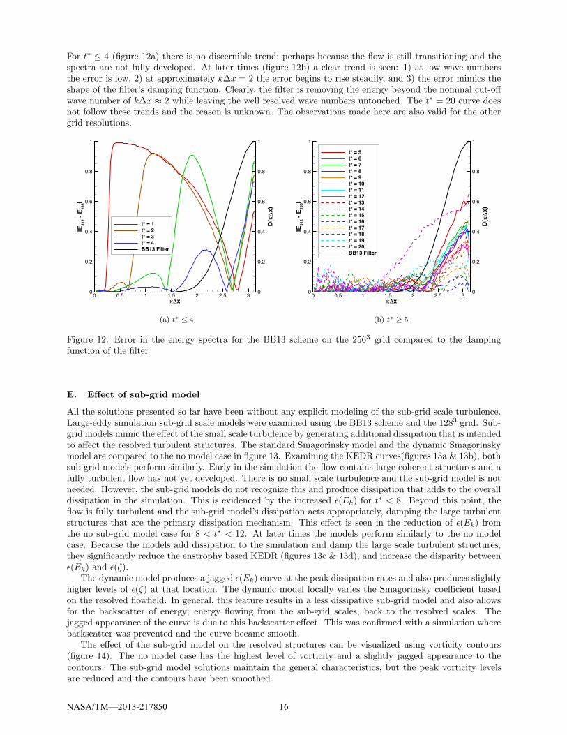
For t∗ ≤ 4 (figure 12a) there is no discernible trend; perhaps because the flow is still transitioning and thespectra are not fully developed. At later times (figure 12b) a clear trend is seen: 1) at low wave numbersthe error is low, 2) at approximately k∆x = 2 the error begins to rise steadily, and 3) the error mimics theshape of the filter’s damping function. Clearly, the filter is removing the energy beyond the nominal cut-offwave number of k∆x ≈ 2 while leaving the well resolved wave numbers untouched. The t∗ = 20 curve doesnot follow these trends and the reason is unknown. The observations made here are also valid for the othergrid resolutions.

x

|E51

2 - E

256|

D(

x)

0 0.5 1 1.5 2 2.5 30

0.2

0.4

0.6

0.8

1

0

0.2

0.4

0.6

0.8

1

t* = 1t* = 2t* = 3t* = 4BB13 Filter

(a) t∗ ≤ 4

x|E

512 -

E25

6|

D(

x)

0 0.5 1 1.5 2 2.5 30

0.2

0.4

0.6

0.8

1

0

0.2

0.4

0.6

0.8

1

t* = 5t* = 6t* = 7t* = 8t* = 9t* = 10t* = 11t* = 12t* = 13t* = 14t* = 15t* = 16t* = 17t* = 18t* = 19t* = 20BB13 Filter

(b) t∗ ≥ 5

Figure 12: Error in the energy spectra for the BB13 scheme on the 2563 grid compared to the dampingfunction of the filter

E. Effect of sub-grid model

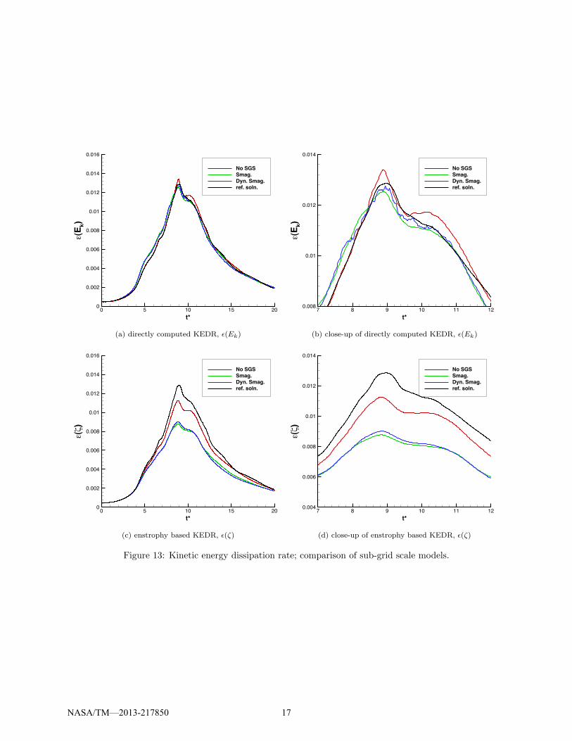
All the solutions presented so far have been without any explicit modeling of the sub-grid scale turbulence.Large-eddy simulation sub-grid scale models were examined using the BB13 scheme and the 1283 grid. Sub-grid models mimic the effect of the small scale turbulence by generating additional dissipation that is intendedto affect the resolved turbulent structures. The standard Smagorinsky model and the dynamic Smagorinskymodel are compared to the no model case in figure 13. Examining the KEDR curves(figures 13a & 13b), bothsub-grid models perform similarly. Early in the simulation the flow contains large coherent structures and afully turbulent flow has not yet developed. There is no small scale turbulence and the sub-grid model is notneeded. However, the sub-grid models do not recognize this and produce dissipation that adds to the overalldissipation in the simulation. This is evidenced by the increased ε(Ek) for t∗ < 8. Beyond this point, theflow is fully turbulent and the sub-grid model’s dissipation acts appropriately, damping the large turbulentstructures that are the primary dissipation mechanism. This effect is seen in the reduction of ε(Ek) fromthe no sub-grid model case for 8 < t∗ < 12. At later times the models perform similarly to the no modelcase. Because the models add dissipation to the simulation and damp the large scale turbulent structures,they significantly reduce the enstrophy based KEDR (figures 13c & 13d), and increase the disparity betweenε(Ek) and ε(ζ).

The dynamic model produces a jagged ε(Ek) curve at the peak dissipation rates and also produces slightlyhigher levels of ε(ζ) at that location. The dynamic model locally varies the Smagorinsky coefficient basedon the resolved flowfield. In general, this feature results in a less dissipative sub-grid model and also allowsfor the backscatter of energy; energy flowing from the sub-grid scales, back to the resolved scales. Thejagged appearance of the curve is due to this backscatter effect. This was confirmed with a simulation wherebackscatter was prevented and the curve became smooth.

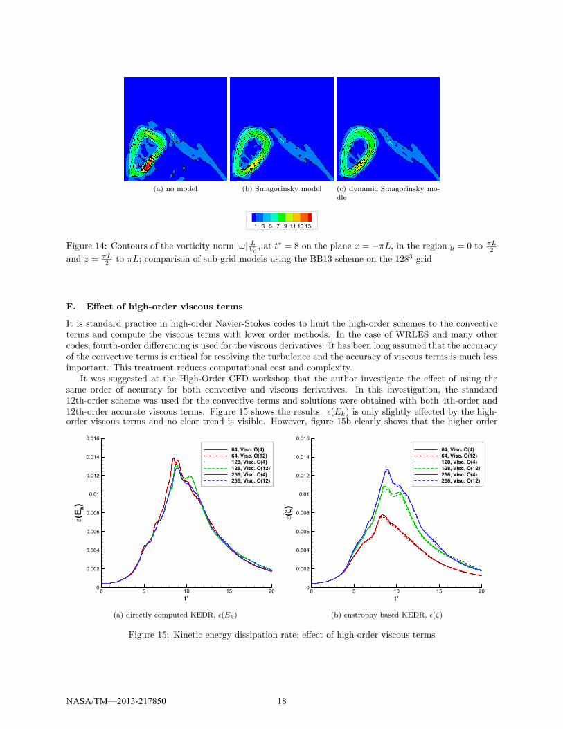
The effect of the sub-grid model on the resolved structures can be visualized using vorticity contours(figure 14). The no model case has the highest level of vorticity and a slightly jagged appearance to the

NASA/TM—2013-217850 16

contours. The sub-grid model solutions maintain the general characteristics, but the peak vorticity levelsare reduced and the contours have been smoothed.

t*

(Ek)

0 5 10 15 200

0.002

0.004

0.006

0.008

0.01

0.012

0.014

0.016

No SGSSmag.Dyn. Smag.ref. soln.

(a) directly computed KEDR, ε(Ek)

t*

(Ek)

7 8 9 10 11 120.008

0.01

0.012

0.014

No SGSSmag.Dyn. Smag.ref. soln.

(b) close-up of directly computed KEDR, ε(Ek)

t*

()

0 5 10 15 200

0.002

0.004

0.006

0.008

0.01

0.012

0.014

0.016

No SGSSmag.Dyn. Smag.ref. soln.

(c) enstrophy based KEDR, ε(ζ)

t*

()

7 8 9 10 11 120.004

0.006

0.008

0.01

0.012

0.014

No SGSSmag.Dyn. Smag.ref. soln.

(d) close-up of enstrophy based KEDR, ε(ζ)

Figure 13: Kinetic energy dissipation rate; comparison of sub-grid scale models.

NASA/TM—2013-217850 17

(a) no model (b) Smagorinsky model (c) dynamic Smagorinsky mo-dle

1 3 5 7 9 11 13 15

Figure 14: Contours of the vorticity norm |ω| LV0

, at t∗ = 8 on the plane x = −πL, in the region y = 0 to πL2

and z = πL2 to πL; comparison of sub-grid models using the BB13 scheme on the 1283 grid

F. Effect of high-order viscous terms

It is standard practice in high-order Navier-Stokes codes to limit the high-order schemes to the convectiveterms and compute the viscous terms with lower order methods. In the case of WRLES and many othercodes, fourth-order differencing is used for the viscous derivatives. It has been long assumed that the accuracyof the convective terms is critical for resolving the turbulence and the accuracy of viscous terms is much lessimportant. This treatment reduces computational cost and complexity.

It was suggested at the High-Order CFD workshop that the author investigate the effect of using thesame order of accuracy for both convective and viscous derivatives. In this investigation, the standard12th-order scheme was used for the convective terms and solutions were obtained with both 4th-order and12th-order accurate viscous terms. Figure 15 shows the results. ε(Ek) is only slightly effected by the high-

t*

(Ek)

0 5 10 15 200

0.002

0.004

0.006

0.008

0.01

0.012

0.014

0.016

64, Visc. O(4)64, Visc. O(12)128, Visc. O(4)128, Visc. O(12)256, Visc. O(4)256, Visc. O(12)

(a) directly computed KEDR, ε(Ek)

t*

()

0 5 10 15 200

0.002

0.004

0.006

0.008

0.01

0.012

0.014

0.016

64, Visc. O(4)64, Visc. O(12)128, Visc. O(4)128, Visc. O(12)256, Visc. O(4)256, Visc. O(12)

(b) enstrophy based KEDR, ε(ζ)

Figure 15: Kinetic energy dissipation rate; effect of high-order viscous terms

order viscous terms and no clear trend is visible. However, figure 15b clearly shows that the higher order

NASA/TM—2013-217850 18

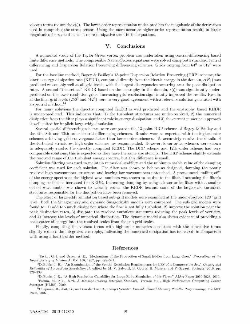
viscous terms reduce the ε(ζ). The lower-order representation under-predicts the magnitude of the derivativesused in computing the stress tensor. Using the more accurate higher-order representation results in largermagnitudes for τij and hence a more dissipative term in the equations.

V. Conclusions

A numerical study of the Taylor-Green vortex problem was undertaken using central-differencing basedfinite difference methods. The compressible Navier-Stokes equations were solved using both standard centraldifferencing and Dispersion Relation Preserving differencing schemes. Grids ranging from 643 to 5123 wereused.

For the baseline method, Bogey & Bailley’s 13-point Dispersion Relation Preserving (DRP) scheme, thekinetic energy dissipation rate (KEDR), computed directly from the kinetic energy in the domain, ε(Ek) waspredicted reasonably well at all grid levels, with the largest discrepancies occurring near the peak dissipationrates. A second “theoretical” KEDR based on the enstrophy in the domain, ε(ζ) was significantly under-predicted on the lower resolution grids. Increasing grid resolution significantly improved the results. Resultsat the finer grid levels (2563 and 5123) were in very good agreement with a reference solution generated witha spectral method.14

For many solutions the directly computed KEDR is well predicted and the enstrophy based KEDRis under-predicted. This indicates that: 1) the turbulent structures are under-resolved, 2) the numericaldissipation from the filter plays a significant role in energy dissipation, and 3) the current numerical approachis well suited for implicit large-eddy simulation.

Several spatial differencing schemes were compared: the 13-point DRP scheme of Bogey & Bailley andthe 4th, 8th and 12th order central differencing schemes. Results were as expected with the higher-orderschemes achieving grid convergence faster than lower-order schemes. To accurately resolve the details ofthe turbulent structures, high-order schemes are recommended. However, lower-order schemes were shownto adequately resolve the directly computed KEDR. The DRP scheme and 12th order scheme had verycomparable solutions; this is expected as they have the same size stencils. The DRP scheme slightly extendsthe resolved range of the turbulent energy spectra, but this difference is small.

Solution filtering was used to maintain numerical stability and the minimum stable value of the dampingcoefficient was used for each solution. The filter was shown to behave as designed, damping the poorlyresolved high wavenumber structures and leaving low wavenumbers untouched. A pronounced “tailing off”of the energy spectra at the highest wave numbers was shown to be due to the filter. Increasing the filter’sdamping coefficient increased the KEDR. Increasing damping by using a lower-order filter with a smallercut-off wavenumber was shown to actually reduce the KEDR because some of the large-scale turbulentstructures responsible for the dissipation have been removed.

The effect of large-eddy simulation based sub-grid models were examined at the under-resolved 1283 gridlevel. Both the Smagorinsky and dynamic Smagorinsky models were compared. The sub-grid models werefound to: 1) add too much dissipation where the flow is not fully turbulent, 2) improve the solution near thepeak dissipation rates, 3) dissipate the resolved turbulent structures reducing the peak levels of vorticity,and 4) increase the levels of numerical dissipation. The dynamic model also shows evidence of providing abackscatter of energy into the resolved scales from the sub-grid scales.

Finally, computing the viscous terms with high-order numerics consistent with the convective termsslightly reduces the integrated enstrophy, indicating the numerical dissipation has increased, in comparisonwith using a fourth-order method.

References

1Taylor, G. I. and Green, A. E., “Mechanisms of the Production of Small Eddies from Large Ones,” Proceedings of theRoyal Society of London A, Vol. 158, 1937, pp. 499–521.

2DeBonis, J. R., “An Examination of the Spatial Resolution Requirements for LES of a Compressible Jet,” Quality andReliability of Large-Eddy Simulation II , edited by M. V. Salvetti, B. Geurts, H. Meyers, and P. Sagaut, Springer, 2010, pp.329–338.

3DeBonis, J. R., “A High-Resolution Capability for Large-Eddy Simulation of Jet Flows,” AIAA Paper 2010-5023, 2010.4Forum, M. P. I., MPI: A Message-Passing Interface Standard, Version 2.2 , High Performance Computing Center

Stuttgart (HLRS), 2009.5Chapman, B., Jost, G., and van der Pas, R., Using OpenMP: Portable Shared Memory Parallel Programming, The MIT

Press, 2007.

NASA/TM—2013-217850 19

6Smagorinsky, J., “General Circulation Experiments with the Primitive Equations, Part I: The Basic Experiment,” MonthlyWeather Review , Vol. 91, 1963, pp. 99–152.

7Lilly, D. K., “A Proposed Modification of the Germano Subgrid-Scale Closure Method,” Physics of Fluids A, Vol. 4,No. 3, 1992, pp. 633–635.

8Williamson, J. H., “Low-Storage Runge-Kutta Schemes,” Journal of Computational Physics, Vol. 35, 1980, pp. 48.9Carpenter, M. H. and Kennedy, C. A., “Fourth-Order 2N-Storage Runge-Kutta Schemes,” NASA TM 109112, 1994.

10Bogey, C. and Bailly, C., “A Family of Low Dispersive and Low Dissipative Explicit Schemes for Flow and NoiseComputations,” Journal of Computational Physics, Vol. 194, 2004, pp. 194–214.

11Kennedy, C. A. and Carpenter, M. H., “Comparison of Several Numerical Methods for Simulation of Compressible ShearLayers,” NASA TP 3484, 1997.

12Vichnevetsky, R. and Bowles, J. B., Fourier Analysis of Numerical Approximations of Hyperbolic Equations, Society forApplied and Industrial Mathematics, 1982.

13Brachet, M. E., Meiron, D. I., Orszag, S. A., Nickel, B. G., Morf, R. H., and Frisch, U., “Small-scale structure of theTaylor-Green Vortex,” Journal of Fluid Mechanics, Vol. 130, 1983, pp. 411–452.

14van Rees, W. M., Leonard, A., Pullin, D. I., and Koumoutsakos, P., “A Comparison of Vortex and Pseudo-SpectralMethods for the Simulation of Periodic Vortical Flows at High Reynolds Numbers,” Journal of Computational Physics, Vol. 230,2011, pp. 2794–2805.

NASA/TM—2013-217850 20

REPORT DOCUMENTATION PAGE Form Approved OMB No. 0704-0188

The public reporting burden for this collection of information is estimated to average 1 hour per response, including the time for reviewing instructions, searching existing data sources, gathering and maintaining the data needed, and completing and reviewing the collection of information. Send comments regarding this burden estimate or any other aspect of this collection of information, including suggestions for reducing this burden, to Department of Defense, Washington Headquarters Services, Directorate for Information Operations and Reports (0704-0188), 1215 Jefferson Davis Highway, Suite 1204, Arlington, VA 22202-4302. Respondents should be aware that notwithstanding any other provision of law, no person shall be subject to any penalty for failing to comply with a collection of information if it does not display a currently valid OMB control number. PLEASE DO NOT RETURN YOUR FORM TO THE ABOVE ADDRESS.

1. REPORT DATE (DD-MM-YYYY) 01-02-2013

2. REPORT TYPE Technical Memorandum

3. DATES COVERED (From - To)

4. TITLE AND SUBTITLE Solutions of the Taylor-Green Vortex Problem Using High-Resolution Explicit Finite Difference Methods

5a. CONTRACT NUMBER

5b. GRANT NUMBER

5c. PROGRAM ELEMENT NUMBER

6. AUTHOR(S) DeBonis, James, R.

5d. PROJECT NUMBER

5e. TASK NUMBER

5f. WORK UNIT NUMBER WBS 561581.02.08.03.48.01

7. PERFORMING ORGANIZATION NAME(S) AND ADDRESS(ES) National Aeronautics and Space Administration John H. Glenn Research Center at Lewis Field Cleveland, Ohio 44135-3191

8. PERFORMING ORGANIZATION REPORT NUMBER E-18637

9. SPONSORING/MONITORING AGENCY NAME(S) AND ADDRESS(ES) National Aeronautics and Space Administration Washington, DC 20546-0001

10. SPONSORING/MONITOR'S ACRONYM(S) NASA

11. SPONSORING/MONITORING REPORT NUMBER NASA/TM-2013-217850

12. DISTRIBUTION/AVAILABILITY STATEMENT Unclassified-Unlimited Subject Categories: 34 and 02 Available electronically at http://www.sti.nasa.gov This publication is available from the NASA Center for AeroSpace Information, 443-757-5802

13. SUPPLEMENTARY NOTES

14. ABSTRACT A computational fluid dynamics code that solves the compressible Navier-Stokes equations was applied to the Taylor-Green vortex problem to examine the code’s ability to accurately simulate the vortex decay and subsequent turbulence. The code, WRLES (Wave Resolving Large-Eddy Simulation), uses explicit central-differencing to compute the spatial derivatives and explicit Low Dispersion Runge-Kutta methods for the temporal discretization. The flow was first studied and characterized using Bogey & Bailley’s 13-point dispersion relation preserving (DRP) scheme. The kinetic energy dissipation rate, computed both directly and from the enstrophy field, vorticity contours, and the energy spectra are examined. Results are in excellent agreement with a reference solution obtained using a spectral method and provide insight into computations of turbulent flows. In addition the following studies were performed: a comparison of 4th-, 8th-, 12th- and DRP spatial differencing schemes, the effect of the solution filtering on the results, the effect of large-eddy simulation sub-grid scale models, and the effect of high-order discretization of the viscous terms.15. SUBJECT TERMS Turbulence; Computational fluid dynamics; Vorticity; Large-eddy simulation; Direct numerical simulation

16. SECURITY CLASSIFICATION OF: 17. LIMITATION OF ABSTRACT UU

18. NUMBER OF PAGES

28

19a. NAME OF RESPONSIBLE PERSON STI Help Desk (email:help@sti.nasa.gov)

a. REPORT U

b. ABSTRACT U

c. THIS PAGE U

19b. TELEPHONE NUMBER (include area code) 443-757-5802

Standard Form 298 (Rev. 8-98)Prescribed by ANSI Std. Z39-18