SOLUTIONS OF LARGE-SCALE ELECTROMAGNETICS PROBLEMS USING ... · Progress In Electromagnetics Research, Vol. 106, 203{223, 2010 SOLUTIONS OF LARGE-SCALE ELECTROMAGNETICS PROBLEMS USING

Progress In Electromagnetics Research, Vol. 106, 203–223, 2010

SOLUTIONS OF LARGE-SCALE ELECTROMAGNETICSPROBLEMS USING AN ITERATIVE INNER-OUTERSCHEME WITH ORDINARY AND APPROXIMATEMULTILEVEL FAST MULTIPOLE ALGORITHMS

O. Ergul, T. Malas, and L. Gurel †

Computational Electromagnetics Research Center (BiLCEM)Bilkent UniversityAnkara, Turkey

Abstract—We present an iterative inner-outer scheme for the efficientsolution of large-scale electromagnetics problems involving perfectly-conducting objects formulated with surface integral equations.Problems are solved by employing the multilevel fast multipolealgorithm (MLFMA) on parallel computer systems. In orderto construct a robust preconditioner, we develop an approximateMLFMA (AMLFMA) by systematically increasing the efficiency ofthe ordinary MLFMA. Using a flexible outer solver, iterative MLFMAsolutions are accelerated via an inner iterative solver, employingAMLFMA and serving as a preconditioner to the outer solver.The resulting implementation is tested on various electromagneticsproblems involving both open and closed conductors. We show thatthe processing time decreases significantly using the proposed method,compared to the solutions obtained with conventional preconditionersin the literature.

1. INTRODUCTION

For numerical solutions of electromagnetics problems involving metallic(conducting) objects, simultaneous discretizations of surfaces and theintegral-equation formulations lead to N ×N dense matrix equations,

Received 17 June 2010, Accepted 2 July 2010, Scheduled 22 July 2010

Corresponding author: O. Ergul ([email protected]).† O. Ergul is now with the Department of Mathematics and Statistics, University ofStrathclyde, Glasgow, UK; T. Malas is now with the Department of Electrical andComputer Engineering, The University of Texas at Austin, Austin, Texas; L. Gurel isalso with the Department of Electrical and Electronics Engineering, Bilkent University,Ankara, Turkey.

204 Ergul, Malas, and Gurel

which can be solved iteratively by using a Krylov subspace algorithm.On the other hand, most of the real-life applications involve largegeometries that need to be discretized with millions of unknowns. Forsuch large-scale problems, it is necessary to reduce the complexityof the matrix-vector multiplications required by an iterative solver.The required acceleration is provided by the multilevel fast multipolealgorithm (MLFMA), which is based on calculating the interactionsbetween the discretization elements in a group-by-group manner [1].This is achieved by applying the addition theorem to factorize the free-space Green’s function and performing a diagonalization to expand thespherical wave functions in a series of plane waves [2]. Constructinga tree structure of clusters‡ by recursively dividing a computationalbox enclosing the object, MLFMA computes the interactions in amultilevel scheme and reduces the processing time of a dense matrix-vector multiplication from O(N2) to O(N log N). In addition, only asparse part of the full matrix, namely, the near-field matrix, needs to bestored so that the memory requirement is also reduced to O(N log N).Consequently, MLFMA renders the solution of large matrix equationspossible on relatively inexpensive computing platforms.

MLFMA offers remarkable advantages for the iterative solutionof integral-equation formulations by reducing the complexity of thematrix-vector multiplications [3, 4]. However, particularly for large-scale problems, it is desirable to further reduce the total cost of theiterative solutions. For example, Bouras and Fraysse [5] proposeddecreasing the accuracy of the matrix-vector multiplications in thejth iteration by relating the relative error δj of the matrix-vectormultiplication to the norm of the residual vector ρj , i.e.,

δj =

ε, ‖ρj‖2 > 1ε

‖ρj‖2, ε ≤ ‖ρj‖2 ≤ 1

1, ‖ρj‖2 < ε,

(1)

where ε ≤ 1 denotes the target residual error. Using (1), the relativeerror of the matrix-vector multiplication is relaxed from ε to 1 as theiterations proceed. However, using a similar relaxation strategy byadjusting the accuracy of MLFMA during the course of an iterativesolution is not trivial. This is because the implementation details ofMLFMA depend on the targeted accuracy. In principle, it is possibleto construct a fixed number of MLFMA versions with various levelsof accuracy. Nevertheless, each version increases the cost of thesetup substantially. Moreover, a less-accurate MLFMA obtained by‡ Throughout this paper, the term “clusters” is used to indicate “boxes” and “sub-boxes”in an MLFMA oct-tree.

Progress In Electromagnetics Research, Vol. 106, 2010 205

decreasing the number of accurate digits is not significantly cheaperthan the ordinary MLFMA.

Another option for reducing the cost of an iterative solutionis to use preconditioners to accelerate the iterative convergence.In MLFMA, the sparse near-field matrix is available to constructeffective preconditioners for relatively small problems. However, as theproblem size grows, sparsity of the near-field matrix increases, and theresulting preconditioners become insufficient to accelerate the iterativeconvergence.

In this paper, we present efficient solutions of large-scaleelectromagnetics problems using ordinary and approximate versionsof MLFMA in an inner-outer scheme [6, 7]. Outer iterativesolutions are performed by using a flexible solver accelerated by anordinary MLFMA. Those solutions are effectively preconditioned byanother Krylov-subspace algorithm accelerated by an approximateMLFMA (AMLFMA). There are two explanations to describe theadvantages of the proposed strategy:

(i) Matrix-vector products performed by an ordinary MLFMAare replaced with more efficient multiplications performed byAMLFMA. Different from the relaxation strategies, however,only a single specific implementation of AMLFMA is sufficientto construct an inner-outer scheme. In addition, a reasonableaccuracy (without strict limits) is sufficient for the approximation.

(ii) Iterative solutions by an ordinary MLFMA are preconditionedwith a very strong preconditioner that is constructed byapproximating the full matrix instead of the sparse part of thematrix.

In this paper, AMLFMA is introduced and proposed as a toolto construct effective preconditioners. We consider the iterativesolutions of large-scale electromagnetics problems and demonstrate theacceleration provided by the proposed strategy based on AMLFMA,compared to the conventional preconditioners.

The rest of the paper is organized as follows. Section 2 outlinesefficient solutions of surface formulations via MLFMA. In Section 3,we discuss various techniques to construct less-accurate versions ofMLFMA, and point out the advantages of the proposed AMLFMAscheme. Sections 4 and 5 present examples of conventional near-field preconditioners and some details of the proposed preconditioningtechnique based on AMLFMA, respectively. Then, we providenumerical examples in Section 6, followed by our conclusion inSection 7.


2. SOLUTIONS OF SURFACE INTEGRAL EQUATIONSVIA MLFMA

Using MLFMA, matrix-vector multiplications required by the iterativesolvers are performed as

Z · x = ZNF · x + ZFF · x, (2)

where only the near-field interactions denoted by ZNF are calculateddirectly and stored in memory, while the far-field interactions denotedby ZFF are calculated approximately and efficiently [8]. Consider ametallic object of size D discretized with low-order basis functions,such as the Rao-Wilton-Glisson (RWG) [9] functions on λ/10 triangles,where λ = 2π/k is the wavelength. For smooth objects, the numberof unknowns is N = O(k2D2). A tree structure of L + 2 = O(log N)levels is constructed by recursively dividing the object until the boxsize is about 0.25λ. We note that the highest two levels are not usedexplicitly in MLFMA, and the number of active levels is L. At eachlevel l from 1 to L, the number of clusters is Nl, where N1 = O(N)and NL = O(1). To calculate the interactions between the clusters,radiation and receiving patterns are defined and sampled at O(T 2

l )angular points, where Tl is the truncation number. For a cluster ofsize al = 2l−3λ at level l, the truncation number is determined byusing the excess bandwidth formula [10] for the worst-case scenarioand the one-box-buffer scheme [11], i.e.,

Tl ≈ 1.73kal + 2.16(d0)2/3(kal)1/3, (3)

where d0 is the desired digits of accuracy. We note that

Tmin = T1 =⌊2.72 + 2.51d

2/30

⌋+ 1 (4)

for the lowest level (l = 1) with a = 0.25λ, where b·c represents thefloor operation. Table 1 presents a list of truncation numbers fordifferent box sizes and when the number of accurate digits varies fromd0 = 1 to d0 = 5. In general, the truncation number grows rapidlyas a function of the cluster size. In fact, for a large-scale problem,Tmax = TL = O(kD) and the maximum truncation number is linearlyproportional to the electrical size of the object. We also note thatthe truncation number loosely depends on the value of d0 for largeclusters [12].

2.1. Setup of MLFMA

The following calculations are performed during the setup of MLFMA.


Table 1. Truncation numbers (Tl) determined by the excessbandwidth formula for the worst-case scenario and the one-box-bufferscheme.

Box Size (λ) d0 = 1 d0 = 2 d0 = 3 d0 = 4 d0 = 5

0.25 6 7 8 10 11

0.5 9 11 13 14 15

1 15 18 20 21 23

2 27 30 33 35 37

4 50 54 57 60 62

8 95 100 104 108 111

16 184 190 195 200 204

32 361 368 375 380 385

Input and Clustering: In the input and clustering stage, thediscretized object is read from a file and a tree structure isconstructed in O(N) time. The amount of memory required tostore the data is also O(N).Near-Field Interactions and the Right-Hand-Side (RHS)Vector: Near-field interactions and the elements of the RHSvector are calculated. Both the processing time for thosecalculations and the memory required to store the data are O(N).Radiation and Receiving Patterns of the Basis andTesting Functions: Since they are used multiple times duringthe iterative solution part, radiation and receiving patterns of thebasis and testing functions are calculated and stored in memory.These patterns are evaluated with respect to the centers of thesmallest clusters, and O(T 2

min) samples are required for each basisand testing function. Then, the complexity of the radiation andreceiving patterns is O(NT 2

min) = O(N), since Tmin is independentof N .Translation Functions: Translations are performed betweenpairs of distant clusters, if their parent clusters are close to eachother. Using cubic (identical) clusters, the number of translationoperators can be reduced to O(1), which is independent of N ,using the symmetry at each level. Consequently, for level l, O(T 2

l )memory is required to store the translation operators. On theother hand, direct calculation of those operators requires O(T 3

l )time, which is significant for the higher levels of the tree structure.Specifically, at the highest level with TL = O(kD) = O(N1/2), theprocessing time required to evaluate the translation operators isO(N3/2). Due to this relatively high complexity, calculating the


translation operators results in a bottleneck when the problem sizeis large. As a remedy, local interpolation methods can be used toreduce the complexity to O(N) without decreasing the accuracyof the results [12].

2.2. Matrix-vector Multiplications via MLFMA

During an iterative solution, each matrix-vector multiplication involvesthe following stages.

Near-Field Interactions: Near-field interactions that arestored in memory are used to compute the partial matrix-vectormultiplications ZNF · x in O(N) time.Aggregation: In the aggregation stage, radiated fields of clustersare calculated from the bottom of the tree structure to the highestlevel. At the lowest level, radiation patterns of the basis functionsare combined in O(NT 2

min) time. Then, the radiated fields of theclusters in the higher levels are obtained by combining the radiatedfields of the clusters in the lower levels. Between two consecutivelevels, interpolations are employed to match the different samplingrates of the fields. Using a local interpolation method, such asthe Lagrange interpolation, aggregation operations for level l areperformed in O(NlT

2l ) time [8]. The amount of memory required

to store the radiated fields is also O(NlT2l ).

Translation: In the translation stage, radiated fields of clustersare converted into incoming fields for other clusters. For a clusterat any level, there are O(1) clusters to translate the radiatedfield to. Since the radiated and incoming fields are sampled atO(T 2

l ) points, the total amount of the translated data at level l isO(NlT

2l ).

Disaggregation: In the disaggregation stage, total incomingfields at cluster centers are calculated. The total incomingfield for a cluster is the combination of the incoming fieldsdue to translations and the incoming field from its parentcluster. The incoming field to the center of a cluster isshifted to the centers of its subclusters by using transposeinterpolations (anterpolations) [13]. Finally, at the lowest level,incoming fields are received by the testing functions via angularintegrations. The complexity of the disaggregation stage is thesame as the complexity of the aggregation stage, i.e., O(NlT

2l ).

In MLFMA, complexities of both processing time and memory areO(NlT

2l ) for level l. At the lowest level, T1 = Tmin = O(1),

N1 = O(N), and O(N1T21 ) = O(N). At the highest level, TL =


O(N1/2), NL = O(1), and O(NLT 2L) = O(N). In fact, considering the

numbers of clusters and samples, the complexity remains the same asO(N) for each level. Thus, the overall complexity of a matrix-vectormultiplication is O(N log N).

3. STRATEGIES FOR BUILDING A LESS-ACCURATEMLFMA

MLFMA can perform a matrix-vector multiplication with a specificlevel of accuracy, which is controlled by the excess bandwidth formulain (3). There are many studies that further improve the reliability ofthe implementations by refining formulas for the truncation numbers,especially for small clusters [11]. In most cases, the purpose is to obtainaccurate results by suppressing the error sources in MLFMA. On theother hand, it is also desirable to build less-accurate forms of MLFMA,which can be more efficient than the original MLFMA. A less-accurateMLFMA can be used to construct a strong preconditioner, where theaccuracy is not critical, but a reasonable approximation with highefficiency is required.

A direct way to construct a less-accurate MLFMA is to reduce thetruncation numbers using (3). For example, if the ordinary MLFMAhas four digits of accuracy, i.e., d0 = 4, then a less-accurate MLFMAmay have one or two digits of accuracy [14]. This strategy, however,has two major disadvantages:

(i) A less-accurate MLFMA obtained by decreasing d0 in (3) is notsignificantly faster than the ordinary MLFMA, because, as listedin Table 1, the truncation number loosely depends on d0 for largeboxes at the higher levels of MLFMA. As an example, let d0 bereduced from 4 to 1. At the lowest level involving 0.25λ boxes, thetruncation number drops significantly by 40% (from 10 to 6). Onthe other hand, for a higher level with 16λ boxes, the truncationnumber decreases from 200 to 184, which corresponds to a mere8% reduction. Therefore, reducing the value of d0 does not providea significant acceleration, especially when the problem size is large.

(ii) The extra cost of a less-accurate MLFMA obtained by decreasingd0 can be significant due to the calculation of the radiation andreceiving patterns of the basis and testing functions during thesetup stage. In addition to the ordinary patterns employed bythe ordinary MLFMA, a new set of patterns is required for theless-accurate MLFMA with the reduced truncation numbers.

Because of the above drawbacks, better strategies are required toconstruct less-accurate yet efficient versions of MLFMA.


Another strategy to build a less-accurate MLFMA is by omittingsome of the far-field interactions. In this case, the number ofaccurate digits is the same as that for the ordinary MLFMA, butthe aggregation, translation, and disaggregation stages are omittedfor a number of the higher levels of the tree structure. The resultingless-accurate MLFMA is called the incomplete MLFMA (IMLFMA),which does not require extra computations during the setup stage.In addition, IMLFMA can easily be obtained via minor modificationsto the ordinary MLFMA. However, this strategy fails to provide anacceptable accuracy with a sufficient speedup. For example, half ofthe levels must be ignored to obtain a two-fold speedup with IMLFMAcompared to the ordinary MLFMA; this leads to a poor approximationsince it results in most of the interactions (much more than 50%) beingignored.

In this paper, we propose AMLFMA, which is based onsystematically reducing the truncation numbers, i.e.,

T rl = Tmin + af (Tl − Tmin), (5)

where Tmin is the minimum truncation number defined in (4) and Tl

is the ordinary truncation number for level l. In (5), af represents anapproximation factor in the range from 0.0 to 1.0. As af is increasedfrom 0.0 to 1.0, AMLFMA becomes more accurate but less efficient,and it corresponds to the ordinary MLFMA when af = 1.0. Since thetruncation number at the lowest level is not modified, AMLFMA doesnot require extra computations for the radiation and receiving patternsof the basis and testing functions. Only a new set of translationfunctions is required, which leads to a negligible extra cost.

As an example, we consider the solution of electromagneticsproblems involving a sphere of radius 6λ and a 20λ × 20λ patch,discretized with 132,003 and 137,792 unknowns, respectively. For bothproblems, matrix-vector multiplications are performed by AMLFMAwith various values of af . In addition to AMLFMA, we also considerIMLFMA, which is constructed by omitting the interactions at onlythe highest level. The number of active levels (L) is five and six for thesphere and patch problems, respectively. The input array is filled withones, and the output arrays provided by AMLFMA and IMLFMA arecompared with a reference array provided by the ordinary MLFMAwith three digits of accuracy. For each element of the output vectorm = 1, 2, . . . , N , a base error is defined as

∆b[m] = dlog10(∆r[m])e, (6)

where d·e denotes the ceiling operation and ∆r[m] represents therelative error with respect to the reference value provided by theordinary MLFMA.


0

5

10

15x 10

4AMLFMA (0.8)

0

5

10

15x 10

4AMLFMA (0.6)

Num

ber

of E

lem

ents

0

5

10

15x 10

4AMLFMA (0.2)

Num

ber

of E

lem

ents

−2 −1 0

5

10

15x 10

4AMLFMA (0.0)

Error Level−2 −1

0

5

10

15x 10

4IMLFMA

Error Level

0

5

10

15x 10

4AMLFMA (0.4)

<−3<−3 0 <0 <

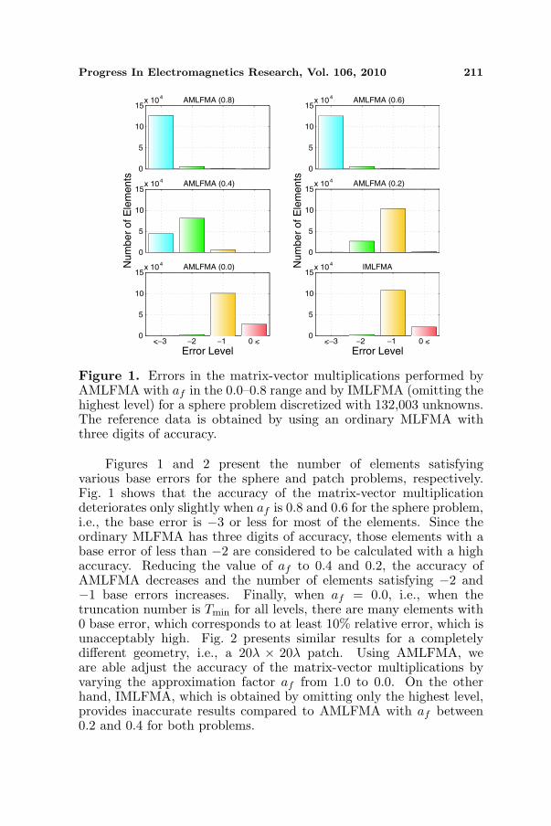
Figure 1. Errors in the matrix-vector multiplications performed byAMLFMA with af in the 0.0–0.8 range and by IMLFMA (omitting thehighest level) for a sphere problem discretized with 132,003 unknowns.The reference data is obtained by using an ordinary MLFMA withthree digits of accuracy.

Figures 1 and 2 present the number of elements satisfyingvarious base errors for the sphere and patch problems, respectively.Fig. 1 shows that the accuracy of the matrix-vector multiplicationdeteriorates only slightly when af is 0.8 and 0.6 for the sphere problem,i.e., the base error is −3 or less for most of the elements. Since theordinary MLFMA has three digits of accuracy, those elements with abase error of less than −2 are considered to be calculated with a highaccuracy. Reducing the value of af to 0.4 and 0.2, the accuracy ofAMLFMA decreases and the number of elements satisfying −2 and−1 base errors increases. Finally, when af = 0.0, i.e., when thetruncation number is Tmin for all levels, there are many elements with0 base error, which corresponds to at least 10% relative error, which isunacceptably high. Fig. 2 presents similar results for a completelydifferent geometry, i.e., a 20λ × 20λ patch. Using AMLFMA, weare able adjust the accuracy of the matrix-vector multiplications byvarying the approximation factor af from 1.0 to 0.0. On the otherhand, IMLFMA, which is obtained by omitting only the highest level,provides inaccurate results compared to AMLFMA with af between0.2 and 0.4 for both problems.


0

5

10

15x 10

4AMLFMA (0.8)

0

5

10

15x 10

4AMLFMA (0.6)

0

5

10

15x 10

4AMLFMA (0.4)

Num

ber

of E

lem

ents

0

5

10

15x 10

4AMLFMA (0.2)

Num

ber

of E

lem

ents

−2 −1 0

5

10

15x 10

4AMLFMA (0.0)

Base Error<−3 −2 −1

0

5

10

15x 10

4IMLFMA

Base Error<−3 0 <0 <

Figure 2. Errors in the matrix-vector multiplications performed byAMLFMA with af in the 0.0–0.8 range and by IMLFMA (omitting thehighest level) for a patch problem discretized with 137,792 unknowns.The reference data is obtained by using an ordinary MLFMA withthree digits of accuracy.

Figures 1 and 2 show that we obtain relatively accurate matrix-vector multiplications by AMLFMA when using af in the 0.2–0.4range. This cannot be predicted by the excess bandwidth formulain (3), which suggests significantly large truncation numbers, as listedin Table 1. This is because the excess bandwidth formula is basedon the worst-case scenario for the positions of the basis and testingfunctions inside the clusters [11]. In fact, the ordinary MLFMA mustuse the truncation numbers obtained with (3) to guarantee the desiredlevel of accuracy. However, for a typical problem, there are manyinteractions that can be computed accurately using lower truncationnumbers. We employ those interactions in AMLFMA, which can beused to construct powerful preconditioners. Due to the nature ofpreconditioning, perfect accuracy is not required, instead, the fastestpossible solution with the least possible approximation is desired.

Finally, Table 2 lists the processing time required for a matrix-vector multiplication performed by the ordinary MLFMA, AMLFMA,and IMLFMA, measured on a parallel computer system containing 16AMD Opteron 870 processors. For both sphere and patch problems,


Table 2. Processing time (seconds) for a single matrix-vectormultiplication.

Problem-Unknowns MLFMAAMLFMA

IMLFMA0.8 0.6 0.4 0.2 0.0

Sphere-132,003 34.9 28.3 23.2 19.8 16.0 13.0 32.4

Patch-137,792 24.5 19.4 15.2 12.8 10.1 8.1 21.6

AMLFMA with af = 0.2 provides a significant acceleration by reducingprocessing time more than 50% compared with the ordinary MLFMA.We also note that the speedup provided by IMLFMA is less than thespeedup provided by AMLFMA, even when af = 0.8.

4. PRECONDITIONERS BUILT FROM NEAR-FIELDMATRICES

In MLFMA, there are O(N) near-field interactions available forthe construction of various preconditioners. For example, usingthe self-interactions of the lowest-level clusters leads to the block-diagonal (BD) preconditioner, which effectively reduces the numberof iterations for the combined-field integral equation (CFIE) [1, 15].On the other hand, the BD preconditioner usually decelerates theiterative solutions of the electric-field integral equation (EFIE) [15]. Inaddition, for large problems involving complicated objects, accelerationprovided by the BD preconditioner may not be sufficient, even whenthe problems are formulated with CFIE. For the efficient solution ofthose problems, it is necessary to construct better preconditioners [16]by using all of the available near-field interactions instead of using onlythe diagonal blocks.

One of the most common preconditioning techniques based onthe sparse matrices is the incomplete LU (ILU) method [17]. Thisis a forward-type preconditioning technique, where the preconditionermatrix M approximates the system matrix, and we solve for

M−1 · Z · a = M

−1 · v (left preconditioning) (7)

or (Z ·M−1

)· (M · a)

= v (right preconditioning), (8)

instead of the original matrix equation Z · a = v. In (7) and (8),the solution of M · x = y for a given y should be cheaper than thesolution of the original matrix equation. During the factorization of


the preconditioner matrix, the ILU method sacrifices some of the fill-insand provides an approximation to the near-field matrix, i.e.,

M = L · U ≈ ZNF . (9)

Recently, we showed that an ILU preconditioner without a thresholdprovides an inexpensive and good approximation to the solution of thenear-field matrix for CFIE, hence it reduces the iteration counts andsolution times substantially [18]. For ill-conditioned EFIE matrices,however, ILUT (i.e., threshold-based ILU) with pivoting [19] is requiredto prevent the potential instability. Other successful adoptions of theILU preconditioners are presented by Lee et al. [20].

Despite the remarkable success of the ILU preconditioners, theyare limited to sequential implementations due to difficulties in paral-lelizing their factorization algorithms and forward-backward solutions.Hence, the sparse-approximate-inverse (SAI) preconditioner that iswell-suited for parallel implementations has been more preferable forthe solution of large-scale electromagnetics problems [14, 21, 22]. TheSAI preconditioner is based on a backward-type scheme, where the in-verse of the system matrix is directly approximated, i.e., M ≈ Z

−1. InMLFMA, only the near-field matrix is considered [23], and we minimize

∥∥I −M · ZNF

∥∥F

, (10)

where ‖ · ‖F represents the Frobenius norm. Using the pattern ofthe near-field matrix for the nonzero pattern of M provides someadvantages by decreasing the number of QR factorizations requiredduring the minimization in (10) [14]. In parallel implementations, weuse a row-wise partitioning to distribute the near-field interactionsamong the processors. Therefore, left-preconditioning must be usedto accelerate the iterative solutions with the SAI preconditioner.However, right-preconditioning can also be used for the symmetricmatrix equations derived from EFIE [22].

Recently, we showed that the SAI preconditioner is useful inreducing the iteration counts for closed and complicated surfacesformulated with CFIE, as well as open surfaces formulated withEFIE. However, for EFIE, the SAI preconditioner is less successfulthan the ILU methods, although they are based on the same near-field matrix. As a remedy, we use an inner-outer scheme [6] byemploying the SAI preconditioner to accelerate the iterative solutionof the near-field system, which is then used as a preconditioner for thefull matrix equation [24]. The resulting forward-type preconditioneris called the iterative near-field (INF) preconditioner. Contrary tothe ILU preconditioners, which approximate the near-field matrix(M ≈ ZNF ), the INF preconditioner employs the near-field matrix


exactly (M = ZNF ), but the preconditioner system is solved iterativelyand approximately. Since the preconditioner is changed during theiterations, a flexible Krylov-subspace method should be used for theouter solutions [19]. In the next section, we introduce a robustpreconditioning technique, which is based on a similar inner-outerscheme, but this time we employ AMLFMA for the inner solutionsto construct more effective preconditioners.

5. ITERATIVE PRECONDITIONING BASED ONAMLFMA

Preconditioners that are based on the near-field interactions can beinsufficient to accelerate the iterative solutions of large-scale problems,especially those formulated with EFIE. For more efficient solutions,it is possible to use the far-field interactions in addition to the near-field interactions and construct more effective preconditioners. Thiscan be achieved by using flexible solvers and employing approximateand ordinary versions of MLFMA in an inner-outer scheme. Usinga reasonable approximation for the inner solutions, the number ofouter iterations can be reduced substantially. In addition to moreefficient solutions, the inner-outer scheme prevents numerical errorsthat arise because of the deviations of the computed residual from thetrue residual by significantly decreasing the number of outer iterations.This is because the “residual gap,” i.e., the difference between the trueand computed residuals, increases with the number of iterations [25].Another benefit of the reduction in iteration counts appears when theiterative solutions are performed with the generalized minimal residual(GMRES) algorithm, which is usually an optimal method for EFIE interms of the processing time [14, 18]. Even though flexible variants ofGMRES, namely, FGMRES [19] or GMRESR [26], require the storageof two vectors per iteration instead of one, nested solutions requiresignificantly less memory than the ordinary GMRES solutions sincenested solutions dramatically reduce the iteration counts.

There are many factors that affect the performance of an inner-outer scheme, such as the primary preconditioning operator, the choiceof the inner solver and the secondary preconditioner to accelerate theinner solutions, and the inner stopping criteria. Now, we discuss thesefactors in detail.

5.1. Preconditioning Operator

In an extreme case, one can use the full matrix itself as a preconditionerby employing the ordinary MLFMA to perform the matrix-vector


multiplications for the inner solutions. On the other hand, an inner-outer scheme usually increases the total number of matrix-vectormultiplications compared to the ordinary solutions [25]. In addition, anapproximate solution instead of an ordinary solution can be sufficientto construct a robust preconditioner. As discussed in Section 3,AMLFMA is an appropriate choice to perform the inner solutions.By using the approximation factor af , the accuracy of AMLFMA canbe adjusted to achieve a maximum overall efficiency.

5.2. Inner Solver and the Secondary Preconditioner

For the inner solutions, GMRES is preferable due to its rapidconvergence in a small number of iterations. The inner solutionsare also accelerated by using a secondary preconditioner based onthe near-field interactions. Among the various choices discussed inSection 4, we prefer the SAI preconditioner, which effectively increasesthe convergence rate, especially in the early stages of the iterativesolutions [14].

5.3. Inner Stopping Criteria

The relative residual error εin and the upper limit for the numberof inner iterations jin

max are also important parameters that affect theoverall efficiency of the inner-outer scheme. Van den Eshof et al. [25]showed that fixing εin is nearly optimal if relaxation is not applied.However, even 0.1 (10%) residual error can cause a significant numberof inner iterations for large-scale problems. Therefore, in addition toεin, the maximum number of iterations jin

max should be set carefullyto avoid unnecessary iterations during the inner solutions. For largeproblems, a small value of jin

max is more likely to keep the inner iterationcounts under control than a large value of εin.

6. NUMERICAL RESULTS

Finally, we demonstrate the performance of the proposed inner-outer scheme using AMLFMA, compared to the solutions acceleratedwith BD, SAI, and INF preconditioners. Fortran 90 programminglanguage is used for all implementations. Solutions are performedon a distributed-memory parallel computer containing Intel XeonHarpertown processors with 3.0 GHz clock rate. A total of 32cores located in 16 nodes (2 cores per node) are used, and thenodes are connected via an Infiniband network. A hierarchicalpartitioning strategy is used for the parallelization of MLFMA [3].


Iterative solvers, namely, GMRES and FGMRES, are provided by thePETSc library [27]. In all solutions, matrix-vector multiplicationsare performed by MLFMA with three digits of accuracy. For theinner solutions with AMLFMA, the target residual error and theapproximation factor are set to 10−1 and 0.2, respectively. To avoidunnecessary work, inner solutions are stopped at maximum 10thiteration (jin

max = 10). For the INF preconditioner, however, the targetresidual error for the inner solutions is in the range of 10−2 to 10−1,whereas the maximum number of iterations is set to between 3 and5, depending on the problem. A small number of inner iterationsis usually sufficient for INF since the SAI preconditioner used toaccelerate the inner solutions provides a good approximation to ZNF .

Parameters for the preconditioners are determined by testingthe implementations on a wide class of problems and choosing theoptimal combination to minimize the total processing time for eachpreconditioner. For example, by setting the approximation factor to0.2 in AMLFMA, most of the matrix elements are calculated with lessthan 10% error. Then, using 10−1 residual error for the inner iterationsprovides the best performance. Choosing a smaller error thresholdleads to unnecessary iterations and a larger error threshold wastes therelatively high accuracy of AMLFMA. Setting the maximum number ofiterations to more than 10 increases the processing time, even thoughthe accuracy of the inner solutions is not improved significantly.

EFIE is notorious for generating ill-conditioned matrix equations,which are difficult to solve iteratively, especially when the problemsize is large [18, 28]. Therefore, the proposed inner-outer schemeemploying AMLFMA is particularly useful for open surfaces that mustbe formulated with EFIE. In addition, we show that the iterativesolutions of complicated problems involving closed surfaces that areformulated with CFIE are also improved by the proposed method.

6.1. EFIE Results

Figure 3 presents three different metallic objects involving opensurfaces, namely, a square patch (P), a half sphere (HS), and areflector antenna (RA). The patch is illuminated by a horizontally-polarized plane wave propagating at 45◦ angle from the normal ofthe patch. The half sphere and the reflector antenna are illuminatedby plane waves propagating along the axes of symmetry of theseobjects. Discretizations of the objects for various frequencies lead tolarge matrix equations with millions of unknowns, as listed in Table 3.Dimensions of the objects in terms of the wavelength and the numberof active levels (L) in MLFMA are also listed in Table 3.


Patch (P) Half Sphere (HS)

Reflector Antenna (RA)

Figure 3. Metallic objects modeled with open surfaces.

Table 3. Electromagnetics problems involving open metallic objects.

ProblemFrequency Size MLFMA Number of

(GHz) (λ) Levels Unknowns

P1 96 96 8 3,062,400

P2 128 128 8 5,511,680

P3 192 192 9 12,253,440

HS1 96 96 8 3,838,496

HS2 128 128 8 6,535,168

HS3 192 192 9 15,356,992

RA1 32 107 8 2,991,067

RA2 48 160 9 6,849,398

RA3 64 214 9 11,967,620

Table 4 presents the number of iterations and the processing timefor the solutions of the problems in Table 3. We observe that using theINF preconditioner accelerates the solutions significantly compared tothe SAI preconditioner used alone. Employing the inner-outer schemewith AMLFMA further reduces the processing time, and we are able tosolve the largest problem discretized with about 12 million unknownsin less than 7 hours. Although not shown in Table 4, the memoryrequired for the iterative algorithm is also reduced substantially by theproposed method since the memory requirements of both GMRES andFGMRES increase with the number of iterations. As an example, forthe solution of P3 with SAI, GMRES requires 2614 MB per processor.Using an inner-outer scheme and AMLFMA, the memory requirementis reduced to 820 MB.


Table 4. Processing time (seconds) and the number of iterationsafor the solution of electromagnetics problems involving open metallicobjects.

ProblemSAIb SAI INF AMLFMA

Setup Outer Time Outer Inner Time Outer Inner Time

P1 132 194 6,225 131 391 4,393 35 345 3,278

P2 308 234 27,902 160 478 19,620 43 425 9,860

P3 1,136 276 36,677 174 868 25,650 52 516 17,454

HS1 350 480 23,458 367 1,101 18,374 68 680 11,085

HS2 839 546 66,778 406 1,218 51,285 75 750 23,143

HS3 5,620 357 59,734 276 1,380 48,786 51 510 31,740

RA1 201 200 7,276 138 408 5,138 33 327 4,233

RA2 671 252 31,784 172 509 22,404 42 417 13,746

RA3 2,077 336 43,912 228 1,138 32,710 57 567 24,595

aThe relative residual error is 10−3 for HS3 and RA3, and 10−6 for other

problems.bSetup of the SAI preconditioner is also required for INF and AMLFMA.

Helicopter (H) Flamme (F)

Figure 4. Metallic objects modeled with closed surfaces.

6.2. CFIE Results

Figure 4 presents two objects modeled with closed conducting surfaces,namely, a helicopter (H) and a stealth airborne target namedFlamme (F) [29]. The Flamme is illuminated by a plane wavepropagating towards the nose of the target, whereas the helicopteris illuminated from the top. Electromagnetics problems involvingthose objects in Fig. 4 and listed in Table 5 are formulated withCFIE (α = 0.2). Table 6 presents the number of iterations andthe processing time when the solutions are accelerated with the BDand SAI preconditioners, as well as the inner-outer scheme using


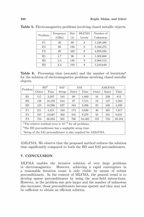
Table 5. Electromagnetics problems involving closed metallic objects.

ProblemFrequency Size MLFMA Number of

(GHz) (λ) Levels Unknowns

F1 40 80 8 1,248,480

F2 60 120 8 3,166,272

F3 80 160 9 4,993,920

H1 1.7 96 8 1,302,660

H2 2.4 136 9 2,968,512

H3 3.4 193 9 5,210,640

Table 6. Processing time (seconds) and the number of iterationsafor the solution of electromagnetics problems involving closed metallicobjects.

ProblemBDb SAIc SAI AMLFMA

Outer Time Setup Outer Time Outer Inner Time

H1 117 2,287 183 90 1,869 16 239 813

H2 138 10,192 644 97 7,515 19 137 2,562

H3 125 10,986 627 104 9,386 25 240 4,938

F1 211 4,451 163 174 3,836 40 305 1,917

F2 347 10,087 402 316 9,276 58 331 6,641

F3 724 66,094 505 706 64,365 125 733 28,593

aThe relative residual error is 10−6 for all problems.bThe BD preconditioner has a negligible setup time.cSetup of the SAI preconditioner is also required for AMLFMA.

AMLFMA. We observe that the proposed method reduces the solutiontime significantly compared to both the BD and SAI preconditioners.

7. CONCLUSION

MLFMA enables the iterative solution of very large problemsin electromagnetics. However, achieving a rapid convergence ina reasonable iteration count is only viable by means of robustpreconditioners. In the context of MLFMA, the general trend is todevelop sparse preconditioners by using the near-field interactions.However, as the problem size gets larger and the number of unknownsalso increases, those preconditioners become sparser and they may notbe sufficient to obtain an efficient solution.


In this paper, we propose an inner-outer scheme to improveiterative solutions with MLFMA. For the inner solutions, matrix-vector multiplications are performed efficiently by AMLFMA, whichis obtained by systematically reducing the accuracy of the ordinaryMLFMA. We show that the resulting solver accelerates the iterativesolutions of electromagnetics problems involving open and closedgeometries formulated with EFIE and CFIE, respectively.

ACKNOWLEDGMENT

This work was supported by the Scientific and Technical ResearchCouncil of Turkey (TUBITAK) under Research Grants 105E172 and107E136, the Turkish Academy of Sciences in the framework ofthe Young Scientist Award Program (LG/TUBA-GEBIP/2002-1-12),and by contracts from ASELSAN and SSM. Ozgur Ergul was alsosupported by a Research Starter Grant provided by the Faculty ofScience at the University of Strathclyde.

REFERENCES

1. Song, J., C.-C. Lu, and W. C. Chew, “Multilevel fast multipolealgorithm for electromagnetic scattering by large complexobjects,” IEEE Trans. Antennas Propagat., Vol. 45, No. 10, 1488–1493, Oct. 1997.

2. Coifman, R., V. Rokhlin, and S. Wandzura, “The fast multipolemethod for the wave equation: A pedestrian prescription,” IEEEAntennas Propag. Mag., Vol. 35, No. 3, 7–12, Jun. 1993.

3. Ergul, O. and L. Gurel, “A hierarchical partitioning strategy forefficient parallelization of the multilevel fast multipole algorithm,”IEEE Trans. Antennas Propagat., Vol. 57, No. 6, 1740–1750,Jun. 2009.

4. Taboada, J. M., M. G. Araujo, J. M. Bertolo, L. Landesa,F. Obelleiro, and J. L. Rodriguez, “MLFMA-FFT parallel algo-rithm for the solution of large-scale problems in electromagnetics,”Progress In Electromagnetics Research, Vol. 105, 15–30, 2010.

5. Bouras, A. and V. Fraysse, “Inexact matrix-vector products inKrylov methods for solving linear systems: A relaxation strategy,”SIAM J. Matrix Anal. Appl., Vol. 26, No. 3, 660–678, 2005.

6. Simoncini, V. and D. B. Szyld, “Flexible inner-outer Krylovsubspace methods,” SIAM J. Numer. Anal., Vol. 40, No. 6, 2219–2239, 2003.


7. Ding, D. Z., R. S. Chen, and Z. H. Fan, “SSOR preconditionedinner-outer flexible GMRES method for MLFMA analysisof scattering of open objects,” Progress In ElectromagneticsResearch, Vol. 89, 339–357, 2009.

8. Chew, W. C., J.-M. Jin, E. Michielssen, and J. Song, Fast andEfficient Algorithms in Computational Electromagnetics, ArtechHouse, Boston, MA, 2001.

9. Rao, S. M., D. R. Wilton, and A. W. Glisson, “Electromagneticscattering by surfaces of arbitrary shape,” IEEE Trans. AntennasPropagat., Vol. 30, No. 3, 409–418, May 1982.

10. Koc, S., J. M. Song, and W. C. Chew, “Error analysis for thenumerical evaluation of the diagonal forms of the scalar sphericaladdition theorem,” SIAM J. Numer. Anal., Vol. 36, No. 3, 906–921, 1999.

11. Hastriter, M. L., S. Ohnuki, and W. C. Chew, “Error control of thetranslation operator in 3D MLFMA,” Microwave Opt. Technol.Lett., Vol. 37, No. 3, 184–188, Mar. 2003.

12. Ergul, O. and L. Gurel, “Optimal interpolation of translationoperator in multilevel fast multipole algorithm,” IEEE Trans.Antennas Propagat., Vol. 54, No. 12, 3822–3826, Dec. 2006.

13. Brandt, A., “Multilevel computations of integral transformsand particle interactions with oscillatory kernels,” Comp. Phys.Comm., Vol. 65, 24–38, Apr. 1991.

14. Carpentieri, B., I. S. Duff, L. Giraud, and G. Sylvand,“Combining fast multipole techniques and an approximate inversepreconditioner for large electromagnetism calculations,” SIAM J.Sci. Comput., Vol. 27, No. 3, 774–792, 2005.

15. Ergul, O. and L. Gurel, “Iterative solutions of hybrid integralequations for coexisting open and closed surfaces,” IEEE Trans.Antennas Propag., Vol. 57, No. 6, 1751–1758, Jun. 2009.

16. Araujo, M. G., J. M. Bertolo, F. Obelleiro, and J. L. Rodriguez,“Geometry based preconditioner for radiation problems involvingwire and surface basis functions,” Progress In ElectromagneticsResearch, Vol. 93, 29–40, 2009.

17. Benzi, M., “Preconditioning techniques for large linear systems:A survey,” J. Comput. Phys., Vol. 182, No. 2, 418–477, Nov. 2002.

18. Malas, T. and L. Gurel, “Incomplete LU preconditioningwith the multilevel fast multipole algorithm for electromagneticscattering,” SIAM J. Sci. Comput., Vol. 29, No. 4, 1476–1494,Jun. 2007.

19. Saad, Y., Iterative Methods for Sparse Linear Systems, SIAM,


Philadelphia, 2003.20. Lee, J., J. Zhang, and C.-C. Lu, “Incomplete LU preconditioning

for large scale dense complex linear systems from electromagneticwave scattering problems,” J. Comput. Phys., Vol. 185, No. 1,158–175, Feb. 2003.

21. Lee, J., J. Zhang, and C.-C. Lu, “Sparse inverse preconditioning ofmultilevel fast multipole algorithm for hybrid integral equations inelectromagnetics,” IEEE Trans. Antennas and Propagat., Vol. 52,No. 9, 2277–2287, Sep. 2004.

22. Malas, T. and L. Gurel, “Accelerating the multilevel fastmultipole algorithm with the sparse-approximate-inverse (SAI)preconditioning,” SIAM J. Sci. Comput., Vol. 31, No. 3, 1968–1984, Mar. 2009.

23. Ding, D. Z., R. S. Chen, and Z. H. Fan, “An efficient SAIpreconditioning technique for higher order hierarchical MLFMAimplementation,” Progress In Electromagnetics Research, Vol. 88,255–273, 2008.

24. Gurel, L. and T. Malas, “Iterative near-field (INF) preconditionerfor the multilevel fast multipole algorithm,” SIAM J. Sci.Comput., accepted for publication.

25. Van den Eshof, J., G. L. G. Sleijpen, and M. B. van Gijzen,“Relaxation strategies for nested Krylov methods,” J. Comput.Appl. Math., Vol. 177, No. 2, 347–365, May 2005.

26. Van der Vorst, H. and C. Vuik, “GMRESR: A family of nestedGMRES methods,” Numer. Linear Algebra Appl., Vol. 1, No. 4,369–386, Jul. 1994.

27. Balay, S., W. D. Gropp, L. C. McInnes, and B. F. Smith,PETSc Users Manual, Tech. Report ANL-95/11 — Revision 2.1.5,Argonne National Laboratory, 2004.

28. Carpentieri, B., I. S. Duff, and L. Giraud, “Experiments withsparse preconditioning of dense problems from electromagneticapplications,” Tech. Report TR/PA/00/04, CERFACS, Toulouse,France, 1999.

29. Gurel, L., H. Bagcı, J.-C. Castelli, A. Cheraly, and F. Tardivel,“Validation through comparison: Measurement and calculation ofthe bistatic radar cross section of a stealth target,” Radio Science,Vol. 38, No. 3, 12-1–12-10, Jun. 2003.

Documents

SOLUTIONS OF LARGE-SCALE ELECTROMAGNETICS PROBLEMS USING ... · Progress In Electromagnetics Research, Vol. 106, 203{223, 2010 SOLUTIONS OF LARGE-SCALE ELECTROMAGNETICS PROBLEMS USING