Embed Size (px)
Citation preview

SolutionsManual
Hadi SaadatProfessor of Electrical EngineeringMilwaukee School of Engineering
Milwaukee, Wisconsin
McGraw-Hill, Inc.


CONTENTS
1 THE POWER SYSTEM: AN OVERVIEW 1
2 BASIC PRINCIPLES 5
3 GENERATOR AND TRANSFORMER MODELS;THE PER-UNIT SYSTEM 25
4 TRANSMISSION LINE PARAMETERS 52
5 LINE MODEL AND PERFORMANCE 68
6 POWER FLOW ANALYSIS 107
7 OPTIMAL DISPATCH OF GENERATION 147
8 SYNCHRONOUS MACHINE TRANSIENT ANALYSIS 170
9 BALANCED FAULT 181
10 SYMMETRICAL COMPONENTS AND UNBALANCED FAULT 208
11 STABILITY 244
12 POWER SYSTEM CONTROL 263
i
CHAPTER1 PROBLEMS
1.1 The demand estimation is the starting point for planning the future electricpower supply. The consistency of demand growth over the years has led to numer-ous attempts to fit mathematical curves to this trend. One of the simplest curvesis
P = P0ea(t−t0)
wherea is the average per unit growth rate,P is the demand in yeart, andP0 isthe given demand at yeart0.
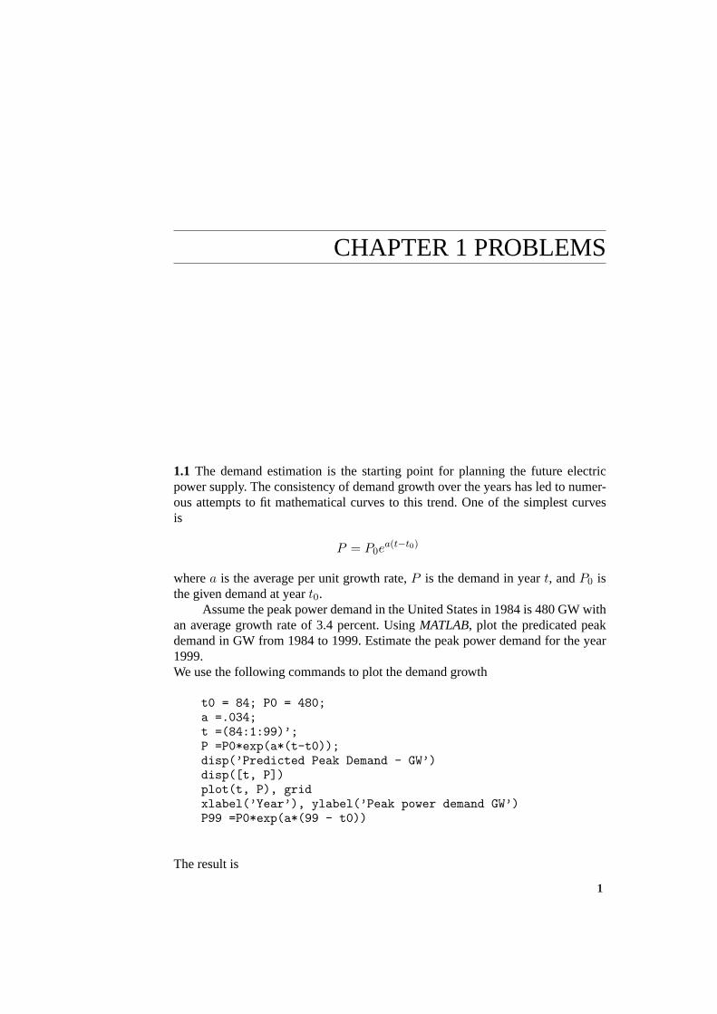
Assume the peak power demand in the United States in 1984 is 480 GW withan average growth rate of 3.4 percent. UsingMATLAB, plot the predicated peakdemand in GW from 1984 to 1999. Estimate the peak power demand for the year1999.We use the following commands to plot the demand growth
t0 = 84; P0 = 480;a =.034;t =(84:1:99)’;P =P0*exp(a*(t-t0));disp(’Predicted Peak Demand - GW’)disp([t, P])plot(t, P), gridxlabel(’Year’), ylabel(’Peak power demand GW’)P99 =P0*exp(a*(99 - t0))
The result is
1
2 CONTENTS
Predicted Peak Demand - GW84.0000 480.000085.0000 496.600686.0000 513.775387.0000 531.544188.0000 549.927389.0000 568.946390.0000 588.623191.0000 608.980492.0000 630.041893.0000 651.831594.0000 674.374095.0000 697.697896.0000 721.827497.0000 746.791698.0000 772.619099.0000 799.3398
P99 =
799.3398
The plot of the predicated demand is shown n Figure 1.
450
500
550
600
650
700
750
800
PeakPowerDemandGW
84 86 88 90 92 94 96 98 100
Year
........................................
.........................................
.......................................
.......................................
.....................................
....................................
.....................................
....................................
...................................
..................................
..................................
.................................
................................
................................
................................
...............................
...............................
..............................
..............................
............................
.......
.
.
.
.
.
.
.
.
.
.
.
.
.
.
.
.
.
.
.
.
.
.
.
.
.
.
.
.
.
.
.
.
.
.
.
.
.
.
.
.
.
.
.
.
.
.
.
.
.
.
.
.
.
.
.
.
.
.
.
.
.
.
.
.
.
.
.
.
.
.
.
.
.
.
.
.
.
.
.
.
.
.
.
.
.
.
.
.
.
.
.
.
.
.
.
.
.
.
.
.
.
.
.
.
.
.
.
.
.
.
.
.
.
.
.
.
.
.
.
.
.
.
.
.
.
.
.
.
.
.
.
.
.
.
.
.
.
.
.
.
.
.
.
.
.
.
.
.
.
.
.
.
.
.
.
.
.
.
.
.
.
.
.
.
.
.
.
.
.
.
.
.
.
.
.
.
.
.
.
.
.
.
.
.
.
.
.
.
.
.
.
.
.
.
.
.
.
.
.
.
.
.
.
.
.
.
.
.
.
.
.
.
.
.
.
.
.
.
.
.
.
.
.
.
.
.
.
.
.
.
.
.
.
.
.
.
.
.
.
.
.
.
.
.
.
.
.
.
. . . . . . . . . . . . . . . . . . . . . . . . . . . . . . . . . . . . . . . . . . . . . . . . . . . . . . . .
. . . . . . . . . . . . . . . . . . . . . . . . . . . . . . . . . . . . . . . . . . . . . . . . . . . . . . . .
. . . . . . . . . . . . . . . . . . . . . . . . . . . . . . . . . . . . . . . . . . . . . . . . . . . . . . . .
. . . . . . . . . . . . . . . . . . . . . . . . . . . . . . . . . . . . . . . . . . . . . . . . . . . . . . . .
. . . . . . . . . . . . . . . . . . . . . . . . . . . . . . . . . . . . . . . . . . . . . . . . . . . . . . . .
. . . . . . . . . . . . . . . . . . . . . . . . . . . . . . . . . . . . . . . . . . . . . . . . . . . . . . . .
. . . . . . . . . . . . . . . . . . . . . . . . . . . . . . . . . . . . . . . . . . . . . . . . . . . . . . . .
. . . . . . . . . . . . . . . . . . . . . . . . . . . . . . . . . . . . . . . . . . . . . . . . . . . . . . . .
FIGURE 1Peak Power Demand for Problem 1.1
1.2 In a certain country, the energy consumption is expected to double in 10 years.

CONTENTS 3
Assuminga simple exponential growth given by
P = P0eat
calculate the growth ratea.
2P0 = P0e10a
ln 2 = 10a
Solving fora, we have
a =0.69310
= 0.0693 = 6.93%
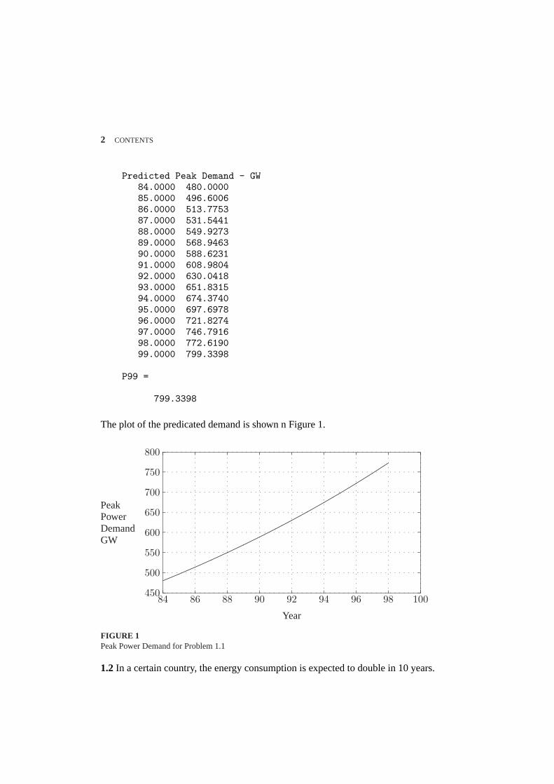
1.3. The annual load of a substation is given in the following table. During eachmonth, the power is assumed constant at an average value. UsingMATLABandthebarcycle function, obtain a plot of the annual load curve. Write the necessarystatements to find the average load and the annual load factor.
Annual System LoadInterval – Month Load– MWJanuary 8February 6March 4April 2May 6June 12July 16August 14September 10October 4November 6December 8
Thefollowing commands
data = [ 0 1 81 2 62 3 43 4 24 5 65 6 12
4 CONTENTS
6 7 167 8 148 9 109 10 410 11 611 12 8];
P = data(:,3); % Column array of loadDt = data(:, 2) - data(:,1); % Column array of demand intervalW = P’*Dt; % Total energy, area under the curvePavg = W/sum(Dt) % Average loadPeak = max(P) % Peak loadLF = Pavg/Peak*100 % Percent load factorbarcycle(data) % Plots the load cyclexlabel(’time, month’), ylabel(’P, MW’), grid
result in
Pavg =8
Peak =16
LF =50
0
2
4
6
8
10
12
14
16
PMW
0 2 4 6 8 10 12
time, month
..................................................................................................................................................................................................................................................................................................................................................................................................................................................................................................................................................................................
........
........
........
........
........
........
........
........
........
........
........
........
........
........
........
........
........
..........................................................................................................................................................................................................................................................................................................................................................................................................................................................................................................................................................................................................................................................................................................................................
........
........
........
........
........
..............................................................................................................................................................................
.
.
.
.
.
.
.
.
.
.
.
.
.
.
.
.
.
.
.
.
.
.
.
.
.
.
.
.
.
.
.
.
.
.
.
.
.
.
.
.
.
.
.
.
.
.
.
.
.
.
.
.
.
.
.
.
.
.
.
.
.
.
.
.
.
.
.
.
.
.
.
.
.
.
.
.
.
.
.
.
.
.
.
.
.
.
.
.
.
.
.
.
.
.
.
.
.
.
.
.
.
.
.
.
.
.
.
.
.
.
.
.
.
.
.
.
.
.
.
.
.
.
.
.
.
.
.
.
.
.
.
.
.
.
.
.
.
.
.
.
.
.
.
.
.
.
.
.
.
.
.
.
.
.
.
.
.
.
.
.
. . . . . . . . . . . . . . . . . . . . . . . . . . . . . . . . . . . . . . . . . . . . . . . . . . . . . . . . . . .
. . . . . . . . . . . . . . . . . . . . . . . . . . . . . . . . . . . . . . . . . . . . . . . . . . . . . . . . . . .
. . . . . . . . . . . . . . . . . . . . . . . . . . . . . . . . . . . . . . . . . . . . . . . . . . . . . . . . . . .
. . . . . . . . . . . . . . . . . . . . . . . . . . . . . . . . . . . . . . . . . . . . . . . . . . . . . . . . . . .
. . . . . . . . . . . . . . . . . . . . . . . . . . . . . . . . . . . . . . . . . . . . . . . . . . . . . . . . . . .
. . . . . . . . . . . . . . . . . . . . . . . . . . . . . . . . . . . . . . . . . . . . . . . . . . . . . . . . . . .
. . . . . . . . . . . . . . . . . . . . . . . . . . . . . . . . . . . . . . . . . . . . . . . . . . . . . . . . . . .
FIGURE 2Monthly load cycle for Problem 1.3
CHAPTER2 PROBLEMS
2.1.Modify the program in Example 2.1 such that the following quantities can beentered by the user:The peak amplitudeVm, and the phase angleθv of the sinusoidal supplyv(t) =Vm cos(ωt + θv). The impedance magnitudeZ, and its phase angleγ of the load.The program should produce plots fori(t), v(t), p(t), pr(t) andpx(t), similar toExample 2.1. Run the program forVm = 100 V, θv = 0 and the following loads:
An inductive load,Z = 1.256 60 ΩA capacitive load,Z = 2.0 6 −30 ΩA resistive load, Z = 2.56 0 Ω
(a) Frompr(t) andpx(t) plots, estimate the real and reactive power for each load.Draw a conclusion regarding the sign of reactive power for inductive and capaci-tive loads.(b) Using phasor values of current and voltage, calculate the real and reactive powerfor each load and compare with the results obtained from the curves.(c) If the above loads are all connected across the same power supply, determinethe total real and reactive power taken from the supply.
The following statements are used to plot the instantaneous voltage, current, andthe instantaneous terms given by(2-6) and (2-8).
Vm = input(’Enter voltage peak amplitude Vm = ’);thetav =input(’Enter voltage phase angle in degree thetav = ’);Vm = 100; thetav = 0; % Voltage amplitude and phase angleZ = input(’Enter magnitude of the load impedance Z = ’);gama = input(’Enter load phase angle in degree gama = ’);thetai = thetav - gama; % Current phase angle in degree
5
6 CONTENTS
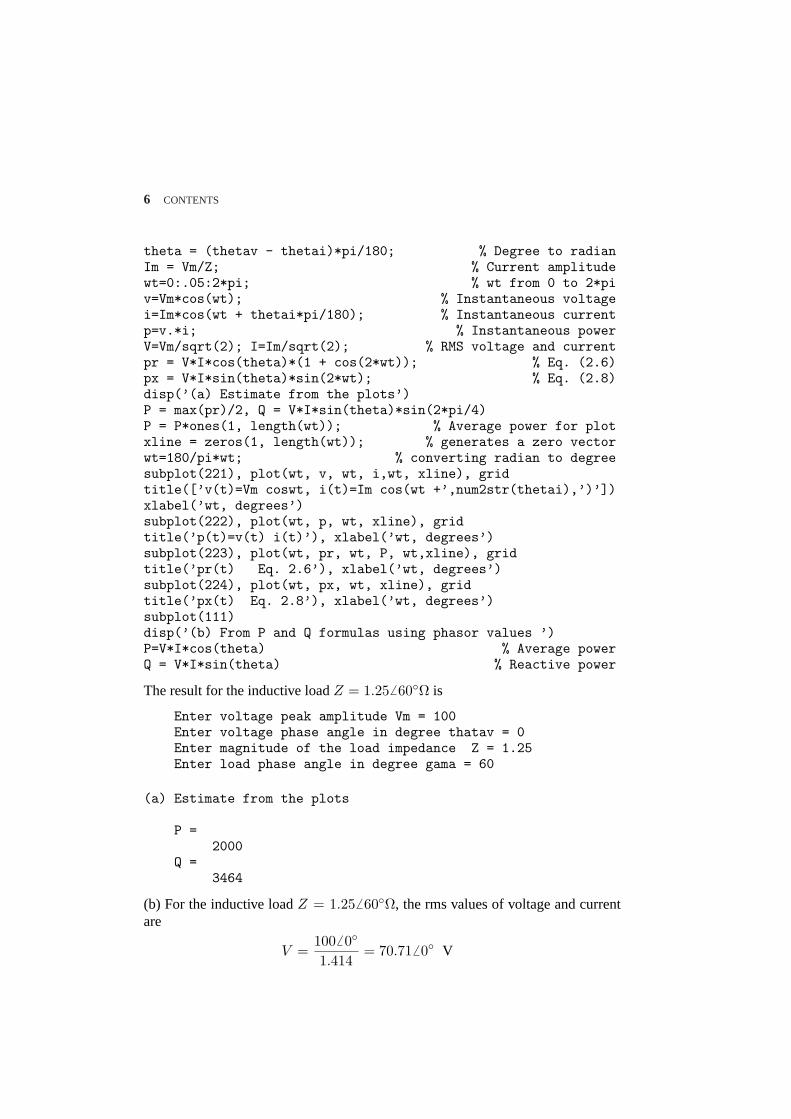
theta = (thetav - thetai)*pi/180; % Degree to radianIm = Vm/Z; % Current amplitudewt=0:.05:2*pi; % wt from 0 to 2*piv=Vm*cos(wt); % Instantaneous voltagei=Im*cos(wt + thetai*pi/180); % Instantaneous currentp=v.*i; % Instantaneous powerV=Vm/sqrt(2); I=Im/sqrt(2); % RMS voltage and currentpr = V*I*cos(theta)*(1 + cos(2*wt)); % Eq. (2.6)px = V*I*sin(theta)*sin(2*wt); % Eq. (2.8)disp(’(a) Estimate from the plots’)P = max(pr)/2, Q = V*I*sin(theta)*sin(2*pi/4)P = P*ones(1, length(wt)); % Average power for plotxline = zeros(1, length(wt)); % generates a zero vectorwt=180/pi*wt; % converting radian to degreesubplot(221), plot(wt, v, wt, i,wt, xline), gridtitle([’v(t)=Vm coswt, i(t)=Im cos(wt +’,num2str(thetai),’)’])xlabel(’wt, degrees’)subplot(222), plot(wt, p, wt, xline), gridtitle(’p(t)=v(t) i(t)’), xlabel(’wt, degrees’)subplot(223), plot(wt, pr, wt, P, wt,xline), gridtitle(’pr(t) Eq. 2.6’), xlabel(’wt, degrees’)subplot(224), plot(wt, px, wt, xline), gridtitle(’px(t) Eq. 2.8’), xlabel(’wt, degrees’)subplot(111)disp(’(b) From P and Q formulas using phasor values ’)P=V*I*cos(theta) % Average powerQ = V*I*sin(theta) % Reactive power
The result for the inductive loadZ = 1.256 60Ω is
Enter voltage peak amplitude Vm = 100Enter voltage phase angle in degree thatav = 0Enter magnitude of the load impedance Z = 1.25Enter load phase angle in degree gama = 60
(a) Estimate from the plots
P =2000
Q =3464
(b) For the inductive loadZ = 1.256 60Ω, the rms values of voltage and currentare
V =1006 0
1.414= 70.716 0 V

CONTENTS 7
−100
−50
0
50
100
0 100 200 300 400
ωt, degrees
v(t) = Vm cosωt, i(t) = Im cos(ωt− 60)
.................................................................................................................................................................................................................................................................................................................
................................................................................................................................................................................................................................................................................................................................................................................................................................................................................................................................................................................................................................
.................................................................................................................................................................................................................................................................................................................................................................................
...............................................................................................................................................................
−2000
0
2000
4000
6000
0 100 200 300 400
ωt, degrees
p(t) = v(t)i(t)
.................................................................................................................................................................................................................................................................................................................
...............................................................................................................................................................................................................................................................................................................................................................
........................................................................................................................................................................................................................................................................................................................................................................................................................................................................................................................................................
.....................................................................................................................................................................
0
1000
2000
3000
4000
0 100 200 300 400
ωt - degrees
pr(t), Eq. 2.6
.................................................................................................................................................................................................................................................................................................................
..............................................................................................................................................................................................................................................................................................................................................................................................................................................................................................................................................................................................................................................................................................................................................................................................................................................
.........................................................................................................................................................................................................................................................
−4000
−2000
0
2000
4000
0 100 200 300 400
ωt, degrees
px(t), Eq. 2.8
................................................................................................................................................................................................................................................................................................................................................................................................................................................................................................................................................................................................................................................................................................
..........................................................................................................................................................................................................................................................................................................................................................................................................................................................................................
.......................................................................................
FIGURE 3Instantaneous current, voltage, power, Eqs. 2.6 and 2.8.
I =70.716 0
1.256 60= 56.576 −60 A
Using(2.7) and (2.9), we have
P = (70.71)(56.57) cos(60) = 2000 W
Q = (70.71)(56.57) sin(60) = 3464 Var
Running the above program for the capacitive loadZ = 2.0 6 −30 Ω will result in
(a) Estimate from the plots
P =2165
Q =-1250

8 CONTENTS
Similarly, for Z = 2.56 0 Ω, we get
P =2000
Q =0
(c) With the above three loads connected in parallel across the supply, the total realand reactive powers are
P = 2000 + 2165 + 2000 = 6165 W
Q = 3464− 1250 + 0 = 2214 Var
2.2.A single-phase load is supplied with a sinusoidal voltage
v(t) = 200 cos(377t)
The resulting instantaneous power is
p(t) = 800 + 1000 cos(754t− 36.87)
(a) Find the complex power supplied to the load.(b) Find the instantaneous currenti(t) and the rms value of the current supplied tothe load.(c) Find the load impedance.(d) UseMATLABto plotv(t), p(t), andi(t) = p(t)/v(t) over a range of0 to 16.67ms in steps of 0.1 ms. From the current plot, estimate the peak amplitude, phaseangle and the angular frequency of the current, and verify the results obtained inpart (b). Note inMATLABthe command for array or element-by-element divisionis ./.
p(t) = 800 + 1000 cos(754t− 36.87)= 800 + 1000 cos 36.87 cos 754t + sin 36.87 sin 754t= 800 + 800 cos 754t + 600 sin 754t= 800[1 + cos 2(377)t] + 600 sin 2(377)t
p(t) is in the same form as (2.5), thusP = 600 W, andQ = 600, Var, or
S = 800 + j600 = 10006 36.87 VA
(b) UsingS = 12VmIm
∗, we have
10006 36.87 =122006 0Im
CONTENTS 9
or
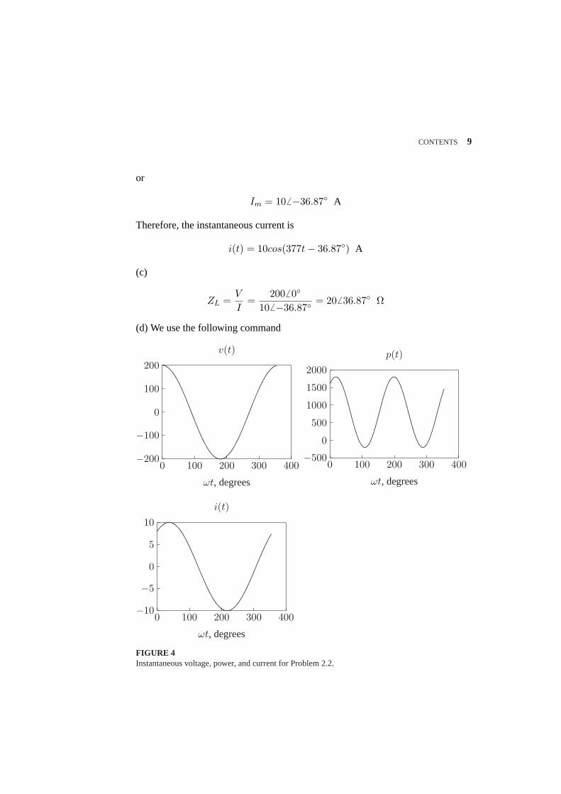
Im = 106 −36.87 A
Therefore,the instantaneous current is
i(t) = 10cos(377t− 36.87) A
(c)
ZL =V
I=
2006 0
106 −36.87= 206 36.87 Ω
(d) We use the following command
−200
−100
0
100
200
0 100 200 300 400
ωt, degrees
v(t)..............................................................................................................................................................................................................................................................................................................................................................................
..........................................................................................................................................................................................................................................................................................................................
−500
0
500
1000
1500
2000
0 100 200 300 400
ωt, degrees
p(t)
...................................................................................................................................................................................................................................................................................
...........................................................................................................................................................................................................................................................................................................................................................................................................................................................................
..........................................................................................................................................................................
−10
−5
0
5
10
0 100 200 300 400
ωt, degrees
i(t)
................................................................................................................................................................................................................................................................................................................................................................................................................
......................................................................................................................................................................................................................................................
FIGURE 4Instantaneous voltage, power, and current for Problem 2.2.

10 CONTENTS
Vm = 200;t=0:.0001:0.01667; % wt from 0 to 2*piv=Vm*cos(377*t); % Instantaneous voltagep = 800 + 1000*cos(754*t - 36.87*pi/180);% Instantaneous poweri=p./v; % Instantaneous currentwt=180/pi*377*t; % converting radian to degreexline = zeros(1, length(wt)); % generates a zero vectorsubplot(221), plot(wt, v, wt, xline), gridxlabel(’wt, degrees’), title(’v(t)’)subplot(222), plot(wt, p, wt, xline), gridxlabel(’wt, degrees’), title(’p(t)’)subplot(223), plot(wt, i, wt, xline), gridxlabel(’wt, degrees’), title(’i(t)’), subplot(111)
The result is shown in Figure 4. The inspection of current plot shows that the peakamplitude of the current is10 A, lagging voltage by36.87, with an angular fre-quency of 377 Rad/sec.
2.3.An inductive load consisting ofR andX in series feeding from a 2400-V rmssupply absorbs 288 kW at a lagging power factor of 0.8. DetermineR andX.
......................................................................
.......................................................................
.................................... ......................... ...........
.............. ......................... ............
......................................... ................
VI
R X
+ −
FIGURE 5An inductive load, withR andX in series.
θ = cos−1 0.8 = 36.87
The complex power is
S =2880.8
6 36.87 = 3606 36.87 kVA
The current given fromS = V I∗, is
I =360× 103 6 −36.87
24006 0= 1506 −36.87 A
Therefore,the series impedance is
Z = R + jX =V
I=
24006 0
1506 −36.87= 12.8 + j9.6 Ω
Therefore,R = 12.8 Ω andX = 9.6 Ω.
CONTENTS 11
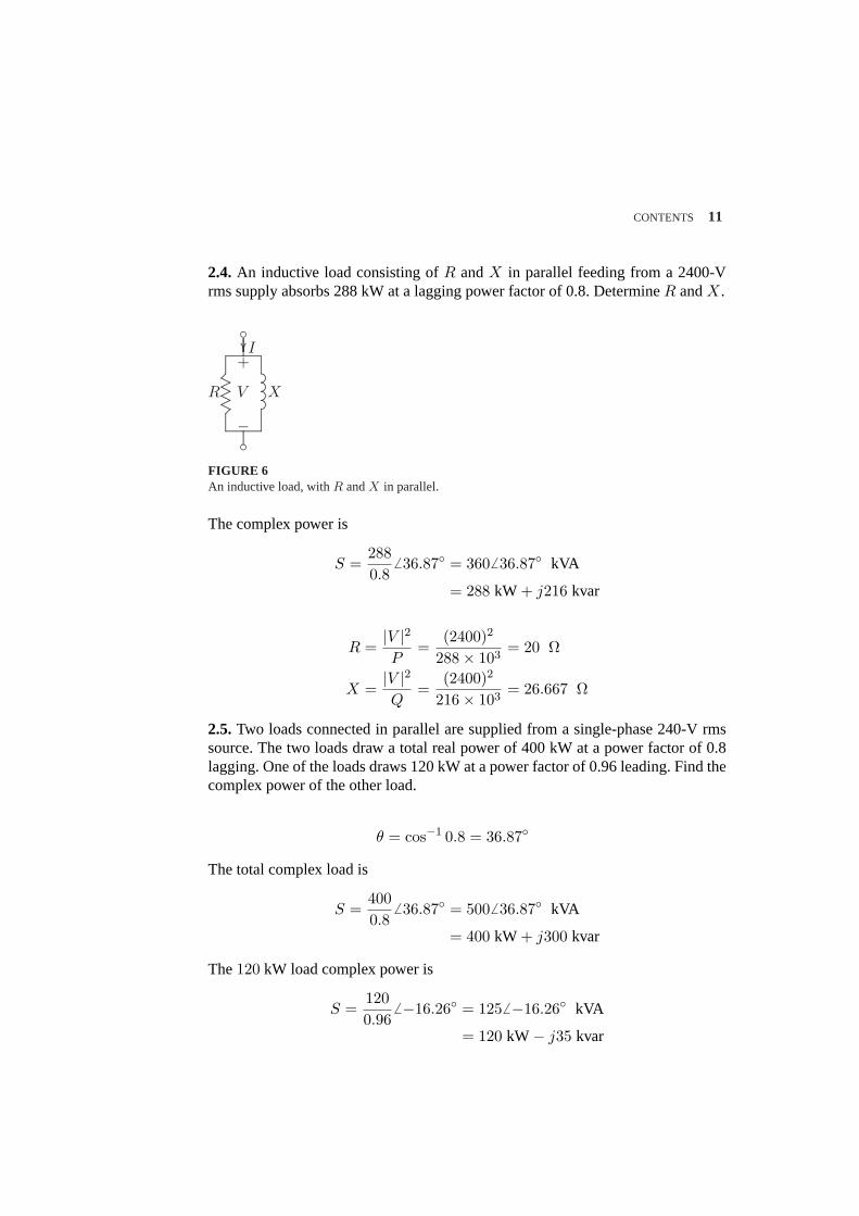
2.4. An inductive load consisting ofR andX in parallel feeding from a 2400-Vrms supply absorbs 288 kW at a lagging power factor of 0.8. DetermineR andX.
.........................................................................................................................................................................................................................................................................................................................................
..............................................................
..........................................................................................................................................................................
................................
........
........
........
V
I
R X
+
−
FIGURE 6An inductive load, withR andX in parallel.
The complex power is
S =2880.8
6 36.87 = 3606 36.87 kVA
= 288 kW + j216 kvar
R =|V |2P
=(2400)2
288× 103= 20 Ω
X =|V |2Q
=(2400)2
216× 103= 26.667 Ω
2.5.Two loads connected in parallel are supplied from a single-phase 240-V rmssource. The two loads draw a total real power of 400 kW at a power factor of 0.8lagging. One of the loads draws 120 kW at a power factor of 0.96 leading. Find thecomplex power of the other load.
θ = cos−1 0.8 = 36.87
The total complex load is
S =4000.8
6 36.87 = 5006 36.87 kVA
= 400 kW + j300 kvar
The120 kW load complex power is
S =1200.96
6 −16.26 = 1256 −16.26 kVA
= 120 kW− j35 kvar
12 CONTENTS
Therefore,the second load complex power is
S2 = 400 + j300− (120− j35) = 280 kW + j335 kvar
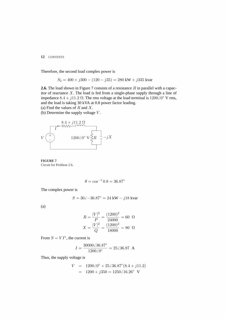
2.6.The load shown in Figure 7 consists of a resistanceR in parallel with a capac-itor of reactanceX. The load is fed from a single-phase supply through a line ofimpedance8.4 + j11.2 Ω. The rms voltage at the load terminal is12006 0 V rms,and the load is taking 30 kVA at 0.8 power factor leading.(a) Find the values ofR andX.(b) Determine the supply voltageV .
¹¸
º·......................................................................
.......................................................................
.................................... ......................... ...........
.............. ......................... ............
............. ..................................................................................................................................................................................................................................................................................................
............................ ................
V
I
8.4 + j11.2 Ω
R −jX12006 0 V+−
FIGURE 7Circuit for Problem 2.6.
θ = cos−1 0.8 = 36.87
The complex power is
S = 306 −36.87 = 24 kW− j18 kvar
(a)
R =|V |2P
=(1200)2
24000= 60 Ω
X =|V |2Q
=(1200)2
18000= 80 Ω
FromS = V I∗, the current is
I =300006 36.87
12006 0= 256 36.87 A
Thus,the supply voltage is
V = 12006 0 + 256 36.87(8.4 + j11.2)= 1200 + j350 = 12506 16.26 V
CONTENTS 13
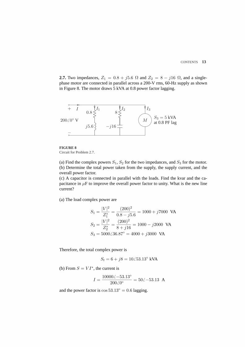
2.7. Two impedances,Z1 = 0.8 + j5.6 Ω andZ2 = 8 − j16 Ω, and a single-phase motor are connected in parallel across a 200-V rms, 60-Hz supply as shownin Figure 8. The motor draws 5 kVA at 0.8 power factor lagging.
........
........
........
............................................................................................................................................................
....................................
......................................................
........
........
........
........
........
.............................................................................
........
........
........
........
.......
........
........
........
........
........
...............................................
....................................
...............................................................
ÁÀ
¿................................ ................
........................
........
........
........ ................................................ ........................
........
........
........
I I1 I2 I3
2006 0 V
0.8
j5.6
8
−j16
S3 = 5 kVAat 0.8 PF lagM
+
−a
a
FIGURE 8Circuit for Problem 2.7.
(a) Find the complex powersS1, S2 for the two impedances, andS3 for the motor.(b) Determine the total power taken from the supply, the supply current, and theoverall power factor.(c) A capacitor is connected in parallel with the loads. Find the kvar and the ca-pacitance inµF to improve the overall power factor to unity. What is the new linecurrent?
(a) The load complex power are
S1 =|V |2Z∗1
=(200)2
0.8− j5.6= 1000 + j7000 VA
S2 =|V |2Z∗2
=(200)2
8 + j16= 1000− j2000 VA
S3 = 50006 36.87 = 4000 + j3000 VA
Therefore, the total complex power is
St = 6 + j8 = 106 53.13 kVA
(b) FromS = V I∗, the current is
I =100006 −53.13
2006 0= 506 −53.13 A
andthe power factor iscos 53.13 = 0.6 lagging.

14 CONTENTS
(c) For overall unity power factor,QC = 8000 Var, and the capacitive impedanceis
ZC =|V |2SC
∗ =(200)2
j8000= −j5 Ω
and the capacitance is
C =106
(2π)(60)(5)= 530.5 µF
The new current is
I =60006 0
2006 0= 306 0 A
2.8.Two single-phase ideal voltage sources are connected by a line of impedance of0.7 + j2.4 Ω as shown in Figure 9.V1 = 5006 16.26 V andV2 = 5856 0 V. Findthe complex power for each machine and determine whether they are delivering orreceiving real and reactive power. Also, find the real and the reactive power loss inthe line.
¹¸
º·......................................................................
.......................................................................
.................................... ......................... ...........
.............. ......................... ...........
..............
¹¸
º·............................ ................
5006 16.26 V
I12
0.7 + j2.4 Ω
5856 0 V+−
+−
FIGURE 9Circuit for Problem 2.8.
I12 =5006 16.26 − 5856 0
0.7 + j2.4= 42 + j56 = 706 53.13 A
S12 = V1I∗12 = (5006 16.26)(706 −53.13) = 350006 −36.87
= 28000− j21000 VA
S21 = V2I∗21 = (5856 0)(−706 −53.13) = 409506 −53.13
= −24570 + j32760 VA

CONTENTS 15
Fromthe above results, sinceP1 is positive andP2 is negative, source 1 generates28 kW, and source 2 receives24.57 kW, and the real power loss is3.43 kW. Sim-ilarly, sinceQ1 is negative, source 1 receives21 kvar and source 2 delivers32.76kvar. The reactive power loss in the line is11.76 kvar.
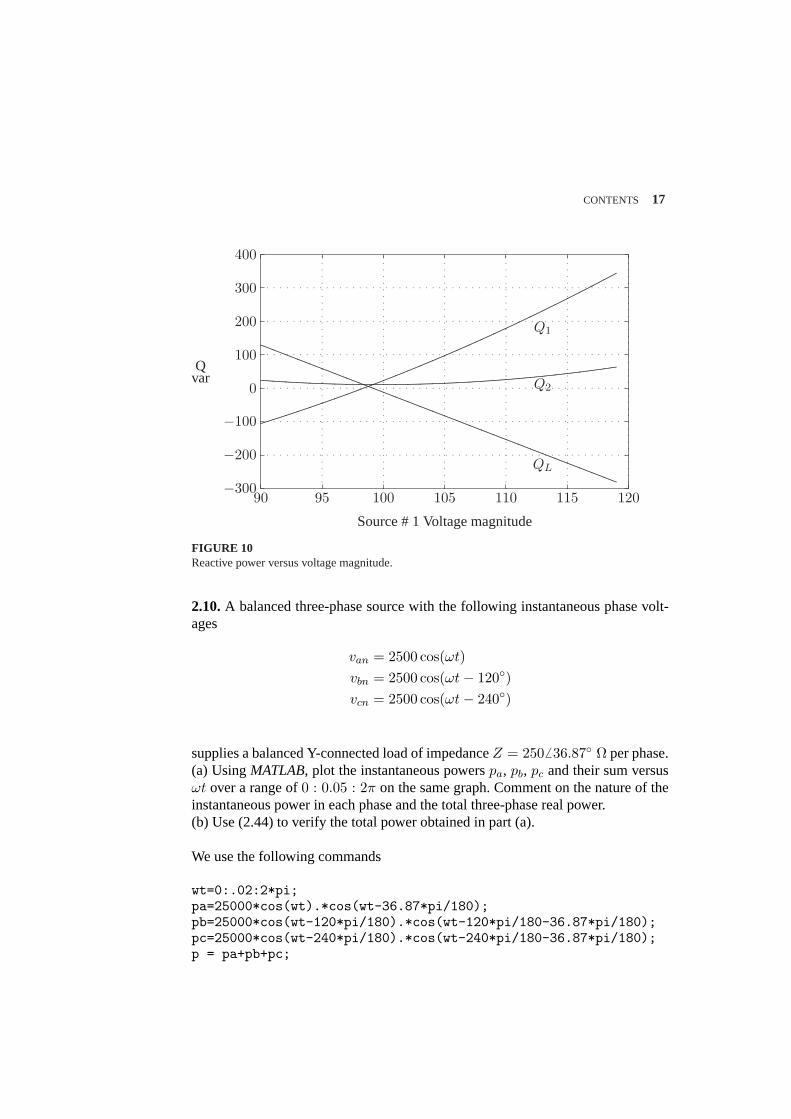
2.9.Write aMATLABprogram for the system of Example 2.5 such that the voltagemagnitude of source 1 is changed from 75 percent to 100 percent of the given valuein steps of 1 volt. The voltage magnitude of source 2 and the phase angles of thetwo sources is to be kept constant. Compute the complex power for each source andthe line loss. Tabulate the reactive powers and plotQ1, Q2, andQL versus voltagemagnitude|V1|. From the results, show that the flow of reactive power along theinterconnection is determined by the magnitude difference of the terminal voltages.
We use the following commands
E1 = input(’Source # 1 Voltage Mag. = ’);a1 = input(’Source # 1 Phase Angle = ’);E2 = input(’Source # 2 Voltage Mag. = ’);a2 = input(’Source # 2 Phase Angle = ’);R = input(’Line Resistance = ’);X = input(’Line Reactance = ’);Z = R + j*X; % Line impedanceE1 = (0.75*E1:1:E1)’; % Change E1 form 75% to 100% E1a1r = a1*pi/180; % Convert degree to radiank = length(E1);E2 = ones(k,1)*E2;%create col. Array of same length for E2a2r = a2*pi/180; % Convert degree to radianV1=E1.*cos(a1r) + j*E1.*sin(a1r);V2=E2.*cos(a2r) + j*E2.*sin(a2r);I12 = (V1 - V2)./Z; I21=-I12;S1= V1.*conj(I12); P1 = real(S1); Q1 = imag(S1);S2= V2.*conj(I21); P2 = real(S2); Q2 = imag(S2);SL= S1+S2; PL = real(SL); QL = imag(SL);Result1=[E1, Q1, Q2, QL];disp(’ E1 Q-1 Q-2 Q-L ’)disp(Result1)plot(E1, Q1, E1, Q2, E1, QL), gridxlabel(’ Source #1 Voltage Magnitude’)ylabel(’ Q, var’)text(112.5, -180, ’Q2’)text(112.5, 5,’QL’), text(112.5, 197, ’Q1’)
The result is

16 CONTENTS
Source # 1 Voltage Mag. = 120Source # 1 Phase Angle = -5Source # 2 Voltage Mag. = 100Source # 2 Phase Angle = 0Line Resistance = 1Line Reactance = 7
E1 Q-1 Q-2 Q-L
90.0000 -105.5173 129.1066 23.589491.0000 -93.9497 114.9856 21.035992.0000 -82.1021 100.8646 18.762593.0000 -69.9745 86.7435 16.769094.0000 -57.5669 72.6225 15.055695.0000 -44.8794 58.5015 13.622196.0000 -31.9118 44.3804 12.468797.0000 -18.6642 30.2594 11.595298.0000 -5.1366 16.1383 11.001799.0000 8.6710 2.0173 10.6883100.0000 22.7586 -12.1037 10.6548101.0000 37.1262 -26.2248 10.9014102.0000 51.7737 -40.3458 11.4279103.0000 66.7013 -54.4668 12.2345104.0000 81.9089 -68.5879 13.3210105.0000 97.3965 -82.7089 14.6876106.0000 113.1641 -96.8299 16.3341107.0000 129.2117 -110.9510 18.2607108.0000 145.5393 -125.0720 20.4672109.0000 162.1468 -139.1931 22.9538110.0000 179.0344 -153.3141 25.7203111.0000 196.2020 -167.4351 28.7669112.0000 213.6496 -181.5562 32.0934113.0000 231.3772 -195.6772 35.7000114.0000 249.3848 -209.7982 39.5865115.0000 267.6724 -223.9193 43.7531116.0000 286.2399 -238.0403 48.1996117.0000 305.0875 -252.1614 52.9262118.0000 324.2151 -266.2824 57.9327119.0000 343.6227 -280.4034 63.2193120.0000 363.3103 -294.5245 68.7858
Examination of Figure 10 shows that the flow of reactive power along the intercon-nection is determined by the voltage magnitude difference of terminal voltages.
CONTENTS 17
−300
−200
−100
0
100
200
300
400
Qvar
90 95 100 105 110 115 120
Source # 1 Voltage magnitude
.....................................................
..................................................
................................................
.............................................
............................................
...........................................
.........................................
..........................................
..........................................
.......................................
.......................................
.....................................
......................................
...................................
...................................
....................................
...................................
...................................
.......
.....................................................................................................................................................................................................................................................................................................................................................................................................................................................................................................................................................................................................................................................................................................................................................
.................................................................................................................................................................................................................................................................................................................................................................................................................................................................................................................................................................
....................................................................................................................................
...................
Q1
Q2
QL
.
.
.
.
.
.
.
.
.
.
.
.
.
.
.
.
.
.
.
.
.
.
.
.
.
.
.
.
.
.
.
.
.
.
.
.
.
.
.
.
.
.
.
.
.
.
.
.
.
.
.
.
.
.
.
.
.
.
.
.
.
.
.
.
.
.
.
.
.
.
.
.
.
.
.
.
.
.
.
.
.
.
.
.
.
.
.
.
.
.
.
.
.
.
.
.
.
.
.
.
.
.
.
.
.
.
.
.
.
.
.
.
.
.
.
.
.
.
.
.
.
.
.
.
.
.
.
.
.
.
.
.
.
.
.
.
.
.
.
.
.
.
.
.
.
.
.
.
.
.
.
.
.
.
.
.
.
.
.
.
.
.
.
.
.
.
.
.
.
.
.
.
.
.
.
.
.
.
.
.
.
.
.
.
.
.
.
.
.
.
.
.
.
.
.
.
.
.
.
.
.
.
.
.
.
.
.
.
.
.
.
.
.
.
.
.
. . . . . . . . . . . . . . . . . . . . . . . . . . . . . . . . . . . . . . . . . . . . . . . . . . . . . . . .
. . . . . . . . . . . . . . . . . . . . . . . . . . . . . . . . . . . . . . . . . . . . . . . . . . . . . . . .
. . . . . . . . . . . . . . . . . . . . . . . . . . . . . . . . . . . . . . . . . . . . . . . . . . . . . . . .
. . . . . . . . . . . . . . . . . . . . . . . . . . . . . . . . . . . . . . . . . . . . . . . . . . . . . . . .
. . . . . . . . . . . . . . . . . . . . . . . . . . . . . . . . . . . . . . . . . . . . . . . . . . . . . . . .
. . . . . . . . . . . . . . . . . . . . . . . . . . . . . . . . . . . . . . . . . . . . . . . . . . . . . . . .
FIGURE 10Reactive power versus voltage magnitude.
2.10.A balanced three-phase source with the following instantaneous phase volt-ages
van = 2500 cos(ωt)vbn = 2500 cos(ωt− 120)vcn = 2500 cos(ωt− 240)
supplies a balanced Y-connected load of impedanceZ = 2506 36.87 Ω perphase.(a) UsingMATLAB, plot the instantaneous powerspa, pb, pc and their sum versusωt over a range of0 : 0.05 : 2π on the same graph. Comment on the nature of theinstantaneous power in each phase and the total three-phase real power.(b) Use (2.44) to verify the total power obtained in part (a).
We use the following commands
wt=0:.02:2*pi;pa=25000*cos(wt).*cos(wt-36.87*pi/180);pb=25000*cos(wt-120*pi/180).*cos(wt-120*pi/180-36.87*pi/180);pc=25000*cos(wt-240*pi/180).*cos(wt-240*pi/180-36.87*pi/180);p = pa+pb+pc;

18 CONTENTS
plot(wt, pa, wt, pb, wt, pc, wt, p), gridxlabel(’Radian’)disp(’(b)’)V = 2500/sqrt(2);gama = acos(0.8);Z = 250*(cos(gama)+j*sin(gama));I = V/Z;P = 3*V*abs(I)*0.8
−0.5
0
0.5
1
1.5
2
2.5
3
0 1 2 3 4 5 6 7 8
Radian
...........................................................................................................................................................................................................................................................................................................................................................................................................
..........................................................................................................................................................................................................................................................................................................................................................................................................................................................................................................................................................................................................................................................................................
....................................................................................................................................................................................................................................................................
...............................................................................................................................................................................................................................................................................................................................................................................................................................................................................................................................
..........................................................................................................................................................................................................................................................................................................................................................................................................................................................................................................................................................................................................................................................................................................................................................................................................................................
..................................................................................................................................................................................................................................................................................................................................................................................................................................................................................................................................................................................................................................................................................
..........................................................................................................................................................................................................................................................................................................................................................................................................................................................................................................................................................................................................................................................................................
........................................................................................................................................................................................................................................................................................................................................................................................................................................................................................................................................................................................×104
.
.
.
.
.
.
.
.
.
.
.
.
.
.
.
.
.
.
.
.
.
.
.
.
.
.
.
.
.
.
.
.
.
.
.
.
.
.
.
.
.
.
.
.
.
.
.
.
.
.
.
.
.
.
.
.
.
.
.
.
.
.
.
.
.
.
.
.
.
.
.
.
.
.
.
.
.
.
.
.
.
.
.
.
.
.
.
.
.
.
.
.
.
.
.
.
.
.
.
.
.
.
.
.
.
.
.
.
.
.
.
.
.
.
.
.
.
.
.
.
.
.
.
.
.
.
.
.
.
.
.
.
.
.
.
.
.
.
.
.
.
.
.
.
.
.
.
.
.
.
.
.
.
.
.
.
.
.
.
.
.
.
.
.
.
.
.
.
.
.
.
.
.
.
.
.
.
.
.
.
.
.
.
.
.
.
.
.
.
.
.
.
.
.
.
.
.
.
.
.
.
.
.
.
.
.
.
.
.
.
.
.
.
.
.
.
.
. . . . . . . . . . . . . . . . . . . . . . . . . . . . . . . . . . . . . . . . . . . . . . . . . . . . . . . . . .
. . . . . . . . . . . . . . . . . . . . . . . . . . . . . . . . . . . . . . . . . . . . . . . . . . . . . . . . . .
. . . . . . . . . . . . . . . . . . . . . . . . . . . . . . . . . . . . . . . . . . . . . . . . . . . . . . . . . .
. . . . . . . . . . . . . . . . . . . . . . . . . . . . . . . . . . . . . . . . . . . . . . . . . . . . . . . . . .
. . . . . . . . . . . . . . . . . . . . . . . . . . . . . . . . . . . . . . . . . . . . . . . . . . . . . . . . . .
. . . . . . . . . . . . . . . . . . . . . . . . . . . . . . . . . . . . . . . . . . . . . . . . . . . . . . . . . .
. . . . . . . . . . . . . . . . . . . . . . . . . . . . . . . . . . . . . . . . . . . . . . . . . . . . . . . . . .
FIGURE 11Instantaneous powers and their sum for Problem 2.10.
(b)
V =2500√
2= 1767.776 0 V
I =1767.776 0
2506 36.87= 7.0716 −36.87 A
P = (3)(1767.77)(7.071)(0.8) = 30000 W
2.11.A 4157-V rms three-phase supply is applied to a balanced Y-connected three-phase load consisting of three identical impedances of486 36.87 Ω. Taking thephase to neutral voltageVan as reference, calculate(a) The phasor currents in each line.(b) The total active and reactive power supplied to the load.
Van =4157√
3= 2400 V

CONTENTS 19
With Van as reference, the phase voltages are:
Van = 24006 0 V Vbn = 24006 −120 V Van = 24006 −240 V
(a)The phasor currents are:
Ia =Van
Z=
24006 0
486 36.87= 506 −36.87 A
Ib =Vbn
Z=
24006 −120
486 36.87= 506 −156.87 A
Ic =Vcn
Z=
24006 −240
486 36.87= 506 −276.87 A
(b) The total complex power is
S = 3VanI∗a = (3)(24006 0)(506 36.87) = 3606 36.87 kVA
= 288 kW + j216 KVAR
2.12.Repeat Problem 2.11 with the same three-phase impedances arranged in a∆connection. TakeVab as reference.
Van =4157√
3= 2400 V
With Vab as reference, the phase voltages are:
Iab =Vab
Z=
41576 0
486 36.87= 86.66 −36.87 A
Ia =√
36 −30Iab = (√
36 −30)(86.66 −36.87 = 1506 −66.87 A
For positive phase sequence, current in other lines are
Ib = 1506 −186.87 A, andIc = 1506 53.13 A
(b) The total complex power is
S = 3VabI∗ab = (3)(41576 0)(86.6 6 36.87) = 10806 36.87 kVA
= 864 kW + j648 kvar
2.13.A balanced delta connected load of15 + j18 Ω per phase is connected at theend of a three-phase line as shown in Figure 12. The line impedance is1+j2 Ω perphase. The line is supplied from a three-phase source with a line-to-line voltage of207.85 V rms. TakingVan as reference, determine the following:

20 CONTENTS
...................................................................................................................................................................................................
.......................................................................
................. ......................... ...........
.............. ......................... ...........
.............. ..................................................................................................................................................................................................................................................................................................................................................................
...................................................................................................................................................................................................
.......................................................................
................. ......................... ...........
.............. ......................... ...........
.............. ..................................................................................................................................................................................................
...................................................................................................................................................................................................
.......................................................................
................. ......................... ...........
.............. ......................... ...........
.............. ..................................................................................................................................................................................................................................................................................................................................................................
...........................................................................................................................................................................
.......................
.........................
.........................
..
........
........
........
.......
................................
..................................................
........
................................................................
.................
.........................................................................
..............................
.
.............................................................................................
..............................................................................
........
.................................................
................................................
1 + j2 Ω
15 + j18 Ω
|VL| = 207.85 V
b
b
b
a
b
c
a
b
c
FIGURE 12Circuit for Problem 2.13.
(a) Current in phasea.(b) Total complex power supplied from the source.(c) Magnitude of the line-to-line voltage at the load terminal.
Van =207.85√
3= 120 V
Transforming the delta connected load to an equivalent Y-connected load, result inthe phase ’a’ equivalent circuit, shown in Figure 13.
...................................................................................................................................................................................................
.......................................................................
................. ......................... ...........
.............. ......................... ...........
.............. .........................................................................................................................................................................
........
........
........
.......
.........................
.........................
.........................
........
.........
..........................................................................................................................................................
...............................................................................................................................................................................................................................................................................................................................................................................................................................................
1 + j2 Ω
5 Ω
j6 ΩV1 = 1206 0 V V2
+
−
b
b
a
n
................................ ................Ia
FIGURE 13The per phase equivalent circuit for Problem 2.13.
(a)
Ia =1206 0
6 + j8= 12 6 −53.13 A
(b) The total complex power is
S = 3VanI∗a = (3)(1206 0)(126 53.13 = 43206 53.13 VA
= 2592 W + j3456 Var
(c)
V2 = 1206 0 − (1 + j2)(126 −53.13 = 93.726 −2.93 A
CONTENTS 21
Thus,the magnitude of the line-to-line voltage at the load terminal isVL =√
3(93.72) =162.3 V.
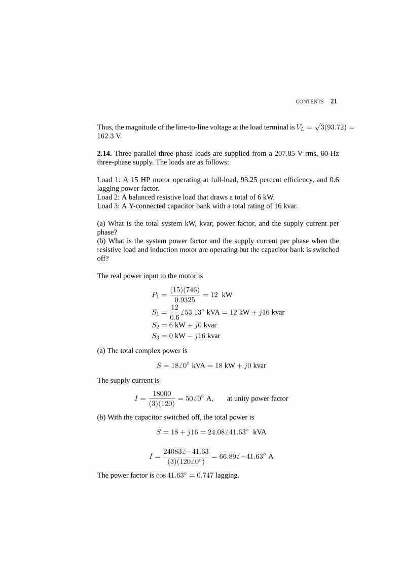
2.14.Three parallel three-phase loads are supplied from a 207.85-V rms, 60-Hzthree-phase supply. The loads are as follows:
Load 1: A 15 HP motor operating at full-load, 93.25 percent efficiency, and 0.6lagging power factor.Load 2: A balanced resistive load that draws a total of 6 kW.Load 3: A Y-connected capacitor bank with a total rating of 16 kvar.
(a) What is the total system kW, kvar, power factor, and the supply current perphase?(b) What is the system power factor and the supply current per phase when theresistive load and induction motor are operating but the capacitor bank is switchedoff?
The real power input to the motor is
P1 =(15)(746)0.9325
= 12 kW
S1 =120.6
6 53.13 kVA = 12 kW + j16 kvar
S2 = 6 kW + j0 kvar
S3 = 0 kW− j16 kvar
(a) The total complex power is
S = 18 6 0 kVA = 18 kW + j0 kvar
The supply current is
I =18000
(3)(120)= 506 0 A, atunity power factor
(b) With the capacitor switched off, the total power is
S = 18 + j16 = 24.086 41.63 kVA
I =240836 −41.63(3)(1206 0)
= 66.896 −41.63 A
Thepower factor iscos 41.63 = 0.747 lagging.
22 CONTENTS
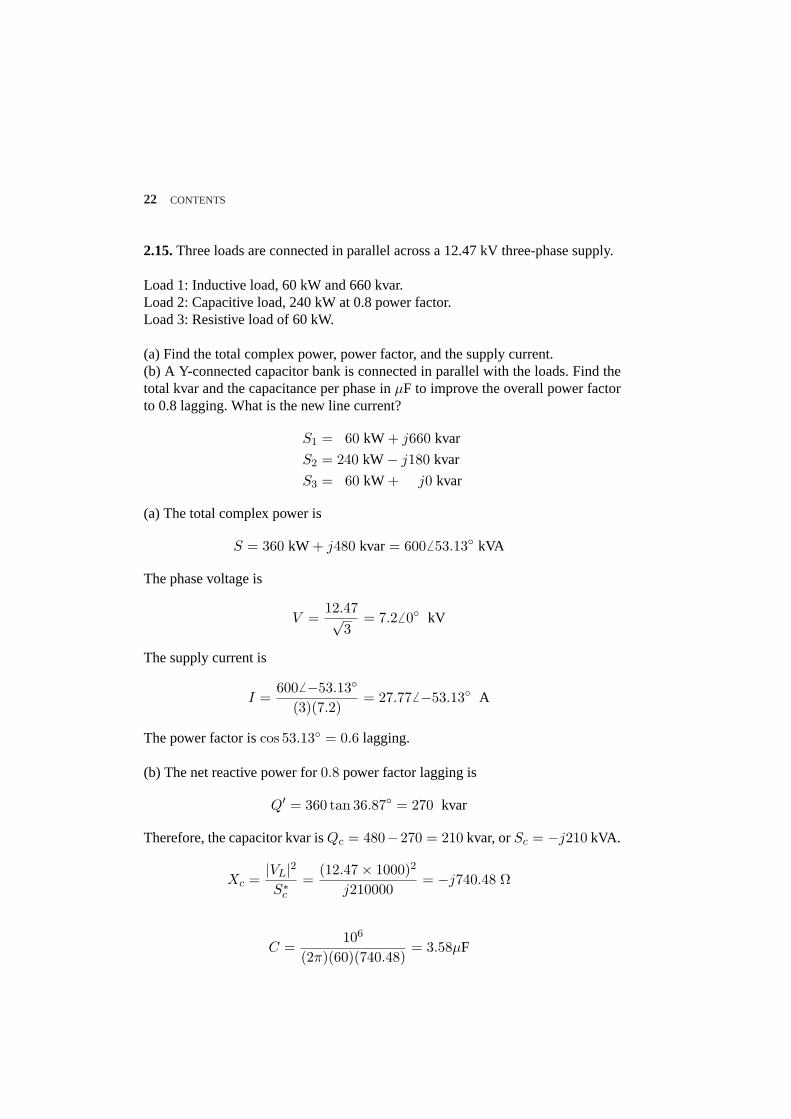
2.15.Threeloads are connected in parallel across a 12.47 kV three-phase supply.
Load 1: Inductive load, 60 kW and 660 kvar.Load 2: Capacitive load, 240 kW at 0.8 power factor.Load 3: Resistive load of 60 kW.
(a) Find the total complex power, power factor, and the supply current.(b) A Y-connected capacitor bank is connected in parallel with the loads. Find thetotal kvar and the capacitance per phase inµF to improve the overall power factorto 0.8 lagging. What is the new line current?
S1 = 60 kW + j660 kvar
S2 = 240 kW− j180 kvar
S3 = 60 kW + j0 kvar
(a) The total complex power is
S = 360 kW + j480 kvar = 6006 53.13 kVA
The phase voltage is
V =12.47√
3= 7.26 0 kV
Thesupply current is
I =6006 −53.13
(3)(7.2)= 27.776 −53.13 A
Thepower factor iscos 53.13 = 0.6 lagging.
(b) The net reactive power for0.8 power factor lagging is
Q′ = 360 tan 36.87 = 270 kvar
Therefore, the capacitor kvar isQc = 480−270 = 210 kvar, orSc = −j210 kVA.
Xc =|VL|2S∗c
=(12.47× 1000)2
j210000= −j740.48 Ω
C =106
(2π)(60)(740.48)= 3.58µF

CONTENTS 23
.................................................................................................................................... ................................................................................................................................................................................................................................................
................................................................................................................................................................................
............................................................................
........
........
........
........
........
........
........
........
........
........
........
........
........
.......................
................
........
........
........
........
........
........
........
........
....................
................ Q
Q′
P
Qc
θ′ ........................................
FIGURE 14The power diagram for Problem 2.15.
I =S∗
V ∗ =360− j270
(3)(7.2)= 20.8356 −36.87 A
2.16.A balanced∆-connected load consisting of a pure resistances of18 Ω perphase is in parallel with a purely resistive balanced Y-connected load of12 Ωper phase as shown in Figure 15. The combination is connected to a three-phasebalanced supply of 346.41-V rms (line-to-line) via a three-phase line having aninductive reactance ofj3 Ω per phase. Taking the phase voltageVan as reference,determine(a) The current, real power, and reactive power drawn from the supply.(b) The line-to-neutral and the line-to-line voltage of phasea at the combined loadterminals.
....................................
..................................................
..............
....................................
..................................................
..............
....................................
..................................................
..............
.........................................................................................................................................................................................
............................................................................................................................................................................................................................................................................................................
................................................................................................................................................................................................................
........................................................................................................................................................................................................................................................
................................
..................................................
........
................................................................
...............................
.................................
..............................
..........................................................................................................................................................................
..............................................................................
...................................................
........
................................................................
.................................
................................
............................................................................................................................................
....................................
.......................................
..........................................................................................................................................................
...............................................
j3 Ω
18 Ω
12 Ω
n
|VL| = 346.41 V
b
b
b
a
b
c
a
a
a
a
b
c
FIGURE 15Circuit for Problem 2.16.

24 CONTENTS
Transforming the delta connected load to an equivalent Y-connected load, result inthe phase ’a’ equivalent circuit, shown in Figure 16.
........................................................................................................................................................................................................ ......................... ...........
.............. ......................... ...........
.............. ...........................................................................................................................................................................................................................................................................................................................................................................................................................................................................................................................................................................................
........
........
........
.......
........
.........
..........................................................................................................................................................
.......................................................................................................................................................................................................................................................................................................................................................................................................................................................................................................................................................................................................................................
j3 Ω
6 Ω12 ΩV1 = 2006 0 V V2
+
−
b
b
a
n
................................ ................
........................
........
........
........ ................................................
I
I1 I2
FIGURE 16The per phase equivalent circuit for Problem 2.16.
(a)
Van =346.41√
3= 200 V
The input impedance is
Z =(12)(6)12 + 6
+ j3 = 4 + j3 Ω
Ia =2006 0
4 + j3= 40 6 −36.87 A
Thetotal complex power is
S = 3VanI∗a = (3)(2006 0)(406 36.87) = 240006 36.87 VA
= 19200 W + j14400 Var
(b)
V2 = 2006 0 − (j3)(406 −36.87) = 1606 −36.87 A
Thus,the magnitude of the line-to-line voltage at the load terminal isVL =√
3(160) =277.1 V.

CHAPTER3 PROBLEMS
3.1. A three-phase, 318.75-kVA, 2300-V alternator has an armature resistance of0.35Ω/phase and a synchronous reactance of 1.2Ω/phase. Determine the no-loadline-to-line generated voltage and the voltage regulation at(a) Full-load kVA, 0.8 power factor lagging, and rated voltage.(b) Full-load kVA, 0.6 power factor leading, and rated voltage.
Vφ =2300√
3= 1327.9 V
(a) For318.75 kVA, 0.8 power factor lagging,S = 3187506 36.87 VA.
Ia =S∗
3V ∗φ
=3187506 −36.87
(3)(1327.9)= 806 −36.87 A
Eφ = 1327.9 + (0.35 + j1.2)(806 −36.87) = 1409.26 2.44 V
Themagnitude of the no-load generated voltage isELL =
√3 1409.2 = 2440.8 V, and the voltage regulation is
V.R. =2440.8− 2300
2300× 100 = 6.12%
(b) For318.75 kVA, 0.6 power factor leading,S = 3187506 −53.13 VA.
Ia =S∗
3V ∗φ
=3187506 53.13
(3)(1327.9= 806 53.13 A
25

26 CONTENTS
Eφ = 1327.9 + (0.35 + j1.2)(806 53.13) = 1270.46 3.61 V
Themagnitude of the no-load generated voltage isELL =
√3 1270.4 = 2220.4 V, and the voltage regulation is
V.R. =2200.4− 2300
2300× 100 = −4.33%
3.2. A 60-MVA, 69.3-kV, three-phase synchronous generator has a synchronousreactance of 15Ω/phase and negligible armature resistance.
(a) The generator is delivering rated power at 0.8 power factor lagging at the ratedterminal voltage to an infinite bus bar. Determine the magnitude of the generatedemf per phase and the power angleδ.
(b) If the generated emf is 36 kV per phase, what is the maximum three-phasepower that the generator can deliver before losing its synchronism?
(c) The generator is delivering 48 MW to the bus bar at the rated voltage withits field current adjusted for a generated emf of 46 kV per phase. Determine thearmature current and the power factor. State whether power factor is lagging orleading?
Vφ =69.3√
3= 40 kV
(a) For60 kVA, 0.8 power factor lagging,S = 600006 36.87 kVA.
Ia =S∗
3V ∗φ
=600006 −36.87
(3)(40)= 5006 −36.87 A
Eφ = 40 + (j15)(5006 −36.87)× 10−3 = 44.96 7.675 kV
(b)
Pmax =3|E||V |
Xs=
(3)(36)(40)15
= 288 MW
(c) ForP = 48 MW, andE = 46 KV/phase, the power angle is given by
48 =(3)(46)(40)
15sin δ
CONTENTS 27
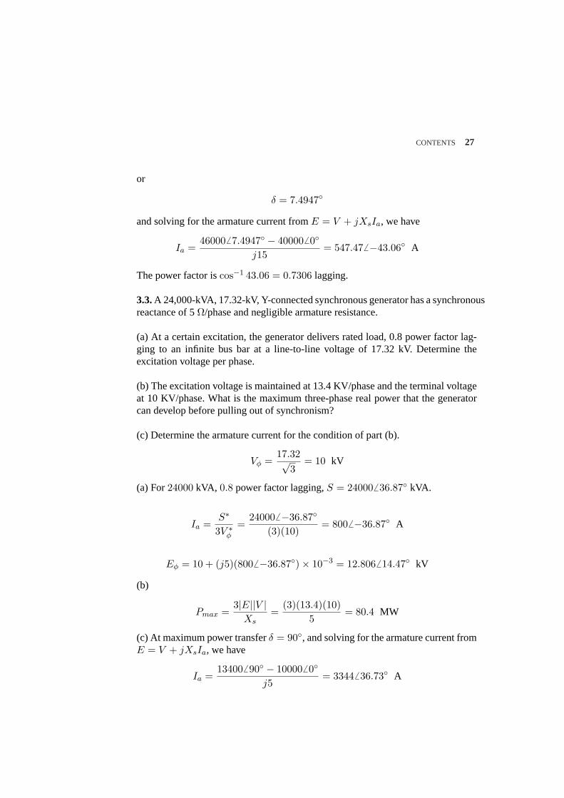
or
δ = 7.4947
and solving for the armature current fromE = V + jXsIa, we have
Ia =460006 7.4947 − 400006 0
j15= 547.476 −43.06 A
Thepower factor iscos−1 43.06 = 0.7306 lagging.
3.3.A 24,000-kVA, 17.32-kV, Y-connected synchronous generator has a synchronousreactance of 5Ω/phase and negligible armature resistance.
(a) At a certain excitation, the generator delivers rated load, 0.8 power factor lag-ging to an infinite bus bar at a line-to-line voltage of 17.32 kV. Determine theexcitation voltage per phase.
(b) The excitation voltage is maintained at 13.4 KV/phase and the terminal voltageat 10 KV/phase. What is the maximum three-phase real power that the generatorcan develop before pulling out of synchronism?
(c) Determine the armature current for the condition of part (b).
Vφ =17.32√
3= 10 kV
(a) For24000 kVA, 0.8 power factor lagging,S = 240006 36.87 kVA.
Ia =S∗
3V ∗φ
=240006 −36.87
(3)(10)= 8006 −36.87 A
Eφ = 10 + (j5)(8006 −36.87)× 10−3 = 12.8066 14.47 kV
(b)
Pmax =3|E||V |
Xs=
(3)(13.4)(10)5
= 80.4 MW
(c) At maximum power transferδ = 90, and solving for the armature current fromE = V + jXsIa, we have
Ia =134006 90 − 100006 0
j5= 33446 36.73 A

28 CONTENTS
Thepower factor iscos−1 36.73 = 0.7306 leading.
3.4. A 34.64-kV, 60-MVA, three-phase salient-pole synchronous generator has adirect axis reactance of 13.5Ω and a quadrature-axis reactance of 9.333Ω. Thearmature resistance is negligible.
(a) Referring to the phasor diagram of a salient-pole generator shown in Figure 17,show that the power angleδ is given by
δ = tan−1
(Xq|Ia| cos θ
V + Xq|Ia| sin θ
)
(b) Compute the load angleδ and the per phase excitation voltageE when thegenerator delivers rated MVA, 0.8 power factor lagging to an infinite bus bar of34.64-kV line-to-line voltage.
(c) The generator excitation voltage is kept constant at the value found in part (b).UseMATLABto obtain a plot of the power angle curve, i.e., equation (3.26) over arange ofd = 0 : .05 : 180. Use the command [Pmax, k] = max(P);dmax = d(k),to obtain the steady-state maximum powerPmax and the corresponding power an-gledmax.
......................................................................................................................................................................................................................................................................................................................................................................................................................................................................................................................................................... ........................................................................................................................................................................................................................................................................................................................................................................... ......................................................................................................................................................................................................................................................... ................ ........
........
........
........
........
........
........
........
........
........
........
........
........
........
........
........
...................
...................................................................................................................................................................................................................................................................................... ..........
......
.............................................................................................................................................................................................. ......................................................................................................................................................................................................
........
........
........
E
XdId
jXqIq
Ia
V
Id
Iq da
bc
e
δ
..........................................δ
....................................
θ
............. ............. ............. ............. ............. ............. ............. ........................................................................................................
..........................
............. ............. ..........................
..........................
..........................
................
FIGURE 17Phasor diagram of a salient-pole generator for Problem 3.4.
(a) Form the phasor diagram shown in Figure 17, we have
|V | sin δ = XqIq
= Xq|Ia| cos(θ + δ)= Xq|Ia|(cos θ cos δ − sin θ sin δ)
or
sin δ
cos δ=
Xq|Ia| cos θ
V + Xq|Ia| sin θ

CONTENTS 29
or
δ = tan−1 Xq|Ia| cos θ
V + Xq|Ia| sin θ
(b)
Vφ =34.64√
3= 20 kV
(a) For60 MVA, 0.8 power factor lagging,S = 60 6 36.87 MVA
Ia =S∗
3V ∗φ
=600006 −36.87
(3)(20)= 10006 −36.87 A
δ = tan−1 (9.333)(1000)(0.8)20000 + (9.333)(1000)(0.6)
= 16.26
The magnitude of the no-load generated emf per phase is given by
|E| = |V | cos δ + Xd|Ia| sin(θ + δ)= 20 cos 16.26 + (13.5)(1000)(10−3) sin 53.13 = 30 kV
(c) We use the following commands
V = 20000; Xd = 13.5; Xq = 9.333;theta=acos(0.8);Ia = 20E06/20000;delta = atan(Xq*Ia*cos(theta)/(V + Xq*Ia*sin(theta)));deltadg=delta*180/pi;E = V*cos(delta)+Xd*Ia*sin(theta+delta);E_KV = E/1000; % Excitaiton voltage in kVfprintf(’Power angle = %g Degree \n’, deltadg)fprintf(’E = %g kV \n\n’, E_KV)deltadg = (0:.25:180)’;delta=deltadg*pi/180;P=3*E*V/Xd*sin(delta)+3*V^2*(Xd-Xq)/(2*Xd*Xq)*sin(2*delta);P = P/1000000; % Power in MWplot(deltadg, P), gridxlabel(’Delta - Degree’), ylabel(’P - MW’)[Pmax, k]=max(P); delmax=deltadg(k);fprintf(’Max power = %g MW’,Pmax)fprintf(’ at power angle %g degree \n’, delmax)

30 CONTENTS
0
20
40
60
80
100
120
140
PMW
0 20 40 60 80 100 120 140 160 180
Delta, degree
..................................................................................................................................................................................................................................................................................................................................................................................................................................................................................................................................................................................................
........................................................................................
......................................................................................................................................................................................................................................................................................................................................................................................................................................................................................................................................................................................................................................................................................................................................................................................................................................................................................................................................
.
.
.
.
.
.
.
.
.
.
.
.
.
.
.
.
.
.
.
.
.
.
.
.
.
.
.
.
.
.
.
.
.
.
.
.
.
.
.
.
.
.
.
.
.
.
.
.
.
.
.
.
.
.
.
.
.
.
.
.
.
.
.
.
.
.
.
.
.
.
.
.
.
.
.
.
.
.
.
.
.
.
.
.
.
.
.
.
.
.
.
.
.
.
.
.
.
.
.
.
.
.
.
.
.
.
.
.
.
.
.
.
.
.
.
.
.
.
.
.
.
.
.
.
.
.
.
.
.
.
.
.
.
.
.
.
.
.
.
.
.
.
.
.
.
.
.
.
.
.
.
.
.
.
.
.
.
.
.
.
.
.
.
.
.
.
.
.
.
.
.
.
.
.
.
.
.
.
.
.
.
.
.
.
.
.
.
.
.
.
.
.
.
.
.
.
.
.
.
.
.
.
.
.
.
.
.
.
.
.
.
.
.
.
.
.
.
. . . . . . . . . . . . . . . . . . . . . . . . . . . . . . . . . . . . . . . . . . . . . . . . . . . . . . . . . .
. . . . . . . . . . . . . . . . . . . . . . . . . . . . . . . . . . . . . . . . . . . . . . . . . . . . . . . . . .
. . . . . . . . . . . . . . . . . . . . . . . . . . . . . . . . . . . . . . . . . . . . . . . . . . . . . . . . . .
. . . . . . . . . . . . . . . . . . . . . . . . . . . . . . . . . . . . . . . . . . . . . . . . . . . . . . . . . .
. . . . . . . . . . . . . . . . . . . . . . . . . . . . . . . . . . . . . . . . . . . . . . . . . . . . . . . . . .
. . . . . . . . . . . . . . . . . . . . . . . . . . . . . . . . . . . . . . . . . . . . . . . . . . . . . . . . . .
FIGURE 18Power angle curve for Problem 3.4.
The result is
Power angle = 16.2598 DegreeE = 30 kVMax power = 138.712 MW at power angle 75 degree
3.5.A 150-kVA, 2400/240-V single-phase transformer has the parameters as shownin Figure 19.
......................................................................................................................................
.......................................................................
................. ......................... ...........
.............. ......................... ...........
.............. ..............................................................................................................................................................................................................................................................................
...........................................................................................................................................................................................................................................................................................................................................................................................................................................................................................................................................................................................................................................................................................................................................................................................................................................................
..............................................................................
..............................................................................
...........................................................................
...................................................................................................................................................
...................................................................................................................................................
........
........
........
........
........
........
.......................................................................................................................
........................................................................
.................................................... ...........
.............. ......................... ............
............. ......................... ...........................................................................................................................................
........................................................................................................................................................................................................................................................................................................................................................................................................................
0.2 + j0.45 Ω 0.002 + j0.0045 Ω
V1 1000 Ω j1500 Ω E1 E2 V2150 kVA0.8 lag
I1 I ′2 I2I0
Ic Im
........................................ ................ ....................................................... ................ ....................................................... ................
........................
........
........
........
................................
........
........
................................................................
+
−
b
bFIGURE 19Transformer circuit for Problem 3.5.
(a) Determine the equivalent circuit referred to the high-voltage side.(b) Find the primary voltage and voltage regulation when transformer is operatingat full load 0.8 power factor lagging and 240 V.

CONTENTS 31
(c) Find the primary voltage and voltage regulation when the transformer is oper-ating at full-load 0.8 power factor leading.(d) Verify your answers by running thetrans program inMATLABand obtain thetransformer efficiency curve.
(a) Referring the secondary impedance to the primary side, the transformer equiv-alent impedance referred to the high voltage-side is
Ze1 = 0.2 + j0.45 +(
2400240
)2
(0.002 + j0.0045) = 0.4 + j0.9 Ω
.................................................................................................................................................................................................................................................................................................................................................................................................................................................................................................................................................................................................................................................................................................................................................................................................................................................................................................................................................................................................................................................................................................................................................................................................................................................................................................................................
..............................................................................
..............................................................................
...........................................................................
........................................................................
.......................................................................
................. ......................... ...........
.............. ......................... ...........
.............. .........................................................................................................................................................................................................
Ze1 = 0.40 + j0.90 Ω
V1 1000 Ω j1500 Ω V ′2 = 2400
I ′2 = 62.5 6 −36.87I1 I0
Ic Im
........................................ ................ ........................................ ................
........................
........
........
........
................................
........
........
................................................................
+
−
b
bFIGURE 20Equivalent circuit referred to the high-voltage side.
(b) At full-load 0.8 power factor laggingS = 1506 36.87 kVA, and the referredprimary current is
I2′=
S∗
V ∗ =1500006 −36.87
2400= 62.56 −36.87 A
V1 = 2400 + (0.4 + j0.9)(62.5 6 −36.87) = 2453.9336 0.7 V
Thevoltage regulation is
V.R. =2453.933− 2400
2400× 100 = 2.247%
(c) At full-load 0.8 power factor leadingS = 1506 −36.87 kVA, and the referredprimary current is
I2′=
S∗
V ∗ =1500006 +36.87
2400= 62.56 +36.87 A
V1 = 2400 + (0.4 + j0.9)(62.56 +36.87) = 2387.0046 1.44 V
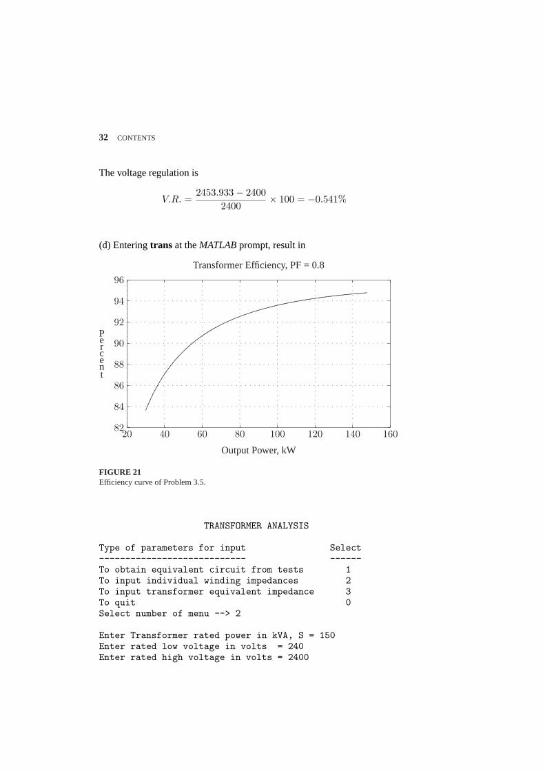
32 CONTENTS
Thevoltage regulation is
V.R. =2453.933− 2400
2400× 100 = −0.541%
(d) Enteringtrans at theMATLABprompt, result in
82
84
86
88
90
92
94
96
Percent
20 40 60 80 100 120 140 160
Output Power, kW
Transformer Efficiency, PF = 0.8
............................................................................................................................................................................................................................................................................................................
...................................
.......................................
...............................................
..........................................................
............................................................................
.............................................................................................................
...............................................................................................................................
.
.
.
.
.
.
.
.
.
.
.
.
.
.
.
.
.
.
.
.
.
.
.
.
.
.
.
.
.
.
.
.
.
.
.
.
.
.
.
.
.
.
.
.
.
.
.
.
.
.
.
.
.
.
.
.
.
.
.
.
.
.
.
.
.
.
.
.
.
.
.
.
.
.
.
.
.
.
.
.
.
.
.
.
.
.
.
.
.
.
.
.
.
.
.
.
.
.
.
.
.
.
.
.
.
.
.
.
.
.
.
.
.
.
.
.
.
.
.
.
.
.
.
.
.
.
.
.
.
.
.
.
.
.
.
.
.
.
.
.
.
.
.
.
.
.
.
.
.
.
.
.
.
.
.
.
.
.
.
.
.
.
.
.
.
.
.
.
.
.
.
.
.
.
.
.
.
.
.
.
.
.
.
.
.
.
.
.
.
.
.
.
.
.
.
.
.
.
.
.
.
.
.
.
.
.
.
.
.
.
.
.
.
.
.
.
.
.
.
.
.
.
.
.
.
.
.
.
.
.
.
. . . . . . . . . . . . . . . . . . . . . . . . . . . . . . . . . . . . . . . . . . . . . . . . . . . . . . . . . .
. . . . . . . . . . . . . . . . . . . . . . . . . . . . . . . . . . . . . . . . . . . . . . . . . . . . . . . . . .
. . . . . . . . . . . . . . . . . . . . . . . . . . . . . . . . . . . . . . . . . . . . . . . . . . . . . . . . . .
. . . . . . . . . . . . . . . . . . . . . . . . . . . . . . . . . . . . . . . . . . . . . . . . . . . . . . . . . .
. . . . . . . . . . . . . . . . . . . . . . . . . . . . . . . . . . . . . . . . . . . . . . . . . . . . . . . . . .
. . . . . . . . . . . . . . . . . . . . . . . . . . . . . . . . . . . . . . . . . . . . . . . . . . . . . . . . . .
FIGURE 21Efficiency curve of Problem 3.5.
TRANSFORMER ANALYSIS
Type of parameters for input Select---------------------------- ------To obtain equivalent circuit from tests 1To input individual winding impedances 2To input transformer equivalent impedance 3To quit 0Select number of menu --> 2
Enter Transformer rated power in kVA, S = 150Enter rated low voltage in volts = 240Enter rated high voltage in volts = 2400
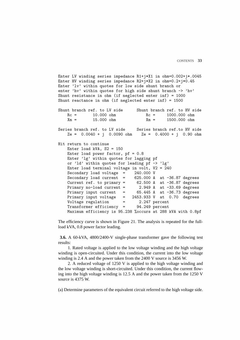
CONTENTS 33
Enter LV winding series impedance R1+j*X1 in ohm=0.002+j*.0045Enter HV winding series impedance R2+j*X2 in ohm=0.2+j*0.45Enter ’lv’ within quotes for low side shunt branch orenter ’hv’ within quotes for high side shunt branch -> ’hv’Shunt resistance in ohm (if neglected enter inf) = 1000Shunt reactance in ohm (if neglected enter inf) = 1500
Shunt branch ref. to LV side Shunt branch ref. to HV sideRc = 10.000 ohm Rc = 1000.000 ohmXm = 15.000 ohm Xm = 1500.000 ohm
Series branch ref. to LV side Series branch ref.to HV sideZe = 0.0040 + j 0.0090 ohm Ze = 0.4000 + j 0.90 ohm
Hit return to continueEnter load kVA, S2 = 150Enter load power factor, pf = 0.8Enter ’lg’ within quotes for lagging pfor ’ld’ within quotes for leading pf -> ’lg’Enter load terminal voltage in volt, V2 = 240Secondary load voltage = 240.000 VSecondary load current = 625.000 A at -36.87 degreesCurrent ref. to primary = 62.500 A at -36.87 degreesPrimary no-load current = 2.949 A at -33.69 degreesPrimary input current = 65.445 A at -36.73 degreesPrimary input voltage = 2453.933 V at 0.70 degreesVoltage regulation = 2.247 percentTransformer efficiency = 94.249 percentMaximum efficiency is 95.238 %occurs at 288 kVA with 0.8pf
The efficiency curve is shown in Figure 21. The analysis is repeated for the full-load kVA, 0.8 power factor leading.
3.6. A 60-kVA, 4800/2400-V single-phase transformer gave the following testresults:
1. Rated voltage is applied to the low voltage winding and the high voltagewinding is open-circuited. Under this condition, the current into the low voltagewinding is 2.4 A and the power taken from the 2400 V source is 3456 W.
2. A reduced voltage of 1250 V is applied to the high voltage winding andthe low voltage winding is short-circuited. Under this condition, the current flow-ing into the high voltage winding is 12.5 A and the power taken from the 1250 Vsource is 4375 W.
(a) Determine parameters of the equivalent circuit referred to the high voltage side.

34 CONTENTS
(b) Determine voltage regulation and efficiency when transformer is operating atfull-load, 0.8 power factor lagging, and a terminal voltage of 2400 V.
(c) What is the load kVA for maximum efficiency and the maximum efficiency at0.8 power factor?
(d) Determine the efficiency when transformer is operating at 3/4 full-load, 0.8power factor lagging, and a terminal voltage of 2400 V.
(e) Verify your answers by running thetrans program inMATLABand obtain thetransformer efficiency curve.
(a) From the no-load test data
RcLV =|V2|2P0
=(2400)2
3456= 1666.667 Ω
Ic =|V2|
RcLV=
24001666.67
= 1.44 A
Im =√
I20 − I2
c =√
(2.4)2 − (1.44)2 = 1.92 A
XmLV =|V2|Im
=24001.92
= 1250 Ω
The shunt parameters referred to the high-voltage side are
RCHV =(
48002400
)2
1666.667 = 6666.667 Ω
XmHV =(
48002400
)2
1250 = 5000 Ω
From the short-circuit test data
Ze1 =Vsc
Isc=
125012.5
= 100 Ω
Re1 =Psc
(Isc)2=
4375(12.5)2
= 28 Ω

CONTENTS 35
Xe1 =√
Z2e1 −R2
e1 =√
(100)2 − (28)2 = 96 Ω
(b) At full-load 0.8 power factor laggingS = 606 36.87 kVA, and the referredprimary current is
I2′=
S∗
V ∗ =600006 −36.87
4800= 12.56 −36.87 A
V1 = 4800 + (28 + j96)(12.56 −36.87) = 5848.296 7.368 V
Thevoltage regulation is
V.R. =5848.29− 4800
4800× 100 = 21.839%
Efficiency at full-load, 0.8 power factor is
η =(60)(0.8)
(60)(0.8) + 3.456 + 4.375× 100 = 85.974 %
(c) At Maximum efficiencyPc = Pcu, and we have
Pcu ∝ S2fl
Pc ∝ S2maxη
Therefore, the load kVA at maximum efficiency is
Smaxη =
√Pc
PcuSfl =
√34564375
60 = 53.327 kVA
and the maximum efficiency at 0.8 power factor is
η =(53.327)(0.8)
(53.327)(0.8) + 3.456 + 3.456× 100 = 86.057 %
(d) At 3/4 full-load, the copper loss is
Pcu3/4 = (3/4)2(4375) = 2460.9375 W
Therefore, the efficiency at3/4 full-load, 0.8 power factor is
η =(45)(0.8)
(45)(0.8) + 3.456 + 2.4609× 100 = 85.884 %
(e) The commandstrans display the following menu

36 CONTENTS
TRANSFORMER ANALYSIS
Type of parameters for input Select---------------------------- ------To obtain equivalent circuit from tests 1To input individual winding impedances 2To input transformer equivalent impedance 3To quit 0Select number of menu --> 1
Enter Transformer rated power in kVA, S = 60Enter rated low voltage in volts = 2400Enter rated high voltage in volts = 4800
Open circuit test data----------------------Enter ’lv’ within quotes for data referred to low side orenter ’hv’ within quotes for data referred to high side ->’lv’Enter input voltage in volts, Vo = 2400Enter no-load current in Amp, Io = 2.4Enter no-load input power in Watt, Po = 3456
Short circuit test data------------------------Enter ’lv’ within quotes for data referred to low side orenter ’hv’ within quotes for data referred to high side ->’hv’Enter reduced input voltage in volts, Vsc = 1250Enter input current in Amp, Isc = 12.5Enter input power in Watt, Psc = 4375
Shunt branch ref. to LV side Shunt branch ref. to HV sideRc = 1666.667 ohm Rc = 6666.667 ohmXm = 1250.000 ohm Xm = 5000.000 ohm
Series branch ref. to LV side Series branch ref.to HV sideZe = 7.0000 + j 24.0000 ohm Ze = 28.000 + j 96.000 ohm
Hit return to continueEnter load KVA, S2 = 60Enter load power factor, pf = 0.8Enter ’lg’ within quotes for lagging pfor ’ld’ within quotes for leading pf -> ’lg’Enter load terminal voltage in volt, V2 = 2400Secondary load voltage = 2400.000 VSecondary load current = 25.000 A at -36.87 degrees
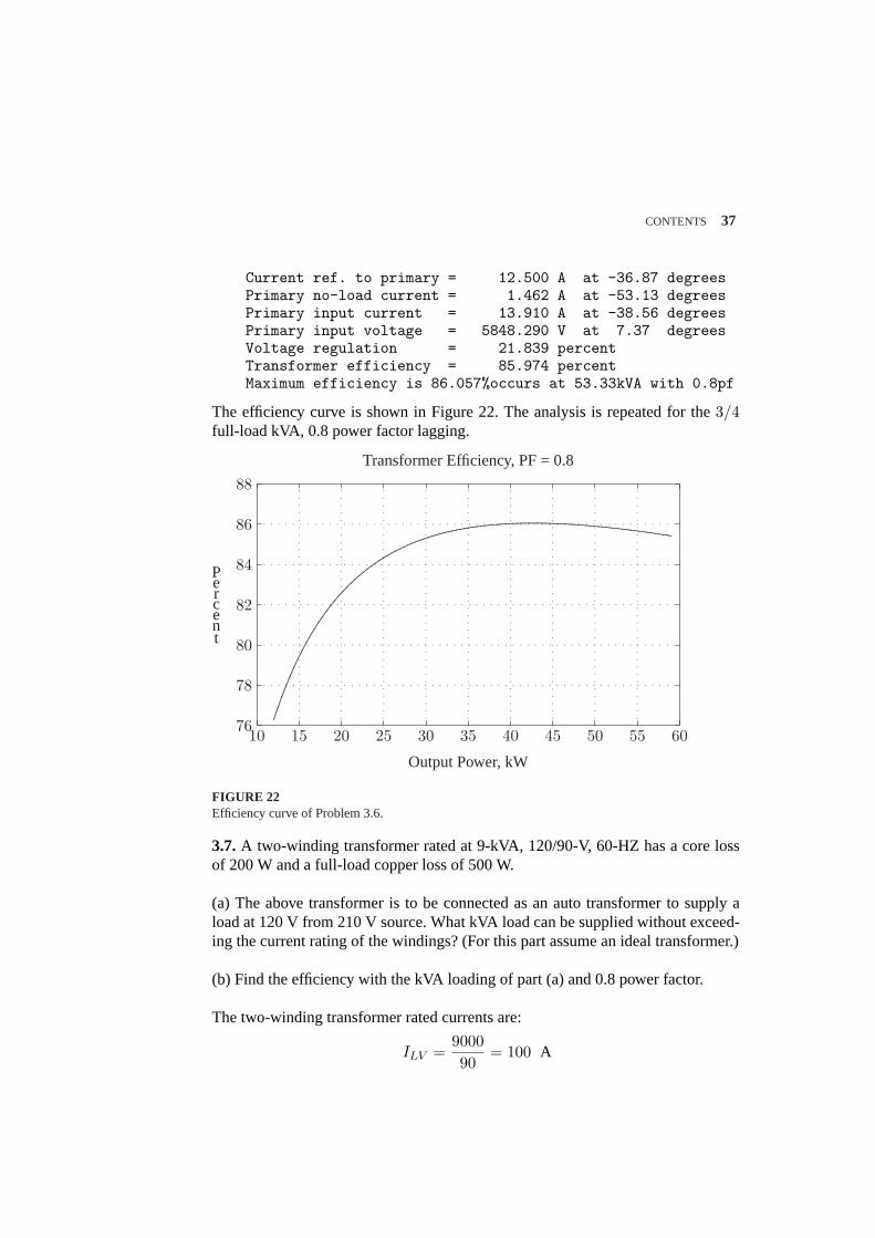
CONTENTS 37
Current ref. to primary = 12.500 A at -36.87 degreesPrimary no-load current = 1.462 A at -53.13 degreesPrimary input current = 13.910 A at -38.56 degreesPrimary input voltage = 5848.290 V at 7.37 degreesVoltage regulation = 21.839 percentTransformer efficiency = 85.974 percentMaximum efficiency is 86.057%occurs at 53.33kVA with 0.8pf
The efficiency curve is shown in Figure 22. The analysis is repeated for the3/4full-load kVA, 0.8 power factor lagging.
76
78
80
82
84
86
88
Percent
10 15 20 25 30 35 40 45 50 55 60
Output Power, kW
Transformer Efficiency, PF = 0.8
...............................................................................................................................................................................................................................................................................................................................................................................
..................................
...............................................
...........................................................................
....................................................................................................................................................................................................................................................................................................................................................................
.
.
.
.
.
.
.
.
.
.
.
.
.
.
.
.
.
.
.
.
.
.
.
.
.
.
.
.
.
.
.
.
.
.
.
.
.
.
.
.
.
.
.
.
.
.
.
.
.
.
.
.
.
.
.
.
.
.
.
.
.
.
.
.
.
.
.
.
.
.
.
.
.
.
.
.
.
.
.
.
.
.
.
.
.
.
.
.
.
.
.
.
.
.
.
.
.
.
.
.
.
.
.
.
.
.
.
.
.
.
.
.
.
.
.
.
.
.
.
.
.
.
.
.
.
.
.
.
.
.
.
.
.
.
.
.
.
.
.
.
.
.
.
.
.
.
.
.
.
.
.
.
.
.
.
.
.
.
.
.
.
.
.
.
.
.
.
.
.
.
.
.
.
.
.
.
.
.
.
.
.
.
.
.
.
.
.
.
.
.
.
.
.
.
.
.
.
.
.
.
.
.
.
.
.
.
.
.
.
.
.
.
.
.
.
.
.
.
.
.
.
.
.
.
.
.
.
.
.
.
.
.
.
.
.
.
.
.
.
.
.
.
.
.
.
.
.
.
.
.
.
.
.
.
.
.
.
.
.
.
.
.
.
.
.
.
.
.
.
.
.
.
.
.
.
.
.
.
.
.
.
.
.
.
.
.
.
.
.
.
.
.
.
.
.
.
.
. . . . . . . . . . . . . . . . . . . . . . . . . . . . . . . . . . . . . . . . . . . . . . . . . . . . . . . . . .
. . . . . . . . . . . . . . . . . . . . . . . . . . . . . . . . . . . . . . . . . . . . . . . . . . . . . . . . . .
. . . . . . . . . . . . . . . . . . . . . . . . . . . . . . . . . . . . . . . . . . . . . . . . . . . . . . . . . .
. . . . . . . . . . . . . . . . . . . . . . . . . . . . . . . . . . . . . . . . . . . . . . . . . . . . . . . . . .
. . . . . . . . . . . . . . . . . . . . . . . . . . . . . . . . . . . . . . . . . . . . . . . . . . . . . . . . . .
FIGURE 22Efficiency curve of Problem 3.6.
3.7.A two-winding transformer rated at 9-kVA, 120/90-V, 60-HZ has a core lossof 200 W and a full-load copper loss of 500 W.
(a) The above transformer is to be connected as an auto transformer to supply aload at 120 V from 210 V source. What kVA load can be supplied without exceed-ing the current rating of the windings? (For this part assume an ideal transformer.)
(b) Find the efficiency with the kVA loading of part (a) and 0.8 power factor.
The two-winding transformer rated currents are:
ILV =900090
= 100 A
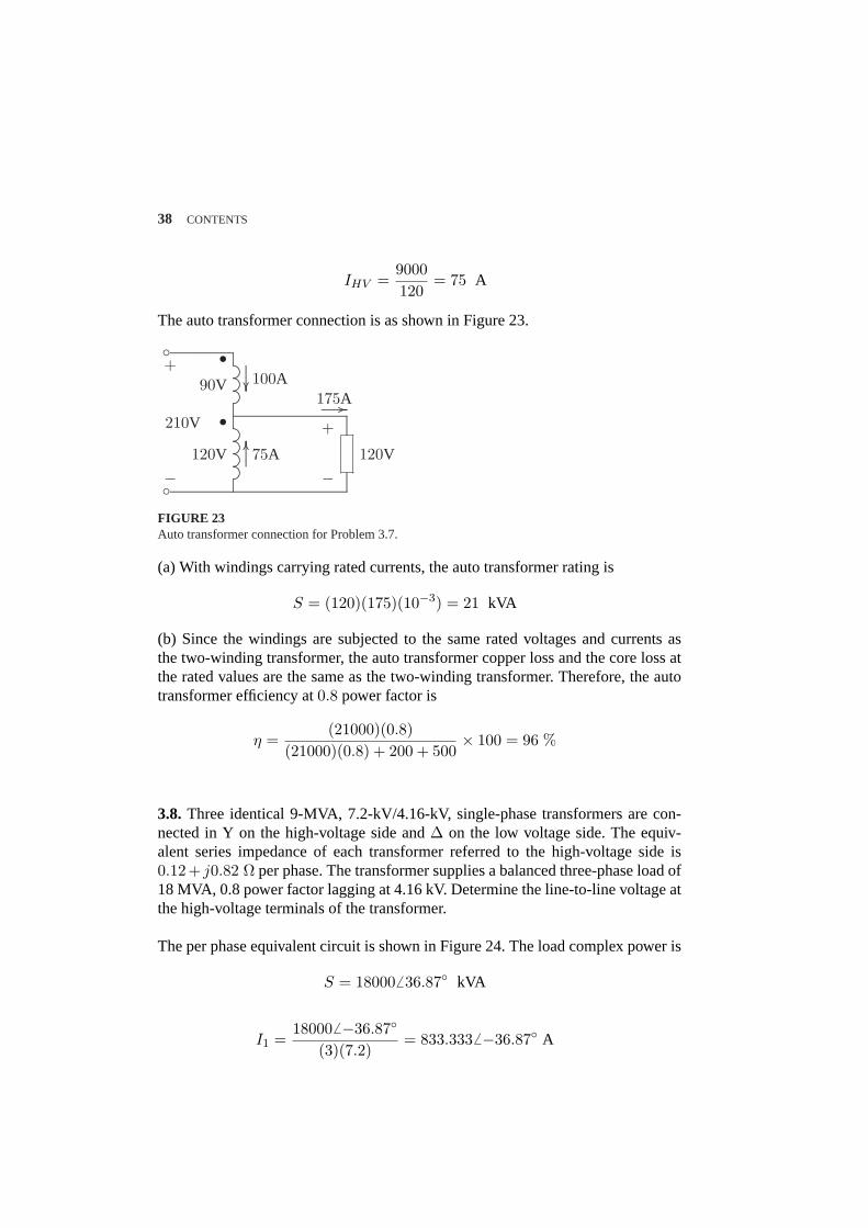
38 CONTENTS
IHV =9000120
= 75 A
The auto transformer connection is as shown in Figure 23.
...................................................................................................................................
.................................................................................................................................................................................................................................................................................................................................................
............................................
.....................................................................................................................................................................................................................................
.........................................................................................................
............................................................................................................................................
........
........
......
....................................................
........
........
........
........
........
........
........
........
....................
................
............................................................ ................
210V
90V
120V
100A
75A
175A
+
−
+
−120V
•
•
FIGURE 23Auto transformer connection for Problem 3.7.
(a) With windings carrying rated currents, the auto transformer rating is
S = (120)(175)(10−3) = 21 kVA
(b) Since the windings are subjected to the same rated voltages and currents asthe two-winding transformer, the auto transformer copper loss and the core loss atthe rated values are the same as the two-winding transformer. Therefore, the autotransformer efficiency at0.8 power factor is
η =(21000)(0.8)
(21000)(0.8) + 200 + 500× 100 = 96 %
3.8. Three identical 9-MVA, 7.2-kV/4.16-kV, single-phase transformers are con-nected in Y on the high-voltage side and∆ on the low voltage side. The equiv-alent series impedance of each transformer referred to the high-voltage side is0.12+ j0.82 Ω per phase. The transformer supplies a balanced three-phase load of18 MVA, 0.8 power factor lagging at 4.16 kV. Determine the line-to-line voltage atthe high-voltage terminals of the transformer.
The per phase equivalent circuit is shown in Figure 24. The load complex power is
S = 180006 36.87 kVA
I1 =180006 −36.87
(3)(7.2)= 833.3336 −36.87 A

CONTENTS 39
......................................................................................................................................
.......................................................................
................. ......................... ...........
.............. ......................... ...........
..............
....................................................................................................................................................................................................................................................................................................................................
............................................................................................................................
Ze1 = 0.12 + j0.82
V1 V ′2 = 7200 V
I1
........................................ ................
+
−
b
bFIGURE 24The per phase equivalent circuit of Problem 3.8.
V1 = 7.2 6 0 + (0.12 + j0.82)(833.3336 −36.87)(10−3)= 7.70546 3.62 kV
Therefore,the magnitude of the primary line-to-line supply voltage isV1LL =√3(7.7054) = 13.346 kV.
3.9.A 400-MVA, 240-kV/24-KV, three-phase Y-∆ transformer has an equivalentseries impedance of1.2 + j6 Ω per phase referred to the high-voltage side. Thetransformer is supplying a three-phase load of 400-MVA, 0.8 power factor laggingat a terminal voltage of 24 kV (line to line) on its low-voltage side. The primaryis supplied from a feeder with an impedance of0.6 + j1.2 Ω per phase. Deter-mine the line-to-line voltage at the high-voltage terminals of the transformer andthe sending-end of the feeder.
The per phase equivalent circuit referred to the primary is is shown in Figure 25.The load complex power is
......................................................................................................................................
.......................................................................
................. ......................... ...........
.............. ......................... ...........
.............. ............................................................................. ......................................................................
.....................................................................................................................................................................................................................................................................................
........................................................................................................................................................................................................................................................................................................................................................................................................................
+
−
V1
........................................................................
.......................................................................
................. ......................... ...........
.............. ......................... ...........
.............. .........................................................................................................................................................................................................
Zf = 0.6 + j1.2 Ze1 = 1.2 + j6
Vs V ′2 = 138.564 kV
I1
........................................ ................
+
−
b
bFIGURE 25The per phase equivalent circuit for Problem 3.9.
S = 4000006 36.87 kVA
40 CONTENTS
andthe referred secondary voltage per phase is
V′2 =
240√3
= 138.564 kV
I1 =4000006 −36.87
(3)(138.564)= 962.256 −36.87 A
V1 = 138.5646 0 + (1.2 + j6)(962.256 −36.87)(10−3) = 1436 1.57 kV
Therefore,the line-to-line voltage magnitude at the high voltage terminal of thetransformer isV1LL =
√3(143) = 247.69 kV.
Vs = 138.5646 0 + (1.8 + j7.2)(962.256 −36.87)(10−3) = 144.1776 1.79 kV
Therefore,the line-to-line voltage magnitude at the sending end of the feeder isV1LL =
√3(143) = 249.72 kV.
3.10.In Problem 3.9, with transformer rated values as base quantities, express allimpedances in per unit. Working with per-unit values, determine the line-to-linevoltage at the high-voltage terminals of the transformer and the sending-end of thefeeder.
With the transformer rated MVA as base, the HV-side base impedance is
ZB =(240)2
400= 144 Ω
The transformer and the feeder impedances in per unit are
Ze =(1.2 + j6)
144= 0.008333 + j0.04166 pu
Zf =(0.6 + j1.2)
144= 0.004166 + j0.00833 pu
I =1 6 −36.87
16 0= 16 −36.87 pu
V1 = 1.06 0 + (0.008333 + j0.04166)(16 −36.87 = 1.032056 1.57 pu

CONTENTS 41
Therefore,the line-to-line voltage magnitude at the high-voltage terminal of thetransformer is(1.03205)(240) = 247.69 kV
Vs = 1.06 0 + (0.0125 + j0.05)(16 −36.87 = 1.04056 1.79 pu
Therefore,the line-to-line voltage magnitude at the high voltage terminal of thetransformer is(1.0405)(240) = 249.72 kV
3.11.A three-phase, Y-connected, 75-MVA, 27-kV synchronous generator has asynchronous reactance of9.0 Ω per phase. Using rated MVA and voltage as basevalues, determine the per unit reactance. Then refer this per unit value to a 100-MVA, 30-kV base.
The base impedance is
ZB =(KVB)2
MV AB=
(27)2
75= 9.72 Ω
Xpu =9
9.72= 0.926 pu
The generator reactance on a 100-MVA, 30-kV base is
Xpunew = 0.926(
10075
) (2730
)2
= 1.0 pu
3.12.A 40-MVA, 20-kV/400-kV, single-phase transformer has the following seriesimpedances:
Z1 = 0.9 + j1.8 Ω and Z2 = 128 + j288 ΩUsing the transformer rating as base, determine the per unit impedance of the trans-former from the ohmic value referred to the low-voltage side. Compute the per unitimpedance using the ohmic value referred to the high-voltage side.
The transformer equivalent impedance referred to the low-voltage side is
Ze1 = 0.9 + j1.8 +(
20400
)2
(128 + j288) = 1.22 + j2.52 Ω
The low-voltage base impedance is
ZB1 =(20)2
40= 10 Ω
Zpu1 =1.22 + j2.52
10= 0.122 + j0.252 pu

42 CONTENTS
Thetransformer equivalent impedance referred to the high-voltage side is
Ze2 =(
40020
)2
(0.9 + j1.8) + (128 + j288) = 488 + j1008 Ω
The high-voltage base impedance is
ZB2 =(400)2
40= 4000 Ω
Zpu2 =488 + j1008
4000= 0.122 + j0.252 pu
We note that the transformer per unit impedance has the same value regardless ofwhether it is referred to the primary or the secondary side.
3.13.Draw an impedance diagram for the electric power system shown in Figure26 showing all impedances in per unit on a 100-MVA base. Choose 20 kV as thevoltage base for generator. The three-phase power and line-line ratings are givenbelow.
G1 : 90 MVA 20 kV X = 9%T1 : 80 MVA 20/200 kV X = 16%T2 : 80 MVA 200/20 kV X = 20%G2 : 90 MVA 18 kV X = 9%Line: 200 kV X = 120 ΩLoad: 200 kV S = 48 MW +j64 Mvar
.............................................
.......
.............................................
.......
........................................................................................................
.............................................
.......
.............................................
.......
........................................................................................................
?½¼
¾»
½¼
¾»G1
T1 T2
G2
1 2Line
Load
FIGURE 26One-line diagram for Problem 3.13
The base voltageVBG1on the LV side ofT1 is 20 kV. Hence the base on its HVside is
VB1 = 20(
20020
)= 200 kV
This fixes the base on the HV side ofT2 atVB2 = 200 kV, and on its LV side at
VBG2 = 200(
20200
)= 20 kV

CONTENTS 43
The generator and transformer reactances in per unit on a 100 MVA base,from (3.69)and (3.70) are
G: X = 0.09(
10090
)= 0.10 pu
T1: X = 0.16(
10080
)= 0.20 pu
T2: X = 0.20(
10080
)= 0.25 pu
G2: X = 0.09(
10090
) (1820
)2
= 0.081 pu
The base impedance for the transmission line is
ZBL =(200)2
100= 400 Ω
The per unit line reactance is
Line: X =(
120400
)= 0.30 pu
The load impedance in ohms is
ZL =(VL−L)2
S∗L(3φ)
=(200)2
48− j64= 300 + j400 Ω
The load impedance in per unit is
ZL(pu) =300 + j400
400= 0.75 + j1.0 pu
The per unit equivalent circuit is shown in Figure 27.
µ´¶³G1
j0.1.......................
.........................
.........................
..
µ´¶³G2
j0.081.......................
.........................
.........................
..
....................................
.......................................
j0.2....................................
.......................................
j0.3....................................
.......................................
j0.25
0.75 + j1.0
FIGURE 27Per unit impedance diagram for Problem 3.11.

44 CONTENTS
.............................................
............
.............................................
............
..................................................................................................................
.............................................
............
.............................................
............
..................................................................................................................
.............................................
............
.............................................
............
..................................................................................................................
.............................................
............
.............................................
............
.............................................
............
.............................................
............
................................................................................................................................................................................................................
?
½¼
¾»
½¼
¾»G
T1 T2
T3
T4 M
1 2 3 4
5 6
Line 1
Line 2
Load
220 kV
110 kV
FIGURE 28One-line diagram for Problem 3.14
3.14.The one-line diagram of a power system is shown in Figure 28.The three-phase power and line-line ratings are given below.
G: 80 MVA 22 kV X = 24%T1: 50 MVA 22/220 kV X = 10%T2: 40 MVA 220/22 kV X = 6.0%T3: 40 MVA 22/110 kV X = 6.4%Line 1: 220 kV X = 121 ΩLine 2: 110 kV X = 42.35 ΩM : 68.85 MVA 20 kV X = 22.5%Load: 10 Mvar 4 kV ∆-connected capacitors
The three-phase ratings of the three-phase transformer arePrimary: Y-connected 40MVA, 110 kVSecondary: Y-connected 40 MVA, 22 kVTertiary: ∆-connected 15 MVA, 4 kV
The per phase measured reactances at the terminal of a winding with the secondone short-circuited and the third open-circuited are
ZPS = 9.6% 40 MVA, 110 kV / 22 kVZPT = 7.2% 40 MVA, 110 kV / 4 kVZST = 12% 40 MVA, 22 kV / 4 kV
Obtain the T-circuit equivalent impedances of the three-winding transformer to thecommon MVA base. Draw an impedance diagram showing all impedances in perunit on a 100-MVA base. Choose 22 kV as the voltage base for generator.
The base voltageVB1 on the LV side ofT1 is 22 kV. Hence the base on its HV side
CONTENTS 45
is
VB2 = 22(
22022
)= 220 kV
This fixes the base on the HV side ofT2 atVB3 = 220 kV, and on its LV side at
VB4 = 220(
22220
)= 22 kV
Similarly, the voltage base at buses 5 and 6 are
VB5 = VB6 = 22(
11022
)= 110 kV
Voltage base for the tertiary side ofT4 is
VBT = 110(
4110
)= 4 kV
The per unit impedances on a 100 MVA base are:
G: X = 0.24(
10080
)= 0.30 pu
T1: X = 0.10(
10050
)= 0.20 pu
T2: X = 0.06(
10040
)= 0.15 pu
T3: X = 0.064(
10040
)= 0.16 pu
The motor reactance is expressed on its nameplate rating of 68.85 MVA, and 20kV. However, the base voltage at bus 4 for the motor is 22 kV, therefore
M : X = 0.225(
10068.85
) (2022
)2
= 0.27 pu
Impedance bases for lines 1 and 2 are
ZB2 =(220)2
100= 484 Ω
ZB5 =(110)2
100= 121 Ω

46 CONTENTS
............................. ..........
................... ............................. ..........
................... ............................. ..........
................... ............................. ..........
................... .............................
............................. ..........
................... ............................. ..........
................... ............................. ..........
................... ............................. ..........
................... ............................. ..........
................... ............................. ..........
................................................
.............................
.............................
µ´¶³ .............
..........................................................................
.............................
.............................
.............................
?Im
µ´¶³
G M
1 4j0.20 j0.25 j0.15
j0.16 j0.35 j0.06 j0.18j0.3 j0.27
0.12
−j10Eg Em
-I
FIGURE 29Per unit impedance diagram for Problem 3.14.
Line 1 and 2 per unit reactances are
Line1: X =(
121484
)= 0.25 pu
Line2: X =(
42.35121
)= 0.35 pu
The load impedance in ohms is
ZL =(VL−L)2
S∗L(3φ)
=(4)2
j10= −j1.6 Ω
The base impedance for the load is
ZBT =(4)2
100= 0.16 Ω
Therefore, the load impedance in per unit is
ZL(pu) =−j1.60.16
= −j10 pu
Thethree-winding impedances on a 100 MVA base are
ZPS = 0.096(
10040
)= 0.24 pu
ZPT = 0.072(
10040
)= 0.18 pu
ZST = 0.120(
10040
)= 0.30 pu

CONTENTS 47
Theequivalent T circuit impedances are
ZP =12(j0.24 + j0.18− j0.30) = j0.06 pu
ZS =12(j0.24 + j0.30− j0.18) = j0.18 pu
ZT =12(j0.18 + j0.30− j0.24) = j0.12 pu
The per unit equivalent circuit is shown in Figure 29.
3.15. The three-phase power and line-line ratings of the electric power systemshown in Figure 30 are given below.
.............................................
............
.............................................
............
..................................................................................................................
.........................................................
.............................................
............
..................................................................................................................½¼
¾»
½¼
¾»G
Vg VmT1 T2
M
1 2Line
FIGURE 30One-line diagram for Problem 3.15
G1 : 60 MVA 20 kV X = 9%T1 : 50 MVA 20/200 kV X = 10%T2 : 50 MVA 200/20 kV X = 10%M : 43.2 MVA 18 kV X = 8%Line: 200 kV Z = 120 + j200 Ω
(a) Draw an impedance diagram showing all impedances in per unit on a 100-MVAbase. Choose 20 kV as the voltage base for generator.
(b) The motor is drawing 45 MVA, 0.80 power factor lagging at a line-to-line ter-minal voltage of 18 kV. Determine the terminal voltage and the internal emf of thegenerator in per unit and in kV.
The base voltageVBG1on the LV side ofT1 is 20 kV. Hence the base on its HVside is
VB1 = 20(
20020
)= 200 kV
This fixes the base on the HV side ofT2 atVB2 = 200 kV, and on its LV side at
VBm = 200(
20200
)= 20 kV

48 CONTENTS
The generator and transformer reactances in per unit on a 100 MVA base,from (3.69)and (3.70) are
G: X = 0.09(
10060
)= 0.15 pu
T1: X = 0.10(
10050
)= 0.20 pu
T2: X = 0.10(
10050
)= 0.20 pu
M : X = 0.08(
10043.2
) (1820
)2
= 0.15 pu
The base impedance for the transmission line is
ZBL =(200)2
100= 400 Ω
The per unit line impedance is
Line: Zline = (120 + j200
400) = 0.30 + j0.5 pu
The per unit equivalent circuit is shown in Figure 31.
µ´¶³Eg
j0.15 Vg
+
−
Vm
+
−
.......................................................................................
µ´¶³Em
j0.15.......................................................................................
.......................................
................................................
j0.2...........................................
..........................................
............................................
...................................................
................................................
0.3 + j0.5.......................................
................................................
j0.20
FIGURE 31Per unit impedance diagram for Problem 3.15.
(b) The motor complex power in per unit is
Sm =456 36.87
100= 0.456 36.87 pu
andthe motor terminal voltage is
Vm =186 0
20= 0.906 0 pu

CONTENTS 49
I =0.456 −36.87
0.906 0= 0.56 −36.87 pu
Vg = 0.906 0 + (0.3 + j0.9)(0.56 −36.87 = 1.317956 11.82 pu
Thus,the generator line-to-line terminal voltage is
Vg = (1.31795)(20) = 26.359 kV
Eg = 0.906 0 + (0.3 + j1.05)(0.5 6 −36.87 = 1.3756 13.88 pu
Thus,the generator line-to-line internal emf is
Eg = (1.375)(20) = 27.5 kV
3.16.The one-line diagram of a three-phase power system is as shown in Figure 32.Impedances are marked in per unit on a 100-MVA, 400-kV base. The load at bus2is S2 = 15.93 MW −j33.4 Mvar, and at bus3 is S3 = 77 MW +j14 Mvar. It isrequired to hold the voltage at bus3 at4006 0 kV. Working in per unit, determinethe voltage at buses2 and1.
? ?
V1 V2 V3
S2 S3
j0.5 pu j0.4 pu
FIGURE 32One-line diagram for Problem 3.16
S2 = 15.93 MW − j33.4 Mvar = 0.1593− j0.334 pu
S3 = 77.00 MW + j14.0 Mvar = 0.7700 + j0.140 pu
V3 =4006 0
400= 1.06 0 pu
I3 =S∗3V ∗
3
=0.77− j0.14
1.06 0= 0.77− j0.14 pu
V2 = 1.0 6 0 + (j0.4)(0.77− j0.14) = 1.16 16.26 pu

50 CONTENTS
Therefore,the line-to-line voltage at bus 2 is
V2 = (400)(1.1) = 440 kV
I2 =S∗2V ∗
2
=0.1593 + j0.334
1.16 −16.26= 0.054 + j0.332 pu
I12 = (0.77− j0.14) + (0.054 + j0.332) = 0.824 + j0.192 pu
V1 = 1.16 16.26 + (j0.5)(0.824 + j0.192) = 1.26 36.87 pu
Therefore,the line-to-line voltage at bus 1 is
V1 = (400)(1.2) = 480 kV
3.17.The one-line diagram of a three-phase power system is as shown in Figure33. The transformer reactance is20 percent on a base of 100-MVA, 23/115-kV andthe line impedance isZ = j66.125Ω. The load at bus2 is S2 = 184.8 MW +j6.6Mar, and at bus3 is S3 = 0 MW +j20 Mar. It is required to hold the voltage at bus3 at1156 0 kV. Working in per unit, determine the voltage at buses2 and1.
..............................................................................................
..........
............................................................
............................................
??
V1
V2
V3
S2
S3
j66.125 Ω
FIGURE 33One-line diagram for Problem 3.17
S2 = 184.8 MW + j6.6 Mvar = 1.848 + j0.066 pu
S3 = 0 MW + j20.0 Mvar = 0 + j0.20 pu
V3 =1156 0
115= 1.06 0 pu
I3 =S∗3V ∗
3
=−j0.21.06 0
= −j0.2 pu
V2 = 1.06 0 + (j0.5)(−j0.2) = 1.1 6 0 pu

CONTENTS 51
Therefore,the line-to-line voltage at bus 2 is
V2 = (115)(1.1) = 126.5 kV
I2 =S∗2V ∗
2
=1.848− j0.066
1.16 0= 1.68− j0.06 pu
I12 = (1.68− j0.06) + (−j0.2) = 1.68− j0.26 pu
V1 = 1.1 6 0 + (j0.2)(1.68− j0.26) = 1.26 16.26 pu
Therefore,the line-to-line voltage at bus 1 is
V1 = (23)(1.2) = 27.6 kV
CHAPTER4 PROBLEMS
4.1. A solid cylindrical aluminum conductor 25 km long has an area of 336,400circular mils. Obtain the conductor resistance at (a)20C and (b)50C. The resis-tivity of aluminum at20C is2.8× 10−8 Ω-m.
(a)
d =√
336400 = 580 mil = (580)(10−3)(2.54) = 1.4732 cm
A =πd2
4= 1.704564 cm2
R1 = ρ`
A= 2.8× 10⁻⁸ 25× 103
1.704564× 10−4= 4.106 Ω
(b)
R2 = R1
(228 + 50228 + 20
)= 4.106
(278248
)= 4.6 Ω
4.2. A transmission-line cable consists of 12 identical strands of aluminum, each3 mm in diameter. The resistivity of aluminum strand at20C is 2.8× 10⁻⁸ Ω-m.Find the50C AC resistance per Km of the cable. Assume a skin-effect correctionfactor of 1.02 at 60 Hz.
52

CONTENTS 53
A = 12πd2
4= 12
(π)(32)4
= 84.823 mm2
R20 = ρ`
A=
2.8× 10−8 × 103
84.823× 10−6= 0.33 Ω
R50 = R20
(228 + 50228 + 20
)= 0.33
(278248
)= 0.37 Ω
RAC = (1.02)(0.37) = 0.3774 Ω
4.3. A three-phase transmission line is designed to deliver 190.5-MVA at 220-kV over a distance of 63 Km. The total transmission line loss is not to exceed2.5 percent of the rated line MVA. If the resistivity of the conductor material is2.84 × 10−8 Ω-m, determine the required conductor diameter and the conductorsize in circular mils.
The total transmission line loss is
PL =2.5100
(190.5) = 4.7625 MW
|I| = S√3VL
=(190.5)103
√3(220)
= 500 A
FromPL = 3R|I|2, the line resistance per phase is
R =4.7625× 10⁶
3(500)2= 6.35 Ω
The conductor cross sectional area is
A =(2.84× 10⁻⁸)(63× 103)
6.35= 2.81764× 10⁻⁴ m2
Therefore
d = 1.894 cm = 0.7456 in = 556000 cmil

54 CONTENTS
4.4.A single-phase transmission line 35 Km long consists of two solid round con-ductors, each having a diameter of 0.9 cm. The conductor spacing is 2.5 m. Calcu-late the equivalent diameter of a fictitious hollow, thin-walled conductor having thesame equivalent inductance as the original line. What is the value of the inductanceper conductor?
r′= e−
14 r = e−
14
(0.92
)= 0.35 cm
or d = 0.7 cm.
L = 0.2 ln2.5
0.35× 10−2= 1.314 mH/Km
The inductance per conductor is`L = (35)(1.314) = 46 mH.
4.5.Find the geometric mean radius of a conductor in terms of the radiusr of anindividual strand for(a) Three equal strands as shown in Figure 34(a)(b) Four equal strands as shown in Figure 34(b)
"!
#Ã
"!
#Ã"!
#Ã
"!
#Ã
"!
#Ã"!
#Ã
"!
#Ã
(a) (b)
.................................................................
..........................
.................................................... .................................................... ............. ............. ............. .............
.............
.............
...........................................................................
......................................................................
..........................
..........................
...
FIGURE 34Cross section of the stranded conductor for Problem 4.5.
(a)
GMR = 9
√(r′2r × 2r)3
=3√
e−14 r × 2r × 2r = 1.46r
(b)
GMR = 16√
(r′ × 2r × 2r ×√
2 2r)4
=4√
e−14 8√
2 r4 = 1.723r

CONTENTS 55
4.6.Onecircuit of a single-phase transmission line is composed of three solid 0.5-cm radius wires. The return circuit is composed of two solid 2.5-cm radius wires.The arrangement of conductors is as shown in Figure 35. Applying the concept oftheGMD andGMR, find the inductance of the complete line in millihenry perkilometer.
m m m m m¾ -¾ -¾ -¾ -5 m 5 m 10 m 5 m︸ ︷︷ ︸
ConductorX︸ ︷︷ ︸ConductorY
FIGURE 35Conductor layout for Problem 4.6.
Dm = 6
√(20)(25)(15)(20)(10)(15) = 16.802 m
DSX = 9√
(e−14 × 0.005× 5× 10)(e−
14 × 0.005× 5× 5)(e−
14 × 0.005× 5× 10)
= 0.5366 m
DSY = 4
√(e−
14 × 0.025× 5
)2= 0.312 m
Therefore
LX = 0.2 ln16.8020.5366
= 0.6888 mH/Km
and
LY = 0.2 ln16.8020.312
= 0.79725 mH/Km
The loop inductance is
L = LX + LY = 0.6888 + 0.79725 = 1.48605 mH/Km
4.7. A three-phase, 60-Hz transposed transmission line has a flat horizontal con-figuration as shown in Figure 36. The line reactance is 0.486Ω per kilometer. Theconductor geometric mean radius is 2.0 cm. Determine the phase spacingD inmeter.

56 CONTENTS
m m m¾ -¾ -
¾ -
D D
2D
a b c
FIGURE 36Conductor layout for Problem 4.7.
L =(0.486)103
(2π)(60)= 1.2892 mH/Km
Therefore, we have
1.2892 = 0.2 lnGMD
0.02or GMD = 12.6 m
12.6 = 3
√(D)(D)(2D) or D = 10 m
4.8.A three-phase transposed line is composed of one ACSR 159,000 cmil, 54/19Lapwing conductor per phase with flat horizontal spacing of 8 meters as shown inFigure 37. TheGMR of each conductor is 1.515 cm.(a) Determine the inductance per phase per kilometer of the line.(b) This line is to be replaced by a two-conductor bundle with 8-m spacing mea-sured from the center of the bundles as shown in Figure 38. The spacing betweenthe conductors in the bundle is 40 cm. If the line inductance per phase is to be77 percent of the inductance in part (a), what would be theGMR of each newconductor in the bundle?
m m m¾ -¾ -
¾ -
D12 = 8 m D23 = 8 m
D13 = 16 m
a b c
FIGURE 37Conductor layout for Problem 4.8 (a).
(a)
GMD = 3
√(8)(8)(16) = 10.0794 m
L = 0.210.0794
1.515× 10−2= 1.3 mH/Km

CONTENTS 57
f f f f f f
¾ -¾ -
¾ -
- ¾40D12 = 8 m D23 = 8 m
D13 = 16 m
a b c.............
.............
.............
.....
.............
.............
.....
.............
.............
.............
.............
.........
FIGURE 38Conductor layout for Problem 4.8 (b).
(b)
L2 = (1.3)(0.77) = 1.0 mH/Km
1.0 = 0.2 ln10.0794
DbS
or DbS = 0.0679 m
Now
SbS =
√DS d therefore DS = 1.15 cm
4.9.A three-phase transposed line is composed of one ACSR 1,431,000 cmil, 47/7Bobolink conductor per phase with flat horizontal spacing of 11 meters as shownin Figure 39. The conductors have a diameter of 3.625 cm and aGMR of 1.439cm. The line is to be replaced by a three-conductor bundle of ACSR 477,000 cmil,26/7 Hawk conductors having the same cross-sectional area of aluminum as thesingle-conductor line. The conductors have a diameter of 2.1793 cm and aGMRof 0.8839 cm. The new line will also have a flat horizontal configuration, but it is tobe operated at a higher voltage and therefore the phase spacing is increased to 14m as measured from the center of the bundles as shown in Figure 40. The spacingbetween the conductors in the bundle is 45 cm. Determine(a) The percentage change in the inductance.(b) The percentage change in the capacitance.
m m m¾ -¾ -
¾ -
D12 = 11 m D23 = 11 m
D13 = 22 m
a b c
FIGURE 39Conductor layout for Problem 4.9 (a).

58 CONTENTS
f ff
f ff
f ff
¾ -¾ -
¾ -
- ¾45D12 = 14 m D23 = 14 m
D13 = 28 m
a b c
.............
.............
.............
.....
.............
.............
.....
.............
.............
.............
.............
.........
FIGURE 40Conductor layout for Problem 4.9 (b).
For the one conductor per phase configuration , we have
GMD = 3
√(11)(11)(22) = 13.859 m
L = 0.213.859
1.439× 10−2= 1.374 mH/Km
C =0.0556
ln 13.8591.8125×10−2
= 0.008374 µF/Km
For the three-conductor bundle per phase configuration , we have
GMD = 3
√(14)(14)(28) = 17.6389 m
GMRL = 3
√(45)2(0.8839) = 12.1416 cm
GMRC = 3
√(45)2(2.1793/2) = 13.01879 cm
L = 0.217.6389
12.1416× 10−2= 0.9957 mH/Km
C =0.0556
ln 17.638913.01879×10−2
= 0.011326 µF/Km
(a) The percentage reduction in the inductance is
1.374− 0.99571.374
(100) = 27.53%

CONTENTS 59
(b) The percentage increase in the capacitance is
0.001326− 0.0083740.008374
(100) = 35.25%
4.10.A single-circuit three-phase transmission transposed line is composed of fourACSR 1,272,000 cmil conductor per phase with horizontal configuration as shownin Figure 41. The bundle spacing is 45 cm. The conductor code name ispheasant.In MATLAB, use commandacsr to find the conductor diameter and itsGMR.Determine the inductance and capacitance per phase per kilometer of the line. Usefunction [GMD, GMRL, GMRC] =gmd , (4.58) and (4.92) inMATLABto verifyyour results.
h hh h
h hh h
h hh h
¾ -¾ -
¾ -
- ¾45D12 = 14 m D23 = 14 m
D13 = 28 m
a b c
.............
.............
.............
.............
.............
.............
.............
.............
.............
.............
.............
.............
......
FIGURE 41Conductor layout for Problem 4.10.
Using the commandacsr, result in
Enter ACSR code name within single quotes -> ’pheasant’Al Area Strand Diameter GMR Resistance Ohm/Km AmpacityCMILS Al/St cm cm 60Hz,25C 60HZ,50C Ampere1272000 54/19 3.5103 1.4173 0.04586 0.05290 1200
From (4.79)
GMD = 3
√(14)(14)(28) = 17.63889 m
and From (4.53) and (4.90), we have
GMRL = 1.09 4
√(1.4173)(45)3 = 20.66 cm
GMRC = 1.09 4
√(3.5103/2)(45)3 = 21.8 cm
and from (4.58) and (4.92), we get
L = 0.2 lnGMD
GMRL= 0.2 ln
17.638890.2066
= 0.889 mH/Km
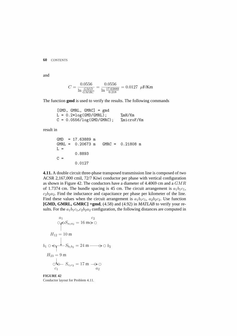
60 CONTENTS
and
C =0.0556
ln GMDGMRC
=0.0556
ln 17.638890.218
= 0.0127 µF/Km
The functiongmd is used to verify the results. The following commands
[GMD, GMRL, GMRC] = gmdL = 0.2*log(GMD/GMRL); %mH/KmC = 0.0556/log(GMD/GMRC); %microF/Km
result in
GMD = 17.63889 mGMRL = 0.20673 m GMRC = 0.21808 mL =
0.8893C =
0.0127
4.11.A double circuit three-phase transposed transmission line is composed of twoACSR 2,167,000 cmil, 72/7 Kiwi conductor per phase with vertical configurationas shown in Figure 42. The conductors have a diameter of 4.4069 cm and aGMRof 1.7374 cm. The bundle spacing is 45 cm. The circuit arrangement isa1b1c1,c2b2a2. Find the inductance and capacitance per phase per kilometer of the line.Find these values when the circuit arrangement isa1b1c1, a2b2c2. Use function[GMD, GMRL, GMRC] =gmd , (4.58) and (4.92) inMATLABto verify your re-sults. For thea1b1c1,c2b2a2 configuration, the following distances are computed in
ee ee
e e ee
e e eea1
b1
c1
c2
b2
a2
¾ -
¾ -
¾ -6
?6
?
Sa1a2 = 16 m
Sb1b2 = 24 m
Sc1c2 = 17 m
H12 = 10 m
H23 = 9 m
FIGURE 42Conductor layout for Problem 4.11.

CONTENTS 61
meter.
Da1b1 = 10.7703 Da1b2 = 22.3607 Da2b1 = 22.3886 Da2b2 = 9.6566Db1c1 = 9.6566 Db1c2 = 22.3607 Db2c1 = 22.3886 Db2c2 = 10.7703Da1c1 = 19.0065 Da1c2 = 16.0000 Da2c1 = 17.0000 Da2c2 = 19.0065Da1a2 = 25.1644 Db1b2 = 24.0000 Dc1c2 = 25.1644
From (4.54), we have
DAB = 4
√(10.7703)(22.3607)(22.3886)(9.6566) = 15.1057
DBC = 4
√(9.6566)(22.3607)(22.3886)(10.7703) = 15.1057
DCA = 4
√(19.0065)(16.0000)(17.0000)(19.0065) = 17.0749
The equivalent geometric mean distance is
GMD = 3
√(15.1057)(15.1057)(17.7049) = 15.9267
From (4.51) and (4.66), we have
Dbs =
√Ds × d =
√(0.017374)(0.45) = 0.08842
rb =√
r × d =√
(0.044069/2)(0.45) = 0.09957
From (4.56) and (4.93), we have
DSA =√
(0.08842)(25.1644) = 1.4916 DSB =√
(0.08842)(24.0000) = 1.4567DSC =
√(0.08842)(25.1644) = 1.4916
and
rA =√
(0.09957)(25.1644) = 1.5829 rB =√
(0.09957)(24.0000) = 1.5458rC =
√(0.09957)(25.1644) = 1.5829
GMRL = 3
√(1.4916)(1.4567)(1.4916) = 1.4799
GMRC = 3
√(1.5829)(1.5458)(1.5829) = 1.5705
Therefore, the inductance and capacitance per phase are
L = 0.2 lnGMD
GMRL= 0.2 ln
15.92671.4799
= 0.4752 mH/Km
and
C =0.0556
ln GMDGMRC
=0.0556
ln 15.92671.5705
= 0.0240 µF/Km
The functiongmd is used to verify the results. The following commands

62 CONTENTS
[GMD, GMRL, GMRC] = gmdL = 0.2*log(GMD/GMRL); %mH/KmC = 0.0556/log(GMD/GMRC); %microF/Km
result in
Circuit Arrangements--------------------(1) abc-c‘b‘a‘(2) abc-(a‘)(b‘)(c‘)Enter (1 or 2) -> 1Enter spacing unit within quotes ’m’ or ’ft’-> ’m’Enter row vector [S11, S22, S33] = [16 24 17]Enter row vector [H12, H23] = [10 9]Cond. size, bundle spacing unit: Enter ’cm’ or ’in’-> ’cm’Conductor diameter in cm = 4.4069Geometric Mean Radius in cm = 1.7374No. of bundled cond. (enter 1 for single cond.) = 2Bundle spacing in cm = 45
GMD = 15.92670 mGMRL = 1.47993 m GMRC = 1.57052 mL =
0.4752C =
0.0240
For thea1b1c1,a2b2c2 configuration, the following distances are computed in me-ter.
Da1b1 = 10.7703 Da1b2 = 22.3607 Da2b1 = 22.3607 Da2b2 = 10.7703Db1c1 = 9.6566 Db1c2 = 22.3886 Db2c1 = 22.3886 Db2c2 = 9.6566Da1c1 = 19.0065 Da1c2 = 25.1644 Da2c1 = 25.1644 Da2c2 = 19.0065Da1a2 = 16.0000 Db1b2 = 24.0000 Dc1c2 = 17.0000
From (4.54), we have
DAB = 4
√(10.7703)(22.3607)(22.3607)(10.7703) = 15.5187
DBC = 4
√(9.6566)(22.3886)(22.3886)(9.6566) = 14.7036
DCA = 4
√(19.0065)(25.1644)(25.1644)(19.0065) = 21.8698
The equivalent geometric mean distance is
GMD = 3
√(15.5187)(14.7036)(21.8698) = 17.0887

CONTENTS 63
From(4.51) and (4.66), we have
Dbs =
√Ds × d =
√(0.017374)(0.45) = 0.08842
rb =√
r × d =√
(0.044069/2)(0.45) = 0.09957
From (4.56) and (4.93), we have
DSA =√
(0.08842)(16) = 1.1894 DSB =√
(0.08842)(24.0000) = 1.4567DSC =
√(0.08842)(17) = 1.2260
and
rA =√
(0.09957)(16) = 1.2622 rB =√
(0.09957)(24.0000) = 1.5458rC =
√(0.09957)(17) = 1.3010
GMRL = 3
√(1.1894)(1.4567)(1.2260) = 1.2855
GMRC = 3
√(1.2622)(1.5458)(1.3010 = 1.3641
Therefore, the inductance and capacitance per phase are
L = 0.2 lnGMD
GMRL= 0.2 ln
17.08871.2855
= 0.5174 mH/Km
and
C =0.0556
ln GMDGMRC
=0.0556
ln 17.08871.3641
= 0.02199 µF/Km
The functiongmd is used in the same way as before to verify the results.
4.12.The conductors of a double-circuit three-phase transmission line are placedon the corner of a hexagon as shown in Figure 43. The two circuits are in paral-lel and are sharing the balanced load equally. The conductors of the circuits areidentical, each having a radiusr. Assume that the line is symmetrically transposed.Using the method ofGMR, determine an expression for the capacitance per phaseper meter of the line.
Da1c1 = Da1b2 = Db1a2 = Db1c2 = Dc1b2 = Dc2a2 =√
3D
DAB = DBC = DCA = 4
√Da1b1Da1b2Da2b1Da2b2
=√
Da1b1Da1b2 = 314 D

64 CONTENTS
k k
k k
k k¾ -
¾ -
¾ -
D
2D
D
..........................................................................................
D..........................................................................................
..........................................................................................
D..........................................................................................
..........................................................................................
D..........................................................................................
..........................................................................................
D..........................................................................................
a1 c2
b1 b2
c1 a2
FIGURE 43Conductor layout for Problem 4.12.
Therefore
GMD = 314 D
DSA = DSB = DSC = (r × 2D)12
and
C =2πε
ln(312 D2
2rD )12
=4πε
ln 0.866Dr
F/m
4.13.A 60-Hz, single-phase power line and a telephone line are parallel to eachother as shown in Figure 44. The telephone line is symmetrically positioned di-rectly below phaseb. The power line carries an rms current of 226 A. Assume zerocurrent flows in the ungrounded telephone wires. Find the magnitude of the voltageper Km induced in the telephone line.
l l
i i
¾ -
¾ -
6
?
5 m
2 m
3 m
a b
c d
FIGURE 44Conductor layout for Problem 4.13.
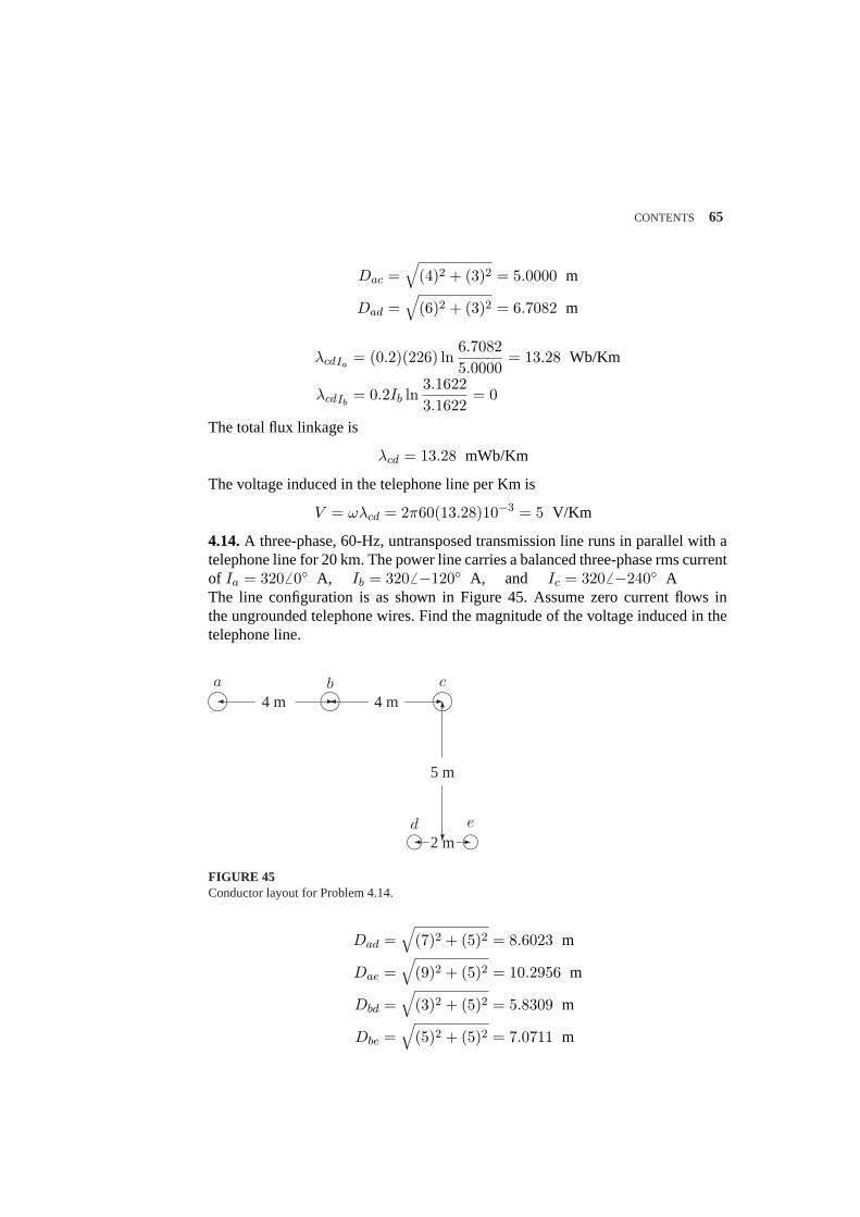
CONTENTS 65
Dac =√
(4)2 + (3)2 = 5.0000 m
Dad =√
(6)2 + (3)2 = 6.7082 m
λcdIa= (0.2)(226) ln
6.70825.0000
= 13.28 Wb/Km
λcdIb= 0.2Ib ln
3.16223.1622
= 0
The total flux linkage is
λcd = 13.28 mWb/Km
The voltage induced in the telephone line per Km is
V = ωλcd = 2π60(13.28)10−3 = 5 V/Km
4.14.A three-phase, 60-Hz, untransposed transmission line runs in parallel with atelephone line for 20 km. The power line carries a balanced three-phase rms currentof Ia = 3206 0 A, Ib = 3206 −120 A, and Ic = 3206 −240 AThe line configuration is as shown in Figure 45. Assume zero current flows inthe ungrounded telephone wires. Find the magnitude of the voltage induced in thetelephone line.
l l l
i i
¾ -¾ -6
?¾ -
4 m 4 m
2 m
5 m
a b c
d e
FIGURE 45Conductor layout for Problem 4.14.
Dad =√
(7)2 + (5)2 = 8.6023 m
Dae =√
(9)2 + (5)2 = 10.2956 m
Dbd =√
(3)2 + (5)2 = 5.8309 m
Dbe =√
(5)2 + (5)2 = 7.0711 m
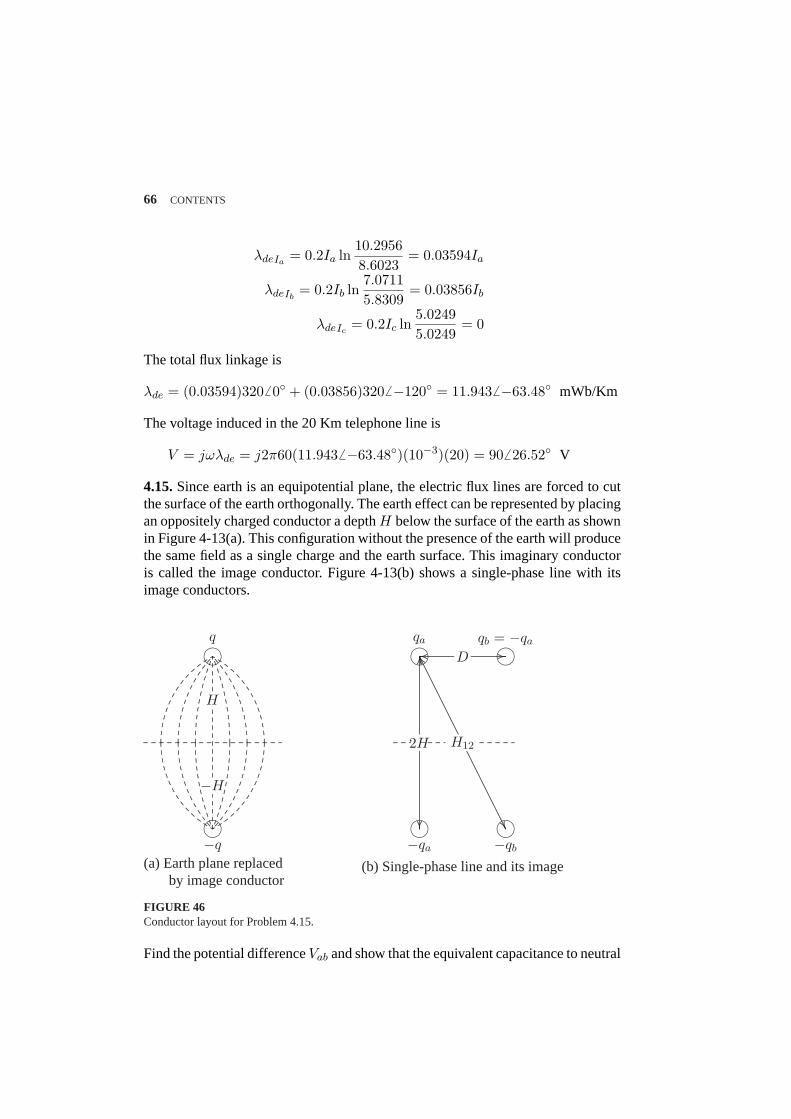
66 CONTENTS
λdeIa= 0.2Ia ln
10.29568.6023
= 0.03594Ia
λdeIb= 0.2Ib ln
7.07115.8309
= 0.03856Ib
λdeIc= 0.2Ic ln
5.02495.0249
= 0
The total flux linkage is
λde = (0.03594)3206 0 + (0.03856)3206 −120 = 11.9436 −63.48 mWb/Km
Thevoltage induced in the 20 Km telephone line is
V = jωλde = j2π60(11.9436 −63.48)(10−3)(20) = 906 26.52 V
4.15.Sinceearth is an equipotential plane, the electric flux lines are forced to cutthe surface of the earth orthogonally. The earth effect can be represented by placingan oppositely charged conductor a depthH below the surface of the earth as shownin Figure 4-13(a). This configuration without the presence of the earth will producethe same field as a single charge and the earth surface. This imaginary conductoris called the image conductor. Figure 4-13(b) shows a single-phase line with itsimage conductors.
l
l
l l
l l
........
........
........
........
........
........
........
........
........
........
........
........
........
........
........
........
........
........
...................
................
...........................................................................................................................................................
........
........
........
....................................................................................................................................................................................................
....................................................................................................................................................................................................
.................................................................................................. .................................................................................. ................
........
................................................................................................ .....
........
........................................................................................
........
........
..........................................................................
........
........................................................................................
.............
........
........................................................................................
........
........
..........................................................................
........
........................................
................
................
................
.............
........
................................................
................
................
........
........
........
..........................................................................
........
.....................................................................................................
........
........................................................................................
........
........
..........................................................................
........ ........ ........ ........ ........ ........ ........ ........ ........ ........ ........ ........ ........ ........ ........ ........ ........ ......
........
........
........
........
......
........
........
........
........
........
........
........
........
........
........
........
........
........
......
........ ........ ... ........ ........ ... ........ ........ ........ ........ ......
q
−q
H
−H
qa qb = −qa
−qa −qb
2H H12
D
(a) Earth plane replacedby image conductor
(b) Single-phase line and its image
FIGURE 46Conductor layout for Problem 4.15.
Find the potential differenceVab and show that the equivalent capacitance to neutral

CONTENTS 67
is given by
Can = Cbn =2πε
ln(
Dr
2HH12
)
Vab =1
2πε
[qa ln
D
r− qa ln
H12
2H+ qb ln
r
D− qb ln
2H
H12
]
Substitutingfor qb = −qa, results in
Vab =qa
πε
[ln
(D
r
2H
H12
)]
Cab =qa
Vab=
πε
ln(
Dr
2HH12
)
Therefore,the equivalent capacitance to neutral is
Can = Cbn = 2Cab =2πε
ln(
Dr
2HH12
)

CHAPTER5 PROBLEMS
5.1.A 69-kV, three-phase short transmission line is 16 km long. The line has a perphase series impedance of0.125 + j0.4375 Ω per km. Determine the sending endvoltage, voltage regulation, the sending end power, and the transmission efficiencywhen the line delivers
(a) 70 MVA, 0.8 lagging power factor at 64 kV.(b) 120 MW, unity power factor at 64 kV.
Uselineperf program to verify your results.
The line impedance is
Z = (0.125 + j0.4375)(16) = 2 + j7 Ω
The receiving end voltage per phase is
VR =646 0√
3= 36.95046 0 kV
(a)The complex power at the receiving end is
SR(3φ) = 706 cos−1 0.8 = 706 36.87 = 56 + j42 MVA
The current per phase is given by
IR =S∗R(3φ)
3V ∗R
=700006 − 36.87
3× 36.95046 0= 631.4776 − 36.87 A
68

CONTENTS 69
Thesending end voltage is
VS = VR + ZIR = 36.95046 0 + (2 + j7)(631.4776 − 36.87)(10−3)= 40.7086 3.9137 kV
Thesending end line-to-line voltage magnitude is
|VS(L−L)| =√
3 |VS | = 70.508 kV
The sending end power is
SS(3φ) = 3VSI∗S = 3× 40.7086 3.9137× 631.4776 36.87 × 10−3
= 58.393 MW + j50.374 Mvar
= 77.11856 40.7837 MVA
Voltage regulation is
PercentV R =70.508− 64
64× 100 = 10.169%
Transmission line efficiency is
η =PR(3φ)
PS(3φ)=
5658.393
× 100 = 95.90%
(b) The complex power at the receiving end is
SR(3φ) = 1206 0 = 120 + j0 MVA
The current per phase is given by
IR =S∗R(3φ)
3V ∗R
=1200006 0
3× 36.95046 0= 1082.536 0 A
Thesending end voltage is
VS = VR + ZIR = 36.95046 0 + (2 + j7)(1082.536 0)(10−3)= 39.84276 10.9639 kV
Thesending end line-to-line voltage magnitude is
|VS(L−L)| =√
3 |VS | = 69.0096 kV

70 CONTENTS
Thesending end power is
SS(3φ) = 3VSI∗S = 3× 39.84276 10.9639× 1082.536 0 × 10−3
= 127.031 MW + j24.609 Mvar
= 129.3936 10.9639 MVA
Voltage regulation is
PercentV R =69.0096− 64
64× 100 = 7.8275%
Transmission line efficiency is
η =PR(3φ)
PS(3φ)=
120127.031
× 100 = 94.465%
The above computations are performed efficiently using thelineperf program.
The command:
lineperf
displays the following menu
Type of parameters for input SelectParameters per unit lengthr (Ω), g (Siemens), L (mH), C (µF) 1
Complex z and y per unit lengthr + j*x (Ω), g + j*b (Siemens) 2
Nominal π or Eq. π model 3
A, B, C, D constants 4
Conductor configuration and dimension 5
To quit 0Select number of menu → 2Enter line length = 16Enter frequency in Hz = 60Enter series impedance r + j*x in ohm per unit lengthz = 0.125+j*0.4375Enter shunt admittance g + j*b in siemens per unit lengthy = 0+j*0

CONTENTS 71
Short line modelZ = 2 + j 7 ohms
ABCD =[
1 + j0 2 + j70 + j0 1 + j0
]
Transmission line performanceAnalysis Select
To calculate sending end quantitiesfor specified receiving end MW, Mvar 1
To calculate receiving end quantitiesfor specified sending end MW, Mvar 2
To calculate sending end quantitieswhen load impedance is specified 3
Open-end line and reactive compensation 4
Short-circuited line 5
Capacitive compensation 6
Receiving end circle diagram 7
Loadability curve and voltage profile 8
To quit 0
Select number of menu → 1
Enter receiving end line-line voltage kV = 64Enter receiving end voltage phase angle = 0Enter receiving end 3-phase power MW = 56Enter receiving end 3-phase reactive power(+ for lagging and - for leading power factor) Mvar = 42
Line performance for specified receiving end quantities
Vr = 64 kV (L-L) at 0Pr = 56 MW Qr = 42 Mvar

72 CONTENTS
Ir = 631.477 A at -36.8699 PFr = 0.8 laggingVs = 70.5082 kV (L-L) at 3.91374Is = 631.477 A at -36.8699 PFs = 0.757182 laggingPs = 58.393 MW Qs = 50.374 MvarPL = 2.393 MW QL = 8.374 MvarPercent Voltage Regulation = 10.169Transmission line efficiency = 95.9026
At the end of this analysis thelistmenu (Analysis Menu) is displayed. Selectingoption 1 and entering data for part (b), will result in
Line performance for specified receiving end quantities
Vr = 64 kV (L-L) at 0Pr = 120 MW Qr = 0 MvarIr = 1082.53 A at 0 PFr = 1Vs = 69.0096 kV (L-L) at 10.9639Is = 1082.53 A at 0 PFs = 0.981747Ps = 127.031 MW Qs = 24.069 MvarPL = 7.031 MW QL = 24.069 MvarPercent Voltage Regulation = 7.82754Transmission line efficiency = 94.4649
5.2.Shunt capacitors are installed at the receiving end to improve the line perfor-mance of Problem 5.1. The line delivers 70 MVA, 0.8 lagging power factor at 64kV. Determine the total Mvar and the capacitance per phase of the Y-connectedcapacitors when the sending end voltage is
(a) 69 kV.(b) 64 kV.
Hint: Use (5.85) and (5.86) to compute the power angleδ and the receivingend reactive power.(c) Uselineperf to obtain the compensated line performance.
The complex load at the receiving end is
SR(3φ) = 70 6 cos−1 0.8 = 56 MW + j42 Mvar
Z = 2 + j7 = 7.286 74.0546
(a)ForVR(LL) = 69 kV, from (5.85), we have
56 =(69)(64)
7.28cos(74.0564− δ)− (1.0)(64)2
7.28cos 74.0546

CONTENTS 73
Therefore,
cos(74.0546− δ) = 0.3471 or δ = 4.3646
Now from (5.86), we have
QR(3φ) =(69)(64)
7.28sin(74.0564− 4.3646)− (1.0)(64)2
7.28sin 74.0546
= 27.883 Mvar
Therefore, the required capacitor Mvar is
QC = 42− 27.883 = 14.117 Mvar
ZC =|VR|2S∗C
=(64/sqrt3)2
j14.117/3= −j290.147 Ω
The required shunt capacitance per phase is
C =106
(2π)(60)(290.147)= 9.1422 µF
(b) ForVR(LL) = 64 kV, from (5.85), we have
56 =(64)(64)
7.28cos(74.0564− δ)− (1.0)(64)2
7.28cos 74.0546
Therefore,
cos(74.0546− δ) = 0.37425 or δ = 6.0327
Now from (5.86), we have
QR(3φ) =(64)(64)
7.28sin(74.0564− 6.0327)− (1.0)(64)2
7.28sin 74.0546
= − 19.2405 Mvar
Therefore, the required capacitor Mvar is
QC = 42− (−19.2405) = 61.2405 Mvar
ZC =|VR|2S∗C
=(64/sqrt3)2
j61.2405/3= −j66.8838 Ω
The required shunt capacitance per phase is
C =106
(2π)(60)(66.8838)= 39.6596 µF
With lineperf program, we continue the analysis in Problem 5.1 by selecting option6. This will display thecompmenu

74 CONTENTS
Capacitive compensationAnalysis Select
Shunt capacitive compensation 1
Series capacitive compensation 2
Series and shunt capacitive compensation 3
To quit 0
Selecting option 1 of thecompmenuresults in
Enter sending end line-line voltage kV = 69Enter desired receiving end line-line voltage kV = 64Enter receiving end voltage phase angle = 0Enter receiving end 3-phase power MW = 56Enter receiving end 3-phase reactive power(+ for lagging and - for leading power factor) Mvar = 42
Shunt capacitive compensation
Vs = 69 kV (L-L) at 4.36672Vr = 64 kV (L-L) at 0Pload = 56 MW, Qload = 42 MvarLoad current = 631.477 A at -36.8699, PFl = 0.8 laggingRequired shunt capacitor: 290.147 Ω, 9.14222 µF, 14.117 MvarShunt capacitor current = 127.351 A at 90Pr = 56.000 MW, Qr = 27.883 MvarIr = 564.339 A at -26.4692, PFr = 0.895174 laggingIs = 564.339 A at -26.4692 PFs = 0.858639 laggingPs = 57.911 MW, Qs = 34.571 MvarPL = 1.911 MW, QL = 6.688 MvarPercent Voltage Regulation = 7.8125Transmission line efficiency = 96.7003
Repeating for part (b), we have
Shunt capacitive compensation
Vs = 64 KV (L-L) at 6.03281Vr = 64 KV (L-L) at 0Pload = 56 MW, Qload = 42 MvarLoad current = 631.477 A at -36.8699, PFl = 0.8 laggingRequired shunt capacitor: 66.8837Ω, 39.6596 µF, 61.2406 Mvar

CONTENTS 75
Shunt capacitor current = 552.457 A at 90Pr = 56.000 MW, Qr = -19.241 MvarIr = 534.168 A at 18.9618, PFr = 0.945735 leadingIs = 534.168 A at 18.9618 PFs = 0.974648 leadingPs = 57.712 MW, Qs = -13.249 MvarPL = 1.712 MW, QL = 5.992 MvarPercent Voltage Regulation = 2.22045e-14Transmission line efficiency = 97.0335
5.3.A 230-kV, three-phase transmission line has a per phase series impedance ofz = 0.05 + j0.45 Ω per Km and a per phase shunt admittance ofy = j3.4× 10−6
siemens per km. The line is 80 km long. Using the nominalπ model, determine
(a) The transmission line ABCD constants. Find the sending end voltage and cur-rent, voltage regulation, the sending end power and the transmission efficiencywhen the line delivers(b) 200 MVA, 0.8 lagging power factor at 220 kV.(c) 306 MW, unity power factor at 220 kV.
Uselineperf program to verify your results.
The line impedance and shunt admittance are
Z = (0.05 + j0.45)(80) = 4 + j36 Ω
Y = (j3.4× 10−6)(80) = j0.272× 10−3 siemens
The ABCD constants of the nominalπ model are
A = (1 +ZY
2) = (1 +
(4 + j36)(j0.272× 10−3)2
) = 0.9951 + j0.000544
B = Z = 4 + j36
C = Y (1 +ZY
4) = j0.0002713
The receiving end voltage per phase is
VR =2206 0√
3= 1276 0 kV
(a)The complex power at the receiving end is
SR(3φ) = 2006 cos−1 0.8 = 2006 36.87 = 160 + j120 MVA

76 CONTENTS
Thecurrent per phase is given by
IR =S∗R(3φ)
3V ∗R
=2000006 − 36.87
3× 1276 0= 524.8646 − 36.87 A
Thesending end voltage is
VS = AVR + BIR = 0.9951 + j0.000544)(1276 0) + (4 + j36)(524.864× 10⁻³ 6 −36.87) = 140.10516 5.704 kV
Thesending end line-to-line voltage magnitude is
|VS(L−L)| =√
3 |VS | = 242.67 kV
The sending end current is
IS = CVR + DIR = (j0.0002713)(1270006 0) + (0.9951 + j0.000544)(524.8646 −36.87) = 502.386 −33.69 A
Thesending end power is
SS(3φ) = 3VSI∗S = 3× 140.10516 5.704× 502.386 33.69 × 10−3
= 163.179 MW + j134.018 Mvar
= 211.166 39.396 MVA
Voltage regulation is
PercentV R =242.670.9951 − 220
220× 100 = 10.847%
Transmission line efficiency is
η =PR(3φ)
PS(3φ)=
160163.179
× 100 = 98.052%
(b) The complex power at the receiving end is
SR(3φ) = 3066 0 = 306 + j0 MVA
The current per phase is given by
IR =S∗R(3φ)
3V ∗R
=3060006 0
3× 1276 0= 803.4026 0 A

CONTENTS 77
Thesending end voltage is
VS = AVR + BIR = 0.9951 + j0.000544)(1276 0) + (4 + j36)(803.402× 10⁻³ 6 0) = 132.8076 12.6 kV
Thesending end line-to-line voltage magnitude is
|VS(L−L)| =√
3 |VS | = 230.029 kV
The sending end current is
IS = CVR + DIR = (j0.0002713)(1270006 0) + (0.9951 + j0.000544)(803.4026 0) = 799.8626 2.5 A
Thesending end power is
SS(3φ) = 3VSI∗S = 3× 132.8076 12.6× 799.8626 − 2.5 × 10−3
= 313.742 MW + j55.9 Mvar
= 318.686 10.1 MVA
Voltage regulation is
PercentV R =230.0290.9951 − 220
220× 100 = 5.073%
Transmission line efficiency is
η =PR(3φ)
PS(3φ)=
306313.742
× 100 = 97.53%
The above computations are performed efficiently using thelineperf program.The command:
lineperf
displays the following menu
Type of parameters for input SelectParameters per unit lengthr (Ω), g (Siemens), L (mH), C (µF) 1
Complex z and y per unit lengthr + j*x (Ω), g + j*b (Siemens) 2

78 CONTENTS
Nominal π or Eq. π model 3
A, B, C, D constants 4
Conductor configuration and dimension 5
To quit 0Select number of menu → 2Enter line length = 80Enter frequency in Hz = 60Enter series impedance r + j*x in ohm per unit length z =0.05 + j0.45Enter shunt admittance g + j*b in siemens per unit length y =0+j*3.4e-6
Short line modelZ = 4 + j 36 ohmsY = 0 + j 0.000272 Siemens
ABCD =[
0.9951 + j0.000544 4 + j36−7.3984e− 008 + j0.00027133 0.9951 + j0.000544
]
Transmission line performanceAnalysis Select
To calculate sending end quantitiesfor specified receiving end MW, Mvar 1
To calculate receiving end quantitiesfor specified sending end MW, Mvar 2
To calculate sending end quantitieswhen load impedance is specified 3
Open-end line and reactive compensation 4
Short-circuited line 5
Capacitive compensation 6

CONTENTS 79
Receiving end circle diagram 7
Loadability curve and voltage profile 8
To quit 0
Select number of menu → 1
Enter receiving end line-line voltage kV = 220Enter receiving end voltage phase angle = 0Enter receiving end 3-phase power MW = 160Enter receiving end 3-phase reactive power(+ for lagging and - for leading power factor) Mvar = 120
Line performance for specified receiving end quantities
Vr = 220 kV (L-L) at 0Pr = 160 MW Qr = 120 MvarIr = 524.864 A at -36.8699 PFr = 0.8 laggingVs = 242.67 kV (L-L) at 5.7042Is = 502.381 A at -33.6919 PFs = 0.77277 laggingPs = 163.179 MW Qs = 134.018 MvarPL = 3.179 MW QL = 14.018 MvarPercent Voltage Regulation = 10.847Transmission line efficiency = 98.052
At the end of this analysis thelistmenu (Analysis Menu) is displayed. Selectingoption 1 and entering data for part (b), will result in
Line performance for specified receiving end quantities
Vr = 220 kV (L-L) at 0Pr = 306 MW Qr = 0 MvarIr = 803.042 A at 0 PFr = 1Vs = 230.029 kV (L-L) at 12.6033Is = 799.862 A at 2.5008 PFs = 0.984495Ps = 313.742 MW Qs = 55.900 MvarPL = 7.742 MW QL = 55.900 MvarPercent Voltage Regulation = 5.0732Transmission line efficiency = 97.532
5.4.Shunt capacitors are installed at the receiving end to improve the line perfor-mance of Problem 5.3. The line delivers 200 MVA, 0.8 lagging power factor at 220kV.
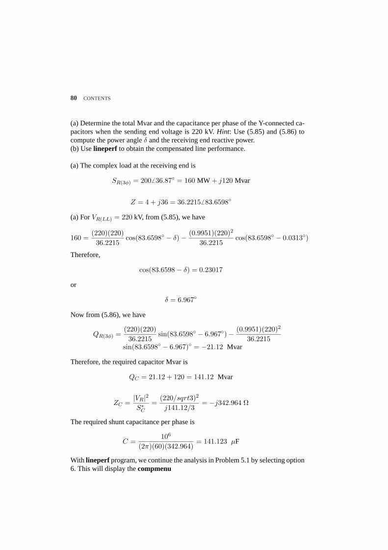
80 CONTENTS
(a)Determine the total Mvar and the capacitance per phase of the Y-connected ca-pacitors when the sending end voltage is 220 kV.Hint: Use (5.85) and (5.86) tocompute the power angleδ and the receiving end reactive power.(b) Uselineperf to obtain the compensated line performance.
(a) The complex load at the receiving end is
SR(3φ) = 2006 36.87 = 160 MW + j120 Mvar
Z = 4 + j36 = 36.22156 83.6598
(a)ForVR(LL) = 220 kV, from (5.85), we have
160 =(220)(220)36.2215
cos(83.6598 − δ)− (0.9951)(220)2
36.2215cos(83.6598 − 0.0313)
Therefore,
cos(83.6598− δ) = 0.23017
or
δ = 6.967
Now from (5.86), we have
QR(3φ) =(220)(220)36.2215
sin(83.6598 − 6.967)− (0.9951)(220)2
36.2215sin(83.6598 − 6.967) = −21.12 Mvar
Therefore, the required capacitor Mvar is
QC = 21.12 + 120 = 141.12 Mvar
ZC =|VR|2S∗C
=(220/sqrt3)2
j141.12/3= −j342.964 Ω
The required shunt capacitance per phase is
C =106
(2π)(60)(342.964)= 141.123 µF
With lineperf program, we continue the analysis in Problem 5.1 by selecting option6. This will display thecompmenu

CONTENTS 81
Capacitive compensationAnalysis Select
Shunt capacitive compensation 1
Series capacitive compensation 2
Series and shunt capacitive compensation 3
To quit 0
Selecting option 1 of thecompmenuresults in
Enter sending end line-line voltage kV = 220Enter desired receiving end line-line voltage kV = 220Enter receiving end voltage phase angle = 0Enter receiving end 3-phase power MW = 160Enter receiving end 3-phase reactive power(+ for lagging and - for leading power factor) Mvar = 120
Shunt capacitive compensation
Vs = 220 kV (L-L) at 6.96702Vr = 220 kV (L-L) at 0Pload = 160 MW, Qload = 120 MvarLoad current = 524.864 A at -36.8699, PFl = 0.8 laggingRequired shunt capacitor: 342.964 Ω, 7.73428 µF, 141.123 MvarShunt capacitor current = 370.351 A at 90Pr = 160.000 MW, Qr = -21.123 MvarIr = 423.534 A at 7.52047, PFr = 0.991398 leadingIs = 427.349 A at 12.1375 PFs = 0.995931 leadingPs = 162.179 MW, Qs = -14.675 MvarPL = 2.179 MW, QL = 6.447 MvarPercent Voltage Regulation = 0.49199Transmission line efficiency = 98.6563
5.5. A three-phase, 345-kV, 60-Hz transposed line is composed of two ACSR1,113,000, 45/7 Bluejay conductors per phase with flat horizontal spacing of 11 m.The conductors have a diameter of 3.195 cm and aGMR of 1.268 cm. The bundlespacing is 45 cm. The resistance of each conductor in the bundle is0.0538 Ω perkm and the line conductance is negligible. The line is 150 Km long. Using the nom-inal π model, determine the ABCD constant of the line. Uselineperf and option 5to verify your results.
GMD = 3
√(11)(11)(22) = 13.859 m

82 CONTENTS
GMRL =√
(45)(1.268) = 7.5538 cm
GMRC =√
(45)(3.195/2) = 8.47865 cm
L = 0.213.859
7.5538× 10−2= 1.0424 mH/Km
C =0.0556
ln 13.8598.47865×10−2
= 0.010909 µF/Km
Z = (0.0538
2+ j2π × 60× 1.0424× 10−3)(150) = 4.035 + j58.947
Y = j(2π60× 0.9109× 10−6)(150) = j0.0006169
The ABCD constants of the nominalπ model are
A =(
1 +ZY
2
)=
(1 +
(4.035 + j38.947)(j0.0006169)2
)
= 0.98182 + j0.0012447B = Z = 4.035 + j58.947
C = Y
(1 +
ZY
4
)= j0.00061137
Using lineperf andoption 5, result in
Type of parameters for input SelectParameters per unit lengthr (Ω), g (Siemens), L (mH), C (µF) 1
Complex z and y per unit lengthr + j*x (Ω), g + j*b (Siemens) 2
Nominal π or Eq. π model 3
A, B, C, D constants 4
Conductor configuration and dimension 5
To quit 0
Select number of menu → 5

CONTENTS 83
Whenthe line configuration and conductor specifications are entered, the followingresults are obtained
GMD = 13.85913 mGMRL = 0.07554 m GMRC = 0.08479 mL = 1.04241 mH/Km C = 0.0109105 micro F/Km
Short line modelZ = 4.035 + j 58.947 ohmsY = 0 + j 0.000616976 Siemens
ABCD =[
0.98182 + j0.0012447 4.035 + j58.947−3.8399e− 007 + j0.00061137 0.98182 + j0.0012447
]
5.6.The ABCD constants of a three-phase, 345-kV transmission line are
A = D = 0.98182 + j0.0012447B = 4.035 + j58.947C = j0.00061137
The line delivers 400 MVA at 0.8 lagging power factor at 345 kV. Determine thesending end quantities, voltage regulation, and transmission efficiency.
The receiving end voltage per phase is
VR =3456 0√
3= 199.1866 0 kV
(a)The complex power at the receiving end is
SR(3φ) = 4006 cos−1 0.8 = 4006 36.87 = 320 + j240 MVA
The current per phase is given by
IR =S∗R(3φ)
3V ∗R
=4000006 − 36.87
3× 199.1866 0= 669.3926 − 36.87 A
Thesending end voltage is
VS = AVR + BIR = 0.98182 + j0.0012447)(199.1866 0) + (4.035 + j58.947)(668.392× 10⁻³ 6 −36.87) = 223.4496 7.766 kV

84 CONTENTS
Thesending end line-to-line voltage magnitude is
|VS(L−L)| =√
3 |VS | = 387.025 kV
The sending end current is
IS = CVR + DIR = (j0.00061137)(199.1866 0) + (0.98182 + j0.0012447)(669.3926 −36.87) = 592.2916 −27.3256 A
Thesending end power is
SS(3φ) = 3VSI∗S = 3× 223.4496 7.766× 592.2916 27.3256 × 10−3
= 324.872 MW + j228.253 Mvar
= 397.0416 35.0916 MVA
Voltage regulation is
PercentV R =387.0250.98182 − 345
345× 100 = 14.2589%
Transmission line efficiency is
η =PR(3φ)
PS(3φ)=
320324.872
× 100 = 98.500%
Using lineperf and option 4, result in
Select number of menu → 4Enter the complex constant A = 0.98182+j*0.0012447Enter the complex constant B = 4.035+j*58.947Enter the complex constant C = j*0.00061137Two port model, ABCD constantsZ = 4.035 + j 58.947 ohmY = 3.87499e-007 + j 0.000616978 siemens
ABCD =[
0.98182 + j0.0012447 4.035 + j58.9470 + j0.00061137 0.98182 + j0.0012447
]
Transmission line performanceAnalysis Select
To calculate sending end quantitiesfor specified receiving end MW, Mvar 1
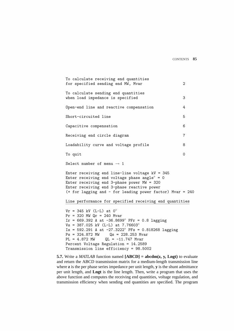
CONTENTS 85
To calculate receiving end quantitiesfor specified sending end MW, Mvar 2
To calculate sending end quantitieswhen load impedance is specified 3
Open-end line and reactive compensation 4
Short-circuited line 5
Capacitive compensation 6
Receiving end circle diagram 7
Loadability curve and voltage profile 8
To quit 0
Select number of menu → 1
Enter receiving end line-line voltage kV = 345Enter receiving end voltage phase angle = 0Enter receiving end 3-phase power MW = 320Enter receiving end 3-phase reactive power(+ for lagging and - for leading power factor) Mvar = 240
Line performance for specified receiving end quantities
Vr = 345 kV (L-L) at 0Pr = 320 MW Qr = 240 MvarIr = 669.392 A at -36.8699 PFr = 0.8 laggingVs = 387.025 kV (L-L) at 7.76603Is = 592.291 A at -27.3222 PFs = 0.818268 laggingPs = 324.872 MW Qs = 228.253 MvarPL = 4.872 MW QL = -11.747 MvarPercent Voltage Regulation = 14.2589Transmission line efficiency = 98.5002
5.7. Write a MATLAB function named[ABCD] = abcdm(z, y, Lngt) to evaluateand return the ABCD transmission matrix for a medium-length transmission linewherez is the per phase series impedance per unit length,y is the shunt admittanceper unit length, andLngt is the line length. Then, write a program that uses theabove function and computes the receiving end quantities, voltage regulation, andtransmission efficiency when sending end quantities are specified. The program

86 CONTENTS
shouldprompt the user to enter the following quantities:
The sending end line-to-line voltage magnitude in kVThe sending end voltage phase angle in degreesThe three-phase sending end real power in MWThe three-phase sending end reactive power in Mvar
Use your program to obtain the solution for the following case:
A three-phase transmission line has a per phase series impedance ofz = 0.03 +j0.4 Ω per Km and a per phase shunt admittance ofy = j4.0× 10−6 siemens perKm. The line is 125 Km long. Obtain the ABCD transmission matrix. Determinethe receiving end quantities, voltage regulation, and the transmission efficiencywhen the line is sending 407 MW, 7.833 Mvar at 350 kV.
The following function namedabcdm returns the line ABCD constants
function [ABCD] = abcdm(z, y, Lngt);Z = z*Lngt;Y = y*Lngt;A = 1 + Z*Y/2; B = Z;C = Y*(1 + Z*Y/4); D = A;ABCD = [A B; C D];
The following program saved asch5p7.mcomputes the receiving end quantitiesfrom the specified sending end quantities.
z=input(’Line series impedance per phase per unit length z=’);y=input(’Line shunt admittance per phase per unit length y=’);Lngt = input(’Transmission line length = ’);ABCD = abcdm(z, y,Lngt)VL_s=input(’Sending end line-to-line voltage magnitude in kV=’);AngV_s=input(’Sending end voltage phase angle in degree = ’);P_s =input(’Three-phase sending end real power in MW ’);Q_s =input(’Three-phase sending end reactive power in Mvar ’);S_s = P_s + j*Q_s; % MVAAngV_srd = AngV_s*pi/180; % RadianV_s = VL_s/sqrt(3)*(cos(AngV_srd) + j*sin(AngV_srd)); %kVI_s = conj(S_s)/(3*conj(V_s)); % kAIL_s= abs(I_s)*1000; AngI_srd = angle(I_s);AngI_s = AngI_srd*180/pi;VI_r = inv(ABCD)*[V_s; I_s];V_r = VI_r(1); VL_r = sqrt(3)*abs(V_r);AngV_rrd = angle(V_r); AngV_r = AngV_rrd*180/pi;
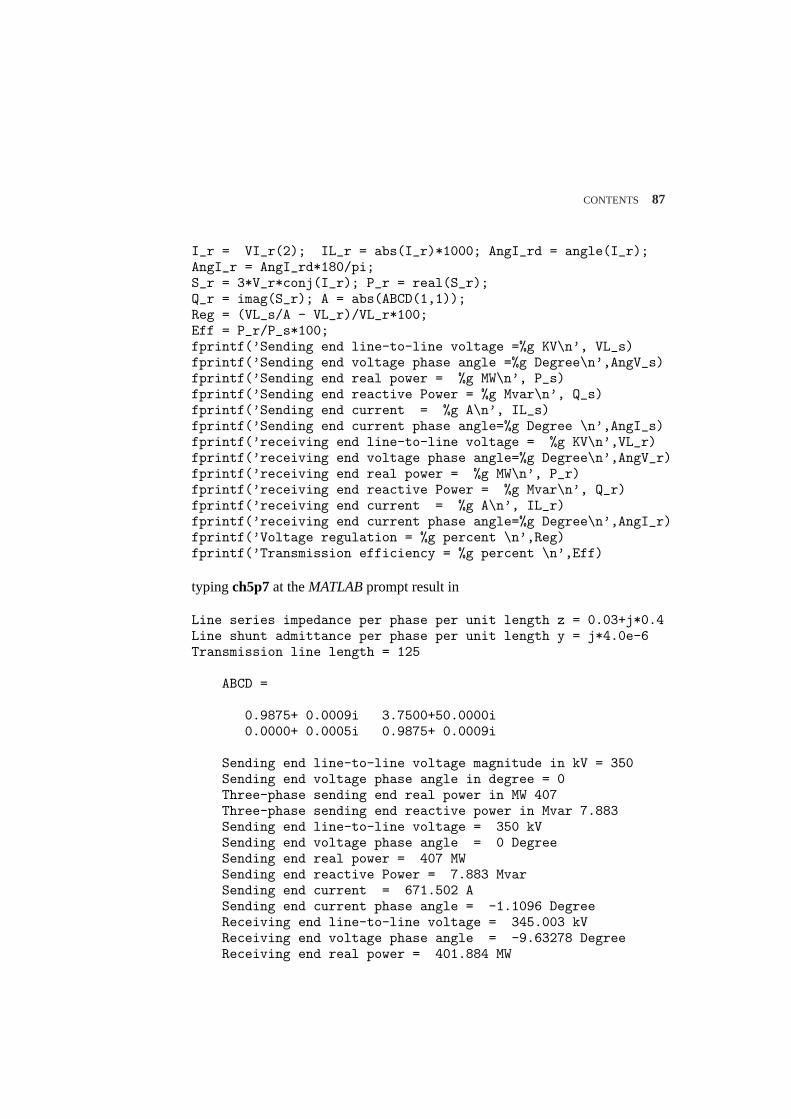
CONTENTS 87
I_r = VI_r(2); IL_r = abs(I_r)*1000; AngI_rd = angle(I_r);AngI_r = AngI_rd*180/pi;S_r = 3*V_r*conj(I_r); P_r = real(S_r);Q_r = imag(S_r); A = abs(ABCD(1,1));Reg = (VL_s/A - VL_r)/VL_r*100;Eff = P_r/P_s*100;fprintf(’Sending end line-to-line voltage =%g KV\n’, VL_s)fprintf(’Sending end voltage phase angle =%g Degree\n’,AngV_s)fprintf(’Sending end real power = %g MW\n’, P_s)fprintf(’Sending end reactive Power = %g Mvar\n’, Q_s)fprintf(’Sending end current = %g A\n’, IL_s)fprintf(’Sending end current phase angle=%g Degree \n’,AngI_s)fprintf(’receiving end line-to-line voltage = %g KV\n’,VL_r)fprintf(’receiving end voltage phase angle=%g Degree\n’,AngV_r)fprintf(’receiving end real power = %g MW\n’, P_r)fprintf(’receiving end reactive Power = %g Mvar\n’, Q_r)fprintf(’receiving end current = %g A\n’, IL_r)fprintf(’receiving end current phase angle=%g Degree\n’,AngI_r)fprintf(’Voltage regulation = %g percent \n’,Reg)fprintf(’Transmission efficiency = %g percent \n’,Eff)
typingch5p7at theMATLABprompt result in
Line series impedance per phase per unit length z = 0.03+j*0.4Line shunt admittance per phase per unit length y = j*4.0e-6Transmission line length = 125
ABCD =
0.9875+ 0.0009i 3.7500+50.0000i0.0000+ 0.0005i 0.9875+ 0.0009i
Sending end line-to-line voltage magnitude in kV = 350Sending end voltage phase angle in degree = 0Three-phase sending end real power in MW 407Three-phase sending end reactive power in Mvar 7.883Sending end line-to-line voltage = 350 kVSending end voltage phase angle = 0 DegreeSending end real power = 407 MWSending end reactive Power = 7.883 MvarSending end current = 671.502 ASending end current phase angle = -1.1096 DegreeReceiving end line-to-line voltage = 345.003 kVReceiving end voltage phase angle = -9.63278 DegreeReceiving end real power = 401.884 MW
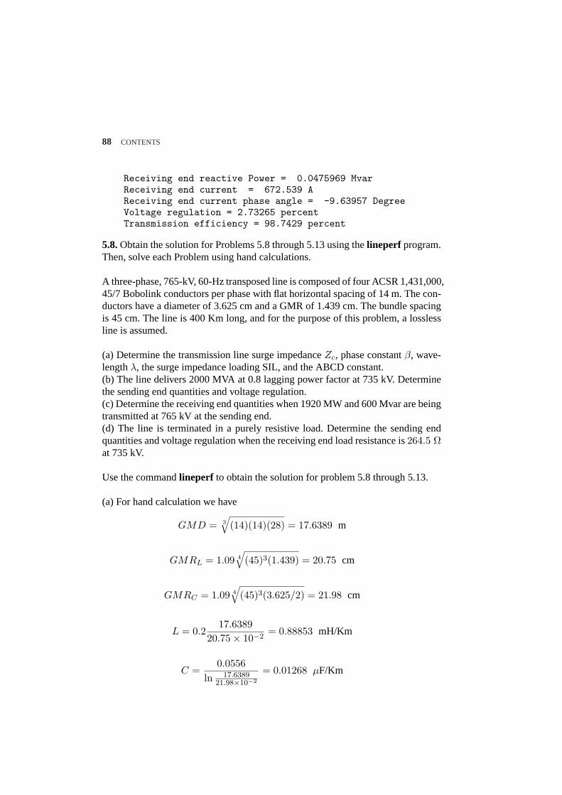
88 CONTENTS
Receiving end reactive Power = 0.0475969 MvarReceiving end current = 672.539 AReceiving end current phase angle = -9.63957 DegreeVoltage regulation = 2.73265 percentTransmission efficiency = 98.7429 percent
5.8.Obtain the solution for Problems 5.8 through 5.13 using thelineperf program.Then, solve each Problem using hand calculations.
A three-phase, 765-kV, 60-Hz transposed line is composed of four ACSR 1,431,000,45/7 Bobolink conductors per phase with flat horizontal spacing of 14 m. The con-ductors have a diameter of 3.625 cm and a GMR of 1.439 cm. The bundle spacingis 45 cm. The line is 400 Km long, and for the purpose of this problem, a losslessline is assumed.
(a) Determine the transmission line surge impedanceZc, phase constantβ, wave-lengthλ, the surge impedance loading SIL, and the ABCD constant.(b) The line delivers 2000 MVA at 0.8 lagging power factor at 735 kV. Determinethe sending end quantities and voltage regulation.(c) Determine the receiving end quantities when 1920 MW and 600 Mvar are beingtransmitted at 765 kV at the sending end.(d) The line is terminated in a purely resistive load. Determine the sending endquantities and voltage regulation when the receiving end load resistance is264.5 Ωat 735 kV.
Use the commandlineperf to obtain the solution for problem 5.8 through 5.13.
(a) For hand calculation we have
GMD = 3
√(14)(14)(28) = 17.6389 m
GMRL = 1.09 4
√(45)3(1.439) = 20.75 cm
GMRC = 1.09 4
√(45)3(3.625/2) = 21.98 cm
L = 0.217.6389
20.75× 10−2= 0.88853 mH/Km
C =0.0556
ln 17.638921.98×10−2
= 0.01268 µF/Km
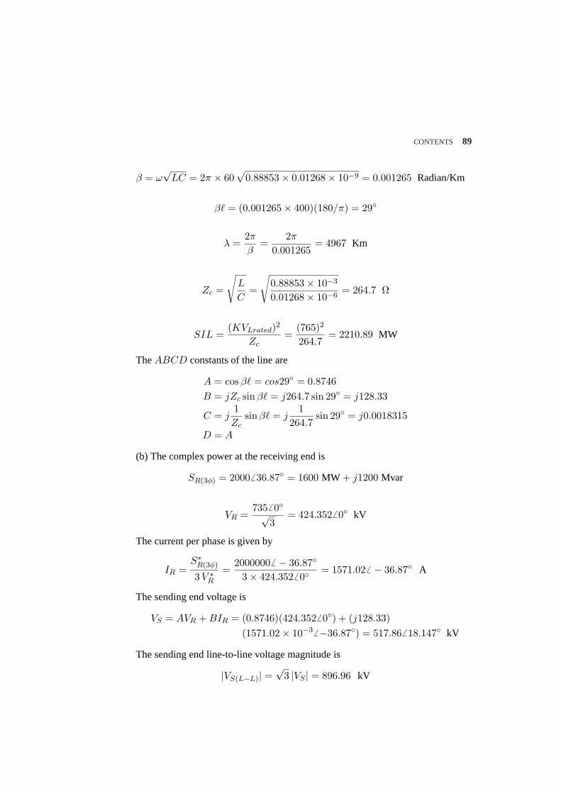
CONTENTS 89
β = ω√
LC = 2π × 60√
0.88853× 0.01268× 10−9 = 0.001265 Radian/Km
β` = (0.001265× 400)(180/π) = 29
λ =2π
β=
2π
0.001265= 4967 Km
Zc =
√L
C=
√0.88853× 10⁻³
0.01268× 10−6= 264.7 Ω
SIL =(KVLrated)2
Zc=
(765)2
264.7= 2210.89 MW
TheABCD constants of the line are
A = cos β` = cos29 = 0.8746B = jZc sinβ` = j264.7 sin 29 = j128.33
C = j1Zc
sinβ` = j1
264.7sin 29 = j0.0018315
D = A
(b) The complex power at the receiving end is
SR(3φ) = 20006 36.87 = 1600 MW + j1200 Mvar
VR =7356 0√
3= 424.3526 0 kV
Thecurrent per phase is given by
IR =S∗R(3φ)
3V ∗R
=20000006 − 36.87
3× 424.3526 0= 1571.026 − 36.87 A
Thesending end voltage is
VS = AVR + BIR = (0.8746)(424.3526 0) + (j128.33)(1571.02× 10−3 6 −36.87) = 517.866 18.147 kV
Thesending end line-to-line voltage magnitude is
|VS(L−L)| =√
3 |VS | = 896.96 kV
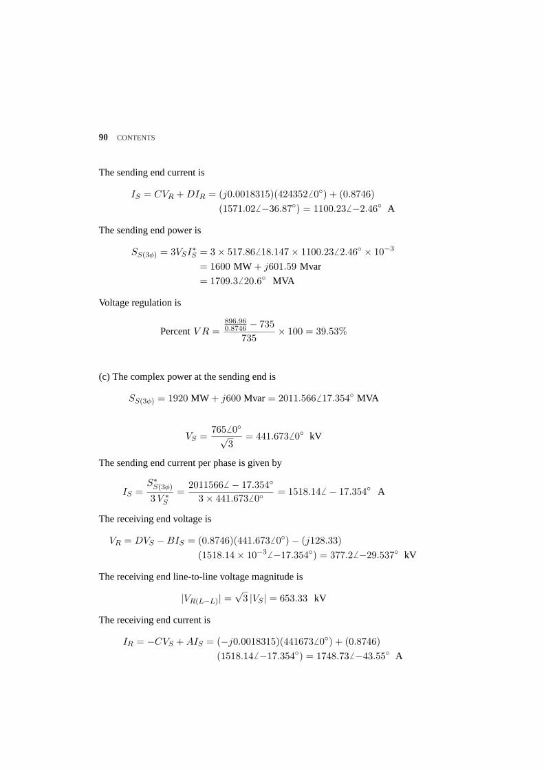
90 CONTENTS
Thesending end current is
IS = CVR + DIR = (j0.0018315)(4243526 0) + (0.8746)(1571.026 −36.87) = 1100.236 −2.46 A
Thesending end power is
SS(3φ) = 3VSI∗S = 3× 517.866 18.147× 1100.236 2.46 × 10−3
= 1600 MW + j601.59 Mvar
= 1709.36 20.6 MVA
Voltage regulation is
PercentV R =896.960.8746 − 735
735× 100 = 39.53%
(c) The complex power at the sending end is
SS(3φ) = 1920 MW + j600 Mvar = 2011.5666 17.354 MVA
VS =7656 0√
3= 441.6736 0 kV
Thesending end current per phase is given by
IS =S∗S(3φ)
3V ∗S
=20115666 − 17.354
3× 441.6736 0= 1518.146 − 17.354 A
Thereceiving end voltage is
VR = DVS −BIS = (0.8746)(441.6736 0)− (j128.33)(1518.14× 10−3 6 −17.354) = 377.26 −29.537 kV
Thereceiving end line-to-line voltage magnitude is
|VR(L−L)| =√
3 |VS | = 653.33 kV
The receiving end current is
IR = −CVS + AIS = (−j0.0018315)(4416736 0) + (0.8746)(1518.146 −17.354) = 1748.736 −43.55 A

CONTENTS 91
Thereceiving end power is
SR(3φ) = 3VRI∗R = 3× 377.26 − 29.537 × 1748.736 43.55 × 10−3
= 1920 MW + j479.2 Mvar
= 1978.866 14.013 MVA
Voltage regulation is
PercentV R =765
0.8746 − 653.33653.33
× 100 = 33.88%
(d)
VR =7356 0√
3= 424.3526 0 kV
Thereceiving end current per phase is given by
IR =VR
ZL=
4243526 0
264.5= 1604.3576 0 A
Thecomplex power at the receiving end is
SR(3φ) = 3VRIR∗ = 3(424.3526 0)(1604.3576 0)× 10−3 = 2042.44 MW
The sending end voltage is
VS = AVR + BIR = (0.8746)(424.3526 0) + (j128.33)= (1604.357× 10−3 6 0) = 424.426 29.02 kV
Thesending end line-to-line voltage magnitude is
|VS(L−L)| =√
3 |VS | = 735.12 kV
The sending end current is
IS = CVR + DIR = (j0.0018315)(4243526 0) + (0.8746)(1604.3576 0) = 1604.046 28.98 A
Thesending end power is
SS(3φ) = 3VSI∗S = 3× 424.426 29.02× 1604.046 − 28.98 × 10−3
= 2042.4 MW + j1.4 Mvar
= 2042.366 0.04 MVA

92 CONTENTS
Voltage regulation is
PercentV R =735.120.8746 − 735
735× 100 = 14.36%
5.9.The transmission line of Problem 5.8 is energized with 765 kV at the sendingend when the load at the receiving end is removed.
(a) Find the receiving end voltage.(b) Determine the reactance and the Mvar of a three-phase shunt reactor to beinstalled at the receiving end in order to limit the no-load receiving end voltage to735 kV.(a) The sending end voltage per phase is
VS =7656 0√
3= 441.6736 0 kV
Whenline is openIR = 0 and from (5.71) the no-load receiving end voltage isgiven by
VR(nl) =VS
cosβ`=
441.6730.8746
= 505 kV
The no-load receiving end line-to-line voltage is
VR(L−L)(nl) =√
3VR(nl) = 874.68 kV
(b) ForVRLL = 735 kV, the required inductor reactance given by (5.100) is
XLsh =sin(29)
765735 − cos(29)
(264.7) = 772.13 Ω
The three-phase shunt reactor rating is
Q3φ =(KVLrated)2
XLsh=
(735)2
772.13= 699.65 Mvar
5.10.The transmission line of Problem 5.8 is energized with 765 kV at the sendingend when a three-phase short-circuit occurs at the receiving end. Determine thereceiving end current and the sending end current.
For a solid short at the receiving end,VR = 0 and from (5.71) and (5.72) we have
Vs = jZc sinβ`IR

CONTENTS 93
or
IR =765000/
√3
j264.7 sin 29= 3441.76 − 90 A
IS = cosβ`IR = (cos 29)(3441.7 6 − 90) = 30106 − 90 A
5.11.Shuntcapacitors are installed at the receiving end to improve the line per-formance of Problem 5.8. The line delivers 2000 MVA, 0.8 lagging power factor.Determine the total Mvar and the capacitance per phase of the Y-connected capac-itors to keep the receiving end voltage at 735 kV when the sending end voltage is765 kV.Hint: Use (5.93) and (5.94) to compute the power angleδ and the receivingend reactive power. Find the sending end quantities and voltage regulation for thecompensated line.
(a) The equivalent line reactance for a lossless line is given by
X ′ = Zc sinβ` = 264.7 sin(29) = 128.33 Ω
The receiving end power is
SR(3φ) = 20006 cos−1(0.8) = 1600 + j1200 MVA
For the above operating condition, the power angleδ is obtained from (5.93)
1600 =(765)(735)
128.33sin δ
which results inδ = 21.418. Using the approximate relation given by (5.94), thenet reactive power at the receiving end is
QR(3φ) =(765)(735)
128.33cos(21.418)− (735)2
128.33cos(29) = 397.05 Mvar
Thus, the required capacitor Mvar isSC = j397.05 − j1200 = −j802.95. Thecapacitive reactance is given by
XC =|VL|2S∗C
=(735)2
j802.95= −j672.8 Ω
or
C =106
2π(60)(672.8)= 3.9426 µF

94 CONTENTS
Thenet receiving end complex power is
SR(3φ) = 1600 + j397.05 = 1648.536 13.936 MVA
The receiving end current is
IR =1600− j397.05)103
3(424.3526 0)= 1294.946 −13.9368 A
We can check the sending end voltage
VS = AVR + BIR = (0.8746)(424.3526 0) + (j128.33)(1294.94× 10−3 6 − 13.9368) = 441.676 21.418 KV
or
|VS(L−L)| =√
3 |VS | = 765 kV
The sending end current is
IS = CVR + DIR = (j0.0018315)(4243526 0) + (0.8746)(1294.946 − 13.9368) = 1209.466 24.65 A
Thesending end power is
SS(3φ) = 3VSI∗S = 3× 441.676 21.418× 1209.466 − 24.65 × 10−3
= 1600 MW − j90.35 Mvar
= 1602.556 − 3.23 MVA
Voltage regulation is
PercentV R =765
0.8746 − 735735
× 100 = 19.00%
5.12. Series capacitors are installed at the midpoint of the line of Problem 5.8,providing40 percent compensation. Determine the sending end quantities and thevoltage regulation when the line delivers 2000 MVA at 0.8 lagging power factor at735 kV.
For 40 percent compensation, the series capacitor reactance per phase is
Xser = 0.4×X ′ = 0.4(128.33) = 51.33 Ω
or
C =106
2π(60)(51.33)= 51.67 µF

CONTENTS 95
Thenew equivalentπ circuit parameters are given by
Z ′ = j(X ′ −Xser) = j(128.33− 51.33) = j77 Ω
Y ′ = = j2Zc
tan(β`/2) = j2
264.7tan(29/2) = j0.001954 siemens
The newB constant isB = j77 and the newA andC constants are given by
A = 1 +Z ′Y ′
2= 1 +
(j77)(j0.001954)2
= 0.92476
C = Y ′(
1 +Z ′Y ′
4
)= j0.001954
(1 +
(j77)(j0.001954)4
)= 0.0018805
The receiving end voltage per phase is
VR =735√
3= 424.352 kV
and the receiving end current is
IR =S∗R(3φ)
3V ∗R
=20006 −36.87
3× 424.356 0= 1.571026 −36.87 kA
Thus,the sending end voltage is
VS = AVR + BIR = 0.92476× 424.352 + j77× 1.571026 −36.87
= 474.9686 11.756 kV
andthe line-to-line voltage magnitude is|VS(L−L)| =√
3VS = 822.67 kV. Thesending end current is
IS = CVR + DIR = (j0.0018805)(4243526 0) + (0.92476)(1571.026 − 36.87) = 1164.596 −3.628 A
Thesending end power is
SS(3φ) = 3VSI∗S = 3× 474.9686 11.756× 1164.596 3.628 × 10−3
= 1600 MW + j440.2 Mvar
= 1659.4 6 15.38 MVA
Voltage regulation is
PercentV R =822.67/0.92476− 735
735× 100 = 21.035%

96 CONTENTS
5.13.Seriescapacitors are installed at the midpoint of the line of Problem 5.8, pro-viding 40 percent compensation. In addition, shunt capacitors are installed at thereceiving end. The line delivers 2000 MVA, 0.8 lagging power factor. Determinethe total Mvar and the capacitance per phase of the series and shunt capacitors tokeep the receiving end voltage at 735 kV when the sending end voltage is 765 kV.Find the sending end quantities and voltage regulation for the compensated line.
The receiving end power is
SR(3φ) = 20006 cos−1(0.8) = 1600 + j1200 MVA
With the series reactanceX ′ = 77 Ω, andcosβ` = A = 0.92476, the power angleδ is obtained from (5.93)
1600 =(765)(735)
77sin δ
which results inδ = 12.657. Using the approximate relation given by (5.94), thenet reactive power at the receiving end is
QR(3φ) =(765)(735)
77cos(12.657)− (735)2
770.92476 = 636.75 Mvar
Thus, the required shunt capacitor Mvar isSC = j636.75 − j1200 = −j563.25.The shunt capacitive reactance is given by
XC =|VL|2S∗C
=(735)2
j563.25= −j959.12 Ω
or
C =106
2π(60)(959.12)= 2.765 µF
The net receiving end complex power is
SR(3φ) = 1600 + j636.75 = 1722.056 21.7 MVA
The receiving end current is
IR =(1600− j636.75)103
3(424.3526 0)= 1352.696 −21.7 A
We can check the sending end voltage
VS = AVR + BIR = (0.92476)(424.3526 0) + (j77)(1352.69× 10−3 6 − 21.7) = 441.676 12.657 kV

CONTENTS 97
or
|VS(L−L)| =√
3 |VS | = 765 kV
The sending end current is
IS = CVR + DIR = (j0.0018805)(4243526 0) + (0.92476)(1352.696 − 21.7) = 1209.76 16.1 A
Thesending end power is
SS(3φ) = 3VSI∗S = 3× 441.676 12.657× 1209.7 6 − 16.1 × 10−3
= 1600 MW − j96.3 Mvar
= 1602.96 − 3.44 MVA
Voltage regulation is
PercentV R =765
0.92476 − 735735
× 100 = 12.55%
5.14.The transmission line of Problem 5.8 has a per phase resistance of0.011 Ωper km. Using thelineperf program, perform the following analysis and present asummary of the calculation along with your conclusions and recommendations.
(a) Determine the sending end quantities for the specified receiving end quantitiesof 7356 0 kV, 1600 MW,1200 Mvar.(b) Determine the receiving end quantities for the specified sending end quantitiesof 7656 0 kV, 1920 MW,600 Mvar.(c) Determine the sending end quantities for a load impedance of282.38+ j0 Ω at735 kV.(d) Find the receiving end voltage when the line is terminated in an open circuitand is energized with 765 kV at the sending end. Also, determine the reactance andthe Mvar of a three-phase shunt reactor to be installed at the receiving end in orderto limit the no-load receiving end voltage to 765 kV. Obtain the voltage profile forthe uncompensated and the compensated line.(e) Find the receiving end and the sending end current when the line is terminatedin a three-phase short circuit.(f) For the line loading of part (a), determine the Mvar and the capacitance of theshunt capacitors to be installed at the receiving end to keep the receiving end volt-age at 735 kV when line is energized with 765 kV. Obtain the line performance ofthe compensated line.(g) Determine the line performance when the line is compensated by series capac-itor for 40 percent compensation with the load condition in part (a) at 735 kV.
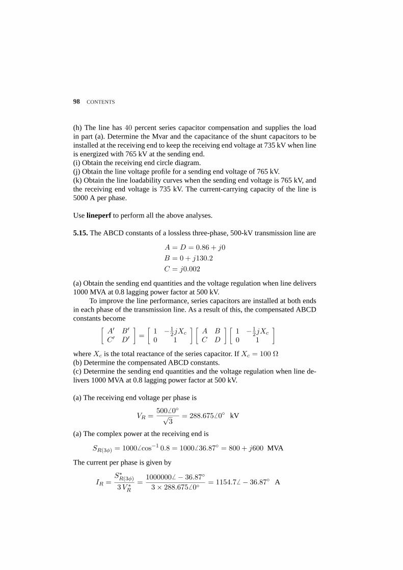
98 CONTENTS
(h) The line has40 percent series capacitor compensation and supplies the loadin part (a). Determine the Mvar and the capacitance of the shunt capacitors to beinstalled at the receiving end to keep the receiving end voltage at 735 kV when lineis energized with 765 kV at the sending end.(i) Obtain the receiving end circle diagram.(j) Obtain the line voltage profile for a sending end voltage of 765 kV.(k) Obtain the line loadability curves when the sending end voltage is 765 kV, andthe receiving end voltage is 735 kV. The current-carrying capacity of the line is5000 A per phase.
Uselineperf to perform all the above analyses.
5.15.The ABCD constants of a lossless three-phase, 500-kV transmission line are
A = D = 0.86 + j0B = 0 + j130.2C = j0.002
(a) Obtain the sending end quantities and the voltage regulation when line delivers1000 MVA at 0.8 lagging power factor at 500 kV.
To improve the line performance, series capacitors are installed at both endsin each phase of the transmission line. As a result of this, the compensated ABCDconstants become
[A′ B′C ′ D′
]=
[1 −1
2jXc
0 1
] [A BC D
] [1 −1
2jXc
0 1
]
whereXc is the total reactance of the series capacitor. IfXc = 100 Ω(b) Determine the compensated ABCD constants.(c) Determine the sending end quantities and the voltage regulation when line de-livers 1000 MVA at 0.8 lagging power factor at 500 kV.
(a) The receiving end voltage per phase is
VR =5006 0√
3= 288.6756 0 kV
(a)The complex power at the receiving end is
SR(3φ) = 10006 cos−1 0.8 = 10006 36.87 = 800 + j600 MVA
The current per phase is given by
IR =S∗R(3φ)
3V ∗R
=10000006 − 36.87
3× 288.6756 0= 1154.76 − 36.87 A
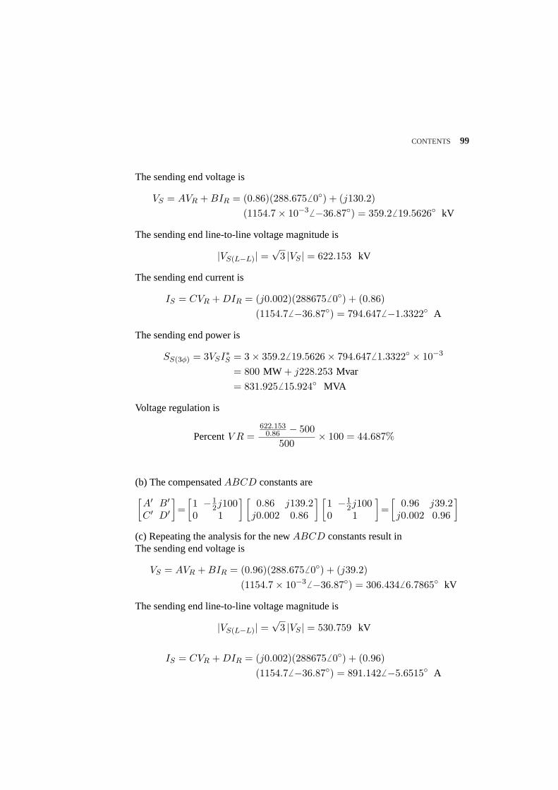
CONTENTS 99
Thesending end voltage is
VS = AVR + BIR = (0.86)(288.6756 0) + (j130.2)(1154.7× 10−3 6 −36.87) = 359.26 19.5626 kV
Thesending end line-to-line voltage magnitude is
|VS(L−L)| =√
3 |VS | = 622.153 kV
The sending end current is
IS = CVR + DIR = (j0.002)(2886756 0) + (0.86)(1154.76 −36.87) = 794.6476 −1.3322 A
Thesending end power is
SS(3φ) = 3VSI∗S = 3× 359.26 19.5626× 794.6476 1.3322 × 10−3
= 800 MW + j228.253 Mvar
= 831.9256 15.924 MVA
Voltage regulation is
PercentV R =622.153
0.86 − 500500
× 100 = 44.687%
(b) The compensatedABCD constants are[A′ B′C ′ D′
]=
[1 −1
2j1000 1
] [0.86 j139.2
j0.002 0.86
] [1 −1
2j1000 1
]=
[0.96 j39.2
j0.002 0.96
]
(c) Repeating the analysis for the newABCD constants result inThe sending end voltage is
VS = AVR + BIR = (0.96)(288.6756 0) + (j39.2)(1154.7× 10−3 6 −36.87) = 306.4346 6.7865 kV
Thesending end line-to-line voltage magnitude is
|VS(L−L)| =√
3 |VS | = 530.759 kV
IS = CVR + DIR = (j0.002)(2886756 0) + (0.96)(1154.76 −36.87) = 891.1426 −5.6515 A

100 CONTENTS
Thesending end power is
SS(3φ) = 3VSI∗S = 3× 306.4346 6.7865× 891.1426 5.6515 × 10−3
= 800 MW + j176.448 Mvar
= 819.2276 12.438 MVA
Voltage regulation is
PercentV R =530.759
0.96 − 500500
× 100 = 10.5748%
We can uselineperf and option 4 to obtain the above solutions.
5.16.A three-phase 420-kV, 60-HZ transmission line is 463 km long and may beassumed lossless. The line is energized with 420 kV at the sending end. When theload at the receiving end is removed, the voltage at the receiving end is 700 kV, andthe per phase sending end current is646.66 90 A.
(a)Find the phase constantβ in radians per Km and the surge impedanceZc in Ω.(b) Ideal reactors are to be installed at the receiving end to keep|VS | = |VR| = 420kV when load is removed. Determine the reactance per phase and the requiredthree-phase Mvar.
(a) The sending end and receiving end voltages per phase are
VS =420√
3= 242.487 kV
VRnl =700√
3= 404.145 kV
With load removedIR = 0, from (5.71) we have
242.487 = (cosβ`)(404.145)
or
β` = 53.13 = 0.927295 Radian
and from (5.72), we have
j646.6 = j1Zc
(sin 53.13)(404.145)103
or
Zc = 500 Ω

CONTENTS 101
(b) ForVS = VR, the required inductor reactance given by (5.100) is
XLsh =sin(53.13)
1− cos(53.13)(500) = 1000 Ω
The three-phase shunt reactor rating is
Q3φ =(KVLrated)2
XLsh=
(420)2
1000= 176.4 Mvar
5.17.A three-phase power of 3600 MW is to be transmitted via four identical 60-Hz transmission lines for a distance of 300 Km. From a preliminary line design, theline phase constant and surge impedance are given byβ = 9.46× 10⁻⁴ radian/KmandZc = 343 Ω, respectively.Based on the practical line loadability criteria determine the suitable nominal volt-age level in kV for each transmission line. AssumeVS = 1.0 pu,VR = 0.9 pu, andthe power angleδ = 36.87.
β` = (9.46× 10⁻⁴)(300)(180π
) = 16.26
The real power per transmission circuit is
P =3600
4= 900 MW
From the practical line loadability given by(5.97), we have
900 =(1.0)(0.9)(SIL)
sin(16.26)sin(36.87)
Thus
SIL = 466.66 MW
From (5.78)
KVL =√
(Zc)(SIL) =√
(343)(466.66) = 400 kV
5.18.Power system studies on an existing system have indicated that 2400 MWare to be transmitted for a distance of 400 Km. The voltage levels being consideredinclude 345 kV, 500 kV, and 765 kV. For a preliminary design based on the practicalline loadability, you may assume the following surge impedances
345 kV ZC = 320 Ω500 kV ZC = 290 Ω765 kV ZC = 265 Ω

102 CONTENTS
Theline wavelength may be assumed to be 5000 Km. The practical line loadabilitymay be based on a load angleδ of 35. Assume|VS | = 1.0 pu and|VR| = 0.9pu. Determine the number of three-phase transmission circuits required for eachvoltage level. Each transmission tower may have up to two circuits. To limit thecorona loss, all 500-kV lines must have at least two conductors per phase, and all765-kV lines must have at least four conductors per phase. The bundle spacing is45 cm. The conductor size should be such that the line would be capable of carry-ing current corresponding to at least 5000 MVA. Useacsrcommand inMATLABtofind a suitable conductor size. Following are the minimum recommended spacingsbetween adjacent phase conductors at various voltage levels.
Voltage level, kV Spacing meter345 7.0500 9.0765 12.5
(a) Select a suitable voltage level, and conductor size, and tower structure. Uselineperf program and option 1 to obtain the voltage regulation and transmissionefficiency based on a receiving end power of 3000 MVA at 0.8 power factor lag-ging at the selected rated voltage. Modify your design and select a conductor sizefor a line efficiency of at least94 percent for the above specified load.(b) Obtain the line performance including options 4–8 of thelineperf program foryour final selection. Summarize the line characteristics and the required line com-pensation.
For each voltage levelSIL is computed from (5.78). From the practical line load-ability equation given by (5.97), the real power per circuit is computed, and numberof circuits is established and tabulated in the following table.
Voltage Surge SIL Power/ No.ofKV Imp.,Ω MW circuit circuit
345 320 371.95 398.56 2400398.56 = 6
500 290 862.07 923.74 2400923.74 = 3
765 265 2208.39 2366.39 24002366.39 = 1
For the 345 kV level we require six three-phase transmission circuit, and for the500 kV line we need three circuits. Considering the cost of the transmission towers,right of ways and associated equipment, it can be concluded that one circuit at 765kV is the most economical and practical choice.
Using the 765 kV for transmission line voltage, the per phase current corre-

CONTENTS 103
spondingto 5000 MVA maximum is
I =5000× 103
√3 765
= 3773.5 A
Since we have four conductor per phase, then current per conductor is
Icond =3773.5
4= 943.38 A
From theacsr file we select the CRANE conductor with a current-carrying capac-ity of 950 A. Typing acsr at theMATLABprompt and selecting ’crane’, result in
Enter ACSR code name within single quotes -> ’crane’Al Area Strand Diameter GMR Resistance Ohm/km Ampacitycmil Al/St cm cm 60Hz 25C 60Hz 50C Ampere874500 54/7 2.9108 1.1765 0.06712 0.07632 950
Using lineperf result in
TRANSMISSION LINE MODELType of parameters for input Select
Parameters per unit lengthr(ohm), g(seimens) L(mH) & C (micro F) 1
Complex z and y per unit lengthr+j*x (ohm/length), g+j*b (seimens/length) 2
Nominal pi or Eq. pi model 3
A, B, C, D constants 4
Conductor configuration and dimension 5
To quit 0
Select number of menu --> 5Enter spacing unit within quotes ’m’ or ’ft’-> ’m’Enter row vector [D12, D23, D13] = [12.5 12.5 25]Cond. size, bundle spacing unit: Enter ’cm’ or ’in’-> ’cm’Conductor diameter in cm = 2.9108Geometric Mean Radius in cm = 1.1765No. of bundled cond. (enter 1 for single cond.) = 4Bundle spacing in cm = 45
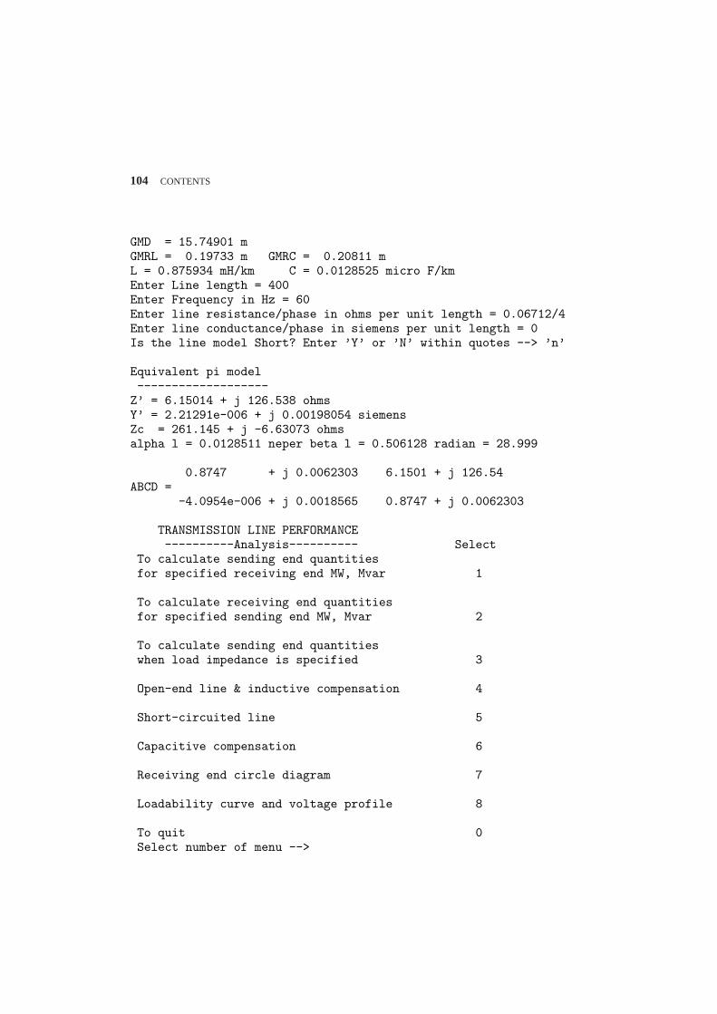
104 CONTENTS
GMD = 15.74901 mGMRL = 0.19733 m GMRC = 0.20811 mL = 0.875934 mH/km C = 0.0128525 micro F/kmEnter Line length = 400Enter Frequency in Hz = 60Enter line resistance/phase in ohms per unit length = 0.06712/4Enter line conductance/phase in siemens per unit length = 0Is the line model Short? Enter ’Y’ or ’N’ within quotes --> ’n’
Equivalent pi model-------------------
Z’ = 6.15014 + j 126.538 ohmsY’ = 2.21291e-006 + j 0.00198054 siemensZc = 261.145 + j -6.63073 ohmsalpha l = 0.0128511 neper beta l = 0.506128 radian = 28.999
0.8747 + j 0.0062303 6.1501 + j 126.54ABCD =
-4.0954e-006 + j 0.0018565 0.8747 + j 0.0062303
TRANSMISSION LINE PERFORMANCE----------Analysis---------- Select
To calculate sending end quantitiesfor specified receiving end MW, Mvar 1
To calculate receiving end quantitiesfor specified sending end MW, Mvar 2
To calculate sending end quantitieswhen load impedance is specified 3
Open-end line & inductive compensation 4
Short-circuited line 5
Capacitive compensation 6
Receiving end circle diagram 7
Loadability curve and voltage profile 8
To quit 0Select number of menu -->

CONTENTS 105
Selectingoptions 1 through 8 result in
Line performance for specified receiving end quantities-------------------------------------------------------Vr = 765 kV (L-L) at 0Pr = 2400 MW Qr = 1800 MvarIr = 2264.12 A at -36.8699 PFr = 0.8 laggingVs = 1059.49 kV (L-L) at 21.4402Is = 1630.56 A at -12.6476 PFs = 0.82818 laggingPs = 2478.108 MW Qs = 1677.037 MvarPL = 78.108 MW QL = -122.963 MvarPercent Voltage Regulation = 58.3312Transmission line efficiency = 96.8481
Open line and shunt reactor compensation----------------------------------------Vs = 765 kV (L-L) at 0Vr = 874.563 kV (L-L) at -0.00712268Is = 937.387 A at 89.7183 PFs = 0.00491663 leading
Desired no load receiving end voltage = 765 kVShunt reactor reactance = 1009.82 ohmShunt reactor rating = 579.531 MvarHit return to continue
Line short-circuited at the receiving end-----------------------------------------Vs = 765 kV (L-L) at 0Ir = 3486.33 A at -87.2174Is = 3049.57 A at -86.8093
Shunt capacitive compensation-----------------------------Vs = 765 kV (L-L) at 31.8442Vr = 765 kV (L-L) at 0Pload = 2400 MW Qload = 1800 MvarLoad current = 2264.12 A at -36.8699 PFl = 0.8 laggingRequired shunt capcitor:287.826ohm,9.21593microF,2033.26 MvarShunt capacitor current = 1534.51 A at 90Pr = 2400.000 MW Qr = -233.261 MvarIr = 1819.83 A at 5.55126 PFr = 0.99531 leadingIs = 1863.22 A at 31.9226 PFs = 0.999999 leadingPs = 2468.802 MW Qs = -3.378 MvarPL = 68.802 MW QL = 229.882 MvarPercent Voltage Regulation = 14.322

106 CONTENTS
Transmission line efficiency = 97.2131
Series capacitor compensation-----------------------------Vr = 765 kV (L-L) at 0Pr = 2400 MW Qr = 1800 MvarRequired series capacitor:50.6151ohm,52.4069microF, 209.09MvarSubsynchronous resonant frequency = 37.9473 HzIr = 2264.12 A at -36.8699 PFr = 0.8 laggingVs = 933.799 kV (L-L) at 14.1603Is = 1729.43 A at -13.485 PFs = 0.885837 laggingPs = 2477.831 MW Qs = 1297.875 MvarPL = 77.831 MW QL = -502.125 MvarPercent Voltage Regulation = 31.9848Transmission line efficiency = 96.8589
Series and shunt capacitor compensation---------------------------------------Vs = 765 kV (L-L) at 18.5228Vr = 765 kV (L-L) at 0Pload = 2400 MW Qload = 1800 MvarLoad current = 2264.12 A at -36.8699 PFl = 0.8 laggingRequired shunt capcitor: 322.574ohm, 8.22319microF,1814.24MvarShunt capacitor current = 1369.22 A at 90Required series capacitor:50.6151ohm,52.4069microF,176.311MvarSubsynchronous resonant frequency = 37.9473 HzPr = 2400 MW Qr = -14.2373 MvarIr = 1811.33 A at 0.339886 PFr = 0.999982 leadingIs = 1882.74 A at 27.2821 PFs = 0.988337 leadingPs = 2465.565 MW Qs = -379.900 MvarPL = 65.565 MW QL = -365.662 MvarPercent Voltage Regulation = 8.12641Transmission line efficiency = 97.3408
To transmit 2400 MW for a distance of 400 Km, we select a horizontal tower at 765kV with four ACSR crane conductor per phase. The recommended compensatorsare:
• A three-phase shunt reactor for the open-ended line with a maximum ratingof 580 Mvar at 765 kV.
• A three-phase shunt capacitor with a maximum rating of 1815 Mvar at 765kV.
• A three-phase series capacitor with a maximum rating of 176 Mvar, 765 kV.


![Power System Analysis by Hadi Saadat Electrical Engineering[1]](https://img.pdfslide.us/doc/110x75/55cf94bd550346f57ba41826/power-system-analysis-by-hadi-saadat-electrical-engineering1.jpg)