SOLUTION QUANTITATIVE TOOLS IN BUSINESS NOV … · · 2014-05-22Y = 44.5 + 10.5x (b) ... The trendline 48.64 + 0.77x used to do estimates: x (quarters) y (Revenue) Estimated

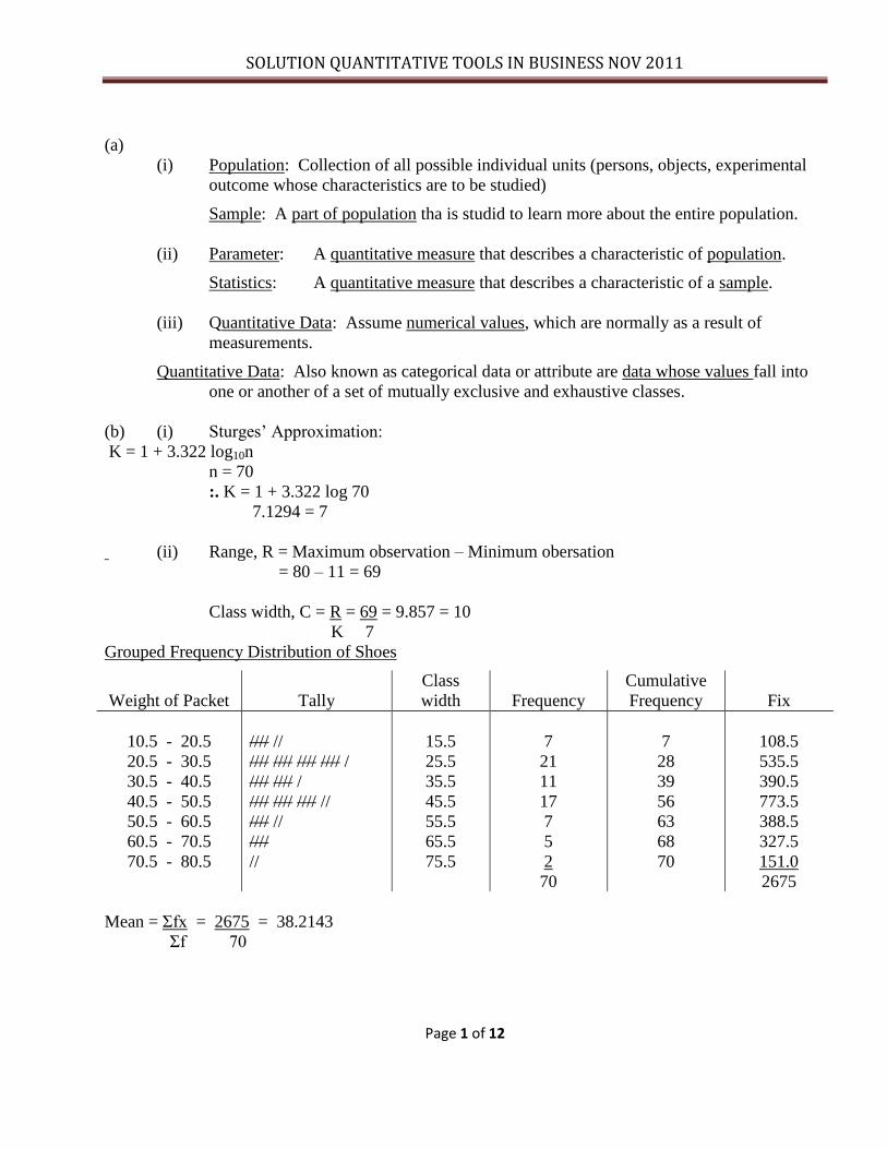
SOLUTION QUANTITATIVE TOOLS IN BUSINESS NOV 2011

Page 1 of 12

(a)

(i) Population: Collection of all possible individual units (persons, objects, experimental

outcome whose characteristics are to be studied)

Sample: A part of population tha is studid to learn more about the entire population.

(ii) Parameter: A quantitative measure that describes a characteristic of population.

Statistics: A quantitative measure that describes a characteristic of a sample.

(iii) Quantitative Data: Assume numerical values, which are normally as a result of

measurements.

Quantitative Data: Also known as categorical data or attribute are data whose values fall into

one or another of a set of mutually exclusive and exhaustive classes.

(b) (i) Sturges’ Approximation:

K = 1 + 3.322 log10n

n = 70

:. K = 1 + 3.322 log 70

7.1294 = 7

(ii) Range, R = Maximum observation – Minimum obersation

= 80 – 11 = 69

Class width, C = R = 69 = 9.857 = 10

K 7

Grouped Frequency Distribution of Shoes

Weight of Packet

Tally

Class

width

Frequency

Cumulative

Frequency

Fix

10.5 - 20.5

20.5 - 30.5

30.5 - 40.5

40.5 - 50.5

50.5 - 60.5

60.5 - 70.5

70.5 - 80.5

//// //

//// //// //// //// /

//// //// /

//// //// //// //

//// //

////

//

15.5

25.5

35.5

45.5

55.5

65.5

75.5

7

21

11

17

7

5

2

70

7

28

39

56

63

68

70

108.5

535.5

390.5

773.5

388.5

327.5

151.0

2675

Mean = Σfx = 2675 = 38.2143

Σf 70


Page 2 of 12

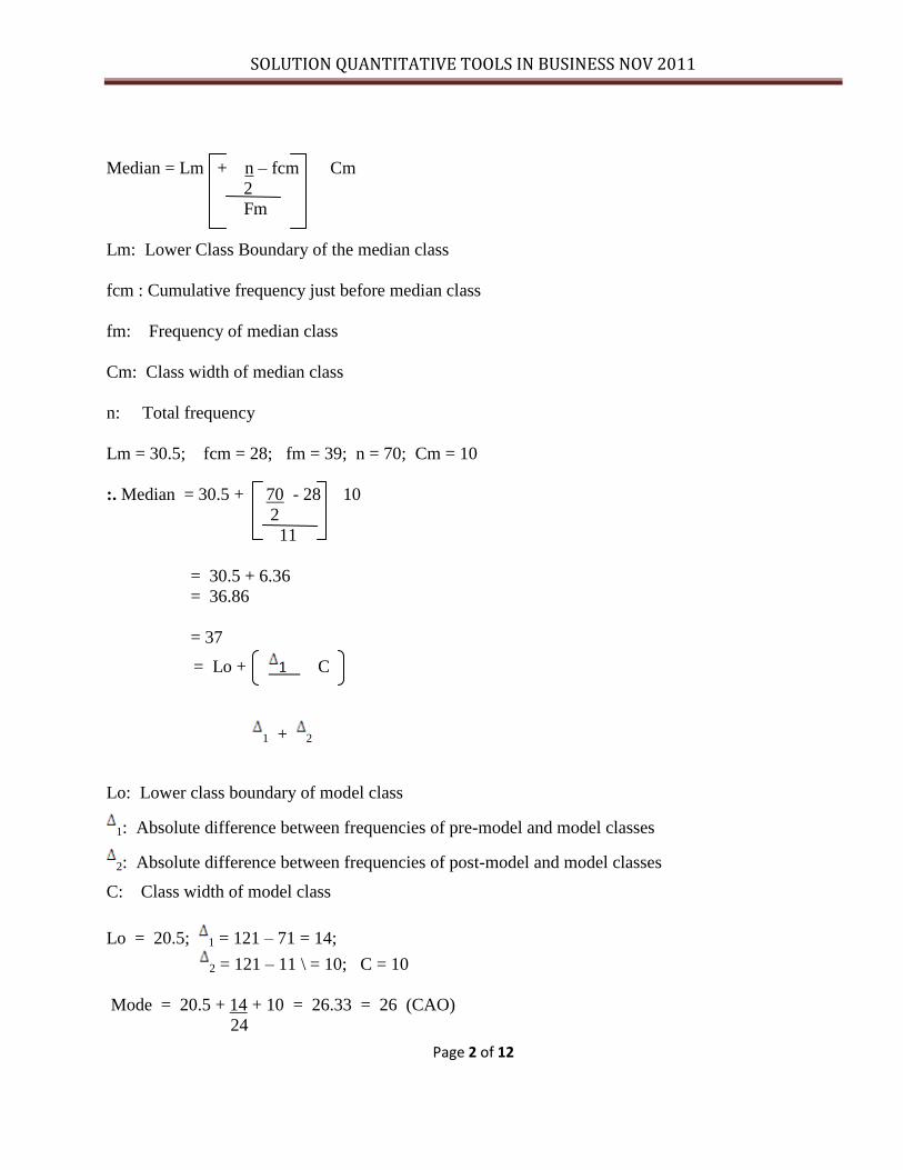
Median = Lm + n – fcm Cm

2

Fm

Lm: Lower Class Boundary of the median class

fcm : Cumulative frequency just before median class

fm: Frequency of median class

Cm: Class width of median class

n: Total frequency

Lm = 30.5; fcm = 28; fm = 39; n = 70; Cm = 10

:. Median = 30.5 + 70 - 28 10

2

11

= 30.5 + 6.36

= 36.86

= 37

= Lo + 1 C

1 + 2

Lo: Lower class boundary of model class

1: Absolute difference between frequencies of pre-model and model classes

2: Absolute difference between frequencies of post-model and model classes

C: Class width of model class

Lo = 20.5; 1 = 121 – 71 = 14;

2 = 121 – 11 \ = 10; C = 10

Mode = 20.5 + 14 + 10 = 26.33 = 26 (CAO)

24


Page 3 of 12

SOLUTION 2

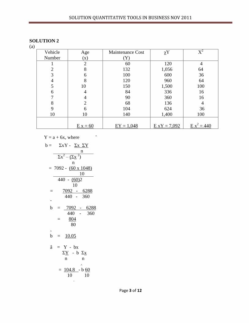
(a)

Vehicle

Number

Age

(x)

Maintenance Cost

(Y)

χY Χ2

1

2

3

4

5

6

7

8

9

10

2

8

6

8

10

4

4

2

6

10

60

132

100

120

150

84

90

68

104

140

120

1,056

600

960

1,500

336

360

136

624

1,400

4

64

36

64

100

16

16

4

36

100

E x = 60

EY = 1,048

E xY = 7,092

E x2 = 440

Y = a + 6x, where ˆ

b = ΣxY - Σx ΣY

n

Σx2 – (Σx

2)

n

= 7092 - (60 x 1048)

10

440 - (60)2

10

= 7092 - 6288

440 - 360

ˆ

b = 7092 - 6288

440 - 360

= 804

80

^

b = 10.05

â = Y - bx

ΣY - b Σx

n n

^

= 104.8 - b 60

10 10

ˆ


Page 4 of 12

â = 104.8 – b, where b = 10.05

â = 104.8 – 10.05x

â = 104.8 – 60.3

â = 44.5

:. Y = 44.5 + 10.5x

(b) Maintenance Cost Table

Years

(x)

_ Module

Y = 44.5 + 10.05 x

Maintenance Cost

GHS

1

2

3

4

5

6

7

8

9

10

44.5 + 10.05 (1)

44.5 + 10.05 (2)

44.5 + 10.05 (3)

44.5 + 10.05 (4)

44.5 + 10.05 (5)

44.5 + 10.05 (6)

44.5 + 10.05 (7)

44.5 + 10.05 (8)

44.5 + 10.05 (9)

44.5 + 10.05 (10)

54.55

64.60

74.65

84.70

94.75

104.80

114.85

124.90

134.95

145.00

(c) Estinmate cost of maintaining a 12 year old vehicle

_

Y = 44.5 + 10.05x, where x = 12

_

Y = 44.5 + 10.05 (12)

Y = 165.10

_ _ ^

When there is a change in x, Y change by b, where â is constant.

SOLUTION 3

(a)

(i) NPV ÷ is the present value of cash flows minus the present value of cash outflows

n n

NPV= Σ cash inflow at time t Σ Cash outflow at time t

t = o (l + i) t (l + i)

t

t = o


Page 5 of 12

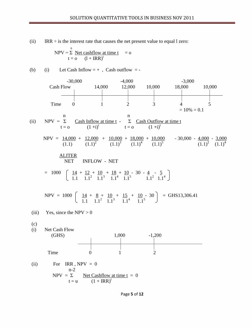
(ii) IRR ÷ is the interest rate that causes the net present value to equal l zero:

n

NPV = Σ Net cashflow at time t = o

t = o (l + IRR)t

(b) (i) Let Cash Inflow = + , Cash outflow = -

-30,000 -4,000 -3,000

Cash Flow 14,000 12,000 10,000 18,000 10,000

Time 0 1 2 3 4 5

= 10% = 0.1

n n

(ii) NPV = Σ Cash Inflow at time t - Σ Cash Outflow at time t

t = o (1 +i)t t = o (1 +i)

t

NPV = 14,000 + 12,000 + 10,000 + 18,000 + 10,000 - 30,000 - 4,000 - 3,000

(1.1) (1.1)2 (1.1)

3 (1.1)

4 (1.1)

5 (1.1)

2 (1.1)

4

ALITER

NET INFLOW - NET

= 1000 14 + 12 + 10 + 18 + 10 - 30 - 4 - 5

1.1 1.12 1.1

3 1.1

4 1.1

5 1.1

2 1.1

4

NPV = 1000 14 + 8 + 10 + 15 + 10 - 30 = GHS13,306.41

1.1 1.12 1.1

3 1.1

4 1.1

5

(iii) Yes, since the NPV > 0

(c)

(i) Net Cash Flow

(GHS) 1,000 -1,200

Time 0 1 2

(ii) For IRR , NPV = 0

n-2

NPV = Σ Net Cashflow at time t = 0

t = u (1 + IRR)t


Page 6 of 12

1000 - 1200 = 0

(1 + IRR) (1 + IRR)2

1000 (1 + IRR) - 1200 = 0

(1 + IRR) = 1200 = 1.2

1000

= IRR = 0.2 or 20%

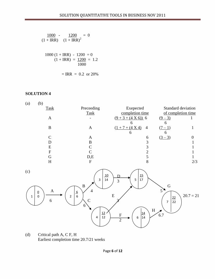
SOLUTION 4

(a) (b)

Task Preceeding

Task

Exepected

completion time

Standard deviation

of completion time

A

B

C

D

E

F

G

H

-

A

A

B

C

C

D,E

F

(9 + 3 + (4 X 6)) 6

6

(1 + 7 + (4 X 4) 4

6

6

3

3

2

5

8

(9 – 3) 1

6

(7 – 1) 1

6

(3 – 3) 0

1

1

1

1

2/3

(c)

D

3

B G

A 4 5

E 20.7 = 21

6 C 3

6

H

F 6.7

2

(d) Critical path A, C F, H

Earliest completion time 20.7/21 weeks

10 3 14

15 5 17

0 1 0

6 2 6

12 4 12

14 6 14

22 7 22


Page 7 of 12

(e) Variance of critical path = (12

+ 12 + 1

2 + 2/3

2)

= 3 4/9

Standard deviation = 1.857

(f) Project completion time = 21 weeks

Standard deviation = 1.857 weeks

Prob (less then 20 weeks) : 20 – 21

Z = 1.857

Z = 0.5385

From normal distribution tables P(Z < -0.5385) = 0.5 – 0.2054

= 0.2946

SOLUTION 5

(a) Basic laws of Probability:

- Multiplicative Law states that:

If A and B are independent events then P(A B) = P(A)P(B)

(i) If A and B are dependent events then P(A B) = P(A)P(B/A) = P(B)P(A/B)

- Additive law states that:

(i) If A and B are events then:

P(A B) = P(A) + P(B) – P(A B)

If A and B are mutually exclusive events then P(A B) = P(A) + P(B)

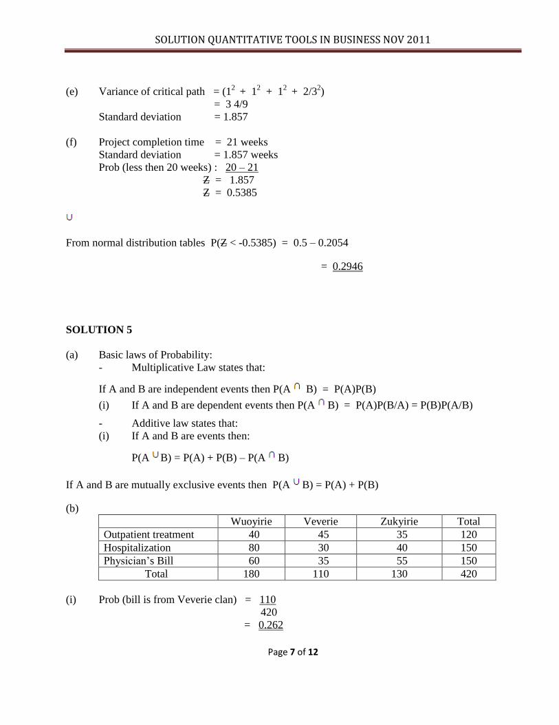
(b)

Wuoyirie Veverie Zukyirie Total

Outpatient treatment 40 45 35 120

Hospitalization 80 30 40 150

Physician’s Bill 60 35 55 150

Total 180 110 130 420

(i) Prob (bill is from Veverie clan) = 110

420

= 0.262


Page 8 of 12

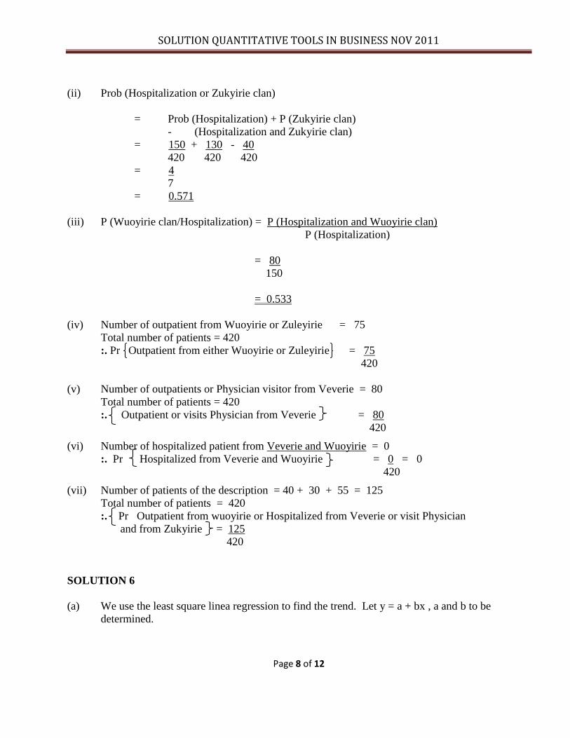
(ii) Prob (Hospitalization or Zukyirie clan)

= Prob (Hospitalization) + P (Zukyirie clan)

- (Hospitalization and Zukyirie clan)

= 150 + 130 - 40

420 420 420

= 4

7

= 0.571

(iii) P (Wuoyirie clan/Hospitalization) = P (Hospitalization and Wuoyirie clan)

P (Hospitalization)

= 80

150

= 0.533

(iv) Number of outpatient from Wuoyirie or Zuleyirie = 75

Total number of patients = 420

:. Pr Outpatient from either Wuoyirie or Zuleyirie = 75

420

(v) Number of outpatients or Physician visitor from Veverie = 80


:. Outpatient or visits Physician from Veverie = 80

420

(vi) Number of hospitalized patient from Veverie and Wuoyirie = 0

:. Pr Hospitalized from Veverie and Wuoyirie = 0 = 0

420

(vii) Number of patients of the description = 40 + 30 + 55 = 125


:. Pr Outpatient from wuoyirie or Hospitalized from Veverie or visit Physician

and from Zukyirie = 125

420

SOLUTION 6

(a) We use the least square linea regression to find the trend. Let y = a + bx , a and b to be

determined.


Page 9 of 12

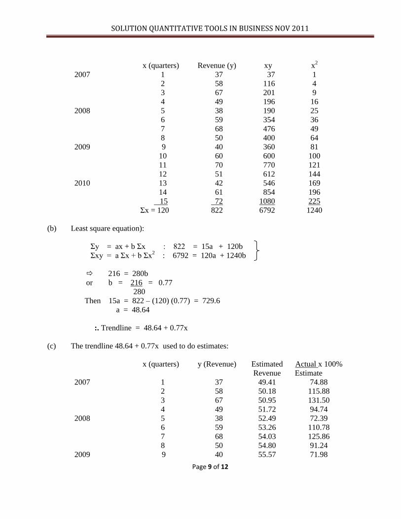
x (quarters) Revenue (y) xy x2

2007

2008

2009

2010

1

2

3

4

5

6

7

8

9

10

11

12

13

14

15

Σx = 120

37

58

67

49

38

59

68

50

40

60

70

51

42

61

72

822

37

116

201

196

190

354

476

400

360

600

770

612

546

854

1080

6792

1

4

9

16

25

36

49

64

81

100

121

144

169

196

225

1240

(b) Least square equation):

Σy = ax + b Σx : 822 = 15a + 120b

Σxy = a Σx + b Σx2 : 6792 = 120a + 1240b

216 = 280b

or b = 216 = 0.77

280

Then 15a = 822 – (120) (0.77) = 729.6

a = 48.64

:. Trendline = 48.64 + 0.77x

(c) The trendline 48.64 + 0.77x used to do estimates:

x (quarters) y (Revenue) Estimated

Revenue

Actual x 100%

Estimate

2007

2008

2009

1

2

3

4

5

6

7

8

9

37

58

67

49

38

59

68

50

40

49.41

50.18

50.95

51.72

52.49

53.26

54.03

54.80

55.57

74.88

115.88

131.50

94.74

72.39

110.78

125.86

91.24

71.98


Page 10 of 12

2010

10

11

12

13

14

15

60

70

51

42

61

72

56.34

57.11

57.88

58.65

59.42

60.19

106.50

122.57

88.11

71.61

102.66

119.62

2007: 1st Quarter Estimate = 48.64 + 0.77 (1) = 49.41

2nd

Quarter Estimate = 48.64 + 0.77 (2) = 50.18 etc.

(d) Averaging the % variation for the quarters

Q1 Q2 Q3 Q4

75

72

72

72

291

116

111

107

103

437

132

126

123

120

501

95

91

88

274

291/42 437/4

2 501/4

2 274/3

2

Average Seasonal

Variations 73% 109% 125% 91%

(e) Seasonally adjusted forecast = Trend Estimate x Seasonal Variations %

x (quarters) y (Revenue) Seasonally

adjusted

forecast

2007

2008

2009

2010

1

2

3

4

5

6

7

8

9

10

11

12

13

14

15

37

58

67

49

38

59

68

50

40

60

70

51

42

61

72

36.07

54.50

63.69

47.07

38.32

58.05

67.54

49.87

40.57

61.41

71.39

52.67

42.81

64.77

75.24


Page 11 of 12

(f) From the trendline, the 4th

quarter of 2010 is obtained as follows:

Basic trnd = 48.64 + 0.77 (16)

= 60.96

Seasonal adjustment for 4th

Quarter = 91%

:. Adjusted Forecast = 60.96 x 91%

= 55.47

SOLUTION 7

(a) Reasons include:

1. Protection against delayed supply

2. Protection against fluactuating demand

3. Protection against price changes (inflation)

4. Savings or ordering cost

5. Benefits of large quantities discount

(b) Assumptions are:

1. The demand for the item is constant over time.

2. Within the range of quantities to be ordered, the per unit holding cost and ordering cost

are independent of the quantity ordered.

3. The replenishment arrives exactly when the inventory level reaches zero.

(c) (i) Demand (D) = GHS500.00

Ordering cost (K) = GHS8.00

Holding cost (H) = 0.2 (20%)

____ _________ ______

EOQ = √2DK = √ 2 x 8 x 500 = √ 40,000 = GHS200

H 0.2

(ii) Annual demand GHS500.00

EOQ = GHS200.00

:. Number of times orders are placed in a year = D/EOQ = 500 = 2.5 times

200

Approximately 3 times

(ii) Total annual ordering cost = Number of orders in a year x ordering cost

= 2.5 x 8 = GHS20.00


Page 12 of 12

(iii) Total annual holding cost = HD

2

= 0.2 x 200 = GHS20.00

2

(iv) If D quadruples from 500 to 2,000

the EOQ = __________ ______

√2 x 8 x 2000 = √160000

0.2

= GHS400.00

EOQ douples from GHS200 to GHS400 ie GHS200

Documents

SOLUTION QUANTITATIVE TOOLS IN BUSINESS NOV … · · 2014-05-22Y = 44.5 + 10.5x (b) ... The trendline 48.64 + 0.77x used to do estimates: x (quarters) y (Revenue) Estimated