Embed Size (px)
Citation preview

1
CHAPTER 15
Solution of Transient and DynamicProblems Using the Finite Element Method
15.0. General Remarks
In the boundary value problems analyzed previously, steady state conditions were
assumed; i.e., the solution sought was taken to be independent of time. In a large number of
practical problems the conditions are, however, time dependent (often termed transient,
dynamic or unsteady). As such, their solution requires consideration of the time domain.
The differential equation governing time dependent problems can be written in the
following general form
L(φ ) − f − a∂φ∂ t
− b∂ 2φ∂ t2 = 0 in Ω (15.1)
In equation (15.1) φ denotes the primary dependent variable; the independent variables
are the spatial coordinates (x1, x2 ,x3) and the time t. In equation (15.1) L represents a linear
operator involving differentiation with respect to the spatial coordinates only. In the mostgeneral case, the quantities f, a and b are prescribed functions of (x1, x2 ,x3) , t and, in non-
linear cases, of φ . Equation (15.1) is supplemented by suitable boundary-conditions and,
unlike the problems previously considered, initial conditions.
Before proceeding to develop finite element equations for use in solving time dependent
problems, it is instructive to consider some specific examples of physical problems governed
by equation (15.1). Further examples of such problems are found in standard texts on partial
differential equations e.g., [1]; the solution of such problems using the finite element method is
discussed in, for example [2-5].

2 The Finite Element Method : Intermediate Topics
Example 15.1 : Three-Dimensional Transient Heat Conduction 1
In a thermally isotropic material the variation of temperature T is governed by thefollowing (parabolic) partial differential equation :
∂∂x1
k∂T
∂x1
+
∂∂x2
k∂T
∂x2
+
∂∂x3
k∂T
∂x3
+ S − ρcv
∂T
∂t= 0 (1)
implying that, with respect to equation (15.1),
φ = T (2)
L =∂
∂x1
k∂
∂x1
+
∂∂x2
k∂
∂x2
+
∂∂x3
k∂
∂x3
(3)
f =− S (4)
a = ρcv (5)
b = 0 (6)
The boundary conditions are
Dirichlet :
T = T on ΓD ∀ t > 0 (7)
Neumann :
−k∂T
∂n= q n on ΓN ∀ t > 0 (8)
where n denotes the unit outward normal along Γ N . The initial condition is
T = T 0 at t = 0 ∀ (x1 , x2 , x3) ∈Ω (9)
In the above equations barred values represent known (specified) quantities, and
k = the coefficient of thermal conductivity (typical units : J/s - m - oK );S = a source (or sink) term (typical units : J/s - m3 );ρ = the mass density of the material (typical units : kg / m3 );cv = the specific heat at constant volume (typical units : J/kg - oK );qn = the heat flux per unit area flowing at the boundary whose outward unit normal
vector is n♦
1 Further details regarding heat conduction are given in the appendix titled “Further details regarding heat
conduction are given in the appendix titled “Some Notes on Heat Flow”( http://www.ce.udel.edu/faculty/kaliakin/appendix_heat.pdf ).

Chapter 15 : Solution of Transient and Dynamic Problems Using the FEM 3
Example 15.2 : One-Dimensional Diffusion-Convection Equation
Consider the case of a pollutant being carried along in a stream moving with a velocity v.The concentration u(x,t) of the pollutant changes as a function of both the spatial variablex (positive x is measured downstream) and time t . The rate of change of the concentrationis described by the so-called “diffusion-convection equation” (a parabolic PDE) :
∂u
∂ t− γ 2 ∂ 2u
∂x2 + η∂u
∂x= 0 in Ω (1)
where η represents the diffusion coefficient. Comparing equation (1) with equation(15.1), it is evident that the former is obtained from the latter by setting
φ = u (2)
L =− γ 2 ∂ 2
∂x2 + η∂∂x
(3)
f = 0 (4)
a = −1 (5)
b = 0 (6)
The boundary conditions are typically
u = u on Γ D ∀ t > 0 (7)
The initial condition is
u = u 0 at t = 0 ∀ x ∈Ω (8)
In equation (1) the term γ 2u,xx represents the diffusion contribution; i.e., that attributed tothe mixing of the substance through the stream’s fluid. The term ηu, x represents theconvection component; i.e., that attributed to the movement of the substance by means ofthe medium. Whether the pollutant primarily diffuses or convects depends upon the relativemagnitude of the two parameters γ and η .
♦

4 The Finite Element Method : Intermediate Topics
Example 15.3 : One- and Two-Dimensional Wave Equation
By setting
L = τ∂ 2
∂x2 − γ (1)
f =− f (x,t) (2)
a = µ (3)and
b = ρ (4)
Equation (15.1) is transformed into the most general form of the one-dimensional waveequation (a hyperbolic PDE)
τ∂ 2φ∂x2 − γφ + f (x,t) − µ
∂φ∂ t
− ρ∂ 2φ∂t2 = 0 (5)
If φ = u , where u represents the transverse vibration of a string, then equation (5)becomes the so-called “telephone equation” [1]. Now ρ represents the mass per unit lengthof the string, τ denotes the force in the string, τu, xx represents the net force due to thetension of the string, µu,t represents the frictional (damping) force acting against the string(e.g., the string is vibrating in a medium that offers resistance to the string’s velocity); µwill thus have the units of (FL-2 t). The quantity γu represents a restoring force; i.e., aforce that is directed opposite to the displacement of the string; γ will thus have units of(FL-2). Finally, f (x,t) represents an external force per unit length applied at any pointalong the string at any time t. For example, f (x,t) could be a gravitational force, animpulse loading, etc.
If f (x,t) = 0, equation (5) reduces to the so-called “transmission line” equation
τ∂ 2u
∂x 2 − γu − µ∂u
∂ t− ρ
∂ 2u
∂ t2 = 0 (6)
In the absence of restoring force, equation (6) further reduces to a damped wave equationor, for the specific case considered herein, to the equation for a vibrating string withfriction; i.e.,
τ∂ 2u
∂x 2 − µ∂u
∂ t− ρ
∂ 2u
∂ t2 = 0 (7)
Finally, if friction is neglected, equation (7) reduces to the one-dimensional wave equationor, for the specific case considered herein, to the equation for a vibrating string withoutfriction; i.e.,
∂ 2u
∂ t2 = c2 ∂ 2u
∂x2 (8)

Chapter 15 : Solution of Transient and Dynamic Problems Using the FEM 5
where c = τ / ρ has units of velocity (Lt -1). Although presented in the context of avibrating string, the one-dimensional wave equation governs a wide range of physicalphenomena. For example:
• sound (longitudinal) waves• electromagnetic waves of light and electricity• longitudinal, transverse and torsional vibrations in solids• water (transverse) waves• probability waves in quantum mechanics
Extending the simple wave equation to two dimensions yields the governing differentialequation for a vibrating membrane (e.g., a drumhead); i.e.,
τ∂ 2w
∂x 2 +∂ 2w
∂y2
− f (x, y,t) − ρ
∂ 2 w
∂ t2 = 0 (9)
or more compactlyτ∇2w − f (x, y,t) − ρw,tt = 0 (10)
In light of equation (15.1), it follows that
φ = w (11)
L = τ∂ 2
∂x2 +∂ 2
∂y2
(12)
f = f (x, y,t) (13)
a = 0 (14)
b = ρ (15)where
w = the transverse displacement of the membrane (units : L);f = an applied force per unit area (units : FL-2);ρ = the mass per unit area (units : ML-2); and,τ = the tensile force, per unit length, present on the membrane (units : FL-1).
If f = 0 equation (9) reduces to the classical two-dimensional wave equation c2∇2w = w,tt .
♦
Some approaches to solving time dependent boundary value problems are now
discussed.

6 The Finite Element Method : Intermediate Topics
15.1. Representation of the Time Dimension
In the solution of transient and dynamic problems using the finite element method, two
general approaches exist for representing the time dimension. These are commonly referred to
as “partial” or “semi-discretization” and the “discrete approximation” in time. Although the first
approach is more commonly used, the latter has likewise found application in the literature [4].
The basis behind both approaches is now briefly discussed.
15.1.1. Partial (semi) Discretization
The approximating function for a given element is given by
ˆ φ (x1 , x2, x3,t) = ˆ φ ( p)(t) Npp =1
P
∑ (x1, x2 , x3) (15.2)
where the Np represents a suitable set of element interpolation functions, and ˆ φ (p ) denote the
nodal unknown values of the primary dependent variable. The names “partial- ” or “semi-
discretization” come from the fact that in equation (15.2) only the spatial domain is discretized;
no restrictions regarding the variation of the time domain are imposed.
In light of equation (15.2), it follows that the time derivatives of ˆ φ are given by
∂ ˆ φ ∂t
=∂ ˆ φ ( p)
∂tNp
p =1
P
∑ (15.3)
and∂2 ˆ φ ∂t 2 =
∂ 2 ˆ φ ( p )
∂t2 Npp =1
P
∑ (15.4)
To gain further insight into the approximate solution of equation (15.1) using partial
discretization, write the weighted residual form of this equation; viz. ,
wi L( ˆ φ ) − f − a∂ ˆ φ ∂t
− b∂2 ˆ φ ∂t2
Ω (e )∫ dΩ = 0 (15.5)
where wi denotes a set of appropriate weighting functions, and i =1,2,L ,P . Note that
associated with the operator L are spatial derivatives of ˆ φ ; in an effort to reduce the order of
differentiation of these derivatives, Green’s theorem (integration by parts) is typically applied
to this term. Substituting equations (15.2) to (15.4) into equation (15.5) gives

Chapter 15 : Solution of Transient and Dynamic Problems Using the FEM 7
wib∂2 ˆ φ ( p )
∂t2 Npp =1
P
∑
Ω (e )∫ dΩ+ wia
∂ ˆ φ ( p)
∂tNp
p =1
P
∑
Ω (e )∫ dΩ− wiL
ˆ φ ( p ) Npp=1
P
∑
Ω(e )∫ dΩ
= wi fΩ (e )∫ dΩ (15.6)
Written in matrix form, equation (15.6) becomes
M ( e )[ ] ˆ ˙ φ n + C ( e)[ ] ˆ ˙ φ n + K (e)[ ] ˆ φ n = f ( e) (15.7)
where
mip( e) = wibNp( )
Ω( e)∫ dΩ (15.8)
cip( e) = wiaNp( )
Ω (e )∫ dΩ (15.9)
kip(e ) = − wiL(Np)( )
Ω (e )∫ dΩ (15.10)
fi(e) = wi f
Ω (e )∫ dΩ (15.11)
ˆ ˙ φ n ≡∂ 2 ˆ φ n∂t2
(15.12)
and
ˆ ˙ φ n ≡∂ ˆ φ n∂t
(15.13)
Recall that determination of K ( e )[ ] typically involves the application of Green’s theorem
(integration by parts) to the terms associated with the operator L . Consequently, equation
(15.10) describes positive entries, and a related boundary integral term is likewise generated.Finally, for a Galerkin form of the weighted residual statement, wi ≡ Ni . In such a case,
it is evident from equations (15.8) and (15.9) that M ( e )[ ] and C( e)[ ] are symmetric.
Furthermore, M ( e )[ ] is positive definite matrices, and C( e)[ ] and K ( e )[ ] are positive semi-
definite.

8 The Finite Element Method : Intermediate Topics
15.1.2. Discrete Approximation in Time
In a given time interval ∆tm such as that shown in Figure 15.1.
time
t∆
t m+1tm
m
Figure 15.1. Typical Solution Time Step
With ( m ) ˆ φ ( n) known, write
ˆ φ (τ)=( m ) ˆ φ ( n) +τ
∆tm
( m +1) ˆ φ (n ) −( m ) ˆ φ ( n)( ) (15.15)
where τ ≡ t − tm and ∆tm = tm+1 − tm . Re-writing equation (15.15) in the form
ˆ φ (τ) = 1 −τ
∆tm
( m ) ˆ φ ( n ) +
τ∆tm
( m +1) ˆ φ (n ) = N1( m) ˆ φ ( n ) + N2
( m +1) ˆ φ ( n)(15.16)
it is evident that the functions N1 and N2 represent interpolation functions in time 2; viz. ,
mt∆t m+1
tm
1 1
N1N2
Figure 15.2. Schematic Illustration of Time Discretization
With respect to equations (15.15) and (15.16), it is timely to note that higher-order
approximations are also possible [4]. In addition, the discrete approximation in time approach
can, with suitable parameter definitions, be shown to reduce to the partial discretization
solution [4].
The development next considers finite element solutions employing the partial
discretization approach.
2 These functions are seen to be identical to the one-dimensional Lagrange interpolation functions developed in
Section 9.1.1.

Chapter 15 : Solution of Transient and Dynamic Problems Using the FEM 9
15.2. Solution of First-Order Transient ProblemsUsing Partial Discretization
15.2.1. General Development
The general form of the first-order equation in time is obtained from equation (15.1) by
setting b equal to zero; viz. ,
L(φ) − f − a∂φ∂t
= 0 in Ω (15.17)
Equation (15.14) is supplemented by suitable boundary-conditions and initial conditions
on φ . To facilitate the present discussion, the general form of equation (15.14) is specialized to
the case of spatially one-dimensional problems of the form
∂∂x
k∂φ∂x
− f − a
∂φ∂t
= 0 in Ω (15.18)
x ≡ x1
It is important to point out that for spatially two- and three-dimensional problems, the
conclusions reached concerning the finite element solution of the first-order problem are
unchanged from those associated with the one-dimensional problem. Before continuing with
the development, consider the following two examples of physical problems that are spatially
one-dimensional and first-order in time.
Example 15.4 : One-Dimensional Transient Heat Conduction
From Example 15.1 it follows that for spatially one-dimensional problems, the governingequation is
∂∂x1
k∂T
∂x1
+ S − ρcv
∂T
∂t= 0 (1)
with boundary conditions T = T on ΓD ∀ t > 0 (Dirichlet) and −k∂T
∂x1
= q n on
ΓN ∀ t > 0 . The initial condition is T = T 0 at t = 0 ∀ (x1) ∈Ω . The variables used in theabove equations are defined in Example 15.1.
♦

10 The Finite Element Method : Intermediate Topics
Example 15.5 : Expulsion of Fluid from Porous Geologic Media
Consider a homogeneous, saturated, porous geologic medium. Assuming the solid phaseand pore fluid to be incompressible, the displacements and velocities to be infinitesimal, thefluid flow and deformation of the solid phase to be one-dimensional, the strains in the solidphase to be controlled by the effective stress in a linear fashion, Terzaghi [6] described theconsolidation of the medium by the following diffusion-like equation
k
γ f
∂ 2 p
∂z2 − mv
∂p
∂t= 0 (1)
The associated boundary conditions are
Dirichlet (pervious boundary) :
p = p on ΓD ∀ t > 0 (2)
Neumann (impervious boundary) :
−k
γ f
∂p
∂z= v = 0 on ΓN ∀ t > 0 (3)
The initial condition is
p = p 0 at t = 0 ∀ (z) ∈Ω (4)
In the above equations barred values represent known (specified) quantities, and
p = excess pore fluid pressure (units : FL-2 );k = the coefficient of hydraulic conductivity (units : Lt -1 );γ f = unit weight of the pore fluid (units : FL-3 );
mv = coefficient of volume compressibility (units : L2F-1 ); and,v = average velocity of flow (units : Lt -1 )
♦
To begin the development, write the weighted residual from of equation (15.18) for a
given one-dimensional domain
wl
∂∂x
k∂φ∂x
− f − a
∂φ∂t
dx
0
L
∫ = 0 (15.19)
where l =1,2, L ,ndof , ndof being equal to the number of degrees of freedom in φ associated
with the problem. Integrating the first term by parts gives

Chapter 15 : Solution of Transient and Dynamic Problems Using the FEM 11
wl
∂∂x
k∂φ∂x
dx
0
L
∫ = wlk∂φ∂x Γ
−∂wl
∂xk
∂φ∂x
dx
0
L
∫ (15.20)
Noting that
wlk∂φ∂x Γ
= wlk∂φ∂x ΓD
+ wlk∂φ∂x ΓN
(15.21)
the first term on the right hand side of equation (15.21) is omitted by requiring that the selected
weighting functions vanish on ΓD . In light of equations (15.20) and (15.21), equation (15.19)
becomes
∂wl
∂xk
∂φ∂x
dx
0
L
∫ + wl f[ ]dx0
L
∫ + wla∂φ∂t
dx0
L
∫ − wlk∂φ∂x ΓN
= 0 (15.22)
which constitutes the weak form of the governing differential equation.
The approximate solution of equation (15.22) is next sought. Recalling that, according
to the partial discretization assumption
ˆ φ (x,t) = ˆ φ ( p)(t) Npp =1
P
∑ (x) (15.23)
Substituting equation (15.23) and its derivatives into equation (15.22), specializing to aGalerkin form of the weighted residual statement (⇒ wl ≡ Nl ), and considering the Galerkin
statement over a single element domain gives
∂Nl
∂xk ˆ φ ( p ) ∂Np
∂xp= 1
P
∑
dx
L(e )∫ + Nl f[ ]dxL(e )∫
+ Nla∂ ˆ φ ( p)
∂tNp
p =1
P
∑
dx
L(e )∫ − Nlk∂ ˆ φ ∂x
ΓN
= 0 (15.24)
From equation (15.24) it is evident that the highest order of spatial differentiation
associated with the interpolation functions is unchanged from the weak form of the Galerkin
statement of the steady-state problem (recall that, in accordance with the assumption of partial
discretization, that the ˆ φ (p ) are functions only of time). This implies C0 continuity, and means
that the simple linear (and, if desired, higher order) interpolation functions used previously
apply here as well.
The simplest one-dimensional element, possessing two nodes, is used herein, viz. ,

12 The Finite Element Method : Intermediate Topics
1 2(e)
h
φ (1)φ
(2)
Figure 15.3. Typical One-Dimensional Element
The associated interpolation functions are
N1 =1
2(1− ξ) ; N2 =
1
2(1+ ξ ) (15.25)
where the ξ natural coordinate system (−1 ≤ ξ ≤ 1) is identical to that commonly used in
element derivations (see Appendix 6.I).
In light of the above discussion, it is evident that the first, second and fourth terms in
equation (15.24) will give contributions to the element equations that are identical to the
steady-state problem; viz. ,
∂Nl
∂xk ˆ φ ( p ) ∂Np
∂xp= 1
2
∑
dx
L( e)∫ =2
h( e)
∂Nl
∂ξk
2
h(e) − ˆ φ (1) + ˆ φ (2)( )
− 1
1
∫h (e )
2dξ
(15.26a)
=k
h( e )ˆ φ (1) − ˆ φ (2)( ) for l = 1 (15.26b)
=k
h( e ) − ˆ φ (1) + ˆ φ (2)( ) for l = 2 (15.26c)
and
Nl f[ ]dxL(e )∫ = Nl f[ ]
−1
1
∫h( e )
2dξ
(15.27a)
=f h( e )
2for l = 1and l = 2 (15.27b)
The only new term entering the element equations is thus
Nla∂ ˆ φ ( p)
∂tNp
p =1
2
∑
dx
L(e )∫ = Nla∂ ˆ φ ( p )
∂tNp
p =1
2
∑
−1
1
∫h( e)
2dξ
(15.28)
For l =1 this gives
N1a∂ ˆ φ ( p)
∂tNp
p =1
2
∑
−1
1
∫h( e )
2dξ
=
ah ( e)
2
1
2(1− ξ)
1
2(1− ξ)
∂ ˆ φ (1)
∂t+
1
2(1+ ξ)
∂ ˆ φ (2)
∂t
−1
1
∫ dξ

Chapter 15 : Solution of Transient and Dynamic Problems Using the FEM 13
=ah (e )
62
∂ ˆ φ (1)
∂t+
∂ ˆ φ (2)
∂t
(15.29)
Similarly, for l = 2
N2a∂ ˆ φ ( p)
∂tNp
p =1
2
∑
−1
1
∫h( e )
2dξ
=
ah( e)
2
1
2(1+ ξ )
1
2(1− ξ)
∂ ˆ φ (1)
∂t+
1
2(1+ ξ)
∂ ˆ φ (2)
∂t
−1
1
∫ dξ
=ah (e )
6
∂ ˆ φ (1)
∂t+ 2
∂ ˆ φ (2)
∂t
(15.30)
In matrix form, the element equations are thus
ah ( e)
6
2 1
1 2
∂ ˆ φ (1)
∂t∂ ˆ φ (2)
∂t
+k
h(e )
1 −1
−1 1
ˆ φ (1)
ˆ φ (2)
+f h( e)
2
1
1
−q 1q 2
= 0 (15.31a)
or
C( e)[ ] ∂ ˆ φ ( n)
∂t
+ K ( e)[ ] ˆ φ ( n) + f ( e) − q = 0 (15.31b)
In equation (15.28) C( e)[ ] is referred to as the consistent element capacitance matrix,
K ( e )[ ] is the element coefficient (e.g., conductivity) matrix, and f (e) − q represent the
“force” vector. Both C( e)[ ] and K ( e )[ ] are symmetric. The former is positive definite; the latter
is positive semi-definite.
Lumped Capacitance Matrices
The element capacitance matrix used in conjunction with equation (15.28) designated asbeing consistent because it was derived in a manner consistent with the finite elementformulation. It follows that in equation (15.29), the global C[ ] will likewise be consistent.
As will become evident in the discussion of solution algorithms for equation (15.29), it isat times advantageous to instead seek capacitance matrices that are diagonal or “lumped.”To see how such a seemingly strange undertaking is realized, consider an alternateapproach to defining ∂ ˆ φ (n ) / ∂t for the two-node element shown in Figure 15.3. In
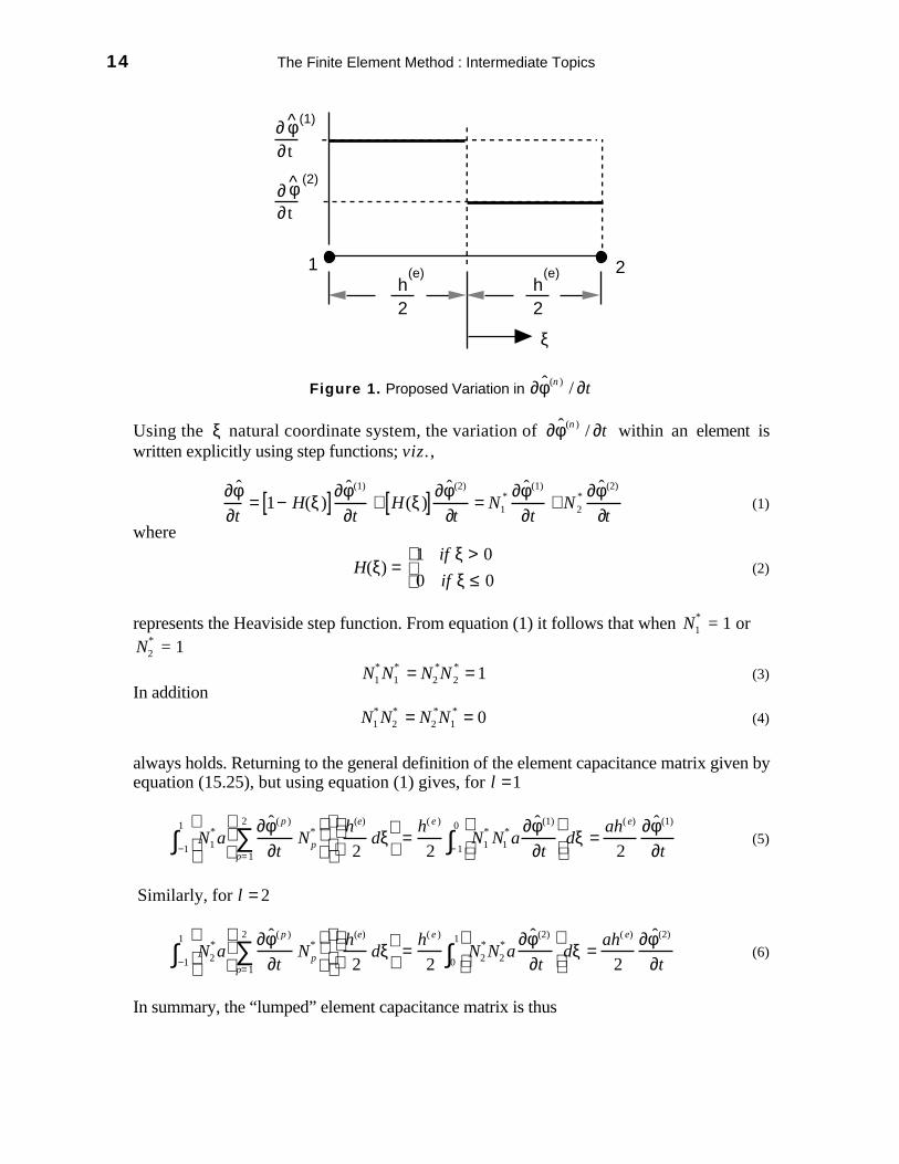
particular, assume that ∂ ˆ φ (n ) / ∂t is constant between the midpoints of adjacent elements.Thus, for a typical element
14 The Finite Element Method : Intermediate Topics
(e)h2
(e)h2
1 2
φ (1)∂∂ t
φ(2)
∂∂ t
ξ
Figure 1. Proposed Variation in ∂ ˆ φ (n ) / ∂t
Using the ξ natural coordinate system, the variation of ∂ ˆ φ (n ) / ∂t within an element iswritten explicitly using step functions; viz. ,
∂ ˆ φ ∂t
= 1− H(ξ)[ ]∂ ˆ φ (1)
∂t+ H(ξ)[ ] ∂ ˆ φ (2)
∂t= N1
* ∂ ˆ φ (1)
∂t+ N2
* ∂ ˆ φ (2)
∂t(1)
where
H(ξ) =1 if ξ > 0
0 if ξ ≤ 0
(2)
represents the Heaviside step function. From equation (1) it follows that when N1* = 1 or
N2* = 1
N1*N1
* = N2*N2
* = 1 (3)In addition
N1*N2
* = N2*N1
* = 0 (4)
always holds. Returning to the general definition of the element capacitance matrix given byequation (15.25), but using equation (1) gives, for l =1
N1*a
∂ ˆ φ ( p )
∂tNp
*
p= 1
2
∑
−1
1
∫h(e)
2dξ
=
h( e )
2N1
* N1*a
∂ ˆ φ (1)
∂t
− 1
0
∫ dξ =ah( e)
2
∂ ˆ φ (1)
∂t(5)
Similarly, for l = 2
N2*a
∂ ˆ φ ( p )
∂tNp
*
p= 1
2
∑
−1
1
∫h(e)
2dξ
=
h( e )
2N2
*N2*a
∂ ˆ φ (2)
∂t
0
1
∫ dξ =ah( e)
2
∂ ˆ φ (2)
∂t(6)
In summary, the “lumped” element capacitance matrix is thus

Chapter 15 : Solution of Transient and Dynamic Problems Using the FEM 15
C( e)[ ]lumped
=ah ( e)
2
1 0
0 1
=
ah(e )
2I[ ] (7)
♦
Using precisely the same procedure described in Chapter 6, the above element equations
will be assembled to form the global set equations
C[ ] ˆ ˙ φ (n ) + K[ ] ˆ φ ( n) + f = 0 (15.32)
where ˆ ˙ φ (n ) ≡∂ ˆ φ ( n)
∂t
, and the last two terms have been combined into the single global load
vector f .

16 The Finite Element Method : Intermediate Topics
15.2.2. Solution Preliminaries
The finite element solution of the first-order transient problem thus results in a set of
coupled ordinary differential equations. Prior to investigating solution strategies for these
equations, some preliminaries need to be discussed.
In general, ˆ ˙ φ (n ) will be approximated using the Finite Difference calculus. To this end,
the time domain is divided into a finite number of intervals
t t t t t t t0 1 2 3 m m+1 nsteps
t = 0
Figure 15.4. Division of the Time Domain into Finite Number of Steps
A typical time step is denoted by
∆tm = tm+1 − tm ; m =1,2,L,(nsteps − 1) (15.33)
The vector of primary dependent variables at time t = tm is denoted by
φ t = tm
= ( m)φ (15.34)
It follows that at t = tm +θ∆tm
φ t = tm +θ
= (m +θ )φ (15.35)
where 0 ≤ θ ≤ 1.
From a suitable Taylor’s series expansion, it can be shown that
( m +θ ) ˙ φ ≅( m +1)φ − ( m )φ
∆tm
(15.36)
which is nothing but a forward difference formula O(∆tm) . In addition, again from a suitable
Taylor’s series expansion,
( m +θ )φ ≅ (1− θ ) (m )φ + θ ( m +1)φ (15.37)

Chapter 15 : Solution of Transient and Dynamic Problems Using the FEM 17
15.2.3. Generalized Trapezoidal Family of One-Step Methods
Evaluating equation (15.32) at t = tm +θ∆tm , and substituting equations (15.36) and
(15.37) gives, upon re-arrangement,
C[ ] +θ∆tm K[ ]( ) ( m +1) ˆ φ n = C[ ] − (1−θ)∆tm K[ ]( ) ( m ) ˆ φ n − ∆tm( m+θ ) f (15.38)
If the same representation is assumed for ( m +θ ) f as for ( m +θ ) ˆ φ (n ) ; viz.,
( m +θ ) f = (1− θ) (m ) f + θ ( m +1) f (15.39)
equation (15.38) then becomes
C[ ] +θ∆tm K[ ]( ) ( m +1) ˆ φ n = C[ ] − (1−θ)∆tm K[ ]( ) ( m ) ˆ φ n −∆tm (1−θ) ( m) f + θ ( m +1) f ( ) (15.40)
Relationships such as equation (15.38) or (15.40) that require only ( m ) ˆ φ n to solve for( m +1) ˆ φ n are classified as “two-level time stepping schemes” or “one-step” methods. In
particular, the algorithms stemming from equation (15.38) or (15.40) are sometimes referred to
as the “generalized trapezoidal family of methods” [2]. Through a suitable choice of the value
of θ , these equations correspond to the following well-known finite difference schemes.
Forward Difference or Forward Euler Scheme
This scheme is realized by setting θ = 0 in equations (15.38) or (15.40), resulting in
C[ ] ( m+1) ˆ φ n = C[ ]− ∆tm K[ ]( ) (m) ˆ φ n −∆ tm(m) f (1)
The scheme is said to be explicit. The benefit of explicit schemes is really only realized ifC[ ] is diagonal (“lumped”). In this case equation (1) is written as
( m +1) ˆ φ n = I[ ] − ∆tm C[ ]−1K[ ]( ) ( m ) ˆ φ n −∆tm C[ ]−1 ( m) f
= ( m ) ˆ φ n − ∆tm C[ ]−1 (m ) f + K[ ] (m) ˆ φ n ( ) (2)
where the inversion of C[ ] is trivial. The computational advantage of such an explicitscheme is accompanied by the disadvantage that, for stability, the magnitude of the timestep ∆tm will be limited. Further details concerning this conditional stability are given inSection 15.2.4.
♦
18 The Finite Element Method : Intermediate Topics
If θ > 0 , a solution scheme is said to be implicit. In this case, a system of equationswith coefficient matrix C[ ] +θ∆tm K[ ]( ) must be solved at each step in order to advance the
solution. If ∆tm , C[ ] and K[ ] remain constant, only one factorization of the coefficient matrix
is necessary. Compared to explicit schemes, implicit ones are more expensive per step but are
more stable. This results in the possibility of using larger time steps in the solution.
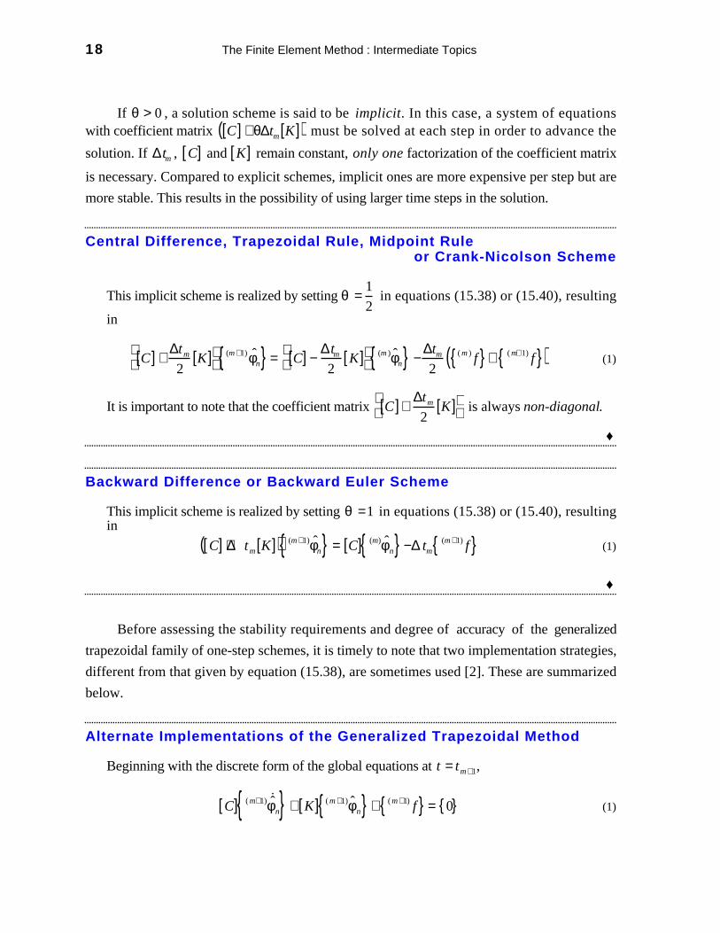
Central Difference, Trapezoidal Rule, Midpoint Ruleor Crank-Nicolson Scheme
This implicit scheme is realized by setting θ =1
2 in equations (15.38) or (15.40), resulting
in
C[ ] +∆tm
2K[ ]
(m +1) ˆ φ n = C[ ] −∆tm2
K[ ]
(m ) ˆ φ n −∆tm
2( m ) f + ( m+ 1) f ( ) (1)
It is important to note that the coefficient matrix C[ ]+∆tm
2K[ ]
is always non-diagonal.
♦
Backward Difference or Backward Euler Scheme
This implicit scheme is realized by setting θ =1 in equations (15.38) or (15.40), resultingin
C[ ] +∆tm K[ ]( ) (m +1) ˆ φ n = C[ ] (m) ˆ φ n −∆ tm(m +1) f (1)
♦
Before assessing the stability requirements and degree of accuracy of the generalized
trapezoidal family of one-step schemes, it is timely to note that two implementation strategies,
different from that given by equation (15.38), are sometimes used [2]. These are summarized
below.
Alternate Implementations of the Generalized Trapezoidal Method
Beginning with the discrete form of the global equations at t = tm +1,
C[ ] ( m+1) ˆ ˙ φ n + K[ ] ( m +1) ˆ φ n + ( m +1) f = 0 (1)

Chapter 15 : Solution of Transient and Dynamic Problems Using the FEM 19
re-write equation (15.36) as
( m +1)φ ≅ (m )φ + ∆tm(m + θ ) ˙ φ (2)
and note that( m +θ ) ˙ φ ≅ (1− θ ) (m) ˙ φ − θ ( m +1) ˙ φ (3)
Applying equations (1) to (3) on the approximate solution, the following twoimplementation strategies have been proposed [2].
“v-Form” of Implementation
At t = t0
C[ ] (0) ˆ ˙ φ n = − K[ ] (0) ˆ φ n − (0) f (4)
where (0) ˆ φ n represents the initial condition. Define the “predictor” of ( m +1) ˆ φ n by
( m +1) ˆ φ n *
= (m +1) ˆ φ n + (1−θ )∆tm( m) ˆ ˙ φ n (5)
Combining equations (2) and (3) gives
( m +1) ˆ φ n = ( m+1) ˆ φ n *
+ θ∆tm(m +1) ˆ ˙ φ n (6)
Substituting equation (6) into (1) gives, upon re-arrangement
C[ ] +θ∆tm K[ ]( ) ( m +1) ˆ ˙ φ n = − ( m+1) f − K[ ] ( m +1) ˆ φ n *
(7)
All terms on the right hand side of equation (7) are known. Once ( m +1) ˆ ˙ φ n has been
determined , ( m +1) ˆ φ n is computed from equation (6). If θ = 0 , the scheme is explicit;
only if C[ ] is diagonal (“lumped”) is the scheme useful, for then the solution may beadvanced without reducing the coefficient matrix. If θ ≠ 0 , the method is implicit; for thesolution to proceed, the coefficient matrix C[ ] +θ∆tm K[ ]( ) must always be reduced.
“d-Form” of Implementation
From equation (6),
( m +1) ˆ ˙ φ n =( m+1) ˆ φ n − ( m +1) ˆ φ n *
θ∆tm(8)

20 The Finite Element Method : Intermediate Topics
Substituting equation (8) into equation (1) gives
1
θ∆tm
C[ ] + K[ ]
(m+ 1) ˆ φ n =
1
θ∆tm
C[ ] ( m +1) ˆ φ n *
− (m +1) f (9)
Once ( m +1) ˆ φ n is determined from equation (9), ( m +1) ˆ ˙ φ n can, if desired, be computed
from equation (6); viz.,
( m +1) ˆ ˙ φ n =( m+1) ˆ φ n − ( m +1) ˆ φ n *
θ∆tm(10)
If C[ ] is diagonal, then the right hand side of equation (9) involves a more accuratedetermination than in the case of equation (7).
♦

Chapter 15 : Solution of Transient and Dynamic Problems Using the FEM 21
15.2.4. Assessment of the Generalized Trapezoidal Method
The primary requirement of the generalized trapezoidal family of one-step schemes is thatthey converge. An algorithm is said to be convergent if, for fixed tm and fixed spatial
discretization, ( m )ˆ φ → (m )φ as ∆tm → 0 .
To establish the convergence of an algorithm, two general topics must be considered,
namely stability (including the study of numerical oscillations) and consistency. It can be
shown that once stability and consistency are verified, convergence is automatic [2].
In addition to studying convergence, the accuracy of the algorithm is also of importance;i.e., the rate of convergence as ∆tm → 0 .
15.2.4.1. Stability
Several techniques may be employed to study the characteristics of an algorithm. In the
present discussion, the commonly used “modal” approach is employed. Returning to the
approximate, discrete form of the governing equations, assume the loading vector to be zero.
As such,
C[ ] ∂ ˆ φ n∂t
+ K[ ] ˆ φ n = 0 (1)
Assume a solution of the form
ˆ φ n = G e− λt(2)
where G represents a vector of (non-zero) constants. Upon substitution of equation (2) into
(1), it follows that
−λ C[ ] + K[ ]( )e− λt = 0 (3)
For a non-trivial solution
det K[ ]− λ C[ ]( ) = 0 (4)
The roots of the resulting polynomial (λp; p =1, 2, . . . , neq) represent the eigenvalues
of the system. If [C] and [K] are positive definite, then the λi are positive and real, with
0 ≤ λ1 ≤ λ 2 ≤ LL≤ λneq (5)
Associated with the λi will be neq eigenvectors

22 The Finite Element Method : Intermediate Topics
ψ i ; i = 1,2,LL,neq(6)
The general solution of equation (1) will thus be a linear combination of exponential
decay terms. If the capacitance matrix possesses the orthonormality property that
ψ i TC[ ] ψ j = δ ij (7)
it follows that
ψ i TK[ ] ψ j = λiδ ij (8)
where δij denotes the Kronecker delta; i.e.,
δ ij =1 if i = j
0 if i ≠ j
(9)
The eigenvectors constitute a basis in ℜneq , meaning that any element in ℜneq can be
written as a linear combination of the eigenvectors; viz. ,
( m ) ˆ φ n = ( m )Yi ψ i i = 1
neq
∑ (10)
and( m +1) ˆ φ n = ( m +1)Yi ψ i
i =1
neq
∑ (11)
In the above equations ( m )Yi and ( m +1)Yi represent “modal participation factors.”
Next consider the approximate discrete form of the equations, with the forward
difference approximation for the first derivative of φ, and with zero forcing
C[ ] +θ∆tm K[ ]( ) ( m +1) ˆ φ n = C[ ] − (1−θ)∆tm K[ ]( ) ( m ) ˆ φ n (12)
Substituting equations (10) and (11) into (12) gives
C[ ] +θ∆tm K[ ]( ) ( m +1)Yi ψ i i =1
neq
∑ = C[ ] − (1−θ )∆tm K[ ]( ) ( m)Yi ψ i i =1
neq
∑ (13)
Pre-multiplication of equation (13) by ψ k T and using the orthonormality relations of
equations (7) and (8) gives

Chapter 15 : Solution of Transient and Dynamic Problems Using the FEM 23
1 +θ∆tmλi( )( m +1)Yi = 1 −(1−θ )∆tmλi( )( m)Yi (14)
or
( m +1)Yi =1 − (1− θ)∆tmλi
1 +θ∆tmλi
( m )Yi =A(m )Yi ; i = 1,2,LL,neq (15)
where
A =1− (1 −θ )∆tmλi
1 + θ∆tmλi
(16)
is called the “amplification factor.” In light of the assumed exponential decay for the solution,
the stability requirement is thus stated as follows:
( m +1)Yi < ( m )Yi for λi > 0( m+ 1)Yi = ( m )Yi for λi = 0
; i = 1,2,LL,neq (17)
From the definition of A, it follows that for λi = 0, A = 1, thus satisfying the second
condition in equation (17). The first condition is equivalent to specifying the inequality A <1
for i = 1, 2, 3, . . . . . ., neq. Put another way,
−1 <1 − (1− θ)∆tmλi
1+ θ∆tmλi
<1 (18)
Recall that for [ C ] and [ K ] positive definite, the eigenvalues shall be positive and real.Also recall that 0 ≤ θ ≤ 1 and that ∆tm > 0. It therefore follows that the right hand inequality
will be satisfied for all values of the parameters. The left hand side of the inequality is satisfied
when
− 1 + θ∆tmλi( ) < 1 − (1− θ)∆tmλi[ ] (19)
or when
−2 < (2θ −1)∆tmλ i[ ] ⇒ θ ≥1
2(20)
regardless of the time step. Such schemes are said to be unconditionally stable. If θ < 0.50,
the left hand inequality requires that
∆tm <2
1− 2θ( )λi
(21)
An algorithm for which stability imposes a time step restriction is called conditionallystable. Equation (21) must hold for all modes; i.e., for λi ; i = 1, 2, . . . . , neq. The greatest

24 The Finite Element Method : Intermediate Topics
λi ; i.e., λneq, imposes the most stringent restriction upon the time step. In large systems of
equations this condition poses a rather severe constraint. As a result, unconditionally stable
algorithms are generally preferred. This is especially true in light of the increased computational
effort once θ > 0 .
Note on Eigenvalues for Stability Assessment
Due to the theorem first stated by Irons and Treharne [7], it is never necessary to obtain theeigenvalues for the global set of equations. This theorem states that the global eigenvaluesare bounded by the eigenvalues of individual elements λ( e ) . In particular
λ j( )min
2≥ λ( e)( )
min
2(1)
and
λ j( )max
2≤ λ(e )( )
max
2(2)
where λ j represents an eigenvalue associated with the global set of equations. The stabilitylimits related to the modal equations are thus ascertained from eigenvalues computed at theelement level.
♦
To get a better idea of the ramifications of unstable algorithms, consider the following
simple example.
Quantification of the Stability Criterion
In general( m +1)Yl = A ( m )Yl (1)
Thus for m = 0,(1)Yl = A (0)Yl (2)
for m = 1(2)Yl = A (1)Yl = A A (0)Yl( ) = A2(0) Yl (3)
Thus, in general, for some m = p
( p+1)Yl = A( p+1) (0)Yl (4)
Assuming a value of (0)Yl =1.0 , the effect of various values of A on the ( m +1)Yl issummarized below.

Chapter 15 : Solution of Transient and Dynamic Problems Using the FEM 25
A ( m +1)Yl
for p = 10
( m +1)Yl
for p = 100
( m +1)Yl
for p = 1000
( m +1)Yl
forp = 10,000
0.90 3.14e-01 2.39e-05 1.57e-46 ~0
0.95 5.69e-01 5.62e-03 5.03e-23 ~0
0.99 8.95e-01 3.62e-01 4.27e-05 2.23e-44
1.01 1.12 2.73 2.12e+04 1.65e+43
1.10 2.85 1.52e+04 2.72e+41 overflow
It is clear that even for a value of A slightly greater than 1.0, the growth in ( m +1)Yl is quitesignificant.
♦
Attention is next focused on the topic of numerical oscillations. That is, the
phenomenon where the calculated results converge to the correct solution, but oscillate around
it. For one time step the calculated value is below the correct value; in the next time step it is
above the correct value. A time marching scheme will be oscillation-free if each modalparticipation factor ( m )Yi has the same sign at each time level m. This can be achieved if from
equation (15)
( m +1)Yi( m )Yi
=1 − (1−θ )∆tmλi
1+θ∆tmλ i
> 0 ; i = 1,2,LL,neq (22)
This is equivalent to requiring that
1 − (1− θ)∆tmλi > 0 (23)
Note that for the backward difference scheme (θ =1), equation (23) is satisfied for anyvalue of the time step ∆tm . For all other values of θ ,
∆tm <1
(1− θ)λi
(24)
For values of ∆tm greater than this, the remaining solution schemes will exhibit oscillation.

26 The Finite Element Method : Intermediate Topics
15.2.4.2. Consistency
In general, denoting the truncation error associated with an algorithm by E(t) , if
E(t) ≤ c ∆tm( )k∀ t > 0 (25)
and if k > 0, the associated algorithm is said to be consistent. In equation (25) c is a constantindependent of ∆tm , and the constant k is termed the order of accuracy or rate of
convergence.
It can be shown that all members of the generalized trapezoidal family of one-step
schemes are consistent [2]. Furthermore, k = 1 ∀ θ ∈[0,1], except for θ =1/ 2 (trapezoidal
rule), in which case k = 2. That is, the trapezoidal rule is second-order accurate.
The above conclusion can be most easily deduced from the truncation error associated
with the Taylor’s series expansion of ( m +θ ) ˙ φ ; viz. ,
( m +θ ) ˙ φ =(m +1)φ −( m )φ
∆tm+ E (26)
where
E =
θ2 − (1−θ )2[ ]∆tm
2( m +θ )˙ φ −
(1−θ)3 + θ3[ ] ∆tm( )2
6( m +θ )˙ φ + LL (27)
From equation (27) it is evident that only the trapezoidal rule (θ =1/ 2 ) is second-order
accurate; i.e., only for θ =1/ 2 does the first term on the right hand side of equation (27)
vanish.

Chapter 15 : Solution of Transient and Dynamic Problems Using the FEM 27
15.3. Solution of Second-Order Dynamic ProblemsUsing Partial Discretization
15.3.1. General Comments
Recall that from Section 15.1.1 that the assumption of partial (semi) discretization leads
to the following general set of matrix equations for the finite element solution of the second-
order dynamic problem:
M ( e )[ ] ˆ ˙ φ n + C ( e)[ ] ˆ ˙ φ n + K (e)[ ] ˆ φ n = f ( e) where
mip( e) = wibNp( )
Ω( e)∫ dΩ
cip( e) = wiaNp( )
Ω (e )∫ dΩ
kip(e ) = − wiL(Np)( )
Ω (e )∫ dΩ
fi(e) = wi f
Ω (e )∫ dΩ
ˆ ˙ φ n ≡∂ 2 ˆ φ n∂t2
and
ˆ ˙ φ n ≡∂ ˆ φ n∂t
We now consider ways in which to solve these equations.
15.3.2. One-Step Algorithms
As noted in the discussion of first-order time-dependent problems, in one-step (or “two
level”) algorithms the solution is based only upon values obtained in the previous step. One-
step algorithms have the advantage that they are self-starting; i.e., a separate starting algorithm
is not required as in the case of multi-step methods (to be discussed in a subsequent section).
Following the notation commonly used in the literature associated with algorithms for solving

28 The Finite Element Method : Intermediate Topics
second-order time-dependent problems, in the sequel let ( m ) ˆ φ n ≡ dm , ( m ) ˆ ˙ φ n ≡ vm , and
( m ) ˆ ˙ φ n ≡ am .
At time t = 0, the state function is defined by the initial conditions
s0 = d0 v0 a0 (15.1)
where the initial accelerations are computed from the equation
Ma0 = f0 − Kd0 − Cv0 (15.2)
If M is diagonal, this solution process is trivial; i.e., no equations need to be solved.At time t = tm > 0 , the state function will be described by
sm = dm vm am (15.3)
Finally, recall that the system matrices possess the following general characteristics: M,
C and K are symmetric; M is positive definite; C and K are, however, positive semi-
definite.
15.3.2.1. The Newmark Family of Algorithms
The Newmark integration scheme is based on the following assumptions regarding the
velocity and displacement increments [Newmark 1959]
vm +1 = vm +∆ tm (1−γ )am + γ am+1[ ] (15.4)
dm +1 = dm +∆ tmvm + (∆tm )2 1
2− β
am + βam +1
(15.5)
In addition, the equations of dynamic equilibrium
Mam +1 + Cvm +1 + Kdm +1 = fm +1 (15.6)
must be satisfied.
In the above equations β and γ represent parameters whose values must be selected such
as to obtain stability and integration accuracy. Stability implies that if, for example, a small

Chapter 15 : Solution of Transient and Dynamic Problems Using the FEM 29
(incremental) increase in d0 is introduced, the response will only change by a small
(incremental) amount.
The parameter γ controls algorithmic damping. Values of γ > 0.50 introduce algorithmic
damping or amplitude decay (see Figure 15.???); γ = 0.50 introduces no algorithmic damping;
and, values of γ < 0.50 introduce growth (clearly undesirable).
-1.0
-0.5
0.0
0.5
1.0
0.0 2.0 4.0 6.0 8.0 10.0 12.0
true responseartificially decayed response
Re
spo
nse
Time
Figure 15.???. Schematic Illustration of Amplitude Decay
The parameter β controls stability. Unconditional stability is assured if β ≥ 0.50γ . In
light of the above observations, it follows that practically speaking 2β ≥ γ ≥1
2.
On the subject of accuracy, it has been shown that for the case of γ =1
2 (i.e., no
algorithmic damping), the Newmark schemes are second-order accurate [2]. If γ >1
2, the
accuracy reduces to first-order.
Turning attention to the implementation of the Newmark schemes, the following two
approaches have been advocated [2].

30 The Finite Element Method : Intermediate Topics
“a-form” Implementation of the Newmark Algorithm [2]
First the following “predictors” are defined
˜ d m +1 ≡ dm +∆ tmvm + (∆tm )2 1
2− β
am (1)
˜ v m +1 ≡ vm +∆ tm(1− γ ) am (2)It follows that
dm +1 = ˜ d m +1 + (∆tm)2β am +1 (3)
vm +1 = ˜ v m +1 +γ (∆tm )am + 1 (4)
Substituting equations (3) and (4) into the equation of motion (15.6) gives
Ma m+1 + C ˜ v m +1 + ∆tmγ am +1[ ] + K ˜ d m + 1 + (∆tm )2β am +1[ ] = fm+1 (5)
orM +∆tmγ C + (∆tm)2 β K[ ]am +1 = fm+1 − C˜ v m + 1 − K˜ d m + 1
(6)
Unless both M and C are diagonal and β = 0, the algorithm will be implicit.
♦
“d-form” Implementation of the Newmark Algorithm [2]
From equation (15.5) it follows that
am +1 =1
β1
(∆tm )2 dm +1 − dm( ) −1
∆tm
vm −1
2− β
am
(1)
Substituting equation (1) into (15.4) gives
vm +1 = vm +∆ tm (1− γ )am +γ∆tm
β1
(∆tm )2 dm +1 − d m( ) −1
∆tmvm −
1
2− β
am
(2)
Finally, substituting equations (1) and (2) into the equation of motion (15.6) leads to
1
β(∆tm )2 M +γ
β∆tm
C + K
dm+1 = fm +1 +1
βM
1
(∆tm )2 dm +1
∆tm
vm +1
2− β
am

Chapter 15 : Solution of Transient and Dynamic Problems Using the FEM 31
−C vm + ∆tm(1− γ )am −γ∆tm
β1
(∆tm )2 dm +1
∆tm
vm +1
2− β
am
(3)
♦
Some examples of specific members of the Newmark family of methods are next
presented.
Average Acceleration Method
This scheme, in which β =1
4 and γ =
1
2, was proposed by Newmark in his original paper
[ref]. For this method, equations (15.4) and (15.5) become
vm +1 = vm +∆tm
2am + am +1[ ] (1)
dm +1 = dm +∆ tmvm +(∆tm )2
4am + am +1[ ] (2)
Since β ≠ 0 the algorithm is implicit. In addition, since β ≥ γ / 2 , the algorithm is
unconditionally stable. Finally, since γ =1
2, the algorithm is second-order accurate.
♦
Linear Acceleration Method
In this scheme β =1
6 and γ =
1
2, thus specializing equations (15.4) and (15.5) to
vm +1 = vm +∆tm
2am + am +1[ ] (1)
dm +1 = dm +∆ tmvm +(∆tm )2
62 am + am +1[ ] (2)
Since β ≠ 0 the algorithm is implicit. Since γ =1
2, the algorithm is second-order
accurate. Finally, the algorithm is conditionally stable. The requirement for stability is that[2]
∆tm ≤3
πTmin =
2 3
ω max
(3)
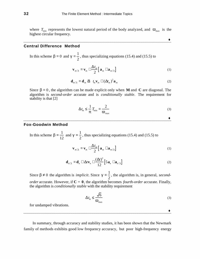
32 The Finite Element Method : Intermediate Topics
where Tmin represents the lowest natural period of the body analyzed, and ωmax is thehighest circular frequency.
♦
Central Difference Method
In this scheme β = 0 and γ =1
2, thus specializing equations (15.4) and (15.5) to
vm +1 = vm +∆tm
2am + am +1[ ] (1)
dm +1 = dm +∆ tmvm + (∆tm )2am (2)
Since β = 0 , the algorithm can be made explicit only when M and C are diagonal. Thealgorithm is second-order accurate and is conditionally stable. The requirement forstability is that [2]
∆tm ≤1
πTmin =
2
ω max
(3)
♦
Fox-Goodwin Method
In this scheme β =1
12 and γ =
1
2, thus specializing equations (15.4) and (15.5) to
vm +1 = vm +∆tm
2am + am +1[ ] (1)
dn+1 = dn + ∆tvn +(∆t)2
125an +an +1[ ] (2)
Since β ≠ 0 the algorithm is implicit. Since γ =1
2, the algorithm is, in general, second-
order accurate. However, if C = 0 , the algorithm becomes fourth-order accurate. Finally,the algorithm is conditionally stable with the stability requirement
∆tm ≤6
ωmax
(3)
for undamped vibrations.
♦
In summary, through accuracy and stability studies, it has been shown that the Newmark
family of methods exhibits good low frequency accuracy, but poor high-frequency energy

Chapter 15 : Solution of Transient and Dynamic Problems Using the FEM 33
dissipation. The latter phenomenon is a result of the spatial discretization of the solution
domain [2]. It has been shown that for implicit members of the Newmark family with γ >1
2,
taking β =1
4γ +
1
2
2
will maximize the high frequency dissipation [2].
15.3.2.2. Hilber-Hughes-Taylor Method (α-method)
The Hilber-Hughes-Taylor (HHT) scheme is referred to as an “optimal collocation
method” [9]. In this scheme the finite difference formulas associated with the Newmark
“family” of algorithms are retained; viz. ,
dm +1 = dm +∆ tmvm + (∆tm )2 1
2− β
am + βam +1
(1)
vm +1 = vm +∆ tm (1−γ )am + γ am+1[ ] (2)
However, the time-discrete equation of motion is modified as follows
Mam +1 + (1+ α )Cvm +1 − α Cvm + (1+ α )Kdm +1 − αKdm = fm +α (3)
wheretm+ α = (1+ α)tm +1 − α tm = tm + 1 +α∆tm (4)
From equation (3) it is evident that the HHT scheme is self-starting.
Concerning the numerical implementation of the HHT scheme, begin with the definition
of the “predictors”; viz. ,
˜ d m +1 ≡ dm +∆ tmvm + (∆tm )2 1
2− β
am (5)
˜ v m +1 ≡ vm +∆ tm(1− γ ) am (6)
Equations (1) and (2) thus become
dm +1 = ˜ d m +1 + (∆tm)2β am +1 (7)
vm +1 = ˜ v m +1 +γ (∆tm )am + 1 (8)
From equation (7)

34 The Finite Element Method : Intermediate Topics
am +1 =dm+1 − ˜ d m +1
β (∆tm )2 (9)
Substituting equation (9) into equation (8) gives
vm +1 = ˜ v m +1 +γ (dm + 1 − ˜ d m +1)
β(∆tm)(10)
Finally, substituting equations (9) and (10) into equation (3) gives, after some
manipulation
1
β(∆tm )2 M +(1+ α)γβ(∆tm)
C + (1+ α )K
dm +1
= fm + α +1
β(∆tm)2 M˜ d m +1 −(1+ α )C ˜ v m +1 −γ
β(∆tm )˜ d m +1
+ α Cvm + αKdm (11)
An unconditionally stable, second-order algorithm is realized if [2]
α ∈ −1
3,0
; γ =1
2(1− 2α ) ; β =
1
4(1−α )2 (12)
If α = 0 and γ =1
2= 2β , the HHT scheme reduces to the “d-form” implementation of
the average acceleration method, only with f = fn . Decreasing α increases the amount of
numerical dissipation. Finally, the scheme has been shown to provide a good combination
between low-frequency accuracy and high-frequency dissipation [2].

Chapter 15 : Solution of Transient and Dynamic Problems Using the FEM 35
15.3.3. Multi-Step Algorithms
On the subject of multi-step algorithms, Zienkiewicz and Taylor [14] state that:
“Such algorithms are in general less convenient to use than the single-stepprocesses as they do not permit an easy change of the time step magnitude.However, much classical work on stability and accuracy has been introduced onsuch multistep algorithms and hence they deserve a mention.”
Consequently, a select number of multi-step algorithms are described below.
The Houbolt Method
The Houbolt integration scheme [11] is related to the central difference method in that
standard finite difference expressions are used to approximate the acceleration and velocity
components in terms of displacement components.
The following finite difference expansions are employed
vn+1 =1
6(∆t)11dn +1 −18dn + 9dn−1 − 2dn− 2( ) (1)
an+1 =1
(∆t )2 2dn+1 − 5dn + 4dn−1 − dn− 2( ) (2)
Equations (1) and (2) represent two backward difference formulas with truncation errors
O(∆t )2 . These equations are supplemented by the equation of dynamic equilibrium
Man+1 + Cvn+1 + Kdn+1 = fn+1 (3)
Substitution of equations (1) and (2) into (3) gives, after some manipulation, the
following equation
2
(∆t)2 M +11
6∆tC + K
dn+1 = fn +1 +
5
(∆t)2 M +3
∆tC
dn
−4
(∆t)2 M +3
2∆tC
dn−1 +
1
(∆t)2 M +1
3∆tC
dn −2 (4)
From equation (4) it is evident that even if M and C are diagonal, the method will be implicit.

36 The Finite Element Method : Intermediate Topics
Equation (4) implies the need for a special starting procedure to compute the solutions d1
and d2 (d0 is known from the initial conditions). One common approach is to use a different
integration scheme for the first two time steps. This “starting” scheme should preferably be
unconditionally stable, though a conditionally stable one (e.g., the central difference scheme
with a fraction of the “safe” ∆t employed) could likewise be used.
The Houbolt method is unconditionally stable. It exhibits very good high-frequency
dissipation, but “poor” second-order accuracy [2].
♦

Chapter 15 : Solution of Transient and Dynamic Problems Using the FEM 37
15.4. Notes Concerning Mass Matrices
A mass matrix is a discrete representation of the continuous distribution of mass in a
body. Although seemingly a straightforward issue, the development of mass matrices has, in
the past, been realized using different approaches. These approaches, and the associated
strengths and limitations are discussed in this section. Additional information can be found in
the books of Cook et al. [3], Hughes [2], and Zienkiewicz and Taylor [4].
15.4.1. Consistent Mass Matrices
As noted in Section 15.1, the element mass matrix is computed from
M ( e )[ ] = N[ ]Tb N[ ]
Ω( e )∫ dΩ (1)
where now b ≡ ρ denotes the mass density [units of ML-3] of the material comprising the
element. Since equation (1) employs the same interpolation functions as the rest of the
discretization, the associated mass matrix is termed consistent. As noted by Zienkiewicz and
Taylor [4]:
“The name of ‘consistent mass matrix’ has been coined . . . . , a term whichmay be considered to be unnecessary since it is the logical and naturalconsequence of the discretization process.”
Consistent mass matrices are symmetric and generally full. When assembled, they havethe same sparse topology as K ( e )[ ] . When ρ is non-zero, consistent mass matrices are
positive definite; i.e., the kinetic energy
1
2ˆ ˙ φ n T
M( e)[ ] ˆ ˙ φ n is positive for any non-zero ˆ ˙ φ n . In addition, consistent mass matrices have been shown to
lead to optimal error estimates [2].
15.4.2. Lumped Mass Matrices
In the infancy of dynamic finite element analyses, the mass of the elements was usually
arbitrarily “lumped” at the nodes, even if no actual concentrated masses existed. Consequently,

38 The Finite Element Method : Intermediate Topics
the resulting mass matrices were always diagonal. In general, for a given displacement degreeof freedom, the lumping procedure places particle masses m j at each node j of an element. The
only requirement of such “lumping” is that the total mass be conserved; i.e.,
m jj = 1
N en
∑ = ρ dΩΩ (e )∫ (2)
where N en denotes the total number of nodes in the element, and an irreducible formulation is
implied. Unless it is arbitrarily assigned (e.g., for the rotational degrees of freedom associated
with flexural elements, plates and/or shells), the mass “lumps” have no rotary inertia. As noted
by Zienkiewicz and Taylor [4], the fact that the lumping procedure was unnecessary and
apparently inconsistent was independently recognized by Archer [12] and by Leckie and
Lindberg [13].
Although for rather simple elements mass lumping is somewhat intuitive, for high-order
elements and/or for elements possessing irregular geometries, more systematic approaches are
necessary. A few of the more commonly used approaches are now described.
Diagonalization Employing Alternate Interpolation Functions
This approach was used earlier in this chapter to derive the lumped element capacitancematrix for the two-node heat conduction element. Practically speaking, the approach is onlyapplicable to simple elements. It consists of replacing the consistent mass matrix, withentries given by
mij( e ) = Ni ρN j
Ω( e)∫ dΩ (1)
with the matrix containing the entries
m ij( e ) = Ni
* ρN j*
Ω( e)∫ dΩ (2)
where the Ni* represent piecewise constant, non-overlapping functions defined over the
entire element such that Ni* = 1 at node i, and Ni
* = 0 at all other nodes. Such anapproximation with different interpolation functions is permissible provided that the usualfinite element criteria of integrability and completeness are satisfied [14]. Since nodifferentiation is involved in equation (2), it suffices for the Ni
* to be piecewise constantand non-overlapping. In addition, the usual condition of
Ni*
i =1
N en
∑ =1 (3)
must be satisfied.

Chapter 15 : Solution of Transient and Dynamic Problems Using the FEM 39
The benefit of using an ad-hoc lumping approach employing alternate interpolationfunctions is that the nodal masses shall be positive. The drawback of such an approach isthat the accuracy of the associated dynamic analysis will be sub-optimal [3,20].Consequently, for all but the simplest elements, other mass lumping approaches musttypically be adopted.
♦
Diagonalization Employing the Row-Sum Method
In this approach the entries of the lumped element mass matrix are given by
m ii
( e ) = mij(e )
j =1
N en
∑ ; i = 1,2,L, Nen (1)
where the mij( e ) are the values computed for a consistent mass matrix, and no summation
over repeated indices is implied. The row-sum technique sometimes produces negativemasses (e.g., for the corner nodes of the 8-node Serendipity quadrilateral element). Underaxisymmetric conditions, non-zero masses are obtained along the axis of symmetry.
Programming Note:
In general
mij( e ) = Ni ρN j
Ω( e)∫ dΩ (2)
For the row-sum method, for each translational degree of freedom
m ii( e ) = mij
(e )
j =1
N en
∑ = Ni ρN j
Ω (e )∫ dΩ
j =1
Nen
∑
= Ni ρ N jj =1
Nen
∑
Ω( e )∫ dΩ = Ni
Ω (e )∫ ρ dΩ (3)
which represents a reduction in computational effort as compared to that associated with thecomputation of consistent mass matrices.
♦
Diagonalization Employing Diagonal Scaling [15-17]
The general idea behind diagonal scaling is: set the entries of the lumped element massmatrix proportional to the diagonal entries of the consistent element mass matrix; viz. ,
m ii( e ) = cmii
( e) ; i =1,2,L, Nen (1)
where c is a scalar determined using consistent mass values and the criterion of massconservation. In particular, the following steps are used to apply this scheme [3]:

40 The Finite Element Method : Intermediate Topics
(1) Compute only the diagonal coefficients of the consistent mass matrix. Due to thepositive definiteness of the consistent mass matrix, these entries are necessarilypositive.
(2) Compute the total mass M of the element.
(3) Compute a scalar constant c by adding the diagonal coefficients mii( e ) associated only
with translational degrees of freedom that are in the same direction.
(4) Scale all the diagonal coefficients by multiplying them by the ratio M / c , thuspreserving the total mass of the element.
The most important attribute of the diagonal scaling scheme is that it always producespositive lumped masses.
To date, it has been shown that for flexural and low-order continuum elements in structuraland solid mechanics applications, the accuracy of lumped mass matrices obtained usingdiagonal scaling is excellent, often surpassing that of the consistent mass matrices [3]. Inaddition, optimal rates of convergence are often realized [2].
For higher-order elements, this scheme may be less accurate for transient analyses than anoptimally lumped mass matrix [18,19]. The subject of optimally lumped mass matrices isdiscussed next.
♦
Diagonalization Employing Nodal Quadrature
Mass lumping can also be realized by applying an appropriate quadrature rule to evaluatethe element mass matrix [20,21]. If the integration locations associated with a quadraturerule coincide with nodal locations of an element having only translational degrees offreedom, then no off-diagonal terms are generated. If, however, the element also hasrotational degrees of freedom, then lumping by nodal quadrature produces block-diagonalmatrices. Since these are no longer diagonal, they have rather limited practical usefulness[3].
Addressing the issue of optimal lumping, let p = the degree of the highest order completepolynomial in N[ ] , and let m = the highest order derivative in the strain energy expression.Then a quadrature rule with degree of precision of 2( p − m) will yield comparable accuracyand incur no loss of convergence rate beyond that already inherent in the finite elementanalysis with consistent mass matrices. Diagonal mass matrices integrated in this way aresaid to be optimally lumped. These conditions are sufficient but may not be necessary[22].
Note Concerning Axisymmetric Idealizations
In axisymmetric analyses, the use of nodal quadrature produces zero masses at nodes lyingalong the axis of symmetry; i.e., along the x2 - or z -axis. This can be better understood bynoting that in general,
M ( e )[ ] = 2π N[ ]T ρ N[ ]rdrdzΩ( e)∫ (1a)

Chapter 15 : Solution of Transient and Dynamic Problems Using the FEM 41
≈ 2π N(ξn ,ηn )[ ]Tρ N(ξn ,ηn)[ ]rnwn (1b)
where n ranges from 1 to the total number of quadrature points, and wn represents aquadrature weight. Since along the axis of symmetry r = 0 , the mass at those nodes islikewise zero.
Optimal Quadrature Rules for Lagrange Elements
As discussed by Hughes [2], the nodal locations of Lagrange Elements coincide with theintegration locations of Lobatto quadrature. Lobatto quadrature weights are alwayspositive. Consequently, optimal lumping for Lagrange elements always results in positivedefinite, diagonal element mass matrices.
In order to obtain positive nodal masses in cubic and higher-order Lagrange elements, thenodes in the reference elements must be located at special positions [18].
Optimal Quadrature Rules for Serendipity Quadrilateralsand Triangular Elements
In general, it is not possible to construct an integration rule of a required accuracy thatsimultaneously permits arbitrary specification of integration locations and has positiveweighting [3]. Thus, optimally lumped diagonal mass matrices for serendipityquadrilaterals and triangular elements, particularly quadratic and higher-order, have somezero or negative nodal masses.
♦
Example : 2-node bar element
In order to illustrate the above lumping techniques, consider a linear two-node bar elementfor two-dimensional analysis 3.
1u
, Ae
x1
x2
1
2 (2)
u(1)
2
u(1)
1
u 2(2)
e
Ee
Typical Linear Bar Element in 2-Space
3 Further details concerning bar elements are given in Chapter 14.

42 The Finite Element Method : Intermediate Topics
Consistent Mass Matrix
The interpolation functions associated with this element are
N1 =1
2(1− ξ) ; N2 =
1
2(1+ ξ ) (1)
The consistent element mass matrix is thus computed in the following manner
M ( e )[ ] = N[ ]T ρ ( e) N[ ]Ω( e )∫ dΩ= N[ ]T ρ (e ) N[ ]A( e ) h( e )
2dξ
−1
1
∫ (2a)
=ρ (e ) A(e)h( e )
2
N1 0
0 N1
N2 0
0 N2
N1 0 N2 0
0 N1 0 N2
dξ
−1
1
∫ (2b)
=ρ (e ) A(e)h( e )
2
N1N1 0 N1N2 0
0 N1N1 0 N1N2
N1N2 0 N2N2 0
0 N1N2 0 N2N2
dξ−1
1
∫ (2c)
=ρ (e ) A(e)h( e )
6
2 0 1 0
0 2 0 1
1 0 2 0
0 1 0 2
(2d)
where ρ( e) , A(e ) and h (e ) represent the mass density, constant cross-sectional area, andlength, respectively, of the element. From equation (2d), it is evident that, with respect toeach of the two coordinate directions, mass is being conserved.
Diagonalization Employing Alternate Interpolation Functions
The following, alternate, interpolation functions are used
N1* = 1− H(ξ) ; N2
* = H(ξ) (3)where
H(ξ) =1 if ξ > 0
0 if ξ ≤ 0
(4)
represents the Heaviside step function.

Chapter 15 : Solution of Transient and Dynamic Problems Using the FEM 43
(e)h2
ξ
1
0
N1*
ξ
1
0
N2*
(e)h2
(e)h2
(e)h2
Alternate Interpolation Functions
Since when N1* = 1 or N2
* = 1
N1*N1
* = N2*N2
* = 1 (5)And since
N1*N2
* = N2*N1
* = 0 (6)
always holds, it follows that
N1* N1
* dξ−1
1
∫ = dξ−1
0
∫ =1 (7)
and
N2* N2
* dξ−1
1
∫ = dξ0
1
∫ = 1 (8)
Replacing N1 and N2 by N1* and N2
* in equation (2), respectively, the diagonal elementmass matrix is thus
M ( e)[ ] =ρ( e )A ( e)h( e )
2
1 0 0 0
0 1 0 0
0 0 1 0
0 0 0 1
(9)
Diagonalization Employing the Row-Sum Method
For the element under consideration, N sdim = 2 and Neddof = 4. Thus, for each translationaldegrees of freedom
m ii( e ) = mij
(e )
j =1
4
∑ ; i = 1,2 (10)
where mij( e ) represents the (i, j) th entry in the consistent element mass matrix. Then for
i =1,

44 The Finite Element Method : Intermediate Topics
m 11( e ) = m1 j
( e)
j =1
4
∑ =ρ( e )A(e )h( e)
62 + 0 + 1 + 0( ) =
ρ( e )A ( e)h( e )
2(11)
Similarly,
m 22( e ) = m 33
( e) = m 44( e ) =
ρ( e )A( e)h(e )
2(12)
The resulting element mass matrix is thus identical to that obtained using alternateinterpolation functions. This is a fairly common occurrence for lower-order elements.
Diagonalization Employing Diagonal Scaling
The four steps described above are followed, namely: (1) The diagonal entries of M ( e )[ ]have been determined above; (2) The total mass of the element is equal to M = ρ (e) A(e)h( e ) ;(3) For the degrees of freedom parallel to the global x1 coordinate direction, and likewisefor the degrees of freedom parallel to the global x2 coordinate direction, the scalar constantis
c = m11( e ) + m22
( e) =ρ( e) A( e )h(e)
62 + 2( ) =
2
3ρ( e) A( e )h (e)
(13)
(4) for rows 1 and 3, and likewise for rows 2 and 4,
M / c =ρ (e )A( e)h( e )
23
ρ( e )A(e )h(e )=
3
2(14)
Thus
m 11( e ) =
3
2
2ρ (e ) A( e)h(e )
6
=
ρ (e) A(e )h( e)
2= m 33
( e )(15)
and
m 22( e ) =
3
2
2ρ (e ) A( e)h(e )
6
=
ρ (e) A(e )h( e)
2= m 44
( e )(16)
The resulting element mass matrix is thus identical to that obtained using alternateinterpolation functions.
Diagonalization Employing Nodal Quadrature
For this element, p = 1 and m = 1, thus 2( p − m) = 0. Consequently, the quadratureformula need only integrate constants exactly. The simplest such formula that uses thenodes as quadrature points is the Trapezoidal rule (i.e., the Closed Newton-Cotes formulafor n = 1); viz. ,

Chapter 15 : Solution of Transient and Dynamic Problems Using the FEM 45
f (x) dx ≈x0
x1
∫x1 − x0
2
f(x0) + f (x1 )[ ] (17)
Thus, noting that x1 − x0
2
=
1 − (−1)
2=1 ,
M ( e)[ ] = N[ ]T ρ( e ) N[ ]− 1
1
∫ A( e ) h(e )
2dξ
(18a)
≈ρ (e) A(e )h ( e)
2N[ ]T
N[ ]( )ξ =−1
+ N[ ]TN[ ]( )
ξ= 1
(18b)
Since
N[ ]TN[ ] =
N1 0
0 N1
N2 0
0 N2
N1 0 N2 0
0 N1 0 N2
=
N1N1 0 N1N2 0
0 N1N 0 N1N2
N1N2 0 N2N2 0
0 N1N2 0 N2N2
(19)
where N1 =1
2(1− ξ) and N2 =
1
2(1+ ξ ), it follows that
N1N1 =1
4(1− ξ)2 =
1 for ξ =−1
0 for ξ = +1
(20)
N1N2 =1
4(1− ξ 2) =
0 for ξ = −1
0 for ξ = +1
(21)
N2N2 =1
4(1+ ξ )2 =
0 for ξ = −1
1 for ξ = +1
(22)
Thus
M ( e)[ ] =ρ( e )A ( e)h( e )
2
1 0 0 0
0 1 0 0
0 0 1 0
0 0 0 1
(23)
The resulting element mass matrix is thus again identical to that obtained using the otherlumping schemes.
♦

46 The Finite Element Method : Intermediate Topics
15.4.3. Concluding Remarks Concerning Consistentand Diagonal Mass Matrices
In summary of the previous two sections concerning consistent and diagonal mass
matrices, the following conclusions have been reached:
• Neither lumped or consistent mass matrices are best for all problems.
• For low-order elements such as the linear bar, the constant strain (linear) triangle, and bi-linear quadrilaterals, ad hoc lumping usually gives identical results as optimal lumping [3].
• For the quadratic Lagrange element, diagonal scaling and optimal quadrature lumpingproduce the same diagonal element mass matrix [3]. For cubic and higher-order Lagrangeelements, diagonal scaling and optimal quadrature lumping may produce different results[3].
• For quadratic and higher-order triangular and serendipity quadrilateral elements, diagonalscaling and optimal quadrature lumping are markedly different. The results of numericaltests on certain problems [18,19] indicate that the displacement, velocity and accelerationtime-history results for diagonal scaling models can be less accurate than for ones usingoptimal quadrature lumping [3].
In assessing the rate of convergence, and thus order of accuracy, of the various mass
matrices, use is typically [2] made of the relation 4
ˆ ω ω
−1 ≤ chm(1)
whereˆ ω = circular frequency associated with the discrete system;
ω = exact circular frequency;
h = a typical element dimension;
c = a constant independent of h ; and,
m = a constant that quantifies the order of accuracy or rate of convergence
From equation (1) it follows that
lnˆ ω
ω−1 = ln c + m lnh (2)
Since h is inversely proportional to the number of elements N e, ln h( ) = − ln Ne( ) , and
4 Recall the discussion of consistency presented in Section 15.2.4.2.

Chapter 15 : Solution of Transient and Dynamic Problems Using the FEM 47
lnˆ ω
ω−1 = ln c − m ln Ne( ) (3)
The order of accuracy is thus represented as the negative of the slope of a lnˆ ω
ω−1 vs.
ln Ne( ) diagram.
15.4.4. Higher-Order Mass Matrices
As discussed by Hughes [2], the consistent mass matrix is not always the best non-
diagonal mass matrix. In certain cases, non-diagonal mass matrices exhibiting superior
accuracy to the consistent mass have been developed. However, at present no general theory
for obtaining such higher-order mass matrices is available [2].
EXAMPLE : Linear Rod Element
For the linear two-node bar element considered previously in this chapter, the consistentand diagonal element mass matrix have been shown to be
M ( e )[ ] =ρ (e )A ( e)h( e )
6
2 1
1 2
(1)
and
M ( e)[ ] =ρ( e )A ( e)h( e )
2
1 0
0 1
(2)
respectively. The following higher-order mass matrix has been proposed by Goudreau [23]
˜ M ( e )[ ] =ρ (e )A ( e)h( e )
12
5 1
1 5
(3)
For uniform meshes, this element mass matrix leads to fourth-order accurate frequencies,
as compared to the second-order accurate M ( e )[ ] and M ( e)[ ] . ˜ M ( e )[ ] can be obtained by
simply averaging M ( e )[ ] and M ( e)[ ] ; viz. ,
˜ M ( e )[ ] =1
2M ( e)[ ] + M (e )[ ]( ) (4)
As noted by Hughes [2], ˜ M ( e )[ ] can be derived in the following, alternate, manner
˜ M ( e )[ ] = M (e)[ ] +1
6− r
ρ (e ) h ( e)( )2
E(e ) K ( e)[ ] (5a)

48 The Finite Element Method : Intermediate Topics
=ρ (e ) A(e)h( e )
6
2 1
1 2
+
1
6− r
ρ
(e )A (e )h( e)1 −1
−1 1
(5b)
For r =1
12, the general expression gives
˜ M ( e )[ ] =ρ (e )A ( e)h( e )
6
2 1
1 2
+
ρ( e)A( e )h( e)
12
1 −1
−1 1
=
ρ( e )A (e)h( e)
12
5 1
1 5
(6)
which corresponds to the matrix proposed by Goudreau [23]. If r = 0 , equation (4) gives
˜ M ( e )[ ] =ρ (e )A ( e)h( e )
6
2 1
1 2
+
ρ( e)A( e )h( e)
6
1 −1
−1 1
=
ρ( e )A (e)h( e)
2
1 0
0 1
(7)
which is the diagonal element mass matrix. Finally, if r =1
6, ˜ M ( e )[ ] simply reduces to the
consistent element mass matrix.
♦
EXAMPLE : Bernoulli-Euler (Hermite Cubic) Beam Element
For a Bernoulli-Euler beam element without axial degrees of freedom, such as that shownbelow
3,1
(2)(1)
3,11 2
h(e)
u(1)
3
(2)
3u
ρ(e) (e), A-u -u
(e), I
Typical Bernoulli-Euler Beam Element
the consistent and lumped (via trapezoidal rule) mass matrices can be shown to be
M ( e )[ ] =ρ (e )A ( e)h( e )
420
156 22h( e ) 54 −13h(e )
22h( e) 4h( e )2 13h ( e) −3h( e )2
54 13h( e ) 156 −22h( e)
−13h(e ) −3h( e )2 −22h( e) 4h(e) 2
(1)
and

Chapter 15 : Solution of Transient and Dynamic Problems Using the FEM 49
˜ M ( e )[ ] =ρ (e )A ( e)h( e )
2
1 0 0 0
0 0 0 0
0 0 1 0
0 0 0 0
(2)
respectively. In equation (2), the rotary inertia has been neglected. The higher-orderelement mass matrix associated with the above Bernoulli-Euler beam element is derivedfrom the following expression [24]
˜ M ( e )[ ] = M (e)[ ] +αρ (e )A( e) h( e )( )4
E (e )I ( e) K ( e )[ ] (3)
For a uniform mesh, the value of α = 1/ 720 has been shown to lead to sixth-orderaccurate frequencies [2].
♦

50 The Finite Element Method : Intermediate Topics
15.5. Notes Concerning Damping Matrices
Recall that damping enters the discrete formulation through the consistent element
damping matrix
C( e)[ ] = N[ ]Ta N[ ]dΩ
Ωe∫
which is predicated upon the assumption of viscous damping. However, damping in structures
is known not to be viscous, but is due to mechanisms such as hysteresis in the material
response, slip in connections, energy dissipation due to cracking, etc. None the less, in the
interest of keeping the equations computationally simple, viscous damping is assumed [25].
In general, the treatment of damping in computational dynamic analyses can be
categorized as being based upon [3]: (1) Phenomenological representations in which actual
dissipative mechanisms are modeled; and/or, (2) Spectral damping methods in which viscous
damping is introduced by means of specified fractions of critical damping.
The element and system damping matrices can be consistent or they can be diagonal
(lumped). The difficulty comes in defining the viscous terms a .Since the cost of analyses is significantly increased if C( e)[ ] and thus C[ ] are not banded,
in most practical analyses using direct integration, C[ ] is often assumed to be a linear
combination of the global mass and stiffness matrices; viz. ,
C[ ] = α M[ ] + β K[ ]
where the constants α and β are determined experimentally 5. Such damping is known as
Rayleigh damping, and represents a popular spectral damping scheme. In structures with
widely varying material properties (e.g., soil-structure interaction problems), different values
of α and β may need to be assigned to different parts of the solution domain.
For modal superposition analyses, orthogonal damping matrices are highly desirable.
Such matrices can be computed using the approach proposed by Wilson and Penzien [26].
Diagonal damping matrices, required for explicit solutions, can be determined using the
notion of a weighted modal matrix, formed from the columns of eigenvectors for the global
system of equations [27].
5 To a large extent, the magnitudes of α and β are determined by the energy dissipation characteristics of the
structural materials associated with the problem.

Chapter 15 : Solution of Transient and Dynamic Problems Using the FEM 51
15.6. Exercises
Exercise 15.1. : one-dimensional transient heat conduction analysis
Consider the insulated rod of unit cross-sectional area shown below.
L
x
insulated
insulated
The associated (parabolic) governing differential equation is
ρc∂T
∂t= k
∂ 2T
∂x2
with initial conditionsT (x, 0) = T0 ∀ 0 < x < L
and boundary conditions
T (0, t) = T (L,t) = 0.0 ∀ t > 0
The exact solution to this problem is
T (x,t) =
4T0
nπsin
nπx
Ln=1,3,5,L
∞
∑ e−n2 π 2 kt
ρcL2
Concerning the numerical solution, for simplicity, initially use a four element mesh with:
• L = 8.0 cm
• Material properties: k = 2.0 W/cm-oC and ρc = 6.0 J/cm3-oC
Please do the following:
(a) Using hand computations, determine the system conductivity matrix K and the system
capacitance matrix C (both consistent and “lumped”).
(b) Realizing that, due to the Dirichlet boundary condition at x = 0 and x = L, the first row
and column of these matrices will be modified/eliminated, consider only the resulting 3x 3 sub-matrices. Determine the eigenvalues (0 ≤ λ1 ≤ λ2 ≤ λ3 ) and eigenvectors Ψ1, Ψ2
, Ψ3 associated with this “reduced” problem. Do this for both the consistent and

52 The Finite Element Method : Intermediate Topics
“lumped” capacitance matrices and compare the eigenvalues associated with the two
cases6.
(c) Using the equations developed in lecture to determine a value of ∆t such that the
computations will be stable and oscillation free, determine the smallest values of timestep ∆tn for use with:
1) The forward difference method (θ = 0);
2) The central difference or Crank-Nicolson method (θ = 0.5); and,
3) The backward difference method (θ = 1.0).
Do this for both the consistent and “lumped” formulations.
(d) Code up the problem for analysis using the T1DHC computer program. Then, using thevalues of ∆tn determined in part (c) above, analyze the problem to at least 100 seconds.
(e) On a single graph for each value of θ, plot temperature versus distance along the rod at t
= ∆tn (i.e., at the first time step), 2∆tn , ~20, ~40, ~60 and ~100 seconds. Analyze the
results obtained (compare them with the exact solution) and comment on your findings.
Do this for both the consistent and “lumped” formulations.
(f) Finally, using a value of ∆tn = 3.0 seconds, and the forward difference method (θ = 0),
repeat part (d). Do this for the consistent formulation only. Comment on your findings.
6 NOTE: this task can easily be accomplished by using MATLAB, or similar program. The
procedure to be followed for MATLAB is:
1) Enter the matrices [C] and [K] in the usual manner.2) Then issue the command: [X,D] = eig(K,C)
This produces a diagonal matrix [D] of eigenvalues and a full matrix [X] whose columnsare the corresponding eigenvectors.

Chapter 15 : Solution of Transient and Dynamic Problems Using the FEM 53
Exercise 15.2. : axial vibration of a uniform bar
Consider a quadratic, three-node bar element
(1)u
ξ
,
1 2 3
E(e)
A(e)
(e)0.5 h
(e)0.5 h
(2)u
(3)u
The associated interpolation functions are
N1 =ξ2
(ξ −1) ; N2 = (1− ξ 2 ) ; N3 =ξ2
(ξ +1)
Recall that the element stiffness matrix is given by
K ( e )[ ] =A( e )E( e)
3h
7 −8 1
−8 16 −8
1 −8 7
where E (e ) denotes the elastic modulus and A(e ) is the cross-sectional area.
(a) The consistent element mass matrix for the element is given by
M ( e )[ ] =ρ (e )A ( e)h( e )
30
4 2 −1
2 16 2
−1 2 4
where ρ( e) denotes the mass density. Using this information, determine the following
element mass matrices using:
(a.1) The diagonal (“lumped”) element mass matrix obtained using the row-summethod.
(a.2) The diagonal (“lumped”) element mass matrix obtained using the diagonal scaling(or HRZ) scheme.
(a.3) The diagonal (“lumped”) element mass matrix obtained using the optimalquadrature (which in this case is Simpson’s rule).
(a.4) The average of the consistent mass matrix and that obtained using optimalquadrature.

54 The Finite Element Method : Intermediate Topics
(a.5) The diagonal (“lumped”) element mass matrix obtained using an “ad hoc”lumping in which particles of mass equal to ρAh / 3 are placed at each node.
(b) Next consider the axial vibration of an unsupported, elastic, uniform bar of length L and
total mass ρAL . The exact natural frequencies for the bar are
ω i =
iπL
E
ρ; i = 0,1,2, L
Using three node bar elements, model the bar by first using one element, and then by using
two elements of equal size (i.e., h (e ) = L / 2 ). In each case, compute the lowest threeapproximate natural frequencies ( ˆ ω 1, ˆ ω 2 , ˆ ω 3 ; ˆ ω 1 < ˆ ω 2 < ˆ ω 3 ) and compare them with the
exact values. Do this using the consistent element matrix, and the diagonal matrices
determined in parts (b.3), (b.4) and (b.5) above. What is the physical significance of the
lowest mode ? For the second and third modes, represent your results in a plot of lnˆ ω ω
−1
as the ordinate versus the natural logarithm of the number of elements. You will thus have a
line for each mass matrix used for each of the two (second and third) modes.
In your analyses, assume E = 30.0 x10⁶ , A = 4.0 , L = 50 and ρ = 150.
NOTE: the eigenvalues and associated eigenvectors are determined form the characteristicequation
det K[ ]− ω 2 M[ ]( ) = 0
Consequently, the eigenvalues obtained using standard numerical schemes (e.g.,MATLAB) represent the squares of the natural frequencies.

Chapter 15 : Solution of Transient and Dynamic Problems Using the FEM 55
15.7. References
1 . S. J. Farlow, Partial Differential Equations for Scientists and Engineers, J. Wiley andSons, New York (1982).
2 . T. J. R. Hughes, The Finite Element Method, Linear Static and Dynamic FiniteElement Analysis, Prentice-Hall, New Jersey (1987).
3 . R. D. Cook, D. S. Malkus and M. E. Plesha, Concepts and Applications of FiniteElement Analysis, 3rd ed., J. Wiley & Sons, New York (1989).
4 . O. C. Zienkiewicz and R. L. Taylor, The Finite Element Method, Fourth Edition,Volume 2, McGraw-Hill, New York (1991).
5 . K. J. Bathe, Finite Element Procedures, Prentice Hall, New Jersey (1996).
6 . K. Terzaghi, Erdbaumechanik auf Bodenphysikalischer Grundlage, Franz Deuticke,Leipzig und Wien, Vienna (1925).
7 . B. M. Irons and C. Treharne, “A bound theorem for eigenvalues and its practicalapplications,” in 2nd Conference on Matrix Methods in Structural Mechanics, Wright-Pattersen AFB, Dayton, Ohio (1971), 245-254.
8 . N. M. Newmark, “A Method of Computation for Structural Dynamics,” Journal of theEngineering Mechanics Division, ASCE, 85(EM3) (1959), 67-94.
9 . H. M. Hilber, T. J. R. Hughes and R. L. Taylor, “Improved Numerical Dissipation forTime Integration Algorithms in Structural Dynamics,” Earthquake Engineering andStructural Dynamics, 5(3) (1977), 283-292.
10. E. L. Wilson, I. Farhoomand and K. J. Bathe, “Nonlinear Dynamic Analysis of ComplexStructures,” International Journal of Earthquake Engineering and Structural Dynamics,1 (1973), 241-252.
11. J. C. Houbolt, “A Recurrence Matrix Solution for the Dynamic Response of ElasticAircraft,” Journal of Aeronautical Science, 17(9) (1950), 540-550.
12. J. S. Archer, “Consistent Mass Matrix for Distributed Systems,” Proceedings of theAmerican Society of Civil Engineers, 89 , ST4 (1963), 161-178.
13. F. A. Leckie and G. M. Lindberg, “The Effect of Lumped Parameters on BeamFrequencies,” Aeronautics Quarterly, 14 (1963), 224-240.
14. O. C. Zienkiewicz and R. L. Taylor, The Finite Element Method, Fourth Edition,Volume 1, McGraw-Hill (1989).
15. S. W. Key and Z. E. Beisinger, “The Transient Dynamic Analysis of This Shells in theFinite Element Method,” Proceedings of the 3rd Conference on Matrix Methods andStructural Mechanics, Wright-Patterson AFB, Ohio (1971).

56 The Finite Element Method : Intermediate Topics
16. E. Hinton, A. Rock and O. C. Zienkiewicz, “A Note on Mass Lumping and RelatedProcesses in the Finite Element Method,” Earthquake Engineering and StructuralDynamics, 4(3) (1976), 245-249.
17. K. S. Surana, “Lumped Mass Matrices with Non-Zero Inertia for Geneal Shell andAxisymmetric Shell Elements,” International Journal for Numerical Methods inEngineering, 12(11) (1978), 1635-1650.
18. D. S. Malkus and M. E. Plesha, “Zero and Negative Masses in Finite Element Vibrationand Transient Analysis,” Computer Methods in Applied Mechanics and Engineering,59(3) (1986), 281-306.
19. D. S. Malkus, M. E. Plesha and M. R. Liu, “Reversed Stability Conditions in TransientFinite Element Analysis,” Computer Methods in Applied Mechanics and Engineering,68(1) (1988), 97-114.
20. P. Tong, T. H. H. Pian and L. L. Bociovelli, “Mode Shapes and Frequencies by theFinite Element Method Using Consistent and Lumped Matrices,” Computers andStructures, 1 (1971), 623-638.
21. I. Fried and D. S. Malkus, “Finite Element Mass Matrix Lumping by NumericalIntegration with No Convergence Rate Loss,” International Journal of Solids andStructures, 11(4) (1975), 461-466.
22. G. J. Fix, “Effects of Quadrature Errors in Finite Element Approximation of Steady State,Eigenvalue and Parabolic Problems,” in Mathematical Foundations of the FiniteElement Method with Applications to Partial Differential Equations, I. Babuska andA. K. Aziz, eds., Academic Press, New York (1972), 525-556.
23. G. L. Goudreau, “Evaluation of Discrete Methods for the Linear Dynamic Response ofElastic and Viscoelastic Solids, UC SESM Report 69-15 , UC Berkeley (1970).
24. R. L. Taylor and R. Iding, “Application of Extended Variational Principles to FiniteElement Analysis,” in Variational Methods in Engineering, 1 , Southampton UniversityPress (1973), 2.54-2.67.
25. R. W. Clough and J. Penzien, Dynamics of Structures, McGraw-Hill, New York(1975).
26. E. L. Wilson and J. Penzien, “Evaluation of Orthogonal Damping Matrices,”International Journal of Numerical Methods in Engineering, 4 (1972), 5-10.
27. W. T. Thomson, T. Calkins and P. Caravani, “A Numerical Study of Damping,”Earthquake Engineering and Structural Dynamics, 3 (1974), 97-103.

Chapter 15 : Solution of Transient and Dynamic Problems Using the FEM 57
15.8. Suggested Reading
K. J. Bathe, Finite Element Procedures, Prentice Hall, New Jersey (1996).
R. D. Cook, D. S. Malkus and M. E. Plesha, Concepts and Applications of Finite ElementAnalysis, 3rd ed., J. Wiley & Sons, New York (1989).
O. C. Zienkiewicz and K. Morgan, Finite Elements and Approximation, J. Wiley & Sons,New York (1983).