Solution of Problems in Heat Transfer Transient Conduction

1

Solution of Problems in Heat Transfer

Transient Conduction or Unsteady

Conduction

Author

Assistant Professor: Osama Mohammed Elmardi

Mechanical Engineering Department

Faculty of Engineering and Technology

Nile Valley University, Atbara, Sudan

First Edition: April 2017

2

Solution of Problems in Heat Transfer

Transient Conduction or Unsteady

Conduction

Author

Assistant Professor: Osama Mohammed Elmardi




First Edition: April 2017

ii

Dedication

In the name of Allah, the merciful, the compassionate

All praise is due to Allah and blessings and peace is upon his messenger and

servant, Mohammed, and upon his family and companions and whoever follows his

guidance until the day of resurrection.

To the memory of my mother Khadra Dirar Taha, my father Mohammed

Elmardi Suleiman, and my dear aunt Zaafaran Dirar Taha who they taught me the

greatest value of hard work and encouraged me in all my endeavors.

To my first wife Nawal Abbas and my beautiful three daughters Roa, Rawan

and Aya whose love, patience and silence are my shelter whenever it gets hard.

To my second wife Limya Abdullah whose love and supplication to Allah were

and will always be the momentum that boosts me through the thorny road of research.

To Professor Mahmoud Yassin Osman for reviewing and modifying the

manuscript before printing process.

This book is dedicated mainly to undergraduate and postgraduate students,

especially mechanical and production engineering students where most of the

applications are of mechanical engineering nature.

To Mr. Osama Mahmoud of Daniya Center for publishing and printing services

whose patience in editing and re – editing the manuscript of this book was the

momentum that pushed me in completing successfully the present book.

To my friend Professor Elhassan Mohammed Elhassan Ishag, Faculty of

Medicine, University of Gezira, Medani, Sudan.

To my friend Mohammed Ahmed Sambo, Faculty of Engineering and

Technology, Nile Valley University, Atbara, Sudan.

iii

To my homeland, Sudan, hoping to contribute in its development and

superiority.

Finally, may Allah accept this humble work and I hope that it will be beneficial

to its readers

iv

Acknowledgement

I am grateful and deeply indebted to Professor Mahmoud Yassin Osman for

valuable opinions, consultation and constructive criticism, for without which this

work would not have been accomplished.

I am also indebted to published texts in thermodynamics and heat and mass

transfer which have been contributed to the author's thinking. Members of

Mechanical Engineering Department at Faculty of Engineering and Technology, Nile

Valley University, Atbara – Sudan, and Sudan University of Science & Technology,

Khartoum – Sudan have served to sharpen and refine the treatment of my topics. The

author is extremely grateful to them for constructive criticisms and valuable

proposals.

I express my profound gratitude to Mr. Osama Mahmoud and Mr. Ahmed

Abulgasim of Daniya Center for Printing and Publishing services, Atbara, Sudan

who they spent several hours in editing, re – editing and correcting the present

manuscript.

Special appreciation is due to the British Council's Library for its quick response

in ordering the requested bibliography, books, reviews and papers.

v

Preface

During my long experience in teaching several engineering subjects I noticed

that many students find it difficult to learn from classical textbooks which are written

as theoretical literature. They tend to read them as one might read a novel and fail to

appreciate what is being set out in each section. The result is that the student ends his

reading with a glorious feeling of knowing it all and with, in fact, no understanding of

the subject whatsoever. To avoid this undesirable end a modern presentation has been

adopted for this book. The subject has been presented in the form of solution of

comprehensive examples in a step by step form. The example itself should contain

three major parts, the first part is concerned with the definition of terms, the second

part deals with a systematic derivation of equations to terminate the problem to its

final stage, the third part is pertinent to the ability and skill in solving problems in a

logical manner.

This book aims to give students of engineering a thorough grounding in the

subject of heat transfer. The book is comprehensive in its coverage without

sacrificing the necessary theoretical details.

The book is designed as a complete course test in heat transfer for degree

courses in mechanical and production engineering and combined studies courses in

which heat transfer and related topics are an important part of the curriculum.

Students on technician diploma and certificate courses in engineering will also find

the book suitable although the content is deeper than they might require.

The entire book has been thoroughly revised and a large number of solved

examples and additional unsolved problems have been added. This book contains

comprehensive treatment of the subject matter in simple and direct language.

The book comprises eight chapters. All chapters are saturated with much needed

text supported and by simple and self-explanatory examples.

Chapter one includes general introduction to transient conduction or unsteady

conduction, definition of its fundamental terms, derivation of equations and a wide

spectrum of solved examples.

vi

In chapter two the time constant and the response of temperature measuring

devices were introduced and discussed thoroughly. This chapter was supported by

different solved examples.

Chapter three discusses the importance of transient heat conduction in solids

with finite conduction and convective resistances. At the end of this chapter a wide

range of solved examples were added. These examples were solved using Heisler

charts.

In chapter four transient heat conduction in semi – infinite solids were

introduced and explained through the solution of different examples using Gaussian

error function in the form of tables and graphs.

Chapter five deals with the periodic variation of surface temperature where the

periodic type of heat flow was explained in a neat and regular manner. At the end of

this chapter a wide range of solved examples was introduced.

Chapter six concerns with temperature distribution in transient conduction. In

using such distribution, the one dimensional transient heat conduction problems could

be solved easily as explained in examples.

In chapter seven additional examples in lumped capacitance system or negligible

internal resistance theory were solved in a systematic manner, so as to enable the

students to understand and digest the subject properly.

Chapter eight which is the last chapter of this book contains unsolved theoretical

questions and further problems in lumped capacitance system. How these problems

are solved will depend on the full understanding of the previous chapters and the

facilities available (e.g. computer, calculator, etc.). In engineering, success depends

on the reliability of the results achieved, not on the method of achieving them.

I would like to express my appreciation of the assistance which I have received

from my colleagues in the teaching profession. I am particularly indebted to Professor

Mahmoud Yassin Osman for his advice on the preparation of this textbook.

When author, printer and publisher have all done their best, some errors may

still remain. For these I apologies and I will be glad to receive any correction or

constructive criticism.

vii

Assistant Professor/ Osama Mohammed Elmardi Suleiman




February 2017

viii

Contents

Subject Page

Number

Dedication ii

Acknowledgement iv

Preface v

Contents viii

CHAPTER ONE : Introduction

1.1 General Introduction 2

1.2 Definition of Lumped Capacity or Capacitance System 3

1.3 Characteristic Linear Dimensions of Different Geometries 3

1.4 Derivations of Equations of Lumped Capacitance System 5

1.5 Solved Examples 7

CHAPTER TWO : Time Constant and Response of Temperature

Measuring Instruments

2.1 Introduction 17


CHAPTER THREE : Transient Heat Conduction in Solids with Finite

Conduction and Convective Resistances

3.1 Introduction 25


CHAPTER FOUR : Transient Heat Conduction in Semi – Infinite Solids

4.1 Introduction 38

4.2 Penetration Depth and Penetration Time 42


CHAPTER FIVE : Systems with Periodic Variation of Surface Temperature

5.1 Introduction 51


ix

CHAPTER SIX : Transient Conduction with Given Temperatures

6.1 Introduction 55


CHAPTER SEVEN : Additional Solved Examples in Lumped Capacitance

System

7.1 Example (1) Determination of Temperature and Rate of Cooling

of a Steel Ball

58

7.2 Example (2) Calculation of the Time Required to Cool a Thin

Copper Plate

59

7.3 Example (3) Determining the Conditions Under which the

Contact Surface Remains at Constant Temperature

62

7.4 Example (4) Calculation of the Time Required for the Plate to

Reach a Given Temperature

63

7.5 Example (5) Determination of the Time Required for the Plate to


64

7.6 Example (6) Determining the Temperature of a Solid Copper

Sphere at a Given Time after the Immersion in a Well – Stirred Fluid

65

7.7 Example (7) Determination of the Heat Transfer Coefficient 66

7.8 Example (8) Determination of the Heat Transfer Coefficient 67

7.9 Example (9) Calculation of the Initial Rate of Cooling of a Steel

Ball

69

7.10 Example (10) Determination of the Maximum Speed of a

Cylindrical Ingot Inside a Furnace

70

7.11 Example (11) Determining the Time Required to Cool a Mild

Steel Sphere, the Instantaneous Heat Transfer Rate, and the Total

Energy Transfer

71

7.12 Example (12) Estimation of the Time Required to Cool a

Decorative Plastic Film on Copper Sphere to a Given Temperature

using Lumped Capacitance Theory

73

x

7.13 Example (13) Calculation of the Time Taken to Boil an Egg 75

7.14 Example (14) Determining the Total Time Required for a

Cylindrical Ingot to be Heated to a Given Temperature

76

CHAPTER EIGHT : Unsolved Theoretical Questions and Further Problems

in Lumped Capacitance System

8.1 Theoretical Questions 80

8.2 Further Problems 80

References 86

Appendix: Mathematical Formula Summary 89

1

Chapter One

Introduction

From the study of thermodynamics, you have learned that energy can be

transferred by interactions of a system with its surroundings. These interactions are

called work and heat. However, thermodynamics deals with the end states of the

process during which an interaction occurs and provides no information concerning

the nature of the interaction or the time rate at which it occurs. The objective of this

textbook is to extend thermodynamic analysis through the study of transient

conduction heat transfer and through the development of relations to calculate

different variables of lumped capacitance theory.

In our treatment of conduction in previous studies we have gradually considered

more complicated conditions. We began with the simple case of one dimensional,

steady state conduction with no internal generation, and we subsequently considered

more realistic situations involving multidimensional and generation effects. However,

we have not yet considered situations for which conditions change with time.

We now recognize that many heat transfer problems are time dependent. Such

unsteady, or transient problems typically arise when the boundary conditions of a

system are changed. For example, if the surface temperature of a system is altered,

the temperature at each point in the system will also begin to change. The changes

will continue to occur until a steady state temperature distribution is reached.

Consider a hot metal billet that is removed from a furnace and exposed to a cool air

stream. Energy is transferred by convection and radiation from its surface to the

surroundings. Energy transfer by conduction also occurs from the interior of the

metal to the surface, and the temperature at each point in the billet decreases until a

steady state condition is reached. The final properties of the metal will depend

significantly on the time – temperature history that results from heat transfer.

Controlling the heat transfer is one key to fabricating new materials with enhanced

properties.

2

Our objective in this textbook is to develop procedures for determining the time

dependence of the temperature distribution within a solid during a transient process,

as well as for determining heat transfer between the solid and its surroundings. The

nature of the procedure depends on assumptions that may be made for the process. If,

for example, temperature gradients within the solid may be neglected, a

comparatively simple approach, termed the lumped capacitance method or negligible

internal resistance theory, may be used to determine the variation of temperature with

time.

Under conditions for which temperature gradients are not negligible, but heat

transfer within the solid is one dimensional, exact solution to the heat equation may

be used to compute the dependence of temperature on both location and time. Such

solutions are for finite and infinite solids. Also, the response of a semi – infinite solid

to periodic heating conditions at its surface is explored.

1.1 General Introduction:

Transient conduction is of importance in many engineering aspects for an

example, when an engine is started sometime should elapse or pass before steady

state is reached. What happens during this lap of time may be detrimental. Again,

when quenching a piece of metal, the time history of the temperature should be

known (i.e. the temperature – time history). One of the cases to be considered is when

the internal or conductive resistance of the body is small and negligible compared to

the external or convective resistance.

This system is also called lumped capacity or capacitance system or negligible

internal resistance system because internal resistance is small, conductivity is high

and the rate of heat flow by conduction is high and therefore, the variation in

temperature through the body is negligible. The measure of the internal resistance is

done by the Biot (Bi) number which is the ratio of the conductive to the convective

resistance.

𝑖. 𝑒. 𝐵𝑖 = ℎ𝑙

𝑘

3

When 𝐵𝑖 ≪ 0.1 the system can be assumed to be of lumped capacity (i.e. at Bi =

0.1 the error is less than 5% and as Bi becomes less the accuracy increases).

1.2 Definition of Lumped Capacity or Capacitance System:

Is the system where the internal or conductive resistance of a body is very small

or negligible compared to the external or convective resistance.

Biot number (Bi): is the ratio between the conductive and convective resistance.

𝐵𝑖 = ℎ𝑙

𝑘 → 𝐵𝑖 =

𝑐𝑜𝑛𝑑𝑢𝑐𝑡𝑖𝑜𝑛 𝑟𝑒𝑠𝑖𝑠𝑡𝑎𝑛𝑐𝑒

𝑐𝑜𝑛𝑣𝑒𝑐𝑡𝑖𝑜𝑛 𝑟𝑒𝑠𝑖𝑠𝑡𝑎𝑛𝑐𝑒=

𝑥

𝑘𝐴/

1

ℎ𝐴=

𝑥

𝑘𝐴×

ℎ𝐴

1=

ℎ𝑥

𝑘

Where 𝑥 is the characteristic linear dimension and can be written as 𝑙, ℎ is the heat

transfer coefficient by convection and k is the thermal conductivity.

When 𝐵𝑖 ≪ 0.1 , the system is assumed to be of lumped capacity.

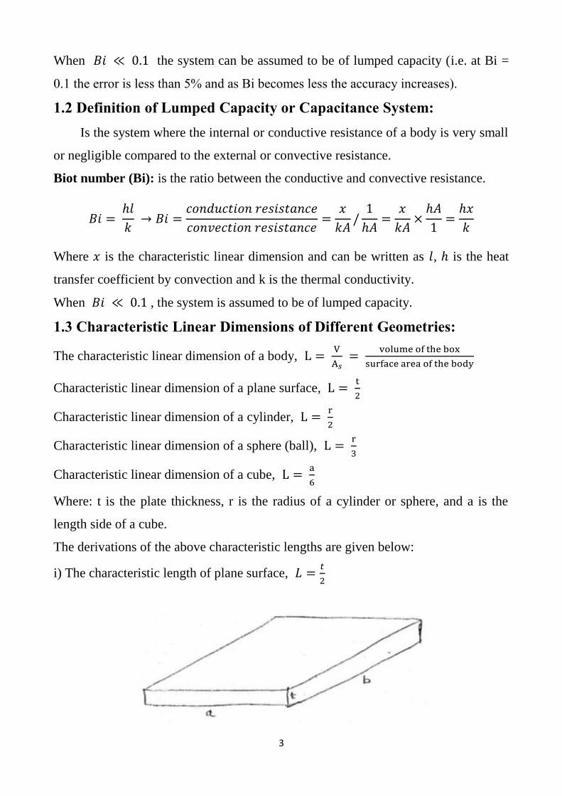
1.3 Characteristic Linear Dimensions of Different Geometries:

The characteristic linear dimension of a body, L = V

A𝑠 =

volume of the box

surface area of the body

Characteristic linear dimension of a plane surface, L = t

2

Characteristic linear dimension of a cylinder, L = r

2

Characteristic linear dimension of a sphere (ball), L = r

3

Characteristic linear dimension of a cube, L = a

6

Where: t is the plate thickness, r is the radius of a cylinder or sphere, and a is the

length side of a cube.

The derivations of the above characteristic lengths are given below:

i) The characteristic length of plane surface, 𝐿 =𝑡

2

4

𝑉 = 𝑎𝑏𝑡

𝐴𝑠 = 2𝑎𝑡 + 2𝑏𝑡 + 2𝑎𝑏

Since, t is very small; therefore, it can be neglected.

𝐴𝑠 = 2𝑎𝑏

𝐿 =𝑉

𝐴𝑠=

𝑎𝑏𝑡

2𝑎𝑏=

𝑡

2

ii) The characteristic length of cylinder,

𝐿 =𝑉

𝐴𝑠=

𝑟

2

𝑉 = 𝜋𝑟2𝐿

𝐴𝑠 = 2𝜋𝑟𝐿

∴ 𝐿 =𝑉

𝐴𝑠=

𝜋𝑟2𝐿

2𝜋𝑟𝐿=

𝑟

2

iii) The characteristic length of a sphere (ball),

𝐿 =𝑟

3

𝑣 =4

3𝜋𝑟3

𝐴𝑠 = 4𝜋𝑟2

∴ 𝐿 =𝑉

𝐴𝑠=

43

𝜋𝑟3

4𝜋𝑟2=

𝑟

3

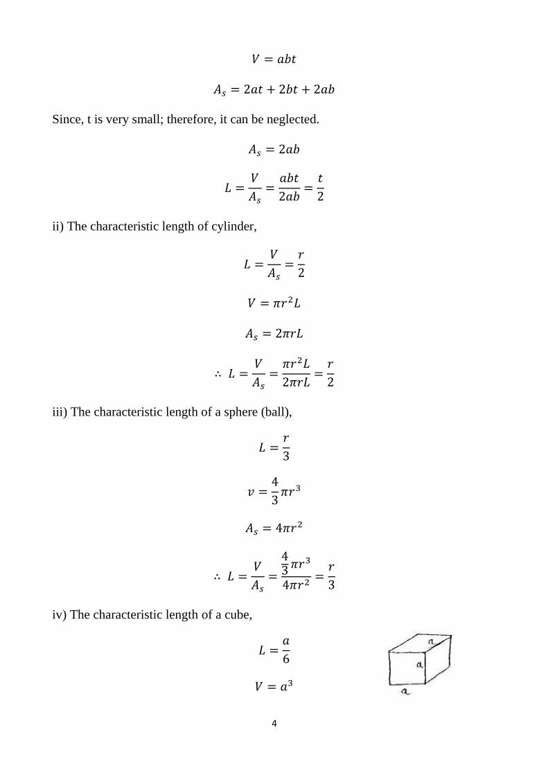
iv) The characteristic length of a cube,

𝐿 =𝑎

6

𝑉 = 𝑎3

5

𝐴𝑠 = 6𝑎2

𝐿 =𝑉

𝐴𝑠=

𝑎3

6𝑎2=

𝑎

6

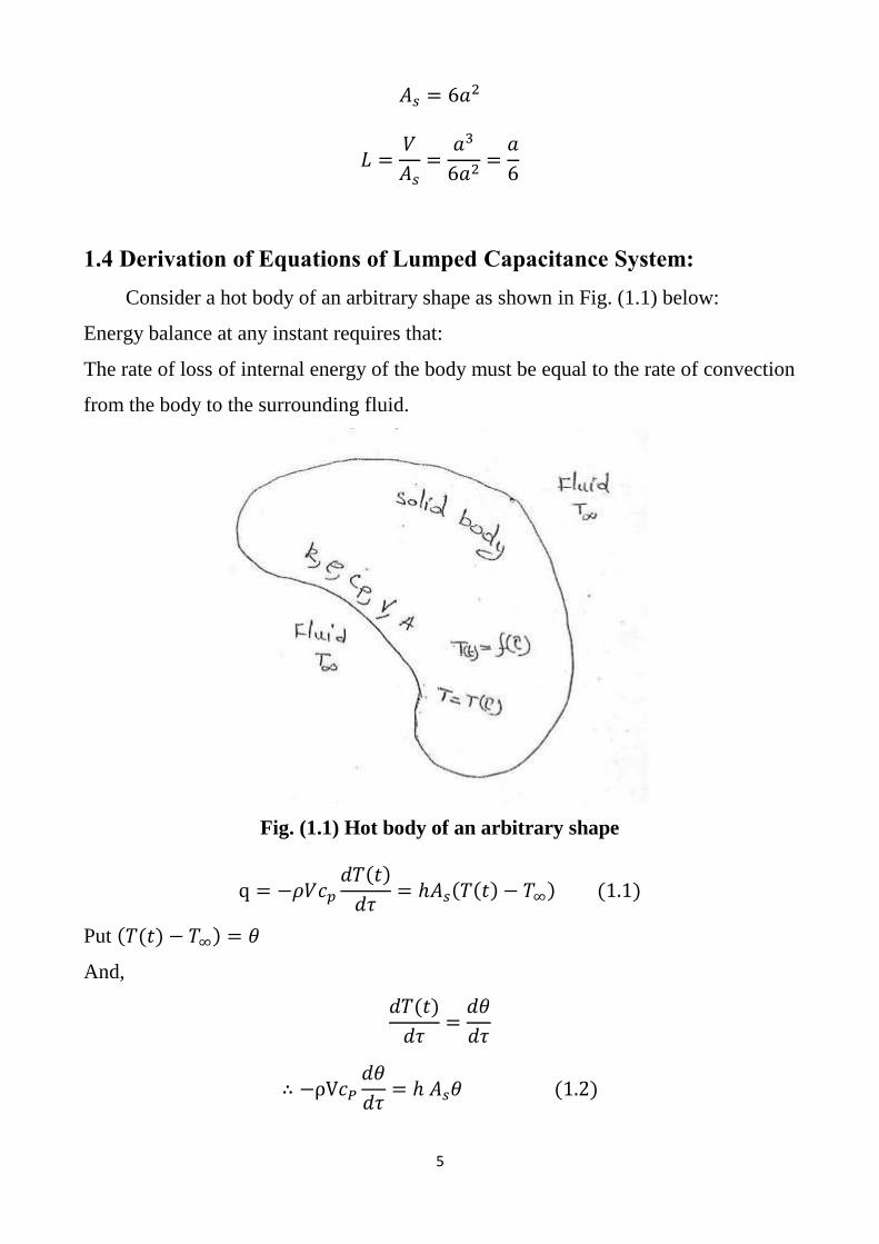
1.4 Derivation of Equations of Lumped Capacitance System:

Consider a hot body of an arbitrary shape as shown in Fig. (1.1) below:

Energy balance at any instant requires that:

The rate of loss of internal energy of the body must be equal to the rate of convection

from the body to the surrounding fluid.

Fig. (1.1) Hot body of an arbitrary shape

q = −𝜌𝑉𝑐𝑝

𝑑𝑇(𝑡)

𝑑𝜏= ℎ𝐴𝑠(𝑇(𝑡) − 𝑇∞) (1.1)

Put (𝑇(𝑡) − 𝑇∞) = 𝜃

And,

𝑑𝑇(𝑡)

𝑑𝜏=

𝑑𝜃

𝑑𝜏

∴ −ρV𝑐𝑃

𝑑𝜃

𝑑𝜏= ℎ 𝐴𝑠𝜃 (1.2)

6

If the temperature of the body at time 𝜏 = 0 is equal to 𝑇𝑜

∴ 𝜃𝑜 = 𝑇𝑜 − 𝑇∞

−𝜌𝑉𝑐𝑃

𝑑𝜃

𝜃= ℎ𝐴𝑠 𝑑𝜏 (1.3)

By integrating the above equation (1.3) we obtain the following equation:

−𝜌𝑉𝑐𝑃 ∫𝑑𝜃

𝜃= ∫ ℎ𝐴𝑠 𝑑𝜏

𝜏=𝜏

𝜏=0

𝜃

𝜃𝑜

−𝜌𝑉 ln𝜃

𝜃𝑜= ℎ𝐴𝑠 𝜏

ln𝜃

𝜃𝑜= −

ℎ𝐴𝑠 𝜏

𝜌𝑉𝑐𝑃

∴ 𝜃

𝜃𝑜= 𝑒

−ℎ𝐴𝑠 𝜏𝜌𝑉𝑐𝑃 (1.4)

ℎ𝐴𝑠

𝜌𝑉𝑐𝑃∙ 𝜏 can be written as

ℎ 𝑉

𝑘𝐴𝑠∙

𝐴𝑠2𝑘

𝑉2𝜌𝑐𝑃𝜏 (1.5)

𝑘

𝜌𝑐𝑃𝐿2∙ 𝜏 = Fourier number Fo (dimensionless Quantity) (1.6)

And,

ℎ 𝐿

𝑘= 𝐵𝑖 (1.7)

∴ ℎ𝐴𝑠

𝜌𝑉𝑐𝑃∙ 𝜏 = 𝐵𝑖 × 𝐹𝑜 (1.8)

∴ 𝜃

𝜃𝑜=

𝑇(𝑡) − 𝑇∞

𝑇𝑜 − 𝑇∞= 𝑒−𝐵𝑖×𝐹𝑜 (1.9)

The instantaneous heat transfer rate 𝑞′(𝜏) is given by the following equation:

𝑞′(𝜏) = ℎ𝐴𝑠𝜃 = ℎ𝐴𝑠𝜃𝑜𝑒−𝐵𝑖×𝐹𝑜 (1.10)

At time 𝜏 = 0,

7

𝑞′(𝜏) = ℎ𝐴𝑠𝜃𝑜 (1.11)

The total heat transfer rate from 𝜏 = 0 to 𝜏 = 𝜏 is given by the following equation:

𝑄(𝑡) = ∫ 𝑞′(𝜏) = ∫ ℎ𝐴𝑠𝜃𝑜𝑒−𝐵𝑖×𝐹𝑜𝜏

0

𝜏=𝜏

𝜏=0

(1.12)

From equation (1.8) → 𝐵𝑖 × 𝐹𝑜 =ℎ𝐴𝑠

𝜌𝑉𝑐𝑃∙ 𝜏 and substitute in equation (1.12), the

following equation is obtained:

𝑄(𝑡) = ℎ𝐴𝑠𝜃𝑜 ∫ 𝑒−ℎ𝐴𝑠 𝜌𝑉𝑐𝑃

∙𝜏𝜏

0

= ℎ𝐴𝑠𝜃𝑜 [𝑒

−ℎ𝐴𝑠 𝜌𝑉𝑐𝑃

∙𝜏


]

𝑜

= ℎ𝐴𝑠𝜃𝑜 𝑒−ℎ𝐴𝑠 𝜌𝑉𝑐𝑃

∙𝜏×

−𝜌𝑉𝑐𝑃

ℎ𝐴𝑠= −ℎ𝐴𝑠𝜃𝑜

𝜌𝑉𝑐𝑃

ℎ𝐴𝑠[𝑒


∙𝜏]

𝑜

𝜏

= −ℎ𝐴𝑠𝜃𝑜

𝜌𝑉𝑐𝑃

ℎ𝐴𝑠𝑒


∙𝜏− {−ℎ𝐴𝑠𝜃𝑜

𝜌𝑉𝑐𝑃

ℎ𝐴𝑠}

= −ℎ𝐴𝑠𝜃𝑜

𝜌𝑉𝑐𝑃

ℎ𝐴𝑠𝑒


∙𝜏+ ℎ𝐴𝑠𝜃𝑜

𝜌𝑉𝑐𝑃

ℎ𝐴𝑠

= ℎ𝐴𝑠𝜃𝑜

𝜌𝑉𝑐𝑃

ℎ𝐴𝑠{1 − 𝑒


∙𝜏}

= ℎ𝐴𝑠𝜃𝑜 ∙𝜏

𝐵𝑖 × 𝐹𝑜{1 − 𝑒−𝐵𝑖×𝐹𝑜} (1.13)

1.5 Solved Examples:

Example (1):

Chromium steel ball bearing (𝑘 = 50𝑤/𝑚𝐾, 𝛼 = 1.3 × 10−5𝑚2/𝑠) are to be heat

treated. They are heated to a temperature of 650𝑜𝐶 and then quenched in oil that is at

a temperature of 55𝑜𝐶.

The ball bearings have a diameter of 4cm and the convective heat transfer coefficient

between the bearings and oil is 300𝑤/𝑚2𝐾. Determine the following:

8

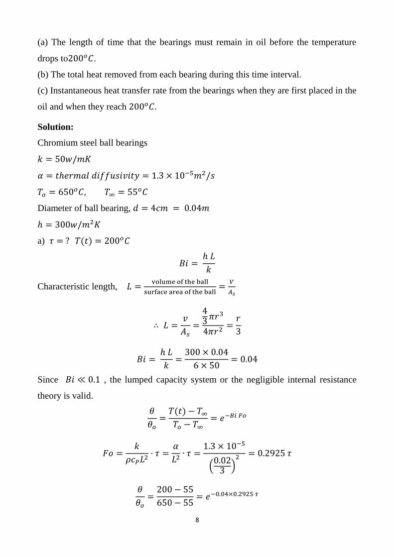
(a) The length of time that the bearings must remain in oil before the temperature

drops to200𝑜𝐶.

(b) The total heat removed from each bearing during this time interval.

(c) Instantaneous heat transfer rate from the bearings when they are first placed in the

oil and when they reach 200𝑜𝐶.

Solution:

Chromium steel ball bearings

𝑘 = 50𝑤/𝑚𝐾

𝛼 = 𝑡ℎ𝑒𝑟𝑚𝑎𝑙 𝑑𝑖𝑓𝑓𝑢𝑠𝑖𝑣𝑖𝑡𝑦 = 1.3 × 10−5𝑚2/𝑠

𝑇𝑜 = 650𝑜𝐶, 𝑇∞ = 55𝑜𝐶

Diameter of ball bearing, 𝑑 = 4𝑐𝑚 = 0.04𝑚

ℎ = 300𝑤/𝑚2𝐾

a) 𝜏 = ? 𝑇(𝑡) = 200𝑜𝐶

𝐵𝑖 = ℎ 𝐿

𝑘

Characteristic length, 𝐿 =volume of the ball

surface area of the ball=

𝑉

𝐴𝑠

∴ 𝐿 =𝑣

𝐴𝑠=

43

𝜋𝑟3

4𝜋𝑟2=

𝑟

3

𝐵𝑖 = ℎ 𝐿

𝑘=

300 × 0.04

6 × 50= 0.04

Since 𝐵𝑖 ≪ 0.1 , the lumped capacity system or the negligible internal resistance

theory is valid.

𝜃

𝜃𝑜=

𝑇(𝑡) − 𝑇∞

𝑇𝑜 − 𝑇∞= 𝑒−𝐵𝑖 𝐹𝑜

𝐹𝑜 =𝑘

𝜌𝑐𝑃𝐿2⋅ 𝜏 =

𝛼

𝐿2∙ 𝜏 =

1.3 × 10−5

(0.02

3 )2 = 0.2925 𝜏

𝜃

𝜃𝑜=

200 − 55

650 − 55= 𝑒−0.04×0.2925 𝜏

9

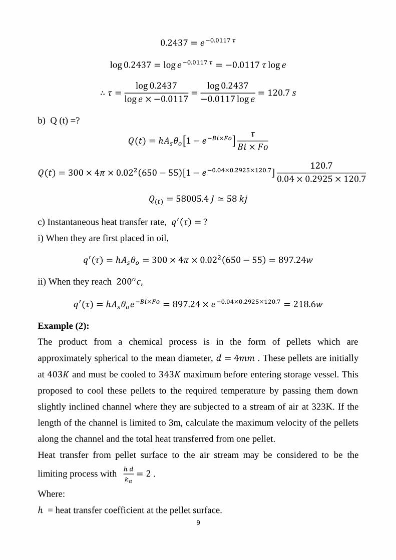
0.2437 = 𝑒−0.0117 𝜏

log 0.2437 = log 𝑒−0.0117 𝜏 = −0.0117 𝜏 log 𝑒

∴ 𝜏 =log 0.2437

log 𝑒 × −0.0117=

log 0.2437

−0.0117 log 𝑒= 120.7 𝑠

b) Q (t) =?

𝑄(𝑡) = ℎ𝐴𝑠𝜃𝑜[1 − 𝑒−𝐵𝑖×𝐹𝑜]𝜏

𝐵𝑖 × 𝐹𝑜

𝑄(𝑡) = 300 × 4𝜋 × 0.022(650 − 55)[1 − 𝑒−0.04×0.2925×120.7]120.7

0.04 × 0.2925 × 120.7

𝑄(𝑡) = 58005.4 𝐽 ≃ 58 𝑘𝑗

c) Instantaneous heat transfer rate, 𝑞′(𝜏) = ?

i) When they are first placed in oil,

𝑞′(𝜏) = ℎ𝐴𝑠𝜃𝑜 = 300 × 4𝜋 × 0.022(650 − 55) = 897.24𝑤

ii) When they reach 200𝑜𝑐,

𝑞′(𝜏) = ℎ𝐴𝑠𝜃𝑜𝑒−𝐵𝑖×𝐹𝑜 = 897.24 × 𝑒−0.04×0.2925×120.7 = 218.6𝑤

Example (2):

The product from a chemical process is in the form of pellets which are

approximately spherical to the mean diameter, 𝑑 = 4𝑚𝑚 . These pellets are initially

at 403𝐾 and must be cooled to 343𝐾 maximum before entering storage vessel. This

proposed to cool these pellets to the required temperature by passing them down

slightly inclined channel where they are subjected to a stream of air at 323K. If the

length of the channel is limited to 3m, calculate the maximum velocity of the pellets

along the channel and the total heat transferred from one pellet.

Heat transfer from pellet surface to the air stream may be considered to be the

limiting process with ℎ 𝑑

𝑘𝑎= 2 .

Where:

ℎ = heat transfer coefficient at the pellet surface.

10

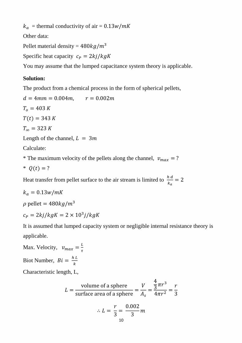
𝑘𝑎 = thermal conductivity of air = 0.13𝑤/𝑚𝐾

Other data:

Pellet material density = 480𝑘𝑔/𝑚3

Specific heat capacity 𝑐𝑃 = 2𝑘𝑗/𝑘𝑔𝐾

You may assume that the lumped capacitance system theory is applicable.

Solution:

The product from a chemical process in the form of spherical pellets,

𝑑 = 4𝑚𝑚 = 0.004𝑚, 𝑟 = 0.002𝑚

𝑇𝑜 = 403 𝐾

𝑇(𝑡) = 343 𝐾

𝑇∞ = 323 𝐾

Length of the channel, 𝐿 = 3𝑚

Calculate:

* The maximum velocity of the pellets along the channel, 𝑣𝑚𝑎𝑥 = ?

* 𝑄(𝑡) = ?

Heat transfer from pellet surface to the air stream is limited to ℎ 𝑑

𝑘𝑎= 2

𝑘𝑎 = 0.13𝑤/𝑚𝐾

𝜌 pellet = 480𝑘𝑔/𝑚3

𝑐𝑃 = 2𝑘𝑗/𝑘𝑔𝐾 = 2 × 103𝑗/𝑘𝑔𝐾

It is assumed that lumped capacity system or negligible internal resistance theory is

applicable.

Max. Velocity, 𝑣𝑚𝑎𝑥 =𝐿

𝜏

Biot Number, 𝐵𝑖 = ℎ 𝐿

𝑘

Characteristic length, L,

𝐿 =volume of a sphere

surface area of a sphere=

𝑉

𝐴𝑠=

43

𝜋𝑟3

4𝜋𝑟2=

𝑟

3

∴ 𝐿 = 𝑟

3=

0.002

3𝑚

11

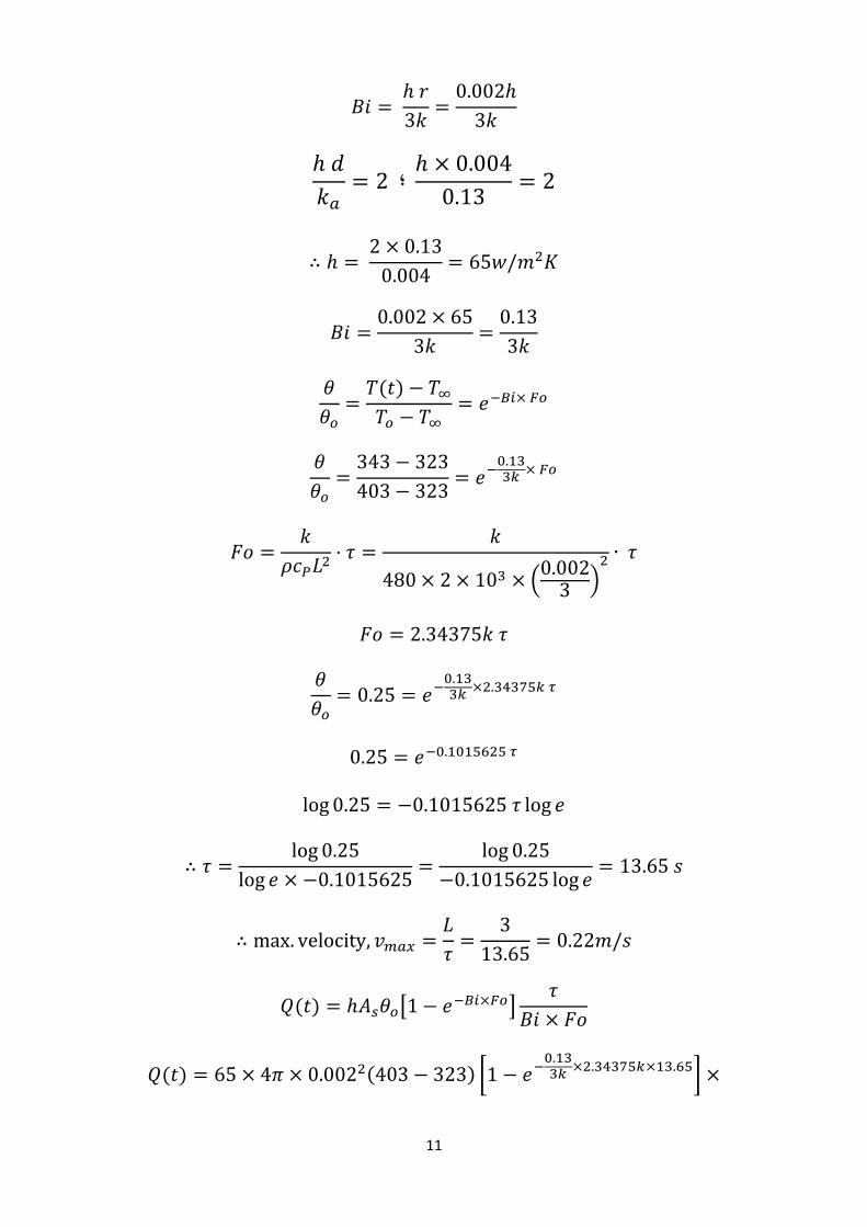
𝐵𝑖 = ℎ 𝑟

3𝑘=

0.002ℎ

3𝑘

ℎ 𝑑

𝑘𝑎= ؛ 2

ℎ × 0.004

0.13= 2

∴ ℎ = 2 × 0.13

0.004= 65𝑤/𝑚2𝐾

𝐵𝑖 =0.002 × 65

3𝑘=

0.13

3𝑘

𝜃

𝜃𝑜=

𝑇(𝑡) − 𝑇∞

𝑇𝑜 − 𝑇∞= 𝑒−𝐵𝑖× 𝐹𝑜

𝜃

𝜃𝑜=

343 − 323

403 − 323= 𝑒−

0.133𝑘

× 𝐹𝑜

𝐹𝑜 =𝑘


𝑘

480 × 2 × 103 × (0.002

3 )2 ∙ 𝜏

𝐹𝑜 = 2.34375𝑘 𝜏

𝜃

𝜃𝑜= 0.25 = 𝑒−

0.133𝑘

×2.34375𝑘 𝜏

0.25 = 𝑒−0.1015625 𝜏

log 0.25 = −0.1015625 𝜏 log 𝑒

∴ 𝜏 =log 0.25

log 𝑒 × −0.1015625=

log 0.25

−0.1015625 log 𝑒= 13.65 𝑠

∴ max. velocity, 𝑣𝑚𝑎𝑥 =𝐿

𝜏=

3

13.65= 0.22𝑚/𝑠



𝑄(𝑡) = 65 × 4𝜋 × 0.0022(403 − 323) [1 − 𝑒−0.133𝑘

×2.34375𝑘×13.65] ×

12

13.65

0.133

× 2.34375 × 13.05= 1.93 𝐽/ pellet

∴ 𝑄(𝑡) = 1.93 𝐽/ pellet

Example (3):

A piece of chromium steel of length 7.4cm (density=8780kg/m3 ; 𝑘 = 50𝑤/𝑚𝐾 and

specific heat 𝑐𝑃 = 440𝑗/𝑘𝑔𝐾) with mass 1.27kg is rolled into a solid cylinder and

heated to a temperature of 600oC and quenched in oil at 36oc. Show that the lumped

capacitance system analysis is applicable and find the temperature of the cylinder

after 4min. What is the total heat transfer during this period?

You may take the convective heat transfer coefficient between the oil and cylinder at

280w/m2k.

Solution:

A piece of chromium steel, L = 7.4cm = 0.074m

𝜌 = 8780𝑘𝑔/𝑚3; 𝑘 = 50𝑤/𝑚𝐾; 𝑐𝑝 = 440𝑗/𝑘𝑔𝐾; 𝑚 = 1.27𝑘𝑔

Rolled into a solid cylinder,

𝑇𝑜 = 600𝑜𝐶; 𝑇∞ = 36𝑜𝐶; ℎ = 280𝑤/𝑚2𝐾

𝑇(𝑡) =? 𝑎𝑓𝑡𝑒𝑟 4𝑚𝑖𝑛 . (𝑖. 𝑒. 𝜏 = 4 × 60 = 240𝑠); 𝑄(𝑡) =?

𝐵𝑖 =ℎ 𝐿

𝑘

Characteristic length, 𝐿 =volume of a cylinder

surface area of a cylinder=

𝑉

𝐴𝑠

=𝜋𝑟2𝐿

2𝜋𝑟𝐿=

𝑟

2

∴ 𝐵𝑖 = ℎ𝑟

2𝑘

𝑉 =𝑚

𝜌=

1.27

8780= 1.4465 × 10−4𝑚3

13

𝐿 = 7.4𝑐𝑚 = 0.074𝑚

𝑉 = 𝜋𝑟2𝐿 = 1.4465 × 10−4

∴ 𝑟 = √1.4465 × 10−4

𝜋 × 0.074= 0.025𝑚

𝐵𝑖 =ℎ 𝑟

2𝑘=

280 × 0.025

2 × 50= 0.07

Since 𝐵𝑖 ≪ 0.1 , then the system is assumed to be of lumped capacitance system,

and therefore the lumped capacitance system analysis or the negligible internal

resistance theory is applicable.

𝑇(𝑡) =?

𝜏 = 4 × 60 = 240 𝑠

𝜃

𝜃𝑜=

𝑇(𝑡) − 𝑇∞

𝑇𝑜 − 𝑇∞= 𝑒−𝐵𝑖 𝐹𝑜

𝐹𝑜 =𝑘

𝜌𝑐𝑃𝐿2⋅ 𝜏

𝐹𝑜 =50

8780 × 440 × (0.025

2 )2 × 240 = 19.88

𝜃

𝜃𝑜=

𝑇(𝑡) − 36

600 − 36= 𝑒−0.07×19.88

𝑇(𝑡) − 36

564= 𝑒−1.3916

∴ 𝑇(𝑡) = 56 + 𝑒−1.3916 + 36 = 176. 254𝑜𝐶

𝑞′(𝜏)=0 = 𝑞′(0) = ℎ𝐴𝑠𝜃𝑜 = ℎ𝐴𝑠(𝑇𝑜 − 𝑇∞)

= 280 × 2𝜋 × 0.025 × 0.074(600 − 36) = 1835.65𝑤

𝑞′(𝜏)=4𝑚𝑖𝑛 = ℎ𝐴𝑠𝜃𝑜𝑒−𝐵𝑖 ×𝐹𝑜

14

= 1835.65 × 𝑒−1.3916 = 456.5𝑤

Total heat transfer rate,

𝑄(𝑡) = ℎ𝐴𝑠𝜃𝑜(1 − 𝑒−𝐵𝑖 ×𝐹𝑜)𝜏


𝑄(𝑡) = 1835.65(1 − 𝑒−1.3916)240

1.3916= 237855.57 J

≃ 237.86 𝑘𝑗

Example (4):

A piece of aluminum (𝜌 = 2705𝑘𝑔/𝑚3, 𝑘 = 216𝑤/𝑚𝐾, 𝑐𝑃 = 896𝑗/𝑘𝑔𝐾) having a

mass of 4.78kg and initially at temperature of 290𝑜𝐶 is suddenly immersed in a fluid

at 15𝑜𝐶.

The convection heat transfer coefficient is 54𝑤/𝑚2𝐾 . Taking the aluminum as a

sphere having the same mass as that given, estimate the time required to cool the

aluminum to 90𝑜𝐶.

Find also the total heat transferred during this period. (Justify your use of the lumped

capacity method of analysis).

Solution:

A piece of aluminum

𝜌 = 2705𝑘𝑔/𝑚3; 𝑘 = 216𝑤/𝑚𝐾; 𝑐𝑝 = 896𝐽/𝑘𝑔𝐾; 𝑚 = 4.78𝑘𝑔

𝑇𝑜 = 290𝑜𝐶;

𝑇∞ = 15𝑜𝐶;

ℎ = 24𝑤/𝑚2𝐾;

Taking aluminum as a sphere.

Estimate 𝜏 = ? 𝑇(𝑡) = 90𝑜𝐶 ; 𝑄(𝑡) =?

𝜃

𝜃𝑜=

𝑇(𝑡) − 𝑇∞

𝑇𝑜 − 𝑇∞= 𝑒−𝐵𝑖 ×𝐹𝑜

𝐵𝑖 =ℎ 𝐿

𝑘

15

The characteristic length, 𝐿 =𝑉

𝐴𝑠=

4

3𝜋𝑟3

4𝜋𝑟2=

𝑟

3

∴ 𝐵𝑖 = ℎ 𝑟

3𝑘

𝜌 =𝑚

𝑉 ; 𝑉 =

𝑚

𝜌=

4.78

2705=

4

3𝜋𝑟3

𝑟 = √4.78

2705×

3

4𝜋

3

= 0.075𝑚

∴ 𝐵𝑖 =54 × 0.075

3 × 216= 0.00625

If 𝐵𝑖 ≪ 0.1 , then the system is assumed to be of lumped capacity.

Since 𝐵𝑖 = 0.00625 ≪ 0.1 , therefore the lumped capacity method of analysis is

used.

𝐹𝑜 =𝑘


216

2705 × 896 × (0.075

3 )2 ∙ 𝜏

𝐹𝑜 = 0.1426 𝜏

𝜃

𝜃𝑜=

90 − 15

290 − 15= 𝑒−0.00625×0.1426 𝜏

75

275= 𝑒−8.9125×10−4 𝜏

log75

275= −8.9125 × 10−4 𝜏 log 𝑒

∴ 𝜏 =log

75275

−8.9125 × 10−4 𝜏 log 𝑒= 1457.8 𝑠

Total heat transfer rate, Q(t),



16

𝑄(𝑡) = 54 × 4𝜋 × 0.0752(290 − 15)[1 − 𝑒−8.9125×10−4 ×1457.8] ×

1457.8

8.9125 × 10−4 × 1457.8= 856552 𝐽 = 856.6 𝑘𝑗

∴ 𝑄(𝑡) = 856552 𝐽 = 856.6 𝑘𝑗

17

Chapter Two

Time Constant and Response of Temperature Measuring

Instruments

2.1 Introduction:

Measurement of temperature by a thermocouple is an important application of

the lumped parameter analysis. The response of a thermocouple is defined as the time

required for the thermocouple to attain the source temperature.

It is evident from equation (1.4), that the larger the quantity ℎ𝐴𝑠

𝜌𝑉𝑐𝑃 , the faster the

exponential term will approach zero or the more rapid will be the response of the

temperature measuring device. This can be accomplished either by increasing the

value of "h" or by decreasing the wire diameter, density and specific heat. Hence, a

very thin wire is recommended for use in thermocouples to ensure a rapid response

(especially when the thermocouples are employed for measuring transient

temperatures).

From equation (1.8);


𝜏=

ℎ𝐴𝑠

𝜌𝑉𝑐𝑃

𝜌𝑉𝑐𝑃

ℎ𝐴𝑠=

𝜏


The quantity 𝜌𝑉𝑐𝑃

ℎ𝐴𝑠 (which has units of time) is called time constant and is denoted by

the symbol 𝜏∗ . Thus,

𝜏

𝐵𝑖 × 𝐹𝑜= 𝜏∗ =

𝜌𝑉𝑐𝑃

ℎ𝐴𝑠=

𝑘

𝛼ℎ∙

𝑉

𝐴𝑠 (2.1)

{Since 𝛼 = 𝑘

𝜌𝑐𝑝}

And,

18

𝜃

𝜃𝑜=

𝑇(𝑡) − 𝑇∞

𝑇𝑜 − 𝑇∞= 𝑒−𝐵𝑖×𝐹𝑜 = 𝑒−(𝜏/𝜏∗) (2.2)

At 𝜏 = 𝜏∗ (one time constant), we have from equation (2.2),

𝜃

𝜃𝑜=

𝑇(𝑡) − 𝑇∞

𝑇𝑜 − 𝑇∞= 𝑒−1 = 0.368 (2.3)

Thus, 𝜏∗ is the time required for the temperature change to reach 36.8% of its final

value in response to a step change in temperature. In other words, temperature

difference would be reduced by 63.2%. The time required by a thermocouple to

reach its 63.2% of the value of initial temperature difference is called its sensitivity.

Depending upon the type of fluid used the response times for different sizes of

thermocouple wires usually vary between 0.04 to 2.5 seconds.


Example (1):

A thermocouple junction of spherical form is to be used to measure the temperature

of a gas stream.

ℎ = 400𝑤/𝑚2𝑜𝐶; 𝑘(thermocouple junction) = 20𝑤/𝑚𝑜𝐶; 𝑐𝑝 = 400𝐽/𝑘𝑔𝑜𝐶;

and 𝜌 = 8500𝑘𝑔/𝑚3;

Calculate the following:

(i) Junction diameter needed for the thermocouple to have thermal time constant of

one second.

(ii) Time required for the thermocouple junction to reach 198𝑜𝑐 if junction is initially

at 25𝑜𝐶 and is placed in gas stream which is at 200𝑜𝐶 .

Solution:

Given: ℎ = 400𝑤/𝑚2𝑜𝐶; 𝑘(thermocouple junction) = 20𝑤/𝑚𝑜𝐶;

𝑐𝑝 = 400𝐽/𝑘𝑔𝑜𝐶; 𝜌 =8500𝑘𝑔

𝑚3.

(i) Junction diameter, d =?

𝜏∗ (thermal time constant) = 1 s

19

The time constant is given by:

𝜏∗ =𝜌𝑉𝑐𝑃

ℎ𝐴𝑠=

𝜌 ×43

𝜋𝑟3 × 𝑐𝑃

ℎ × 4𝜋𝑟2=

𝜌𝑟𝑐𝑃

3ℎ

or 1 =8500 × 𝑟 × 400

3 × 400

∴ 𝑟 = 3

8500= 3.53 × 10−4𝑚 = 0.353𝑚𝑚

∴ 𝑑 = 2𝑟 = 2 × 0.353 = 0.706𝑚𝑚

(ii) Time required for the thermocouple junction to reach 198𝑜𝐶; 𝜏 =?

Given: 𝑇𝑜 = 25𝑜𝐶; 𝑇∞ = 200𝑜𝐶; 𝑇(𝑡) = 198𝑜𝐶;

𝐵𝑖 =ℎ 𝐿𝑐

𝑘

𝐿𝑐 of a sphere = 𝑟

3

∴ 𝐵𝑖 =ℎ(𝑟/3)

𝑘=

400 × (0.353 × 10−3/3)

20= 0.00235

As Bi is much less than 0.1, the lumped capacitance method can be used. Now,

𝑇(𝑡) − 𝑇∞

𝑇𝑜 − 𝑇∞= 𝑒−𝐵𝑖×𝐹𝑜 = 𝑒−(𝜏/𝜏∗)

𝐹𝑜 =𝑘


20

8500 × 400 × (0.353 × 10−3

3 )2 ∙ 𝜏 = 424.86 𝜏

𝐵𝑖 × 𝐹𝑜 = 0.00235 × 424.86 𝜏 = 0.998𝜏

∴ 𝐵𝑖 × 𝐹𝑜 =𝜏

𝜏∗= 0.998𝜏

∵ 𝜏∗ = 1 , therefore, 𝜏 = 0.998𝜏

∴𝜃

𝜃𝑜=

198 − 200

25 − 200= 𝑒−0.998𝜏

20

0.01143 = 𝑒−0.998𝜏

−0.998𝜏 ln 𝑒 = ln 0.01143

∴ 𝜏 =ln 0.01143

−0.998 × 1= 4.48 𝑠

Example (2):

A thermocouple junction is in the form of 8mm diameter sphere. Properties of

material are:

𝑐𝑝 = 420𝐽/𝑘𝑔𝑜𝐶; 𝜌 = 8000𝑘𝑔/𝑚3; 𝑘 = 40𝑤/𝑚𝑜𝐶; ℎ = 40𝑤/𝑚2𝑜𝐶;

This junction is initially at 40𝑜𝐶 and inserted in a stream of hot air at 300𝑜𝐶 . Find

the following:

(i) Time constant of the thermocouple.

(ii) The thermocouple is taken out from the hot air after 10 seconds and kept in still

air at 30𝑜𝐶. Assuming the heat transfer coefficient in air 𝑖𝑠 10𝑤/𝑚2𝑜𝐶, find the

temperature attained by the junction 20 seconds after removal from hot air.

Solution:

Given: 𝑟 =8

2= 4𝑚𝑚 = 0.004𝑚; 𝑐𝑝 =

420𝐽

𝑘𝑔𝑜𝑐; 𝜌 =

8000𝑘𝑔

𝑚3; 𝑘 = 40𝑤/𝑚𝑜𝐶

ℎ = 40𝑤/𝑚2𝑜𝐶 (gas stream or hot air); ℎ = 10𝑤/𝑚2𝑜

𝐶 (still air)

(i) Time constant of the thermocouple, 𝜏∗ =?

𝜏∗ =𝜏

𝐵𝑖 × 𝐹𝑜=

𝜌𝑉𝑐𝑃

ℎ𝐴𝑠=

𝜌 ×43

𝜋𝑟3 × 𝑐𝑃

ℎ × 4𝜋𝑟2=

𝜌𝑟𝑐𝑃

3ℎ

∴ 𝜏∗ =8000 × 0.004 × 420

3 × 40= 112 𝑠 (when thermocouple is in gas stream)

(ii) The temperature attained by the junction, ; 𝑇(𝑡) =?

Given: 𝑇𝑜 = 40𝑜𝐶; 𝑇∞ = 300𝑜𝐶; 𝜏 = 10 𝑠;

The temperature variation with respect to time during heating (when dipped in gas

stream) is given by:

21

𝜃

𝜃𝑜=

𝑇(𝑡) − 𝑇∞

𝑇𝑜 − 𝑇∞= 𝑒−𝐵𝑖×𝐹𝑜 = 𝑒−(𝜏/𝜏∗)

𝑜𝑟 𝑇(𝑡) − 300

40 − 300= 𝑒−(𝜏/𝜏∗) = 𝑒−(10/112) = 0.9146

∴ 𝑇(𝑡) = −260 × 0.9146 + 300 = 62.2𝑜𝐶

The temperature variation with respect to time during cooling (when exposed to air)

is given by:

𝑇(𝑡) − 𝑇∞

𝑇𝑜 − 𝑇∞= 𝑒−(𝜏/𝜏∗)

where 𝜏∗ =𝜌𝑟𝑐𝑃

3ℎ=

8000 × 0.004 × 420

3 × 10= 448 𝑠

∴ 𝑇(𝑡) − 30

62.2 − 30= 𝑒(−20/448) = 0.9563

𝑜𝑟 𝑇(𝑇) = (62.2 − 30) × 0.9563 + 30 = 60.79𝑜𝐶

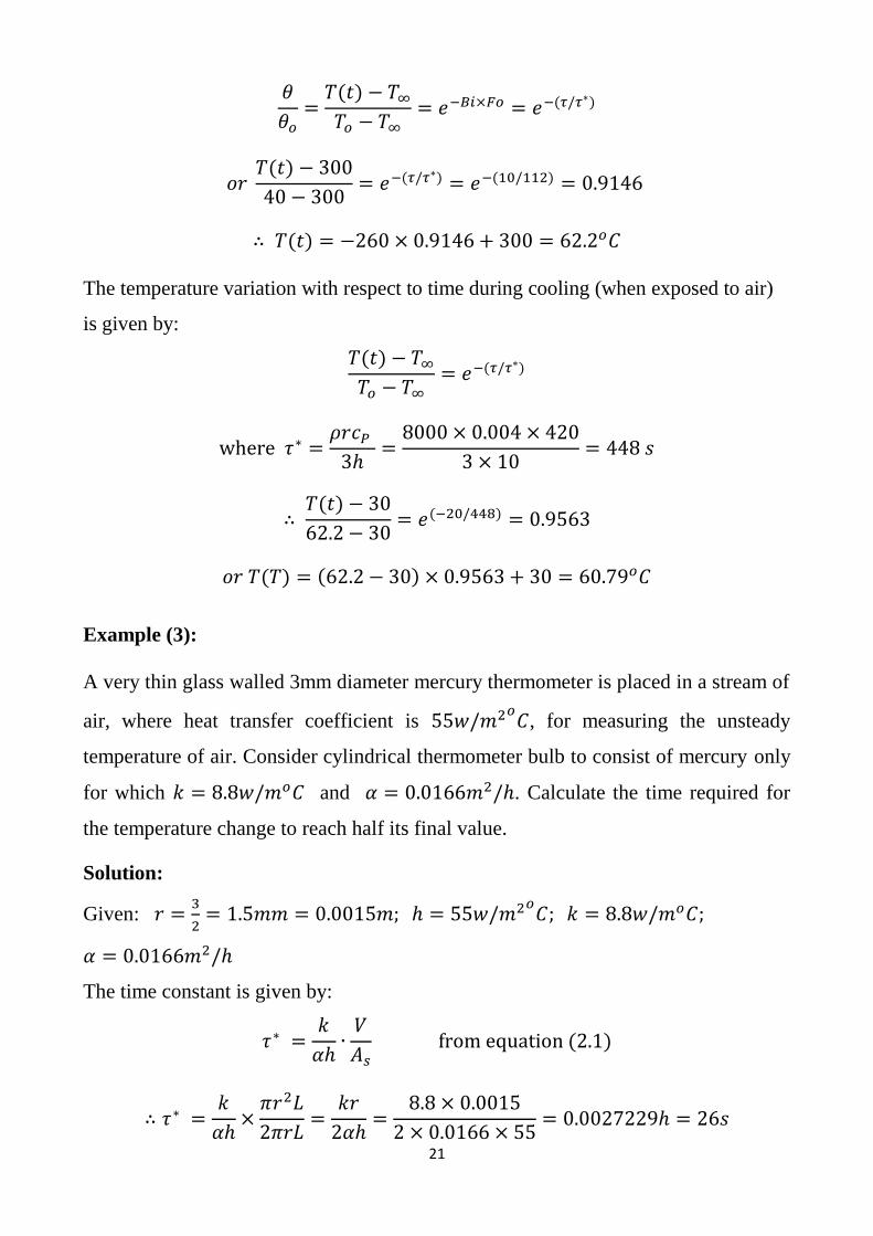
Example (3):

A very thin glass walled 3mm diameter mercury thermometer is placed in a stream of

air, where heat transfer coefficient is 55𝑤/𝑚2𝑜𝐶, for measuring the unsteady

temperature of air. Consider cylindrical thermometer bulb to consist of mercury only

for which 𝑘 = 8.8𝑤/𝑚𝑜𝐶 and 𝛼 = 0.0166𝑚2/ℎ. Calculate the time required for

the temperature change to reach half its final value.

Solution:

Given: 𝑟 =3

2= 1.5𝑚𝑚 = 0.0015𝑚; ℎ = 55𝑤/𝑚2𝑜

𝐶; 𝑘 = 8.8𝑤/𝑚𝑜𝐶;

𝛼 = 0.0166𝑚2/ℎ

The time constant is given by:

𝜏∗ =𝑘

𝛼ℎ∙

𝑉

𝐴𝑠 from equation (2.1)

∴ 𝜏∗ =𝑘

𝛼ℎ×

𝜋𝑟2𝐿

2𝜋𝑟𝐿=

𝑘𝑟

2𝛼ℎ=

8.8 × 0.0015

2 × 0.0166 × 55= 0.0027229ℎ = 26𝑠

22

For temperature change to reach half its final value

𝜃

𝜃𝑜=

1

2= 𝑒−(𝜏/𝜏∗)

ln1

2= ln 𝑒−𝜏/𝜏∗

ln1

2= −𝜏/𝜏∗ ln 𝑒

−𝜏

𝜏∗=

ln12

ln 𝑒= ln

1

2= −0.693

∴𝜏

𝜏∗= 0.693

𝑜𝑟 𝜏 = 𝜏∗ × 0.693 = 26 × 0.693 = 18.02 𝑠

Note: Thus, one can expect thermometer to record the temperature trend accurately

only for unsteady temperature changes which are slower.

Example (4):

The temperature of an air stream flowing with a velocity of 3m/s is measured by a

copper – constantan thermocouple which may be approximately as a sphere of 2.5mm

in diameter. Initially the junction and air are at a temperature of 25𝑜𝐶. The air

temperature suddenly changes to and is maintained at 215𝑜𝐶.

(i) Determine the time required for the thermocouple to indicate a temperature of

165𝑜𝐶. Also, determine the thermal time constant and the temperature indicated by

the thermocouple at that instant.

(ii) Discuss the stability of this thermocouple to measure unsteady state temperature

of a fluid when the temperature variation in the fluid has a time period of 3.6s.

The thermal junction properties are:

𝜌 = 8750𝑘𝑔/𝑚3; 𝑐𝑝 = 380𝐽/𝑘𝑔𝑜𝐶; 𝑘(thermocouple) = 28𝑤/𝑚𝑜𝐶; 𝑎𝑛𝑑

ℎ = 145𝑤/𝑚2𝑜𝐶;

Solution:

23

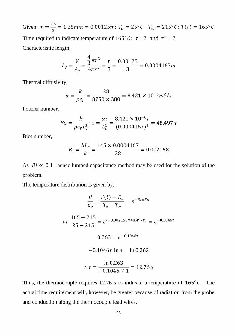
Given: 𝑟 =2.5

2= 1.25𝑚𝑚 = 0.00125𝑚; 𝑇𝑜 = 25𝑜𝐶; 𝑇∞ = 215𝑜𝐶; 𝑇(𝑡) = 165𝑜𝐶

Time required to indicate temperature of 165𝑜𝐶; 𝜏 =? and 𝜏∗ = ?;

Characteristic length,

𝐿𝑐 =𝑉

𝐴𝑠=

43

𝜋𝑟3

4𝜋𝑟2=

𝑟

3=

0.00125

3= 0.0004167𝑚

Thermal diffusivity,

𝛼 =𝑘

𝜌𝑐𝑃=

28

8750 × 380= 8.421 × 10−6𝑚2/𝑠

Fourier number,

𝐹𝑜 =𝑘

𝜌𝑐𝑃𝐿𝑐2

∙ 𝜏 =𝛼𝜏

𝐿𝑐2

=8.421 × 10−6𝜏

(0.0004167)2= 48.497 𝜏

Biot number,

𝐵𝑖 =ℎ𝐿𝑐

𝑘=

145 × 0.0004167

28= 0.002158

As 𝐵𝑖 ≪ 0.1 , hence lumped capacitance method may be used for the solution of the

problem.

The temperature distribution is given by:

𝜃

𝜃𝑜=

𝑇(𝑡) − 𝑇∞

𝑇𝑜 − 𝑇∞= 𝑒−𝐵𝑖×𝐹𝑜

𝑜𝑟 165 − 215

25 − 215= 𝑒(−0.002158×48.497𝜏) = 𝑒−0.1046𝜏

0.263 = 𝑒−0.1046𝜏

−0.1046𝜏 ln 𝑒 = ln 0.263

∴ 𝜏 =ln 0.263

−0.1046 × 1= 12.76 𝑠

Thus, the thermocouple requires 12.76 s to indicate a temperature of 165𝑜𝐶 . The

actual time requirement will, however, be greater because of radiation from the probe

and conduction along the thermocouple lead wires.

24

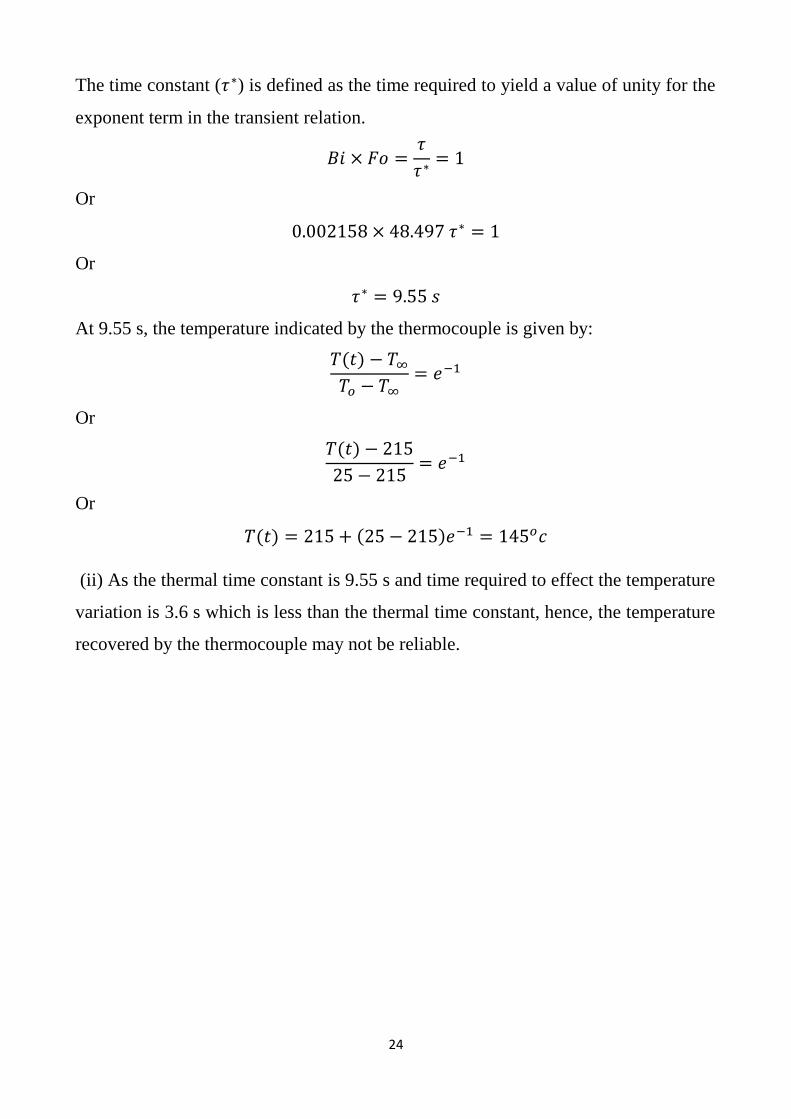
The time constant (𝜏∗) is defined as the time required to yield a value of unity for the

exponent term in the transient relation.

𝐵𝑖 × 𝐹𝑜 =𝜏

𝜏∗= 1

Or

0.002158 × 48.497 𝜏∗ = 1

Or

𝜏∗ = 9.55 𝑠

At 9.55 s, the temperature indicated by the thermocouple is given by:

𝑇(𝑡) − 𝑇∞

𝑇𝑜 − 𝑇∞= 𝑒−1

Or

𝑇(𝑡) − 215

25 − 215= 𝑒−1

Or

𝑇(𝑡) = 215 + (25 − 215)𝑒−1 = 145𝑜𝑐

(ii) As the thermal time constant is 9.55 s and time required to effect the temperature

variation is 3.6 s which is less than the thermal time constant, hence, the temperature

recovered by the thermocouple may not be reliable.

25

Chapter Three

Transient Heat Conduction in Solids with Finite Conduction

and Convective Resistances [𝟎 < 𝑩𝒊 < 𝟏𝟎𝟎]

3.1 Introduction:

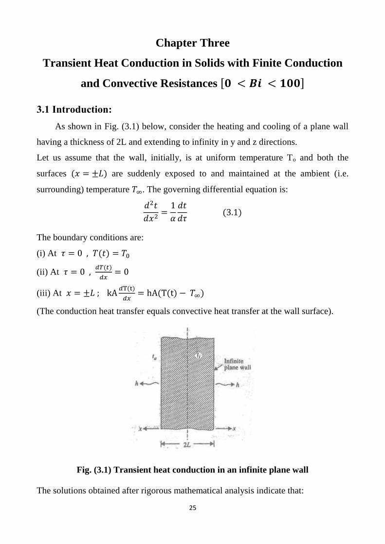
As shown in Fig. (3.1) below, consider the heating and cooling of a plane wall

having a thickness of 2L and extending to infinity in y and z directions.

Let us assume that the wall, initially, is at uniform temperature To and both the

surfaces (𝑥 = ±𝐿) are suddenly exposed to and maintained at the ambient (i.e.

surrounding) temperature 𝑇∞. The governing differential equation is:

𝑑2𝑡

𝑑𝑥2=

1

𝛼

𝑑𝑡

𝑑𝜏 (3.1)

The boundary conditions are:

(i) At 𝜏 = 0 , 𝑇(𝑡) = 𝑇0

(ii) At 𝜏 = 0 ,𝑑𝑇(𝑡)

𝑑𝑥= 0

(iii) At 𝑥 = ±𝐿 ; kA𝑑T(t)

𝑑𝑥= hA(T(t) − 𝑇∞)

(The conduction heat transfer equals convective heat transfer at the wall surface).

Fig. (3.1) Transient heat conduction in an infinite plane wall

The solutions obtained after rigorous mathematical analysis indicate that:

26

𝑇(𝑡) − 𝑇∞

𝑇𝑜 − 𝑇∞= 𝑓 [

𝑥

𝐿,ℎ𝑙

𝑘,𝛼𝜏

𝑙2] (3.2)

From equation (3.2), it is evident that when conduction resistance is not negligible,

the temperature history becomes a function of Biot numbers {ℎ𝑙

𝑘}, Fourier number

{𝛼𝜏

𝑙2 } and the dimensionless parameter {𝑥

𝐿} which indicates the location of point within

the plate where temperature is to be obtained. The dimensionless parameter {𝑥

𝐿} is

replaced by {𝑟

𝑅} in case of cylinders and spheres.

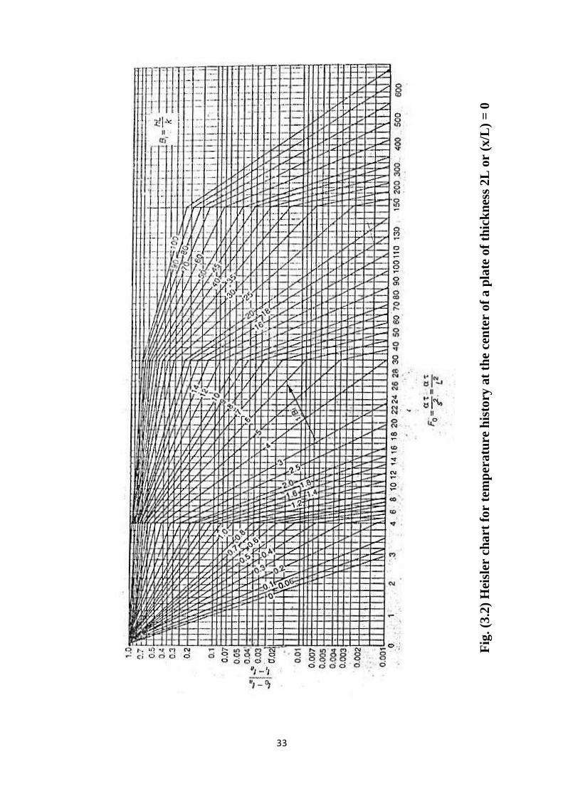
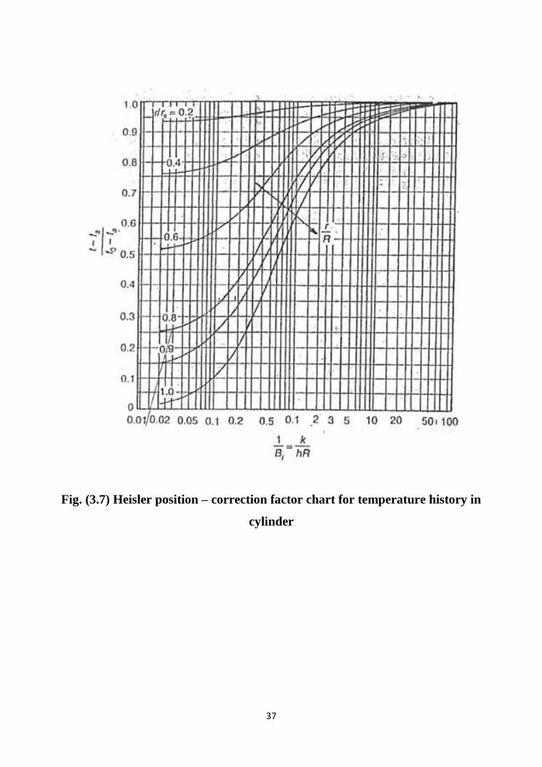
For the equation (3.2) graphical charts have been prepared in a variety of forms. In

the Figs. from (3.2) to (3.4) the Heisler charts are shown which depict the

dimensionless temperature [𝑇𝑐−𝑇∞

𝑇𝑜−𝑇∞] versus Fo (Fourier number) for various values of

(1

𝐵𝑖) for solids of different geometrical shapes such as plates, cylinders and spheres.

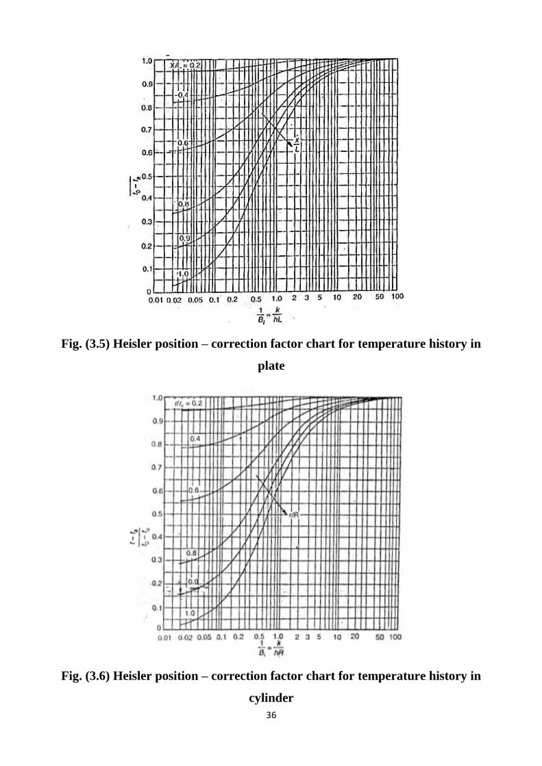
These charts provide the temperature history of the solid at its mid – plane (𝑥 = 0)

and the temperatures at other locations are worked out by multiplying the mid – plane

temperature by correction factors read from charts given in figs. (3.5) to (3.7). The

following relationship is used:

𝜃

𝜃𝑜=

𝑇(𝑡) − 𝑇∞

𝑇𝑜 − 𝑇∞= [

𝑇𝑐 − 𝑇∞

𝑇𝑜 − 𝑇∞] × [

𝑇(𝑡) − 𝑇∞

𝑇𝑐 − 𝑇∞]

The values 𝐵𝑖 (Biot number) and 𝐹𝑜 (Fourier number), as used in Heisler charts, are

evaluated on the basis of a characteristic parameter 𝑠 which is the semi – thickness in

the case of plates and the surface radius in case of cylinders and spheres.

When both conduction and convection resistances are almost of equal importance the

Heister charts are extensively used to determine the temperature distribution.


Example (1):

A 60 mm thickness large steel plate (𝑘 = 42.6𝑤/𝑚𝑜𝐶, 𝛼 = 0.043𝑚2/ℎ), initially at

440𝑜𝐶 is suddenly exposed on both sides to an environment with convective heat

transfer coefficient 235𝑤/𝑚2𝑜𝐶, and temperature 50𝑜𝐶. Determine the center line

27

temperature, and temperature inside the plate 15𝑚𝑚 from the mid – plane after 4.3

minutes.

Solution:

Given: 2𝐿 = 60𝑚𝑚 = 0.06𝑚, 𝑘 = 42.6𝑤/𝑚𝑜𝐶, 𝛼 = 0.043𝑚2/ℎ, 𝑇𝑜 = 440𝑜𝐶,

ℎ = 235𝑤/𝑚2𝑜𝐶, 𝑇∞ = 50𝑜𝐶, 𝜃 = 4.3𝑚𝑖𝑛𝑢𝑡𝑒𝑠.

Temperature at the mid – plane (centerline) of the plate 𝑇𝑐:

The characteristic length, 𝐿𝑐 =60

2= 30𝑚𝑚 = 0.03𝑚

Fourier number, 𝐹𝑜 =𝛼𝜏

𝐿𝑐2 =

0.043×(4.3/60)

(0.03)2= 3.424

Biot number, 𝐵𝑖 =ℎ𝐿𝑐

𝑘=

235×0.03

42.6= 0.165

At 𝐵𝑖 > 0.1, the internal temperature gradients are not small, therefore, internal

resistance cannot be neglected. Thus, the plate cannot be considered as a lumped

system. Further, as the 𝐵𝑖 < 100, Heisler charts can be used to find the solution of

the problem.

Corresponding to the following parametric values, from Heisler charts Fig. (3.2), we

have 𝐹𝑜 = 3.424; 1

𝐵𝑖=

1

0.165= 6.06 and

𝑥

𝐿= 0 (mid – plane).


𝑇𝑜 − 𝑇∞= 0.6 [from Heisler charts]

Substituting the values, we have

𝑇𝑐 − 50

440 − 50= 0.6

Or

𝑇𝑐 = 50 + 0.6(440 − 50) = 248𝑜𝐶

Temperature inside the plate 15mm from the mid - plane, 𝑇(𝑡) =? the distance 15mm

from the mid – plane implies that:

𝑥

𝐿=

15

30= 0.5

Corresponding to 𝑥

𝐿= 0.5 and

1

𝐵𝑖= 6.06, from Fig. (3.5), we have:

28

𝑇(𝑡) − 𝑇∞

𝑇𝑐 − 𝑇∞= 0.97

Substituting the values, we get:

𝑇(𝑡) − 50

284 − 50= 0.97

Or

𝑇(𝑡) = 50 + 0.97(284 − 50) = 276.98𝑜𝐶

Example (2):

A 6 mm thick stainless steel plate (𝜌 = 7800𝑘𝑔/𝑚3, 𝑐𝑝 = 460𝐽/𝑘𝑔𝑜𝐶, 𝑘 =

55𝑤/𝑚𝑜𝐶) is used to form the nose section of a missile. It is held initially at a

uniform temperature of 30𝑜𝐶. When the missile enters the denser layers of the

atmosphere at a very high velocity the effective temperature of air surrounding the

nose region attains 2150𝑜𝐶; the surface convective heat transfer coefficient is

estimated 3395𝑤/𝑚2𝑜𝐶. If the maximum metal temperature is not to exceed

1100𝑜𝐶, determine:

(i) Maximum permissible time in these surroundings.

(ii) Inside surface temperature under these conditions.

Solution:

Given: 2𝐿 = 6𝑚𝑚 = 0.006𝑚, 𝑘 = 55𝑤/𝑚𝑜𝐶, 𝑐𝑝 = 460𝐽/𝑘𝑔𝑜 𝐶, 𝑇𝑜 = 30𝑜𝐶,

𝜌 = 7800𝑘𝑔/𝑚3, 𝑇∞ = 2150𝑜𝐶, 𝑇(𝑡) = 1100𝑜𝐶

(i) Maximum permissible time, 𝜏 = ?

Characteristic length, 𝐿𝑐 =0.006

2= 0.003𝑚

Biot number, 𝐵𝑖 =ℎ𝐿

𝑘=

3395×0.003

55= 0.185

As 𝐵𝑖 > 0.1, therefore, lumped analysis cannot be applied in this case. Further, as

𝐵𝑖 < 100, Heisler charts can be used to obtain the solution of the problem.

Corresponding to 1

𝐵𝑖= 5.4 and

𝑥

𝐿= 1 (outside surface of nose section, from Fig.

(3.5), we have),

29

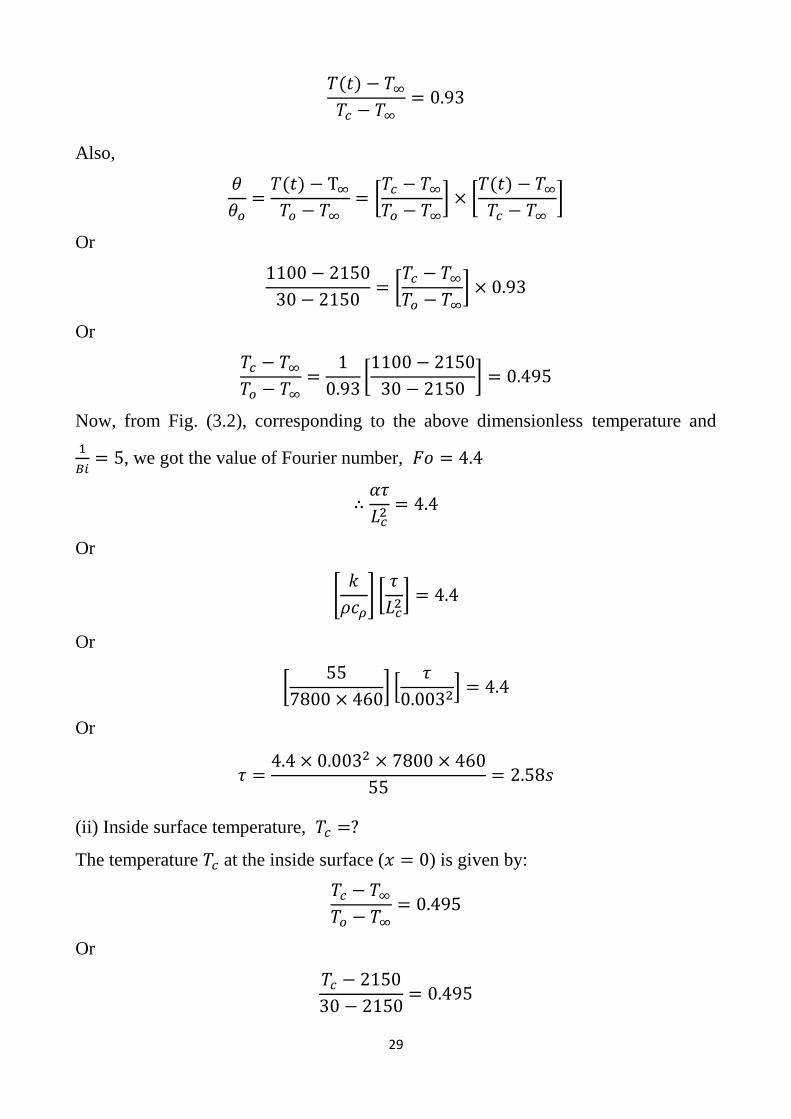
𝑇(𝑡) − 𝑇∞

𝑇𝑐 − 𝑇∞= 0.93

Also,

𝜃

𝜃𝑜=

𝑇(𝑡) − T∞

𝑇𝑜 − 𝑇∞= [


𝑇𝑜 − 𝑇∞] × [

𝑇(𝑡) − 𝑇∞

𝑇𝑐 − 𝑇∞]

Or

1100 − 2150

30 − 2150= [


𝑇𝑜 − 𝑇∞] × 0.93

Or


𝑇𝑜 − 𝑇∞=

1

0.93[1100 − 2150

30 − 2150] = 0.495

Now, from Fig. (3.2), corresponding to the above dimensionless temperature and

1

𝐵𝑖= 5, we got the value of Fourier number, 𝐹𝑜 = 4.4

∴𝛼𝜏

𝐿𝑐2

= 4.4

Or

[𝑘

𝜌𝑐𝜌] [

𝜏

𝐿𝑐2

] = 4.4

Or

[55

7800 × 460] [

𝜏

0.0032] = 4.4

Or

𝜏 =4.4 × 0.0032 × 7800 × 460

55= 2.58𝑠

(ii) Inside surface temperature, 𝑇𝑐 =?

The temperature 𝑇𝑐 at the inside surface (𝑥 = 0) is given by:


𝑇𝑜 − 𝑇∞= 0.495

Or

𝑇𝑐 − 2150

30 − 2150= 0.495

30

Or

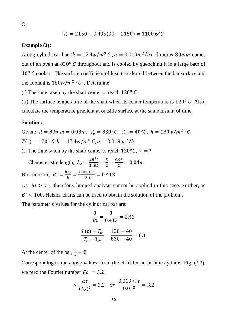
𝑇𝑐 = 2150 + 0.495(30 − 2150) = 1100.6𝑜𝐶

Example (3):

Along cylindrical bar (𝑘 = 17.4𝑤/𝑚𝑜 𝐶 , 𝛼 = 0.019𝑚2/ℎ) of radius 80𝑚𝑚 comes

out of an oven at 830𝑜 𝐶 throughout and is cooled by quenching it in a large bath of

40𝑜 𝐶 coolant. The surface coefficient of heat transferred between the bar surface and

the coolant is 180𝑤/𝑚2 𝑜𝐶 . Determine:

(i) The time taken by the shaft center to reach 120𝑜 𝐶 .

(ii) The surface temperature of the shaft when its center temperature is 120𝑜 𝐶. Also,

calculate the temperature gradient at outside surface at the same instant of time.

Solution:

Given: 𝑅 = 80𝑚𝑚 = 0.08𝑚, 𝑇𝑜 = 830𝑜𝐶, 𝑇∞ = 40𝑜𝐶, ℎ = 180𝑤/𝑚2 𝑜𝐶,

𝑇(𝑡) = 120𝑜 𝐶, 𝑘 = 17.4𝑤/𝑚𝑜 𝐶, 𝛼 = 0.019 𝑚2/ℎ.

(i) The time taken by the shaft center to reach 120𝑜𝐶, 𝜏 = ?

Characteristic length, 𝐿𝑐 =𝜋𝑅2𝐿

2𝜋𝑅𝐿=

𝑅

2=

0.08

2= 0.04𝑚


𝑘=

180×0.04

17.4= 0.413

As 𝐵𝑖 > 0.1, therefore, lumped analysis cannot be applied in this case. Further, as

𝐵𝑖 < 100, Heisler charts can be used to obtain the solution of the problem.

The parametric values for the cylindrical bar are:

1

𝐵𝑖=

1

0.413= 2.42

𝑇(𝑡) − 𝑇∞

𝑇𝑜 − 𝑇∞=

120 − 40

830 − 40= 0.1

At the center of the bar, 𝑟

𝑅= 0

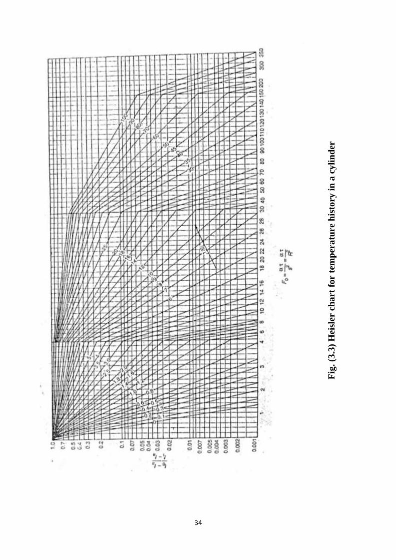
Corresponding to the above values, from the chart for an infinite cylinder Fig. (3.3),

we read the Fourier number 𝐹𝑜 = 3.2 .

∴ 𝛼𝜏

(𝐿𝑐)2= 3.2 𝑜𝑟

0.019 × 𝜏

0.042= 3.2

31

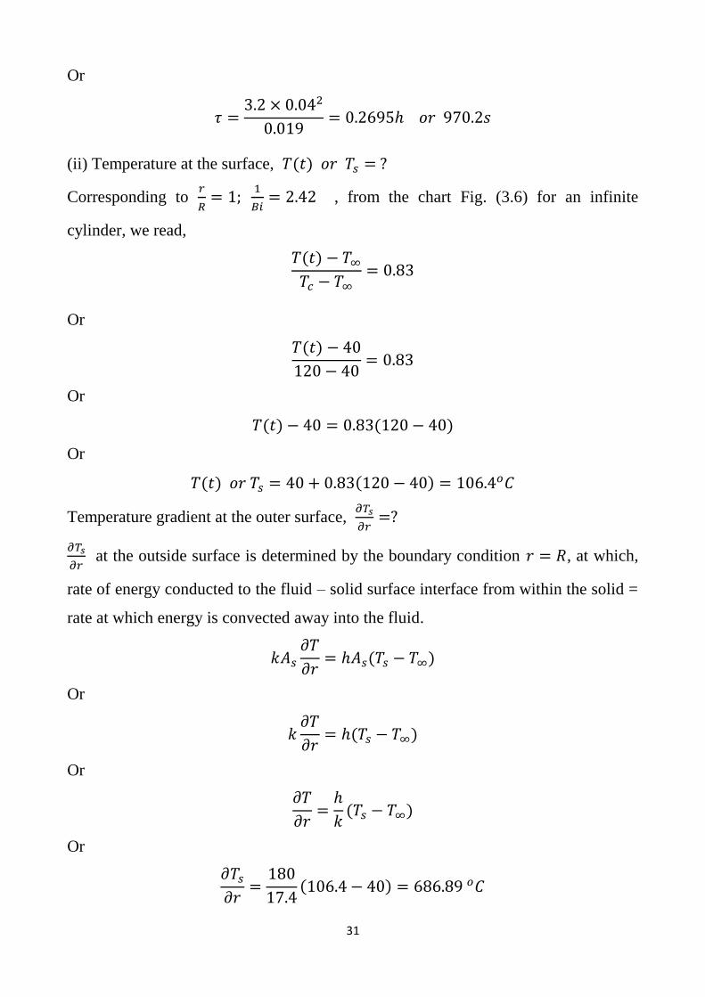
Or

𝜏 =3.2 × 0.042

0.019= 0.2695ℎ 𝑜𝑟 970.2𝑠

(ii) Temperature at the surface, 𝑇(𝑡) 𝑜𝑟 𝑇𝑠 = ?

Corresponding to 𝑟

𝑅= 1;

1

𝐵𝑖= 2.42 , from the chart Fig. (3.6) for an infinite

cylinder, we read,

𝑇(𝑡) − 𝑇∞

𝑇𝑐 − 𝑇∞= 0.83

Or

𝑇(𝑡) − 40

120 − 40= 0.83

Or

𝑇(𝑡) − 40 = 0.83(120 − 40)

Or

𝑇(𝑡) 𝑜𝑟 𝑇𝑠 = 40 + 0.83(120 − 40) = 106.4𝑜𝐶

Temperature gradient at the outer surface, 𝜕𝑇𝑠

𝜕𝑟=?

𝜕𝑇𝑠

𝜕𝑟 at the outside surface is determined by the boundary condition 𝑟 = 𝑅, at which,

rate of energy conducted to the fluid – solid surface interface from within the solid =

rate at which energy is convected away into the fluid.

𝑘𝐴𝑠

𝜕𝑇

𝜕𝑟= ℎ𝐴𝑠(𝑇𝑠 − 𝑇∞)

Or

𝑘𝜕𝑇

𝜕𝑟= ℎ(𝑇𝑠 − 𝑇∞)

Or

𝜕𝑇

𝜕𝑟=

ℎ

𝑘(𝑇𝑠 − 𝑇∞)

Or

𝜕𝑇𝑠

𝜕𝑟=

180

17.4(106.4 − 40) = 686.89 𝑜𝐶

32

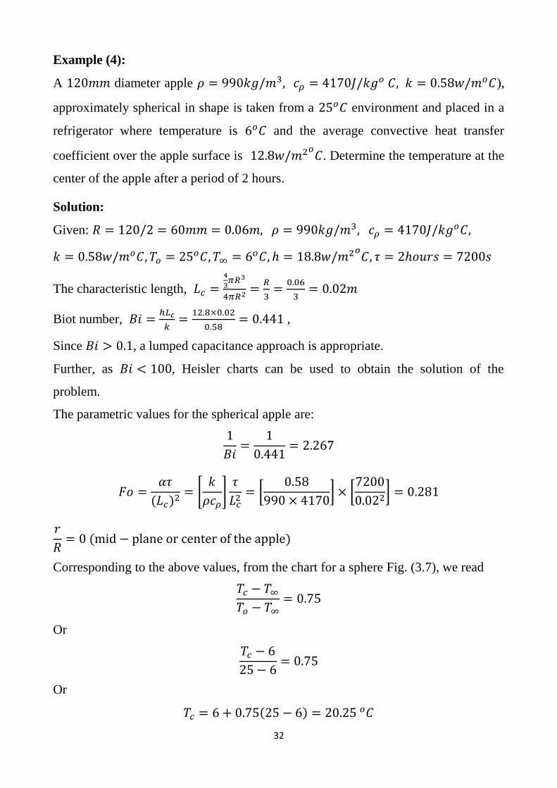
Example (4):

A 120𝑚𝑚 diameter apple 𝜌 = 990𝑘𝑔/𝑚3, 𝑐𝜌 = 4170𝐽/𝑘𝑔𝑜 𝐶, 𝑘 = 0.58𝑤/𝑚𝑜𝐶),

approximately spherical in shape is taken from a 25𝑜𝐶 environment and placed in a

refrigerator where temperature is 6𝑜𝐶 and the average convective heat transfer

coefficient over the apple surface is 12.8𝑤/𝑚2𝑜𝐶. Determine the temperature at the

center of the apple after a period of 2 hours.

Solution:

Given: 𝑅 = 120/2 = 60𝑚𝑚 = 0.06𝑚, 𝜌 = 990𝑘𝑔/𝑚3, 𝑐𝜌 = 4170𝐽/𝑘𝑔𝑜𝐶,

𝑘 = 0.58𝑤/𝑚𝑜𝐶, 𝑇𝑜 = 25𝑜𝐶, 𝑇∞ = 6𝑜𝐶, ℎ = 18.8𝑤/𝑚2𝑜𝐶, 𝜏 = 2ℎ𝑜𝑢𝑟𝑠 = 7200𝑠

The characteristic length, 𝐿𝑐 =4

3𝜋𝑅3

4𝜋𝑅2=

𝑅

3=

0.06

3= 0.02𝑚


𝑘=

12.8×0.02

0.58= 0.441 ,

Since 𝐵𝑖 > 0.1, a lumped capacitance approach is appropriate.

Further, as 𝐵𝑖 < 100, Heisler charts can be used to obtain the solution of the

problem.

The parametric values for the spherical apple are:

1

𝐵𝑖=

1

0.441= 2.267

𝐹𝑜 =𝛼𝜏

(𝐿𝑐)2= [

𝑘

𝜌𝑐𝜌]

𝜏

𝐿𝑐2

= [0.58

990 × 4170] × [

7200

0.022] = 0.281

𝑟

𝑅= 0 (mid − plane or center of the apple)

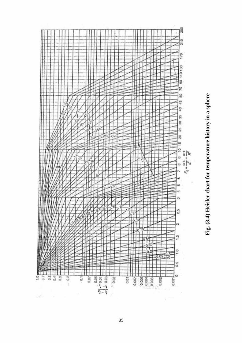
Corresponding to the above values, from the chart for a sphere Fig. (3.7), we read


𝑇𝑜 − 𝑇∞= 0.75

Or

𝑇𝑐 − 6

25 − 6= 0.75

Or

𝑇𝑐 = 6 + 0.75(25 − 6) = 20.25 𝑜𝐶

33

Fig

. (3

.2)

Hei

sler

ch

art

fo

r te

mp

era

ture

his

tory

at

the

cen

ter

of

a p

late

of

thic

kn

ess

2L

or

(x/L

) =

0

34

Fig

. (3

.3)

Hei

sler

ch

art

fo

r te

mp

era

ture

his

tory

in

a c

yli

nd

er

35

Fig

. (3

.4)

Hei

sler

ch

art

fo

r te

mp

era

ture

his

tory

in

a s

ph

ere

36

Fig. (3.5) Heisler position – correction factor chart for temperature history in

plate


cylinder

37


cylinder

38

Chapter Four

Transient Heat conduction in semi – infinite solids

[𝑯 𝒐𝒓 𝑩𝒊 → ∞] 4.1 Introduction:

A solid which extends itself infinitely in all directions of space is termed as an

infinite solid. If an infinite solid is split in the middle by a plane, each half is known

as semi – infinite solid. In a semi – infinite body, at any instant of time, there is

always a point where the effect of heating (or cooling) at one of its boundaries is not

felt at all. At the point the temperature remains unaltered. The transient temperature

change in a plane of infinitely thick wall is similar to that of a semi – infinite body

until enough time has passed for the surface temperature effect to penetrate through

it.

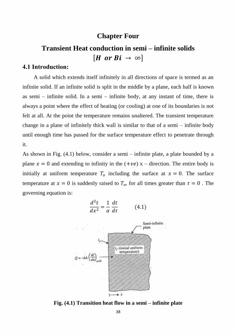
As shown in Fig. (4.1) below, consider a semi – infinite plate, a plate bounded by a

plane 𝑥 = 0 and extending to infinity in the (+𝑣𝑒) x – direction. The entire body is

initially at uniform temperature 𝑇𝑜 including the surface at 𝑥 = 0. The surface

temperature at 𝑥 = 0 is suddenly raised to 𝑇∞ for all times greater than 𝜏 = 0 . The

governing equation is:

𝑑2𝑡

𝑑𝑥2=

1

𝛼 𝑑𝑡

𝑑𝜏 (4.1)

Fig. (4.1) Transition heat flow in a semi – infinite plate

39

The boundary conditions are:

(i) 𝑇(𝑥, 0) = 𝑇𝑜 ;

(ii) 𝑇(0, 𝜏) = 𝑇∞ 𝑓𝑜𝑟 𝜏 > 0 ;

(iii) 𝑇(∞, 𝜏) = 𝑇𝑜 𝑓𝑜𝑟 𝜏 > 0 ;

The solution of the above differential equation, with these boundary conditions, for

temperature distribution at any time 𝜏 at a plane parallel to and at a distance 𝑥 from

the surface is given by:

𝑇(𝑥, 𝜏) − 𝑇∞

𝑇𝑜 − 𝑇∞= erf (𝑧) = 𝑒𝑟𝑓 [

𝑥

2√𝛼𝜏] (4.2)

Where 𝑧 =𝑥

2√𝛼𝜏 is known as Gaussian error function and is defined by:

𝑒𝑟𝑓 [𝑥

2√𝛼𝜏] = erf(𝑧) =

2

√𝜋∫ 𝑒−𝜂2

𝑑𝜂 (4.3)𝑧

0

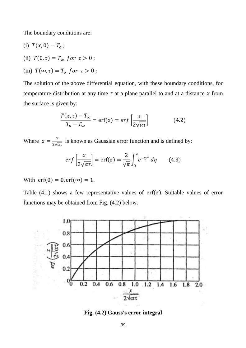
With erf(0) = 0, erf (∞) = 1.

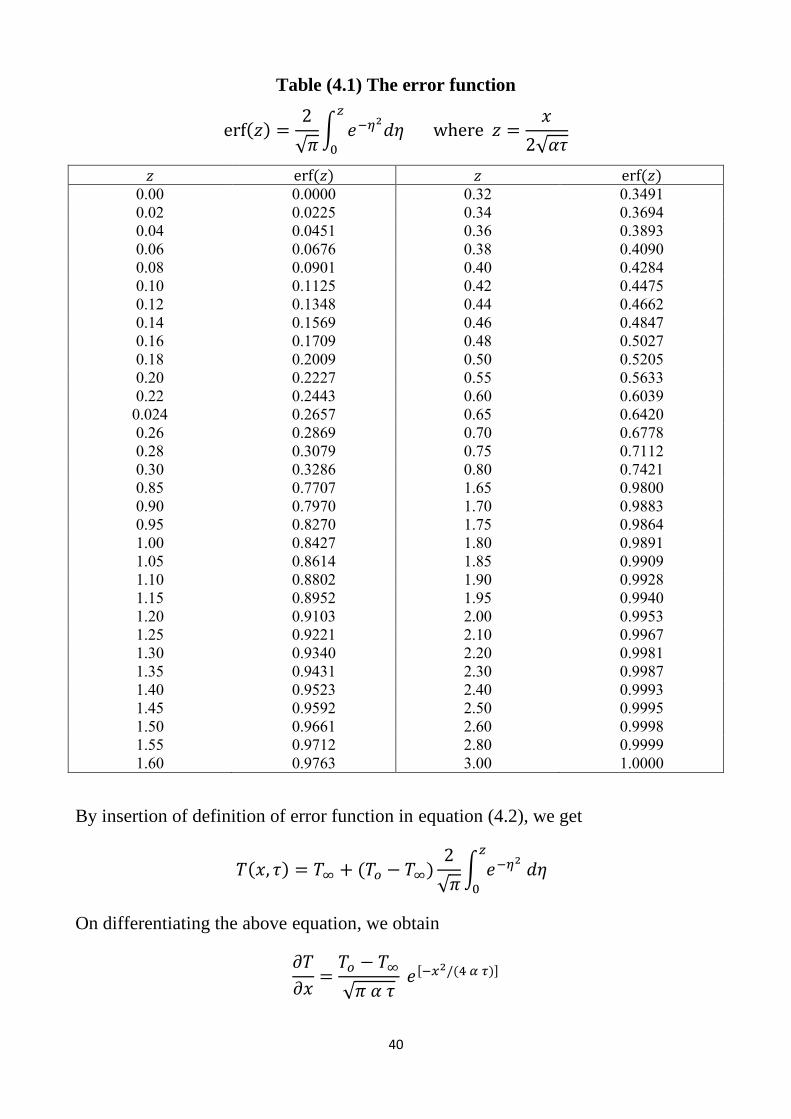
Table (4.1) shows a few representative values of erf(𝑧). Suitable values of error

functions may be obtained from Fig. (4.2) below.

Fig. (4.2) Gauss's error integral

40

Table (4.1) The error function

erf(𝑧) =2

√𝜋∫ 𝑒−𝜂2

𝑑𝜂 where 𝑧 =𝑥

2√𝛼𝜏

𝑧

0

𝑧 erf (𝑧) 𝑧 erf (𝑧)

0.00 0.0000 0.32 0.3491

0.02 0.0225 0.34 0.3694

0.04 0.0451 0.36 0.3893

0.06 0.0676 0.38 0.4090

0.08 0.0901 0.40 0.4284

0.10 0.1125 0.42 0.4475

0.12 0.1348 0.44 0.4662

0.14 0.1569 0.46 0.4847

0.16 0.1709 0.48 0.5027

0.18 0.2009 0.50 0.5205

0.20 0.2227 0.55 0.5633

0.22 0.2443 0.60 0.6039

0.024 0.2657 0.65 0.6420

0.26 0.2869 0.70 0.6778

0.28 0.3079 0.75 0.7112

0.30 0.3286 0.80 0.7421

0.85 0.7707 1.65 0.9800

0.90 0.7970 1.70 0.9883

0.95 0.8270 1.75 0.9864

1.00 0.8427 1.80 0.9891

1.05 0.8614 1.85 0.9909

1.10 0.8802 1.90 0.9928

1.15 0.8952 1.95 0.9940

1.20 0.9103 2.00 0.9953

1.25 0.9221 2.10 0.9967

1.30 0.9340 2.20 0.9981

1.35 0.9431 2.30 0.9987

1.40 0.9523 2.40 0.9993

1.45 0.9592 2.50 0.9995

1.50 0.9661 2.60 0.9998

1.55 0.9712 2.80 0.9999

1.60 0.9763 3.00 1.0000

By insertion of definition of error function in equation (4.2), we get

𝑇(𝑥, 𝜏) = 𝑇∞ + (𝑇𝑜 − 𝑇∞)2

√𝜋∫ 𝑒−𝜂2

𝑑𝜂 𝑧

0

On differentiating the above equation, we obtain

𝜕𝑇

𝜕𝑥=

𝑇𝑜 − 𝑇∞

√𝜋 𝛼 𝜏 𝑒[−𝑥2/(4 𝛼 𝜏)]

41

The instantaneous heat flow rate at a given x – location within the semi – infinite

body at a specified time is given by:

𝑄𝑖𝑛𝑠𝑡𝑎𝑛𝑡𝑎𝑛𝑒𝑜𝑢𝑠 = −𝑘𝐴(𝑇𝑜 − 𝑇∞)𝑒

[−𝑥2

4 𝛼 𝜏]

√𝜋 𝛼 𝜏 (4.4)

By substituting the gradient [𝜕𝑇

𝜕𝑥] in Fourier's law.

The heat flow rate at the surface (𝑥 = 0) is given by:

𝑄𝑠𝑢𝑟𝑓𝑎𝑐𝑒 =−𝑘𝐴(𝑇𝑜 − 𝑇∞)

√𝜋 𝛼 𝜏 (4.5)

The total heat flow rate,

𝑄(𝑡) =−𝑘𝐴(𝑇𝑜 − 𝑇∞)

√𝜋 𝛼 ∫

1

√𝜋𝑑𝜏 = −𝑘𝐴(𝑇𝑜 − 𝑇∞)2√

𝜏

𝜋𝛼

𝜏

0

Or

𝑄(𝑡) = −1.13𝑘𝐴(𝑇𝑜 − 𝑇∞)√𝜏

𝛼 (4.6)

The general criterion for the infinite solution to apply to a body of finite thickness

(slab) subjected to one dimensional heat transfer is:

𝐿

2√𝛼 𝜏 ≥ 0.5

Where, L = thickness of the body.

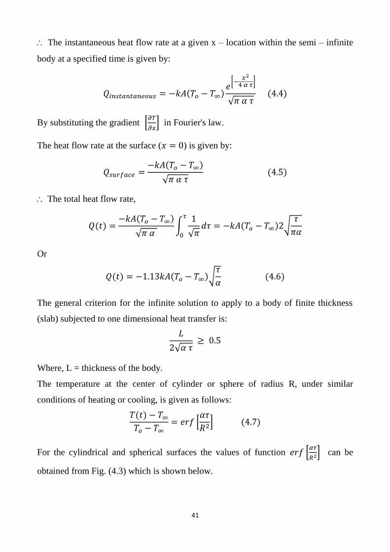
The temperature at the center of cylinder or sphere of radius R, under similar

conditions of heating or cooling, is given as follows:

𝑇(𝑡) − 𝑇∞

𝑇𝑜 − 𝑇∞= 𝑒𝑟𝑓 [

𝛼𝜏

𝑅2] (4.7)

For the cylindrical and spherical surfaces the values of function 𝑒𝑟𝑓 [𝛼𝜏

𝑅2] can be

obtained from Fig. (4.3) which is shown below.

42

Fig. (4.3) Error integral for cylinders and spheres

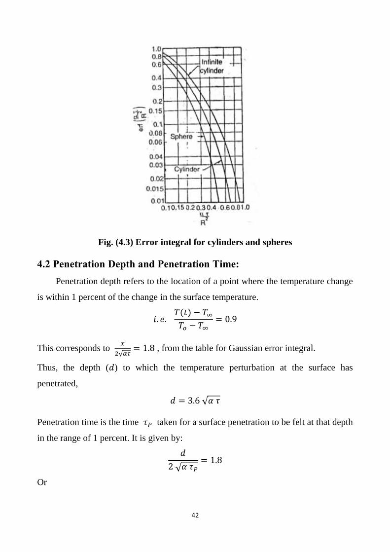
4.2 Penetration Depth and Penetration Time:

Penetration depth refers to the location of a point where the temperature change

is within 1 percent of the change in the surface temperature.

𝑖. 𝑒. 𝑇(𝑡) − 𝑇∞

𝑇𝑜 − 𝑇∞= 0.9

This corresponds to 𝑥

2√𝛼𝜏= 1.8 , from the table for Gaussian error integral.

Thus, the depth (𝑑) to which the temperature perturbation at the surface has

penetrated,

𝑑 = 3.6 √𝛼 𝜏

Penetration time is the time 𝜏𝑃 taken for a surface penetration to be felt at that depth

in the range of 1 percent. It is given by:

𝑑

2 √𝛼 𝜏𝑃

= 1.8

Or

43

𝜏𝑃 =𝑑2

13 𝛼 (4.8)


Example (1):

A steel ingot (large in size) heated uniformly to 745𝑜 𝐶 is hardened by quenching it

in an oil path maintained at 20𝑜 𝐶. Determine the length of time required for the

temperature to reach 595𝑜 𝐶 at a depth of 12𝑚𝑚. The ingot may be approximated as

a flat plate. For steel ingot take 𝛼(thermal diffusivity) = 1.2 × 10−5𝑚2/𝑠

Solution:

Given: 𝑇𝑜 = 745𝑜𝑐, 𝑇∞ = 20𝑜𝑐, 𝑇(𝑡) = 595𝑜𝑐, 𝑥 = 12𝑚𝑚 = 0.012𝑚,

𝛼 = 1.2 × 10−5𝑚2/𝑠, time required, 𝜏 =?

The temperature distribution at any time 𝜏 at a plane parallel to and at a distance 𝑥

from the surface is given by:

𝑇(𝑡) − 𝑇∞

𝑇𝑐 − 𝑇∞= 𝑒𝑟𝑓 [

𝑥

2 √𝛼 𝜏] (4.2)

Or

595 − 20

745 − 20= 0.79 = 𝑒𝑟𝑓 [

𝑥

2 √𝛼 𝜏]

Or

∴ 𝑥

2 √𝛼 𝜏= 0.9 from Table (4.1) or Fig. (4.3)

Or

𝑥2

4 𝛼 𝜏= 0.81

Or

𝜏 =𝑥2

4 𝛼 × 0.81=

0.0122

4 × 1.2 × 10−5 × 0.81= 3.7𝑠

Example (2):

It is proposed to bury water pipes underground in wet soil which is initially at 5.4𝑜 𝐶.

The temperature of the surface of soil suddenly drops to −6𝑜 𝐶 and remains at this

44

value for 9.5 hours. Determine the maximum depth at which the pipes be laid if the

surrounding soil temperature is to remain above 0𝑜 𝐶 (without water getting frozen).

Assume the soil as semi – infinite solid.

For wet soil take 𝛼(thermal diffusivity) = 2.75 × 10−3𝑚2/ℎ

Solution:

Given: 𝑇𝑜 = 5.4𝑜𝐶, 𝑇∞ = −6𝑜𝑐, 𝑇(𝑡) = 0𝑜𝐶, 𝛼 = 2.75 × 10−3𝑚2/𝑠, maximum

depth 𝑥 =?

The temperature, at critical depth, will just reach after 9.5 hours,

Now,

𝑇(𝑡) − 𝑇∞


𝑥

2 √𝛼 𝜏] (4.2)

Or

0 − (−6)

5.4 − (−6)= 0.526 = 𝑒𝑟𝑓 [

𝑥

√2 𝛼 𝜏]

Or

𝑥

2 √𝛼 𝜏≃ 0.5 from Table (4.1)or Fig. (4.3)

Or

𝑥 = 0.5 × 2 √𝛼 𝜏

Or

𝑥 = 0.5 × 2 √2.75 × 10−3 × 9.5 = 0.162𝑚

Example (3):

A 60𝑚𝑚 thick mild steel plate (𝛼 = 1.22 × 10−5𝑚2/𝑠) is initially at a temperature

of 30𝑜 𝐶. It is suddenly exposed on one side to a fluid which causes the surface

temperature to increase to and remain at 110𝑜 𝐶 . Determine:

(i) The maximum time that the slab be treated as a semi – infinite body;

(ii) The temperature at the center of the slab 1.5 minutes after the change in surface

temperature.

45

Solution:

Given: 𝐿 = 60𝑚𝑚 = 0.06𝑚, 𝛼 = 1.22 × 10−5𝑚2/𝑠, 𝑇𝑜 = 30𝑜𝐶, 𝑇∞ = 110𝑜𝐶,

𝜏 = 1.5 𝑚𝑖𝑛𝑢𝑡𝑒𝑠 = 90 𝑠

(i) The maximum time that the slab be treated as a semi – infinite body, (𝜏𝑚𝑎𝑥 = ).

The general criterion for the infinite solution to apply to a body of finite thickness

subjected to one – dimensional heat transfer is:

𝐿

2 √𝛼 𝜏≥ 0.5 (where L = thickness of the body)

Or

𝐿

2 √𝛼 𝜏𝑚𝑎𝑥

= 0.5 or 𝐿2

4 𝛼 𝜏𝑚𝑎𝑥= 0.25

Or

𝜏𝑚𝑎𝑥 =𝐿2

4 𝛼 × 0.25=

0.062

4 × 1.22 × 10−5 × 0.25= 295.1 𝑠

(ii) The temperature at the center of the slab, 𝑇(𝑡) =?

At the center of the slab, 𝑥 = 0.03𝑚 ; 𝜏 = 90 𝑠

𝑇(𝑡) − 𝑇∞


𝑥

2 √𝛼 𝜏]

Or

𝑇(𝑡) = 𝑇∞ + 𝑒𝑟𝑓 [𝑥

2 √𝛼 𝜏] (𝑇𝑜 − 𝑇∞)

Where:

𝑒𝑟𝑓 [𝑥

2 √𝛼 𝜏] = 𝑒𝑟𝑓 [

0.03

2 √1.22 × 10−5 × 90] = erf(0.453)

≃ 0.47 [from Table (4.1)]

𝑇(𝑡) = 𝑇𝑐 = 110 + 0.47(30 − 110) = 72.4𝑜𝐶

Example (4):

The initial uniform temperature of a thick concrete wall (𝛼 = 1.6 × 10−3𝑚2/ℎ, 𝑘 =

0.9𝑤/𝑚𝑜𝐶) of a jet engine test cell is 25𝑜𝐶. The surface temperature of the wall

46

suddenly rises to 340𝑜𝐶 when the combination of exhaust gases from the turbo jet …

spray of cooling water occurs. Determine:

(i) The temperature at a point 80mm from the surface after 8 hours.

(ii) The instantaneous heat flow rate at the specified plane and at the surface itself at

the instant mentioned at (i).

Use the solution for semi – infinite solid.

Solution:

Given: 𝑇𝑜 = 25𝑜𝐶, 𝑇∞ = 340𝑜𝐶, 𝛼 = 1.6 × 10−3𝑚2/ℎ, 𝑘 = 0.94𝑤/𝑚𝑜𝐶, 𝜏 = 8ℎ,

𝑥 = 80𝑚𝑚 = 0.08𝑚

(i) The temperature at a point 0.08m from the surface; 𝑇(𝑡) =?

𝑇(𝑡) − 𝑇∞


𝑥

2 √𝛼 𝜏]

Or

𝑇(𝑡) = 𝑇∞ + 𝑒𝑟𝑓 [𝑥

2 √𝛼 𝜏] (𝑇𝑜 − 𝑇∞)

Where

𝑒𝑟𝑓 [𝑥

2 √𝛼 𝜏] = 𝑒𝑟𝑓 [

0.03

2 √1.6 × 10−3 × 8] = erf(0.353) ≃ 0.37

∴ 𝑇(𝑡) = 340 + 0.37(25 − 340) = 223.45𝑜𝐶

(ii) The instantaneous heat flow rate, 𝑄𝑖𝑛𝑠𝑡𝑎𝑛𝑡𝑎𝑛𝑒𝑜𝑢𝑠 at the specified plane =?

𝑄𝑖 = −𝑘𝐴(𝑇𝑜 − 𝑇∞)𝑒

[−𝑥2

4 𝛼 𝜏]

√𝜋 𝛼 𝜏 from equation (4.4)

𝑄𝑖 = −0.94 × 1 × (25 − 340)𝑒[−0.082/(4×1.6×10−3×8)]

√𝜋 × 1.6 × 10−3 × 8

= −296.1 ×0.8825

0.2005= −1303.28𝑤/𝑚2 of wall area

The negative sign shows the heat lost from the wall.

Heat flow rate at the surface itself, 𝑄𝑠𝑢𝑟𝑓𝑎𝑐𝑒 =?

47

𝑄𝑠𝑢𝑟𝑓𝑎𝑐𝑒 𝑜𝑟 𝑄𝑠 = −𝑘𝐴(𝑇𝑜 − 𝑇∞)

√𝜋 𝛼 𝜏 from equation(4.5)

= −0.94 × 1 × (25 − 340)

√𝜋 × 1.6 × 10−3 × 8 = (−)1476.6𝑤 per 𝑚2 of wall area

Example (5):

The initial uniform temperature of a large mass of material (𝛼 = 0.42𝑚2/ℎ) is

120𝑜𝐶. The surface is suddenly exposed to and held permanently at 6𝑜𝐶. Calculate

the time required for the temperature gradient at the surface to reach 400𝑜𝐶/𝑚.

Solution:

Given: 𝑇𝑜 = 120𝑜𝐶, 𝑇∞ = 6𝑜𝐶, 𝛼 = 0.42𝑚2/ℎ,

[𝜕 𝑇

𝜕 𝑥]

𝑥=0 (temperature gradient at the surface) = 400𝑜𝐶/𝑚

Time required, 𝜏 =?

Heat flow rate at the surface (𝑥 = 0) is given by:

𝑄𝑠𝑢𝑟𝑓𝑎𝑐𝑒 = −𝑘𝐴(𝑇𝑜 − 𝑇∞)

√𝜋 𝛼 𝜏 from equation (4.5)

Or

−𝑘𝐴 [𝜕 𝑇

𝜕 𝑥]

𝑥=0 = −

𝑘𝐴(𝑇𝑜 − 𝑇∞)

√𝜋 𝛼 𝜏

Or

[𝜕 𝑇

𝜕 𝑥]

𝑥=0 =

𝑇𝑜 − 𝑇∞

√𝜋 𝛼 𝜏

substituting the values above, we obtain:

400 =(120 − 6)

√𝜋 × 0.42 × 𝜏

Or

𝜋 × 0.42𝜏 = [120 − 6

400]

2

= 0.0812

Or

48

𝜏 =0.0812

𝜋 × 0.42= 0.0615ℎ = 221.4 𝑠

Example (6):

A motor car of mass 1600kg travelling at 90km/h, is brought to reset within a period

of 9 seconds when the brakes are applied. The braking system consists of 4 brakes

with each brake band of 360 cm2 area, these press against steel drums of equivalent

area. The brake lining and the drum surface (𝑘 = 54𝑤/𝑚𝑜𝐶, 𝛼 = 1.25 × 10−5𝑚2/𝑠)

are at the same temperature and the heat generated during the stoppage action

dissipates by flowing across drums. The drum surface is treated as semi – infinite

plane, calculate the maximum temperature rise.

Solution:

Given: 𝑚 = 1600𝑘𝑔, 𝑣(velocity) = 90𝑘𝑚/ℎ, 𝜏 = 9𝑠, 𝐴(Area of 4 brake bands)

= 4 × 360 × 10−4𝑚2 𝑜𝑟 0.144𝑚2, 𝑘 = 54𝑤/𝑚𝑜𝐶, 𝛼 = 1.25 × 10−5𝑚2/𝑠.

Maximum temperature rise, 𝑇∞ − 𝑇𝑜 =?

When the car comes to rest (after applying brakes), its kinetic energy is converted

into heat energy which is dissipated through the drums.

Kinetic energy of the moving car = 1

2𝑚𝑣2

=1

2× 1600 × [

90 × 1000

60 × 60]

2

= 5 × 105J in 9 seconds

∴ Heat flow rate = 5 × 105

9= 0.555 × 105J /s 𝑜𝑟 𝑤

This value equals the instantaneous heat flow rate at the surface (𝑥 = 0), which is

given by:

(𝑄𝑖)𝑠𝑢𝑟𝑓𝑎𝑐𝑒 = −𝑘𝐴(𝑇𝑜 − 𝑇∞)

√𝜋 𝛼 𝜏= 0.555 × 105 from equation (4.5)

Or

−54 × 0.144(𝑇𝑜 − 𝑇∞)

√𝜋 × 1.25 × 10−5 × 9= 0.555 × 105

49

Or

−(𝑇𝑜 − 𝑇∞) =0.555 × 105 × √𝜋 × 1.25 × 10−5 × 9

54 × 0.144= 134.3

Or

𝑇𝑜 − 𝑇∞ = 134.3𝑜𝐶

Hence, maximum temperature rise = 134.3𝑜𝐶

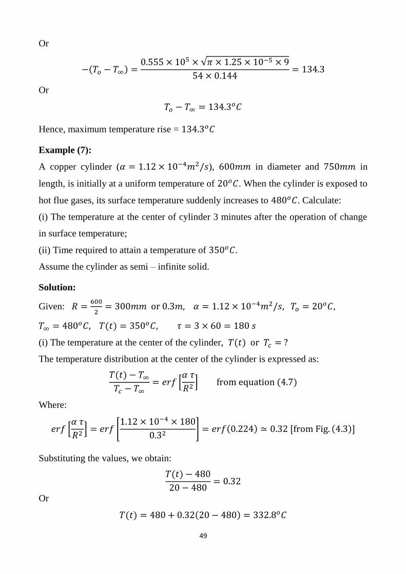
Example (7):

A copper cylinder (𝛼 = 1.12 × 10−4𝑚2/𝑠), 600𝑚𝑚 in diameter and 750𝑚𝑚 in

length, is initially at a uniform temperature of 20𝑜𝐶. When the cylinder is exposed to

hot flue gases, its surface temperature suddenly increases to 480𝑜𝐶. Calculate:

(i) The temperature at the center of cylinder 3 minutes after the operation of change

in surface temperature;

(ii) Time required to attain a temperature of 350𝑜𝐶.

Assume the cylinder as semi – infinite solid.

Solution:

Given: 𝑅 =600

2= 300𝑚𝑚 or 0.3𝑚, 𝛼 = 1.12 × 10−4𝑚2/𝑠, 𝑇𝑜 = 20𝑜𝐶,

𝑇∞ = 480𝑜𝐶, 𝑇(𝑡) = 350𝑜𝐶, 𝜏 = 3 × 60 = 180 𝑠

(i) The temperature at the center of the cylinder, 𝑇(𝑡) or 𝑇𝑐 = ?

The temperature distribution at the center of the cylinder is expressed as:

𝑇(𝑡) − 𝑇∞


𝛼 𝜏

𝑅2] from equation (4.7)

Where:

𝑒𝑟𝑓 [𝛼 𝜏

𝑅2] = 𝑒𝑟𝑓 [

1.12 × 10−4 × 180

0.32] = 𝑒𝑟𝑓(0.224) ≃ 0.32 [from Fig. (4.3)]

Substituting the values, we obtain:

𝑇(𝑡) − 480

20 − 480= 0.32

Or

𝑇(𝑡) = 480 + 0.32(20 − 480) = 332.8𝑜𝐶

50

(ii) Time required to attain a temperature of 350𝑜𝐶, 𝜏 =?

350 − 480

20 − 480= 𝑒𝑟𝑓 [

𝛼 𝜏

𝑅2]

0.2826 = 𝑒𝑟𝑓 [𝛼 𝜏

𝑅2]

∴ 𝛼 𝜏

𝑅2≃ 0.23

Or

𝜏 =0.23 × 𝑅2

𝛼=

0.23 × 0.32

1.12 × 10−4= 184.8 𝑠

51

Chapter Five

Systems with Periodic Variation of Surface Temperature

5.1 Introduction:

The periodic type of heat flow occurs in cyclic generators, in reciprocating

internal combustion engines and in the earth as the result of daily cycle of the sun.

These periodic changes, in general, are not simply sinusoidal but rather complex.

However, these complex changes can be approximated by a number of sinusoidal

components.

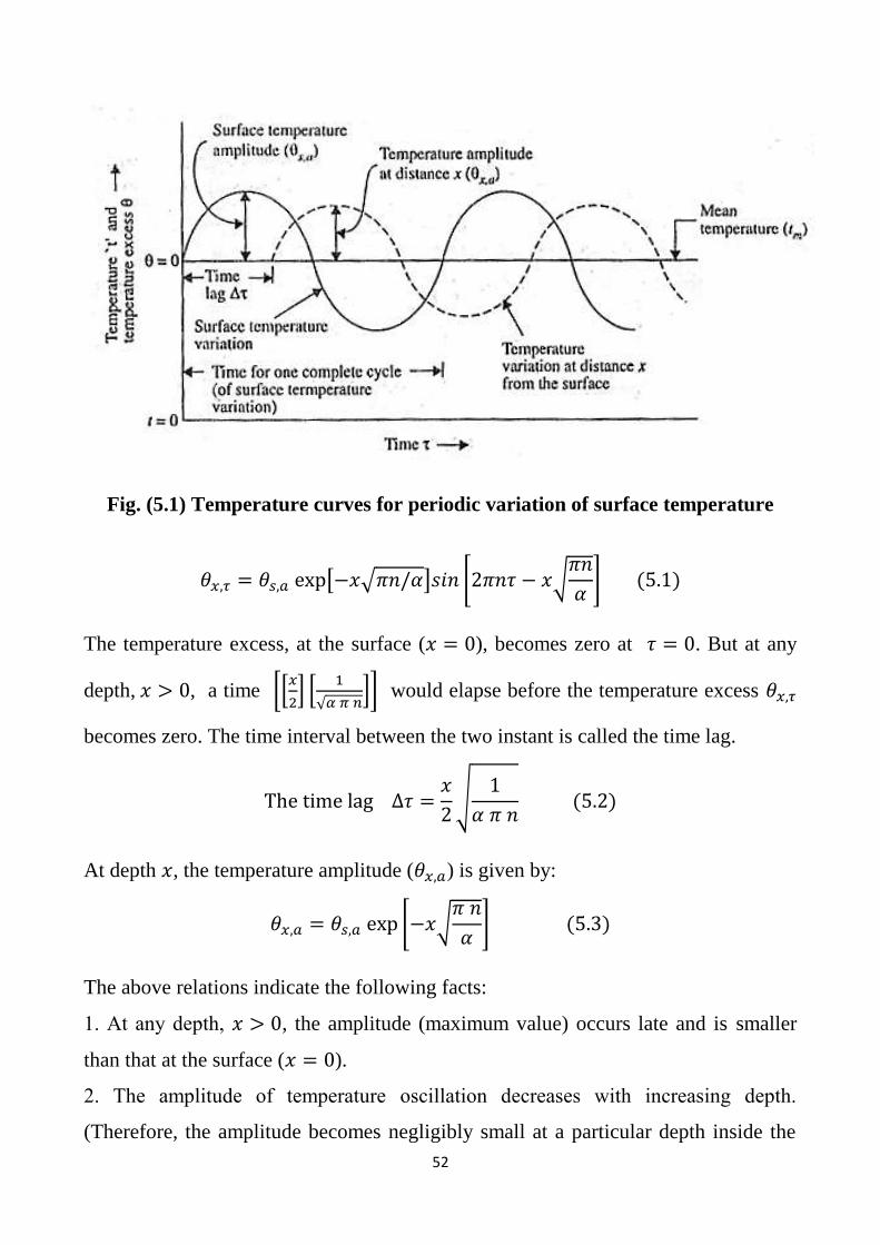
Let us consider a thick plane wall (one dimensional case) whose surface

temperature alters according to a sine function as shown in Fig. (5.1) below. The

surface temperature oscillates about the mean temperature level 𝑡𝑚 according to the

following relation:

𝜃𝑠,𝜏 = 𝜃𝑠,𝑎 sin (2𝜋𝑛𝜏)

Where,

𝜃𝑠,𝜏 = excess over the mean temperature (= 𝑡𝑠,𝜏 − 𝑡𝑚);

𝜃𝑠,𝑎 = Amplitude of temperature excess, i.e., the maximum temperature excess at the

surface;

𝑛 = Frequency of temperature wave.

The temperature excess at any depth 𝑥 and time 𝜏 can be expressed by the following

relation:

52

Fig. (5.1) Temperature curves for periodic variation of surface temperature

𝜃𝑥,𝜏 = 𝜃𝑠,𝑎 exp[−𝑥√𝜋𝑛/𝛼]𝑠𝑖𝑛 [2𝜋𝑛𝜏 − 𝑥√𝜋𝑛

𝛼] (5.1)

The temperature excess, at the surface (𝑥 = 0), becomes zero at 𝜏 = 0. But at any

depth, 𝑥 > 0, a time [[𝑥

2] [

1

√𝛼 𝜋 𝑛]] would elapse before the temperature excess 𝜃𝑥,𝜏

becomes zero. The time interval between the two instant is called the time lag.

The time lag ∆𝜏 =𝑥

2√

1

𝛼 𝜋 𝑛 (5.2)

At depth 𝑥, the temperature amplitude (𝜃𝑥,𝑎) is given by:

𝜃𝑥,𝑎 = 𝜃𝑠,𝑎 exp [−𝑥√𝜋 𝑛

𝛼] (5.3)

The above relations indicate the following facts:

1. At any depth, 𝑥 > 0, the amplitude (maximum value) occurs late and is smaller

than that at the surface (𝑥 = 0).

2. The amplitude of temperature oscillation decreases with increasing depth.

(Therefore, the amplitude becomes negligibly small at a particular depth inside the

53

solid and consequently a solid thicker than this particular depth is not of any

importance as far as variation in temperature is concerned).

3. With increasing value of frequency, time lag and the amplitude reduce.

4. Increase in diffusivity 𝛼 decreases the time lag but keeps the amplitude large.

5. The amplitude of temperature depends upon depth 𝑥 as well as the factor √𝑛

𝛼 .

Thus, if √𝑛

𝛼 is large, equation (5.3) holds good for thin solid rods also.


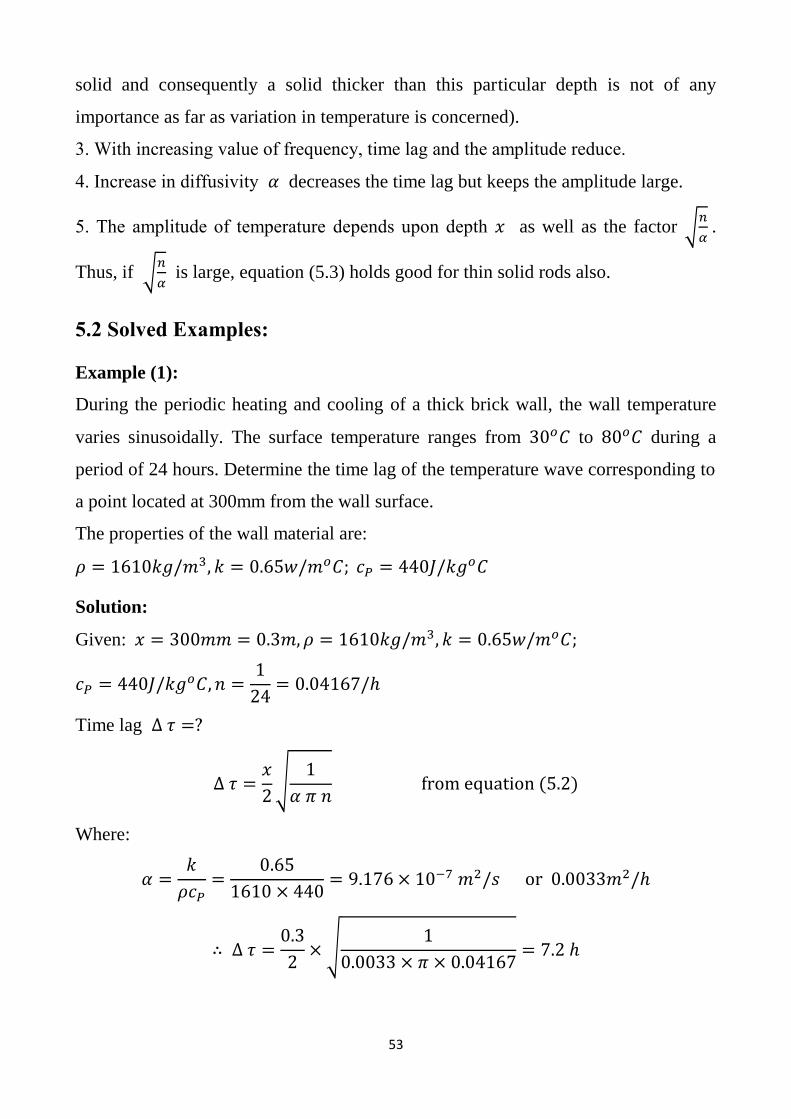
Example (1):

During the periodic heating and cooling of a thick brick wall, the wall temperature

varies sinusoidally. The surface temperature ranges from 30𝑜𝐶 to 80𝑜𝐶 during a

period of 24 hours. Determine the time lag of the temperature wave corresponding to

a point located at 300mm from the wall surface.

The properties of the wall material are:

𝜌 = 1610𝑘𝑔/𝑚3, 𝑘 = 0.65𝑤/𝑚𝑜𝐶; 𝑐𝑃 = 440𝐽/𝑘𝑔𝑜𝐶

Solution:

Given: 𝑥 = 300𝑚𝑚 = 0.3𝑚, 𝜌 = 1610𝑘𝑔/𝑚3, 𝑘 = 0.65𝑤/𝑚𝑜𝐶;

𝑐𝑃 = 440𝐽/𝑘𝑔𝑜𝐶, 𝑛 =1

24= 0.04167/ℎ

Time lag ∆ 𝜏 =?

∆ 𝜏 =𝑥

2√

1

𝛼 𝜋 𝑛 from equation (5.2)

Where:

𝛼 =𝑘

𝜌𝑐𝑃=

0.65

1610 × 440= 9.176 × 10−7 𝑚2/𝑠 or 0.0033𝑚2/ℎ

∴ ∆ 𝜏 =0.3

2× √

1

0.0033 × 𝜋 × 0.04167= 7.2 ℎ

54

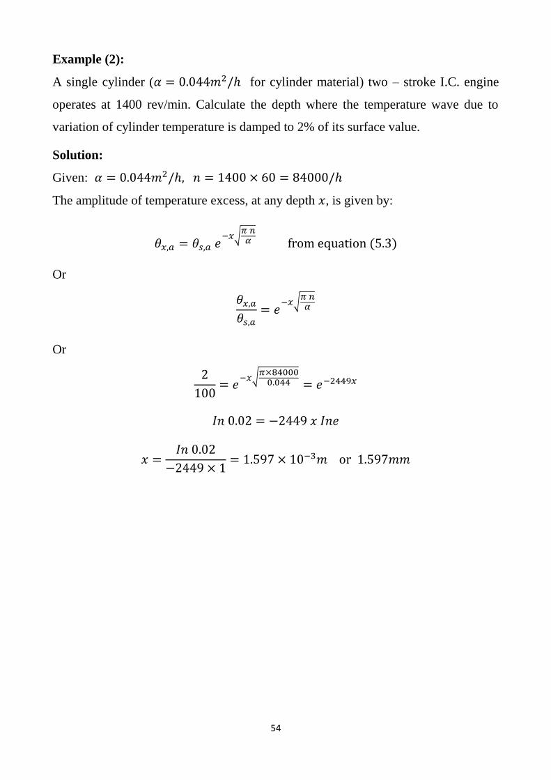
Example (2):

A single cylinder (𝛼 = 0.044𝑚2/ℎ for cylinder material) two – stroke I.C. engine

operates at 1400 rev/min. Calculate the depth where the temperature wave due to

variation of cylinder temperature is damped to 2% of its surface value.

Solution:

Given: 𝛼 = 0.044𝑚2/ℎ, 𝑛 = 1400 × 60 = 84000/ℎ

The amplitude of temperature excess, at any depth 𝑥, is given by:

𝜃𝑥,𝑎 = 𝜃𝑠,𝑎 𝑒−𝑥√

𝜋 𝑛𝛼 from equation (5.3)

Or

𝜃𝑥,𝑎

𝜃𝑠,𝑎= 𝑒

−𝑥√𝜋 𝑛𝛼

Or

2

100= 𝑒

−𝑥√𝜋×840000.044 = 𝑒−2449𝑥

𝐼𝑛 0.02 = −2449 𝑥 𝐼𝑛𝑒

𝑥 =𝐼𝑛 0.02

−2449 × 1= 1.597 × 10−3𝑚 or 1.597𝑚𝑚

55

Chapter Six

Transient Conduction with Given Temperature Distribution

6.1 Introduction:

The temperature distribution at some instant of time, in some situations, is

known for the one – dimensional transient heat conduction through a solid.

The known temperature distribution may be expressed in the form of polynomial

𝑡 = 𝑎 − 𝑏𝑥 + 𝑐𝑥2 + 𝑑𝑥3 − 𝑒𝑥4 Where 𝑎, 𝑏, 𝑐, 𝑑 and 𝑒 are the known coefficients.

By using such distribution, the one – dimensional transient heat conduction problem

can be solved.


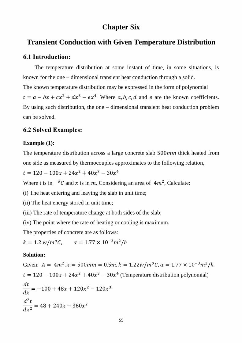
Example (1):

The temperature distribution across a large concrete slab 500𝑚𝑚 thick heated from

one side as measured by thermocouples approximates to the following relation,

𝑡 = 120 − 100𝑥 + 24𝑥2 + 40𝑥3 − 30𝑥4

Where t is in 𝑜𝐶 and 𝑥 is in 𝑚. Considering an area of 4𝑚2, Calculate:

(i) The heat entering and leaving the slab in unit time;

(ii) The heat energy stored in unit time;

(iii) The rate of temperature change at both sides of the slab;

(iv) The point where the rate of heating or cooling is maximum.

The properties of concrete are as follows:

𝑘 = 1.2 𝑤/𝑚𝑜𝐶, 𝛼 = 1.77 × 10−3𝑚2/ℎ

Solution:

Given: 𝐴 = 4𝑚2, 𝑥 = 500𝑚𝑚 = 0.5𝑚, 𝑘 = 1.22𝑤/𝑚𝑜𝐶, 𝛼 = 1.77 × 10−3𝑚2/ℎ

𝑡 = 120 − 100𝑥 + 24𝑥2 + 40𝑥3 − 30𝑥4 (Temperature distribution polynomial)

𝑑𝑡

𝑑𝑥= −100 + 48𝑥 + 120𝑥2 − 120𝑥3

𝑑2𝑡

𝑑𝑥2= 48 + 240𝑥 − 360𝑥2

56

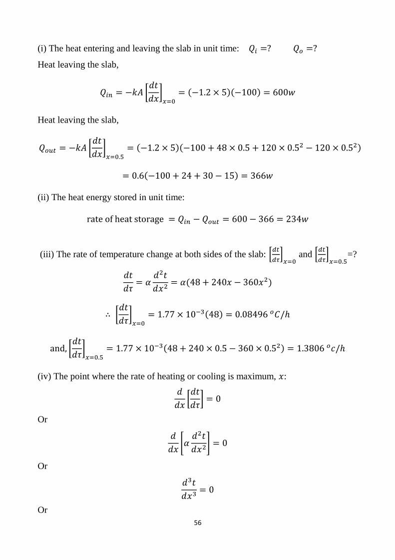
(i) The heat entering and leaving the slab in unit time: 𝑄𝑖 =? 𝑄𝑜 =?

Heat leaving the slab,

𝑄𝑖𝑛 = −𝑘𝐴 [𝑑𝑡

𝑑𝑥]

𝑥=0= (−1.2 × 5)(−100) = 600𝑤

Heat leaving the slab,

𝑄𝑜𝑢𝑡 = −𝑘𝐴 [𝑑𝑡

𝑑𝑥]

𝑥=0.5= (−1.2 × 5)(−100 + 48 × 0.5 + 120 × 0.52 − 120 × 0.52)

= 0.6(−100 + 24 + 30 − 15) = 366𝑤

(ii) The heat energy stored in unit time:

rate of heat storage = 𝑄𝑖𝑛 − 𝑄𝑜𝑢𝑡 = 600 − 366 = 234𝑤

(iii) The rate of temperature change at both sides of the slab: [𝑑𝑡

𝑑𝜏]

𝑥=0 and [

𝑑𝑡

𝑑𝜏]

𝑥=0.5=?

𝑑𝑡

𝑑𝜏= 𝛼

𝑑2𝑡

𝑑𝑥2= 𝛼(48 + 240𝑥 − 360𝑥2)

∴ [𝑑𝑡

𝑑𝜏]

𝑥=0= 1.77 × 10−3(48) = 0.08496 𝑜𝐶/ℎ

and, [𝑑𝑡

𝑑𝜏]

𝑥=0.5= 1.77 × 10−3(48 + 240 × 0.5 − 360 × 0.52) = 1.3806 𝑜𝑐/ℎ

(iv) The point where the rate of heating or cooling is maximum, 𝑥:

𝑑

𝑑𝑥[𝑑𝑡

𝑑𝜏] = 0

Or

𝑑

𝑑𝑥[𝛼

𝑑2𝑡

𝑑𝑥2] = 0

Or

𝑑3𝑡

𝑑𝑥3= 0

Or

57

240 − 720𝑥 = 0

∴ 𝑥 =240

720= 0.333𝑚

58

Chapter Seven

Additional Solved Examples in Lumped Capacitance System

7.1 Example (1): Determination of Temperature and Rate of Cooling

of a Steel Ball

A steel ball 100mm in diameter and initially at 900𝑜𝐶 is placed in air at 30𝑜𝐶, find:

(i) Temperature of the ball after 30 seconds.

(ii) The rate of cooling (𝑜𝐶/𝑚𝑖𝑛.) after 30 seconds.

Take: ℎ = 20𝑤/𝑚2𝑜𝐶; 𝑘(steel) = 40𝑤/𝑚𝑜𝐶; 𝜌(steel) = 7800𝑘𝑔/𝑚3;

𝑐𝑃(steel) = 460𝐽/𝑘𝑔𝑜𝐶

Solution:

Given: 𝑅 =100

2= 50𝑚𝑚 or 0.05𝑚; 𝑇𝑜 = 900𝑜𝐶; 𝑇∞ = 30𝑜𝐶, ℎ = 20𝑤/𝑚2𝑜

𝐶;

𝑘(steel) = 40𝑤/𝑚𝑜𝐶; 𝜌(steel) = 7800𝑘𝑔/𝑚3; 𝑐𝑃(steel) = 460𝐽/𝑘𝑔𝑜𝐶;

𝜏 = 30𝑠

(i) Temperature of the ball after 30 seconds: 𝑇(𝑡) =?


𝐿𝑐 =𝑉

𝐴𝑠=

43

𝜋𝑅3

4𝜋𝑅2=

𝑅

3=

0.05

3= 0.01667𝑚

Biot number,


𝑘=

20 × 0.01667

40= 0.008335

Since, 𝐵𝑖 is less than 0.1, hence lumped capacitance method (Newtonian heating or

cooling) may be applied for the solution of the problem.

The time versus temperature distribution is given by equation (1.4):

𝜃

𝜃𝑜=

𝑇(𝑡) − 𝑇∞

𝑇𝑜 − 𝑇∞= 𝑒

−ℎ𝐴𝑠𝜌𝑉𝑐𝑃 (1)

Now,

59

ℎ𝐴𝑠

𝜌𝑉𝑐𝑃∙ 𝜏 [

ℎ

𝜌𝑐𝑃] [

𝐴𝑠

𝑉] 𝜏 = [

20

7800 × 460] [

1

0.01667] (30) = 0.01

∴ 𝑇(𝑡) − 30

900 − 30= 𝑒−0.01 = 0.99

Or

𝑇(𝑡) = 30 + 0.99(900 − 30) = 891.3𝑜𝐶

(ii) The rate of cooling (𝑜𝐶/min) after 30 seconds: 𝑑𝑡

𝑑𝜏=?

The rate of cooling means we have to find out 𝑑𝑡

𝑑𝜏 at the required time. Now,

differentiating equation (1), we get:

1

𝑇𝑜 − 𝑇∞×

𝑑𝑡

𝑑𝜏= − [

ℎ𝐴𝑠

𝜌𝑣𝑐𝑃] 𝑒

−ℎ𝐴𝑠𝜌𝑉𝑐𝑃

𝜏

Now, substituting the proper values in the above equation, we have:

1

(900 − 30)∙

𝑑𝑡

𝑑𝜏= − [

20

7800 × 460×

1

0.01667] × 0.99 = −3.31 × 10−4

∴ 𝑑𝑡

𝑑𝜏= (900 − 30)(−3.31 × 10−4) = −0.288𝑜𝐶/𝑠

𝑜𝑟 𝑑𝑡

𝑑𝜏= −0.288 × 60 = −17.28𝑜𝑐/𝑚𝑖𝑚

7.2 Example (2): Calculation of the Time Required to Cool a Thin

Copper Plate

A thin copper plate 20𝑚𝑚 thick is initially at 150𝑜𝐶. One surface is in contact with

water at 30𝑜𝑐 (ℎ𝑤 = 100𝑤/𝑚2𝑜𝐶) and the other surface is exposed to air at 30𝑜𝐶

(ℎ𝑎 = 20𝑤/𝑚2𝑜𝐶). Determine the time required to cool the plate to 90𝑜𝐶.

Take the following properties of the copper:

𝜌 = 8800𝑘𝑔/𝑚3; 𝑐𝑃 = 400𝐽/𝑘𝑔𝑜𝐶 𝑎𝑛𝑑 𝑘 = 360𝑤/𝑚𝑜𝐶

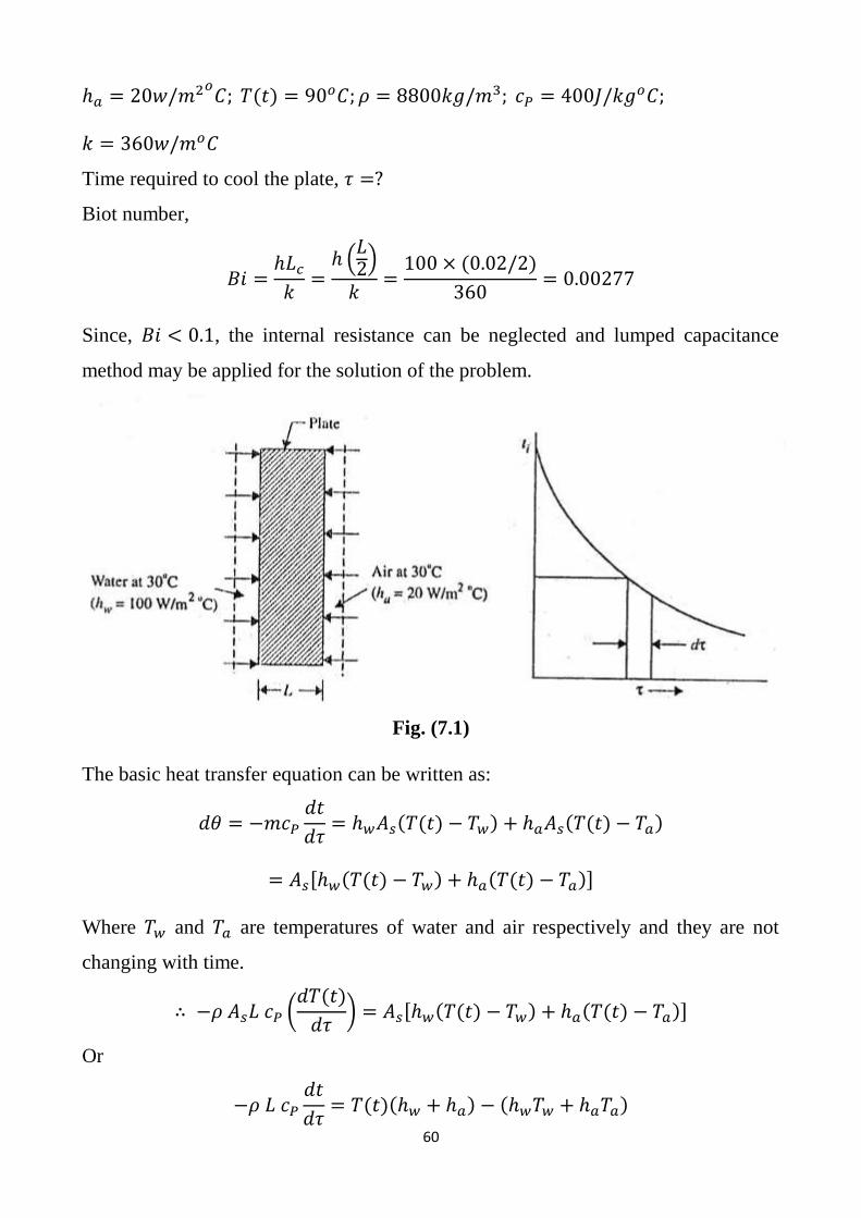
The plate is shown in Fig. (7.1) below:

Solution:

Given: 𝐿 = 20𝑚𝑚 or 0.02𝑚; 𝑇𝑜 = 150𝑜𝐶; 𝑇∞ = 30𝑜𝐶, ℎ𝑤 = 100𝑤/𝑚2𝑜𝐶;

60

ℎ𝑎 = 20𝑤/𝑚2𝑜𝐶; 𝑇(𝑡) = 90𝑜𝐶; 𝜌 = 8800𝑘𝑔/𝑚3; 𝑐𝑃 = 400𝐽/𝑘𝑔𝑜𝐶;

𝑘 = 360𝑤/𝑚𝑜𝐶

Time required to cool the plate, 𝜏 =?

Biot number,


𝑘=

ℎ (𝐿2)

𝑘=

100 × (0.02/2)

360= 0.00277

Since, 𝐵𝑖 < 0.1, the internal resistance can be neglected and lumped capacitance

method may be applied for the solution of the problem.

Fig. (7.1)

The basic heat transfer equation can be written as:

𝑑𝜃 = −𝑚𝑐𝑃

𝑑𝑡

𝑑𝜏= ℎ𝑤𝐴𝑠(𝑇(𝑡) − 𝑇𝑤) + ℎ𝑎𝐴𝑠(𝑇(𝑡) − 𝑇𝑎)

= 𝐴𝑠[ℎ𝑤(𝑇(𝑡) − 𝑇𝑤) + ℎ𝑎(𝑇(𝑡) − 𝑇𝑎)]

Where 𝑇𝑤 and 𝑇𝑎 are temperatures of water and air respectively and they are not

changing with time.

∴ −𝜌 𝐴𝑠𝐿 𝑐𝑃 (𝑑𝑇(𝑡)

𝑑𝜏) = 𝐴𝑠[ℎ𝑤(𝑇(𝑡) − 𝑇𝑤) + ℎ𝑎(𝑇(𝑡) − 𝑇𝑎)]

Or

−𝜌 𝐿 𝑐𝑃

𝑑𝑡

𝑑𝜏= 𝑇(𝑡)(ℎ𝑤 + ℎ𝑎) − (ℎ𝑤𝑇𝑤 + ℎ𝑎𝑇𝑎)

61

Or

𝑑𝑇(𝑡)

𝑇(𝑡)(ℎ𝑤 + ℎ𝑎) − (ℎ𝑤𝑇𝑤 + ℎ𝑎𝑇𝑎)=

𝑑𝜏

𝜌 𝐿 𝑐𝑃

Or

𝑑𝑇(𝑡)

𝑐1𝑇(𝑡) − 𝑐2= −

𝑑𝜏

𝜌 𝐿 𝑐𝑃

Where

𝑐1 = ℎ𝑤 + ℎ𝑎 and 𝑐2 = ℎ𝑤𝑇𝑤 + ℎ𝑎𝑇𝑎

∴ 1

𝑐1∫

𝑑𝑇(𝑡)

𝑇(𝑡) −𝑐2

𝑐1

= − ∫𝑑𝜏

𝜌 𝐿 𝑐𝑃

Or

1

𝑐1∫

𝑑𝑇(𝑡)

𝑇(𝑡) −𝑐2

𝑐1

= − ∫𝑑𝜏

𝜌 𝐿 𝑐𝑃

𝜏

0

where 𝑐 =𝑐2

𝑐1

𝑇(𝑡)

𝑇𝑜

Or

1

𝑐1

[ln(𝑇(𝑡) − 𝑐)]𝑇𝑜

𝑇(𝑡)= −

𝜏

𝜌 𝐿 𝑐𝑃

Or

1

𝑐1

[ln(𝑇(𝑡) − 𝑐)]𝑇(𝑡)𝑇𝑜 =

𝜏

𝜌 𝐿 𝑐𝑃

Or

𝜏 =𝜌 𝐿 𝑐𝑃

𝑐1ln [

𝑇𝑜 − 𝑐

𝑇(𝑡) − 𝑐] (1)

𝑐1 = ℎ𝑤 + ℎ𝑎 = 100 + 20 = 120

𝑐2 = ℎ𝑤𝑇𝑤 + ℎ𝑎𝑇𝑎 = 100 × 30 + 20 × 30 = 3600

𝑐 =𝑐2

𝑐1=

3600

120= 30

Substituting the proper values in equation (1), we get:

62

𝜏 =8800 × 0.02 × 400

120ln [

150 − 30

90 − 30] = 406.6 𝑠 or 6.776 minutes

7.3 Example (3): Determining the Conditions under which the Contact

Surface Remains at Constant Temperature

Two infinite bodies of thermal conductivities 𝑘1 and 𝑘2, thermal diffusivities 𝛼1 and

𝛼2 are initially at temperatures 𝑡1 and 𝑡2 respectively. Each body has single plane

surface and these surfaces are placed in contact with each other. Determine the

conditions under which the contact surface remains at constant temperature 𝑡𝑠 where

𝑡1 > 𝑡𝑠 > 𝑡2 .

Solution:

The rate of heat flow at a surface (𝑥 = 0) is given by,

𝑄 =−𝑘𝐴∆𝑡

√𝜋 𝛼 𝜏

Heat received by each unit area of contact surface from the body at temperature 𝑡1 is,

𝑄1 =−𝑘1(𝑡1 − 𝑡𝑠)

√𝜋 𝛼1 𝜏

Heat lost by each unit area of contact surface from the body at temperature 𝑡2 is,

𝑄2 =−𝑘2(𝑡𝑠 − 𝑡2)

√𝜋 𝛼2 𝜏

The contact surface will remain at a constant temperature if:

−𝑘1(𝑡1 − 𝑡𝑠)

√𝜋 𝛼1 𝜏=

−𝑘2(𝑡𝑠 − 𝑡2)

√𝜋 𝛼2 𝜏

Or

𝑘1(𝑡1 − 𝑡𝑠)

√ 𝛼1

=𝑘2(𝑡𝑠 − 𝑡2)

√ 𝛼2

Or

𝑘1(𝑡1 − 𝑡𝑠)√𝛼2 = 𝑘2(𝑡𝑠 − 𝑡2)√𝛼1

Or

𝑘1𝑡1√𝛼2 − 𝑘1𝑡𝑠√𝛼2 = 𝑘2𝑡𝑠√𝛼1 − 𝑘2𝑡2√𝛼1

63

Or

𝑡𝑠(𝑘1√𝛼2 + 𝑘2√𝛼1) = 𝑘1𝑡1√𝛼2 + 𝑘2𝑡2√𝛼1

Or

𝑡𝑠 =𝑘1𝑡1√𝛼2 + 𝑘2𝑡2√𝛼1

𝑘1√𝛼2 + 𝑘2√𝛼1

By dividing the numerator and the denominator by √𝛼1 𝛼2, the following formula is

obtained:

𝑡𝑠 =(𝑘1𝑡1/√𝛼1) + (𝑘2𝑡2/√𝛼2)

(𝑘1/√𝛼1) + (𝑘2/√𝛼2)

7.4 Example (4): Calculation of the Time Required for the Plate to


A 50𝑐𝑚 × 50𝑐𝑚 copper slab 6.25mm thick has a uniform temperature of 300𝑜𝐶. Its

temperature is suddenly lowered to 36𝑜𝐶. Calculate the time required for the plate to

reach the temperature of 108𝑜𝐶.

Take: 𝜌 = 9000𝑘𝑔/𝑚3; 𝑐𝑃 = 0.38𝑘𝐽/𝑘𝑔𝑜𝐶; 𝑘 = 370𝑤/𝑚𝑜𝐶 and ℎ = 90𝑤/𝑚2𝑜𝐶

Solution:

Surface area of plate (two sides),

𝐴𝑠 = 2 × 0.5 × 0.5 = 0.5𝑚2

Volume of plate,

𝑉 = 0.5 × 0.5 × 0.00625 = 0.0015625𝑚3


𝐿 =𝑉

𝐴𝑠=

0.0015625

0.5= 0.003125 𝑚

𝐵𝑖 =ℎ𝐿

𝑘=

90 × 0.003125

370= 7.6 × 10−4

Since, 𝐵𝑖 ≪ 0.1 , hence lumped capacitance method (Newtonian heating or cooling)

may be applied for the solution of the problem.

64


𝜃

𝜃𝑜=

𝑇(𝑡) − 𝑇∞


𝐹𝑜 =𝑘


370

9000 × 0.38 × 103 × 0.0031252∙ 𝜏 = 11.0784 𝜏

𝜃

𝜃𝑜=

108 − 36

300 − 36= 𝑒−7.6×10−4×11.0784 𝜏 = 𝑒−8.42×10−3 𝜏

0.27273 = 𝑒−8.42×10−3 𝜏

ln 0.27273 = −8.42 × 10−3 𝜏 ln 𝑒

𝜏 =ln 0.27273

−8.42 × 10−3 ln 𝑒= 154.31 𝑠

7.5 Example (5): Determination of the Time Required for the Plate to


An aluminum alloy plate of 400𝑚𝑚 × 400𝑚𝑚 × 4𝑚𝑚 size at 200𝑜𝐶 is suddenly

quenched into liquid oxygen at −183𝑜𝐶. Starting from fundamentals or deriving the

necessary expression, determine the time required for the plate to reach a temperature

of −70𝑜𝐶. Assume ℎ = 20000𝑘𝐽/𝑚2 ∙ ℎ𝑟 ∙𝑜 𝐶

𝑐𝑃 = 0.8𝑘𝐽/𝑘𝑔𝑜𝐶 , and 𝜌 = 3000𝑘𝑔/𝑚3, 𝑘 for aluminum at low temperature

may be taken as 214𝑤/𝑚𝑜𝐶 𝑜𝑟 770.4 𝑘𝐽/𝑚ℎ𝑜𝐶

Solution:

Surface area of the plate,

𝐴𝑠 = 2 × 0.4 × 0.4 = 0.32𝑚2

Volume of the plate,

𝑉 = 0.4 × 0.4 × 0.004 = 0.00064𝑚3


𝐿 =𝑡

2=

0.004

2= 0.002 𝑚

65

Or 𝐿 =𝑉

𝐴𝑠=

0.00064

0.32= 0.002 𝑚

𝑘 for aluminum, at low temperature may be taken as 214𝑤/𝑚𝑜𝐶 or 770.4𝑘𝐽/𝑚ℎ𝑜𝑐

∴ 𝐵𝑖 =ℎ𝐿

𝑘=

2000 × 0.002

770.4= 0.0519

Since, 𝐵𝑖 ≪ 0.1, hence lumped capacitance method may be applied for the solution

of the problem.


𝜃

𝜃𝑜=

𝑇(𝑡) − 𝑇∞


𝐹𝑜 =𝑘


214

3000 × 0.8 × 103 × 0.0022∙ 𝜏 = 22.3 𝜏

𝐵𝑖 × 𝐹𝑜 = 0.0519 × 22.3 = 1.15737 𝜏

∴𝜃

𝜃𝑜=

−70 − (−183)

200 − (−183)== 𝑒−1.15737 𝜏

113

383= 𝑒−1.15737 𝜏

0.295 = 𝑒−1.15737 𝜏

ln 0.295 = −1.15737 𝜏 ln 𝑒

𝜏 =ln 0.295

−1.15737 × 1= 1.055 𝑠

7.6 Example (6): Determining the Temperature of a Solid Copper

Sphere at a Given Time after the Immersion in a Well – Stirred Fluid

A solid copper sphere of 10𝑐𝑚 diameter (𝜌 = 8954𝑘𝑔/𝑚3, 𝑐𝑝 = 383𝐽/𝑘𝑔, 𝐾 =

386𝑤/𝑚𝐾) initially at a uniform temperature of 𝑇𝑜 = 250𝑜𝐶, is suddenly immersed

in a well – stirred fluid which is maintained at a uniform temperature 𝑇∞ = 50𝑜𝐶.

66

The heat transfer coefficient between the sphere and the fluid is ℎ = 200𝑤/𝑚2𝐾.

Determine the temperature of the copper block at 𝜏 = 5 𝑚𝑖𝑛. after the immersion.

Solution:

Given: 𝑑 = 10𝑐𝑚 = 0.1𝑚; 𝜌 = 8954𝑘𝑔/𝑚3; 𝑐𝑝 = 383𝐽/𝑘𝑔 𝑘; 𝑘 = 386𝑤/𝑚 𝐾,

𝑇𝑜 = 250𝑜𝐶; 𝑇∞ = 50𝑜𝐶; ℎ = 200𝑤/𝑚2𝐾; 𝜏 = 5𝑚𝑖𝑛 = 5 × 60 = 300 𝑠

Temperature of the copper block, 𝑇(𝑡) = ?

The characteristic length of the sphere is,

𝐿 =𝑉

𝐴𝑠=

43

𝜋𝑟3

4𝜋𝑟2=

𝑟

3=

𝑑

6=

0.1

6= 0.01667𝑚

𝐵𝑖 =ℎ𝐿

𝑘=

200 × 0.01667

386= 8.64 × 10−3

Since, 𝐵𝑖 ≪ 0.1 , hence lumped capacitance method (Newtonian heating or cooling)

may be applied for the solution of the problem.


𝜃

𝜃𝑜=

𝑇(𝑡) − 𝑇∞


𝐹𝑜 =𝑘


386

8954 × 383 × 0.016672 × 300= 121.513

𝐵𝑖 × 𝐹𝑜 = 8.64 × 10−3 × 121.513 = 1.05

∴𝜃

𝜃𝑜=

−𝑇(𝑡) − 50

250 − 50= 𝑒−1.05

𝑇(𝑡) − 50 = 200 𝑒−1.05

∴ 𝑇(𝑡) = 50 + 200 𝑒−1.05 = 50 + 70 = 120𝑜𝑐

7.7 Example (7): Determination of the Heat Transfer Coefficient

An average convective heat transfer coefficient for flow of 90𝑜𝐶 air over a plate is

measured by observing the temperature – time history of a 40𝑚𝑚 thick copper slab

(𝜌 = 9000𝑘𝑔/𝑚3, 𝑐𝑝 = 0.38𝑘𝑗/𝑘𝑔𝑜𝐶, 𝑘 = 370𝑤/𝑚𝑜𝐶) exposed to 90𝑜𝐶 air. In

67

one test run, the initial temperature of the plate was 200𝑜𝐶, and in 4.5 minutes the

temperature decreased by 35𝑜𝐶. Find the heat transfer coefficient for this case.

Neglect internal thermal resistance.

Solution:

Given: 𝑇∞ = 90𝑜𝐶; 𝑡 = 40𝑚𝑚 𝑜𝑟 0.04𝑚; 𝜌 = 9000𝑘𝑔/𝑚3; 𝑐𝑝 = 0.38𝑘𝑗/𝑘𝑔𝑜𝐶;

𝑇𝑜 = 200𝑜𝐶; 𝑇(𝑡) = 200 − 35 = 165𝑜𝐶; 𝜏 = 4.5𝑚𝑖𝑛 = 270𝑠

Characteristic length of the sphere is,

𝐿 =𝑡

2=

0.04

2= 0.02𝑚

𝐵𝑖 =ℎ𝐿

𝑘=

0.02ℎ

370= 5.405 × 10−5ℎ

𝐹𝑜 =𝑘


370

9000 × 0.38 × 103 × 0.022× 270 = 73.03

𝐵𝑖 × 𝐹𝑜 = 5.405 × 10−5 × 73.03ℎ = 394.73 × 10−5ℎ = 0.003947ℎ

𝜃

𝜃𝑜=

𝑇(𝑡) − 𝑇∞


𝜃

𝜃𝑜=

165 − 90

200 − 90= 𝑒−0.003947ℎ

0.682 = 𝑒−0.003947ℎ

ln 0.682 = −0.003947ℎ ln 𝑒

ℎ =ln 0.682

−0.003947 × 1= 96.97𝑤/𝑚2𝑜

𝐶

7.8 Example (8): Determination of the Heat Transfer Coefficient

The heat transfer coefficients for flow of air at 28𝑜𝐶 over a 12.5𝑚𝑚 diameter sphere

are measured by observing the temperature – time history of a copper ball of the same

dimension. The temperature of the copper ball (𝑐𝑝 = 0.4𝑘𝑗/𝑘𝑔 𝐾 and 𝜌 =

8850𝑘𝑔/𝑚3) was measured by two thermo – couples, one located in the center and

68

the other near the surface. Both the thermocouples registered the same temperature at

a given instant. In one test the initial temperature of the ball was 65𝑜𝐶, and in 1.15

minutes the temperature decreased by 11𝑜𝐶 . Calculate the heat transfer coefficient

for this case.

Solution:

Given: 𝑇∞ = 28𝑜𝐶; 𝑟(sphere) =12.5

2= 6.25𝑚𝑚 = 0.00625𝑚; 𝑐𝑝 = 0.4𝑘𝑗/𝑘𝑔 𝐾;

𝜌 = 8850𝑘𝑔/𝑚3; 𝑇𝑜 = 65𝑜𝐶; 𝑇(𝑡) = 65 − 11 = 54𝑜𝐶; 𝜏 = 1.15𝑚𝑖𝑛 = 69 𝑠;

𝐵𝑖 =ℎ𝐿

𝑘; characteristic length 𝐿 =

𝑉

𝐴𝑠=

𝑟

3=

0.00625

3= 2.083 × 10−3

Since, heat transfer coefficient has to be calculated, so assume that the internal

resistance is negligible and 𝐵𝑖 is much less than 0.1 .

𝐵𝑖 =ℎ𝑟

3𝑘=

0.00625ℎ

3𝑘=

2.083 × 10−3ℎ

𝑘

𝐹𝑜 =𝑘


𝑘

8850 × 0.4 × 103 × (2.083 × 10−3)2× 270

= 0.0651 𝑘 × 69 = 4.5 𝑘

𝐵𝑖 × 𝐹𝑜 =0.00625ℎ

3𝑘× 4.5𝑘 = 9.375 × 10−3ℎ

𝜃

𝜃𝑜=

𝑇(𝑡) − 𝑇∞


𝜃

𝜃𝑜=

54 − 28

65 − 28= 𝑒−9.375×10−3ℎ

0.7027 = 𝑒−0.009375ℎ

ln 0.7027 = −0.009375ℎ ln 𝑒

∴ ℎ =ln 0.7027

−0.009375 × 1= 37.63𝑤/𝑚2𝐾

69

7.9 Example (9): Calculation of the Initial Rate of Cooling of a Steel

Ball

A steel ball 50mm in diameter and at 900𝑜𝐶 is placed in still atmosphere of 30𝑜𝐶.

Calculate the initial rate of cooling of the ball in 𝑜𝐶/𝑚𝑖𝑛, if the duration of cooling is

1 minute.

Take: 𝜌 = 7800𝑘𝑔/𝑚3; 𝑐𝑝 = 2𝑘𝑗/𝑘𝑔𝑜𝐶 (for steel); ℎ = 30𝑤/𝑚2𝑜𝐶.


Solution:

Given: 𝑟 =50

2= 25𝑚𝑚 = 0.025𝑚; 𝑇𝑜 = 900𝑜𝐶; 𝑇∞ = 30𝑜𝐶; 𝜌 = 7800𝑘𝑔/𝑚3

𝑐𝑝 = 2𝑘𝑗/𝑘𝑔𝑜𝐶; ℎ = 30𝑤/𝑚2𝑜𝐶; 𝜏 = 1𝑚𝑖𝑛 = 60 𝑠;

The temperature variation in the ball (with respect to time), neglecting internal

thermal resistance, is given by:

𝜃

𝜃𝑜=

𝑇(𝑡) − 𝑇∞


𝐵𝑖 =ℎ𝐿

𝑘, 𝐿 of a ball =

𝑟

3=

0.025

3

∴ 𝐵𝑖 =ℎ𝑟

3𝑘=

30 × 0.025

3𝑘=

0.25

𝑘

𝐹𝑜 =𝑘


𝑘

7800 × 2 × 103 × (0.025/3)2⋅ 𝜏

𝐹𝑜 = 9.23 × 10−4 × 60 = 0.0554𝑘

𝐵𝑖 × 𝐹𝑜 =0.25

𝑘× 0.0554𝑘 = 0.01385

𝜃

𝜃𝑜=

𝑇(𝑡) − 30

900 − 30= 𝑒−0.01385

𝑇(𝑡) = 870 𝑒−0.01385 + 30 = 888𝑜𝐶

∴ rate of cooling = 900 − 888

1 𝑚𝑖𝑛= 12𝑜𝐶/𝑚𝑖𝑛

70

7.10 Example (10): Determination of the Maximum Speed of a

Cylindrical Ingot inside a Furnace

A cylinder ingot 10𝑐𝑚 diameter and 30𝑐𝑚 long passes through a heat treatment

furnace which is 6m in length. The ingot must reach a temperature of 800𝑜𝐶 before it

comes out of the furnace. The furnace gas is at 1250𝑜𝐶 and the ingot initial

temperature is 90𝑜𝐶. What is the maximum speed with which the ingot should move

in the furnace to attain the required temperature? The combined radiative and

convective surface heat transfer coefficient is 100𝑤/𝑚2𝑜𝐶.

Take: k (steel) = 40𝑤/𝑚2𝑜𝐶 and 𝛼 (thermal diffusivity of steel) = 1.16 × 10−5𝑚2/𝑠.

Solution:

𝑑 = 10𝑐𝑚 = 0.1𝑚; 𝐿 = 30𝑐𝑚 = 0.3𝑚; Length of the furnace = 6𝑚;

𝑇𝑜 = 800𝑜𝐶; 𝑇(𝑡) = 800𝑜𝐶; 𝑇∞ = 90𝑜𝐶;

𝑣𝑚𝑎𝑥 of ingot passing through the furnace =?

ℎ = 100𝑤/𝑚2𝑜𝐶; 𝑘(steel) = 40𝑤/𝑚𝑜𝐶; 𝛼(steel) = 1.16 × 10−5𝑚2/𝑠


𝐿𝑐 =𝑉

𝐴𝑠=

43

𝑑2𝐿

[𝜋𝑑𝐿 +𝜋4

𝑑2 × 2]=

𝑑𝐿

4𝐿 + 2𝑑

=0.1 × 0.3

4 × 0.3 + 2 × 0.1= 0.02143𝑚


𝑘=

100 × 0.02143

40= 0.0536

As 𝐵𝑖 ≪ 0.1 , Then internal thermal resistance of the ingot for conduction heat flow

can be neglected.

The time versus temperature relation is given as:

𝑇(𝑡) − 𝑇∞


𝐹𝑜 =𝑘


𝛼

𝐿2∙ 𝜏 =

1.16 × 10−5

0.021432∙ 𝜏 = 0.02526 𝜏

71

𝐵𝑖 × 𝐹𝑜 = 0.0536 × 0.02526 𝜏 = 1.35410−3𝜏 = 0.001354 𝜏

𝜃

𝜃𝑜=

𝑇(𝑡) − 𝑇∞


𝜃

𝜃𝑜=

800 − 90

1250 − 90= 𝑒−0.001354 𝜏

0.6121 = 𝑒−0.001354 𝜏

−0.001354 𝜏 ln 𝑒 = ln 0.6121

𝜏 =ln 0.6121

−0.001354= 362.5 𝑠

𝑣𝑚𝑎𝑥 of ingot passing through the furnace,

𝑣𝑚𝑎𝑥 =furnace length

time=

6

362.5= 0.01655𝑚/𝑠

7.11 Example (11): Determining the Time Required to Cool a Mild

Steel Sphere, the Instantaneous Heat Transfer Rate, and the Total

Energy Transfer

A 15𝑚𝑚 diameter mild steel sphere (𝑘 = 4.2𝑤/𝑚𝑜C is exposed to cooling air flow

at 20𝑜𝑐 resulting in the convective, coefficient ℎ = 120𝑤/𝑚2𝑜𝐶.

Determine the following:

(i) Time required to cool the sphere from 550𝑜𝐶 to 90𝑜𝐶 .

(ii) Instantaneous heat transfer rate 2 minutes after the start of cooling.

(iii) Total energy transferred from the sphere during the first 2 minutes.

For mild steel take: 𝜌 = 7850𝑘𝑔/𝑚3; 𝑐𝑝 = 475𝐽/𝑘𝑔𝑜𝐶; and 𝛼 = 0.045 𝑚2/ℎ

Solution:

Given: 𝑟 =15

2= 7.5𝑚𝑚 = 0.0075𝑚; 𝑘 = 42𝑤/𝑚2𝑜

𝐶; 𝑇∞ = 20𝑜𝐶; 𝑇𝑜 = 550𝑜𝐶;

𝑇(𝑡) = 90𝑜𝐶; ℎ = 120𝑤/𝑚2𝑜𝐶;

(i) Time required to cool the sphere from 550𝑜𝐶 to 90𝑜𝐶, 𝜏 = ?

The characteristic length, 𝐿𝑐 is given by,

72

𝐿𝑐 =𝑟

3=

0.0075

3= 0.0025𝑚

Biot number,


𝑘=

120 × 0.0025

42= 0.007143

Since, 𝐵𝑖 ≪ 0.1 , so we can use the lumped capacitance theory to solve this problem.

Fourier Number,

𝐹𝑜 =𝑘


𝛼

𝐿𝑐2

∙ 𝜏

𝛼 = 0.045𝑚2/ℎ =0.045

3600= 1.25 × 10−5𝑚2/𝑠

𝐹𝑜 =1.25 × 10−5

(0.0025)2∙ 𝜏 = 2𝜏

𝐵𝑖 × 𝐹𝑜 = 0.007143 × 2𝜏

The temperature variation with time is given by:

𝜃

𝜃𝑜=

𝑇(𝑡) − 𝑇∞


=90 − 20

550 − 20= 𝑒−0.014286 𝜏

0.132 = 𝑒−0.014286 𝜏

−0.014286 𝜏 ln 𝑒 = ln 0.132

𝜏 =ln 0.132

−0.014286= 141.7 𝑠

(ii) Instantaneous heat transfer rate 2 minutes (0.0333h) after the start of cooling,

𝑞′(𝜏) =?

𝑞′(𝜏) = ℎ𝐴𝑠𝜃𝑜𝑒−𝐵𝑖×𝐹𝑜

𝐵𝑖 × 𝐹𝑜 = 0.014286 × 2 × 60 = 1.7143

73

𝑞′(𝜏) = 120 × 4𝜋 × (0.0075)2(550 − 20)𝑒−1.7143 = 8.1𝑤

(iii) Total energy transferred from the sphere during the first 2 minutes, (0.0333h)

𝑄(𝑡) = ?



= 120 × 4𝜋 × (0.0075)2(550 − 20)[1 − 𝑒−1.7143] ×120

1.7143= 2580.2 𝐽

Or

𝐹𝑜 =𝑘

𝜌𝑐𝑃𝐿𝑐2

⋅ 𝜏 =𝑘

7850 × 475 × 0.00252× 120 = 206

𝐵𝑖 × 𝐹𝑜 = 0.007143 × 206 = 1.471

𝑄(𝑡) = 120 × 4𝜋 × (0.0075)2(550 − 20)[1 − 𝑒−1.471] ×120

1.471= 2825 𝐽

7.12 Example (12): Estimation of the Time Required to Cool a

Decorative Plastic Film on Copper Sphere to a Given Temperature

using Lumped Capacitance Theory

The decorative plastic film on copper sphere 10mm in diameter is cured in an oven at

75𝑜𝐶. After removal from oven, the sphere is exposed to an air stream at 10m/s and

23𝑜𝐶. Estimate the time taken to cool the sphere to 35𝑜𝐶 using lumped capacitance

theory.

Use the following correlation:

𝑁𝑢 = 2 + [0.4(𝑅𝑒)0.5 + 0.06(𝑅𝑒)2/3](𝑝𝑟)0.4 [𝜇𝑎

𝜇𝑠]

0.25

For determination of correlation coefficient ℎ, use the following properties of air and

copper:

For copper: 𝜌 = 8933𝑘𝑔/𝑚3; 𝑘 = 400𝑤/𝑚 𝐾; 𝑐𝑝 = 380𝐽/𝑘𝑔𝑜𝐶

For air at 23𝑜𝐶: 𝜇𝑎 = 18.6 × 10−6𝑁𝑠/𝑚2, 𝜈 = 15.36 × 10−6𝑚2/𝑠

𝑘 = 0.0258𝑤/𝑚 𝐾, 𝑝𝑟 = 0.709, and

𝜇𝑠 = 19.7 × 10−6𝑁𝑠/𝑚2, at 35𝑜𝐶

74

Solution:

𝑑 = 10𝑚𝑚 = 0.01𝑚; 𝑇𝑜 = 75𝑜𝐶; 𝑣 = 10𝑚/𝑠; 𝑇∞ = 23𝑜𝐶; 𝑇(𝑡) = 35𝑜𝐶;

Time taken to cool the sphere, 𝜏 = ?

𝑅𝑒 =𝑣 𝑑

𝜈=

10 × 0.01

15.36 × 10−6= 6510

𝑁𝑢 = 2 + [0.4(6510)0.5 + 0.06(6510)2/3] × (0.709)0.4 × [18.16 × 10−6

19.78 × 10−6]

0.25

= 2 + [32.27 + 20.92] × 0.87 × 0.979 = 47.3

𝑜𝑟 𝑁𝑢 =ℎ 𝑑

𝑘= 47.3

∴ ℎ =𝑘

𝑑𝑁𝑢 =

0.0258

0.01× 47.3 = 122𝑤/𝑚2𝑜

𝐶

The time taken to cool from 75𝑜𝐶 to 35𝑜𝐶 may be found from the following relation:

𝜃

𝜃𝑜=

𝑇(𝑡) − 𝑇∞


𝐵𝑖 =ℎ 𝐿

𝑘

The characteristic length of a sphere, 𝐿 = 𝑟

3=

0.005

3𝑚

𝐵𝑖 =ℎ 𝐿

𝑘=

122 × 0.005

3 × 400= 5.083 × 10−4

Since, 𝐵𝑖 ≪ 0.1 , so we can use the lumped capacitance theory to solve this problem.

𝐹𝑜 =𝑘


400

8933 × 380 × (0.005

3 )2 ∙ 𝜏 = 42.421 𝜏

𝐵𝑖 × 𝐹𝑜 = 5.083 × 10−4 × 42.421 𝜏 = 0.0216 𝜏

𝜃

𝜃𝑜=

35 − 23

75 − 23= 𝑒−0.0216 𝜏

0.2308 = 𝑒−0.0216 𝜏

75

ln 0.2308 = −0.0216 𝜏 ln 𝑒

𝜏 =ln 0.2308

−0.0216= 67.9 ≃ 68 𝑠

7.13 Example (13): Calculation of the Time Taken to Boil an Egg

An egg with mean diameter of 40mm and initially at 20𝑜𝐶 is placed in a boiling

water pan for 4 minutes and found to be boiled to the consumer's taste. For how long

should a similar egg for the same consumer be boiled when taken from a refrigerator

at 5𝑜𝐶. Take the following properties for eggs:

𝑘 = 10𝑤/𝑚𝑜𝐶; 𝜌 = 1200𝑘𝑔/𝑚3; 𝑐𝑝 = 2𝑘𝑗/𝑘𝑔𝑜𝐶; and

ℎ (heat transfer coefficient) = 100𝑤/𝑚2𝑜𝐶.

Use lumped capacitance theory.

Solution:

Given: 𝑟 =40

2= 20𝑚𝑚 = 0.02𝑚; 𝑇𝑜 = 20𝑜𝑐; 𝑇∞ = 100𝑜𝐶; 𝜏 = 4 × 60 = 240𝑠;

𝑘 = 10𝑤/𝑚𝑜𝐶; 𝜌 = 1200𝑘𝑔/𝑚3; 𝑐𝑝 = 2𝑘𝑗/𝑘𝑔𝑜𝐶; ℎ = 100𝑤/𝑚2𝑜𝐶;

For using the lumped capacitance theory, the required condition 𝐵𝑖 ≪ 0.1 must be

valid.

𝐵𝑖 =ℎ 𝐿

𝑘 , where L is the characteristic length which is given by,

𝐿 =𝑉

𝐴𝑠=

𝑟

3=

0.02

3𝑚

∴ 𝐵𝑖 =ℎ 𝐿

𝑘=

ℎ × 0.02

𝑘 × 3=

100 × 0.02

10 × 3= 0.067

As 𝐵𝑖 ≪ 0.1 , we can use the lumped capacitance system.

The temperature variation with time is given by:

𝑇(𝑡) − 𝑇∞


𝐹𝑜 =𝑘


10

1200 × 2 × 103 × (0.02

3 )2 × 240 = 22.5

76

𝐵𝑖 × 𝐹𝑜 = 0.067 × 22.5 = 1.5075

𝑇(𝑡) − 100

20 − 100= 𝑒−1.5075

𝑇(𝑡) = 100 − 80 𝑒−1.5075 = 82.3𝑜𝐶 ≃ 82𝑜𝐶

Now, let us find 𝜏 when the given data is: 𝑇𝑜 = 5𝑜𝐶; 𝑇∞ = 100𝑜𝐶 and

𝑇(𝑡) = 82𝑜𝐶.

82 − 100

5 − 100= 𝑒−𝐵𝑖×𝐹𝑜

𝐹𝑜 =𝑘


10

1200 × 2 × 103 × (0.02

3 )2 ∙ 𝜏 = 0.09375 𝜏

𝐵𝑖 × 𝐹𝑜 = 0.067 × 0.09375 𝜏 = 6.281 × 10−3𝜏 = 0.00628 𝜏

0.1895 = 𝑒−0.00628 𝜏

−0.00628 𝜏 ln 𝑒 = ln 0.1895

𝜏 =ln 0.1895

−0.00628= 264.9 𝑠 = 4.414 𝑚𝑖𝑛𝑢𝑡𝑒𝑠

7.14 Example (14): Determining the Total Time Required for a

Cylindrical Ingot to be heated to a Given Temperature

A hot cylinder ingot of 50mm diameter and 200mm long is taken out from the

furnace at 800𝑜𝐶 and dipped in water till its temperature fall to 500𝑜𝐶 . Then, it is

directly exposed to air till its temperature falls to 100𝑜𝐶. Find the total time required

for the ingot to reach the temperature from 800𝑜𝐶 to 100𝑜𝐶. Take the following:

𝑘(thermal conductivity of ingot) = 60𝑤/𝑚𝑜𝐶;

𝑐(specific heat of ingot) = 200𝐽/𝑚𝑜𝐶;

𝜌(density of ingot material) = 800𝑘𝑔/𝑚3;

ℎ𝑤(heat transfer coefficient in water) = 200𝑤/𝑚2𝑜𝐶;

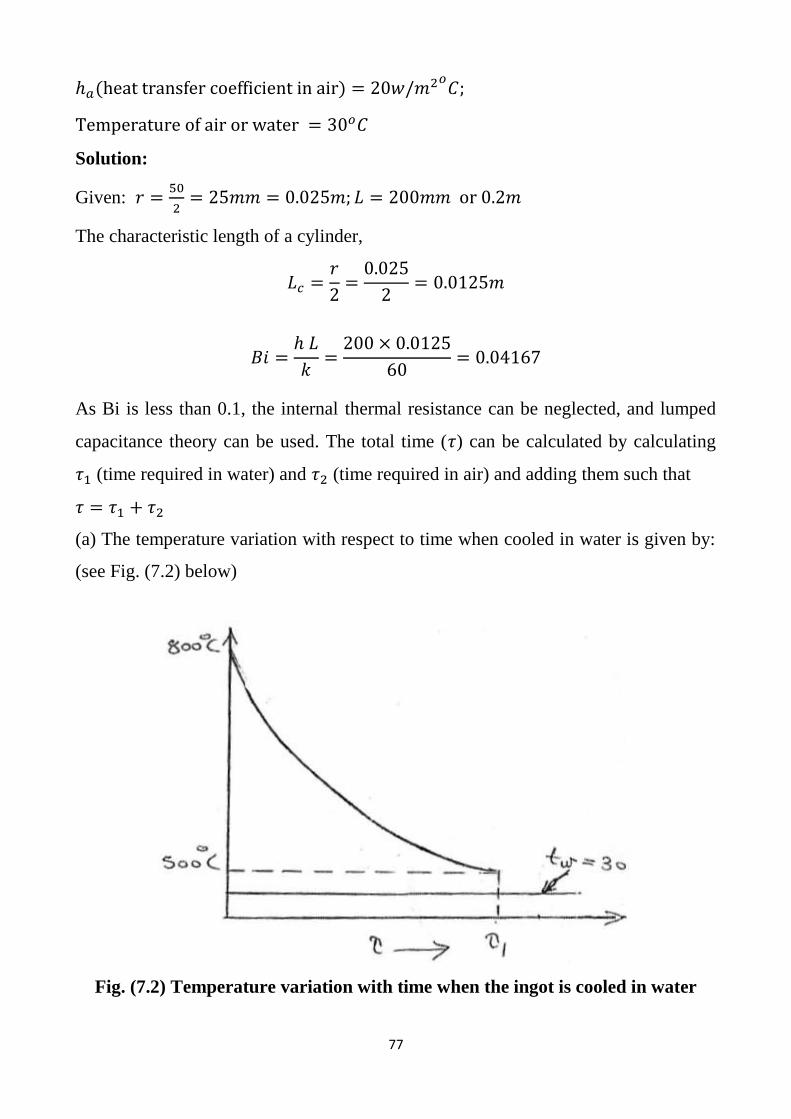
77

ℎ𝑎(heat transfer coefficient in air) = 20𝑤/𝑚2𝑜𝐶;

Temperature of air or water = 30𝑜𝐶

Solution:

Given: 𝑟 =50

2= 25𝑚𝑚 = 0.025𝑚; 𝐿 = 200𝑚𝑚 or 0.2𝑚

The characteristic length of a cylinder,

𝐿𝑐 =𝑟

2=

0.025

2= 0.0125𝑚

𝐵𝑖 =ℎ 𝐿

𝑘=

200 × 0.0125

60= 0.04167

As Bi is less than 0.1, the internal thermal resistance can be neglected, and lumped

capacitance theory can be used. The total time (𝜏) can be calculated by calculating

𝜏1 (time required in water) and 𝜏2 (time required in air) and adding them such that

𝜏 = 𝜏1 + 𝜏2

(a) The temperature variation with respect to time when cooled in water is given by:

(see Fig. (7.2) below)

Fig. (7.2) Temperature variation with time when the ingot is cooled in water

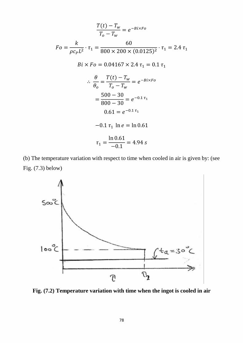
78

𝑇(𝑡) − 𝑇𝑤

𝑇𝑜 − 𝑇𝑤= 𝑒−𝐵𝑖×𝐹𝑜

𝐹𝑜 =𝑘

𝜌𝑐𝑃𝐿2⋅ 𝜏1 =

60

800 × 200 × (0.0125)2⋅ 𝜏1 = 2.4 𝜏1

𝐵𝑖 × 𝐹𝑜 = 0.04167 × 2.4 𝜏1 = 0.1 𝜏1

∴ 𝜃

𝜃𝑜=

𝑇(𝑡) − 𝑇𝑤

𝑇𝑜 − 𝑇𝑤= 𝑒−𝐵𝑖×𝐹𝑜

=500 − 30

800 − 30= 𝑒−0.1 𝜏1

0.61 = 𝑒−0.1 𝜏1

−0.1 𝜏1 ln 𝑒 = ln 0.61

𝜏1 =ln 0.61

−0.1= 4.94 𝑠

(b) The temperature variation with respect to time when cooled in air is given by: (see

Fig. (7.3) below)

Fig. (7.2) Temperature variation with time when the ingot is cooled in air

79

∴ 𝜃

𝜃𝑜=

𝑇(𝑡) − 𝑇𝑎

𝑇𝑜 − 𝑇𝑎= 𝑒−𝐵𝑖×𝐹𝑜

𝐵𝑖 =ℎ 𝐿

𝑘=

20 × 0.0125

60= 0.004167

𝐹𝑜 =𝑘

𝜌𝑐𝑃𝐿2⋅ 𝜏2 = 2.4 𝜏2

𝐵𝑖 × 𝐹𝑜 = 0.004167 × 2.4 𝜏2 = 0.01 𝜏2

𝜃

𝜃𝑜=

100 − 30

500 − 30=

70

470= 𝑒−0.01 𝜏2

0.149 = 𝑒−0.01 𝜏2

−0.01 𝜏2 ln 𝑒 = ln 0.149

∴ 𝜏2 =ln 0.149

−0.01 × 1= 190.42 𝑠

Total time (𝜏) is given by:

𝜏 = 𝜏1 + 𝜏2 = 4.94 + 190.42 = 195.36 𝑠 = 3.256 𝑚𝑖𝑛.

80

Chapter Eight

Unsolved Theoretical Questions and Further Problems in

Lumped Capacitance System

8.1 Theoretical Questions:

1. What is meant by transient heat conduction?

2. What is lumped capacity?

3. What are the assumptions for lumped capacity analysis?

4. What are Fourier and Biot numbers? What is the physical significance of these

numbers?

5. Define a semi – infinite body.

6. What is an error function? Explain its significance in a semi – infinite body in

transient state.

7. What are Heisler charts?

8. Explain the significance of Heisler charts in solving transient conduction problems.

8.2 Further Problems:

1. A copper slab (𝜌 = 9000𝑘𝑔/𝑚3, 𝑐 = 380𝐽/𝑘𝑔𝑜𝐶, 𝑘 = 370𝑤/𝑚𝑜𝐶) measuring

400𝑚𝑚 × 400𝑚𝑚 × 5𝑚𝑚 has a uniform temperature of 250𝑜𝑐. Its temperature is

suddenly lowered to 30𝑜𝐶. Calculate the time required for the plate to reach the

temperature of 90𝑜𝐶. Assume convective heat transfer coefficient as 90𝑤/𝑚2𝑜𝐶 .

𝑨𝒏𝒔. {𝟏𝟐𝟑. 𝟕𝟓 𝒔}

2. An aluminum alloy plate 0.2𝑚2 surface area (both sides), 4mm thick and at 200𝑜𝐶

is suddenly quenched into liquid oxygen which is at -183𝑜𝐶 . Find the time required

for the plate to reach the temperature of -70𝑜𝐶 .

Take: 𝜌 = 2700𝑘𝑔/𝑚3, 𝑐 = 890𝐽/𝑘𝑔𝑜𝐶, ℎ = 500𝑤/𝑚2𝑜𝐶

𝑨𝒏𝒔. {𝟐𝟑. 𝟒𝟓 𝒔 }

3. A sphere of 200mm diameter made of cast iron initially at a uniform temperature

of 400𝑜𝑐 is quenched into oil. The oil bath temperature is 40𝑜𝐶. If the temperature of

81

sphere is 100𝑜𝐶 after 5 minutes, find heat transfer coefficient on the surface of the

sphere.

Take: 𝑐𝑃 (cast iron) =0.32𝐾𝐽/𝑘𝑔𝑜𝐶; 𝜌(cast iron) =7000kg/m3


𝑨𝒏𝒔. {𝟏𝟑𝟒𝒌𝒘/𝒎𝟐𝒐𝑪}

4. An average convective heat transfer coefficient for flow of 100𝑜𝐶 air over a flat

plate is measured by observing the temperature – time history of a 30 mm thick

copper slab (𝜌 = 9000𝑘𝑔/𝑚3, 𝑐 = 0.38𝑘𝐽/𝑘𝑔𝑜𝐶, 𝑘 = 370𝑤/𝑚𝑜𝐶) exposed to

100𝑜𝐶 air. In one test run, the initial temperature of the plate was 210𝑜𝐶 and in 5

minutes the temperature decreased by 40𝑜𝐶 . Find the heat transfer coefficient for

this case. Neglect internal thermal resistance.

𝑨𝒏𝒔. {𝟕𝟕. 𝟐𝟒𝒘/𝒎𝟐𝒐𝑪}

5. A cylinder steel ingot 150mm in diameter and 400mm long passes through a heat

treatment furnace which is 6m in length. The ingot must reach a temperature of

850𝑜𝐶 before it comes out of the furnace. The furnace gas is at 1280𝑜𝐶 and ingot

initial temperature is 100𝑜𝐶. What is the maximum speed with which the ingot

should move in the furnace to attain the required temperature? The combined

radiative and convective surface heat transfer coefficient is 100𝑤/𝑚2𝑜𝐶. Take k

(steel)= 45𝑤/𝑚𝑜𝐶 and 𝛼 (thermal diffusivity) = 0.46 × 10−5𝑚2/𝑠.

𝑨𝒏𝒔. { 𝟏. 𝟔𝟏𝟗 × 𝟏𝟎−𝟑𝒎/𝒔 }

6. A hot mild steel sphere (𝑘 = 42.5𝑤/𝑚𝑜𝐶) having 12mm diameter is planned to be

cooled by an air flow at 27𝑜𝐶. The convective heat transfer coefficient is 114𝑤/

𝑚2𝑜𝐶. Determine the following:

(i) Time required to cool the sphere from 540𝑜𝐶 to 95𝑜𝐶;

(ii) Instantaneous heat transfer rate 2 minutes after the start of cooling;

(iii) Total energy transferred from the sphere during the first 2 minutes. Take mild

steel properties as (𝜌 = 7850𝑘𝑔/𝑚3, 𝑐 = 475𝑘𝐽/𝑘𝑔𝑜𝐶 , 𝛼 = 0.043𝑚2/ℎ).

𝑨𝒏𝒔. { (𝒊) 𝟐. 𝟏𝟎𝟒 𝒎𝒊𝒏; (𝒊𝒊) 𝟑. 𝟖𝟖𝟒𝒘 ; (𝒊𝒊𝒊) 𝟏𝟒𝟕𝟓. 𝟕 𝑱}

82

7. The heat transfer coefficients for the flow of 30𝑜𝐶 air over a 12.5mm diameter

sphere are measured from observing the temperature – time history of a copper ball

of the same dimensions. The temperature of the copper ball (𝜌 = 8930𝑘𝑔/𝑚3; 𝑐 =

0.375𝑘𝐽/𝑘𝑔𝑜𝐶) was measured by two thermocouples, one located at the center and

the other near the surface. Both thermocouples registered within the accuracy of the

recording instruments the same temperature at the given instant, on one test run, the

initial temperature of the ball was 70𝑜𝐶 and in 1.15 minutes the temperature

decreased by 7𝑜𝐶. Calculate the convective heat transfer coefficient for this case.

Ans. {𝟏𝟗𝟒. 𝟓 𝒘/𝒎𝟐𝒐𝑪}

8. The temperature of an air stream flowing with a velocity of 3 m/s is measured by a

copper – constantan thermocouple which may be approximated as a sphere 3mm in

diameter. Initially the junction and air are at a temperature of 25𝑜𝐶. The air

temperature suddenly changes to and is maintained at 200𝑜𝐶.

i) Determine the time required for the thermocouple to indicate a temperature of

150𝑜𝐶. Also determine the thermal time constant and temperature indicated by the

thermocouple at that instant;

ii) Discuss the suitability of this thermocouple to measure unsteady state temperature

of a fluid when the temperature variation in the fluid has a time period of 3 seconds.

The thermocouple junction properties are:

Density = 8685𝑘𝑔/𝑚3 ; specific heat 𝑐 = 383 𝑗/𝑘𝑔𝑜𝐶 ; thermal conductivity

(thermocouple) 𝑘 = 29𝑤/𝑚𝑜𝐶 and convective coefficient ℎ = 150𝑤/𝑚2𝑜𝐶 .

Ans. {𝟏𝟑. 𝟖𝟗 𝒔; 𝟏𝟏. 𝟎𝟗 𝒔 ; 𝟏𝟓𝟓. 𝟔𝟑𝒐𝑪}

9. A 50 mm thick large steel plate (𝑘 = 42.5𝑤/𝑚𝑜𝐶, 𝛼 = 0.043 𝑚2/ℎ), initially at

425𝑜𝐶 is suddenly exposed on both sides to an environment with convective heat

transfer coefficient 285𝑤/𝑚2𝑜𝐶 and temperature 65𝑜𝐶 . Determine the center line

temperature and temperature inside the plate 12.5mm from the mid-plane after 3

minutes.

10. A long cylindrical bar (𝑘 = 17.5𝑤/𝑚𝑜𝐶, 𝛼 = 0.0185 𝑚2/ℎ) of radius 75mm

comes out of oven at 815𝑜𝐶 throughout and is cooled by quenching it in a large bath

83

of 38𝑜𝐶 coolant. The surface coefficient of heat transfer between the bar surface and

the coolant is 175𝑤/𝑚2𝑜𝐶. Determine:

(i) The time taken by the shaft to reach 116𝑜𝐶 ;

(ii) The surface temperature of the shaft when its center temperature is 116𝑜𝐶. Also

calculate the temperature gradient at the outside surface at the same instant of time.

Ans. {(𝒊) 𝟐𝟏𝟎𝟐𝒔; (𝒊𝒊) 𝟗𝟐. 𝟔𝒐𝑪; 𝟓𝟒𝟔𝒐𝑪/𝒎}

11. A concrete highway may reach a temperature of 55𝑜𝐶 on a hot summer's day.

Suppose that a stream of water is directed on the highway so that the surface

temperature is suddenly lowered to 35𝑜𝐶. How long will it take to cool the concrete

to 45𝑜𝐶 at a depth of 50mm from the surface?

For concrete take 𝛼 (thermal diffusivity) = 1.77 × 10−3𝑚2/ℎ

Ans. {𝟏. 𝟓𝟏 𝒉}

12. It is proposed to bury water pipes underground in wet soil which is initially at

4.5𝑜𝐶. The temperature of the surface of soil suddenly drops to −5𝑜𝐶 and remains at

this value for 10 hours. Determine the minimum depth at which the pipes be laid if

the surrounding soil temperature is to remain above 0𝑜𝐶 (without water getting

frozen). Assume the soil as semi – infinite soild.

For wet soil take 𝛼 (thermal diffusivity) = 2.78 × 10−3𝑚2/ℎ

Ans. {𝟎. 𝟏𝟔𝟕𝒎}

13. A 50 mm thick mild steel plate (𝛼 = 1.25 × 10−5𝑚2/𝑠) is initially at a

temperature of 40𝑜𝐶. It is suddenly exposed on one side to a fluid which causes the

surface temperature to increase to and remain at 90𝑜𝐶. Determine:

(i) The maximum time that the slab be treated as a semi – infinite body;

(ii) The temperature as the center of the slab one minute after the change in surface

temperature.

Ans. {(𝒊) 𝟐𝟎𝟎𝒔 ; (𝒊𝒊) 𝟔𝟔𝒐𝑪}

14. The initial uniform temperature of a thick concrete wall (𝛼 = 1.58 × 10−3𝑚2/ℎ;

𝑘 = 0.937𝑤/𝑚𝑜𝐶) of a jet engine test cell is 21𝑜𝐶. The surface temperature of the

84

wall suddenly rises to 315𝑜𝐶 when the combination of exhaust gases from the

turbojet and spray of cooling water occurs. Determine:

(i) The temperature at a point 75 mm from the surface after 7.5 hours;

(ii) The instantaneous heat flow rate at the specified plane and at the surface itself at

the instant mentioned at (i).

Use the solution for semi – infinite solid.

Ans. {(𝒊) 𝟐𝟎𝟔𝒐𝑪; (𝒊𝒊) − 𝟏𝟐𝟔𝟓. 𝟔𝒘/𝒎𝟐; −𝟏𝟒𝟐𝟓𝒘/𝒎𝟐}

15. The initial uniform temperature of a large mass of material (𝛼 = 0.41 𝑚2/ℎ) is

120𝑜𝐶. The surface of the material is suddenly exposed to and held permanently at

5𝑜𝐶. Calculate the time required for the temperature gradient at the surface to reach

350𝑜𝐶/𝑚.

Ans. {𝟐𝟎𝟔𝒔}

16. A motor car of mass 1500 kg travelling at 80 km/h is brought to rest within a

period of 5 seconds when brakes are applied. The braking system consists of 4 brakes

with each brake band of 350 𝑐𝑚2 area; these press against steel drum of equivalent

area. The brake lining and the drum surfaces (𝑘 = 55𝑤/𝑚𝑜𝐶, 𝛼 = 1.24 ×

10−5𝑚2/𝑠) are at the same temperature and the heat generated during the stoppage

action dissipates by flowing across drums. If the drum surface is treated as semi –

infinite plate, calculate the maximum temperature rise.

Ans. {𝟏𝟑𝟒. 𝟏𝟏𝒐𝑪}

17. During periodic heating and cooling of a thick brick wall, the wall temperature

varies sinusoidally. The surface temperature ranges from 25𝑜𝐶 to 75𝑜𝐶 during a

period of 24 hours. Determine the time lag of the temperature wave corresponding to

a point located at 250 mm from the wall surface. The properties of the wall material

are: (𝜌 = 1620𝑘𝑔/𝑚3, 𝑐 = 450𝐽/𝑘𝑔𝑜𝐶, 𝑘 = 0.62𝑤/𝑚𝑜𝐶).

Ans. {𝟔. 𝟐𝟒 𝒉}

18. A single cylinder (𝛼 = 0.042 𝑚2/ℎ from cylinder material) two – stroke I.C.

engine operates at 1500 𝑟. 𝑝. 𝑚. Calculate the depth where the temperature wave due

to variation of cylinder temperature is damped to 1% of its surface value.

85

Ans. {𝟏. 𝟕𝟕𝟓 𝒎𝒎}

19. The temperature distribution across a large concrete slab (𝑘 = 1.2𝑤/𝑚𝑜𝐶, 𝛼 =

1.77 × 10−3𝑚2/ℎ) 500 mm thick heated from one side as measured by

thermocouples approximates to the relation: 𝑡 = 60 − 50𝑥 + 12𝑥2 + 20𝑥3 − 15𝑥4

where 𝑡 is in o𝐶 and 𝑥 is in meters. Considering an area of 5𝑚2, compute the

following:

(i) The heat entering and leaving the slab in unit time;

(ii) The heat energy stored in unit time;

(iii) The rate of temperature change at both sides of the slab; and

(iv) The point where the rate of heating or cooling is maximum.

Ans. {(𝒊) 𝟑𝟎𝟎𝒘, 𝟏𝟖𝟑 𝒘; (𝒊𝒊) 𝟏𝟏𝟕𝒘; (𝒊𝒊𝒊) 𝟒𝟐. 𝟒𝟖 × 𝟏𝟎−𝟑𝒐𝒄/𝒉, 𝟔𝟗. 𝟎𝟑 ×

𝟏𝟎−𝟑𝒐𝒄/𝒉; (𝒊𝒗) 𝟎. 𝟑𝟑𝒎}

86

References

1. M. David Burghardt and James A. Harbach, "Engineering Thermodynamics",

Fourth Edition, Harper Collins College Publishers, (1993).

2. R. K. Rajput, "Engineering Thermodynamics", Third Edition, SI units version,

Laxmi Publications LTD, New Delhi, India (2007).

3. Michael J. Moran and Howard N. Shapiro, "Fundamentals of Engineering

Thermodynamics", Fifth Edition, SI units, John Wiley and Sons, Inc., England,

(2006).

4. Theodore L. Bergman and et al., "Fundamentals of Heat and Mass Transfer",

Seventh Edition, John Wiley and Sons, Inc., England, (2011).

5. Eastop and McConkey, "Applied Thermodynamics for Engineering

Technologists", Fifth Edition, Longman Group UK Limited, London, (1993).

6. Osama Mohammed Elmardi, "Solution of Problems in Heat and Mass Transfer", in

Arabic language, www.ektab.com, December (2015).

7. Osama Mohammed Elmardi, "Lecture Notes on Thermodynamics I", in Arabic

language, Mechanical Engineering Department, Faculty of Engineering and

Technology, Nile Valley University, (1998).

8. Osama Mohammed Elmardi, "Lecture Notes on Thermodynamics II", in Arabic

language, Mechanical Engineering Department, Faculty of Engineering and

Technology, Nile Valley University, (2000).

9. R.K. Rajput, "Heat and Mass Transfer", SI units, S. Chand and Company LTD,

New Delhi, (2003).

10. Welty J. R., "Fundamentals of Momentum, Heat and Mass Transfer", 3rd edition,

John Wiley, (1984).

11. Croft D.R. and Lilley D.G., "Heat Transfer Calculations using Finite Difference

Equations", Pavic Publications, (1986).

12. Incropera F. P. and De Witt D.P., "Fundamentals of Heat and Mass Transfer", 3rd

edition, John Wiley, (1990).

http://www.ektab.com/

87

13. Rogers G.F.C. and Mayhew Y.R., "Thermodynamics and Transport Properties of

Fluids", 4th edition, Basil Blackwell, (1987).

14. Eckert E.R. and Drake R.M., "Analysis of Heat and Mass Transfer", Taylor and

Francis, (1971).

15. Kern D.Q., "Process Heat Transfer", McGraw – Hill, (1950).

16. M. J. C. Van Gemert, "Theoretical analysis of the lumped capacitance method in

dielectric time domain spectroscopy", Journal of Advances in Molecular Relaxation

Processes, Received 12 November (1973), Available online 3 October (2002).

17. Faghri A., Zhang Y., and Howell J. R., "Advanced Heat and Mass Transfer",

Global Digital Press, Columbia, (2010).

18. M. Bahrami, "Transient Conduction Heat Transfer", ENSC 388 (F09).

19. Professor M. Zenouzi, "Transient Response Characteristics and Lumped System

Analysis of Geometrically Similar Objects" October 1, (2009).

20. R. Shankar Subramanian, ""Unsteady Heat Transfer: Lumped Thermal Capacity

Model", Department of Chemical and Biomolecular Engineering, Clarkson

University.

21. P. K. Nag, "Heat and Mass Transfer", Second Edition, Tata McGraw Hill

Publishing Company Limited, New Delhi, (2007).

22. Yunus A. Cengel, and Afshin J. Ghajar, "Heat and Mass Transfer: Fundamentals

and Applications", Fourth Edition, McGraw Hill, (2011).

23. M. Thirumaleshwar, "Fundamentals of Heat and Mass Transfer", Second

Impression, Published by Dorling Kindersley, India, (2009).

24. World Heritage Encyclopedia, "Lumped System Analysis", Published by World

Heritage Encyclopedia.

25. Balaram Kundu, Pramod A. Wankhade, "Analytical Temperature Distribution on

a Turbine Blade Subjected to Combined Convection and Radiation Environment",

Journal of Thermal Engineering, Vol. 2, No. 1, January (2016), PP. (524 – 528).

26. Sepideh Sayar, "Heat Transfer During Melting and Solidification in

Heterogeneous Materials", Thesis in Master of Science in Mechanical Engineering,

Blacksburg, Virginia, December (2000).

88

27. M. Khosravy, "Transient Conduction", Islamic Azad University, Karaj Branch.

28. Lienhard, John H., "A Heat Transfer Textbook", Cambridge, Massachusetts,

Phlogiston Press, ISBN 978 – 0 – 9713835 – 3 – 1, (2008).

29. Welty James R. and Wicks Charles E., "Fundamentals of momentum, heat and

mass transfer", 2nd edition, New York, Wiley, ISBN 978 – 0 – 471 – 93354 – 0,

(1976).

30. Paul A. Tipler and Gene Mosca, "Physics for Scientists and Engineers", 6 th

edition, New York, Worth Publishers, ISBN 1 – 4292 – 0132 – 0, (2008), PP. (666 –

670).

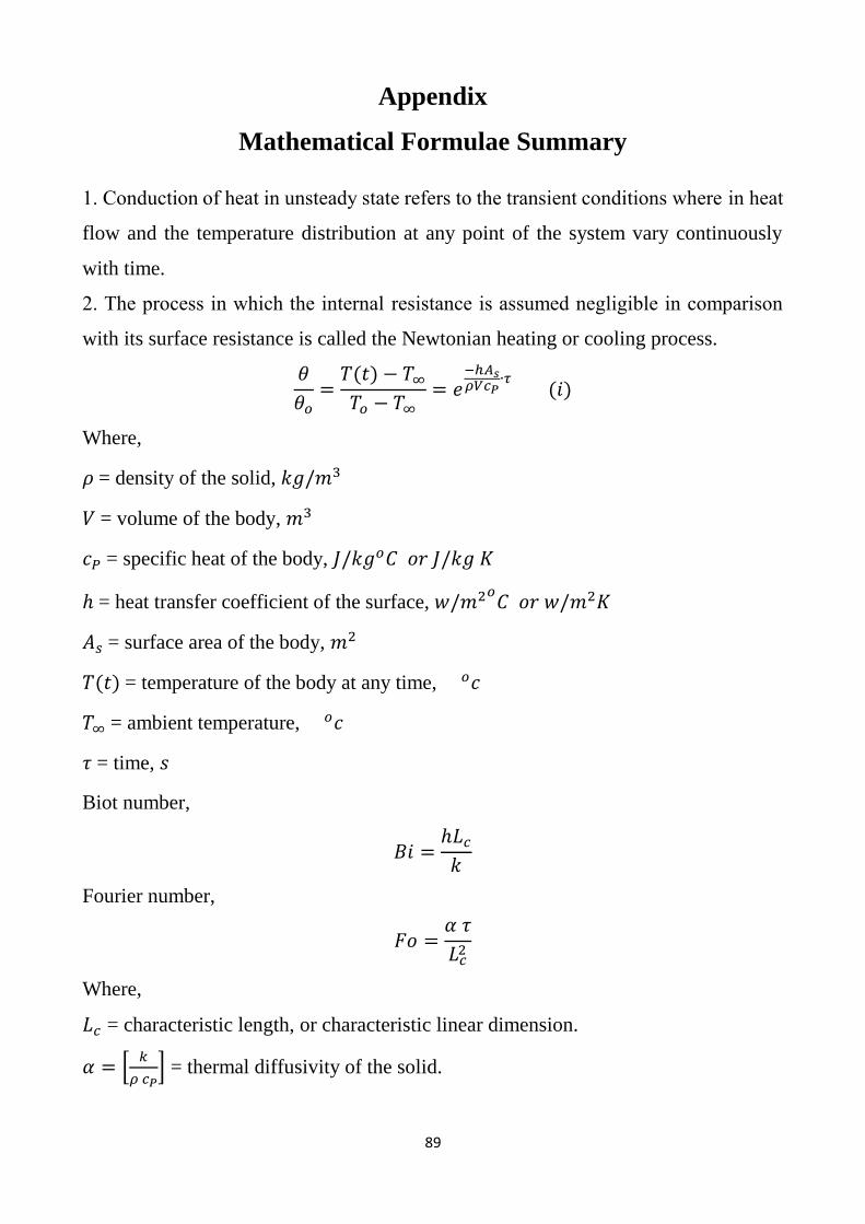
89

Appendix

Mathematical Formulae Summary

1. Conduction of heat in unsteady state refers to the transient conditions where in heat

flow and the temperature distribution at any point of the system vary continuously

with time.

2. The process in which the internal resistance is assumed negligible in comparison

with its surface resistance is called the Newtonian heating or cooling process.

𝜃

𝜃𝑜=

𝑇(𝑡) − 𝑇∞

𝑇𝑜 − 𝑇∞= 𝑒

−ℎ𝐴𝑠𝜌𝑉𝑐𝑃

∙𝜏 (𝑖)

Where,

𝜌 = density of the solid, 𝑘𝑔/𝑚3

𝑉 = volume of the body, 𝑚3

𝑐𝑃 = specific heat of the body, 𝐽/𝑘𝑔𝑜𝐶 𝑜𝑟 𝐽/𝑘𝑔 𝐾

ℎ = heat transfer coefficient of the surface, 𝑤/𝑚2𝑜𝐶 𝑜𝑟 𝑤/𝑚2𝐾

𝐴𝑠 = surface area of the body, 𝑚2

𝑇(𝑡) = temperature of the body at any time, 𝑜𝑐

𝑇∞ = ambient temperature, 𝑜𝑐

𝜏 = time, 𝑠

Biot number,


𝑘

Fourier number,

𝐹𝑜 =𝛼 𝜏

𝐿𝑐2

Where,

𝐿𝑐 = characteristic length, or characteristic linear dimension.

𝛼 = [𝑘

𝜌 𝑐𝑃] = thermal diffusivity of the solid.

90

𝜃

𝜃𝑜=

𝑇(𝑡) − 𝑇∞

𝑇𝑜 − 𝑇∞= 𝑒−𝐵𝑖× 𝐹𝑜 (𝑖𝑖)

Instantaneous heat flow rate:

𝑞′(𝜏) = −ℎ𝐴𝑠(𝑇𝑜 − 𝑇∞)𝑒−𝐵𝑖×𝐹𝑜 (𝑖𝑖𝑖)

Total or cumulative heat transfer:

𝑄(𝑡) = 𝜌𝑉 𝑐𝑃(𝑇𝑜 − 𝑇∞)[𝑒−𝐵𝑖×𝐹𝑜 − 1] (𝑖𝑣)

3. Time constant and response of temperature measuring instruments:

The quantity 𝜌𝑉 𝑐𝑃

ℎ𝐴𝑠 is called time constant (𝜏∗).

𝜃

𝜃𝑜=

𝑇(𝑡) − 𝑇∞

𝑇𝑜 − 𝑇∞= 𝑒−(𝜏/𝜏∗)

The time required by a thermocouple to reach its 63.2% of the value of the initial

temperature difference is called its sensitivity.

4. Transient heat conduction in semi – infinite solids (ℎ or 𝐵𝑖 → ∞): The temperature

distribution at any time 𝜏 at a plane parallel to and at a distance 𝑥 from the surface

is given by:

𝑇(𝑡) − 𝑇∞


𝑥

2√𝛼 𝜏] (𝑖)

Where 𝑒𝑟𝑓 [𝑥

2√𝛼 𝜏] is known as "Gaussian error function".

The instantaneous heat flow rate at a given x – location within the semi – infinite

body at a specified time is given by:

𝑄𝑖 = −𝑘𝐴(𝑇𝑜 − 𝑇∞)𝑒[−𝑥2/4𝛼𝜏]

√𝜋 𝛼 𝜏 (𝑖𝑖)

The heat flow rate at the surface (𝑥 = 0) is given by:

𝑄𝑠𝑢𝑟𝑓𝑎𝑐𝑒 == −𝑘𝐴(𝑇𝑜 − 𝑇∞)

√𝜋 𝛼 𝜏 (𝑖𝑖𝑖)

The heat flow rate 𝑄(𝑡) is given by:

91

𝑄(𝑡) = −1.13𝑘𝐴(𝑇𝑜 − 𝑇∞)√𝜏

𝛼 (𝑖𝑣)

92

Author

Osama Mohammed Elmardi Suleiman was born in Atbara,

Sudan in 1966. He received his diploma degree in mechanical

engineering from Mechanical Engineering College, Atbara,

Sudan in 1990. He also received a bachelor degree in

mechanical engineering from Sudan University of Science and

Technology – Faculty of Engineering in 1998, and a master

degree in solid mechanics from Nile Valley University (Atbara, Sudan) in 2003. He

contributed in teaching some subjects in other universities such as Red Sea

University (Port Sudan, Sudan), Kordofan University (Obayied, Sudan), Sudan

University of Science and Technology (Khartoum, Sudan) and Blue Nile University

(Damazin, Sudan). In addition, he supervised more than hundred and fifty under

graduate studies in diploma and B.Sc. levels and about fifteen master theses. He is

currently an assistant professor in department of mechanical engineering, Faculty of

Engineering and Technology, Nile Valley University. His research interest and

favorite subjects include structural mechanics, applied mechanics, control

engineering and instrumentation, computer aided design, design of mechanical

elements, fluid mechanics and dynamics, heat and mass transfer and hydraulic

machinery. He also works as a consultant and technical manager of Al – Kamali

workshops group for small industries in Atbara old and new industrial areas.

Documents

Solution of Problems in Heat Transfer Transient Conduction