Embed Size (px)
Citation preview

Topic 14
Sections 9.3.1, 9.3.2, 9.3.3, 9.5.3, 8.2.4
9.6,9.7,9.8,9.11
Contents: •••••••••••
Mode superposition analysis in nonlinear dynamics
Substructuring in nonlinear dynamics, a schematicexample of a building on a flexible foundation
Study of analyses to demonstrate characteristics ofprocedures for nonlinear dynamic solutions
Example analysis: Wave propagation in a rod
Example analysis: Dynamic response of a three degree offreedom system using the central difference method
Example analysis: Ten-story tapered tower subjected toblast loading
Example analysis: Simple pendulum undergoing largedisplacements
Example analysis: Pipe whip solution
Example analysis: Control rod drive housing with lowersupport
Example analysis: Spherical cap under uniform pressureloading
Example analysis: Solution of fluid-structure interactionproblem
Solution ofNonlinearDynamicResponse-Part II
Textbook:
Examples:
14-2 Nonlinear Dynamic Response - Part II
References: The use of the nonlinear dynamic analysis techniques is described withexample solutions in
Bathe, K. J., "Finite Element Formulation, Modeling and Solution ofNonlinear Dynamic Problems," Chapter in Numerical Methodsjor Partial Differential Equations, (Parter, S. V., ed.), Academic Press, 1979.
Bathe, K. J., and S. Gracewski, "On Nonlinear Dynamic Analysis UsingSubstructuring and Mode Superposition," Computers & Structures, 13,699-707,1981.
Ishizaki, T., and K. J. Bathe, "On Finite Element Large Displacementand Elastic-Plastic Dynamic Analysis of Shell Structures," Computers& Structures, 12, 309-318, 1980.

TH E S OLV\T ION 0 F
TH E ']) 'YNAM Ie EQUlLJ B-
~IUH ElluATIONS CAN
'5£ ACHI£VE~ US1I'Jb
'DIR=,-T "I.NTE{;RATJON
Me-PtobS,
_ E,>£PL\C tT lNTE. 5R.
S~B'STR lACTu'R 11\15
w~ I)lSCUSS i~ESE l~H'
NIQuES ~'R'EFL'I I~ \t\\S
LEe.n,fi<.E
WAVE t'RO?A6A
IN A 1"01>
\Ex.,- 1':ESl'ONSE OF A
3 :).O.F. S'tS"TEP-1
\
E.)(,S ANAl.'1S1S OF
TE N ~To"R'I
IA'PE:'KEb TOWER
\
EX,4- AN!\L"ISI'i> O~
1>E N b\.A LtA M
\
EXS P\?E wlil?
'RES"PONS,c SOUA110N
Topic Fourteen 14-3
. A""AL't~IS OF CR.b
1-1011\'>11\1&
SOL-I.tTION OF "RE::C;?ONS~
OF S'PHE~llAL CAP
• At-IAL'ISI<;' OF FLU,J)
ST'RlA(.TI.t'RE III.1T~AC.:noN
"P1<:OJ3.LE t1 ('t:>1 i"E. lEST)
THE 1:>E:TAIL.'S, Of'
nlESE "?'R~~LEl'-\
S,bLuTICNc:. "~E
61\1E III 1 N THE
"f~'PE'RS SE.EI
STUb,! oLAlbE
Markerboard14-1

14-4 Nonlinear Dynamic Response - Part II
Transparency14-1
Mode superposition:
• The modes of vibration change due tothe nonlinearities, however we canemploy the modes at a particular timeas basis vectors (generalizeddisplacements) to express theresponse.
• This method is effective when, innonlinear analysis,
- the response lies in only a fewvibration modes (displacementpatterns)
- the system has only localnonlinearities
Transparency14-2
The governing equations in implicit timeintegration are (assuming no dampingmatrix)M HLltO(k) + TK ~U(k) = HLltR _ HLltF(k-1)- - -
Let now T = 0, hence the method ofsolution corresponds to the initial stressmethod.
Using

The modal transformation gives
H.:1tX(k) + 0 2 ax(k) = <I>T (H.:1tR _ H.:1tF(k-1»)
Topic Fourteen 14-5
Transparency14-3
where
n2 = [W~"W~]<I> = ~r ... ~s]
.equations cannot be solvedindividually over the timespanCoupling!
Typical problem:
~~========:::::::D!I~
Pipe whip: Elastic-plastic pipeElastic-plastic stop
• Nonlinearities in pipe and stop. Butthe displacements are reasonably wellcontained in a few modes of thelinear (initial) system.
Transparency14-4

1~ Nonlinear Dynamic Response - Part II
Transparency14-5
Substructuring
• Procedure is used with implicit timeintegration. All linear degrees offreedom can be condensed out priorto the incremental solution.
• Used for local nonlinearities:Contact problemsNonlinear support problems
p-0
_0
oSlip
Transparency14-6
Example:
Ten storybuilding Finite element
model
• -"master" node
• - substructureinternal node
Substructuremodel

/t A
K
master dot
substructureinternal dot
master dot
substructureinternal dot
master dot
Topic Fourteen 14-7
Transparency14-7
Here
tA
( 4) tK = K + Llt2 M + Knonlinear
~ toil mass~1I nonlinear stiffnessI matrix effectsall linearelement contributions
A tK + K nonlinear- -
Transparency14-8

14-8 Nonlinear Dynamic Response - Part II
Transparency14-9
Transparency14-10
After condensing out all substructureinternal degrees of freedom, we obtaina smaller system of equations:
~entries from condensed
1_.........7rUbstruclures
master dof
Major steps in solution:
• Prior to step-by-step solution,establish Bfor all mass and constantstiffness contributions. Staticallycondense out internal substructuredegrees of freedom to obtain Be.We note that
t A A t.!Sc = .!SC + .!Snonlinear
condensed i. all nonlinear effects7 A 4
from K= K+ .lt2 M
alllinearJ "-total mass matrixelement contributions

• For each time step solution (and eachequilibrium iteration):
- Update condensed matrix, Ke, fornonlinearities.
- Establish complete load vector for alldegrees of freedom and condense outsubstructure internal degrees of freedom.
- Solve for master dof displacements,velocities, accelerations and calculate allsubstructure dof disp., veL, ace.
The substructure internal nodal disp., veL,ace. are needed to calculate the completeload vector (corresponding to all dof).
Solution procedure for each time step(and iteration):
tu t+4tU-, -,tU' t+4t(j-, • t+4tRA _ t+4tRA _ t+41U _ -,.. _ _c _c t+4tU"tu
Topic Fourteen 14-9
Transparency14-11
Transparency14-12
substructuredegrees offreedomcondensedout
usingcondensedeffectivestiffnessmatrix tKe

14-10 Nonlinear Dynamic Response - Part II
Example: Wave propagation in a rodTransparency
14-13
R
Uniform, freely floating rod
/
R
1000 N+------
L = 1.0 mA = 0.01 m'Z.p = 1000 kg/m3
E = 2.0 x 10⁹ Pa
time
Transparency14-14
Consider the compressive force at apoint at the center of the rod:
-.B-1' .5 'I' .5 'I
t* = time for stress waveto travel throughthe rod1000 N
Compressiveforce
IA
The exact solution for the force atpoint A is shown below.
1....-_--+-__\--_-+-_--+__ time1/2 t* t* % t* 2 t*

We now use a finite element mesh often 2-node truss elements to obtainthe compressive force at point A.
All elements uniformly spaced
Topic Fourteen 14-11
Transparency14-15
R • •
Central difference method:
• The critical time step for this problem is
Llt = L Ic = t* ( 1 )cr e number of elements
Llt > Lltcr will produce an unstablesolution
• We need to use the inital conditionsas follows:
aMOO~=OR
~0·· _ °HUj -
mjj
Transparency14-16

14-12 Nonlinear Dynamic Response - Part II
exact
/
1500
• Using a time step equal to atcr• we obtainthe correct result: • For this special
case the exactsolution is obtained
Finite elements
~100QCompressiveforce (N) 500
Transparency14-17
t*
-500
Transparency14-18
• Using a time step equal to ! atcr , thesolution is stable, but highlyinaccurate.
Finite elements1500
1000Compressiveforce (N) 500..
-500.
time

1500
1000Compressiveforce (N) 500
Now consider the use of thetrapezoidal rule:
• A stable solution is obtained withany choice of at.
• Either a consistent or lumpedmass matrix may be used. Weemploy a lumped mass matrix inthis analysis.
Trapezoidal rule, dt = dterlcDM' .i.nitialconditions computed using MOU = OR.
- The solution is inaccurate.Finite element solution,
/"10 element meshAA/
AA exact solution
A A/A
Topic Fourteen 14-13
Transparency14-19
Transparency14-20
-500
t* 2t* timeAA

14-14 Nonlinear Dynamic Response - Part 11
1500
1000Compressiveforce (N)
500
Transparency14-21
Trapezoidal rule, dt = dtcrlcDM' zeroinitial conditions.
- Almost same solution is obtained.Finite element solution,
/ 10 element mesh
(!) (!) (!) exact solution(!) '" ~ f
(!)(!)(!
(!)(!)
Transparency14-22
t*
-500
Trapezoidal rule, dt = 2dtcrlcDM- The solution is stable, althoughinaccurate.
(!)2t* time(!)
1500Finite element solution,/10 element mesh
.t> at = 2atcrlcDM1000
Compressiveforce (N)
500
o ....t>
-500
t*
.t>exact solution~
I!:>
2t* time
Topic Fourteen 14-15
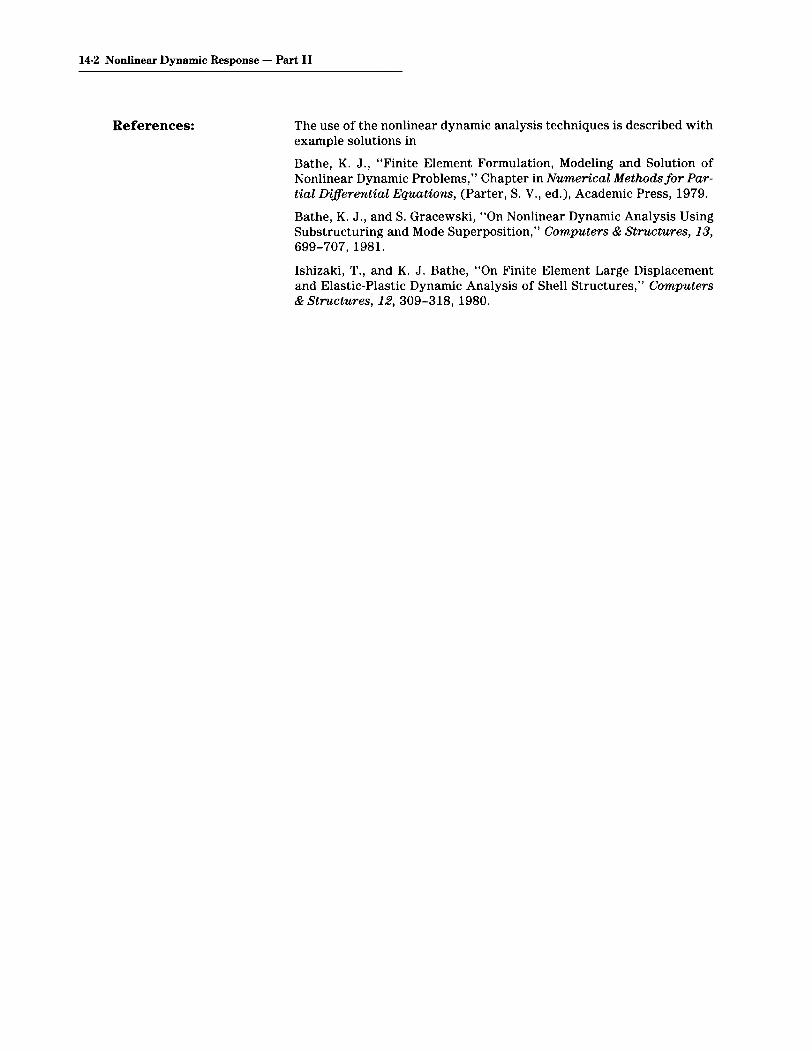
Trapezoidal rule, at = ! atcrlCDMTransparency
14-23
~
~
~<b.
t* ~~ 2t* time~
Finite element solution,er10 element mesh
~ / exact solution~~ Ao.~~ ~~ ~ ~ ~ ~~
~ ~ ~
<~
Ol~",¢ll-~L~-L_--+-__--I._~....... _
1500
1000Compressiveforce (N) 500
-500
The same phenomena are observed whena mesh of one hundred 2-node trusselements is employed.- Here ~tcr = t*/100 exact solution; finite
Finite element element solution,solution, .::It = ! .::lte., .::It = .::ltc., central
1500 central diffefrJrwenMCMeWtMfWrM-.d~iff/erence methodmethod
1000
Compressiveforce (N) 500
Transparency14·24
O+-----J.:L---+---..JH-lMIlIAAi'\r---t*
-50

14-16 Nonlinear Dynamic Response - Part II
Transparency14-25
Transparency14-26
Trapezoidal rule, at = atcrlCDM
Finite element solution, 100 element mesh
1500 /
O,+-----"'-L-----t------'"t-++t-tt1Ht----time
-50
Now consider a two-dimensional modelof the rod: tz
1 0 element 5 L- y. m./>/ .
For this mesh, atcr =P t*/(10 elements)because the element width is less thanthe element length.

If At = t*/(10 elements) is used, the solutiondiverges
-In element 5,
IT 1>- (1000 N)zz 0.01 m2
at t = 1.9 t*
Example: Dynamic response of threedegree-of-freedom systemusing central difference method
Topic Fourteen 14-17
Transparency14-27
Transparency14-28
kL = 1 Ibf/ftm = 1 slug
°X1 = °X2 = °X3 = 0
°*1 = 0.555 ft/sec°*2 = 1.000 ft/sec°*3 = 1.247 ft/sec
FomeL{:0.95
Displacement Ix2 - x3 1
(~tcrit)linear = 1.11 sec(~terit)nonlinear = 0.14 sec

14-18 Nonlinear Dynamic Response - Part II
Transparency14-29
Results: Response of right mass
3
D' 2ISp.
(ft) 1
X1 0 HJ--:-':.-----i~:---___='::n--:--~-
t(sec)-1
-2
-3.: .:1t = 0.05 sec0: .:1t = 0.15 sec
Response of center mass:Transparency
14-30
.:1 =0.05 sec.
.:1 = 0.15 sec..:O'
2Disp.(ft) 1
X2 0 1--If....L-- ~-----J~--....I...--
t(sec)-1
-2

Response of left mass:
Disp.(ft)
X320'
~\,\:>,
.... 0--
t(sec)
Topic Fourteen 14-19
Transparency14-31
.: d=0.05 sec.0: d=0.15 sec.
Force (Ibf) in center truss:
TIME dt=0.05 dt=0.159.0 -0.666 -0.700
12.0 -0.804 -0.87715.0 0.504 0.50318.0 0.648 -0.10021.0 -0.132 -0.05924.0 -0.922 0.550
Transparency14-32

14-20 Nonlinear Dynamic Response - Part II
Transparency14-33
Example: 10 story tapered tower
3.2 m--1~
Pressureinducedbyblast
Applied load (blast):
32 m
Girder properties:E=2.07x 10¹¹ Pav=0.3A=0.01 m2
As =0.009 m2
1=8.33x 10⁻⁵ m4
p = 7800 kg/m3
Transparency14-34 2000
Forceperunitlength(N/m)
1000
o+---+-----+---+--~---o 50 100 150 200
time (milliseconds)

Purpose of analysis:
• Determine displacements,velocities at top of tower.
• Determine moments at base oftower.
We use the trapezoidal rule and alumped mass matrix in the followinganalysis.
We must make two decisions:
• Choose mesh (specifically thenumber of elements employed).
• Choose time step ~t.
These two choices are closely related:
The mesh and time step to be useddepend on the loading applied.
Topic Fourteen 14·21
Transparency14-35
Transparency14-36

14-22 Nonlinear Dynamic Response - Part II
Transparency14-37
Transparency14-38
Some observations:
• The choice of mesh determinesthe highest natural frequency (andcorresponding mode shape) that isaccurately represented in the finiteelement analysis.
• The choice of time step determines the highest frequency ofthe finite element mesh in whichthe response is accurately integrated during the time integration.
• Hence, it is most effective tochoose the mesh and time stepsuch that the highest frequencyaccurately "integrated" is equal tothe highest frequency accuratelyrepresented by the mesh.
• The applied loading can be represented as a Fourier series whichdisplays the important frequenciesto be accurately represented bythe mesh.

Force perunit length(N/m)
Consider the Fourier representation ofthe load function:
f(t) = ~o +I (ancos(2'ITfnt) +bnsin(2'ITfnt»n=1
Including terms up to
case 1: fn= 17 Hz
case 2: fn= 30 Hz
The loading function is represented asshown next.
Fourier approximation including termsup to 17 Hz:
/APPlied load
/FOUrier approximation
o 100 200time (milliseconds)
Thpic Fourteen 14-23
Transparency14-39
Transparency14-40

14-24 Nonlinear Dynamic Response - Part II
Transparency14-41
Transparency14-42
Fourier approximation including termsup to 30 Hz:
2000Force perunit length(N/m)
1000
100 200time (milliseconds)
• We choose a 30 element mesh,a 60 element mesh and a 120element mesh. All elements are2-node Hermitian beam elements.
30 elements 60 elements 120 elements

Thpic Fourteen 14-25
Determine "accurate" natural frequen- .cies represented by 30 element mesh:
From eigenvalue solutions of the 30and 60 element meshes, we find
Transparency14-43
rate
curate
mode natural frequencies (Hz)number 30 element mesh 60 element mesh
1 1.914 1.9142 4.815 4.828 accu3 8.416 8.480
14 12.38 12.585 16.79 17.276 21.45 22.47
17 26.18 28.088 30.56 29.80
inac
Calculate time step:
Tco = 117 Hz = .059 sec
~t= 21 Tco = .003 sec
• A smaller time step would accurately"integrate" frequencies, which are notaccurately represented by the mesh.
• A larger time time step would notaccurately "integrate" all frequencieswhich are accurately represented bythe mesh.
Transparency14-44

14-26 Nonlinear Dynamic Response - Part II
Transparency14-45
Determine "accurate" natural frequencies represented by 60 element mesh:
From eigenvalue solutions of the 60and 120 element meshes, we find
rate
ate
mode natural frequencies (Hz)number 60 element mesh 120 element mesh
5 17.27 17.286 22.47 22.49 accur
7 28.08 28.148 29.80 29.759 32.73 33.85
10 33.73 35.0611 36.30 38.96 inaccu
Calculate time step:Transparency
14-46 Teo = 31 Hz= .033 sec
Llt == 2~ Teo = .0017 sec
• The meshes chosen correspond tothe Fourier approximations discussedearlier:
30 element mesh _.---" Fourier approximationincluding terms upto 17 Hz.
60 element mesh _.-_a Fourier approximationincluding terms upto 30 Hz.

Pictorially, at time 200 milliseconds,we have (note that the displacementsare amplified for visibility):
Topic Fourteen 14-27
Transparency14-47
30 elements 60 elements
Pictorially, at time 400 milliseconds,we have (note that the displacementsare amplified for visibility):
Transparency14-48
30 elements 60 elements

14-28 Nonlinear Dynamic Response - Part II
Transparency14-49
Consider the moment reaction at thebase of the tower:
40
20
M(KN-m)
500250
time (milliseconds)
Ol-+----------if---+-------+--
- : 30 elements/VVV: 60 elements
-20
-40
Transparency14-50
Consider the horizontal displacementat the top of the tower:
~6IJ .lementsr u
.06 11.04u
30 .i.1s(m).02
0250 500
-.02 time (milliseconds)
-.04
-.06

Consider the horizontal velocity at thetop of the tower:
'Ibpic Fourteen 14·29
Transparency14-51
.6
V(m/s)
-.2
-.4
-.6
Comments:
IV
11
• The high-frequency oscillationobserved in the moment reactionfrom the 60 element mesh isprobably inaccurate. We note thatthe frequency of the oscillation isabout 110Hz (this can be seendirectly from the graph).
• The obtained solutions for thehorizontal displacement at the topof the tower are virtually identical.
Transparency14-52

14-30 Nonlinear Dynamic Response - Part II
Transparency14-53
Example: Simple pendulum undergoinglarge displacements
~ length = 304.43 cm
tip/"mass = 10 kg
g = 980 cm/sec2
1Initial conditions:
°0 = 900
°0 = 0
One truss element with tip concentratedmass is employed.
Transparency14-54
Calculation of dynamic response:
• The trapezoidal rule is used tointegrate the time response.
• Full Newton iterations are used toreestablish equilibrium during everytime step.
• Convergence tolerance:ETOL= 10- 7
(a tight tolerance)

Topic Fourteen 14-31
Choose Llt = 0.1 sec. The followingresponse is obtained: Transparency
14-55
6 time (sec)
last obtained solutionSolution procedurefailed during next
'i~ep90
-90
-45
e 45
(degrees)o+---!'r--+---P--+----.:::I---+---
The strain in the truss is plotted:
• An instability is observed.Transparency
14-56
time(sec)
2
5x10~5
strain
-10x10- 5

14-32 Nonlinear Dynamic Response - Part II
Transparency14-57
Transparency14-58
• The instability is unchanged whenwe tighten our convergence tolerances.
• The instability is also observedwhen the BFGS algorithm isemployed.
• Recall that the trapezoidal rule isunconditionally stable only in linearanalysis.
Choose at = 0.025 sec, using theoriginal tolerance and the full Newtonalgorithm (without line searches).
• The analysis runs to completion.
pFinite element solution
6 4(degrees)
0time
-45 (sec)
-9

Topic Fourteen 14-33
The strain in the truss is stable: Transparency14-59
strain
3x10- 6
2x 10⁻⁶
finite element solution,At=.025 sec
1
4o+----!IL..-----+l~---lL-_fL_-><--___t_>''----
8 12 time (sec)
1 X 10⁻⁶
It is important that equilibrium be accuratelysatisfied at the end of each time step: Transparency
14·60Finite element solution, at = .025 sec.,equilibrium iterations used asdescribed above.
f90
-45
-90
6 45(degrees) time (sec)
O-l---lf--~"'I=-b-==+-~+=-+=I=:---12"\Finite element solution,at = .025 sec., noequilibrium iterationsused.

14-34 Nonlinear Dynamic Response - Part II
5x10- 5
Transparency14-61
Although the solution obtained withoutequilibrium iterations is highlyinaccurate, the solution is stable:
Finite element solution, At=O.025 sec.,
10 x 10- 5 no equilibrium iterations used.
strain f Finite element solution, 8t=O.025 sec.,equilibrium iterations used asdescribed above.
4 8 12 time (sec)
Transparency14-62
Example: Pipe whip analysis:
360 P=6.57x 10⁵ Ib
~ 2775
=~OxJ30~~-z-diameter
not drawn restraint 5.75to scale
all dimensions in inches
• Determine the transient responsewhen a step load P is suddenlyapplied.

Finite element model:
Six Hermitian beam elements
~>---".--••-----<._--4.l---".-~ ~~~ent
• The truss element incorporates a3 inch gap.
Material properties:Pipe: E = 2.698 x 10⁷ psi
v=0.3CTy=2.914x 10⁴ psi
~~8~2 x 10- 3 S.IU39 = 7.18 x 10- 4 Ibf~S~C2
In In
Restraint: E = 2.99 x 10⁷ psiCTy= 3 .80 x 104 psiET=O
Topic Fourteen 14-35
Transparency14-63
Transparency14-64

14-36 Nonlinear Dynamic Response - Part II
Transparency14-65
Transparency14-66
The analysis is performed using
Mode superposition (2 modes)
Direct time integration
We use, for each analysis,
Trapezoidal rule
- Consistent mass matrix
A convergence tolerance ofETOL = 10-7 is employed.
Eigenvalue solution:
Mode 1, natural frequency = 8.5 Hz
Mode 2, natural frequency = 53 Hz

Choice of time step:
We want to accurately integrate thefirst two modes:
at == 2~ Tco = 2~ ((freqUency ~f mode 2))
=.001 sec
Note: This estimate is based solely on a linearanalysis (Le, before the pipe hits therestraint and while the pipe is still elastic).
Determine the tip displacement:
'Ibpic Fourteen 14-37
Transparency14-67
time Transparency(milliseconds) 14-68
0 2 4 6 8 100
~~
tip -2(!)~
disp. (!) Gap(in) (!)
-4 ~(!)~
~~ (!)
C!l - mode superposition ~
-6 ~ - direct integration

14-38 Nonlinear Dynamic Response - Part II
Transparency14-69
Determine the moment at the built-inend of the beam:
time(milliseconds)
0 2 4 6 8 10Moment 0(Ib-in) (!) ~
(!)
-1 X 10⁷(!) ~
~
-2X 10⁷(!) ~ (!)
~
-3x 10⁷ (!) (!)(!) (!)
~~
-4 X 10⁷
(!) - mode superposition~ - direct integration

r~ii•• 12, 5,n2.1 I
r-- ....~EI, constant
Topic Fourteen 14-39
Slide14-1
l
l
l
L • 38 9 In
d • 0.1 in
-x
lit'~H~
WAnalysis of CAD housing with lower support
TIME ISECONlSTIP
DEFLECTION(INCHES) 0,.--_~~__~=--_~O.o¥-,3!..-_~:!..-_~~_~~_~0.07
-0.02
-0.04
- PETERSON AND BATHE-0.06
o DIRECT INTEGRATION
-0.08 '" MODE 5UPERPOS ITION12 MODES)
-0.10
CRD housing tip deflection
Slide14-2

14-40 Nonlinear Dynamic Response - Part II
Slide14-3
p
wR = 22.27 in.h = 0.41 in.e= 26.67"
E = 1.05 X 10⁷ Ib/in2
v = 0.3cry = 2.4 X 10⁴ Ib/in2
ET = 2.1 X 10⁵ Ib/in2
p = 9.8 X 10⁻² Ib/in3
Slide14-4
Ten a-node axisymmetric els.Newmark inte (8 = 0.55, (X = 0.276)2 x 2 Gauss integration ~L-consistent mass 600Ib/in~
~t = 10f-Lsec, T.L. 0 TIME
Spherical cap nodes under uniform pressure loading
TIME - msec
o 0·2 0·4 0.6 0.8 1.0~---r--.-------,---,------,
DEFLECTIONW.-Inches
0·02
0.04
0·06
0.08
Dynamic elastic-plastic response of a spherical cap.p deformation independent

TIME - msec
o 0·2 0·4 0·6 0·8 1-0~--.-------,--.-----.------,
Topic Fourteen 14-41
Slide14-5
DEFLECTIONWo- inches
0·02
0·04
0·06
Newmark integration(1= D.5, llC- 0.25)
0·08
Response of the cap using consistent and lumpedmass idealization
TIME - msec
°..,....-_0.:,..::.2__0::.,..4_--=0.,...6::....---=.0...:8:...--.:.,1.0
DEFLECTION
We-IncheS
0·02
0·04
0·06
0·08
Nagarajan& Popov "
Consistent massNewmark integration
r:5"=O~)
~'.'\.....
Slide14-6
Effect of numbers of Gauss integration points on thecap response predicted

14·42 Nonlinear Dynamic Response - Part II
Slide14-7
BLIND FLANGEJ ~ULSE GUN 3-Inch FLEXIBLE NI 200 PIPE~ \
m P: r~~p,B ~
1._-----3---'nc-"~:I-GI~D-P-IP-E ~_"*,,.,J JNICKEL 200
E= 30'10' PSIET= 73.7 110 4 PSI• • 030P = B.3I.10- 4 SLUG;FTITo = 12.B'103 PSI IN
WATERK = 32 liO' PSIP = 9.36 • 10-\~FT
Slide14·8
Analysis of fluid-structure interaction problem(pipe test)
2500
2000
1500PRESSURE
IPSI) 000I
500
1.0 20TIME (MSEC)
3.0 4.0
PRESSURE PULSE INPUT

MESH MODEL FOR NI PIPE
t[[ttr'----.If..-~.'""~
I RIGID PIPE Iyt,_.----"'-'~_••
Finite element model
Topic Fourteen 14-43
Slide14-9
~ilDI~d
f.lI'lR'l,I(~Tdl
- ~Ol~d
[lP(RIIII(IO'Al-ilD,,.A
OP(HllIlIIIAl
Slide14-10
I.~ 1.0 2.5llllflllSE(1
Pili II I I! IN f HOM NICOl l PIP~ IP 31
1.0 ,.5 l.~ lP :.~ 4.0 0l-,....,.-4,....,r-tt-~..,."....,._"II[IIIIS[(1
PI T: AT . _~ ,.. '1010 IOI(_E l PIP!
'-dOIU[lPfRIM(Nlo\l
o w w w w ~ w w WIIf1l(llIIS(CI
PillAr ~IN INIONICKHPlP( !pel
-ADINA[IPfHIIII[NTdl
o I.C U J.C 4.C b,() '.0 atHlf :t,l5[:
<; IHAI NAT <.5 'N ,ro fe N'('E ~ PI PI:
Contents:
Textbook:
Reference:
Topic 15
Use of ElasticConstitutiveRelations in TotalLagrangianFormulation
• Basic considerations in modeling material response
• Linear and nonlinear elasticity
• Isotropic and orthotropic materials
• One-dimensional example, large strain conditions
• The case of large displacement/small strai~ analysis,discussion of effectiveness using the total Lagrangianformulation
• Hyperelastic material model (Mooney-Rivlin) for analysisof rubber-type materials
• Example analysis: Solution of a rubber tensile testspecimen
• Example analysis: Solution of a rubber sheet with a hole
6.4, 6.4.1
The solution of the rubber sheet with a hole is given in
Bathe, K. J., E. Ramm, and E. 1. Wilson, "Finite Element Formulationsfor Large Deformation Dynamic Analysis," International Journal forNumerical Methods in Engineering, 9, 353-386, 1975.

USE OF CONSTITUTIVERELATIONS
• We developed quite general kinematicrelations and finite elementdiscretizations, applicable to small orlarge deformations.
• To use these finite elementformulations, appropriate constitutiverelations must be employed.
• Schematically
K = ( BT C B dV, F = ( BT T dVJv \ Jv .J.constitutive relations enter here
For analysis, it is convenient to use theclassifications regarding the magnitudeof deformations introduced earlier:
• Infinitesimally small displacements
• Large displacements / large rotations,but small strains
• Large displacements / large rotations,and large strains
The applicability of material descriptionsgenerally falls also into thesecategories.
Topic Fifteen 15-3
Transparency15-1
Transparency15-2

15-4 Elastic Constitutive Relations in T.L.F.
Transparency15-3
Transparency15-4
Recall:
• Materially-nonlinear-only (M.N.O.)analysis assumes (models only)infinitesimally small displacements.
• The total Lagrangian (T.L.) andupdated Lagrangian (U.L.)formulations can be employed foranalysis of infinitesimally smalldisplacements, of large displacementsand of large strains (considering theanalysis of 2-D and 3-D solids).
~ All kinematic nonlinearities arefully included.
We may use various material descriptions:
Material Model
Elastic
HyperelasticHypoelasticElastic-plastic
CreepViscoplastic
Examples
Almost all materials, for smallenough stressesRubberConcreteMetals, soils, rocks under highstressesMetals at high temperaturesPolymers, metals

ELASTIC MATERIAL BEHAVIOR:
In linear, infinitesimal displacement,small strain analysis, we are used toemploying
Topic Fifteen 15-5
Transparency15-5
stress +
dO"
Linear elastic stress-strainrelationship
\1 = Ete
dO" = E de
strain
For 1-0 nonlinear analysis we can use
stress Nonlinear elasticstress-strainrelationship
slope Ie l<r = tc tete
strain not constant
d<r = C de
Transparency15-6
stressIn practice, apiecewise lineardescription isused
strain

15-6 Elastic Constitutive Relations in T.L.F.
Transparency15-7
Transparency15-8
We can generalize the elastic materialbehavior using:
te tc tQUiJ. = 0 ijrs oErs
doSt = oCijrs doErsThis material description is frequentlyemployed with
• the usual constant material moduliused in infinitesimal displacementanalysis
• rubber-type materials
Use of constant material moduli, for anisotropic material:
JCijrs = oCiys = A. 8t 8rs + fJ.(8 ir 8js + 8is 8y)
Lame constants:
A.= Ev E(1 + v)(1 - 2v) , fJ. = 2(1 + v)
Kronecker delta:
., = {a; i ~ j-81t 1; i = j-

Thpic Fifteen 15-7
Examples:
2-D plane stress analysis:
Transparency15-9
1 v o
o
1 - v
1v
o 0
/ , (,2 + Ie )corresponds to 0812 = J.L OE12 0e-21
EOc = 2- 1 - v
2-D axisymmetric analysis:
v 0 v1 - v 1 - v
v 1 0 vE(1 - v) 1 - v 1 - v
Q = (1 + v)(1 - 2v)0 0
1 - 2v02(1 - v)
v v01 - v 1 - v
Transparency15-10

15-8 Elastic Constitutive Relations in T.L.F.
local coordinate -1system a-b~e =
Transparency15-11
For an orthotropic material, we alsouse the usual constant material moduli:Example: 2-D plane stress analysis
1 Vab 0Ea - Eb
1 0Eb
a sym.
(1 + v)(1 - 2v)
f
Transparency15-12
Sample analysis: One-dimensionalproblem:
Material constants E, v
A
E (1 - v)
°LConstitutive relation: dS11 = EdE 11

Sample analysis: One-dimensionalproblem:
Material constants E, v
In tension:
A
~E (1 - v)
t~ (1 + v)(1 - 2v)
0L JConstitutive relation: 6S11 = E6E 11
Sample analysis: One-dimensionalproblem:
Material constants E, v
In tension:
In compression: A
IT E(1-v)ILl t~ (1 + v)(1 - 2v)
I-----=-0L---.:...--- ft - t
Constitutive relation: 0811 = E oE 11
Topic Fifteen 15-9
Transparency15-13
Transparency15-14

15-10 Elastic Constitutive Relations in T.L.F.
Transparency15-15
Transparency15-16
We establish the force-displacementrelationship:
t t 1 (t )2oEn = OU1,1 + 2 OU1,1
tL _ °L
-----oc-
Using tL = °L + t~, riSn = EriE 11, wefind
°LThis is not a realistic materialdescription for large strains.

• The usual isotropic and orthotropicmaterial relationships (constant E, v,Ea , etc.) are mostly employed inlarge displacement / large rotation, butsmall strain analysis.
• Recall that the components of the2nd Piola-Kirchhoff stress tensor andof the Green-Lagrange strain tensorare invariant under a rigid bodymotion (rotation) of the material.
- Hence only the actual strainingincreases the components of theGreen-Lagrange strain tensor and,through the material relationship, thecomponents of the 2nd PiolaKirchhoff stress tensor.
- The effect of rotating the material isincluded in the T.L. formulation,
tiF = f. tisl tis °dVV'T~
includes invariant under arotation rigid body rotation
Thpic Fifteen 15-11
Transparency15-17
Transparency15-18

15-12 Elastic Constitutive Relations in T.L.F.
Transparency15-19
Pictorially:
01::22
•~
r
1 ..-
..... "01::21
1 f j -61::1101::12.Deformation to state 1(small strain situation)
Rigid rotation fromstate 1 to state 2
Transparency15-20
For small strains,1 1 1 1OE11 , OE22 , OE12 = OE21 « 1,1S 1C 1o i} = 0 ijrs oE rs ,
a function of E, v
6Si} . 17i}
Also, since state 2 is reached by arigid body rotation,
2 1 2S 18OEi} = oEy. , 0 i} = 0 i}l
27 = R 17 RT
"--"'
rotation matrix

Applications:
• Large displacement / large rotation butsmall strain analysis of beams, platesand shells. These can frequently bemodeled using 2-D or 3-D elements.Actual beam and shell elements willbe discussed later.
• Linearized buckling analysis ofstructures.
Topic Fifteen 15-13
Transparency15-21
Frame analysis:
Axisymmetricshell:
2-D/ plane stress
elements
2-D/ axisymmetric
elements
Transparency15-22

15-14 Elastic Constitutive Relations in T.L.F.
doSi} = oCyrs doErs--s---- Ii ciw
t taOCi}aOCrs
Transparency15-23
Transparency15-24
General shell:
3-D /continuumelements
Hyperelastic material model:formulation of rubber-type materials
t ariwOSi} = -t-
aoEij- t t---S- oC iys OCrs
where
ciw = strain energy density function (perunit original volume)

Rubber is assumed to be an isotropicmaterial, hence
dw = function of (11 , 12 , 13)
where the Ii'S are the invariants of theCauchy-Green deformation tensor (withcomponents dC~):
11 = Jc;;
12 = ~ (I~ - JCij JC~)
b = det (dc)
Example: Mooney-Rivlin material law
Jw = C1 (11 - 3) + C2 (12 - 3)'-' '-'
material constants
withb = 1-s-incompressibility constraint
Note, in general, the displacementbased finite element formulationspresented above should be extended toinclude the incompressibility constrainteffectively. A special case, however, isthe analysis of plane stress problems.
Topic Fifteen 15-15
Transparency15-25
Transparency15-26

15-16 Elastic Constitutive Relations in T.L.F.
Transparency15-27
Special case of Mooney-Rivlin law:plane stress analysis
time 0 time t
Transparency15-28
For this (two-dimensional) problem,
JC11 JC12 0
Jc = JC21 JC22 0
o 0 JC33
Since the rubber is assumed to beincompressible, we set det (JC) to 1 bychoosing
tc 1033= t t t t(OC11 OC22 - OC12 OC21 )

We can now evaluate 11, 12 :
11 = dC11 + dC22 + Cc tc 1 tc tC)o 11 0 22 - 0 12 0 21
1 tc tc dC11 + dC222=0 110 22+(tC tc tc tC)o 11 0 22 - 0 12 0 21
1 (tC)2 1 (tc 2- 2 0 12 - 2 0 21 )
The 2nd Piola-Kirchhoff stresses are
t aJw aJw ( remember JOSii. = ateo = 2 atc JCiL = 2 JEiL + 8r
I' oc.. y. 0 Y. ir ir
= 2 :JCij- [C, (I, - 3) + Co (i:, - 3)]
- 2 C al1 + 2 C al2- 1 ----r--C 2 ----r--Cao y. ao y.
Topic Fifteen 15-17
Transparency15-29
Transparency15-30

15-18 Elastic Constitutive Relations in T.L.F.
Transparency15-31
Performing the indicated differentiationsgives
Transparency15-32
This is the stress-strain relationship.
We can also evaluate the tangentconstitutive tensor oC ijrs using
_ a2 JwOc.·I/rs - at e .. ate
OVI} Ovrs
a2I1 a2h= 4 C1 t t + 4 C2 t t
~C~~Cffi ~C~~Cffi
etc. For the Mooney-Rivlin law

Example: Analysis of a tensile testspecimen:
I· 30.5
Mooney-Rivlin constants:
C1 = .234 N/mm2
C2 = .117 N/mm2
thickness = 1 mm
J..37·1
'Thpic Fifteen 15-19
Transparency15-33
All dimensions in millimeters
Finite element mesh: Fourteen a-nodeelements Transparency
15-34
Gauge~length I
Constraineddisplacements
"""'t---i
Lt1 R2'2

15·20 Elastic Constitutive Relations in T.L.F.
Results: Force -deflection curvesTransparency
15-355
4
Applied 3load(N) 2
1
Gaugeresponse--........
Totalresponse~
10 20 30
Transparency15-36
Extension (mm)
Final deformed mesh (force = 4 N):
b t +d¥ to j I; ;\~
/Deformed

r--- 20 in ----1 P = 90 Ib/in2
Topic Fifteen 15-21
Slide15-1
T20in
1p =1.251l10J~2
In 4
b = I in (THICKNESS)
lOin
Analysis of rubber sheet with hole
~ ....... ........ ... __ 150 Ib
_3001b
10 in -------·1Finite element mesh
Slide15-2

15·22 Elastic Constitutive Relations in T.L.F.
150 r------,r-----,,..--,,....-----,----,............--.....,.--:7--,
1210s642
O~__L.__--'........_--'........_--'__---L__.......
o
,,,,/AJ,,
100 t---1-7-'--I+--I7"--;----+---;II
~ ] TL. SOLUTION,P ~ b AND 'DING
50 I------+-~--+----+-~"" t-2P
®--= B P w
Slide15-3
W[in)
Static load-deflection curve for rubber sheet with hole
Slide15-4
[in]10
c
o 6 10 12 14 16 18 20 22 ~n]
Deformed configuration drawn to scale ofrnhh~r ~h~~t with hole (static analysis)

Topic Fifteen 15-23
Slide15-5
I(sec]0.20/
~~-_///0.12
B
0.080.04
P (Ib)
"C,~/-10M
At = 0.0015 sec /--if/ \
/ \/ \
w[in)'0
Displacements versus time for rubbersheet with hole, T.L. solution

Contents:
Textbook:
Example:
Topic 16
Use of ElasticConstitutiveRelations inUpdatedLagrangianFormulation
• Use of updated Lagrangian (U.L.) formulation
• Detailed comparison of expressions used in totalLagrangian (T.L.) and V.L. formulations; strains,stresses, and constitutive relations
• Study of conditions to obtain in a general incrementalanalysis the same results as in the T.L. formulation, andvice versa
• The special case of elasticity
• The Almansi strain tensor
• One-dimensional example involving large strains
• Analysis of large displacement/small strain problems
• Example analysis: Large displacement solution of frameusing updated and total Lagrangian formulations
6.4, 6.4.1
6.19

SO FAR THE USE OFTHE T.L. FORMULATION
WAS IMPLIED
Now suppose that we wish to use theU.L. formulation in the analysis. Weask
• Is it possible to obtain, using the U.L.formulation, identically the samenumerical results (for each iteration)as are obtained using the T.L.formulation?
In other words, the situation is
Program 1
Topic Sixteen 16·3
Transparency16-1
Transparency16-2
• Only T.L. formulationis implemented
- Constitutive relations are
JSij- = function of displacements
doSij- = oCijrs doErs
Information obtained from physicallaboratory experiments.
P
~~
Program 1 results

16-4 Elastic Constitutive Relations in u'L.F.
Transparency16-3
Program 2 Question:1-------------1
• Only U.L. formulation How can we obtainis implemented with program 2
- Constitutive relations are identically the samet'Tij. = ~ CD results as aredtSij. = ~ ® obtained from
'--- ----' program 1?
Transparency16-4
To answer, we consider the linearizedequations of motion:
~v OCijrS oers 80ei~°dV +~v JSijo80'T)i~OdV]
~T.L.
_ t+~t t 0- m- 0v OSi~ 80ei~ dV

Terms used in the formulations:
T.L. U.L.formulation formulation Transformation
tfc °dV 1tdV °dV = oP tdV°v tv P
t tOeij, OT)i} teij' tTl i}
Oei} = OXr,i OXs,} terst tOT)i} = OXr,i OXs,} tT)rs
OOeij, OOT)i} Oteij, OtT) i}OOei} = JXr,i JXS ,} Oters
OOT)i} = JXr,i JXS ,} OtT)rs
Derivation of these kinematicrelationships:
A fundamental property of JCi} is that
JCi} dOXi dOx} = ~ (CdS)2 - (OdS)2)
Similarly,
t+dJci} dOXi dOx} = ~ ((t+dtds)2 - (OdS)2)
and
tCrs dXr dtxs = ~ ((t+dtds)2 - CdS)2)
Topic Sixteen 16-5
Transparency16-5
Transparency16-6

16-6 Elastic Constitutive Relations in u'L.F.
Transparency16-7
timeD
Transparency16-8
Fiber dO~ of length ods moves tobecome dt~ of length tds.
Hence, by subtraction, we obtain
OCi}doXi dOx} = tCrs dtxr dtxs
Since this relationship holds forarbitrary material fibers, we have
t tOCi} = OXr,i OXs,pCrs

Now we see thatt t t t
oe~ + o'T)~ = OXr,i OXs,} ters + OXr,i OXS ,} t'T)rs
Since the factors 6Xr,i 6Xs,~ do notcontain the incremental displacementsUi, we have
ttl" .oe~ = OXr,i oXs,pers ~ Inear In Ui
t t d t" "oTJ~ = OXr,i oXsJ tTJrs ~ qua ra IC In Ui
In addition, we have
oOei} = 6Xr,i 6Xs,} oters
OOTJi} = 6Xr,i 6Xs,} OtTJrs
These follow because the variation istaken on the confi~uration t+Llt andhence the factors OXr,i 6Xs,} are taken asconstant during the variation.
Topic Sixteen 16-7
Transparency16-9
Transparency16-10

16-8 Elastic Constitutive Relations in U.L.F.
Transparency16-11
Transparency16-12
We also have
T.L. U.L.Transformation
formulation formulation
0
JSi} t ts POt 01'i} o i} = t t Xi,m 1'mn t Xj,n
P
0
oCijrs tC~rsC Po 0 Coo
o its = t t Xi,a t Xj,b t abpq t Xr,p t Xs,qP
(To be derived below)
Consider the tangent constitutivetensors oC~rs and tCiys :
Recall that
dOSi} = oCijrS doErs
~d'ff '1dtS" = tG· dtE I erentlaIi Irs rs increments.s--
Now we note thato
dOSii· = ~ PXi a PXi b dtSabp , "
doErs = JXp,r Jxq,s dtEpq

Hence
(~ PXi,. ?Xj.b d,Sab) =DC". (6xp,r D'xq,S d'E~... I I • T
doSik doErs
Solving for dtSab gives
d,S.b = (~6x.'i 6xb.j. DCijrs 6xp,r Jx."s) litEpq\ '
tCabpq
And we therefore observe that thetangent material relationship to be usedis
t
C _Pt t C t tt abpq - 0-=- OXa,i OXb.J- o· iJ"s oXp,r oXq,s
P
Topic Sixteen 16-9
Transparency16-13
Transparency16-14

16-10 Elastic Constitutive Relations in D.L.F.
Transparency16-15
Transparency16-16
Now compare each of the integrals appearing inthe T.L. and U.L. equations of motion:
1) fav dSij.8oeij. °dV =ftvtTij.8tet tdV ?, ,
True, as we verify by substituting theestablished transformations:
Lv (~ PXi,m ~mn PX~n ) (dXr,i dxs.;. 8ters) °dV
. IS . 30eiL
o t •=r tTmn 8ters (~Xi,m dXr,i) (~Xj.,n dxs,j.) ~p °dV~v p
3m• 3ns -1-dV-
=r tTmn 8temn tdVJtv
2) fov dSt8011t °dV =JvtTt8tl1t tdV ?I I
True, as we verify by substituting theestablished transformations:
fav (:PPXi,m tTmn PX~n) (dXr,i dxs,j. 8tl1rs) °dV. P " ,. .
riSt 30TJij-
=r tTmn 8tl1rs (PXi,m dXr,i)(?X~,n dxs,~) ~P °dVJov P----=---~~
3m• 3ns IdV
= r tTmn 8tl1mn tdVJtv

3) fov oCijrs oers 80eij °dV = t tC~rs ters &e~ tdV ?I I
True, as we verify by substituting theestablished transformations:
fa (0 )Po 0 0 00v tp t Xi,a t Xj,b tCabpq t xr,p t Xs,q X
\ I I
OCijrs
(dXk,r dxe.s tekf) (dXm,i dxn.j- 8temn) °dV\ T I \ J
Provided the establishedtransformations are used, the threeintegrals are identical. Therefore theresulting finite element discretizationswill also be identical.
(JKL + JKNd dU = t+~tR - JF
(~KL + ~KNd dU = t+~tR - ~F
Topic Sixteen 16-11
Transparency16-17
Transparency16-18
dKL = asL
dKNL = asNL
dE = tE
The same holds foreach equilibrium iteration.

16-12 Elastic Constitutive Relations in u'L.F.
Transparency16-19
Transparency16-20
Hence, to summarize once more,program 2 gives the same results asprogram 1, provided
CD ~ The Cauchy stresses arecalculated from
tt _Pt ts tTiJ- - 0:::- OXi,m 0 mn oXj,n
P® ~ The tangent stress-strain law is
calculated fromt
C _Pt t C t tt ifs - up OXi,a OXj,b 0 abpq oXr,p oXs,q
Conversely, assume that the materialrelationships for program 2 are given,hence, from laboratory experimentalinformation, tTij- and tCijrs for the U.L.formulation are given.Then we can show that, provided theappropriate transformations
ots - POt 0o it - -t tXi,m Tmn tXj,n
Po
C - Po 0 Cooo ijrs - -t tXi,a tXj,b t abpq tXr,p tXs,q
Pare used in program 1 with the T.L.formulation, again the same numericalresults are generated.

Hence the choice of formulation (T.L.vs. U.L.) is based solely on thenumerical effectiveness of the methods:
• The ~BL matrix (U.L. formulation)contains less entries than the tiBLmatrix (T.L. formulation).
• The matrix product BT C B is lessexpensive using the U.L. formulation.
• If the stress-strain law is available interms of tis, then the T.L. formulationwill be in general most effective.
- Mooney-Rivlin material law-Inelastic analysis allowing for large
displacements / large rotations, butsmall strains
Topic Sixteen 16-13
Transparency16-21
Transparency16-22
16-14 Elastic Constitutive Relations in U.L.F.
Transparency16-23
Transparency16-24
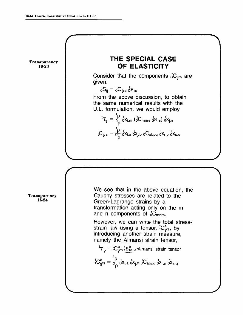
THE SPECIAL CASEOF ELASTICITY
Consider that the components JCi1S aregiven:
ts tc ta i} = a ijrs aE rsFrom the above discussion, to obtainthe same numerical results with theU.L. formulation, we would employ
tt _ P t (tc t) tTi} - op aXi,m a mnrs aE rs aXj.n
t
C Pt t C t tt ilS = 0 aXi,a aXj,b a abpq aXr,p aXs,q
P
We see that in the above equation, theCauchy stresses are related to theGreen-Lagrange strains by atransformation acting only on the mand n components of JCmnrs .
However, we can write the total stressstrain law using a tensor, ~C~rs, byintroducing another strain measure,namely the Almansi strain tensor,
tTi} = ~C~s !E~~/AlmanSi strain tensor
ttca _ P t t tc . t ttits - ~ aXi,a aXj.b a abpq aXr,p aXs,q
P

Definitions of the Almansi strain tensor:
~Ea = ! (I - ~XT ~X) / a:uk- 2 - - - aXJ-
ta 1(t t t t)tE·· = - tU" + tU' . - tUk' tUk .I'" 2 I.... ~.I .I.~
• A symmetric strain tensor, ~E~ = ~E;
• The components of ~E a are notinvariant under a rigid body rotationof the material.
• Hence, ~Ea is not a very useful strainmeasure, but we wanted to introduceit here briefly.
Topic Sixteen 16-15
Transparency16-25
Transparency16-26

16-16 Elastic Constitutive Relations in u'L.F.
Transparency16-27
Example: Uniaxial strain
t t~ 1 (t~)2of 11 = 0L +"2 0L
strain
1.0
-1.0=--_~~
Green-Lagrange
Engineering
~:.--_- Almansita
1.0 °L
Transparency16-28
It turns out that the use of ~Clrs withthe Almansi strain tensor is effectivewhen the U.L. formulation is used witha linear isotropic material law for largedisplacement / large rotation butsmall strain analysis.

'Ibpic Sixteen 16-17
• In this case, ~C~s may be taken as
t . atCijrS = A8ij- 8rs + f.L(8ir 8js + 8is 8jr)
• j
= tCiys constants
Practically the same response iscalculated using the T.L. formulationwith
JCijrS = A 8it 8rs + f.L(8ir 8js + 8is 8jr)\
Transparency16-29
= oC iys constants
MALLET ET AL
TL au L SOLUTIONS
r-~---{
Ii
TWELVE &-NODE ELEMENTSFOR HALF OF ARCH
Slide16·1
E =10 X 108 Ib./in.2
v= 0.2
04030.201
20
30
40
LOAD P [Ib]
VERTICAL DISPLACEMENT AT APEX Wo [in]
Load-deflection curve for a shallowarch under concentrated load
16-18 Elastic Constitutive Relations in V.L.F.
Transparency16-30
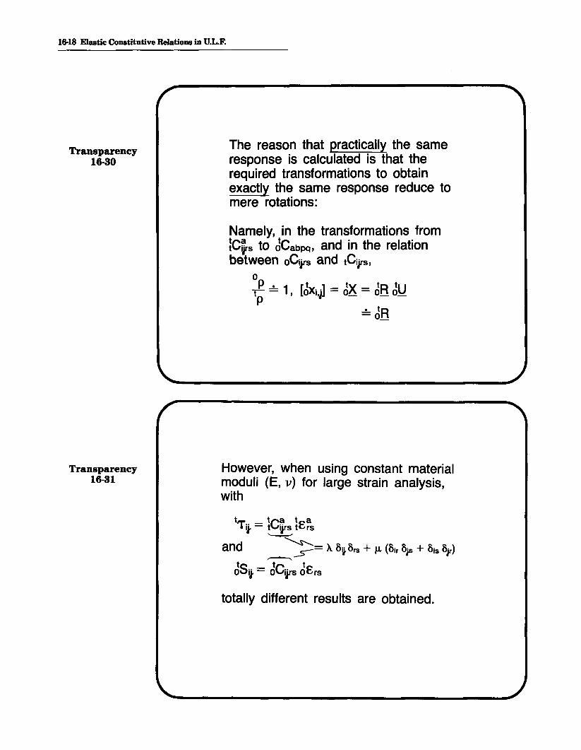
The reason that practically the sameresponse is calculated is that therequired transformations to obtainexactly the same response reduce tomere rotations:
Namely, in the transformations from~C~s to JCabPq, and in the relationbetween oCijrs and tCiys ,
o-.e ..!- 1 [JXi.~ = JX = JR Jutp -, r
..!- tR-0_
Transparency16-31
However, when using constant materialmoduli (E, v) for large strain analysis,with
totally different results are obtained.

Topic Sixteen 16-19
E= -:-:--_E--'-:-(1---,---:-.--:v)__=__:_(1 + v) (1 - 2v)
Transparency16-32
A
°Lt - tBefore, we used 0811 = E oE11.
. t - t aNow, we consider 'T11 = E tE 11 •
Consider the 1-D problem alreadysolved earlier:
Material constants E, v
Here, we haveTransparency
16-33
t tp1'11 = ~
A
U · tL 0L tAt E- t asing = + '-1, 'T11 = tE11,
obtain the force-displacementrelationship.
we

16·20 Elastic Constitutive Relations in u'L.F.
Transparency16-34
~tp = E2A (1 - C~r)-t-----jL-----+-- t~
Transparency16-35
Example: Corner under tip load
L
h A
L = 10.0 m}!! = _1h = 0.2 m L 50b = 1.0 mE = 207000 MPav = 0.3

Finite element mesh: 51 two-dimensionala-node elements
25 elements-I
Topic Sixteen 16-21
Transparency16-36
JRf'+t""-----"""1JI-'""'1J
not drawnto scale
25elements
:~I I I I I
All elements areplane strainelements.
Transparency16-37
Consider a nonlinear elastic analysis.For what loads will the T.L. and U.L.formulations give similar results?

16-22 Elastic Constitutive Relations in U.L.F.
Transparency16-38 For large displacement/large
rotation, but small strain conditions, the T.L. and U.L. formulations will give similar results.
- For large displacement/largerotation and large strain conditions, the T.L. and U.L. formulations will give different results,because different constitutiverelations are assumed.
Beam elements,.-:T.L. formulation
ol&-===----+-----+---_+_-o 5 10 15Vertical displacement of tip (m)
Results: Force-deflection curve• Over the range of loads shown, the T.L.
and U.L. formulations give practicallyidentical results
• The force-deflection curve obtained withtwo 4-node isoparametric beamelements is also shown.
62-D elements,T.L. and U.L.formulations~4
Force(MN)2
Transparency16-39

Deformed configuration for a load of 5 MN(2-D elements are used):
Undeformed 1Rr--------IIIIII Deformed, load = 1 MN
Deformed, load=5 MN
Numerically, for a load of 5 MN, we have,using the 2-D elements,
T.L. formulation U.L. formulationvertical tip
15.289 m 15.282 mdisplacement
The displacements and rotations are large.However, the strains are small - they canbe estimated using strength of materialsformulas:
Cbase = M~~2) where M • (5 MN)(7.5 m)
• 3%
Topic Sixteen 16-23
Transparency16-40
Transparency16-41

Contents:
Textbook:
Example:
References:
Topic 17
Modeling ofElasta-Plastic andCreepResponse Part I
• Basic considerations in modeling inelastic response
• A schematic review of laboratory test results, effects ofstress level, temperature, strain rate
• One-dimensional stress-strain laws for elasto-plasticity,creep, and viscoplasticity
• Isotropic and kinematic hardening in plasticity
• General equations of multiaxial plasticity based on ayield condition, flow rule, and hardening rule
• Example of von Mises yield condition and isotropichardening, evaluation of stress-strain law for generalanalysis
• Use of plastic work, effective stress, effective plasticstrain
• Integration of stresses with subincrementation
• Example analysis: Plane strain punch problem
• Example analysis: Elasto-plastic response up to ultimateload of a plate with a hole
• Computer-plotted animation: Plate with a hole
Section 6.4.2
6.20
The plasticity computations are discussed in
Bathe, K. J., M. D. Snyder, A. P. Cimento, and W. D. Rolph III, "On SomeCurrent Procedures and Difficulties in Finite Element Analysis of Elastic-Plastic Response," Computers & Structures, 12, 607-624, 1980.

17-2 Elasto-Plastic and Creep Response - Part I
References:(continued)
Snyder, M. D., and K. J. Bathe, "A Solution Procedure for Thermo-Elastic-Plastic and Creep Problems," Nuclear Engineering and Design, 64,49-80, 1981.
The plane strain punch problem is also considered in
Sussman, T., and K. J. Bathe, "Finite Elements Based on Mixed Interpolation for Incompressible Elastic and Inelastic Analysis," Computers& Structures, to appear.

. WE "D/SC.L{ SS"E D IN
THE "PRE\llO\A<; LEe
TU'?ES THE MODELING
OF ELASTIC. MA1E'RIALS
- l'NEA'R S~E-S<;
STRAIN LA~
Topic Seventeen 17-3
. WE Now WANT TO
.:DIS CIA':,'> TI1 E:
MO"DE LINlQ 0 F
IN ELASTIC HATER,ALS
- ELASTO-1>LASTICIT'f
ANb CREEP
- NONLINEAR S>T'RESc:,
STRAIN LAw
THE T. L. ANt> lA.L.
FO~t-IULAT10NS.
WE T'ROc.EEtl AS
FCLLoWS :
- WE DISC\i\S, 50 TS'RIEH'i
INELASTIC HATc"RIAL
~EI-\A'J\o'RSJ AS 0\3,-
SE'R'lJE'b IN LAB,-
O'Rt\T01<.'( TES-TS,
- WE J:> \ SC \A SS ~'R\E Fl'l
MObELlNE; OF SUCH
~ES'?ONse IN 1-1> ANAl'lSIS
- WE GENE~AU2E OuR
HObEUN6 CONSlbERA.lloNS
10 2-1) ANb3.-1)
STRES,S 5\1v..A.TI\lNS
Markerboard17-1

17-4 Elasto-Plastic and Creep Response - Part I
Transparency17-1
Transparency17-2
MODELING OF INELASTICRESPONSE:
ELASTO-PLASTICITY, CREEPAND VISCOPLASTICITY
• The total stress is not uniquelyrelated to the current total strain.Hence, to calculate the responsehistory, stress increments must beevaluated for each time (load) stepand added to the previous totalstress.
• The differential stress increment isobtained as - assuming infinitesimallysmall displacement conditions-
dO'ij- = C~s (ders - de~~)
where
C~s = components of the elasticitytensor
ders = total differential strain increment
de~~ = inelastic differential strainincrement

The inelastic response may occurrapidly or slowly in time, depending onthe problem of nature considered.Modeling:• In ~Iasticity, the model assumes that
de~s occurs instantaneously with theload application.
• In creep, the model assumes thatde~~ occurs as a function of time.
• The actual response in nature can bemodeled using plasticity and creeptogether, or alternatively using aviscoplastic material model.
- In the following discussion weassume small strain conditions,hence
• we have either a materiallynonlinear-only analysis
• or a large displacement/largerotation but small strainanalysis
Topic Seventeen 17-5
Transparency17-3
Transparency17-4

17-6 Elasto-Plastic and Creep Response - Part I
Transparency17-5
Transparency17-6
• As pointed out earlier, for the largedisplacement solution we would usethe total Lagrangian formulation andin the evaluation of the stress-strainlaws simply use
- Green-Lagrange strain componentfor the engineering strain components
and
- 2nd Piola-Kirchhoff stress components for the engineering stresscomponents
Consider a brief summary of someobservations regarding materialresponse measured in the laboratory
• We only consider schematically whatapproximate response is observed; no detailsare given.
• Note that, regarding the notation, no time, t,superscript is used on the stress and strainvariables describing the material behavior.

MATERIAL BEHAVIOR,"INSTANTANEOUS"
RESPONSE
Topic Seventeen 17-7
Transparency17-7
Tensile Test:
Crosssec:tionalarea Ao-z...
Assume• small strain conditions
• behavior in compressionis the same as in tension
Hence
e - eoe = --::---=-eop
(J' = -Ao
engineeringstress, (J
assumed
II
II
II
II
~ ", ', ,.",;'
......._-----
fracture
x ultimatestrain
5'
ngineeringtest strain, e
Constant temperature
Transparency17-8

17-8 Elasto-Plastic and Creep Response - Part I
Transparency17-9
Transparency17-10
Effect of strain rate:(J'
de. .dt Increasing
e
Effect of temperature(J'
temperature is increasing
e
Topic Seventeen 17-9
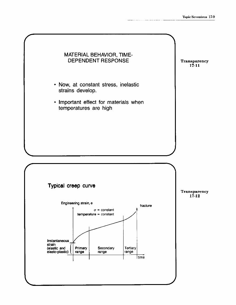
MATERIAL BEHAVIOR, TIMEDEPENDENT RESPONSE Transparency
17-11
• Now, at constant stress, inelasticstrains develop.
• Important effect for materials whentemperatures are high
Typical creep curveTransparency
17-12
Engineering strain, efracture
Tertiaryrange
Secondaryrange
a = constanttemperature = constant
Instantaneousstrain {(elastic and Primaryelasto-plastic) range
--:..+----=--+------'--~--+------l-
time

17-10 Elasto-Plastic and Creep Response - Part I
Transparency17-13
Effect of stress level on creep strain
ex
temperature = constant
x ---.s---::fracture
I
time
Effect of temperature on creep strainTransparency
17-14
e-S" fracture
x ""x
u=constant
time

MODELING OF RESPONSE
Consider a one-dimensional situation:tp
~tu h= A
~ jt.---tp'e ~ ~
L L
• We assume that the load is increasedmonotonically to its final value, P*.
• We assume that the time is "long" sothat inertia effects are negligible(static analysis).
Topic Seventeen 17-11
Transparency17-15
Load plasticityeffects
P*:..-....r_--,pt-redominate
.creep effects
fTransparency
17-16
time-dependent inelastic strainsare accumulated - modeled ascreep strains
'-"time inte~al t* (small)without time-dependentinelastic strains
time

17-12 Elasto-Plastic and Creep Response - Part I
strain
tOe
trr = E teE
telN = teP
·1·
rry- - - - -
Plasticity, uniaxial, bilinearmaterial model stressTransparency
17-17
Transparency17-18
Creep, power law material model:eC = ao <T
a, ta2
dtrr = E teE
telN = teC + teP
t* t time(small)
• The elastic strain is the same as inthe plastic analysis (this follows fromequilibrium).
• The inelastic strain is time-dependentand time is now an actual variable.

'Ibpic Seventeen 17-13
Viscoplasticity:
• Time-dependent response is modeledusing a fluidity parameter 'Y:
e = <1 + 'Y (~ - 1)E cry. . /
eVP
Transparency17-19
where
( _ ) _ { 0 I cr -< crycr cry -cr - cry I cr > cry
Transparency17·20
elasticstrain
elasticstrain
totalstrain. .
Increasing 'Y
Typical solutions (1-0 specimen):
steady~state depends onsolution increase in
total \ .strain fry as functionof eVP
time
non-hardening material
time
hardening material

17-14 Elasto-Plastic and Creep Response - Part I
Transparency17-21 PLASTICITY
Transparency17-22
• So far we considered only loadingconditions.
• Before we discuss more generalmultiaxial plasticity relations, considerunloading and cyclic loadingassuming uniaxial stress conditions.
• Consider that the load increases intension, causes plastic deformation,reverses elastically, and again causesplastic deformation in compression.
load
elastic
plastic
time

Bilinear material assumption, isotropichardening (T ET
(Ty
e
plastic strain (T~
e~
plastic strainI---+-l e~
Bilinear material assumption, kinematichardening (J ET
(Ty
plastic strain e~
e
Topic Seventeen 17-15
Transparency17-23
Transparency17-24

17-16 Elasto-Plastic and Creep Response - Part I
Transparency17-25
Transparency17-26
MULTIAXIAL PLASTICITY
To describe the plastic behavior inmultiaxial stress conditions, we use
• A yield condition
• A flow rule
• A hardening rule
In the following, we consider isothermal(constant temperature) conditions.
These conditions are expressed using astress function tF.
Two widely used stress functions are the
von Mises function
Drucker-Prager function

Topic Seventeen 17-17
von Mises
tF =~ ts ts.. _ tK2 I} II'
Transparency17-27
Drucker-Prager
t ~a._II ; t(j =3
1 t t- s .. s ..2 If If
We use both matrix notation and indexnotation: Transparency
17-28
dCT11dCT22dCT33dCT12dCT23dCT31
dCT =
matrix notationnote that both de~2
and de~1 are added
de~1de~2
de~3
de~2 + de~1
de~3 + de~2
de~3 + de~1

17-18 Elasto-Plastic and Creep Response - Part I
Transparency[ de~, de~2 de~3 ]17-29
d P- de~1 de~2 de~3eij -de~1 de~2 de~3
indexnotation
[ dcrl1 d<J12 dcr'3 ]d<J~ = d<J21 d<J22 d<J23
d<J31 d<J32 d<J33
Transparency17-30
The basic equations are then (von Mises tF):1) Yield condition
tF C<Jij, tK) = 0
current str~sses~ function ofplastic strains
tF is zero throughout the plastic response
• 1-D equivalent: ~ C<J2 - t<J~) = 0(uniaxial stress) 7 ~
current stresses function ofplastic strains.

2) Flow rule (associated rule):
P t atFdeii. = X. -at
I ITi}
where tx. is a positive scalar.
• 1-D equivalent:
d P 2 t\ te11 = 3 I\. IT
d P 1 t\ te22 = - 3 I\. IT
d P 1 t\ te33 = - 3 I\. IT
3) Stress-strain relationship:
dIT = CE (d~ - d~P)
• 1-D equivalent:
dIT = E (de11 - de~1)
Thpic Seventeen 17-19
Transparency17-31
Transparency17-32

17-20 Elasto-Plastic and Creep Response - Part I
Transparency17-33
Transparency17-34
Our goal is to determine CEP such that
dO" = CEP de- ~-
\instantaneous elastic-plastic stress-strain matrix
General derivation of CEP:
Define

Using matrix notation,
Topic Seventeen 17-21
Transparency17-35
tgT = [tq11 : tq : tq :: 22: 33:
't. t I
i P22: P33 itIt It]P12 i P23 i P31
We now determine tx. in terms of de:
Using tF = 0 during plastic deformations,
t atF atF pd F = -t- d(Jii. + --:::t=Pat deii.a(Ji} I ei} I
= 'gT do- - 'ET~tx.tg
=0
Transparency17-36

17-22 Elasto-Plastic and Creep RespoDse - Part I
Transparency17-37
Transparency17-38
Also
tgTdO" = tgT (QE (d~ - d!t))L . t
The flow rule assumption may bewritten as
HencetgT dO" = tgT (CE (d~ _ tA tg))= tA tQT tg-
Solving the boxed equation for tA gives
Hence we can determine the plasticstrain increment from the total strainincrement: I ..
tota strain Increment
p tgTCEd~~tde = ( ) 9~ - tQTtg + tgT CEtg
plastic strainincrement

Example: Von Mises yield condition,isotropic hardening
Two equivalent equations:
Topic Seventeen 17-23
Transparency17-39
Transparency17-40
t ~O"Y=T
(trr • t )2 (t t)2 (t t)2
~~\+t-t~/?~principal stresses
tF _ 1 t t t. t _ 1 t 2- 2: sij.~ K , K - 3 0"Y
~5 t
d · . t " (Tmm ~eVlatonc s resses: Sij- = (Tij- - -3- Uij

17-24 Elasto-Plastic and Creep Response - Part I
Transparency17-41 Yield surface
for plane stressEnd view ofyield surface
Transparency17-42
We now compute the derivatives of theyield function.
First consider tpy.:
t _ atF _ a (1 t t 1 t 2py. - - atef! - - atef! 2 sy. SiJ- - 3 O'y)
II' t(J"it fixed II'
(t(J"ij- fixed implies tSij- is fixed)

What is the relationship between tcryand the plastic strains?
We answer this question using theconcept of "plastic work".
• The plastic work (per unit volume) isthe amount of energy that isunrecoverable when the material isunloaded.
• This energy has been used increating the plastic deformationswithin the material.
• Pictorially: 1·0 example
'Ibpic Seventeen 17-25
Transparency17-43
stress
~et
Shaded area equalsplastic work t wp:
'----------strain
Transparency17-44
rtePIjo
• In general, 'Wp =Jo Tay.de~

17-26 Elasto-Plastic and Creep Response - Part I
Transparency17-45
Transparency17-46
Consider 1-0 test results: the currentyield stress may be written in terms ofthe plastic work.
Shaded area =:
Wp = ~ (~T - i) (t(1~ - (1~)
'---------- strain
We can now evaluate tPij- - whichcorresponds to a generalization of the1-D test results to multiaxial conditions.
t _ 2 t (d\JY atWp)/at
(1YPij- - 3 (]'Y dtWp ater ate~
\ t /.

(effective stress)
(increment iiieffective
t plastic strain)result is obtained
Alternatively, we could have used thatdtWp = tcr dtet
where
and then the sameusing
t .. _ 2 t (d\ry ateP
)Pit - 3 (J'y dteP ate~
Next consider tq~:
'Ibpic Seventeen 17-27
Transparency17-47
Transparency17-48

17-28 Elasto·Plastic and Creep Response - Part 1
We can now evaluate gEP:
symmetric
Transparency17-49
cEP = _E_- 1+v
de11 de22 2 de12
2'
I I I1 - V (') V 'I I I Q. 1 , I-- - ~ 511 I -- - ~ 511 522 •.• - P 511 512 •.•1-2v 11-2v I I I- - - - - - - - - - - - - - - - -:2: -1- I" - - - - - - I .......
I 1 - V (') I I Q. ' , II 1 _ 2v - ~ 522 I··· I - P 522 512 I···L 1_ I" - - - - - - I -
I .•• I - ~ '533 1512 I ...I I I
-'1-----2 '
I - -~('512) I •.•I 2 I-------1-
I •••I
Transparency17-50
3 1 ( 1 )where 13 = - f22 O"y 1 + g E ET 1 + v
3 E - ET E
Evaluation of the stresses at time t+ ~t:
The stress integrationmust be performed ateach Gauss integrationpoint.

We can approximate the evaluation ofthis integral using the Euler forwardmethod.
• Without subincrementation:
J:t+~le I+~I I- e e
Ie CEPd~ . CEP
,d~"/ - - -- t
• With n subincrements:
den ~t
t+~--s-n
+ ...
Topic Seventeen 17-29
Transparency17-51
Transparency17-52
den
t+(n-1)Lh

17-30 Elasto-Plastic and Creep Response - Part I
Transparency17-53
Pictorially:
tsubincrements
t+8t
Transparency17-54
Summary of the procedure used tocalculate the total stresses at timet+dt.Given:
STRAIN = Total strains at time t+dtSIG = Total stresses at time tEPS = Total strains at time t
(a) Calculate the strain incrementDELEPS:
DELEPS = STRAIN - EPS

(b) Calculate the stress incrementDELSIG, assuming elastic behavior:
DELSIG = CE * DELEPS
(c) Calculate TAU, assuming elasticbehavior:
TAU = SIG + DELSIG
(d) With TAU as the state of stress,calculate the value of the yieldfunction F.
(e) If F(TAU) < 0, the strain incrementis elastic. In this case, TAU iscorrect; we return.
(f) If the previous state of stress wasplastic, set RATIO to zero and goto (g). Otherwise, there is atransition from elastic to plastic andRATIO (the portion of incrementalstrain taken elastically) has to bedetermined. RATIO is determinedfrom
F (SIG + RATIO * DELSIG) = 0
since F = 0 signals the initiation ofyielding.
Topic Seventeen 17-31
Transparency17-55
Transparency17-56

17-32 Elasto·Plastic and Creep Response - Part I
Transparency17-57 (9) Redefine TAU as the stress at start
of yieldTAU = SIG + RATIO * DELSIG
and calculate the elastic-plasticstrain increment
DEPS = (1 - RATIO) * DELEPS
(h) Divide DEPS into subincrementsDDEPS and calculate
TAU ~ TAU + CEP * DDEPSfor all elastic-plastic strainsubincrements.

Topic Seventeen 17-33
1........--- 2b ---I.~I
p
Slide17-1
PLASTIC ZONE
Plane strain punch problem
Slide17-2
P/l Ii.I
z 10- .....I
lOl- A ,,"~.
Finite element model of punch problem

17-34 Elasto-Plastic and Creep Response - Part I
Slide17-3
STRESS, 0' lplll
'00
"200 Ib.'CW.. h••
\. "... "".. T,.- - - THEOR£TICAL
-- - -----0I 0 2.0 30DISTANCE FROM CENTERLINE, b (inl
Solution of Boussinesq problem-2 pt. integration
Slide17-4
STRESS, 0' lpoi)
200
'00
• VIZ
• er".. T,Z
- - - TH(ORETlCAl
-----------10 2.0 30DISTANCE FROM CENTERLINE, b (in)
Solution of Boussinesq, problem-3 pt. Integration

APPLIEDLOAD,P/2kb
p
~• 2 pi In,a S"pI inl
Topic Seventeen 17-35
Slide17-5
0.05 QIQ 0.'5DISPLACEMENT, ,,/b
0.20
Load-displacement curves for punch problem

17-36 Elasto-Plastic and Creep Response - Part I
Transparency17-58
Transparency17-59
Limit load calculations:
p
rTTTTl
o
• Plate is elasto-plastic.
Elasto-plastic analysis:
Material properties (steel)a
740 -I--
a(MPa)
~Er = 2070 MPa, isotropic hardening
'-E=207000 MPa, v=0.3
e• This is an idealization, probably
inaccurate for large strain conditions(e > 2%).

TIME = 0LOAD = 0.0 MPA
TIME - 41LOAD - 512.5 MPA
TIME - 62LOAD - 660.0 MPA
=====..:=r~--.,.,......~"-----....----....~-----,.._-...-.~....,....,••••1••••1...,!!!!....~....
\
Topic Seventeen 17-37
ComputerAnimationPlate with hole

Contents:
Textbook:
References:
Topic 18
Modeling ofElasto-Plastic andCreepResponse Part II
• Strain formulas to model creep strains
• Assumption of creep strain hardening for varying stresssituations
• Creep in multiaxial stress conditions, use of effectivestress and effective creep strain
• Explicit and implicit integration of stress
• Selection of size of time step in stress integration
• Thermo-plasticity and creep, temperature-dependency ofmaterial constants
• Example analysis: Numerical uniaxial creep results
• Example analysis: Collapse analysis of a column withoffset load
• Example analysis: Analysis of cylinder subjected to heattreatment
Section 6.4.2
The computations in thermo-elasto-plastic-creep analysis are describedin
Snyder, M. D., and K. J. Bathe, "A Solution Procedure for Thermo-Elastic-Plastic and Creep Problems," Nuclear Engineering and Design, 64,49-80, 1981.
Cesar, F., and K. J. Bathe, "A Finite Element Analysis of QuenchingProcesses," in Numerical Methods jor Non-Linear Problems, (Taylor,C., et al. eds.), Pineridge Press, 1984.

18-2 Elasto-Plastic and Creep Response - Part II
References:(continued)
The effective-stress-function algorithm is presented in
Bathe, K. J., M. Kojic, and R. Slavkovic, "On Large Strain Elasto-Plasticand Creep Analysis," in Finite Element Methods for Nonlinear Problems (Bergan, P. G., K. J. Bathe, and W. Wunderlich, eds.), SpringerVerlag, 1986.
The cylinder subjected to heat treatment is considered in
Rammerstorfer, F. G., D. F. Fischer, W. Mitter, K. J. Bathe, and M. D.Snyder, "On Thermo-Elastic-Plastic Analysis of Heat-Treatment Processes Including Creep and Phase Changes," Computers & Structures,13, 771-779, 1981.

CREEPWe considered already uniaxialconstant stress conditions. A typicalcreep law used is the power creep laweO = ao (181 t~.
time
Aside: other possible choices for the creeplaw are
• eC= ao exp(a1 cr) [1 - exp(-a2 c~:r4 t)]
+ as t exp(ae cr)
• eC
= (ao (cr)a1) (ta2 + a3 t84 + as ta6) exp (te +-2~3.16)~'-'
temperature. in degrees C
We will not discuss these choices further.
Topic Eighteen 18·3
Transparency18-1
Transparency18-2

18-4 Elasto-Plastic and Creep Response - Part II
Transparency18-3
The creep strain formula eC = aO (Tal ta2
cannot be directly applied to varying stresssituations because the stress history doesnot enter directly into the formula.
-----(12Ccreep strain not affected
_-.J~---(11 by stresshistory priorto t1
time
"time
decrease in the creepstrain is unrealistic
f----.......-------(11
~---,...--------(12
Example:
J I:eC
Transparency18-4

The assumption of strain hardening:
• The material creep behavior dependsonly on the current stress level andthe accumulated total creep strain.
• To establish the ensuing creep strain,we solve for the "effective time" usingthe creep law:
_ totally unrelatedteC = aQ \:ra1~~ to the physical
time
(solve for t)
The effective time is now used in thecreep strain rate formula:
Now the creep strain rate dependson the current stress level and onthe accumulated total creep strain.
Topic Eighteen 18-5
Transparency18-5
Transparency18-6

18-6 Elasto-Plastic and Creep Response - Part II
Transparency18-7
Transparency18-8
Pictorially:• Decrease in stress
to'-1-__------------
4---1------------- a'
+-------------- time0'2
material/response
~__~;::::::::.. a'
~~------------time
• Increase in stress
to'-+--------------~------........'-------- a'
+---------------- time0'2
material--.-:::::::.~---=--..:::>
response
-4£:..-------------- time

• Reverse in stress (cyclic conditions)
-+----+--------time
<12L-- _
_ _ ~<12 curve- - _ - - --s-- <11 curve
/ --,/ -/ "",/
-fI""--------"-.:-------- time
MULTIAXIAL CREEP
The response is now obtained using(t+tl.te
t+dt(T = t(T +A~ - CE d (~ - ~c)
As in plasticity, the creep strains inmultiaxial conditions are obtained by ageneralization of the 1-0 test results.
Topic Eighteen 18-7
Transparency18-9
Transparency18-10

18-8 Elasto-Plastic and Creep Response - Part II
Transparency18-11 We define
,....---.....t- 3 t t(J = 2 Si~ sy. (effective stress)
t-Ce = (effective strain)
Transparency18-12
and use these in the uniaxial creeplaw:
eC = ao cr81{82
The assumption that the creep strainrates are proportional to the currentdeviatoric stresses gives
te' C t ts (' M' I t" 'ty)i~ = ry i~ as In von Ises p as ICI
try is evaluated in terms of the effectivestress and effective creep strain rate:
3 t.:.Ct ery = 2 tcr

Using matrix notation,
d~c = Coy) (D to") dt" ;/
deviatoricstresses
For 3-D analysis,
Topic Eighteen 18-9
Transparency18-13
D=
! -~ -~
! -~
!
symmetric1
11
• In creep problems, the timeintegration is difficult due to the highexponent on the stress.
• Solution instability arises if the Eulerforward integration is used and thetime step ~t is too large.- Rule of thumb:
A -c -< _1 (t-E)L.l~ - 10 ~
• Alternatively, we can use implicitintegration, using the a-method:
HaatO" = (1 - a) to" + a HatO"
Transparency18-14

18·10 Elasto-Plastic and Creep Response - Part II
Transparency18-15
Iteration algorithm:t+~ta(l-1) = ta +_(k) _
cE [~(1-1 L ~t t+a~t'Y~k-=-1{) (0 t+a~t!!~k-=-1{»)]
we iterate ateach integrationpoint
r
xxx
x
x
k = iteration counter at each integration point
s
Transparency18-16 • a>V2 gives a stable integration
algorithm. We use largely a = 1.0.
• In practice, a form of NewtonRaphson iteration to accelerateconvergence of the iteration canbe used.

• Choice of time step dt is nowgoverned by need to convergein the iteration and accuracyconsiderations.
• Subincrementation can be employed.
• Relatively large time steps can beused with the effective-stressfunction algorithm.
THERMO-PLASTICITY-CREEPstress
O'y3-+-__Plasticity: O'y2-+-_-+-
0'y 1---l---74L...-----r--Increasingtemperature
strain
Topic Eighteen 18-11
Transparency18-17
Transparency18-18
Creep:
creepstrain
Increasingtern erature
time

18-12 Elasto-Plastic and Creep Response - Part II
Transparency18-19
Transparency18-20
Now we evaluate the stresses usingt+~te
I+AIQ: = IQ: + r, -TCEd(~ _ ~p _ ~c _ ~TH)J,~ .-5~
thermalstrains
Using the ex-method,
I+AIQ: = t+AICE{ [~ _ ~p _ ~c _ ~TH]
+[I~ _ I~P _ t~C _ I~TH]}
where
e = I+Ale - Ie- --
and~p = Llt (t+a~t~) (D t+a~ta)
~c = Llt (t+a~t'Y) (D t+a~ta)
e;H = (t+~ta t+~t8 - ta t8) Oi.j-
where
ta = coefficient of thermal expansion attime t
t8 = temperature at time t
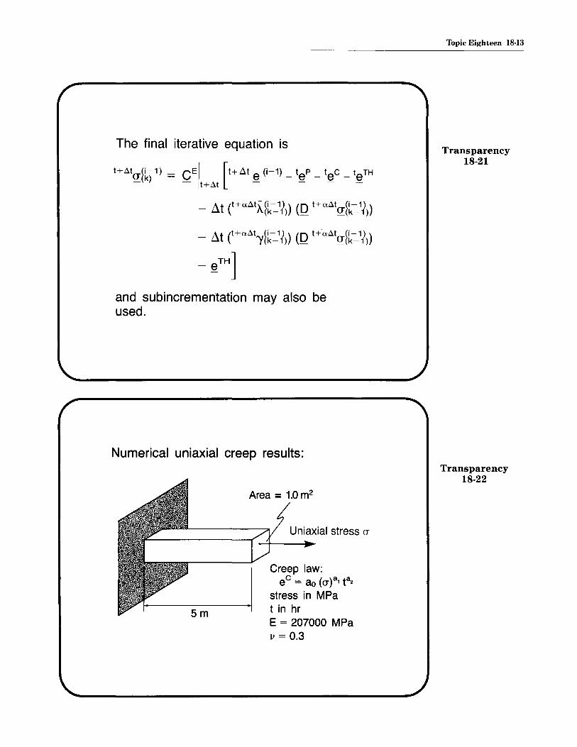
The final iterative equation is
- Lit C+Cldt~~k~1{») (0 t+Cldt(J~k~1{»)
- Lit (t+Cldt)'~k~1{») (0 t+Cldt(J~k~1{»)
_~TH]
and subincrementation may also beused.
Numerical uniaxial creep results:
Topic Eighteen 18-13
Transparency18-21
5m
Area =1.0 m2
Uniaxial stress 0"
Creep law:eC = ao (0")a1 ta2
stress in MPat in hrE = 207000 MPav = 0.3
Transparency18-22
18-14 Elasto-Plastic and Creep Response - Part II
Transparency18-23
The results are obtained using twosolution algorithms:
• ex = 0, (no subincrementation)• ex = 1, effective-stress-function
procedure
In all cases, the MNO formulation isemployed. Full Newton iterationswithout line searches are used with
ETOL=0.001RTOL=0.01RNORM = 1.0 MN
Transparency18-24
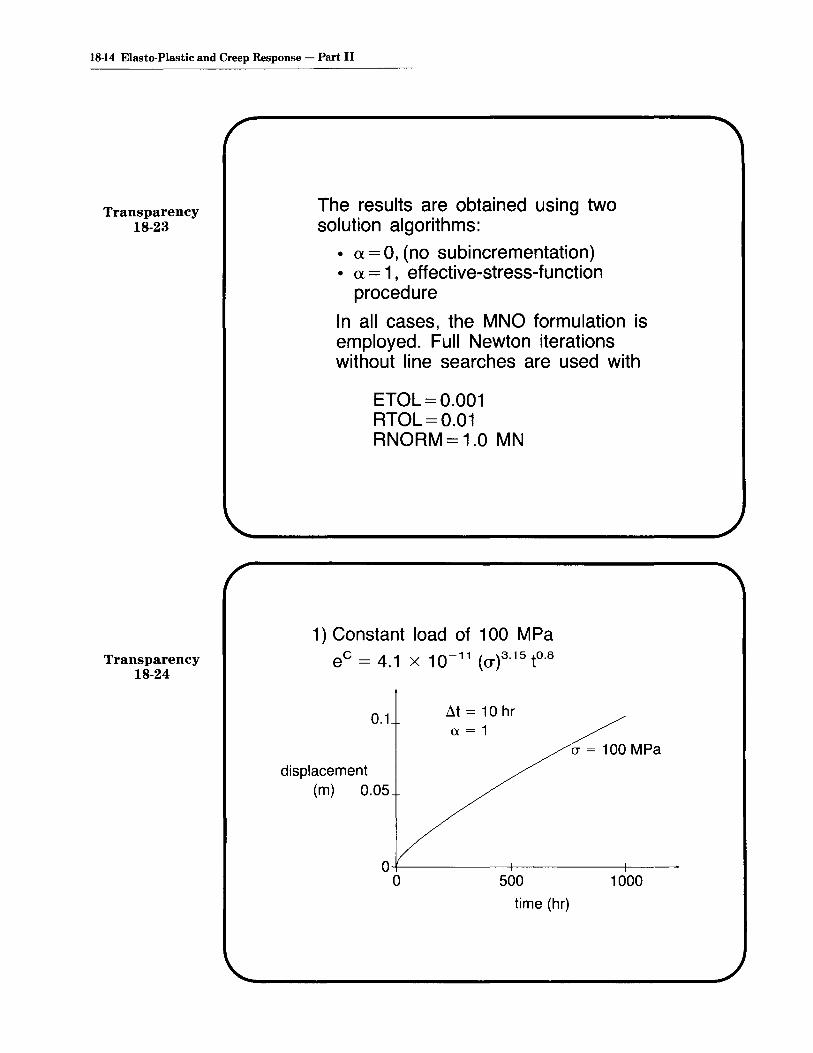
1) Constant load of 100 MPaeC = 4.1 x 10~11 (a)3.15 to.8
0.1 ~t = 10 hra=1
(J' = 100 MPa
displacement(m) 0.05
1000500
time (hr)
0+-------+------+----o
Topic Eighteen 18-15
Transparency18-25
at = 10 hr<x=1
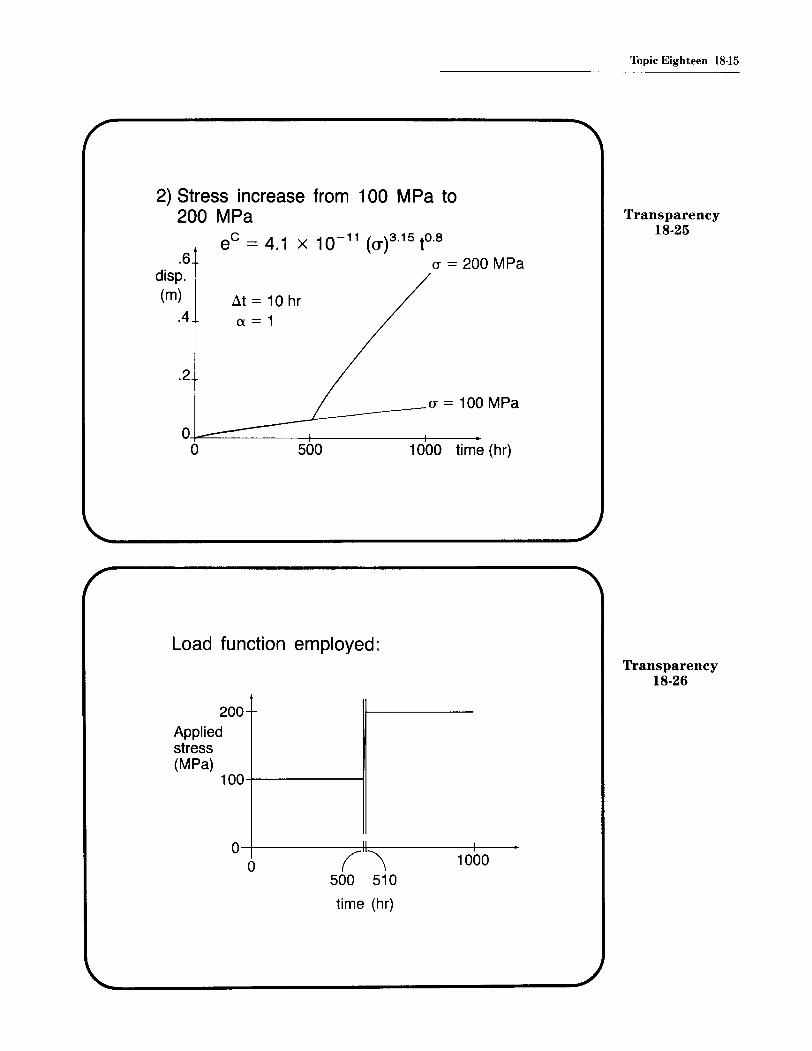
2) Stress increase from 100 MPa to200 MPa
eC = 4.1 x 10⁻¹¹ (cr)3.15 to.8
(J = 200 MPa.6disp.(m)
.4
.2
1000 time (hr)5000-+-==---- ----+ -+-__
o
(J = 100 MPaL---~
Load function employed:Transparency
18-26
200Appliedstress(MPa)
100+-------i1
1000O-+---------,H:-II -----+---
o (\500 510
time (hr)

18-16 Elasto-Plastic and Creep Response - Part II
~t = 10 hr(1=1
0.1disp.(m)0.0
3) Stress reversal from 100 MPa to-100 MPa
eC = 4.1 x 10⁻¹¹ (cr)3.15 to.8
(J' = 100 MPa
Transparency18-27
500 1000 time (hr)
-0.05
Transparency18-28
4) Constant load of 100 MPaeC = 4.1 x 10⁻¹¹ (cr)3.15 t°.4
.01
disp.(m)
.005
~t = 10 hr(1=1 (J' = 100 MPa
1000 time (hr)500
0+- --+ -+-__
a

Topic Eighteen 18-17
Transparency18-29
(T = 100 MPa
5) Stress increase from 100 MPa to200 MPa.06 eC = 4.1 x 10⁻¹¹ (cr)3.15 t°.4
8t=10hrex = 1
.04disp.(m)
.02
1000 time (hr)500
0,+-- --+ +- __
o
(T = 100 MPa
6) Stress reversal from 100 MPa to-100 MPa
eC = 4.1 x 10⁻¹¹ (cr)3.15 t°.4.01 8t = 10 hr
disp. ex = 1(m)
.005
Transparency18-30
O'+- -+~;;;:::__----+-------
1000 time (hr)
(T = -100 MPa-.005
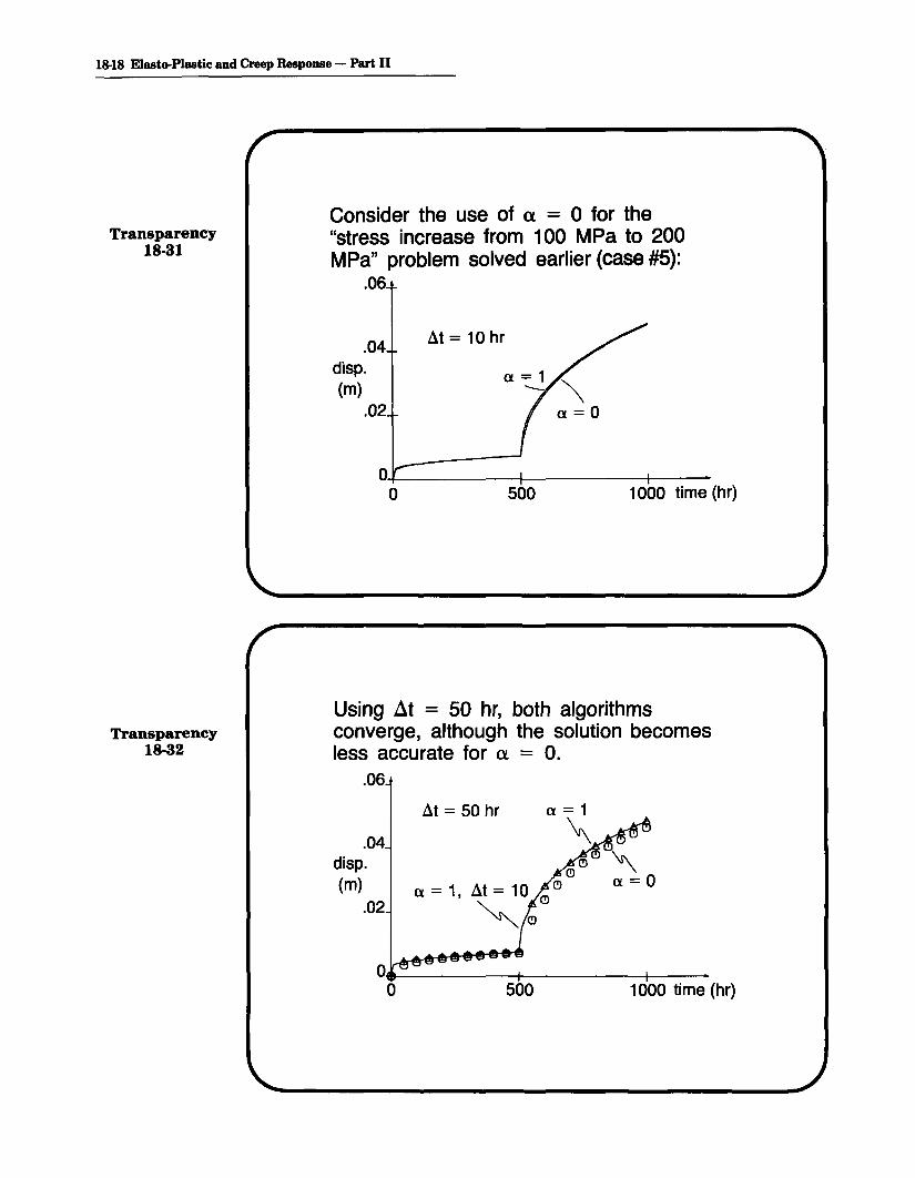
18-18 Elasto-Plastic and Creep Response - Part II
Transparency18-31
Consider the use of a = 0 for the"stress increase from 100 MPa to 200MPa" problem solved earlier (case #5):
.06
.04disp.(m)
.02
~t = 10 hr
1000 time (hr)500
0,+- -+ +-__o
Transparency18-32
Using dt = 50 hr, both algorithmsconverge, although the solution becomesless accurate for a - O.
.06
.04disp.(m)
.02
~t = 50 hr
(!)(!)
(!)
<X = 1 ~t = 10 (!), (!)
~ (!)
1000 time (hr)5000,_------+------4----o

Topic Eighteen 18-19
Using dt = 100 hr, (X = a does notconverge at t = 600 hr. (X = 1 still givesgood results.
.06
Transparency18-33
~t=100hr.04
disp.
(m) a = 1, ~t = 10 hr.02 ~
a=1--1000 time (hr)500
Oe--------t-~---__+_-o
E=2x10⁶ KPav=O.Oplane stressthickness = 1.0 m
Example: Column with offset load
R
-11-0.75
Transparency18-34
10 m
Euler buckling load = 41 00 KN

18-20 Elasto-Plastic and Creep Response - Part II
Transparency18-35
Transparency18-36
Goal: Determine the collapse responsefor different material assumptions:
Elastic
Elasto-plastic
Creep
The total Lagrangian formulation isemployed for all analyses.
Solution procedure:
• The full Newton method withoutline searches is employed with
ETOL=0.001
RTOL=0.01
RNORM = 1000 KN

Mesh used: Ten 8-node quadrilateralelements
~ 3 x 3 Gauss integration~ used for all elements
Elastic response: We assume that thematerial law is approximated by
ts tc to ij = 0 ijrs OCrs
where the components JCijrS areconstants determined by E and v (aspreviously described).
Topic Eighteen 18·21
Transparency18-37
Transparency18-38
5000
Appliedforce(KN) 2500
Eulerbuckling ioad
tPPlied forcenLateraljJr displacement
O+-----t----+----+---a 2 4 6
Lateral displacement of top (m)

18-22 Elasto-Plastic and Creep Response - Part II
Transparency18-39
Transparency18-40
Elasto-plastic response: Here we use
ET = 0cry = 3000 K Pa (von Mises yieldcriterion)
and
JI+At E
t+LltS = cis + o-CEP doE0_ - tE 0- -
0-
whereoCEP is the incremental elastoplastic constitutive matrix.
Plastic buckling is observed.
Elastic2000
Appliedforce(KN)
1000Elasto-plastic
O+---t-----t---+---+---+---o .1 .2 .3 .4 .5
Lateral displacement of top (m)

Creep response:
• Creep law: eC = 10-16(cr)3 t (t inhours)No plasticity effects are included.
• We apply a constant load of 2000K N and determine the time history ofthe column.
• For the purposes of this problem, thecolumn is considered to havecollapsed when a lateral displacementof 2 meters is reached. Thiscorresponds to a total strain of about2 percent at the base of the column.
We investigate the effect of differenttime integration procedures on theobtained solution:
• Vary At (At = .5, 1, 2, 5 hr.)
• Vary ex (ex=O, 0.5, 1)
'Ibpic Eighteen 18-23
Transparency18-41
Transparency18-42

18-24 Elasto-Plastic and Creep Response - Part II
Transparency18-43
Collapse times: The table below liststhe first time (in hours) for which thelateral displacement of the columnexceeds 2 meters.
a=O a=.5 a=1dt=.5 100.0 100.0 98.5dt= 1 101 101 98dt=2 102 102 96dt=5 105 105 90
Pictorially, using dt =0.5 hr., ex =0.5,we haveTransparency
18-44Time= 1 hr
(negligible creepeffects)
Time=50 hr(some creep
effects)
IfIIIfIII
Time= 100 hr(collapse)

Topic Eighteen 18-25
1.0
0.5
Transparency18-45
Choose at = 0.5 hr.- AI1 solution points are connected
with straight lines.2.5
a=1 a=Ocollapse '- ~ a = .5
2.0+----~--------IJ~--
Lateraldisp. 1.5(m)
20 40 60 80 100' 120time (hr)
Effect of a: Choose at=5 hr.- All solution points are connected
with straight lines.2.5
collapse2.0,-+--__----:. ---->~-~
Lateral 1.5disp.(m) 1.0
0.5
Transparency18-46
O+---+---+---+----f--t---......o 20 40 60 80 100 120
time (hr)

18-26 Elasto-Plastic and Creep Response - Part II
Transparency18-47
We conclude for this problem:
• As the time step is reduced, thecollapse times given by ex = 0,ex = .5, ex = 1 become closer. Forat = .5, the difference in collapsetimes is less than 2 hours.
• For a reasonable choice of timestep, solution instability is not aproblem.

r
I=-"T
II
zf-rl~2Ra
I I IS: : S!IL..............--JIL-IL.....L..I..L.IL..&II~I..LIu..111'"'r',~
Ra = 25 mm ~
Analysis of a cylinder subjected to heat treatment
Topic Eighteen 18-27
Slide18-1
1400 70
/\ k SlidecWs/kgDC W/mDC 18-2
/\c
800
400 20
o 200 400 600 ODC 900
Temperature-dependence of the specific heat,~, and the heat conduction coefficient, k.

18-28 Elasto·Plastic and Creep Response - Part II
Slide18-3
1.2
0.4
----------------, .40
v
.32
Temperature-dependence of the Young's modulus, E,Poisson's ratio, II, and hardening modulus, ET
600 ,..-----------------..
Slide18-4
200
o
Temperature-dependence of the material yield stress

Thpic Eighteen 18-29
Slide18-5
600 0 °c 900o
-2
-6
-4
a 1O-5oc-/r------- --.
2
Temperature-dependence of the instantaneous coeffiCientof thermal expansion (including volume change due to
phase transformation), a
,.,..-------------------,
1SII+---+------t---+---"~_+---\--I
_+---+------t---""''''<:::'""""-+--_+*-----'I
t·IU'5_
D.5
J.j
Slide18-6
--fI fI.l fl.• (J.f II r/Ra Lfl
The calculated transient temperature field

18-30 Elasto-Plastic and Creep Response - Part II
Slide18-7
1000 r-------------------------~
e °c r----------=-==~_600
10 3D to 60 txI 100 t.oc JOt)
temperatureIn element "
2 J. 6810
surfacet~mperaturl
1 J. 6 8 1
I§ranSformar-;;;: --------mr~rval
--------====~~=--
600
100
Surface and core temperature; comparison betweenmeasured and calculated results
Slide18-8
1000..----------------------,
500
Nmm2
-500Urr
-1000-'------------------~
Measured residual stress field

1000.,-------------------,
Topic Eighteen 18-31
Slide18-9
500
o
-500
\\
\
\ 1Ra0.8 " 1.0
\\
\\
\
-1000.L-------------------'
Calculated residual stress field

Contents:
Textbook:
References:
Topic 19
Beam, Plate, andShell ElementsPart I
• Brief review of major formulation approaches
• The degeneration of a three-dimensional continuum tobeam and shell behavior
• Basic kinematic and static assumptions used
• Formulation of isoparametric (degenerate) general shellelements of variable thickness for large displacementsand rotations
• Geometry and displacement interpolations
• The nodal director vectors
• Use of five or six nodal point degrees of freedom,theoretical considerations and practical use
• The stress-strain law in shell analysis, transformationsused at shell element integration points
• Shell transition elements, modeling of transition zonesbetween solids and shells, shell intersections
Sections 6.3.4, 6.3.5
The (degenerate) isoparametric shell and beam elements, including thetransition elements, are presented and evaluated in
Bathe, K. J., and S. Bolourchi, "A Geometric and Material NonlinearPlate and Shell Element," Computers & Structures, 11, 23-48, 1980.
Bathe, K. J., and L. W. Ho, "Some Results in the Analysis of Thin ShellStructures," in Nonlinear Finite Element Analysis in StructuralMechanics, (Wunderlich, W., et al., eds.), Springer-Verlag, 1981.
Bathe, K. J., E. Dvorkin, and L. W. Ho, "Our Discrete Kirchhoff and Isoparametric Shell Elements for Nonlinear Analysis-An Assessment,"Computers & Structures, 16, 89-98, 1983.
•

19-2 Beam, Plate and Shell Elements - Part I
References:(continued)
The triangular flat plate/shell element is presented and also studied in
Bathe, K. J., and L. W. Ho, "A Simple and Effective Element for Analysis of General Shell Structures," Computers & Structures, 13, 673681, 1981.

STRUCTURAL ELEMENTS
• Beams
• Plates
• Shells
We note that in geometrically nonlinearanalysis, a plate (initially "flat shell")develops shell action, and is analyzedas a shell.
Various solution approaches have been proposed:
• Use of general beam and shelltheories that include the desirednonlinearities.
- With the governing differentialequations known, variationalformulations can be derived anddiscretized using finite elementprocedures.
- Elegant approach, but difficultiesarise in finite element formulations:• Lack of generality• Large number of nodal degrees
of freedom
Topic Nineteen 19-3
Transparency19-1
Transparency19-2

19-4 Beam, Plate and Shell Elements - Part I
Transparency19-3
• Use of simple elements, but a largenumber of elements can modelcomplex beam and shell structures.
- An example is the use of 3-nodetriangular flat plate/membraneelements to model complex shells.
- Coupling between membrane andbending action is only introducedat the element nodes.
- Membrane action is not very wellmodeled.
bendingf membraneartificial
.ISs stiffness
I
\~3 / degree of freedom with\/_~ artificial stiffness~'/..z
L5}~--xl
X1
Stiffness matrix inlocal coordinatesystem (Xi).
Example:Transparency
19-4

• Isoparametric (degenerate) beam andshell elements.
- These are derived from the 3-Dcontinuum mechanics equationsthat we discussed earlier, but thebasic assumptions of beam andshell behavior are imposed.
- The resulting elements can beused to model quite general beamand shell structures.
We will discuss this approach in somedetail.
Basic approach:
• Use the total and updated Lagrangianformulations developed earlier.
Topic Nineteen 19-5
Transparency19-5
Transparency19-6

19-6 Beam, Plate and Shell Elements - Part I
Transparency19-7
Transparency19-8
We recall, for the T.L. formulation,
f HAtS.. ~HAtE .. 0dV _ HAt(jJ}Jov 0 II'U 0 II' - ;:IL
Linearization ~
£'v OCiirs oers 80ei~ °dV +f,v JSi~8o"ly. °dV
= HAtm - f,v JSi~8oey.°dV
Also, for the U.L. formulation,
JVHA~Sij.8HA~Eij. tdV = HAtm
Linearization ~
Jv tCifs ters 8tei} tdV +Jv~i~8t'T\ij. tdV
= H At9R - f",t'Tij. 8tei}tdV

• Impose on these equations the basicassumptions of beam and shell -action:
1) Material particles originally on astraight line normal to the midsurface of the beam (or shell)remain on that straight linethroughout the response history.
For beams, "plane sections initiallynormal to the mid-surface remainplane sections during the responsehistory".
The effect of transverse sheardeformations is included, andhence the lines initially normal tothe mid-surface do not remainnormal to the mid-surface duringthe deformations.
Topic Nineteen 19-7
Transparency19-9
Transparency19-10
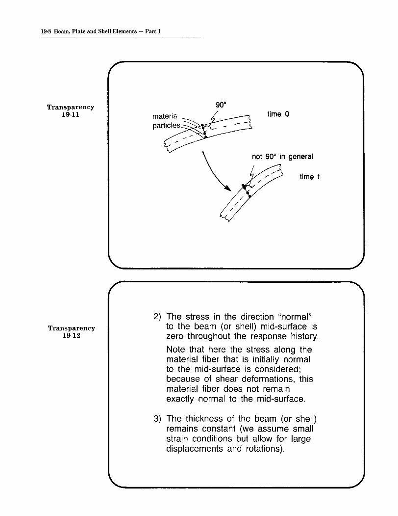
19-8 Beam, Plate and Shell Elements - Part I
Transparency19-11 time 0
not 90° in general
time t
Transparency19-12
2) The stress in the direction "normal"to the beam (or shell) mid-surface iszero throughout the response history.
Note that here the stress along thematerial fiber that is initially normalto the mid-surface is considered;because of shear deformations, thismaterial fiber does not remainexactly normal to the mid-surface.
3) The thickness of the beam (or shell)remains constant (we assume smallstrain conditions but allow for largedisplacements and rotations).

Topic Nineteen 19-9
FORMULATION OFISOPARAMETRIC
(DEGENERATE) SHELLELEMENTS
• To incorporate the geometricassumptions of "straight lines normal tothe mid-surface remain straight", and of"the shell thickness remains constant"we use the appropriate geometric anddisplacement interpolations.
• To incorporate the condition of "zerostress normal to the mid-surface" weuse the appropriate stress-strain law.
Transparency19-13
Transparency19-14
rX2
tv~ = director vector at node k
ak = shell thickness at node k(measured into direction of tv~)
Shell element geometryExam~: 9-node element

19-10 Beam, Plate and Shell Elements - Part I
Transparency19-15
Element geometry definition:
• Input mid-surface nodal pointcoordinates.
• Input all nodal director vectors at time O.• Input thicknesses at nodes.
Transparency19-16
r---X2
- material particle(OXi)
• Isoparametric coordinate system(r, s, t):
- The coordinates rand s aremeasured in the mid-surfacedefined by the nodal pointcoordinates (as for a curvedmembrane element).
- The coordinate t is measured inthe direction of the director vectorat every point in the shell.
s

Topic Nineteen 19-11
Interpolation of geometry at time 0:Transparency
19-17N N
k~' hk °Xr ,+ ~ k~' a~ hk °V~imid-surface effect of shell
only thicknessmaterialparticlewith isoparametriccoordinates (r, s, t)
hk = 2-D interpolation functions (asfor 2-D plane stress, planestrain and axisymmetric elements)
°X~ = nodal point coordinates°V~i = components of °V~
Similarly, at time t, 0t-coordinate
t ~ h t k <D ~ h tvkXi = L.J k Xi + 2 L.J ak k ni~ k=1 vvv k=1 \N\IV
~ I I
Transparency19-18
The nodal point coordinates and directorvectors have changed.
X3 0vk_n
}-----+-------/-'--- X2

19-12 Beam, Plate and Shell Elements - Part I
Transparency19-19
To obtain the displacements of anymaterial particle,
t t 0Ui = Xi - Xi
HenceN N
tUi = k~1 hk tu~ + ~ k~1 ak hk CV~i - °V~i)
wheretu~ - tx~ - °x~
I - I I (disp. of nodal point k)
Transparency19-20
tV~i - °V~i = change in direction cosinesof director vector at node k
The incremental displacements fromtime t to time t+at are, similarly, forany material particle in the shellelement,
U. - t+LltX· - tx·1- 1 I
whereu~ = incremental nodal point displacements
V~i = t+LltV~i - tV~i = incremental changein direction cosinesof director vectorfrom time t to timet +Llt

e3J---X2
To develop the strain-displacementtransformation matrices for the T.L. andU.L. formulations, we need
- the coordinate interpolations for thematerial particles (OXil tXj).
- the interpolation of incrementaldisplacements from the incrementalnodal point displacements androtations.
Hence, express the V~i in terms ofnodal point rotations.
We define at each nodal point k thevectors OV~ and °v~:- - °v~
r~~°v~
°vk0\ Ik e2 x n 0Vk2 = 0Vk
nX 0Vk1
y 1= IIe2 x °V~1I2 ,- - -
The vectors °v~, °V~ and °V~ aretherefore mutually perpendicular.
Topic Nineteen 19-13
Transparency19-21
Transparency19-22

19-14 Beam, Plate and Shell Elements - Part I
Transparency19-23
Transparency19-24
Then let <Xk and ~k be the rotationsabout tv~ and tv~. We have, for small<Xk, ~k,
v~ = - tv~ <Xk + tv~ ~k
>---+--__ t~
t+dtVk_n with elk =0
Hence, the incremental displacementsof any material point in the shellelement are given in terms ofincremental nodal point displacementsand rotations
N N
Ui = L hk u~ + 2t L ak hk [-tV~i <Xk + tV~i ~k]
k=1 k=1

Once the incremental nodal pointdisplacements and rotations have beencalculated from the solution of the finiteelement system equilibrium equations,we calculate the new director vectorsusing
t+.:ltv~ = tv~ +1 (_TV~ dak +TV~ d~k)
Lak,~k
and normalize length
Nodal point degrees of freedom:
• We have only five degrees offreedom per node:- three translations in the Cartesian
coordinate directions- two rotations referred to the local
nodal point vectors tv~, tv~
• The nodal point vectors tv~, tv~
change directions in a geometricallynonlinear solution.
Topic Nineteen 19·15
Transparency19-25
Transparency19-26

19·16 Beam, Plate and Shell Elements - Part I
Transparency19-27
~3
- Node k is sharedby four shell elements
Transparency19-28
no physicalstiffness
- Node k is sharedby four shell elements
- One director vectorl~~ at node k
- No physical stiffnesscorresponding torotation about l~~.

~1
~3
- Node k is sharedby four shell elements
- One director vectort~~ at node k
- No physical stiffnesscorresponding torotation about t~~.
Topic Nineteen 19-17
Transparency19-29
• If only shell elements connect tonode k, and the node is notsubjected to boundary prescribedrotations, we only assign fivelocal degrees of freedom to thatnode.
• We transform the two nodal rotationsto the three Cartesian axes in orderto- connect a beam element (three
rotational degrees of freedom) or- impose a boundary rotation (other
than ak or r3k) at that node.
Transparency19-30

19-18 Beam, Plate and Shell Elements - Part I
Transparency19-31
• The above interpolations of °Xi, tXi , Ui
are employed to establish the straindisplacement transformation matricescorresponding to the Cartesian straincomponents, as in the analysis of 3-Dsolids.
Transparency19-32
• Using the expression oe.. derived earlierthe exact linear strain-di~placementmatrix JBl is obtained.
However, using ~ OUk,i OUk,} to develop thenonlinear strain-displacement matrixJBNl, only an approximation to the exactsecond-order strain-displacement rotationexpression is obtained because the internal element displacements depend nonlinearly on the nodal point rotations.
The same conclusion holds for the U.L.formulation.

• We still need to impose the conditionthat the stress in the direction"normal" to the shell mid-surface iszero.
We use the direction of the directorvector as the "normal direction."
~s ~s
_ es x eter = lies x etl12 ' es = et x er
We note: er, es, et are not mutuallyperpendicular in general.
er , es , et are constructed tobe mutually perpendicular.
Topic Nineteen 19-19
Transparency19-33
Transparency19-34

19-20 Beam, Plate and Shell Elements - Part I
Transparency19-35
Then the stress-strain law used is, fora linear elastic material,
1 v 01 0
o
symmetric
000000000
1-v 0 0-2- k C2v) 0
k C2v)
Transparency19-36
k = shear correction factor
whererow 1 (e,)2 (m,)2 (n,)2 elm, m,n, n,e,------------------ --------- ---- ------------ -- ------ -- -----------
QSh = :
using
f 1 = cos (~1, gr) rn1 = cos (~, gr) n1 = cos (~a, gr)f 2 = cos (~1, gs) rn2 = cos (~, gs) n2 = cos (~a, ~)
fa = cos (~1, ~t) rna = cos (~, ~t) na = cos (~a, ~t)

• The columns and rows 1 to 3 in CSh
reflect that the stress "normal" to theshell mid-surface is zero.
• The stress-strain matrix for plasticityand creep solutions is similarlyobtained by calculating the stressstrain matrix as in the analysis of 3-Dsolids, and then imposing thecondition that the stress "normal" tothe mid-surface is zero.
• Regarding the kinematic description ofthe shell element, transition elementscan also be developed.
• Transition elements are elements withsome mid-surface nodes (andassociated director vectors and fivedegrees of freedom per node) andsome top and bottom surface nodes(with three translational degrees offreedom per node). These elementsare used
- to model shell-to-solid transitions- to model shell intersections
Topic Nineteen 19-21
Transparency19-37
Transparency19-38

19-22 Beam, Plate and Shell Elements - Part I
Transparency19-39
a) Shell intersectionTransparency
19-40
•
b) Solid-shell intersection
• •

Contents:
Topic 20
Beam, Plate, andShell ElementsPart II
• Formulation of isoparametric (degenerate) beamelements for large displacements and rotations
• A rectangular cross-section beam element of variablethickness; coordinate and displacement interpolations
• Use of the nodal director vectors
• The stress-strain law
• Introduction of warping displacements
• Example analysis: 180 degrees, large displacementtwisting of a ring
• Example analysis: Torsion of an elastic-plastic crosssection
• Recommendations for the use of isoparametric beam andshell elements
• The phenomena of shear and membrane locking asobserved for certain elements
• Study of solutions of straight and curved cantileversmodeled using various elements
• An effective 4-node shell element (the MITC4 element)for analysis of general shells
• The patch test, theoretical and practical considerations
• Example analysis: Solution of a three-dimensionalspherical shell
• Example analysis: Solution of an open box
• Example analysis: Solution of a square plate, includinguse of distorted elements
• Example analysis: Solution of a 30-degree skew plate
• Example analysis: Large displacement solution of acantilever

20-2 Beam, Plate and Shell Elements - Part II
Contents:(continued)
Textbook:
Example:
References:
• Example analysis: Collapse analysis of an I-beam intorsion
• Example analysis: Collapse analysis of a cylindrical shell
Sections 6.3.4, 6.3.5
6.18
The displacement functions to account for warping in the rectangularcross-section beam are introduced in
Bathe, K. J., and A. Chaudhary, "On the Displacement Formulation ofTorsion of Shafts with Rectangular Cross-Sections," InternationalJournal for Numerical Methods in Engineering, 18, 1565-1568, 1982.
The 4-node and 8-node shell elements based on mixed interpolation(i.e., the MITC4 and MITC8 elements) are developed and discussed in
Dvorkin, E., and K. J. Bathe, "A Continuum Mechanics Based FourNode Shell Element for General Nonlinear Analysis," EngineeringComputations, 1, 77-88, 1984.
Bathe, K. J., and E. Dvorkin, "A Four-Node Plate Bending ElementBased on Mindlin/Reissner Plate Theory and a Mixed Interpolation,"International Journalfor Numerical Methods in Engineering, 21, 367383,1985.
Bathe, K. J., and E. Dvorkin, "A Formulation of General Shell Elements-The Use of Mixed Interpolation of Tensorial Components,"International Journalfor Numerical Methods in Engineering, in press.
The I-beam analysis is reported in
Bathe, K. J., and P. M. Wiener, "On Elastic-Plastic Analysis of I-Beamsin Bending and Torsion," Computers & Structures, 17, 711-718, 1983.
The beam formulation is extended to a pipe element, including ovalization effects, in
Bathe, K. J., C. A. Almeida, and L. W. Ho, "A Simple and Effective PipeElbow Element-Some Nonlinear Capabilities," Computers & Structures, 17, 659-667, 1983.

FORMULATION OFISOPARAMETRIC
(DEGENERATE) BEAMELEMENTS
• The usual Hermitian beam elements(cubic transverse displacements,linear longitudinal displacements) areusually most effective in the linearanalysis of beam structures.
• When in the following discussion werefer to a "beam element" we alwaysmean the "isoparametric beamelement."
• The isoparametric formulation can beeffective for the analysis of
- Curved beams- Geometrically nonlinear problems- Stiffened shell structures
(isoparametric beam and shellelements are coupled compatibly)
• The formulation is analogous to theformulation of the isoparametric(degenerate) shell element.
Topic 'l\venty 20-3
Transparency20-1
Transparency20-2
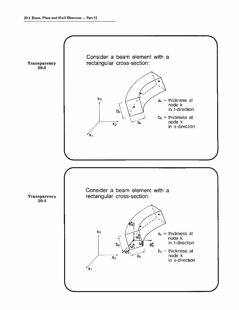
20-4 Beam, Plate and Shell Elements - Part II
Transparency20-3
Transparency20-4
Consider a beam element with arectangular cross-section:
ak = thickness atnode kin t-direction
bk = thickness atnode kin s-direction
Consider a beam element with arectangular cross-section:
ak = thickness atnode kin t-direction
bk = thickness atnode kin s-direction
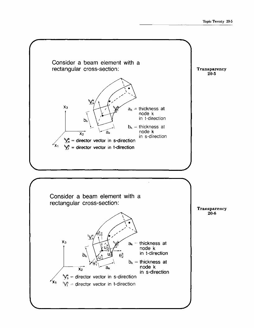
Topic Twenty 20-5
Consider a beam element with arectangular cross-section: Transparency
20-5
ak = thickness atnode kin t-direction
bk = thickness atnode kin s-direction
X2
t~ = director vector in s-directiont~ = director vector in t-direction
ak = thickness atnode kin t-direction
bk = thickness atnode kin s-direction
Consider a beam element with arectangular cross-section:
X2
t~~ = director vector in s-direction
t'i~ = director vector in t-direction
Transparency20-6

20-6 Beam, Plate and Shell Elements - Part II
where
tv~ = direction cosines of the directorvector in the t-direction, of nodek at time t
tV~i = direction cosines of the directorvector in the s-direction, of nodek at time t
The coordinates of the materialparticles of the beam are interpolated as
N Nt ~htk t~ htVkXi = ~ k Xi + 2 ~ ak k ti
k=1 k=1N
+ ~ k~1 bk hk tV~i
Transparency20-7
Transparency20-8
N t NtUi = }: hk tur + 2 }: ak hk CV~ - °V~)
k=1 k=1N
+ 2s L bk hk CV~i - °V~i)k=1
The vectors °V~ and °V~ can becalculated automatically from the initialgeometry of the beam element if theelement is assumed to lie initially in aplane.

Also
U. - t+dtX· - tx·1- I I
N t N S N
= ~ hk u~ + -2 ~ ak hk V~ + -2 ~ bk hk V~ik=1 k=1 k=1
where v~ and V~i are increments in thedirection cosines of the vectors tvr andtv~. These increments are given Tnterms of the incremental rotations ftk,about the Cartesian axes, as
Vr = ftk x tvr ; V~ = ftk X tv~
• Using the above displacement and geometryinterpolations, we can develop the straindisplacement matrices for the Cartesian straincomponents. A standard transformation yieldsthe strain-displacement relations correspondingto the beam coordinates TI, E, ,.
Topic 1\venty 20-7
Transparency20-9
Transparency20-10

2o-B Beam, Plate and Shell Elements - Part II
Transparency20-11
• The stress-strain relationship used forlinear elastic material conditions is
TJ~ TJ~ - components
o 0]Gk 0o Gk
Transparency20-12
k = shear correction factor
since only the one normal and twotransverse shear stresses are assumedto exist.
• The material stress-strain matrix foranalysis of elasto-plasticity or creepwould be obtained using also thecondition that only the stresscomponents (T1TJ) , (TJ~) and (TJ~) arenon-zero.

Topic 'I\venty 20-9
Transparency20-13
exact warpingdisplacementsfor squaresection
exact warpingdisplacementsfor infinitelynarrow section
• Note that the kinematic assumptions In thebeam element do not allow - so far - forcross-sectional out-of-plane displacements(warping). In torsional loading, allowing forwarping is important.
• We therefore amend the displacementassumptions by the following displacements:
t. u,
Torsion constant k in formula,T= k GO a3b
Transparency20-14
k
aAnalytical value
(Timoshenko) ADINA
1"02"04"0
10·0100"0
0'1410"2290"2810"3120'333
0"1410"2300"2890'3230"333

20-10 Beam, Plate and Shell Elements - Part II
Transparency20-15
Example: Twisting of a ring
All dimensions in inchesthickness = 0.2E=3 x 10⁵ psiv=0.3
0.2
Transparency20-16
Finite element mesh: Twelve 4-nodeiso-beam elements
4-nodeelement
ex prescribed

Topic 1\venty 20-11
DemonstrationPhotograph20-1Close-up of
;' ring deformations
Use the T.L. formulation to rotate the ring180 degrees: Transparency
20-17
Force-deflection curve
Moment(Ib-in)
50
25
O~------I----------i--
o 00 100
Rotation (degrees)

20-12 Beam, Plate and Shell Elements - Part II
Transparency20-18
Pictorially, for a rotation of 180 degrees,we have
Top view Side view
----- ........ ....'\
\\\
II
I/
//
/
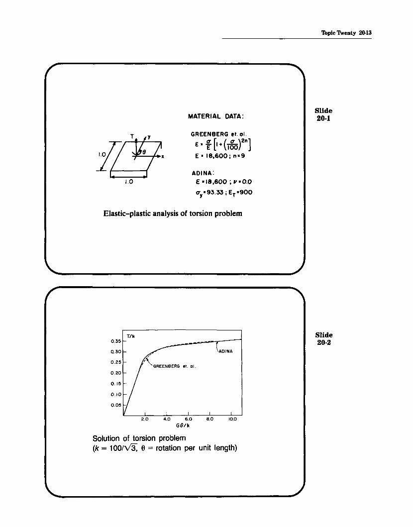
MATERIAL DATA:
GREENBERG et. a!.
E= [ [I + (lgo)2n]E = IB,600i n=9
ADINA:E =18,600; 11=0.0
CTy=93.33 i ET=900
'Ibpic Twenty 20-13
Slide20-1
Elastic-plastic analysis of torsion problem
T/k0.35
2.0 4.0 6.0G8/k
ADINA
10.0
Slide20-2
Solution of torsion problem(k = 1OO/~ 0 = rotation per unit length)

20-14 Beam, Plate and Shell Elements - Part II
Transparency20-19
Transparency20-20
Use of the isoparametric beam andshell elements
• The elements can be programmed foruse with different numbers of nodes- For the beam,
2, 3 or 4 nodes- For the shell,
4, 8, 9, "', 16 nodes
• The elements can be employed foranalysis of moderately thick structures(shear deformations are approximatelytaken into account).
• The elements can be used foranalysis of thin structures - but thenonly certain elements of thosementioned above should be used.
For shells: Use only the 16-nodeelement with 4 x 4 Gaussintegration over the mid-
X3 surface.
r
integration point

For beams:
Use 2-node beam element with 1-pointGauss integration along r-direction,
orUse 3-node beam element with 2-pointGauss integration along r-direction,
orUse 4-node beam element with 3-pointGauss integration along r-direction.
The reason is that the other elementsbecome overly (and artificially) stiffwhen used to model thin structures andcurved structures.
Two phenomena occur:
• Shear locking
• Membrane locking
Topic Twenty 20-15
Transparency20-21
Transparency20-22

20-16 Beam, Plate and Shell Elements - Part II
Transparency20-23
Transparency20-24
• The 2-, 3- and 4-node beamelements with 1-, 2- and 3-point Gaussintegration along the beam axes donot display these phenomena.
• The 16-node shell element with 4 x 4Gauss integration on the shell midsurface is relatively immune to shearand membrane locking (the elementshould not be distorted for bestpredictive capability).
• To explain shear locking, consider a2-node beam element with exactintegration (2-point Gauss integrationcorresponding to the r-direction).
r=-1 r=OTransverse displacement:
1 1w = 2" (1 - r) W1 + 2" (1 + r) W2
Section rotation:1 1
~ = 2" (1 - r) 61 + 2" (1 + r) 62

neutral axis7
I,
Hence the transverse shear deformationsare given· by
"Y=f~-~awax
x
Consider now the simple case of acantilever subjected to a tip bendingmoment, modeled using one 2-node
element:~. Ih pML
@16, = w, = 0 2)M
1Here 13 = "2 (1 + r) 62
1 1'Y = [w2 - "2 (1 + r) 92
Topic Twenty 20-17
Transparency20-25
Transparency20-26

20-18 Beam, Plate and Shell Elements - Part II
Transparency20-27
Transparency20-28
We observe:
• Clearly, 'Y cannot be zero at all pointsalong the beam, unless 62 and W2
are zero. But then also ~ would bezero and there would be no bendingof the beam.
• Since for the beam- bending strain energy oc: h3
- shear strain energy oc: hany error in the shear strains (due tothe finite element interpolationfunctions) becomes increasingly moredetrimental as h becomes small.
• For the cantilever example, theshear strain energy should be zero.As h decreases, the relative error inthe shear strain increases rapidlyand in effect, introduces an artificialstiffness that makes the model"lock."
h/L finite element solutionL = 100 Oanalytical (exact integration)
-9.6 x 10⁻⁷ 3.2 X 10-70.50
0.10 1.2 x 10⁻⁴ 2.4 X 10⁻⁶
0.01 1.2 x 10⁻¹ 2.4 X 10⁻⁵

• Although we considered only oneelement in the solution, the sameconclusion of locking holds for anassemblage of elements.
~ ••• \ ••••••• ?)Meach element should carrya constant bending moment
Example: Beam locking study
~ ......... JMn equally spaced elements
L=10 mSquare cross-section, height = 0.1 mTwo-node beam elements,full integration
Topic Twenty 20-19
Transparency20-29
Transparency20-30

20-20 Beam, Plate and Shell Elements - Part II
Transparency20-31
Plot tip deflection as a function of thenumber of elements:
32.00 Beam theory solution
10.008.006.004.002.00'10'
~Finiteelement solution(2-node beam elements,
full integration)
I~Height of element = Length of element
o+--;.I_.---...,.--~~--r---r--r----r----.-.o
8.00
24.00
16.00Tip
deflection(m)
Number of elements
Transparency20-32 Beam theory solution
0.3 1------------
Tipdeflection
(m)
0.2
0.1Finite element solution
\10 20 30
Number of elements

A remedy for the 2-node beam element is touse only 1-point Gauss integration (along thebeam axis).This corresponds to assuming a constanttransverse shear strain, (since the shear strainis only evaluated at the mid-point of the beam).
The bending energy is still integrated accurately
(since : is correctly evaluated).
h/L finite element solutionL = 100 6analytical (1-point integration)
0.50 9.6 x 10⁻⁷ 9.6 X 10⁻⁷
0.10 1.2 x 10⁻⁴ 1.2 X 10⁻⁴
0.01 1.2 x 10⁻¹ 1.2 X 10⁻¹
• The 3- and 4-node beam elements evaluatedusing 2- and 3-point integration are similarlyeffective.
• We should note that these beam elementsbased on "reduced" integration are reliablebecause they do not possess any spuriouszero energy modes. (They have only 6 zeroeigenvalues in 3-D analysis corresponding tothe 6 physical rigid body modes).
• The formulation can be interpreted as amixed interpolation of displacements andtransverse shear strains.
Topic Twenty 20-21
Transparency20-33
Transparency20-34

20-22 Beam, Plate and Shell Elements - Part II
Transparency20-35
Transparency20-36
• Regarding membrane-locking wenote that in addition to not exhibitingerroneous shear strains, the beammodel must also not contain erroneous mid-surface membrane strains inthe analysis of curved structures.
• The beam elements with reducedintegration also do not "membranelock~'
Consider the analysis of a curvedcantilever:

The exactly integrated 3-node beamelement, when curved, does containerroneous shear strains and erroneousmid-surface membrane strains. As aresult, when h becomes small, theelement becomes very stiff.
finite element finite elementsolution: 3-node solution: 3-node
h/R 9analytical element, 3-point element, 2-pointR = 100 (a = 45°) integration integration
0.50 7.5 x 10⁻⁷ 6.8 X 10⁻⁷ 7.4 X 10⁻⁷
0.10 9.4 x 10⁻⁵ 2.9 X 10⁻⁵ 9.4 X 10⁻⁵
0.01 9.4 x 10⁻² 4.1 X 10⁻⁴ 9.4 X 10⁻²
• Similarly, we can study the use of the4-node cubic beam element:
finite element finite elementh/R 9anaJytical solution: 4-node solution: 4-node
R = 100 (a = 45°) element, 4-point element, 3-pointintegration integration
0.50 7.5 x 10⁻⁷ 7.4 X 10⁻⁷ 7.4 X 10⁻⁷
0.10 9.4 x 10⁻⁵ 9.4 X 10⁻⁵ 9.4 X 10⁻⁵
0.01 9.4 x 10⁻² 9.4 X 10⁻² 9.4 X 10⁻²
We note that the cubic beam elementperforms well even when using fullintegration.
Topic Twenty 20-23
Transparency20-37
Transparency20-38

20-24 Beam, Plate and Shell Elements - Part II
Transparency20-39
Transparency20-40
Considering the analysis of shells, thephenomena of shear and membranelocking are also present, but thedifficulty is that simple "reduced"integration (as used for the beamelements) cannot be recommended,because the resulting elements containspurious zero energy modes.
For example, the 4-node shell elementwith 1-point integration contains 6spurious zero energy modes (twelvezero eigenvalues instead of only six).
Such spurious zero energy modes canlead to large errors in the solution that- unless a comparison with accurateresults is possible - are not known andhence the analysis is unreliable.

• For this reason, only the 16-nodeshell element with 4 x 4 Gaussintegration on the shell mid-surfacecan be recommended.
• The 16-node element should, asmuch as possible, be used with theinternal and boundary nodes placedat their ~rd points (without internalelement distortions). This way theelement performs best.
• Recently, we have developedelements based on the mixedinterpolation of tensorial components.
• The elements do not lock, in shear ormembrane action, and also do notcontain spurious zero energy modes.
• We will use the 4-node element,referred to as the MITC4 element, insome of our demonstrative samplesolutions.
Topic 1\venty 20-25
Transparency20-41
Transparency20-42

20-26 Beam, Plate and Shell Elements - Part II
Transparency20-43
The MITC4 element:
r
Transparency20-44
• For analysis of plates
• For analysis of moderately thickshells and thin shells
• The key step in the formulation is tointerpolate the geometry anddisplacements as earlier described,but
- To interpolate the transverse shearstrain tensor componentsseparately, with judiciously selectedshape functions
- To tie the intensities of thesecomponents to the valuesevaluated using the displacementinterpolations

rt transverse shear strain tensorcomponent interpolation
R?77,evaluated from
displacement interpolations
st transverse shear strain tensorcomponent interpolation
s
Topic Twenty 20-27
Transparency20-45
The MITC4 element
• has only six zero eigenvalues (nospurious zero energy modes)
• passes the patch test
What do we mean by the patch test?The key idea is that any arbitrarypatch of elements should be able torepresent constant stress conditions.
Transparency20-46

20-28 Beam, Plate and Shell Elements - Part II
THE PATCH TESTTransparency
20-47• We take an· arbitrary patch of
elements (some of which are geometrically distorted) and subjectthis patch to- the minimum displacementlrotn.
boundary conditions to eliminatethe physical rigid body modes,and
- constant boundary tractions,corresponding to the constantstress condition that is tested.
Transparency20-48 • We calculate all nodal point
displacements and element stresses.
The patch test is passed if the calculated element internal stresses andnodal point displacements are correct.

E=2.1 X 10⁶
v=0.3thickness = 0.01
.tX_2 (10,10)
r10
L_------..... (10,0)
(0,0) 1f-----10----.\ X1
PATCH OF ELEMENTS CONSIDERED
t
-0- 01
MEMBRANE TESTS
t
101 0 -0-!
BENDING/TWISTING TESTS
Topic 1\venty 20-29
Transparency20-49
Transparency20-50

20·30 Beam, Plate and Shell Elements - Part II
Transparency20-51
Example: Spherical shell
radius = 10.0thickness = 0.04E=6.825x 10⁷
v=0.3
Transparency20-52
Selection of director vectors:• One director vector is generated
for each node.
• The director vector for each nodeis chosen to be parallel to theradial vector for the node.
• In two dimensions:
vector
~-------x
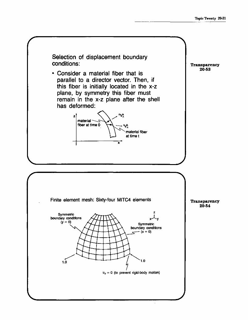
Selection of displacement boundaryconditions:
• Consider a material fiber that isparallel to a director vector. Then, ifthis fiber is initially located in the x-zplane, by symmetry this fiber mustremain in the x-z plane after the shellhas deformed:
Topic 1\venty 20-31
Transparency20-53
zmaterial ~ .,-......fiber at time 0 _tv~
material fiberat time t
x
Finite element mesh: Sixty-four MITC4 elements Transparency20-54
Symmetricboundary conditions
(y = 0)
~
/1.0
z
xAySymmetric
boundary conditions~(x=O)
Uz = 0 (to prevent rigid-body motion)

20-32 Beam, Plate and Shell Elements - Part II
Transparency20-55
This condition is applied to each nodeon the x-z plane as follows:
z
Transparency20-56
• A similar condition is applied tonodes initially in the y-z plane.
• These boundary conditions aremost easily applied by makingeuch node in the x-z or y-zplane a 6 degree of freedomnode. All other nodes are 5degree of freedom nodes.
• To prevent rigid body translationsin the z-direction, the z displacement of one node must be setto zero.

zL y
Linear elastic analysis results:
• Displacement at point of loadapplication is 0.0936 (analyticalsolution is 0.094).
• Pictorially,
Exam~: Analysis of an open (five-sided)box:
Box is placed open-side-down/Add on africtionless surface.~ Uniform pressure
Box is modeledusing shellelements
rigid,frictionlesssurface
Topic 1\venty 20-33
Transparency20-57
Transparency20-58

20-34 Beam, Plate and Shell Elements - Part II
Transparency20-59
Modeling of the box with shellelements:
- Choose initial director vectors.
- Choose 5 or 6 degrees of freedomfor each node.
- Choose boundary conditions.
Transparency20-60
- Instead of input of director vectors,one for each node, it can be moreeffective to have ADINA generatemid-surface normal vectors.
- If no director vector is input for anode, ADINA generates for eachelement connected to the node anodal point mid-surface normalvector at that node (from theelement geometry).
- Hence, there will then be as manydifferent nodal point mid-surfacenormal vectors at that node asthere are elements connected tothe node (unless the surface isflat).

Nodal point mid-surface normal vectors for the box:
- We use the option of automatic generation ofelement nodal point mid-surface normal vectors.
- At a node, not on an edge, the result is onemid-surface normal vector (because the surfaceis flat).
- At an edge where two shell elements meet,two mid-surface normal vectors are generated(one for each element). ---s:;-- one mid-surface
normal vectorused at this node
two mid-surfacenormal vectorsused at this node
Degrees of freedom:
Topic Twenty 20-35
Transparency20-61
Transparency20-62
6 degreesof freedom no rotational
stiffness forthis degreeof freedom

20-36 Beam, Plate and Shell Elements - Part II
Note added in preparation ojstudy-guideIn the new version of ADINA (ADINA 84 with an update inserted, or ADINA 86)
the use of the 5 or 6 shell degree of freedom option has been considerably automatized:- The user specifies whether the program is to use 5 or 6 degrees of freedom at each
shell mid-surface node NIGL(N).EQ.O-6 d.o.f. with the translations and rotations corresponding to the
global (or nodal skew) systemIGL(N).EQ.l-+5 d.o.f. with the translations corresponding to the global (or nodal
skew) system but the rotations corresponding to the vectors VIand V2
- The user (usually) does not input any mid-surface normal or director vectors. Theprogram calculates these automatically from the element mid-surface geometries.
- The user recognizes that a shell element has no nodal stiffness corresponding tothe rotation about the mid-surface normal or director vector. Hence, a shell midsurface node is assigned 5 d.o.f. unless
a shell intersection is considereda beam with 6 d.o.f. is coupled to the shell nodea rotational boundary condition corresponding to a global (or skew) axis is to beimposeda rigid link is coupled to the shell node
For further explanations, see the ADINA 86 users manual.
-: admissible-*-: deleted
Displacement boundary conditions:Box is shown open-side-up.
f
+representative nodenot at a corner
Transparency20-63

Consider a linear elastic static analysisof the box when a uniform pressureload is applied to the top.We use the 128 element mesh shown(note that all hidden lines are removedin the figure): lv
x
4-nodeshellelement
We obtain the result shown below(again the hidden lines are removed):
• The displacements in this plot arehighly magnified.
Topic 1\venty 20-37
Transparency20-64
Transparency20-65
z
~vx

20-38 Beam, Plate and Shell Elements - Part II
Slide20-3
o
.,. ERROR -5IN CENTER
DISPLACFMENT
-10
-15
.--~II "Q3 L[Eg:• N"2
I--
2N
4 6
Slide20-4
Simply-supported plate under uniform pressure,Uh = 1000
o11~t==t==+====t====t1
Of. ERROR -51---+---+---...,1---+---+--+----1IN CENTER
OISPLACEMENT
-101---+---+---+--+---+---+--1
-15 L...-_....L..._~_--J,__~_....L..._......I.._---1
2 N 4 6
Simply-supported plate under concentrated loadat center, Uh = 1000

o
.,. ERROR -5IN CENTER
DISPLACEMENT
-10
-15
~~
Thpic 1\venty 20-39
Slide20-5
2N
4 6
Clamped plate under uniform pressure, Uh = 1000
~-~
~
V/
/
o
"to ERROR -5IN CENTER
DISPLACEMENT
-10
-152
N4 6
Slide20-6
Clamped plate under concentrated load atcenter. Uh = 1000
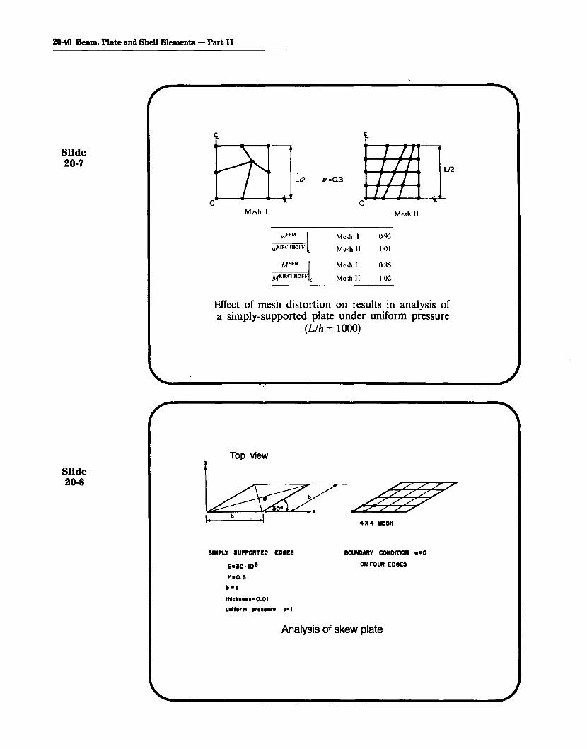
20-40 Beam, Plate and Shell Elements - Part II
Slide20-7
Mesh I
/I =0.3
Mesh 1\
M~"M IMKIRClIIIOI.".' C
Mesh I
Mesh II
Mesh I
Mesh"
0·93
Hli
0.85
1.02
Slide20-8
Effect of mesh distortion on results in analysis ofa simply-supported plate under uniform pressure
(L/h = 10(0)
Top viewr
SIMPLY SUPPORTED EDIES
E.50 0 10·
~"'0.5
b .1
thickn...·O.OI
unlf.'1Il pr•••ur. p"'1
IlOUNDARY CONDmON ••0
ON FOUR EDGES
Analysis of skew plate

MESH .FEM;' MO FEM~ MO FEM AMOe ·e Mmax Mmax Mmln Mmln
4X4 0.879 0.873 0.852
8X8 0.871 0.928 0.922
16X 16 0.933 0.961 0.919
32X32 0.985 0.989 0.990
Solution of skew plate at point C usinguniform skew mesh
2 X 2 MESH
MESH FEM/ wMO FEM/ MO FEM/ MO"c c Mmox Mmex Mmm Mmm
2X2 0.984 0.717 0.602
4 X4 0.994 0.935 0.878
Solution of skew plate using a more effective mesh
Topic Twenty 20-41
Slide20-9
Slide20·10

20-42 Beam, Plate and Shell Elements - Part II
Slide20-11
11----- L ----.I/-r
TL = 12 INI = 1/12 IN 4
A = I IN2
E = 3.0x 10⁷
PSI11= 0M = CONC E NTRATE D
END MOMENT
Large displacement analysis of a cantilever
1.0
Slide20-12
RATIOS
u/L, oIL, </>/2"
0.2
0.4 0.5MOMENT PARAMETER '1 = ML/2"E I
Response of cantilever

1.0__ ANALYT. SOLN.
u 0.8Lv w/L
Vw 0.6 V
L Z 7L
v.
<t>9J o u/L
211'
TWO 4-NODE ELEMENT MODEL
ML27i'IT'
Large displdcement/rotation analysis of acanti 1ever
Topic 'l\venty 20-43
Slide20-13
Slide20-14
~ 0.6LZZ7THREE 4- NODE ELEMENT MODEL
..ILL 08
V w/Lv.
v.
0.1 0.2 0.3
ML27rEI

20-44 Beam, Plate and Shell Elements - Part II
MATERIAL DATA:
Slide E 30 , 10' psi
20-15"
0 0.3
E 0 0.0T
Z a 0 30 '10 3 psiy
...!1D'IN
T 0.91N
iOi'N1,0 IN
Analysis of I-beam
Slide20-16
- FREE END
Iso-beam model

Shell model
Topic 1\venty 20-45
Slide20-17
y
..-:
,
f-- -xT
_".~~
----8. Z
y
Slide20-18
I--- 50 IN---lI- --IO.OIN---I
I-beam

2046 Beam, Plate and Shell Elements - Part II
~SO-beammodel
MERCHANT'SUPPER BOUND
"SAND HEAP"~
;Shellmodel
.-....&._--------~
200
100
300
T IN-LBS
Slide20-19
o 0.10 020 0.308. RADIANS
0.40
Rotation of I-beam about X -axis for increasingtorsional moment.
Slide20-20
IXI UNI'ORM MESH USEDTO REPRESENT AREA ABCD
E =21,0001/=0
Er O
aY=4.2
L 0:15,200
R 0: 7,600
1/)= 40
fhickn.u=76
Large deflection elastic-plastic analysis of a cylindrical shell

2
o Kr8keland
-MITC4
4 POINT GAUSS INTEGRATIONTHROUGH ELEMENT THICKNESS
50 100 150 200
we
Response of shell
Topic 1\venty 20-47
Slide20-21

Contents:
Textbook:
References:
Topic 21
A DemonstrativeComputer SessionUsing ADINALinear Analysis
• Use of the computer program ADINA for finite elementanalysis, discussion of data preparation, programsolution, and display of results
• Capabilities of ADINA
• Computer laboratory demonstration-Part I
• Linear analysis of a plate with a hole for the stressconcentration factor
• Data input preparation and mesh generation
• Solution of the model
• Study and evaluation of results using plots of stresses,stress jumps, and pressure bands
Appendix
The use of the ADINA program is described and sample solutions aregiven in
Bathe, K. J., "Finite Elements in CAD - and ADINA," NuclearEngineering and Design, to appear.
ADINA, ADINAT, ADINA-IN, and ADINA-PLOT Users Manuals,ADINA Verification Manual, and ADINA Theory and Modeling Guide,ADINA Engineering, Inc., Watertown, MA 02172, U.S.A.
Proceeding~ of the ADINA Conferences, (Bathe, K. J., ed.)Computers & Structures
13, 5-6, 198117, 5-6, 198321, 1-2, 1985

21-2 Computer Session Using ADINA - Linear Analysis
References: The use of pressure band plots to evaluate meshes is discussed in (continued) Sussman, T., and K. J. Bathe, "Studies of Finite Element Procedures
Stress Band Plots and the Evaluation of Finite Element Meshes," Engineering Computations, to appear.

A FINITE ELEMENTANALYSIS - LINEAR
SOLUTION• We have presented a considerable
amount of theory and example solution results in the lectures.
• The objective in the next two lectures is to show how an actual finiteelement analysis is performed on thecomputer.
• We cannot discuss in detail all theaspects of the analysis, but shallsummarize and demonstrate on thecomputer the major steps of theanalysis, and concentrate on
- possible difficulties- possible pitfalls- general recommendations
Topic Twenty-one 21-3
Transparency21-1
Transparency21-2

21-4 Computer Session Using ADINA - Linear Analysis
Transparency21-3 We will use as the example problem
the plate with a hole already considered earlier, and perform linear andnonlinear analyses
elastic analysis to obtain thestress concentration factorelasto-plastic analysis to estimatethe limit loadan analysis to investigate the effectof a shaft in the plate hole
Plate with hole: Schematic drawing
Transparency21-4
1 E = 207000 MPaj-----:.---+777Jjrim~ v = 0.3
thickness = 0.01 m
plane stressconditions
:-:~~~t'"We consider thisquarter of the---+ plate and
use symmetryconditions
0.01m-+-_.J
0.1m
I. 0.1m,I

• The first step for a finite elementanalysis is to select a computer program. We use the ADINA system.
ADINA-IN to prepare, generatethe finite elementdata
ADINA to solve the finiteelement model
ADINA-PLOT to display numeri-cally or graphicallythe solution results
Schematically:
graphics..>display
terminal
User work-station
Topic 1\venty-one 21-5
Transparency21-5
Transparency21-6

21-6 Computer Session Using ADINA - Linear Analysis
Transparency21-7
I I generatedUser - ADINA-IN - ADINA
input file
• User types into terminal ADINA-INcommands interactively or for batchmode processing. User checks inputand generated data on graphicsdisplay terminal.
Transparency21-8
• ADINA-IN generates the input datafor ADINA.
• The input data is checked internallyin ADINA-IN for errors and consistency and is displayed as perrequest by the user.
• The degree of freedom numbers aregenerated (for a minimum bandwidth).

--I ADINA
Topic 1\ventyo()ne 21-7
Transparency21-9
• User runs ADINA to calculate theresponse of the finite elementmodel. ADINA writes the model dataand calculated results on an outputfile and stores the model data andcalculated results on the portholefile.
ADINA-PLOT I~
User _--;1display outputdata, numericallyor graphically
Transparency21-10
• User runs ADINA-PLOT to accessthe output data and display selectedresults; displacements, stresses,mode shapes, maxima, ...
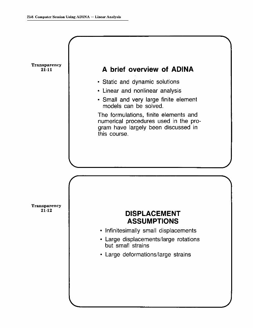
21-8 Computer Session Using ADINA - Linear Analysis
Transparency21-11
Transparency21-12
A brief overview of ADINA
• Static and dynamic solutions
• Linear and nonlinear analysis
• Small and very large finite elementmodels can be solved.
The formulations, finite elements andnumerical procedures used in the program have largely been discussed inthis course.
DISPLACEMENTASSUMPTIONS
• Infinitesimally small displacements
• Large displacements/large rotationsbut small strains
• Large deformations/large strains
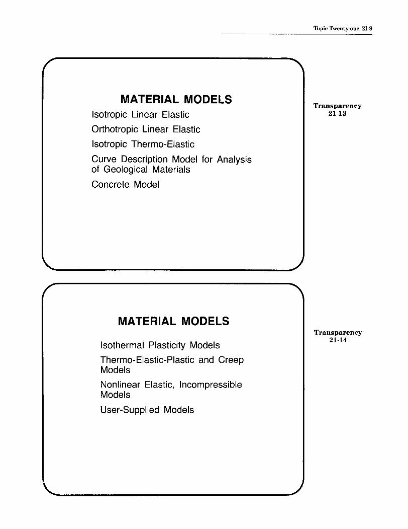
MATERIAL MODELSIsotropic Linear Elastic
Orthotropic Linear Elastic
Isotropic Thermo-Elastic
Curve Description Model for Analysisof Geological Materials
Concrete Model
MATERIAL MODELS
Isothermal Plasticity Models
Thermo-Elastic-Plastic and CreepModels
Nonlinear Elastic, IncompressibleModels
User-Supplied Models
Topic Twenty-one 21-9
Transparency21-13
Transparency21-14
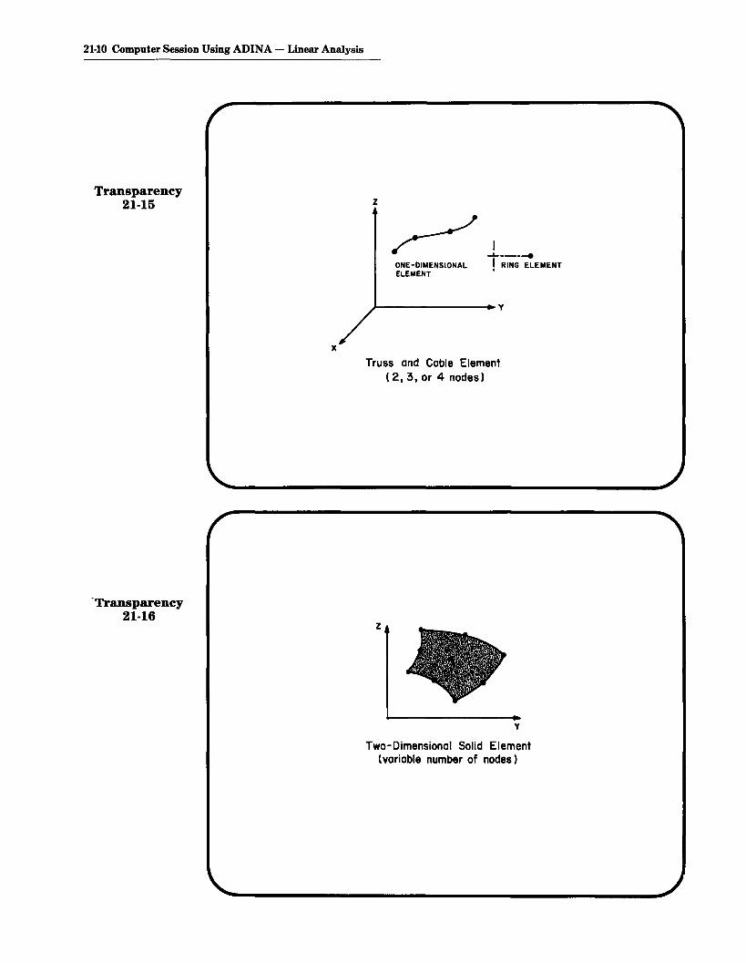
21-10 Computer Session Using ADINA - Linear Analysis
Transparency21-15 z
ONE-DIMENSIONALELEMENT
I......-.-! RING ELEMENT
x
r-------.... v
Truss and Cable Element(2,3, or 4 nodes)
Transparency21-16
z
v
Two-Dimensional Solid Element(variable number of nodes)

z
x
y
z
)(
Three-Dimensional Solid Element(variable number of nodes I
y
Two-Node Beam Element
Topic 1\ventY'one 21-11
Transparency21-17
Transparency21-18

21-12 Computer Session Using ADINA - Linear Analysis
Transparency21-19
z
/
r----V
x
Isoparametric Beam Element(2,3,4 nodes)
Transparency21-20
z
AT EACH NODE 6 BEAMDEGREES OF FREEDOMPLUS OVALIZATION
~-----v DEGREES OF FREEDOMx
Pipe Element with Ovalization

16 Node Element
}-,x
4 Node Element
ELEMENTS ARE USED WITH5 OR 6 DEGREES OFFREEDOM PER NODE
Topic 1\venty-one 21-13
Transparency21-21
Plate and Shell Elements
A SUMMARY OF IMPORTANTOBSERVATIONS
• We need to check the finite elementdata input carefully
prior to the actual responsesolution run, andafter the response solution hasbeen obtained by studyingwhether the desired boundaryconditions are satisfied, whetherthe displacement and stresssolution is reasonable (for thedesired analysis).
Transparency21-22

21-14 Computer Session Using ADINA - Linear Analysis
Transparency21-23
Transparency21-24
• We need to carefully evaluate andinterpret the calculated response
study in detail the calculated displacements and stresses alongcertain lines, study stress jumps
stress averaging, stress smoothing should only be done after theabove careful evaluation
Data for Construction of64 Element Mesh:
100 MPa
E = 207,000 MPav = 0.3Plane stressthickness = 0.01 m

Finite element mesh to be generatedusing ADINA-IN:
• Mesh contains 64 elements,288 nodes.
Topic Twenty-one 21-15
Transparency21-25
eight-nodeisoparametricelement
DemonstrationPhotograph
21-1Finite Element Research
Group Laboratorycomputer configuration
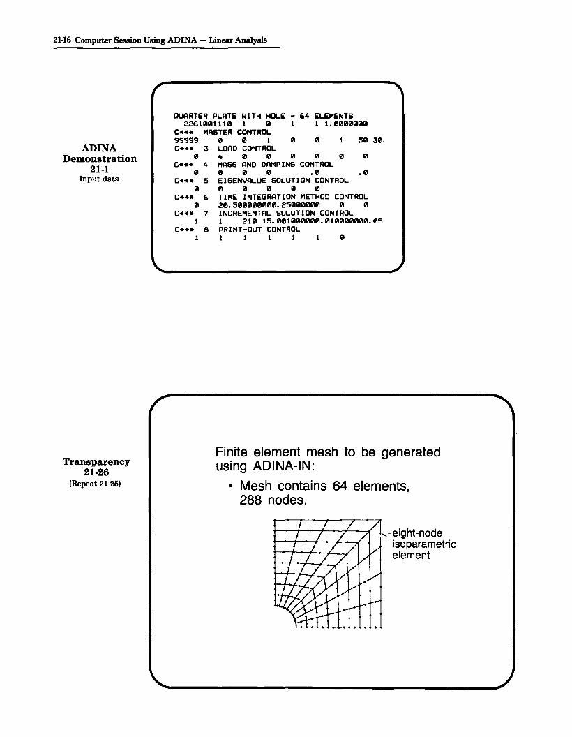
21-16 Computer Session Using ADINA - Linear Analysis
ADINADemonstration
21-1Input data
Transparency21-26
(Repeat 21-25)
QUARTER PLATE WITH HOLE - 64 ELEMENTS2261001110 1 0 1 1 1.0000000
C... MASTER CONTROL99999 0 0 1 0 0 50 30.C••* 3 LOAD CONTROL
o 4 0 0 0 0 0 0C*.* 4 MASS AND DAMPING CONTROL
o 0 0 0 .0 .0C••* 5 EIGENVALUE SOLUTION CONTROL
o 0 0 0 0 0C... 6 TIME INTEGRATION METHOD CONTROL
o 20.500000000.25000000 0 0C••* 7 INCREMENTAL SOLUTION CONTROL
1 1 210 15.001000000.010000000.05C.*. 8 PRINT-OUT CONTROL
11111 0
Finite element mesh to be generatedusing ADINA-IN:
• Mesh contains 64 elements,288 nodes.
eight-nodeisoparametricelement

Stress vector output: Example
Topic Twenty-one 21-17
Transparency21-27
integrationpoint ~
/ maximum principal stress,/----' (tensile)
minimum principal stress(compressive)
The length of the line is proportionalto the magnitude of the stress.
TIME 1.000 DMAX ,300
ADINADemonstration
21-2Deformed meshplot

21-18 Computer Session Using ADINA - Linear Analysis
Plate with hole: Schematic drawing
Transparency21-28
0.1m
0.01 m--+----./
0.1m.1
E = 207000 MPav =0.3
thickness = 0.01 m
We consider thisquarter of theplate anduse symmetryconditions
plane stressconditions
Transparency21-29
(Repeat 21-25)
Finite element mesh to be generatedusing ADINA-IN:
• Mesh contains 64 elements,288 nodes.
~eight-node
isoparametricelement

s-- stress computed at closestintegration point
Stress point numbers and integrationpoint numbers for element 57
2 integrationpoint
6 3X
2X
3 1 6 5x 5 X4 X
7x
987 X Xx4
P 8stress point
Behavior of stresses near the stressconcentration:
radius(J of s- stress computed at nodal point
hole
length of element
Topic Twenty-one 21-19
Transparency21·30
Transparency21-31
distance z = 0
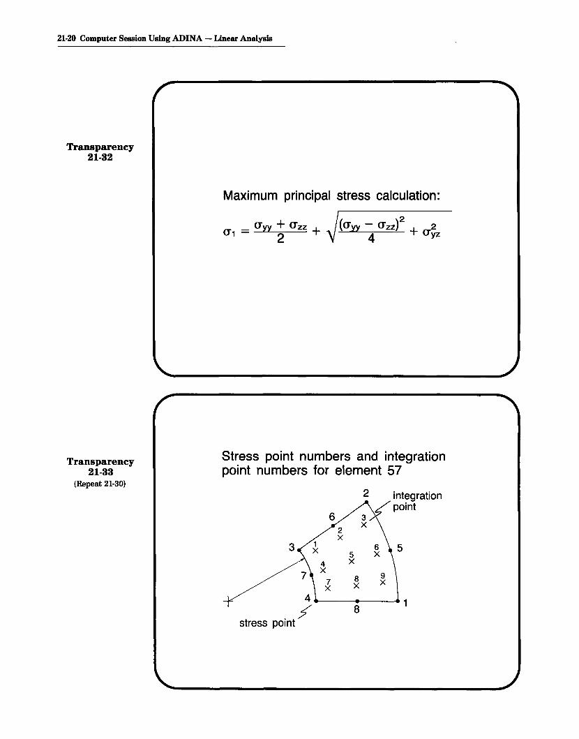
21-20 Computer Session Using ADINA - Linear Analysis
Transparency21-32
Maximum principal stress calculation:
_ {1yy + {1zz + !({1yy - {1ZZ)2 + 2{11 - 2 -V. 4 {1yz
Transparency21-33
(Repeat 21-30)
Stress point numbers and integrationpoint numbers for element 57
integrationpoint
2
62X
5X
8 9X x
8
3
4--_~t-------1
.:5stress POint

RESULTANT • SMAX ARITHMETIC EXPRESSION.
Topic Twenty-one 21-21
lTVV+TZZI ITWO+SllRT IITVV-TZZ) * lTVV-TZZ) IFDUR+TVZHVZ I
EXTREME ELEMENT RESULTS PER ELEMENT GROUP FOR WHOLE MODEL
TVV • VV-STRESSTZZ • ZZ-STRESSTVZ • VZ-STRESSTWO • 2.1Il1ll1ll00FOUR • 4.1Il1ll1ll1ll1ll
INTERVAL TSTART- 1.1Il1ll1ll1ll TEND= 1. 0000 SCANNED FOR ABSOLUTE MAXIMUM
ADINADemonstration
21-3Close-up ofcalculations
ELEMENT BROUP NO. 1 (2-D SOLID) LISTED RESULTS ARE MEASURED INGLOBAL COORD I NATE SYSTEM
RESULTANT SMAX ELEMENT POINT TIME STEP
Ill. 34~ISIE+1Il3 ~7 4 Ill. 1IIlIIlIllIllE+1Il1
Finite element mesh to be generatedusing ADINA-IN:
• Mesh contains 64 elements,288 nodes.
Transparency21-34
(Repeat 21-25)
eight-nodeisoparametricelement

21-22 Computer Session Using ADINA - Linear Analysis
Transparency21-35
(Repeat 2-33)
Transparency21-36
(Repeat 2-35)
• To be confident that the stressdiscontinuities are small everywhere,we should plot stress jumps along eachline in the mesh.
• An alternative way of presentingstress discontinuities is by means ofa pressure band plot:- Plot bands of constant pressure
where
pressure = - (Txx + ; yy + Tzz)
Sixty-four element mesh: Pressure bandplot
H~5 MPa 5 MPa

A SUMMARY OF IMPORTANTOBSERVATIONS
• We need to check the finite elementdata input carefully
- prior to the actual responsesolution run, and
- after the response solution hasbeen obtained by studyingwhether the desired boundaryconditions are satisfied, whetherthe displacement and stresssolution is reasonable (for thedesired analysis).
Topic 1\venty-one 21-23
ADINADemonstration
21-4Close-up of
pressure bands
. Transparency21-37
(Repeat 21-221

21-24 Computer Session Using ADINA - Linear Analysis
Transparency21·38
(Repeat 21-23) • We need to carefully evaluate andinterpret the calculated response
study in detail the calculated displacements and stresses alongcertain lines, study stress jumps
stress averaging, stress smoothing should only be done after theabove careful evaluation

Contents:
Textbook:
References:
Topic 22
A DemonstrativeComputer SessionUsing ADINA-Nonlinear Analysis
• Use of ADINA for elastic-plastic analysis of a plate witha hole
• Computer laboratory demonstration-Part II
• Selection of solution parameters and input datapreparation
• Study of the effect of using different kinematicassumptions (small or large strains) in the finite elementsolution
• Effect of a shaft in the plate hole, assuming frictionlesscontact
• Effect of expanding shaft
• Study and evaluation of solution results
Appendix
The use of the ADINA program is described and sample solutions aregiven in
Bathe, K. J., "Finite Elements in CAD - and ADINA," NuclearEngineering and Design, to appear.
ADINA, ADINAT, ADINA-IN, and ADINA-PLOT Users Manuals,ADINA Verification Manual, and ADINA Theory and Modeling Guide,ADINA Engineering, Inc., Watertown, MA 02172, U.S.A.

22-2 Computer Session Using ADINA - Nonlinear Analysis
References:(continued)
Proceedings of the ADINA Conferences, (K. J. Bathe, ed.)Computers & Structures
13, No. 5-6, 198117, No. 5-6, 198321, No. 1-2, 1985
The contact solution procedure used in the analysis of the plate withthe shaft is described in
Bathe, K. J., and A. Chaudhary, "A Solution Method for Planar andAxisymmetric Contact Problems," International Journal for Numerical Methods in Engineering, 21, 65-88, 1985.

Topic 'l\venty-two 22-3
A FINITE ELEMENTANALYSIS - NONLINEAR
SOLUTION• We continue to consider the plate
with a hole.
• A nonlinear analysis should only beperformed once a linear solution hasbeen obtained.The linear solution checks the finiteelement model and yields valuableinsight into what nonlinearities mightbe important.
Transparency22-1
Plate with hole: Schematic drawing
Transparency22-2
(Repeat 21-4)
plane stressconditions
r////J'///'/J'///71""'-""'We consider thisquarter of theplate anduse symmetryconditions
1 E = 207000 MPar-~---f-7"TTn7-rrT77777I v = 0.3
thickness = 0.01 m
0.01m-+--.../
0.1m
I.0.1m
.1

22-4 Computer Session Using ADINA - Nonlinear Analysis
Transparency22-3
(Repeat 21-25)
Finite element mesh to be generatedusing ADINA-IN:
• Mesh contains 64 elements,288 nodes.
eight-nodeisoparametricelement
Transparency22-4
• Some important considerations arenow
What material model to selectWhat displacement/strainassumption to makeWhat sequence of load application to chooseWhat nonlinear equation solutionstrategy and convergence criteriato select

• We use the ADINA system toanalyse the plate for its elastoplastic static response.
• We also investigate the effect onthe response when a shaft isplaced in the plate hole.
Some important observations:• The recommendations given in the
linear analysis are here also applicable (see previous lecture).
• For the nonlinear analysis we needto, in addition, be careful with the
- sequence and incrementalmagnitudes of load application
- choice of convergence tolerances
Topic Twenty-two 22·5
Transparency22-5
Transparency22-6

22-6 Computer Session Using ADINA - Nonlinear Analysis
Transparency22-7
Transparency22-8
Limit load calculations:
p
rTTTTl
o
LL..LLLJp
• Plate is elasto-plastic.
Elasto-plastic analysis:
Material properties (steel)(T
740 -I--
(T
(MPa)~
ET = 2070 MPa, isotropic hardening
E = 207000 MPa, v = 0.3
e• This is an idealization, probably
inaccurate for large strain conditions(e > 2%).

Load history:
650+---------++
Topic 1\venty·two 22·7
Transparency22-9
Load(MPa)
13 14 time
• Load is increased 50 MPa per load step.
• Load is released in one load step.
USER-SUPPLIED
MATERHlL 1 PLASTIC E=207000 NU=0.3 ET=2070 YIELD=740MATERIAL 1 PLASTIC E=207000 NU=0.3 ET=2070 YIELD=740DELETE EQUILIBRIUM-ITERATIONSDELETE EQUILIBRIUM-ITERATIONSADINAADINA
ADINADemonstration
22-1Input data

22-8 Computer Session Using ADINA - Nonlinear Analysis
Transparency22-10
(Repeat 21-25)
Finite element mesh to be generatedusing ADINA-IN:
• Mesh contains 64 elements,288 nodes.
eight-nodeisoparametricelement
Transparency22-11
Load history:
650-+-------~+
Load(MPa)
o~-------+-+---
o 13 14 time
• Load is increased 50 MPa per load step.
• Load is released in one load step.
• The BFGS method is employed for each load step.

Convergence criteria:
Energy:
d1!(i)T [t+~tB _ t+~tE(i-1)] < =
dU(1)T[t+~tR _ tF] - ETOl 0.001
Force:Ilt+~tR _ t+~tF(i-1)112 < _
RNORM - RTOl - 0.01
(RNORM = 100 MPa x 0.05 m x 0.01 m)~~~
nominal width thicknessappliedload
Topic Twenty-two 22-9
Transparency22-12
ADINADemonstration
22-2Plot of plasticityin plate with hole

22·10 Computer Session Using ADINA - Nonlinear Analysis
Transparency22-13
Stress vector output: Example
integrationpoint ~
/ maximum principal stress/ .....-" (tensile)
-s-- minimum principal stress(compressive)
ADINADemonstration
22-3Close-up of stress
vectors around hole
The length of the line is proportionalto the magnitude of the stress.
ORIQ:tNAL _ BSCALE '987. A

Finite element mesh to be generatedusing ADINA-IN:
• Mesh contains 64 elements,288 nodes.
Topic 1\venty-two 22-11
Transparency22-14
(Repeat 21-25)
eight-nodeisoparametricelement
M.N.O. Materially-Nonlinear-Only analysis
T.L. Total Lagrangianformulation
U.L. Updated Lagrangianformulation
Transparency22-15
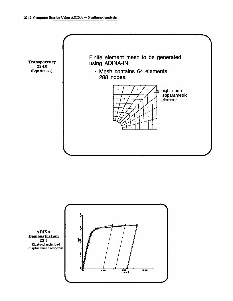
22-12 Computer Session Using ADINA - Nonlinear Analysis
Transparency22-16
(Repeat 21-25)
Finite element mesh to be generatedusing ADINA-IN:
• Mesh contains 64 elements,288 nodes.
ADINADemonstration
22-4Elasto-plastic load
displacement response
I•
III
I..
eight-nodeisoparametricelement

100 MPa
rTTTTlPlate with shaft:
plate, /E = 207000 MPav=0.3thickness = 0.01 mplane stress
conditions
long shaft,E = 207000 MPa
b v =0.3~ thickness=0.05 m
_~ plane strain., conditions
Topic Twenty-two 22-13
Transparency22-17
LLLLLJ100 MPa
• The shaft is initially flush with the hole.
• We assume no friction between the shaft andthe hole.
Detail of shaft:
shaft .J(collapsed 8-node
elements)
Transparency22-18

22-14 Computer Session Using ADINA - Nonlinear Analysis
Transparency22-19
ADINADemonstration
22-5Deformed mesh
Solution procedure: Full Newtoniterations withoutline searches
Convergence criteria:
Energy: ETOL = 0.001
Force: RTOL = 0.01 , RNORM = 0.05 N
Incremental contact force:
IILiB(i-1) -: LiB(i-2)112 < =IILiR(,-1)112 - RCTOL 0.05
DEFORMED _ DSCALE 18641TU1E 1.888 DtlAX .388

Plate with expanding shaft:
Topic Twenty-two 22-15
Elasto-plasticplate ~
100 MPa
rTTTn/Shaft
./
~100 MPa
Transparency22-20
• The shaft now uniformly expands.
ADINADemonstration
22-6Close-up of
deformations atcontact

Contents:
Glossary
Glossaryof Symbols
• Glossary of Roman Symbols
• Glossary of Greek Symbols

Glossary of Roman Symbols
Glossary G-l
IA
C
Cjj
The Euclidean norm or "two-norm. "For a vector a
1@l12 = ~f. (8k)2
When used above a symbol, denotes"in the rotated coordinate system."
Cross-sectional dimensions of a beamat nodal point k.
Cross-sectional area at time t.
A square matrix used in the BFGSmethod.
Linear strain-displacement matrixused in linear or M.N.O. analysis.
Linear strain-displacement matrixused in the T.L. formulation.
Linear strain-displacement matrixused in the D.L. formulation.
Intermediate matrices used to compute hBl; hBll contains the "initialdisplacement effect."
Nonlinear strain-displacement matrix used in the T.L. formulation.
Nonlinear strain-displacement matrix used in the D.L. formulation.
The wave speed of a stress wave(dynamic analysis).
Diagonal element corresponding to theith degree of freedom in the dampingmatrix (dynamic analysis).
The damping matrix (dynamicanalysis).
c
CEPiJ's
oCijrS
ONORM
OMNORM
OTOL
The Mooney-Rivlin material constants (for rubberlike materials).
Components of the Cauchy-Greendeformation tensor (basic concepts ofLagrangian continuum mechanics).
Matrix containing components of theconstitutive tensor referred to a localcoordinate system.
Matrix containing components of theconstitutive tensor, used in linear andM.N.O. analysis.
Matrix containing components of theconstitutive tensor oeyrs ,used in the T.L. formulation.
Matrix containing components of theconstitutive tensor tCyrs •used in the D.L. formulation.
Components of elastic constitutive tensor relating d<Ji~ to de~
Components of elasto-plastic constitutive tensor relating d<J, to ders
Components of tangent constitutivetensor relating doS t to doErs
Components of tangent constitutivetensor relating dlSt to dlE rs
Reference displacement used withdisplacement convergence toleranceDTOL (solution of nonlinearequations).DMNORM is the reference rotationused when rotational degrees offreedom are present.
Convergence tolerance used to measure convergence of the displacements and rotations (solution of nonlinear equations).

G-2 Glossary
det The determinant function, forexample, det J~ .
Strain hardening modulus (elastoplastic analysis).
'dV A differential element of volumeevaluated at time t.
A differential element of volumeevaluated at time O.
Vector describing the 6rientation andlength of a differential material fiber attime t (basic concepts of Lagrangiancontinuum mechanics).
ETOL
f(x)
Convergence tolerance used to measure convergence in energy (solutionof nonlinear equations).
A function that depends on X(solution of nonlinear equations).
A vector function that depends onthe column vector U(solution of nonlinear equations).
Vector describing the orientation andlength of a differential material fiberat time 0 (basic concepts of Lagrangiancontinuum mechanics).
IfF, IfF Components of externally appliedforces per unit current volume and unitcurrent surface area.
Effective creep strain, evaluated attime t (creep analysis).
IF Yield function (elasto-plastic analysis).
Components of infinitesimal strain tensor (linear and M.N.O. analysis).
IE Vector of nodal point forces equivalent to the internal element stresses.
inelasticcreepplasticthermalviscoplastic
Unit vectors in the r, S, and t directions (shell analysis).
Linear (in the incremental displacements) part of oE;;.(T.L. formulation)
Vector of nodal point forces equivalent to the internal element stresses(T.L. formulation).
Column vector containing the inertiaforces for all degrees of freedom(dynamic analysis).
Column vector containing the elasticforces (nodal point forces equivalentto element stresses) for all degreesof freedom (dynamic analysis).
Acceleration due to gravity.
Column vector containing the damping forces for all degrees of freedom(dynamic analysis).
Vector of nodal point forces equivalent to the internal element stresses(U.L. formulation).
9
JE
Ee(t)
Eo(t)
of inelastic strainstime t (inelastic
Linear (in the incremental displacements) part of IE;;.
(U.L. formulation).
Various typesevaluated atanalysis):
IN
cP
THVP
Ie!!'!II'
le9II'
Ie'"II'
le}'HII'
le\{PII'
~r , ~s Unit vectors constructed so thater , es, elare - mutually orthogonal (shellanalysis).
Gab Shear modulus measured in the localcoordinate system a-b (orthotropicanalysis).
E Young's modulus.h Cross-sectional height (beam ele
ment).
Young's moduli in the a and b directions (orthotropic analysis).
Interpolation function corresponding to nodal point k.

H
11 , b, h
k
IK
Displacement interpolation matrix(derivation of element matrices).
Displacement interpolation matrixfor surfaces with externally appliedtractions (derivation of elementmatrices).
The invariants of the Cauchy-Greendeformation tensor (analysis of rubberlike materials).
The Jacobian matrix relating the Xi
coordinates to the isoparametric coordinates (two- and three-dimensionalsolid elements).
The Jacobian matrix relating the I Xi
coordinates to the isoparametric coordinates (two- and three-dimensionalsolid elements in geometricallynonlinear analysis).
Shear factor (beam and shellanalysis).
The tangent stiffness matrix, including all geometric and materialnonlinearities.
The tangent stiffness matrix, including all geometric and material nonlinearities (T.L. formulation).
The tangent stiffness matrix, including all geometric and material nonlinearities (V.L. formulation).
The contribution to the total tangentstiffness matrix arising from the linear part of the Green-Lagrangestrain tensor.
ri!:SL - T.L. formulation
l!:SL - V.L. formulation
The contribution to the total tangentstiffness matrix arising from thenonlinear part of the GreenLagrange strain tensor.
d!:SNL - T.L. formulation
l!:SNL - V.L. formulation
Effective stiffness matrix, includinginertia effects but no nonlineareffects (dynamic substructureanalysis).
IK
t A
!:SC
l!:Snonlinear
mii
M
tPiJ-
r , s , t
B
IR
Glossary G-3
Effective stiffness matrix, includinginertia effects and nonlinear effects(dynamic substructure analysis).
IS after static condensation (dynamicsubstructure analysis).
tIS after static condensation(dynamic substructure analysis).
Nonlinear stiffness effects due togeometric and material nonlinearities(dynamic substructure analysis).
Length, evaluated at time t.
Element length, chosen using therelation Le=c~t (dynamic analysis).
Wave length of a stress wave(dynamic analysis).
Lumped mass associated with degreeof freedom i (dynamic analysis).
The mass matrix (dynamic analysis).
Quantities used in elasto-plasticanalysis, defined as
tPiJ- = _ ~IFplaeiJ- 'ail" fixed
Quantities used in elasto-plasticanalysis defined as
tqi} = ~:I'T 'e~ fixed
Isoparametric coordinates (two- andthree-dimensional solid elements,shell elements).
Rotation matrix (polar decomposition of dQ ).
Reference load vector (automaticload step incrementation).
Applied loads vector, correspondingto time t.

G-4 Glossary
RNORM,
RMNORM
RTOL
IS
t, t+.1t
T
Teo
Virtual work associated with theapplied loads, evaluated at time t.
Reference load used with force tolerance RTOL (solution of nonlinearequations).
Reference moment used when rotational degrees of freedom are present.
Convergence tolerance used to measure convergence of the out-of-balance loads (solution of nonlinearequations).
Deviatoric stress evaluated at time t(elasto-plastic analysis).
Surface area, evaluated at time t.
Components of 2nd Piola-Kirchhoffstress tensor, evaluated at time t andreferred to the original configuration(basic Lagrangian continuummechanics).
Components of increments in the 2ndPiola-Kirchhoff stress tensors:
S Hll.tS tsOij.= 0Vo-oVo
Matrix containing the components ofthe 2nd Piola-Kirchhoff stress tensor(T.L. formulation).
Vector containing the components ofthe 2nd Piola-Kirchhoff stress tensor(T.L. formulation).
Times for which a solution is to beobtained in incremental or dynamicanalysis. The solution is presumedknown at time t and is to be determined for time t +.1t.
"Effective" time (creep analysis).
Displacement transformation matrix(truss element).
Cut-off period (the smallest period tobe accurately integrated in dynamicanalysis).
OUit
U~
~(i)
Smallest period in finite elementassemblage (dynamic analysis).
Total displacement of a point in theith direction.
Total acceleration of a point in the ithdirection (dynamic analysis).
Incremental displacement of a pointin the ith direction.
Components of displacement of a pointupon which a traction is applied.
Derivatives of the total displacements with respect to the originalcoordinates (T.L. formulation).
Derivatives of the incremental displacements with respect to the original coordinates (T.L. formulation).
Derivatives of the incremental displacements with respect to the current coordinates (U.L. formulation).
Incremental displacement of nodalpoint k in the ith direction.
Thtal displacement of nodal point k inthe ith direction at time t.
A vector containing incrementalnodal point displacements.
A vector containing total nodal pointdisplacements at time t.
Vector of nodal point accelerations,evaluated at time t.
Vector of nodal point velocities,evaluated at time t.
Vector of nodal point displacements,evaluated at time t.
Stretch matrix (polar decompositionof J.Q ).
Column vector used in the BFGSmethod (solution of nonlinearequations).

'!'!o'(i)
w
Jw
Volume evaluated at time t.
Director vector at node k evaluated attime t (shell analysis).
Increment in the director vector atnode k (shell analysis).
Vectors constructed so thatlyk lyk lyk_1 ,.Y.2 and _" are mutually
perpendicular (shell analysis).
Director vectors in the sand tdirections at node k, evaluated attime t (beam analysis).
Increments in the director vectors inthe sand t directions at node k (beamanalysis).
Vector used in the BFGS method (solution of nonlinear equations).
Preselected increment in externalwork (automatic load step incrementation).
Strain energy density per unit original volume, evaluated at time t(analysis of rubberlike materials).
Plastic work per unit volume (elastoplastic analysis).
Coordinate of a material particle inthe ith direction at time t.
Coordinate of node k in the ith direction at time t.
Components of the deformation gradient tensor, evaluated at time t andreferred to the configuration at time O.
Components of the inverse deformation gradient tensor.
Glossary G·5

Glossary of Greek Symbols
Parameter used in the a-method oftime integration.
a O· Euler forward methoda 112 - Trapezoidal rulea 1 - Euler backward method
Incremental nodal point rotation fornode k about the tv~ vector (shellanalysis). -
atau
Glossary G-7
A square coefficient matrix withentries
[at] at;au .. = aU
- ~ I
(solution of nonlinear equations).
When used before a symbol, thisdenotes "variation in."
la Coefficient of thermal expansion(thermo-elasto-plastic and creepanalysis).
Kronecker delta;_ [0;
bl} - (1;i r' }i=}
Line search parameter (used in thesolution of nonlinear equations).
Section rotation of a beam element.
Incremental nodal point rotation fornode k about the tv~ vector (shellanalysis). -
Transverse shear strain in a beamelement.
Fluidity parameter used in viscoplastic analysis.
Related to the buckling load factorX. through the relationship
X. - 1'Y =--X.
Proportionality coefficient betweenthe creep strain rates and the totaldeviatoric stresses (creep analysis).
Force vector in the BFGS method.
At
Ater
Displacement vector in the BFGSmethod.
"Length" used in the constant arclength constraint~equation (automaticload step incrementation).
Time step used in incremental ordynamic analysis.
Critical time step (dynamic analysis).
Increment in the nodal point displacements during equilibrium iterationsAl,l(i) = l+6.I U(i) _ l+6.IU(i-1)
Vector giving the direction used forline searches (solution of nonlinearequations).
Intermediate displacement vectorsused during automatic load stepincrementation.

GoB Glossary
10
Ix.
Increment in the modal displacements(mode superposition analysis).
A time step corresponding to a subdivision of the time step ~t (plasticanalysis).
Components of Green-Lagrange straintensor, evaluated at time t and referred to time O.
Components of increment in the GreenLagrange strain tensor:
_ t+.11 _ IoEij- - OEij. OEij.
Components of Almansi strain tensor.
Convected coordinate system (usedin beam analysis).
The "nonlinear" part of the increment in the Green-Lagrange straintensor.
Nodal point rotation for node k (twodimensional beam analysis).
Nodal point rotation for node kabout the X; axis (beam analysis).
Temperature at time t (thermoelasto-plastic and creep analysis).
yariable in plastic analysis.
Lame constant (elastic analysis).
X. Ev= (1 + v)(1 - 2v)
Scaling factor used to scale the stiffness matrix and load vector in linearized buckling analysis.
Load factor used to obtain the current loads from the reference loadvector: IS = Ix.B
v
Vab
n
Ip
I CT
ICTy
CTy
~m
T
Proportionality coefficient in calculation of the plastic strain increments(plastic analysis).
Lame constant (elastic analysis).
EjJ. = 2(1 + v)
Poisson's ratio.
Poisson's ratio referred to the localcoordinate system a-b (orthotropicanalysis).
Total potential energy (fracturemechanics analysis).
Mass density, evaluated at time t.
Components of stress tensor evaluatedat time t in M.N.o. analysis.
Effective stress (used in creepanalysis)r---....,1- 3 I ICT = 2" Sij- Sij-
Yield stress at time t (plasticanalysis).
Initial yield stress (plastic analysis).
Denotes "sum over all elements."
Vector containing the components ofthe stress tensor in M.N.O. analysis.
(as a left superseript)-Denotes a time.
Examples
TIS, TB - linearized bucklir:tg analysisTK - solution of nonlinear equations
Components of Cauchy stress tensor,evaluated at time t.
(automatic loadmentation).
step incre- Matrix containing the components ofthe Cauchy stress tensor (D.L.formulation).

Wi
((m)
W n )max
Vector containing the components ofthe Cauchy stress tensor (V.L.formulation).
A vector containing the nodal pointdisplacements corresponding to abuckling mode shape.
A vector containing the nodal pointdisplacements corresponding to theith mode shape.
Natural frequency of the ith modeshape.
Largest natural frequency of elementm.
Largest natural frequency of allindividual elements.
Glossary G-9

MIT OpenCourseWare http://ocw.mit.edu
Resource: Finite Element Procedures for Solids and Structures Klaus-Jürgen Bathe
The following may not correspond to a particular course on MIT OpenCourseWare, but has been provided by the author as an individual learning resource.
For information about citing these materials or our Terms of Use, visit: http://ocw.mit.edu/terms.

![Nonlinear Electroelastic Deformations · the theoretical foundations of electromagnetic continua within a flnite defor- ... and Kovetz [10] and references ... as in elasticity theory,](https://img.pdfslide.us/doc/110x75/5b92154209d3f274268d3c01/nonlinear-electroelastic-deformations-the-theoretical-foundations-of-electromagnetic.jpg)

![MATLAB Software for Recursive Identification and Scaling ...€¦ · Other methods apply neural networks for modeling of nonlinear dynamic systems. See [ 1 ], [ 2 ] and the references](https://img.pdfslide.us/doc/110x75/5fc7297f54f4ab1b587dc6ee/matlab-software-for-recursive-identification-and-scaling-other-methods-apply.jpg)

![REFERENCES Nonlinear Programming An Introduction to Beale ...978-94-009-7941-3/1.pdf · [17] Goncalves, A. ... Reidel, Dordrecht, Netherlands, 1970, ... Nonlinear Programming. New](https://img.pdfslide.us/doc/110x75/5c09e4e709d3f272358bc7e8/references-nonlinear-programming-an-introduction-to-beale-978-94-009-7941-31pdf.jpg)

![Accumulation of damage in reinforced concrete elements under … · 2020. 11. 24. · reinforced concrete buildings and structures in a nonlinear dynamic setting. References [1] US](https://img.pdfslide.us/doc/110x75/61241722d5a8997d3e72d646/accumulation-of-damage-in-reinforced-concrete-elements-under-2020-11-24-reinforced.jpg)


![Robust Extremes in Chaotic Deterministic Systemsempslocal.ex.ac.uk/people/staff/ferro/Publications/robust.pdf · tions; see e.g. [1–3] and references therein. For nonlinear systems,](https://img.pdfslide.us/doc/110x75/5f3a740ba229180fa7413192/robust-extremes-in-chaotic-deterministic-tions-see-eg-1a3-and-references.jpg)


![References - link.springer.com3A978-1... · References 131 [81] HEINONEN, 1., KILPELAINEN, T. AND MARTIO, O. Nonlinear PotentiaL Theory of Degenerate Elliptic Equations. Oxford Science](https://img.pdfslide.us/doc/110x75/5eb719eb2b018f3f69388c43/references-link-3a978-1-references-131-81-heinonen-1-kilpelainen-t.jpg)