Solution of macromodels with Hansen–Sargent robust ...kkasa/soderlin.pdf · ... the time inconsistency of optimal monetary policy, ... equilibrium; robustness in ... two-agent representation:

Journal of Economic Dynamics & Control 28 (2004) 2367–2397www.elsevier.com/locate/econbase

Solution of macromodels with Hansen–Sargentrobust policies: some extensions

Paolo Giordania, Paul S/oderlindb;c;∗aUniversity of New South Wales, Sydney, NSW 2052, Australia

bSwiss Institute for Banking and Finance, University of St. Gallen, Rosenberg Str. 52, 9000 St. Gallen,Switzerland

cCEPR, Switzerland

Received 15 May 2002; accepted 16 November 2003

Available online 21 February 2004

Abstract

We summarize some methods useful in formulating and solving Hansen–Sargent robust controlproblems, and suggest extensions to discretion and simple rules. Matlab, Octave, and Gausssoftware is provided. We illustrate these extensions with applications to the term structure ofinterest rates, the time inconsistency of optimal monetary policy, the e;ects of expectations onthe variances of in<ation and output, and on whether central banks should make their forecastspublic.? 2004 Elsevier B.V. All rights reserved.

JEL classi+cation: L61; E43; E52

Keywords: Robustness; Model uncertainty; Discretion; Simple rules

1. Introduction

For all the abundance of competing models in economic research, the agents whopopulate them are, as a rule, fully devoted to the one model in which they are cast.They know everything about their model (including parameter values) and want toknow nothing about any other. All their uncertainty is concentrated on the stochasticelements of the model, which, under the assumption of rational expectations (RE),coincides with the data generating process (DGP). Several approaches to relaxing theseassumptions have been explored. Here we focus on one such approach, which werefer to as ‘Hansen–Sargent robustness’. In recent contributions, Lars Hansen, Thomas

∗ Corresponding author. Tel.: +41-71 224 7064; fax: +41-71 224 7088.E-mail address: [email protected] (P. S/oderlind).

0165-1889/$ - see front matter ? 2004 Elsevier B.V. All rights reserved.doi:10.1016/j.jedc.2003.11.001

mailto:[email protected]

2368 P. Giordani, P. S0oderlind / Journal of Economic Dynamics & Control 28 (2004) 2367–2397

Sargent, and coauthors have proposed an appealing method of designing choices undermodel uncertainty. 1 This method, which is based on robust control techniques adaptedfrom engineering, encompasses RE as a special case, and has the advantage that therobust solution of a given program can be derived from a suitably modiKed standardRE program.

This paper is concerned with solving the Hansen–Sargent robust version of the fa-miliar RE program in which a planner minimizes an intertemporal loss function subjectto the law of motion of the economy. If the law of motion is completely backwardlooking, the planner’s commitment technology is irrelevant. Hansen and Sargent (2002)provide a complete treatment of the robust version of this case.

In the macroeconomic literature, however, the law of motion is often a model in-volving expectations. It then becomes necessary to specify the commitment technologyof the planner. In the RE case, there are three standard possibilities: the planner com-mits to the optimal policy (commitment), or to a simple linear rule (simple rule), orshe cannot commit at all (discretion). Hansen and Sargent (ch. 15) give a solution ap-proach for the robust version of the commitment case. This paper’s main contributionis to suggest and implement solutions for the robust versions of discretion and simplerules.

The paper does not assume that the reader is familiar with the literature on robustcontrol. Section 2 provides an introduction. It attempts to convey the essence of Hansenand Sargent’s approach, deals with backward looking models, and then moves on toshow how to solve forward looking models in the commitment case. The simple NewKeynesian model of Clarida et al. (1999) is solved as an example. This section alsoestablishes the notation and the key concepts used in free and user friendly software(Matlab, Octave, and Gauss versions) which can perform all the calculations describedin this paper.

The rest of the paper proceeds as follows. Sections 3 and 4 propose an exten-sion for the discretionary case and for simple rules, respectively. We argue that thesesuggestions are consistent with Hansen and Sargent’s rationale for robustness. Theyalso preserve the property that the robust program can be transformed into a standardRE program. Several examples and applications illustrate the discretionary and simplerule cases. Within the context of the New Keynesian model of Clarida et al. (1999),we Knd the following: robustness makes monetary policy more aggressive also in thediscretionary solution (conKrming a result often found for the commitment solution);robustness is a promising way of interpreting deviations from the expectations hypoth-esis of the term structure; robustness increases the in<ation bias in the discretionaryequilibrium; robustness in private agent’s expectations increases in<ation and outputvolatility (even if policy is non-robust). Section 5 concludes. Technical details arefound in the Appendices.

1 The bulk of Hansen and Sargent’s work on robustness is contained in a book-length manuscript (Hansenand Sargent, 2002), which presents results from most of their articles (and more) in a comprehensivetreatment. Chapters 1 and 2 give an introduction and a summary of the main results. Hansen and Sargent(2000,2001) are relatively non-technical papers which o;er a good introduction. Unless otherwise stated, thereference is to the manuscript (Hansen and Sargent, 2002).

P. Giordani, P. S0oderlind / Journal of Economic Dynamics & Control 28 (2004) 2367–2397 2369

2. Robust control with commitment

2.1. Commitment in backward looking models

The Ellsberg paradox motivates Hansen–Sargent robustness, as well as Epstein’sambiguity and other theories of choice under uncertainty. 2 The experiment is as follow.There are two urns, each containing one hundred balls. Balls may be either blue ofred. Subjects know for certain that urn A contains 50 red balls and 50 blue balls,but they receive no further information on urn B. Subjects bet on extracting a color oftheir choice from an urn of their choice (one shot game). Experimental subjects mostlychoose to draw from urn A, while expected utility theory predicts that they should beeither indi;erent between the two urns (if they have no prior on the distribution ofballs in urn B), or prefer urn B (if they have a prior). The Ellsberg paradox thereforeillustrates a (descriptive) shortcoming of expected utility theory in accounting for thedistinction between measurable and unmeasurable uncertainty (‘risk’ and ‘uncertainty’in the terminology introduced by Knight (1921)). Hansen–Sargent robustness is oneapproach to modelling the risk between risk and uncertainty.

Like a RE agent, a Hansen–Sargent robust planner aims at minimizing a loss functionand entertains a reference model 3 which represents the law of motion of the economy.Like a RE agent, she can formulate model consistent statements on the probability ofany outcome given a model. However, unlike a RE agent, she is not certain that thereference model coincides with the true model. For example, exact parameter valueswill not be available in most circumstances.

Being uncertain about the model, the planner considers a set of them when designingan optimal policy. Faced with the same situation, a Bayesian planner would combinethe data with her priors over the probability of each model being correct to arrive ata probability distribution over all models. To formulate a policy function, each modelwould then be weighted according to its probability and to its associated expected loss.A Bayesian agent therefore reduces all uncertainty to calculated risk. A robust agent, onthe other hand, does not have her uncertainty as well organized. She is assumed to faceKnightian uncertainty over a set of models, where Knightian uncertainty denotes theinability to express one’s beliefs fully in terms of well deKned probabilistic statements.This is not equivalent to saying that all models are considered equally likely (in whichcase a Bayesian solution would be straightforward). Rather, a robust agent does nothave suNcient conKdence in her beliefs to formulate consistent statements such as ‘Theprobability that model A is true is �’ for any conceivable model.

An agent faced with multiple models needs to adopt a choice criterion, as each modelwill generally recommend a di;erent course of action. For a robust agent, this criterioncannot involve a probabilistic weighting of models. Hansen and Sargent (following

2 Epstein and co-authors (e.g. Epstein and Melino, 1995; Epstein and Wang, 1994) have developed an ax-iomatic theory of choice with multiple priors that, like Hansen and Sargent, draws on Gilboa and Schmeidler(1989). The di;erences between Hansen and Sargent robustness and Epstein’s ambiguity are discussed inEpstein and Schneider (2003).

3 Hansen and Sargent use the expression ‘approximating model’ rather than ‘reference model’. We departfrom their terminology for reasons discussed at the end of Section 2.1.


Gilboa and Schmeidler, 1989) adopt a min–max approach: for a proposed policy rule,the planner Knds the worst model in the set (the maximum expected loss), eventuallyselecting the rule that minimizes the maximum expected loss. Loosely speaking, theaim of robust control is to design a policy that will work reasonably well even if thereference model does not coincide with the true model, as opposed to a policy that isoptimal if they do coincide but possibly disastrous if they don’t. A classical applicationin engineering is to program a rocket so that it will get very close to the target evenif the law of motion is not correctly speciKed, rather than be on the target if the lawof motion is exactly right but go completely astray otherwise.

Robust control in engineering is in a sense normative, because it represents engi-neers’ best e;ort to optimize in the face of unknown misspeciKcations. An analogousmotivation can arguably be used in economics: the complexity of real economies isso overwhelming that it is not conceivable to even formulate an exhaustive list ofall possible models, much less to assign a prior probability to each. But in economicapplications it is also possible to use robust control descriptively, as a tool to maintainanalytical tractability and mimic certain empirical violation of expected utility theorems.In particular, robust control can rationalize agents’ aversion to situations in which theodds are not obvious. 4 In a market setting, this ambiguity aversion tends to translateinto a higher (with respect to RE agents with the same preferences) price of risk, afeature exploited by Hansen et al. (1999) to show that a preference for robustnessdecreases the equity premium puzzle in a standard model.

Consider this example: a risk neutral Krm is planning an investment which yields adiscounted proKt pA in state of the world A, and a loss of pB otherwise. The decisionon whether to invest or not is obvious if the Krm can conKdently attach a uniqueprobability � to the state A. However, the solution is no longer straightforward if theKrm considers a range of �, say �∈ [�L; �H ], to be plausible. If the Krm is a robustdecision maker, its adoption of a min–max criterion means that it will act as if therelevant probability was �L. Some readers may infer from the example that a robustagent is observationally equivalent to a Bayesian agent with a higher degree of riskaversion and a <at prior. While it may be possible to establish this equivalence inspeciKc circumstances, the required degree of risk aversion would not be constant, butrather vary with the level of uncertainty. For example, an agent who appears to be riskneutral in bets involving a fair coin will seem risk averse if there are doubts on thefairness of the coin.

From a technical point of view, robustness involves a switch from a minimizationproblem (minimizing a loss function) to an appropriately speciKed min–max problem.In order to set up and solve a min–max problem, it is convenient to work with atwo-agent representation: the policy function selected by the planner is the equilibriumoutcome of a two person game in which a Kctitious evil agent, whose only goal is tomaximize the planner’s loss, chooses a model from the available set, and the plannerchooses a policy function.

4 See Hansen and Sargent (2002, ch. 1) for an example.


The loss function is assumed to be quadratic, and the model linear. 5 Because the evilagent is just a metaphor for the planner’s cautionary behavior, he shares the planner’sreference model and loss function (which of course he wants to maximize rather thanminimize). This describes a zero sum game, and we can conveniently write a singleloss function. Hansen and Sargent show that the program for the backward lookingmodel can be formulated as

min{u}∞

0

max{v}∞

1

E0

∞∑t=0

�t(x′tQxt + u′

tRut + 2x′tUut); (1)

subject to xt+1 = Axt + But + C(�t+1 + vt+1); (2)

E0

∞∑t=0

�tv′t+1vt+16 �0; (3)

and where x0 is given. In this problem, xt is the state vector (n×1), ut is the planner’scontrol vector (k × 1), �t+1 is the vector (n × 1) of zero mean iid shocks with anidentity covariance matrix, and vt+1 is the evil agent’s control vector (n × 1). Noticethat the planner’s control vector is indexed by t, while the evil agent’s control vectoris indexed by t+1, in spite of the fact that it is known in t. Hansen and Sargent indexv by t + 1 in some work, and by t in other. The Krst convention highlights the factthat the distortions are camou<aged by the errors, the second that they are known int. The Q and R matrices are assumed to be symmetric.

The standard RE dynamic control problem corresponds to �0 = 0. In this case, themaximization part of the problem becomes irrelevant, and the planner simply minimizesthe loss function (1), using the control vector ut , subject to the law of motion (2) withvt+1 = 0. In the general case, the evil agent is given an intertemporal budget �0 whichdeKnes the set of models (misspeciKcations) that the planner is entertaining. Thereforethe set of models that the planner is considering can be interpreted as a ball around thereference model, where �0 is the radius of the ball. Section 2.3 considers the choiceof �0; for now we take it as given.

Notice that the stochastic shocks are important for model uncertainty. As can beseen from (2), the evil agent’s control vector vt+1 is premultiplied by the matrix C.This captures the fact that there can only be model uncertainty if the true parametersof the law of motion are (at least partially) masked by random noise (C �= 0).

The constraint (3) is inserted into (1), yielding

min{u}∞

0

max{v}∞

1

E0

∞∑t=0


tRut + 2x′tUut − �v′

t+1vt+1); (4)

subject to xt+1 = Axt + But + C(�t+1 + vt+1); (5)

and where x0 is given. Since the value function is monotonous and concave in �0,there is a bijective negative function from �0 to the Lagrange multiplier �, so � deKnesthe set of models available to the evil agent, with 0¡�¡∞. A very low � allowsthe evil agent to wreck havoc, while �= ∞ corresponds to RE.

5 Anderson et al. (2003) and Hansen and Sargent (2002, ch. 16) discuss extensions to a more generalnon-linear framework.


MisspeciKcations distort the reference model by modifying the errors. However, re-spect of the budget (3) is the only formal constraint imposed on the evil agent, and theformulation (4) enforces this constraint. This means that his choice of policy functionsfor vt+1 includes a wide range of misspeciKed dynamics, including wrong parameters(vt+1 is a linear function of xt), autocorrelated errors (vt+1 is a linear function of lagsof xt), and non-linearities (vt+1 is a non-linear function of xt). At the same time, theresearcher needs to specify only one additional parameter (�) to robustify the program.This parsimony is an advantage in some cases, as it limits the number of additionalparameters and the amount of prior knowledge about possible misspeciKcations, but itcan become a drawback if the researcher wants to focus on a speciKc misspeciKcation,such as distortions in a given parameter.

Other approaches to robustness, whichwemay call parametric (for instance, Giannoni(2002) and the Bayesian approach pioneered by Brainard, 1967) allow (but also re-quire) the researcher to be more speciKc about the exact nature of the uncertainty. Ina Bayesian approach, the planner uses her prior probability distribution over models(which a Hansen and Sargent robust planner does not have by assumption), so the re-searcher needs to specify a prior over all possible models, which can quickly becomeproblematic. Moreover, the solution can be quite complex. Giannoni (2002) is closerto Hansen and Sargent in that the planner is solving for the min–max. However, theresearcher must specify the set of possible models by setting an interval for each of themodel’s parameters. Onatski and Williams (2003) build a more general structure whichallows the researcher to be quite speciKc about the type of misspeciKcations feared bythe planner (wrong parameters, measurement errors and autocorrelated errors).

The loss function and the law of motion for the backward looking model given byEqs. (4)–(5) can be redeKned to write the program in standard state space RE form

min{u}∞

0

max{v}∞

1

E0

∞∑t=0

�t(x′tQxt + u∗

t′R∗u∗

t + 2x′tU

∗u∗t ); (6)

subject to xt+1 = Axt + B∗u∗t + C�t+1; where (7)

R∗ =[

R 0k×n

0n×k −�In1

]; u∗

t =[

utvt+1

];

B∗ =[B C

]; and U ∗ =

[U 0n×n

]; (8)

and where x0 is given. At Krst the min–max form of the problem may seem intrinsicallydi;erent from a standard minimization. However, because Krst order conditions for aminimum are the same as for a maximum, the problem can be treated as a standard REone, to which standard solution algorithms can be applied (for example, see S/oderlind(1999) or Hansen and Sargent (2002), ch. 3 and 15). 6

6 Second order conditions ensure that the evil agent is maximizing rather than minimizing. These areunlikely to be problematic. Hansen and Sargent (2002) prove that there is a �0 such that, for any �¿�0,the expected value of the loss function is Knite and the second order conditions are satisKed. An easy wayto check that the second order conditions are satisKed is to make sure that the expected loss is higher thanin the RE solution (the value of the expected loss function is included in our software). However, if � ischosen with the detection error probability approach (see Section 2.3), experience indicates that the secondorder conditions are typically satisKed for any reasonable value of �.


The solution of the program is that ut and vt+1 are linear functions of the state xt

u∗t = −Fxt; that is;

[ut

vt+1

]= −

[Fu

Fv

]xt : (9)

Notice that in spite of all his freedom, with a backward looking linear model the evilagent keeps things simple, and optimally chooses to set vt+1 as a linear function ofthe state vector xt . From a technical point of view, the linearity of the evil agent’spolicy function should come as no surprise: the robust program has been rewritten instandard RE form, and therefore the policy function for u∗

t must be linear, since theRE policy function for ut is known to be linear.

Hansen and Sargent emphasize that the robust solution is not certainty equivalent:both Fu and Fv are functions of C. Intuitively, this is due to the fact that the evilagent hits harder where he can do the most damage with a given budget, which,ceteris paribus, is where the variance of the forecast error is larger. Alternatively, theplanner fears misspeciKcation the most where errors with large variance better mask thetrue parameters. Technically, the program (6)–(7) is still linear-quadratic: the reasonwhy certainty equivalence does not hold is that C appears in B∗ (see Eq. (8)).

The equilibrium dynamics of the model is found by combining the policy functionwith the law of motion (7). Clearly, these dynamics depend on what the true modelactually is – which is captured here by the evil agent’s controls, vt+1. Most researchershave focused on two cases.

First, the worst case model deKnes the behavior of the economy when the plan-ner’s pessimism turns out to be fully warranted. Formally, this means using the policyfunctions (9) in the law of motion (7) to get

xt+1 = (A − BFu − CFv)xt + C�t+1: (10)

These dynamics are typically also used to represent the beliefs of the agents in themodel – for instance, to price assets as discounted sums of expected future payo;s.

Second, the approximating model is the reference model which sets Fv=0 in (10). 7

Note that the policy is still robust, so Fu is the same as in the worst case model. Com-paring the dynamics of these two models conveys information on the misspeciKcationthat the planner is fearing.

2.2. Commitment in forward looking models

Forward looking models introduce another player, the private sector, who formsexpectations. We consider a class of forward looking models that can be representedby the linear law of motion[

x1t+1

Etx2t+1

]= A

[x1t

x2t

]+ But + C(vt+1 + �t+1); with C =

[C1

0n2×n1

]; (11)

7 HS talk of ‘approximating model’ to indicate both what we have called ‘reference model’, i.e. the lawof motion with Fv = 0 prior to solving for the policy function, and the law of motion with Fv = 0 aftersolving for the policy function.


where x1t is a n1 × 1 vector of predetermined (backward looking) variables with x10given, and x2t is a n2 × 1 vector of forward looking (or jump) variables. Only thepredetermined variables have shocks, so �t+1 is an iid n1 × 1 vector with zero meanand an identity covariance matrix – and the last n2 rows of the C matrix are Klledwith zeros. The evil agent’s control vector always ‘hides’ behind the shocks, so vt+1

is also an n1 × 1 vector.The planner’s loss function (1) is unchanged and the evil agent’s budget constraint

is still given by (3), with x′t = (x′

1t x′2t).

Having introduced robustness in a forward looking model, we need to decide whetherprivate sector expectations are standard or robust. If they are robust, we must specifythe private sector’s reference model, degree of robustness and loss function. Giannoni(2002) and Onatski (2000), who also study uncertainty in forward looking modelsunder commitment, assume that the private sector has no uncertainty, but knows thatthe reference model is exactly correct, and also knows the planner’s loss function anddegree of robustness. On a critical stance, Sims (2001a) argues that min–max decisionsare a more appropriate modeling device for the private sector than for a central bank. 8

We follow Hansen and Sargent in taking the middle ground, and assume that theprivate sector and planner share the same loss function, reference model and degree ofrobustness. These assumptions greatly simplify the solution.

In the case at hand, the planner credibly commits. Unlike the backward looking case,it matters whether or not the evil agent also commits. Hansen and Sargent assume thathe does. This is intuitively appealing, considering the rationale for the existence of anevil agent: when designing a policy rule, the planner is uncertain about the model andthus designs a robust rule as if she was facing an evil agent. The evil agent is justa metaphor used to solve the min–max problem eNciently. This perspective suggeststhat the evil agent should optimize when and only when the planner does.

Technically, the program can be rewritten in state space form as a standard REproblem using the same method as in the previous section. This yields

min{u}∞

0

max{v}∞

1

E0

∞∑t=0


t′R∗u∗

t + 2x′tU

∗u∗t ); subject to (12)

[x1t+1

Etx2t+1

]= A

[x1t

x2t

]+ B∗u∗

t + C�t+1; where (13)

R∗ =

[R 0k×n1

0n1×k −�In1

]; u∗

t =

[ut

vt+1

];

B∗ =[B C

]; U ∗ =

[U 0(n1+n2)×n1

]; (14)

and where x10 is given. The numerical solution algorithm we adopt is detailed inAppendix C, and is based on the generalized Schur decomposition.

8 Sims underlines the importance of the distinction between normative and descriptive when discussingdeviations from the RE paradigm. SpeciKcally, he argues that while it is possible that private agents’ behaviormay well be described as robust, it is not clear that a central bank should be advised to choose a robustpolicy, rather than try to specify priors and carry out an optimal Bayesian procedure.


The equilibrium dynamics are more complicated than in the backward looking model:the policy functions are history dependent and the forward looking variables (x2t)depend on the equilibrium expectations of future values of the other model variables.

In any case, the worst case model is (as before) the equilibrium dynamics of(12)–(14), that is, when the planner’s pessimism turns out to be fully warranted (theevil agent is fully active). The approximating model uses the same policy function andexpectations formation – but sets the evil agent’s controls (vt+1) to zero (AppendixB gives the details of these calculations). For example, in a monetary policy modelwith forward looking price setting (a Calvo style Phillips curve, say), the approxi-mating model uses the same central bank interest rule and mapping from the stateof the economy to the price setting as the worst case model. This means, e;ectively,that the approximating model uses both robust policy and robust expectations. We willreturn to the role of expectations formation when we discuss simple policy rules inSection 4.2.

2.2.1. Example: A simple new Keynesian modelWe provide an example of how to frame a forward looking model in state space

form. The model consists of an Euler/IS equation and of a Calvo style Phillips curve,as in Clarida et al. (1999)

yt = Etyt+1 − �(it − Et�t+1) + e1t ; (15)

�t = �Et�t+1 + yt + e2t ; (16)

e1t = !1e1t−1 + "1t ; where "1t is iid N(0; #21); and (17)

e2t = !2e2t−1 + "2t ; where "2t is iid N (0; #22): (18)

In this model, it is the short interest rate controlled by the central bank, yt is the outputgap, and �t is in<ation. The central bank minimizes the loss function

E0

∞∑t=0

�s(�2t + %yy2

t + %ii2t ): (19)

This problem can be framed in standard state space form. Write the model in matrixform

1 0 0 0

0 1 0 0

0 0 1 �

0 0 0 �

e1t+1

e2t+1

Etyt+1

Et�t+1

=

!1 0 0 0

0 !2 0 0

−1 0 1 0

0 −1 − 1

e1t

e2t

yt

�t

+

0

0

�

0

it +

#1 0

0 #2

0 0

0 0

[�1t+1

�2t+1

];


Cost - push process

Cos

t - p

ush

proc

ess

RE and ApproxWorst Worst

period periodou

tput

output

0 2 4 6 8 10 12 14 0-1.20.0

0.1

0.2

0.3

0.4

0.5

0.6

0.7

0.8

0.9

1.0

-1.0

-0.8

-0.6

-0.4

-0.2

-0.0

2 4 6 8 10 12 14

REApprox

(a) (b)

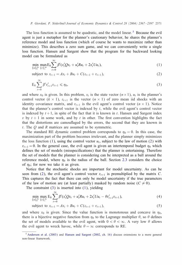
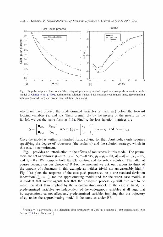
Fig. 1. Impulse response functions of the cost-push process �2t and of output to a cost-push innovation in themodel of Clarida et al. (1999), commitment solution: standard RE solution (continuous line), approximatingsolution (dashed line) and worst case solution (thin dots).

where we have ordered the predetermined variables (e1t and e2t) before the forwardlooking variables (yt and �t). Then, premultiply by the inverse of the matrix on thefar left we get the same form as (11). Finally, the loss function matrices are

Q =

[02×2 02×2

02×2 Qbb

]where Qbb =

[%y 0

0 1

]; R= %i; and U = 04×1:

Once the model is written in standard form, solving for the robust policy only requiresspecifying the degree of robustness (the scalar �) and the solution strategy, which inthis case is commitment.

Fig. 1 provides an introduction to the e;ects of robustness in this model. The param-eters are set as follows: �=0:99, �=0:5, =0:645, !1 =!2 =0:8, #2

1 =#22 =1, %y=0:5,

and %i = 0:2. We compute both the RE solution and the robust solution. The latter ofcourse depends on our choice of �. For the moment we ask our readers to think ofthe amount of robustness in this example as neither trivial nor unreasonably high. 9

Fig. 1(a) plots the response of the cost-push process �2t to a one-standard-deviationinnovation ('2t = 1), for the approximating model and for the worst case model. Itis evident that robust agents fear that the cost-push process �2t will turn out to bemore persistent than implied by the approximating model. In the case at hand, thepredetermined variables are independent of the endogenous variables at all lags; thatis, expectations cannot a;ect any predetermined variable, implying that the trajectoryof �2t under the approximating model is the same as under RE.

9 Formally, � corresponds to a detection error probability of 20% in a sample of 150 observations. (SeeSection 2.3 for a discussion.)


Fig. 1(b) shows the response of output (a forward-looking variable) to the samecost-push shock. The contemporaneous response is the same for the approximatingmodel and for the worst case model, 10 but the dynamic paths are then di;erent,with output feared to be more persistent than suggested by the approximating model.The RE and the approximating solution share the same underlying dynamics for thepredetermined variables, but di;er because of the policy function and of expectationformation.

2.3. Choosing the degree of robustness, �

In formulating a robust control problem, the choice of � is crucial, since the evilagent’s constraint is always binding in a linear-quadratic framework. In other words,the policy function chosen by a robust planner (who prepares for the worst) is tai-lored on a model lying on the boundary of the set from which the evil agent canchoose.

This set is deKned by deviations from the reference model, where the allowed de-viations are decreasing functions of the parameter � (and hence increasing functionsof �0). The choice of the parameter � is therefore crucial, as the planner’s policyfunction will vary with it. Svensson (2002) uses this feature of the solution to stresswhat seems like a weakness of robust control, at least from a Bayesian perspective:a model on the boundary of the available set shapes the policy function, yet modelsoutside this set (including those only an epsilon away) receive no consideration. Healso warns that ‘highly unlikely models can come to dominate the outcome of robustcontrol’ (page 7). In a linear-quadratic framework it is easy to make a robust plannerlook like a foolish catastrophist: her policy function will be implausible if the amountof requested robustness is suNciently large (� is suNciently small).

While these warnings are appropriate, it is usually possible to deKne � so that theplanner looks cautious rather than foolish. As a guide to choosing �, Hansen andSargent adopt a detection error probability approach based on the idea that the modelsin the set should not be easy to distinguish with the available data. Essentially, onetakes an agnostic position on whether the true data generating process is given by theapproximating model or by the worst case model, and chooses a probability of makingthe wrong choice between the two models on the basis of in-sample Kt, for a sampleof given size.

The value of � corresponding to this probability is computed by simulation, invertingthe monotonous function �(�)

�(�) = Probability (LA ¿LW |W )=2 + Probability (LW ¿LA|A)=2; (20)

10 This is a general feature of the Hansen and Sargent solution, and is due to the fact that vt+1 is a functionof variables dated t or earlier.


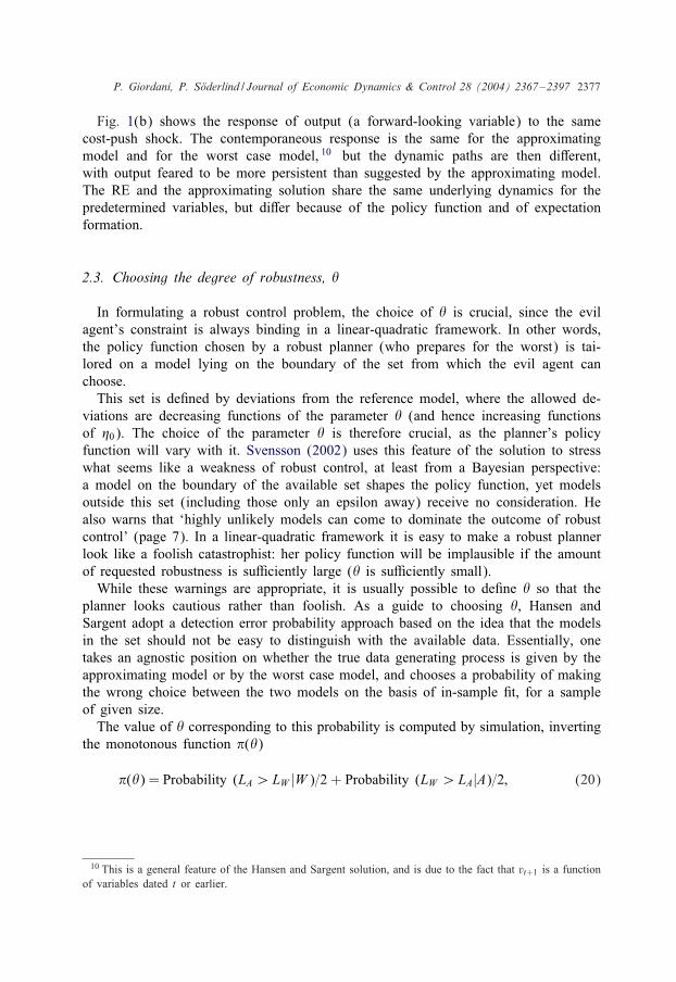
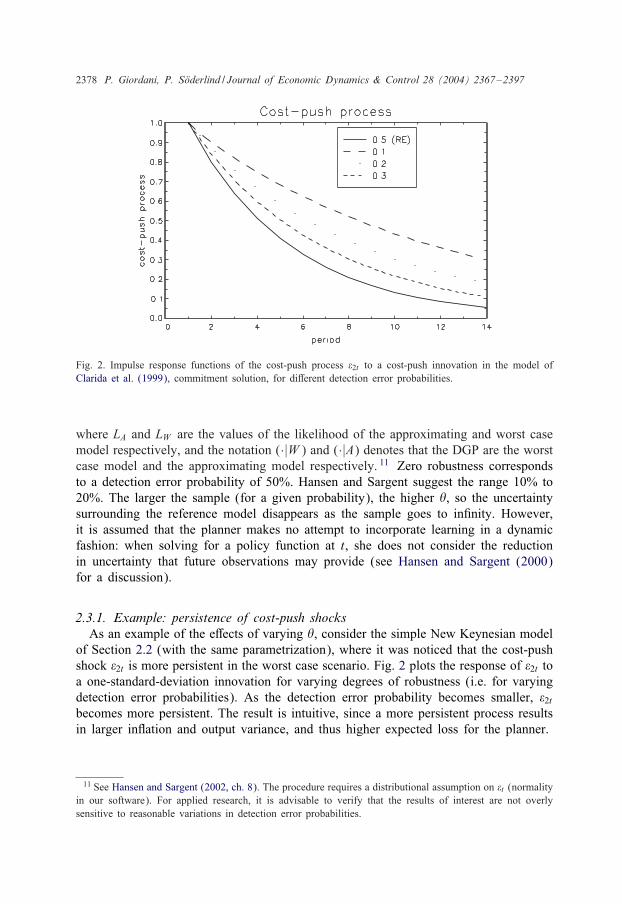
Fig. 2. Impulse response functions of the cost-push process �2t to a cost-push innovation in the model ofClarida et al. (1999), commitment solution, for di;erent detection error probabilities.

where LA and LW are the values of the likelihood of the approximating and worst casemodel respectively, and the notation (·|W ) and (·|A) denotes that the DGP are the worstcase model and the approximating model respectively. 11 Zero robustness correspondsto a detection error probability of 50%. Hansen and Sargent suggest the range 10% to20%. The larger the sample (for a given probability), the higher �, so the uncertaintysurrounding the reference model disappears as the sample goes to inKnity. However,it is assumed that the planner makes no attempt to incorporate learning in a dynamicfashion: when solving for a policy function at t, she does not consider the reductionin uncertainty that future observations may provide (see Hansen and Sargent (2000)for a discussion).

2.3.1. Example: persistence of cost-push shocksAs an example of the e;ects of varying �, consider the simple New Keynesian model

of Section 2.2 (with the same parametrization), where it was noticed that the cost-pushshock �2t is more persistent in the worst case scenario. Fig. 2 plots the response of �2t toa one-standard-deviation innovation for varying degrees of robustness (i.e. for varyingdetection error probabilities). As the detection error probability becomes smaller, �2tbecomes more persistent. The result is intuitive, since a more persistent process resultsin larger in<ation and output variance, and thus higher expected loss for the planner.

11 See Hansen and Sargent (2002, ch. 8). The procedure requires a distributional assumption on �t (normalityin our software). For applied research, it is advisable to verify that the results of interest are not overlysensitive to reasonable variations in detection error probabilities.


3. Robust control with discretion

The discretionary solution coincides with the commitment solution in a backwardlooking model, which has already been treated in Section 2.1.

3.1. Discretion in forward looking models

When working with forward looking models (particularly in the Keld of monetarypolicy) it is often assumed that the planner (the central bank) cannot commit. Sincethis case is of crucial interest, it seems important to extend the robust methods. 12 Inthis section we propose solution concepts and algorithms for dynamic models whichpreserve the property of transforming the problem to a RE form.

In order to illustrate our solution approach to the robust case, it is useful to review themain steps involved in the RE solution (see Backus and DriNl, 1986 or the summaryin Appendix C for a more detailed description of the solution procedure).

1. At time t, the private sector observes x1t and decides on a matrix Kt+1 to usein formulating expectations Ea

t x2t+1 = Kt+1Eat x1t+1, where the notation Ea

t denotesagents’ expectations in period t. The planner moves after the private sector, so thematrix Kt+1 incorporates a guess of the planner’s policy function.

2. At time t, the planner observes x1t and Kt+1 and chooses a policy function ut =−Futx1t+1 to minimize the loss function (1) subject to the law of motion (11) (thesame as in the commitment case), but also subject to the expectation formationprocess Ea

t x2t+1 = Kt+1Eat x1t+1.

3. The equilibrium solution is found when the matrix Kt+1 of the private sector’sexpectations coincides with the mathematical expectation. This happens when thepolicy function Fut implied by Kt+1 is also the policy function that solves theplanner’s problem given Kt+1. In equilibrium Kt+1 and Fut are constant.

Our proposal for dealing with the discretionary case is to extend the principle that,robustness being a metaphor for the planner’s concerns for model misspeciKcation atthe time of choosing a policy function, the evil agent should optimize when and onlywhen the planner does. When applied to the commitment case, this results in Hansenand Sargent’s solution. In the discretionary case, this principle suggests that since theplanner reoptimizes at every period (taking expectations as given), the evil agent shouldbe allowed to do the same. The interpretation is that every time the planner considersa policy, she will have to deal with uncertainty and design a robust rule.

We maintain the assumptions (used by Hansen and Sargent in the commitment case)that the private sector’s loss function, reference model, and � are the same as theplanner’s.

The main steps involved in the RE solution are therefore modiKed as follows to Kndthe robust discretionary policy. First, Kt+1 now implies a guess of the policy functionsof both the planner and the evil agent (private agents share the planner’s concern for

12 Hansen and Sargent (2002, ch. 5) discuss the robust discretionary solution of the static model in Kydlandand Prescott (1977).


robustness). Second, the evil agent chooses a policy function vt+1 = −Fvtx1t (at thesame time as the planner) in order to maximize the loss function, subject to the sameconstraints as the planner, but also subject to the budget Et

∑∞s=1 �svt+svt+s6 �. Third,

in equilibrium both policy rules are constant and consistent with the private sector’sexpectations.

This formulation of the robust discretionary case seems quite natural. Moreover,since � does not depend on t, the size of the deviations from the reference modelcontemplated by the planner is constant through time.

This formulation is also convenient, since it allows us to handle the discretionarycase by augmenting the law of motion and the loss function just like in the commitmentcase. In practice, this means Knding the discretionary solution to the problem detailedin Eqs. (12)–(14). We use algorithms developed for the standard RE discretionary case(see Appendix C), because they solve for the Krst order conditions (which are the samefor the minimum and maximum).

In equilibrium, the predetermined variables (x1t) follow a VAR(1) process

x1t+1 =Mx1t + C1�t+1; (21)

and the forward looking variables and the controls are linear functions of the prede-termined variables

x2t

ut

vt+1

=

N

−Fu

−Fv

x1t : (22)

The only di;erence between the worst case model and the approximating modelis in terms of the M matrix in (21) (see Appendix B for details). The di;erencebetween the two M matrices is therefore a useful indicator of the misspeciKcation thatthe planner fears.

Since (22) is the same, it is clear that the approximating model uses both robustpolicy and robust expectations (the mapping from the predetermined variables to theforward looking variables is very closely tied to expectations).

3.1.1. Application: the simple new Keynesian modelThe model deKned by Eqs. (15)–(19) is written in state space form exactly as for the

commitment solution. Only the solution algorithm changes. The robust policy functiontakes the form given in Eq. (22) and is therefore not history dependent.

Consider the following application. We wish to derive the central bank policy func-tion and the behavior of the economy as the degree of robustness goes from zero (RE)to a � which implies a 20% probability of error detection in a sample of 150 obser-vations. The other parameters are set as in Section 2.2. Fig. 3 shows the results. Eachquadrant plots the response of a variable to a cost push shock ("2t) for three cases:standard RE (�= ∞), the approximating model, and the worst case model.

Robustness leads to higher reactions of all variables at all horizons. The responseof the short interest rate is also higher for the approximating model (when policyis robust but vt+1 is always zero) than for the standard RE case. Finally, the robust


Fig. 3. Impulse response functions of in<ation, output and short interest rate to a cost-push shock in themodel of Clarida et al. (1999), discretionary solution: standard RE solution (continuous line), approximatingsolution (dashed line) and worst case solution (thin dots).

monetary policy function is more aggressive: the policy vector Fu is −(3:0; 1:9)′ for theRE solution, and −(3:5; 2:4)′ for the robust solution. This result is not new, as otherpapers conclude that robustness lead to more aggressive policies under commitment. 13

However, it is of some independent interest that we reach the same conclusion in thediscretionary case.

A recurrent feature of the solution is the evil agent’s common choice of increasing thepersistence of the driving processes. In Fig. 3 the responses of all variables are in factmore persistent in the worst case than in both the standard RE and the approximatingcase. More persistent processes imply higher variances and therefore a greater loss forthe risk averse planner. 14 Fearing this outcome, a robust agent typically has a strongerreaction to shocks than a standard agent. 15

13 See, for instance, Hansen and Sargent (2001), and, with a di;erent approach, Giannoni (2002). However,this result is not general (Hansen and Sargent (2002, ch. 8), provide a counter-example): the outcome willdepend on the model and on the loss function parameters.

14 Hansen and Sargent (2000, 2003) analyze this point at length through spectral analysis, showing howthe evil agent often accentuates the low frequency components of the exogenous processes.

15 Kasa (2001) proves that a robust forecaster, whose loss function is the mean squared error, revises theforecast by more than a standard forecaster following new information, because she is more vulnerable whenshe underestimates the persistence of the driving processes.


This feature of the robust solution, namely the worst case model displaying morepersistence than the approximating model, suggests that we can often expect robustnessto make forward looking prices overreact to news. This implies that robustness makesasset prices more volatile and more forecastable, as illustrated in the applications ofSections 3.1 and 4.1.

3.1.2. Application: the term structure of interest ratesThe literature considered in this paper is young, and yet o;ers several interesting

empirical applications, including consumption/saving decisions (Hansen et al., 1999),asset pricing (Anderson et al., 2003; Hansen et al., 1999; Tornell, 2000; Hansenet al., 2002), and monetary policy rules (Hansen and Sargent, 2001; Giannoni, 2002;Onatski, 2000). In the latter case the focus is on the behavior of the short interestrate (the policy instrument). We suggest a natural extension, namely to consider theimplied behavior of multiperiod interest rates. We continue to work with the model ofSection 2.2. 16 The exercise could be carried out assuming commitment, but discretionis arguably more realistic, so we opt for the latter.

Let it – the policy instrument – be the one period interest rate (not annualized). Weassume that multiperiod rates obey the expectations hypothesis of the term structure.The h-period interest rate (denoted it;h) then follows

it;h = E∗t

h−1∑i=0

it+i ; (23)

where E∗ denotes robust expectations, that is, expectations which condition on the worstcase model. We also deKne a ‘fundamental’ rate, computed substituting the mathemat-ical expectation E for the robust expectation E∗ in Eq. (23). The fundamental ratetherefore guarantees that no expected excess proKts are available, whereas the actualrate does not. Referring to Fig. 3, the actual rate and the fundamental rate are derivedby plugging into Eq. (23) the path of the short interest rate for the worst case modeland for the approximating model respectively.

Fig. 4 shows the di;erence – at the time of a unit shock to the in<ation equation –between a long (h=4) interest rate, and the corresponding fundamental rate, for di;erentdegrees of robustness (represented by error detection probabilities). This di;erence canbe considered an overreaction in the classical sense that the price of the multiperiodbond reacts to a shock by jumping beyond its new equilibrium value (we are assuming,of course, that the approximating model is in fact the DGP). The overreaction is around1.25% at a 20% detection probability, and grows monotonously with the degree ofrobustness.

A rather large empirical literature on the term structure has found that actual changesin short interest rates are smaller than predicted by the slope of the yield curve. 17

Our examples show that robust expectations can contribute to an interpretation of thisKnding.

16 Parameter values are the same as in Section 2.2, and � again implies a detection error probability of20% in a sample of 150 observations.

17 See, for example, Walsh (1998, ch. 10) and Campbell et al. (1997, ch. 10).


Fig. 4. Over-reaction of the long interest rate to a CP shock as a function of the degree of robustness (interms of the detection error probability) in the model of Clarida et al. (1999) with discretionary solution.0.01 corresponds to one basis point.

3.1.3. Application: the in@ation biasA well known example of how the presence or absence of a commitment technology

can a;ect an economic outcome is the time inconsistency of optimal monetary policyKrst studied by Kydland and Prescott (1977) and Barro and Gordon (1983). Theyassume that the planner is targeting a level of output above potential output, andthen show that the discretionary solution involves an in<ation bias (in<ation is higherthan the optimal level). The model of Kydland and Prescott is static and involvesexpectations about the control variable, so it cannot be cast into the form of Eq. (11).However, an analytical solution is available. Hansen and Sargent (2002) show that fearof misspeciKcation increases the in<ation bias. The intuition is that the planner fearsthat the expected value of output is lower than in the reference model, which increasesthe distance between desired and expected output. Thus a preference for robustness hasthe same e;ect as an increase in target output: higher in<ation.

With our solution approach for discretion in dynamic models, we can recast Hansenand Sargent’s exercise in more general settings. Here we study the in<ation bias in thedynamic model of Clarida et al. (1999) used in the previous section (Eqs. (15)–(19)),except that we allow for an output target level y∗ ¿ 0 in the loss function, whichbecomes

Et

∞∑s=0

�s[�2t+s + %y(yt+s − y∗)2 + %ii2t+s]: (24)

Technically, this requires adding the constant 1 to the vector of predetermined vari-ables. Average in<ation in the standard RE solution is then a positive function of y∗.In our proposed solution for the discretionary case, the evil agent’s control vector, vt+1,


Fig. 5. In<ation bias as a function of the detection error probability in the model of Clarida et al. (1999).The horizontal line gives the in<ation bias for the RE solution.

is a linear function of the predetermined variables, just like the central bank’s policyrule.

It turns out that the evil agent decides to a;ect both the constant and the autore-gressive parameters, thus increasing both the mean of in<ation and its variance. Theconstant is negative because y∗ is positive. Intuitively, since the loss function is sym-metric in y around y∗ while the evil agent’s cost is symmetric in y around zero, it ischeap and e;ective for the evil agent to set a negative constant to output. The result isthat robustness leads to an increase of average in<ation in the discretionary solution,for the same reason as in the Kydland-Prescott example.

Fig. 5 shows how the in<ation bias varies with the degree of robustness in themodel of Clarida et al. (1999). The calibration is the same as in Section 2.2. We sety∗ to 0.4. The in<ation rate is deKned as the growth rate in prices during one period.Therefore, if we think of the model as applying to quarterly data, an in<ation bias of0:8% translates into an annual bias of approximately 3:2%.

4. Robust control with simple rules

The monetary policy literature has paid a good deal of attention to the propertiesof simple rules, deKned as commitment rules that set the policy instrument as a linearfunction of the system variables. Examples include Taylor type rules and rules formoney growth. Simple rules are typically not optimal. In some cases they are motivatedas good empirical approximations to actual policy.

In other cases simple rules are justiKed as an attempt to identify rules that workwell in a variety of models. A prominent proponent of robustness in this sense isMcCallum (1988, 1999). An interesting example is Levin et al. (2001), who focus on


simple monetary policy rules that work well in models that incorporate rather di;erentviews of the transmission mechanism. 18

This literature uses the term robust for a rule that performs well across models.Hansen and Sargent propose, instead, to design rules that perform well for deviationsaround a single model. Sims (2001a) argues that a Hansen–Sargent robust solution to asingle reference model may in fact not be robust in the sense of McCallum. There is ofcourse no reason why the two concepts should be substitutes rather than complements:one could try to identify a rule that is robust in a Hansen–Sargent’s sense for severalreference models, or, when possible, merge the competing models and thus reducemodel uncertainty to parameter uncertainty. A preliminary requirement for this is tospecify solution concepts for simple rules in a Hansen–Sargent robust framework. Asolution for backward looking models is already available, and one for forward lookingmodels is proposed in this section.

Another reason why we are interested in simple rules in a robust framework is thatthey allow us to isolate the e;ects of the private sector deviations from RE. In e;ect,a planner who has committed to a given simple rule is no longer involved in anydecision, so any change in economic outcome between the RE and the robust solutionis entirely due to the role of private sector expectations.

4.1. Simple rules in backward looking models

Managing a simple rule in a backward looking model is a straightforward applicationof the robust pure prediction problem analyzed in Hansen and Sargent (2002) andKasa (2001). The planner commits to a speciKc Fu in setting ut =−Fuxt (where xt canbe augmented by any variables that are important for policy decisions). Then the evilagent is left with the following program

max{v}∞

1

E0

∞∑t=0



t+1vt+1)

subject to xt+1 = (A − BFu)xt + C(vt+1 + �t+1); (25)

and where x0 is given. This is a standard RE problem of Knding the optimal policyrule in a backward looking model. The evil agent will therefore choose to set vt+1 asa linear function of the state xt .

Example (A simple forecasting problem): As an illustration, consider a simple robustforecasting problem. Let the loss function be the mean squared forecast error Et(xt+i −xet+i; t)

2, where xet+i; t denotes the forecast of xt+i made at time t. Suppose that xt is theamount of dividends. The reference model of the dividend is an AR(1) process (A in(25) is the autoregressive coeNcient and B= 0).

It is straightforward to show that the robust forecast of xt+i at time t, denoted byE∗t xt+i, is E∗

t xt+i = (A∗)ixt ; where A∗ ¿A so the investor forecasts as if the processdriving dividends was more persistent than in the reference model. The investor thus

18 Leitemo and S/oderstr/om (2004) evaluate the performance of simple monetary policy rules (compared tooptimal rules) in several variations of a baseline model.


fears that the process has high persistence. The intuition is that more persistence giveslarger uncertainty of long horizon forecasts (as future shocks are propagated more).

If the asset price is the discounted (at rate �) sum of expected dividends, then weget the price xt=(1−A∗�). Since A∗ is a positive function of the degree of robustness,so too is the price variance. 19 A small degree of robustness can have large e;ectson the behavior of prices. For example, let � = 0:98, and A = 0:99, and A∗ = 1. Thisrelatively small degree of robustness implies an increase of around 50% in the standarddeviation of the asset price.

4.2. Simple rules in forward looking models

The forward looking case is less straightforward. We propose to be more speciKcabout the set of models from which the evil agent can choose (that is, the type ofmisspeciKcation feared), by imposing that he sets his instruments vt+1 as a linearfunction of predetermined variables. That is, we allow for misspeciKcations of theform

vt+1 = −Fvx1t ; (26)

and leave the evil agent free to choose the coeNcients of the (n1 × n1) matrix Fv

(within the limits of the budget deKned by �).For the moment we concentrate on the technical aspects of our proposed solution,

postponing its motivation to the end of this section. Formally, we suggest to set upthe problem as

maxFv

E0

∞∑t=0



t+1vt+1);

subject to (11); (26) and ut = −Fuxt ; (27)

and where x10 is given. The constraint vt+1 = Fvx1t has been imposed and the maxi-mization is explicitly in terms of Fv. The interpretation is that the planner is fearingerrors in the coeNcients which relate predetermined variables to lags of predeterminedvariables. As in previous cases, the problem can be written as a standard RE problem

maxFv

E0

∞∑t=0


t′R∗u∗

t + 2x′tU

∗u∗t );

subject to (13) and u∗t =

[ −Fu

−Fv 0n1×n2

]xt ; (28)

where x10 is given and the starred (∗) matrices are deKned in (14).For given Fu and Fv, the solution concept is that of a simple rule in a forward

looking model: private sector expectations are consistent with the evolution of theeconomy in the worst case model. The solution to (28) is then found by letting a

19 See Hansen and Sargent (2002), from which this example is adapted.


numerical maximization routine search over Fv (the policy rule Fu is kept constant).The solution algorithm is outlined in Appendix C.

The formal representation of the equilibrium can be written in the same form asin the discretionary case (21)–(22) where the predetermined variables (x1t) followa VAR(1) process and the other variables are linear functions of the predeterminedvariables (see Appendix B for details).

Example (The simple new Keynesian model): The state space form is as for thecommitment and discretionary solution, except that the researcher must provide a matrixFu (and of course a value of �).

4.2.1. Motivation of our robust simple solutionWe will now motivate our proposed solution for the simple rule in a forward looking

model. Recall that we are constraining the vt+1 to be a linear function of predeterminedvariables. Why this constraint? The problem is that an evil agent free to commit toany rule uses agents’ expectations to his advantage, and therefore makes the set ofplausible models dependent on the expectation formation. By strategically exploitingexpectations, an agent free to commit can drive the loss function to inKnity for anydegree of robustness, for example by committing to an exponentially increasing ordecreasing series of vt+1, a highly improbable misspeciKcation to fear. This does nothappen when the planner is allowed to choose a robust policy (in the commitment ordiscretionary case) – but it happens with a simple rule since the policy maker is boundto follow a given rule. To put it simply, the planner is defenceless against the evilagent.

On the other hand, the choice of constraining vt+1 to be linear in the predeterminedvariables ensures that the set of misspeciKcations that the planner considers plausibleis given exogenously, in the sense that it does not depend on how expectations areformed, and that there is a Knite � for which a model that has stable dynamics underRE remains stable in the robust solution.

The following example illustrates the argument. Let the planner’s loss function de-pend on squared in<ation rates, L0 = E0

∑∞t=0 �t�2

t , and the law of motion of theeconomy be given by the simpliKed Calvo style Phillips curve

�t = �Et�t+1 + �t ; where �t is iid with E�t = 0 and Var(�t) = 1:

In this case, the planner has no e;ect at all on in<ation – but the more general pointis that she cannot revise her policy to defend against the evil agent. Assume that theevil agent can commit to any policy rule. He therefore solves 20

max{v}∞

1

E0

∞∑t=0

�t�2t

subject to �t = �Et�t+1 + vt+1 + �t and E0

∞∑t=0

�tv2t+16 �0: (29)

20 We write the evil agent’s constraint explicitly rather than in terms of the Lagrange multiplier �: A high�0 corresponds to a low �. We also set c = std(�t) = 1.


It is straightforward to prove that an evil agent who is able to commit will choose anon-stationary (exponentially increasing or decreasing) vt+1 (see Appendix D), whichmakes the loss function unbounded for any strictly positive �0. The misspeciKcationfeared is then a trend increase (or decrease) of in<ation, which is a case of limitedinterest.

In contrast, this problem has a well deKned solution under our proposed approachto the simple rule case, which here forces the evil agent to set vt+1 as a function of �t(the only predetermined variable), say vt+1 = a�t . The robust expectations are thereforeformed as if the standard deviation of the errors was 1 + a rather than 1.

4.2.2. Application: output and in@ation volatilityThe di;erences between the robust and RE solutions illustrated in Fig. 3 are due to

deviations from rational expectations of both the planner and the private sector. Thesolution approach to simple rules in forward looking models developed in Section 4.2opens up the possibility of isolating the e;ects of private sector deviations from RE.We might then ask how a preference for robustness on the part of the private sectora;ects macroeconomic variables and asset prices, keeping the behavior of the plannerKxed by assuming that she has committed to a simple rule.

To illustrate, we continue to consider the simple model of Section 2.2. The goal isto establish a link between the degree of robustness and the volatility of in<ation andoutput.

The central bank is assumed to commit to the Taylor rule

it = 1:5�t + 0:5yt:

The solution takes the form[x2t

vt+1

]=

[N

−Fv

]x1t : (30)

As in the other equilibria, N is a function of � and does not depend on whether theplanner’s fears are founded or not (that is, the approximating model and the worst casemodel share the same way of forming expectations).

We assume that the approximating model is correct, and therefore that x1t evolvesas (see Appendix B)

x1t+1 =Max1t + C1�1t ; (31)

from which we obtain the variance of the predetermined shocks (e1t and e2t). Thematrix N in (30) is then used to compute the variance of the corresponding series ofoutput and in<ation. This is done for the standard RE case (�=∞) and for the robustcase.

The variance of output and in<ation is found to be a monotonous function of thedegree of robustness (an inverse function of �). At �=850, which corresponds to a 20%error detection probability for a sample of 150 observations, the variances of outputand in<ation are some 3% and 46% higher than in the standard RE case respectively.

To gain some intuition for this result, it is useful to compare the matrix Ma, whichactually generates the predetermined variables in (31), and M , which corresponds to


the worst case model and therefore to agents’ expectations (see Appendix B). Theparameters in Ma are !1 and !2

Ma =

[0:8 0

0 0:8

];

while M (the worst case model) is

M =

[0:86 0:04

0:02 0:82

]:

Comparing Ma and M , we notice that the private sector is fearing that the exogenousprocesses are more persistent than in the approximating model. Expecting persistentdynamics of the driving processes (the predetermined variables), consumers and pricesetters overreact to news, in the sense that output and in<ation have a stronger responseto shocks than in the RE case.

Using the same model we can isolate the e;ects of robust expectations on the termstructure. The results (not reported) are similar to those of the discretionary solution,shown in Figs. 3 and 4: the public fears more persistent e;ects of shocks and multi-period interest rates overreact. 21

4.2.3. Application: publishing central bank forecastsSims (2001a) argues that a min–max approach to robustness is better suited to cap-

ture agents’ near rational behavior than as a normative course of action for centralbanks. The following example embraces his point of view and departs from the as-sumption that the private sector and the central bank share the same information andthe same taste for robustness. We assume that the central bank has a good and preciselyestimated model, while the private sector nurtures strong doubts about the behavior ofthe economy.

To simplify the problem as much as possible, we make the following assumptions.First, the private sector does not know the model (or simply the coeNcients) estimatedby the central bank, but it knows that the bank has an accurate representation of theeconomy. Second, the central bank follows the Taylor rule it = 1:5�t + 0:5yt . Third,the private sector’s reference model is the same as the central bank’s and it is also theDGP.

The second assumption means that we can adopt the simple rule solution developedin Section 4.2. Altogether, these three assumptions are admittedly unrealistic, but theyhelp us make the following point: the central bank can reduce the variance of in<ationand output by releasing information to the public, for example in the form of forecasts.To verify the statement, notice that if the central bank does not release information, thesetup and outcome is exactly as in the previous application, where robustness increasesbusiness cycle volatility. However, if the central bank announces its forecasts of thepredetermined variables, the private sector makes these forecasts their own (by the Krstassumption), taking the economy back to the superior RE solution.

21 We obtained similar results on the behavior of long interest rates in the model of Fuhrer (1997), withthe parameters estimated in S/oderlind (1999).


Whether central banks should release explicit forecasts is a matter of current debate(see Svensson (2001) for a list of central banks that do, and arguments in favor of thepractice). While our example cannot be a serious attack on the issue, it does lead usto believe that a more thorough investigation would be worth the e;ort.

5. Conclusions

The approach to dealing with model uncertainty proposed by Lars Hansen andThomas Sargent seems promising from both a normative (designing a rule that workswell in a neighborhood of the reference model) and a descriptive (replicating the be-havior of actual agents) perspective. In the discussion of Kscal and monetary policy,much of the debate is centered around two non-history dependent sets of policies: sim-ple rules and discretionary solutions, which Hansen and Sargent do not consider. Thispaper proposes solution approaches for simple rules and discretion. These extensionspreserve the property that the robust program can be written and solved as a suitablymodiKed rational expectations program. Some applications show that these extensionscan be interesting for applied work. The analysis of the term structure of interest ratescomplements previous research and suggests that standard models give a better em-pirical description of asset returns if agents are attributed a taste for robustness. Theresult that the in<ation bias increases with robustness can be interpreted as saying thatthe gains from commitment increase if potential output is imprecisely estimated. Theapplication to the variance of in<ation and output for a given policy function is per-haps the most interesting. It suggests that a robust private sector may amplify thosesame <uctuations in in<ation and output that it fears, and can provide a theoreticalmotivation for central banks to be transparent about their forecasts.

Acknowledgements

The authors thank Adrian Pagan, Wouter Den Haan, Noah Williams, an anonymousreferee, and seminar participants at the Swedish Central Bank and at the University ofNew South Wales for comments.

Appendix A. Software

Our software can be downloaded freely at http://home.tiscalinet.ch/paulsoderlind. Auser’s manual and example programs are provided. The procedures follow the notationof this paper, and their syntax is therefore immediately understood. The user needs towrite the loss function (that is, specify �; Q; R; U ), write the model in state space form(that is, specify A; B; C; n1), select a �, and decide on a solution algorithm (commitment,discretion, simple rule). Advanced users can Kne tune the optimization algorithms.Bayesian error detection probability is also implemented (assuming normally distributederrors) to assist the user in selecting �. We follow Hansen and Sargent in plotting the

http://home.tiscalinet.ch/paulsoderlind


probability (of selecting the wrong model) against #=−1=�, rather than against �. ToKnd the � corresponding to a probability of 0.2 in the Euler+Calvo model (discretionarysolution), we solved the model 10,000 times. This took around 20 s on a Pentium IIIPC using Gauss, and a few seconds more using Matlab.

Appendix B. Reduced form dynamics of the forward looking models

This appendix shows how to compute the dynamics of the worst case and of theapproximating model for the forward looking commitment case. The dynamics of theforward looking discretionary and simple rule cases have the same general form, butwith !2t being an empty vector (or a vector of zeros).

The solution can be written in the following general form (see Appendix C)[x1t+1

!2t+1

]=M

[x1t

!2t

]+ C�t+1; (B.1)

x2t

ut

vt+1

!1t

= N

[x1t

!2t

]=

N1

N2

N3

N4

[x1t

!2t

]; (B.2)

with !20 = 0n2×1. In the discretionary and simple rule solutions, !2t = 0 for all t.Eqs. (B.1) and (B.2) give the dynamics of the worst case model. To retrieve the dy-namics of the approximating model, we rewrite (B.1) as[

x1t+1

!2t+1

]=M

[x1t

!2t

]+ C�t+1; (B.3)

where

M = P−1(A − BFu − BFv)P

P =

[In1 0n1×n2

N1

]⇒

[x1t

x2t

]= P

[x1t

!2t

]; and

[ut

vt+1

]=

[N2

N3

]P−1

[x1t

x2t

]=

[ −Fu

−Fv

] [x1t

x2t

]: (B.4)

We then set Fv = 0n1×n in (B.3), so[x1t+1

!2t+1

]=Ma

[x1t

!2t

]+ C�t+1; (B.5)

where Ma = P−1(A− BFu)P. The values x1t and x2t are then determined by (B.5) and(B.2). In applications, Ma is sometimes not a function of �. This happens when thepredetermined variables are block exogenous, that is, independent of lagged values ofthe forward looking variables.


Appendix C. Solution algorithms

This appendix summarizes the solution algorithms by adapting some material inS/oderlind (1999). The forward looking models are in the main focus, but we alsocomment on how backward looking models can be handled.

C.1. Optimal policy under commitment

The Lagrangian of the forward looking model (12)–(13) is

L0 = E0

∞∑t=0

�t[x′tQxt + 2x′

tU∗u∗

t + u∗t′R∗u∗

t

+2!′t+1(Axt + B∗u∗

t + "t+1 − xt+1)]; (C.1)

where "t+1 = (C�t+1; x2t+1 − Etx2t+1). Let n= n1 + n2 be the number of elements in xtand let q= k + n1 be the number of elements in u∗

t .The Krst order conditions with respect to !t+1, xt , and u∗

t are

In 0n×q 0n×n

0n×n 0n×q �A′

0q×n 0q×q −B∗′

xt+1

u∗t+1

Et!t+1

=

A B∗ 0n×n

−�Q −�U ∗ In

U ∗′ R∗ 0q×n

xt

u∗t

!t

+

"t+1

0n×1

0q×1

: (C.2)

Take conditional expectations of (C.2), expand xt and !t as (x1t ; x2t) and (!1t ; !2t)respectively, and reorder the rows by placing !2t after x1t . Write the result as

GEt

[kt+1

%t+1

]= D

[kt

%t

]; where kt =

[x1t

!2t

]and %t =

x2t

u∗t

!1t

: (C.3)

The elements in kt have initial conditions: the initial state vector x10 is given and theforward looking variables can be chosen freely in the initial period so their shadowprices !20 are zero (see Currie and Levine, 1993).

Given the square matrices G and D in (C.3), the generalized Schur decompositiongives the square complex matrices Q (not the same Q as in (C.1)), S, T , and Z suchthat G = QSZH and D= QTZH , where ZH denotes the transpose of the complex con-jugate of Z . Q and Z are unitary (QHQ= ZHZ = I), and S and T are upper triangular– see Golub and van Loan (1989). Reorder the decomposition (see Sims, 2001b andKlein, 2000) so the block corresponding to the stable (modulus less than one) gen-eralized eigenvalues (the diagonal of T divided by the corresponding elements in S)come Krst.


Introduce the auxiliary variables[�t

7t

]= ZH

[kt

%t

]; (C.4)

where �t corresponds to the stable eigenvalues.Use the generalized Schur decomposition in (C.3), premultiply by QH , use the def-

initions in (C.4), and partition S and T conformably with �t and 7t to get[S�� S�7

0 S77

]Et

[�t+1

7t+1

]=

[T�� T�7

0 T77

] [�t

7t

]: (C.5)

Since the lower right block contains the unstable roots, 7t will diverge unless 70 = 0.From (C.5) we see that any stable solution will therefore have 7t = 0 and

Et�t+1 = S−1�� T��t ; (C.6)

since S�� is invertible (follows from the way we have ordered the eigenvalues).From (13) x1t+1 −Etx1t+1 =C1�t+1 and Backus and DriNl (1986) show that !2t+1 −

Et!2t+1=0. Using (C.3), stack these expressions as kt+1−Etkt+1. Invert (C.4), partitionconformably with kt , %t , �t and 7t , and use the fact that 7t = 0[

kt

%t

]=

[Zk� Zk7

Z%� Z%7

] [�t

7t

]=

[Zk�

Z%�

]�t : (C.7)

It follows that kt+1 − Etkt+1 can be written

Zk�(�t+1 − Et�t+1) =

[C�t+1

0

]: (C.8)

We can solve for �t+1 in (C.8) if Zk� is invertible. A necessary condition is that thenumber of backward looking variables (the number of rows in Zk�) equals the numberof stable roots (the number of columns in Zk�) – this is the saddlepoint condition inproposition 1 of Blanchard and Kahn (1980). Assuming this is satisKed, solve for �t+1

and substitute for Et�t+1 from (C.6)

�t+1 = S−1�� T��t + Z−1

k�

[C�t+1

0

]: (C.9)

The last step is to combine this expression with (C.7) and the deKnitions in (C.4) towrite the dynamics as[

x1t+1

!2t+1

]=M

[x1t

!2t

]+

[C�t+1

0

]; where M = Zk�S

−1�� T��Z

−1k� ; (C.10)

x2t

u∗t

!1t

= N

[x1t

!2t

]; where N = Z%�Z

−1k� ; (C.11)

and where x10 is given and !20 = 0.


This algorithm can also be used for the backward looking case (although there aresimpler algorithms that also work): x2t and !2t+1 are then empty vectors and n= n1.

C.2. Optimal policy under discretion

This section summarizes the iterative algorithm for the discretionary case used byBackus and DriNl (1986). The policy maker reoptimizes every period by taking theprocess by which private agents form their expectations as given. The solution in t+1gives a value function which is quadratic in the state variables, x′

1t+1Vt+1x1t+1 + vt+1,and a linear relation between the forward looking variables and the state variables,x2t+1 = Kt+1x1t+1. Private agents form expectations about x2t+1 accordingly.

Partition the matrices A; B∗; Q; U ∗, and C in (12)–(13) conformably with x1t and x2t .The Bellman equation for the optimization problem can then be written

x′1tVtx1t + wt =minmax

u∗t

[x′1t Qtx1t + 2x′

1t U tu∗t + u∗

t′Rtu∗

t

+ �Et(x′1t+1Vt+1x1t+1 + wt+1)]

s:t: x1t+1 = Atx1t + Btu∗t + C1�t+1 and x1t given; (C.12)

where the matrices with a tilde (∼) are deKned as

Dt = (A22 − Kt+1A12)−1(Kt+1A11 − A21)

Gt = (A22 − Kt+1A12)−1(Kt+1B∗1 − B∗

2 )

At = A11 + A12Dt

Bt = B1 + A12Gt

Qt = Q11 + Q12Dt + D′tQ21 + D′

tQ22Dt

U t = Q12Gt + D′tQ22Gt + U ∗

1 + D′tU

∗2

Rt = R∗ + G′tQ22Gt + G′

tU∗2 + U ∗

2′Gt: (C.13)

The Krst order conditions of (C.12) with respect to u∗t are

u∗t = −F1tx1t ; F1t = (Rt + �B′

tVt+1Bt)−1(U ′t + �B′

tVt+1At): (C.14)

Combining with (C.12) gives

x2t = Ktx1t ; with Kt = Dt − GtF1t ; and (C.15)

Vt = Qt − U tF1t − F ′1t U

′t + F ′

1t RtF1t + �(At − BtF1t)′Vt+1(At − BtF1t): (C.16)

The algorithm involves iterating until convergence (‘backwards in time’) on (C.13)–(C.16). It should be started with a symmetric positive deKnite Vt+1 and some Kt+1. IfF1t and Kt converge to constants F1 and K , the dynamics of the model are (rewrite


the Krst n1 equations of (13))

x1t+1 =Mx1t + C�t+1; where M = A11 + A12K − B∗1F1; (C.17)[

x2t

u∗t

]= Nx1t ; where N =

[K

−F1

]: (C.18)

For a backward looking model, the discretionary solution coincides with the com-mitment solution (see above for a solution algorithm).

C.3. An optimal simple rule

We start by Knding the equilibrium for a given ‘decision rule’ of the evil agent,Fv, and the private sector, Fu. Use the expression for u∗

t in (28) in (13) and takeconditional expectations to get

Et

[x1t+1

x2t+1

]= D

[x1t

x2t

]; where D = A+ B∗

[ −Fu

−Fv 0n1×n2

]: (C.19)

This has the same form as (C.3), so the same solution method can be used: the solution(C.10)–(C.11) still applies. The only di;erence is that u∗

t , !1t+1, and !2t+1 are emptyvectors here.

It is straightforward to show that the loss function value for given Fu and Fv matricesis

J0 = x′10Vx10 + trace(VC1C′

1)�=(1 − �); (C.20)

where the matrix V is the Kxed point in the iteration (‘backwards in time’) on

Vs = P′[

Q U ∗

U ∗′ R∗

]P + �M ′Vs+1M; where P =

In

−Fu

−Fv

[In1

N

]; (C.21)

where M and N are from the solution (C.10)–(C.11). The evil agent maximizes theloss function (C.20) by choosing the optimal elements in the decision rule Fv. Thisrule is found by a non-linear optimization algorithm.

For a backward looking model, the solution is trivial, but the algorithm here canstill be used if we set x2t to an empty matrix.

Appendix D. The stability problem of robust simple rules

Proposition 1. If �0 is strictly positive, the loss function is unbounded. This outcomecan be achieved by the evil agent committing to an ever increasing (or decreasing)constant in the law of motion.

Proof. Assume that the evil agent commits to the sequence vt+1 = �t , ¿ 0. Then

E0�t =∞∑s=0

�svt = �t

1 − ��: (D.1)


The constraint is binding, so �0 = 2(1 − ��2) and the problem can be written as

max�

2

(1 − ��2)(1 − ��)2; s:t: 1 − ��2 ¿ 0: (D.2)

This problem does not have a maximum: �=√

1=� is a supremum. However, the evilagent can pick a �∗ such that 1¡�∗ ¡

√1=�, which in turn makes the loss unbounded

by (D.2), and limt→∞ E0�t = ∞ by (D.1).

References

Anderson, E., Hansen, L.P., Sargent, T.J., 2003. Robustness, detection, and the price of risk. StanfordUniversity Working Paper.

Backus, D., DriNl, J., 1986. The consistency of optimal policy in stochastic rational expectations models.CEPR Discussion Paper 124.

Barro, R.J., Gordon, D.B., 1983. Rules, discretion, and reputation in a model of monetary policy. Journal ofMonetary Economics 12, 101–121.

Blanchard, O.J., Kahn, C.M., 1980. The solution to linear di;erence models under rational expectations.Econometrica 5, 1305–1311.

Brainard, W., 1967. Uncertainty and the e;ectiveness of policy. American Economic Review 57, 411–425.Campbell, J.Y., Lo, A.W., MacKinlay, A.C., 1997. The Econometrics of Financial Markets. Princeton

University Press, Princeton, NJ.Clarida, R., GalWX, J., Gertler, M., 1999. The science of monetary policy: a new Keynesian perspective. Journal

of Economic Literature 37, 1661–1707.Currie, D., Levine, P., 1993. Rules, Reputation and Macroeconomic Policy Coordination. Cambridge

University Press, Cambridge.Epstein, L.G., Melino, A., 1995. A revealed preference analysis of asset pricing under recursive utility.

Review of Economic Studies 62, 597–618.Epstein, L.G., Schneider, M., 2003. Recursive multiple-priors. Journal of Economic Theory 113, 1–31.Epstein, L.G., Wang, T., 1994. Intertemporal asset pricing under knightian uncertainty. Econometrica 62,

283–322.Fuhrer, J.C., 1997. In<ation/output variance trade-o;s and optimal monetary policy. Journal of Money, Credit,

and Banking 29, 214–234.Giannoni, M.P., 2002. Does model uncertainty justify caution? robust optimal monetary policy in a

forward-looking model. Macroeconomic Dynamics 6, 111–144.Gilboa, I., Schmeidler, D., 1989. Maxmim expected utility with non-unique prior. Journal of Mathematical

Economics 18, 141–153.Golub, G.H., van Loan, C.F., 1989. Matrix Computations, 2nd Ed. The John Hopkins University Press,

Baltimore, MD.Hansen, L.P., Sargent, T.J., 2000. Wanting robustness in macroeconomics. Stanford University Working

Paper.Hansen, L.P., Sargent, T.J., 2001. Acknowledging misspeciKcation in macroeconomic theory. Review of

Economic Dynamics 4, 519–535.Hansen, L.P., Sargent, T.J., 2002. Robust control and model uncertainty in macroeconomics. Stanford

University manuscript.Hansen, L.P., Sargent, T.J., 2003. Robust control of forward-looking models. Journal of Monetary Economics

50, 581–604.Hansen, L.P., Sargent, T.J., Tallarini, T., 1999. Robust permanent income and pricing. Review of Economic

Studies 66, 873–907.Hansen, L.P., Sargent, T.J., Wang, N.E., 2002. Robust permanent income and pricing with Kltering.

Macroeconomic Dynamics 6, 40–84.Kasa, K., 2001. A robust Hansen–Sargent prediction formula. Economic Letters 71, 43–48.


Klein, P., 2000. Using the generalized schur form to solve a multivariate linear rational expectations model.Journal of Economic Dynamics and Control 24, 1405–1423.

Knight, F., 1921. Risk, uncertainty and proKt. London School of Economics, London.Kydland, F.E., Prescott, E.C., 1977. Rules rather than discretion: the inconsistency of optimal plans. Journal

of Political Economy 85, 473–491.Leitemo, K., S/oderstr/om, U., 2004. Simple monetary policy rules and exchange rate uncertainty. Journal of

International Money and Finance, forthcoming.Levin, A., Wieland, W., Williams, J.C., 2001. The performance of forecast-based monetary policy rules

under model uncertainty. Finance and Economics Discussion Series 39 Board of Governors of the FederalReserve System.

McCallum, B.T., 1988. Robustness properties of a rule for monetary policy. Carnegie-Rochester ConferenceSeries on Public Policy 29, 173–203.

McCallum, B.T., 1999. Issues in the design of monetary policy rules. In: Taylor, J.B., Woodford, M. (Eds.),Handbook of Macroeconomics. Elsevier, Amsterdam.

Onatski, A., 2000. Robust monetary policy under model uncertainty: incorporating rational expectations.Harvard University Working Paper.

Onatski, A., Williams, N., 2003. Modeling model uncertainty. Princeton University Working Paper.Sims, C.A., 2001a. Pitfalls of a minimax approach to model uncertainty. Princeton University Discussion

Paper.Sims, C.A., 2001b. Solving linear rational expectations models. Journal of Computational Economics 20,

1–20.S/oderlind, P., 1999. Solution and estimation of RE macromodels with optimal policy. European Economic

Review 43, 813–823.Svensson, L.E.O., 2001. What is good and what is bad with the eurosystem’s published forecasts, and how

can they be improved?. Princeton University manuscript.Svensson, L.E.O., 2002. Robust control made simple. Princeton University manuscript.Tornell, A., 2000. Robust-h∞ forecasting and asset pricing anomalies. NBER Working Paper No. 7753.Walsh, C.E., 1998. Monetary Theory and Policy. MIT Press, Cambridge, MA.

Documents

Solution of macromodels with Hansen–Sargent robust ...kkasa/soderlin.pdf · ... the time inconsistency of optimal monetary policy, ... equilibrium; robustness in ... two-agent representation: