Embed Size (px)
Citation preview
ii
“APPENDIX-D˙WEB” — 2012/3/2 — 18:51 — page 1 — #1 ii
ii
ii
1
Solution of Linear AlgebraicEquations by Gauss Elimination
Simultaneous linear algebraic equations arise in methods for analyzing many differentproblems in solid mechanics, and indeed other branches of engineering science. Inthis book alone, we meet examples in the analysis of both statically determinate andstatically indeterminate pin-jointed structures, the finite element analysis of beams,the analysis of strain gage measurements, and the determination of stresses in thick-walled cylinders. Gauss elimination is a direct method for solving such equations bysuccessive elimination of the unknowns. Let us consider first an example involvingjust three equations
2x1 + x2 − x3 = 1
x1 + 3x2 + 2x3 = 13 (1)
x1 − x2 + 4x3 = 11
where x1, x2, and x3 are the unknowns to be found. We can use the first equation toeliminate x1 from the other two equations. To do this, we divide the first equationthrough by 2 and subtract from the second and third equations to give
2x1 + x2 − x3 = 1
2.5x2 + 2.5x3 = 12.5 (2)
−1.5x2 + 4.5x3 = 10.5
Similarly, the second of these is multiplied through by 1.5/2.5 and added to the thirdequation to eliminate x2
2x1 + x2 − x3 = 1
2.5x2 + 2.5x3 = 12.5 (3)
6x3 = 18
Solving these equations in reverse order, a process known as back substitution, weobtain: x3 = 3, then x2 = (12.5−2.5×3)/2.5 = 2, and finally x1 = (1−2+3)/2 = 1.
ii
“APPENDIX-D˙WEB” — 2012/3/2 — 18:51 — page 2 — #2 ii
ii
ii
2 SOLUTION OF LINEAR EQUATIONS
Let us now try to generalize this process to any set of n linear equations, whichwe may express in the general form
a11x1 + a12x2 + . . . + a1nxn = b1
a21x1 + a22x2 + . . . + a2nxn = b2
. . . . . . . . . . . . . . . . . . . . . . . . . . . . . . . . . (4)
an1x1 + an2x2 + . . . + annxn = bn
where the coefficients aij and bi are all known constants. We may also write theseequations in matrix form as
a11 a12 . . . a1na21 a22 . . . a2n. . . . . . . . . . . .an1 an2 . . . ann
x1x2...xn
=
b1b2...bn
(5)
orAX = B (6)
where A is an n×n square matrix, and X and B are column vectors or n×1 matrices.We may represent the general coefficients in these matrices as aij , xi, and bi, wheresubscript i specifies the row number, and j defines the column number.
In order to define the elimination process, let us give the initial coefficients of A
and B the notation a(1)ij and b
(1)i . After the first elimination, of x1 from all equations
from the 2nd to the nth, the modified coefficients in the corresponding rows of Aand B are
a(2)ij = a
(1)ij − fa
(1)1j
b(2)i = b
(1)i − fb
(1)1
(7)
for i = 2, 3, . . . , n and j = 1, 2, . . . , n, where the factor f is defined by
f = a(1)i1 /a
(1)11
Similarly, after the kth elimination
a(k+1)ij = a
(k)ij − fa
(k)kj
b(k+1)i = b
(k)i − fb
(k)k
(8)
for i = k + 1, k + 2, . . . , n and j = k, k + 1, . . . , n, where f is now defined by
f = a(k)ik /a
(k)kk
ii
“APPENDIX-D˙WEB” — 2012/3/2 — 18:51 — page 3 — #3 ii
ii
ii
SOLUTION OF LINEAR EQUATIONS 3
It is important to notice that vector B is treated just like a column of A, and we cantake advantage of this fact to simplify the programming of the elimination process,by treating B as the (n+ 1)th column of A. The final set of equations, after (n− 1)eliminations have been performed, is
a(1)11 x1 + a
(1)12 x2 + . . . + a
(1)1n xn = b
(1)1
a(2)22 x2 + . . . + a
(2)2n xn = b
(2)2
. . . . . . . . . . . . . . . . . . . . . . . . . . . . . .
a(n)nn xn = b
(n)n
(9)
The solutions we require for the xi may now be obtained by back substitution
xn = b(n)n /a(n)nn (10)
xi =
b(i)i −n∑
j=i+1
a(i)ij xj
/ a(i)ii (11)
for i = n− 1, n− 2, . . . , 1.A great many arithmetic operations are involved in solving large sets of equations
by elimination. Any errors introduced, such as roundoff errors caused by representingnumbers with only a finite number of significant figures, tend to be magnified andmay become unacceptably large. Equations (8) show that the elimination processinvolves many multiplications by the factors f . In order to minimize the effects ofroundoff errors, we should make these factors as small as possible, and certainly less
than one. Therefore, the pivotal coefficient a(k)kk should be the largest coefficient in
the leading column of the remaining submatrix
|a(k)kk | > |a(k)ik | for i = k + 1, k + 2, . . . , n (12)
Satisfying this condition also helps to avoid division by zero in Equation (8), and wecan achieve it by a process known as partial pivoting. Immediately before each elim-ination, the leading column is searched for the largest coefficient. By interchangingequations, this can be made the pivotal coefficient to satisfy Equation (12). Thisprocess can be illustrated with the following equations
−3x1 + x2 − 3x3 = −10
3x1 + 2x2 + 2x3 = 15 (13)
6x1 + 4x2 + x3 = 27
ii
“APPENDIX-D˙WEB” — 2012/3/2 — 18:51 — page 4 — #4 ii
ii
ii
4 SOLUTION OF LINEAR EQUATIONS
The largest coefficient of x1 occurs in the third equation, which is interchanged withthe first before the first elimination is performed to give
6x1 + 4x2 + x3 = 27
1.5x3 = 1.5 (14)
3x2 − 2.5x3 = 3.5
Now, we could not use the second of these equations to eliminate x2 from the thirdequation, because it does not involve x2, the coefficient of x2 having been reduced tozero by the first elimination. But, we can overcome this difficulty by interchangingthe second and third equations to satisfy Equation (12). In fact, no further elimi-nations are then necessary, and we may obtain the solutions by back substitution asx3 = 1, then x2 = (3.5 + 2.5× 1)/3 = 2, and finally x1 = (27− 4× 2− 1)/6 = 3.
We could extend the idea of partial pivoting to searching the whole of the re-maining submatrix for the largest coefficient. Such complete pivoting involves inter-changing both rows and columns, and is more difficult to program. Since it offersonly modest advantages in terms of accuracy over partial pivoting, it is rarely used.
Another refinement which helps to minimize the effects of roundoff errors is toscale the equations to make their coefficients similar in magnitude. One way we cando this is to normalize each equation so that the largest coefficient in each row ofA is of magnitude one. Scaling can be particularly important when correspondingcoefficients in different equations differ by several orders of magnitude.
Let us consider now another example, which presents a further type of difficulty
12x1 + 2x2 − x3 = 13
6x1 + 8x2 + 4x3 = 18 (15)
3x1 + 4x2 + 2x3 = 9
After the first elimination, of x1 from the second and third equations, we obtain
12x1 + 2x2 − x3 = 13
7x2 + 4.5x3 = 11.5 (16)
3.5x2 + 2.25x3 = 5.75
and after the second elimination, of x2 from the third equation
12x1 + 2x2 − x3 = 13
7x2 + 4.5x3 = 11.5 (17)
0x3 = 0
ii
“APPENDIX-D˙WEB” — 2012/3/2 — 18:51 — page 5 — #5 ii
ii
ii
SOLUTION OF LINEAR EQUATIONS 5
The coefficient of x3 is now zero, which makes it impossible to solve the equationsby back substitution. In fact, x3 could take any numerical value, including zero.The reason for this is that, in Equation (15), the third equation is merely the secondequation divided through by a common factor of 2, and therefore does not provideany new information about the unknowns. Alternatively, if the third equation had anumerical value on the right-hand side other than 9, then the second and thirdequations would have provided conflicting information, and the set of equationswould have been inconsistent. In either case, the matrix of coefficients A on theleft-hand sides of the equations is said to be singular, a condition which is due tothe determinant of matrix A being zero. For our present purposes, what we needto know is that such a condition can be detected during partial pivoting if it isimpossible to find a nonzero pivotal value at some stage of the elimination processor at the start of the back substitution process. What is more difficult to detect,however, is when a set of equations is nearly singular or ill-conditioned. This ariseswhen, for example, two equations provide very nearly the same information aboutthe unknowns. Alternatively, the effect of roundoff errors may be to make whatis a singular set of equations apparently ill-conditioned, in that rather than a zeropivotal coefficient, a very small value is obtained. Indeed, we may use the detectionof a very small pivotal coefficient as a convenient test for either a singular or veryill-conditioned set of equations, but without being able to distinguish between them.By very small pivotal coefficient, we mean a value very small in relation to themagnitudes of the coefficients of the matrix at the start of the elimination process,which are of order unity if we have previously applied scaling.
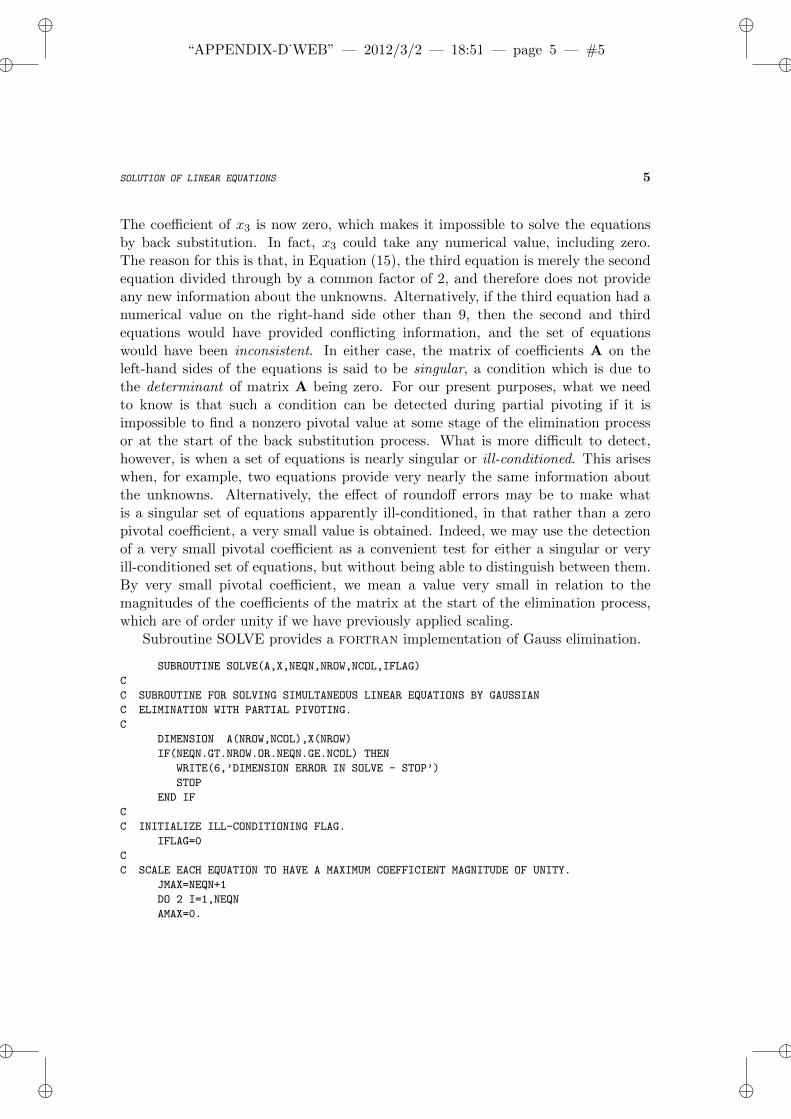
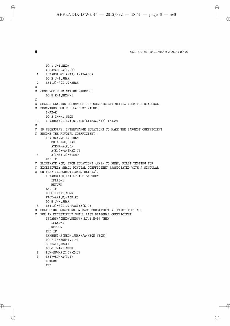
Subroutine SOLVE provides a fortran implementation of Gauss elimination.
SUBROUTINE SOLVE(A,X,NEQN,NROW,NCOL,IFLAG)
C
C SUBROUTINE FOR SOLVING SIMULTANEOUS LINEAR EQUATIONS BY GAUSSIAN
C ELIMINATION WITH PARTIAL PIVOTING.
C
DIMENSION A(NROW,NCOL),X(NROW)
IF(NEQN.GT.NROW.OR.NEQN.GE.NCOL) THEN
WRITE(6,’DIMENSION ERROR IN SOLVE - STOP’)
STOP
END IF
C
C INITIALIZE ILL-CONDITIONING FLAG.
IFLAG=0
C
C SCALE EACH EQUATION TO HAVE A MAXIMUM COEFFICIENT MAGNITUDE OF UNITY.
JMAX=NEQN+1
DO 2 I=1,NEQN
AMAX=0.
ii
“APPENDIX-D˙WEB” — 2012/3/2 — 18:51 — page 6 — #6 ii
ii
ii
6 SOLUTION OF LINEAR EQUATIONS
DO 1 J=1,NEQN
ABSA=ABS(A(I,J))
1 IF(ABSA.GT.AMAX) AMAX=ABSA
DO 2 J=1,JMAX
2 A(I,J)=A(I,J)/AMAX
C
C COMMENCE ELIMINATION PROCESS.
DO 5 K=1,NEQN-1
C
C SEARCH LEADING COLUMN OF THE COEFFICIENT MATRIX FROM THE DIAGONAL
C DOWNWARDS FOR THE LARGEST VALUE.
IMAX=K
DO 3 I=K+1,NEQN
3 IF(ABS(A(I,K)).GT.ABS(A(IMAX,K))) IMAX=I
C
C IF NECESSARY, INTERCHANGE EQUATIONS TO MAKE THE LARGEST COEFFICIENT
C BECOME THE PIVOTAL COEFFICIENT.
IF(IMAX.NE.K) THEN
DO 4 J=K,JMAX
ATEMP=A(K,J)
A(K,J)=A(IMAX,J)
4 A(IMAX,J)=ATEMP
END IF
C ELIMINATE X(K) FROM EQUATIONS (K+1) TO NEQN, FIRST TESTING FOR
C EXCESSIVELY SMALL PIVOTAL COEFFICIENT (ASSOCIATED WITH A SINGULAR
C OR VERY ILL-CONDITIONED MATRIX).
IF(ABS(A(K,K)).LT.1.E-5) THEN
IFLAG=1
RETURN
END IF
DO 5 I=K+1,NEQN
FACT=A(I,K)/A(K,K)
DO 5 J=K,JMAX
5 A(I,J)=A(I,J)-FACT*A(K,J)
C SOLVE THE EQUATIONS BY BACK SUBSTITUTION, FIRST TESTING
C FOR AN EXCESSIVELY SMALL LAST DIAGONAL COEFFICIENT.
IF(ABS(A(NEQN,NEQN)).LT.1.E-5) THEN
IFLAG=1
RETURN
END IF
X(NEQN)=A(NEQN,JMAX)/A(NEQN,NEQN)
DO 7 I=NEQN-1,1,-1
SUM=A(I,JMAX)
DO 6 J=I+1,NEQN
6 SUM=SUM-A(I,J)*X(J)
7 X(I)=SUM/A(I,I)
RETURN
END
ii
“APPENDIX-D˙WEB” — 2012/3/2 — 18:51 — page 7 — #7 ii
ii
ii
SOLUTION OF LINEAR EQUATIONS 7
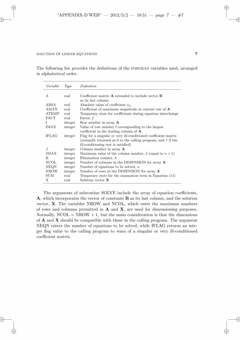
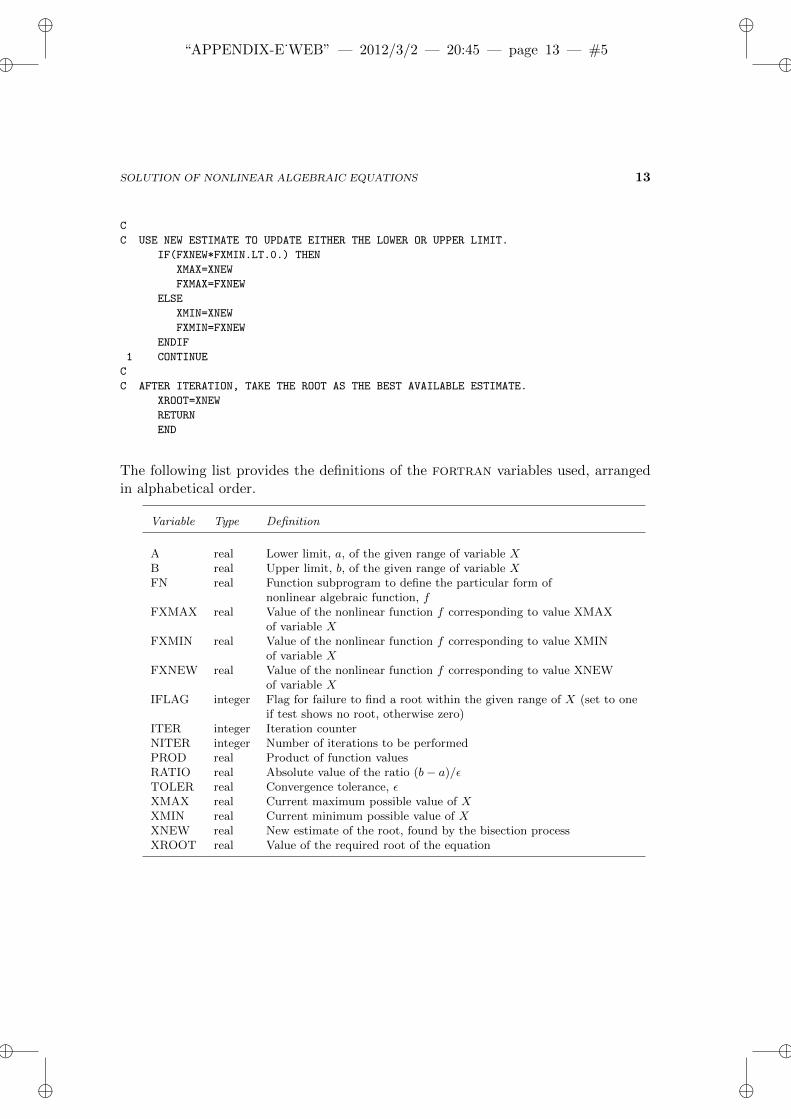
The following list provides the definitions of the fortran variables used, arrangedin alphabetical order.
Variable Type Definition
A real Coefficient matrix A extended to include vector Bas its last column
ABSA real Absolute value of coefficient aij
AMAX real Coefficient of maximum magnitude in current row of AATEMP real Temporary store for coefficients during equation interchangeFACT real Factor fI integer Row number in array AIMAX integer Value of row number I corresponding to the largest
coefficient in the leading column of AIFLAG integer Flag for a singular or very ill-conditioned coefficient matrix
(normally returned as 0 to the calling program, and 1 if theill-conditioning test is satisfied)
J integer Column number in array AJMAX integer Maximum value of the column number, J (equal to n + 1)K integer Elimination counter, kNCOL integer Number of columns in the DIMENSION for array ANEQN integer Number of equations to be solved, nNROW integer Number of rows in the DIMENSION for array ASUM real Temporary store for the summation term in Equation (11)X real Solution vector X
The arguments of subroutine SOLVE include the array of equation coefficients,A, which incorporates the vector of constants B as its last column, and the solutionvector, X. The variables NROW and NCOL, which enter the maximum numbersof rows and columns permitted in A and X, are used for dimensioning purposes.Normally, NCOL = NROW + 1, but the main consideration is that the dimensionsof A and X should be compatible with those in the calling program. The argumentNEQN enters the number of equations to be solved, while IFLAG returns an inte-ger flag value to the calling program to warn of a singular or very ill-conditionedcoefficient matrix.
ii
“APPENDIX-D˙WEB” — 2012/3/2 — 18:51 — page 8 — #8 ii
ii
ii
8 SOLUTION OF LINEAR EQUATIONS
The first action of the program is to test the acceptability of the number ofequations to be solved, in relation to the maximum array sizes. Then IFLAG is setto zero, before the equations are scaled to give a maximum coefficient magnitude ofunity in each row of A. The elimination process is then started: each equation, withthe exception of the last, is used in turn to eliminate the corresponding unknownfrom the subsequent equations. The current elimination number is given by K, andis equivalent to k in Equation (8). Before performing the necessary eliminationswith a particular equation, however, a search is made down the leading column ofthe remaining submatrix to find the coefficient of greatest magnitude, as defined byEquation (12). The search technique locates the row number of the largest coefficient,IMAX, by first assuming that it corresponds to the coefficient on the diagonal, andonly changing this if a larger coefficient is found. If the pivotal coefficient is not thelargest, the relevant equations are interchanged by interchanging all their coefficients.In computing terms, this movement of data between storage locations is inefficient.While it could be avoided by keeping a record of the revised order in which theequations are to be considered, this makes the program significantly more difficultto understand. For present purposes, we sacrifice computational efficiency in theinterests of clarity, in the knowledge that for the relatively small sets of equationswe wish to solve, the extra computing time involved is very small.
Despite the search for the largest coefficient, it is still possible for the pivotalcoefficient to be extremely small or zero if the coefficient matrix is singular or very ill-conditioned. Bearing in mind that the equations were scaled initially, an appropriatetest of magnitude on a computer working to 32 bit precision for real variables is
|akk| < 10−5 (18)
If this condition is satisfied at any stage of the elimination process, the problem isrejected. Rejection is indicated by setting the value of IFLAG to one, which may bedetected by the calling program. If the partial pivoting is successful, however, theeliminations defined by Equation (8) are performed, with the variable FACT beingused to store the values of the factor f .
After testing the magnitude of the last diagonal coefficient [a(n)nn in Equation (9)],
the back substitutions defined in Equations (10) and (11) are performed to findthe required solutions. The variable SUM is used to accumulate the results of thesummations indicated in Equation (11).
ii
“APPENDIX-E˙WEB” — 2012/3/2 — 20:45 — page 9 — #1 ii
ii
ii
9
Solution of Nonlinear AlgebraicEquations
Nonlinear algebraic equations arise in the analysis of many different problems inengineering. In this book we meet examples of polynomial equations in the treat-ment of beam deflection problems, and equations involving trigonometric functionsin the analysis of buckling problems. Any nonlinear algebraic equation with a singlevariable can be expressed in the form
f(X) = 0 (1)
where f(X) is some nonlinear function of the variable X. Consider, for example, thecase arising in Example 6.8, Equation (6.51)
0.12X2 − 1
6(X − 0.2)3 − 0.024 = 0 (2)
The object of solving such an equation is to find a value of X which satisfies theequation. This value is said to be a root of the equation. Now, in general an equationin the form of (1) may have an arbitrarily large number of real roots (real as opposedto imaginary or complex): a cubic equation such as (2), may have as many as threereal roots. In practice, however, we are usually interested in only one of the roots,which we can often identify from the nature of the physical problem from which theequation is derived. In the case of Equation (2), for instance, we seek a root in therange 0.2 < X < 0.6, and we expect there to be only one root in that range.
Many different methods have been developed for solving nonlinear algebraic equa-tions, and are described in detail in numerical analysis textbooks. All are iterative innature: we first guess a value for the required root and then repeatedly obtain suc-cessively better values until one which is sufficiently close to the true root is achieved.Two properties of iterative methods are of great importance: the rate of convergence,which determines how fast the required root is approached, and the stability, whichdetermines whether the root is approached at all, or whether successive estimatesdiverge from the root. Unfortunately, those methods which show good rates of con-vergence under favorable conditions also tend to be the most unstable under adverseconditions. The best choice of method therefore depends on the conditions under
ii
“APPENDIX-E˙WEB” — 2012/3/2 — 20:45 — page 10 — #2 ii
ii
ii
10 SOLUTION OF NONLINEAR ALGEBRAIC EQUATIONS
which it is to be used. If an equation is to be solved manually, then calculations areexpensive and the rate of convergence is important. Any tendency towards unstablebehavior can be rapidly detected and action taken. On the other hand, if an equa-tion is to be solved using a computer, calculations are cheap but more difficult tomonitor and control: stability of the method is then more important than its rate ofconvergence.
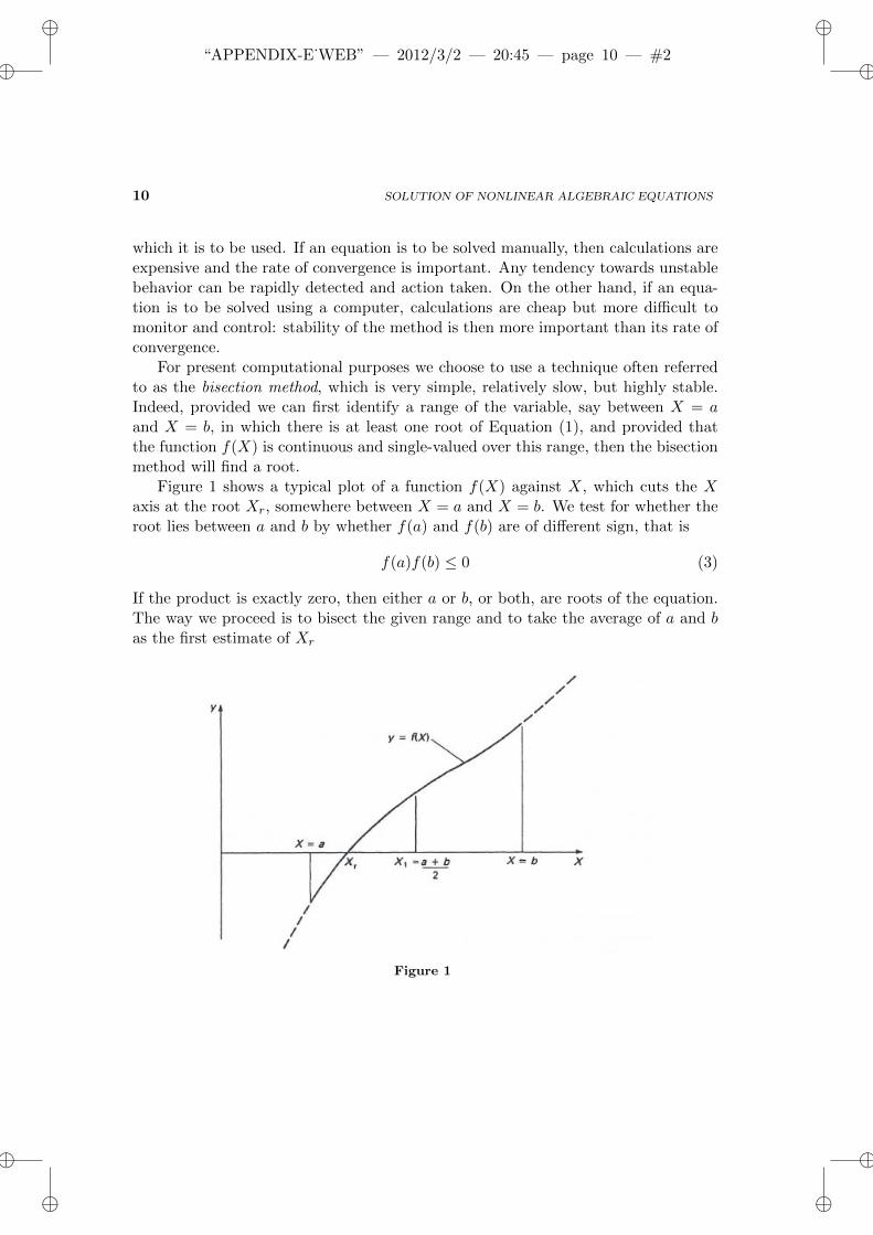
For present computational purposes we choose to use a technique often referredto as the bisection method, which is very simple, relatively slow, but highly stable.Indeed, provided we can first identify a range of the variable, say between X = aand X = b, in which there is at least one root of Equation (1), and provided thatthe function f(X) is continuous and single-valued over this range, then the bisectionmethod will find a root.
Figure 1 shows a typical plot of a function f(X) against X, which cuts the Xaxis at the root Xr, somewhere between X = a and X = b. We test for whether theroot lies between a and b by whether f(a) and f(b) are of different sign, that is
f(a)f(b) ≤ 0 (3)
If the product is exactly zero, then either a or b, or both, are roots of the equation.The way we proceed is to bisect the given range and to take the average of a and bas the first estimate of Xr
Figure 1
ii
“APPENDIX-E˙WEB” — 2012/3/2 — 20:45 — page 11 — #3 ii
ii
ii
SOLUTION OF NONLINEAR ALGEBRAIC EQUATIONS 11
X1 =a+ b
2(4)
We then test (by the same function product method) whether the root lies in theleft-hand or right-hand half of the original range, and adjust either the upper or lowerlimit of the range accordingly. For example, if the product f(a)f(X1) is negativethen X1 replaces b as the upper limit The method is then applied repeatedly, eachtime halving the range of X in which the root must lie, thereby slowly but surelyconverging to this root.
Given a set of estimates of the required root, X1, X2, X3 . . . and so on, we mustdecide when we are sufficiently close to the true value so that the iterative processcan be stopped. To do this, we test the difference between successive estimates,Xi − Xi−1, and require that this be less than some small tolerance, say ε. Undercertain circumstances, we might prefer to test the magnitude of the difference relativeto the magnitude of the root, say (Xi −Xi−1)/Xi, but this is potentially hazardousas Xi might be zero, and computers normally reject division by zero. Because ofthe very simple nature of the bisection method, we are able to predict in advancehow many iterations will be required to achieve convergence to a given tolerance.Taking the initial estimate for the root as either a or b, the first iteration, definedby Equation (4), gives a new estimate which differs by (b − a)/2 from the initialone. After the second iteration, the difference is halved at (b− a)/22. Every furtheriteration halves the difference, until after n iterations it is (b − a)/2n, and in orderto achieve convergence to the given tolerance we require that
|b− a|2n
< ε (5)
from which we can define the number of iterations required as
n =ln|(b− a)/ε|
ln2(6)
In general this equation does not give an integer value for n, and the value obtainedshould be rounded up to the next integer to satisfy inequality (5).
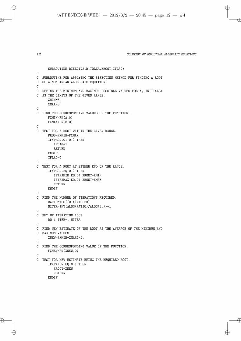
Subroutine BISECT provides a fortran implementation of the bisection method.
ii
“APPENDIX-E˙WEB” — 2012/3/2 — 20:45 — page 12 — #4 ii
ii
ii
12 SOLUTION OF NONLINEAR ALGEBRAIC EQUATIONS
SUBROUTINE BISECT(A,B,TOLER,XROOT,IFLAG)
C
C SUBROUTINE FOR APPLYING THE BISECTION METHOD FOR FINDING A ROOT
C OF A NONLINEAR ALGEBRAIC EQUATION.
C
C DEFINE THE MINIMUM AND MAXIMUM POSSIBLE VALUES FOR X, INITIALLY
C AS THE LIMITS OF THE GIVEN RANGE.
XMIN=A
XMAX=B
C
C FIND THE CORRESPONDING VALUES OF THE FUNCTION.
FXMIN=FN(A,0)
FXMAX=FN(B,0)
C
C TEST FOR A ROOT WITHIN THE GIVEN RANGE.
PROD=FXMIN*FXMAX
IF(PROD.GT.0.) THEN
IFLAG=1
RETURN
ENDIF
IFLAG=0
C
C TEST FOR A ROOT AT EITHER END OF THE RANGE.
IF(PROD.EQ.0.) THEN
IF(FXMIN.EQ.0) XROOT=XMIN
IF(FXMAX.EQ.0) XROOT=XMAX
RETURN
ENDIF
C
C FIND THE NUMBER OF ITERATIONS REQUIRED.
RATIO=ABS((B-A)/TOLER)
NITER=INT(ALOG(RATIO)/ALOG(2.))+1
C
C SET UP ITERATION LOOP.
DO 1 ITER=1,NITER
C
C FIND NEW ESTIMATE OF THE ROOT AS THE AVERAGE OF THE MINIMUM AND
C MAXIMUM VALUES.
XNEW=(XMIN+XMAX)/2.
C
C FIND THE CORRESPONDING VALUE OF THE FUNCTION.
FXNEW=FN(XNEW,0)
C
C TEST FOR NEW ESTIMATE BEING THE REQUIRED ROOT.
IF(FXNEW.EQ.0.) THEN
XROOT=XNEW
RETURN
ENDIF
ii
“APPENDIX-E˙WEB” — 2012/3/2 — 20:45 — page 13 — #5 ii
ii
ii
SOLUTION OF NONLINEAR ALGEBRAIC EQUATIONS 13
C
C USE NEW ESTIMATE TO UPDATE EITHER THE LOWER OR UPPER LIMIT.
IF(FXNEW*FXMIN.LT.0.) THEN
XMAX=XNEW
FXMAX=FXNEW
ELSE
XMIN=XNEW
FXMIN=FXNEW
ENDIF
1 CONTINUE
C
C AFTER ITERATION, TAKE THE ROOT AS THE BEST AVAILABLE ESTIMATE.
XROOT=XNEW
RETURN
END
The following list provides the definitions of the fortran variables used, arrangedin alphabetical order.
Variable Type Definition
A real Lower limit, a, of the given range of variable XB real Upper limit, b, of the given range of variable XFN real Function subprogram to define the particular form of
nonlinear algebraic function, fFXMAX real Value of the nonlinear function f corresponding to value XMAX
of variable XFXMIN real Value of the nonlinear function f corresponding to value XMIN
of variable XFXNEW real Value of the nonlinear function f corresponding to value XNEW
of variable XIFLAG integer Flag for failure to find a root within the given range of X (set to one
if test shows no root, otherwise zero)ITER integer Iteration counterNITER integer Number of iterations to be performedPROD real Product of function valuesRATIO real Absolute value of the ratio (b− a)/εTOLER real Convergence tolerance, εXMAX real Current maximum possible value of XXMIN real Current minimum possible value of XXNEW real New estimate of the root, found by the bisection processXROOT real Value of the required root of the equation
ii
“APPENDIX-E˙WEB” — 2012/3/2 — 20:45 — page 14 — #6 ii
ii
ii
14 SOLUTION OF NONLINEAR ALGEBRAIC EQUATIONS
The arguments of subroutine BISECT are the given limits, A and B, of the possiblerange for the root, the convergence tolerance, TOLER, the computed value of theroot, XROOT, and the variable IFLAG. While the first three of these provide datato the subroutine, the last two provide the results, the last one returning an integerflag value to the calling program to warn of no root in the given range.
The first action of the subroutine is to compute the values of the nonlinear func-tion, f in Equation (1), corresponding to the given limits of the possible range for X.This is done using a further function subprogram, FN, whose form must be suitedto the particular equation being solved. The reason for having two arguments forthis subprogram, the value of X and another integer quantity (here set to zero), isexplained below. We test for a root within the given range by testing the product ofthe two function values. A positive value of the product indicates that there is not asingle root in the range (although for a continuous function there could be an evennumber of roots), and a zero value indicates that either a or b (or both) must be aroot.
The number of iterations is then computed with the aid of Equation (6) (notethat, since fortran function INT truncates its argument to the integer immediatelybelow it, one is added to obtain the integer immediately above it). An iterationloop is then set up to bisect repeatedly the possible range for the root. If one ofthe resulting estimates for the root should happen to exactly satisfy the nonlinearequation, this value is returned as the root to the calling program. Otherwise, thevalue obtained from the last iteration is taken as the root.
Now, subroutine BISECT is designed as a piece of coding for applying the bisec-tion method which is independent of both the particular nonlinear equation to besolved and the program which requires the solution. It can therefore be used in anysituation where such an equation has to be solved, including, for example, programsibeam which is described in Section 6.4.2. Similarly, it can be used to solve thecubic equation derived in Example 6.8, which is repeated here in Equation (2). Todo this, we must prepare a small main program, and an appropriate form of functionsubprogram FN.
Program root provides the main program for entering the data for solving anonlinear algebraic equation. After writing out an appropriate title onto an outputfile named RESULTS, root calls function subprogram FN to also write out the formof nonlinear equation being solved. The values of a, b, and ε are then read in froman input file named DATA, and immediately written out, and subroutine BISECTis called to solve the equation. The computed results are written out, either in theform of the computed root or a warning message that there is no single solutionwithin the given range.
ii
“APPENDIX-E˙WEB” — 2012/3/2 — 20:45 — page 15 — #7 ii
ii
ii
SOLUTION OF NONLINEAR ALGEBRAIC EQUATIONS 15
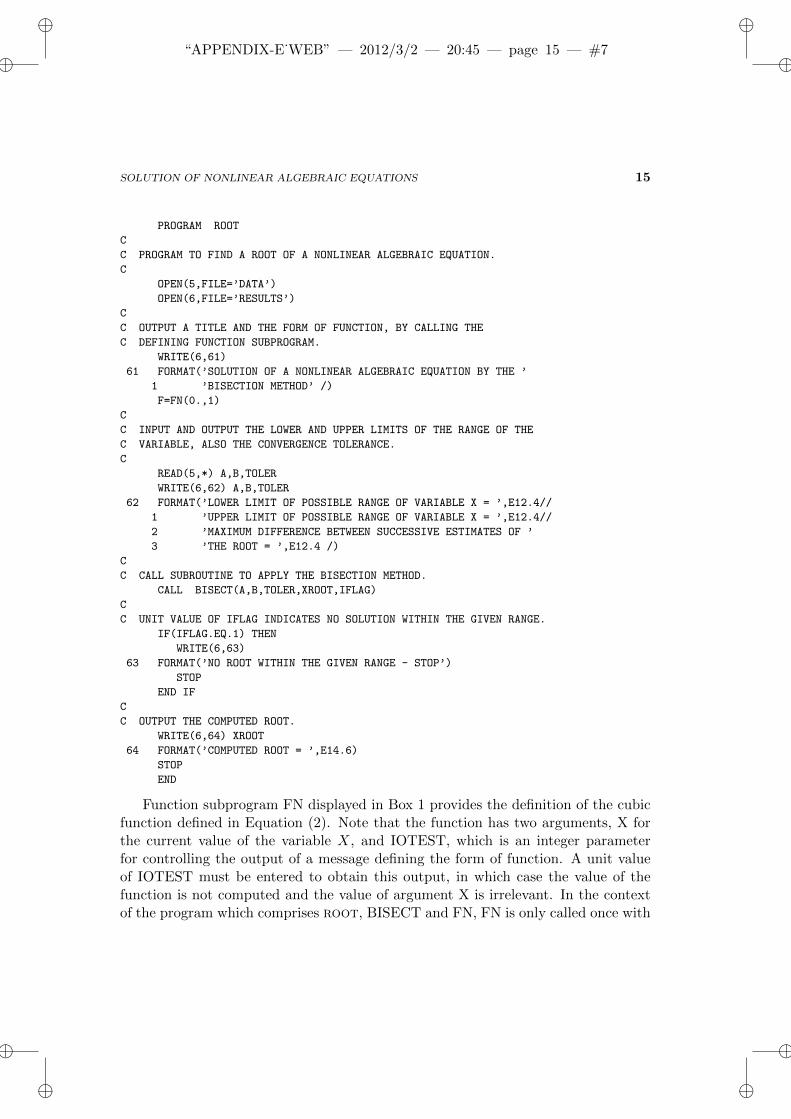
PROGRAM ROOT
C
C PROGRAM TO FIND A ROOT OF A NONLINEAR ALGEBRAIC EQUATION.
C
OPEN(5,FILE=’DATA’)
OPEN(6,FILE=’RESULTS’)
C
C OUTPUT A TITLE AND THE FORM OF FUNCTION, BY CALLING THE
C DEFINING FUNCTION SUBPROGRAM.
WRITE(6,61)
61 FORMAT(’SOLUTION OF A NONLINEAR ALGEBRAIC EQUATION BY THE ’
1 ’BISECTION METHOD’ /)
F=FN(0.,1)
C
C INPUT AND OUTPUT THE LOWER AND UPPER LIMITS OF THE RANGE OF THE
C VARIABLE, ALSO THE CONVERGENCE TOLERANCE.
C
READ(5,*) A,B,TOLER
WRITE(6,62) A,B,TOLER
62 FORMAT(’LOWER LIMIT OF POSSIBLE RANGE OF VARIABLE X = ’,E12.4//
1 ’UPPER LIMIT OF POSSIBLE RANGE OF VARIABLE X = ’,E12.4//
2 ’MAXIMUM DIFFERENCE BETWEEN SUCCESSIVE ESTIMATES OF ’
3 ’THE ROOT = ’,E12.4 /)
C
C CALL SUBROUTINE TO APPLY THE BISECTION METHOD.
CALL BISECT(A,B,TOLER,XROOT,IFLAG)
C
C UNIT VALUE OF IFLAG INDICATES NO SOLUTION WITHIN THE GIVEN RANGE.
IF(IFLAG.EQ.1) THEN
WRITE(6,63)
63 FORMAT(’NO ROOT WITHIN THE GIVEN RANGE - STOP’)
STOP
END IF
C
C OUTPUT THE COMPUTED ROOT.
WRITE(6,64) XROOT
64 FORMAT(’COMPUTED ROOT = ’,E14.6)
STOP
END
Function subprogram FN displayed in Box 1 provides the definition of the cubicfunction defined in Equation (2). Note that the function has two arguments, X forthe current value of the variable X, and IOTEST, which is an integer parameterfor controlling the output of a message defining the form of function. A unit valueof IOTEST must be entered to obtain this output, in which case the value of thefunction is not computed and the value of argument X is irrelevant. In the contextof the program which comprises root, BISECT and FN, FN is only called once with
ii
“APPENDIX-E˙WEB” — 2012/3/2 — 20:45 — page 16 — #8 ii
ii
ii
16 SOLUTION OF NONLINEAR ALGEBRAIC EQUATIONS
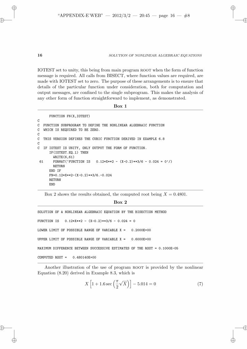
IOTEST set to unity, this being from main program root when the form of functionmessage is required. All calls from BISECT, where function values are required, aremade with IOTEST set to zero. The purpose of these arrangements is to ensure thatdetails of the particular function under consideration, both for computation andoutput messages, are confined to the single subprogram. This makes the analysis ofany other form of function straightforward to implement, as demonstrated.
Box 1
FUNCTION FN(X,IOTEST)
C
C FUNCTION SUBPROGRAM TO DEFINE THE NONLINEAR ALGEBRAIC FUNCTION
C WHICH IS REQUIRED TO BE ZERO.
C
C THIS VERSION DEFINES THE CUBIC FUNCTION DERIVED IN EXAMPLE 6.8
C
C IF IOTEST IS UNITY, ONLY OUTPUT THE FORM OF FUNCTION.
IF(IOTEST.EQ.l) THEN
WRITE(6,61)
61 FORMAT(‘FUNCTION IS 0.12*X**2 - (X-0.2)**3/6 - 0.024 = 0’/)
RETURN
END IF
FN=0.12*X**2-(X-0.2)**3/6.-0.024
RETURN
END
Box 2 shows the results obtained, the computed root being X = 0.4801.
Box 2
SOLUTION OF A NONLINEAR ALGEBRAIC EQUATION BY THE BISECTION METHOD
FUNCTION IS 0.12*X**2 - (X-0.2)**3/6 - 0.024 = 0
LOWER LIMIT OF POSSIBLE RANGE OF VARIABLE X = 0.2000E+00
UPPER LIMIT OF POSSIBLE RANGE OF VARIABLE X = 0.6000E+00
MAXIMUM DIFFERENCE BETWEEN SUCCESSIVE ESTIMATES OF THE ROOT = 0.1000E-05
COMPUTED ROOT = 0.480140E+00
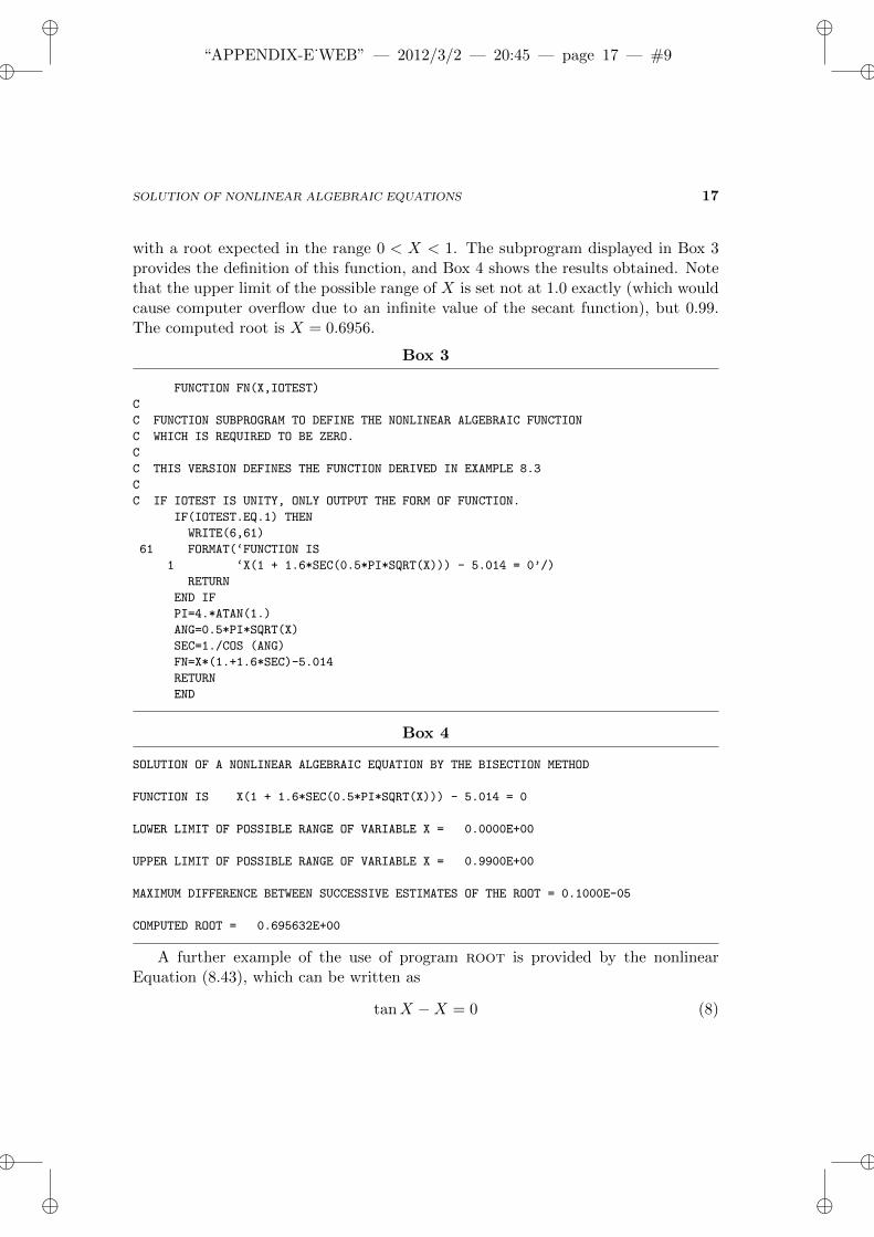
Another illustration of the use of program root is provided by the nonlinearEquation (8.20) derived in Example 8.3, which is
X[1 + 1.6 sec
(π2
√X)]− 5.014 = 0 (7)
ii
“APPENDIX-E˙WEB” — 2012/3/2 — 20:45 — page 17 — #9 ii
ii
ii
SOLUTION OF NONLINEAR ALGEBRAIC EQUATIONS 17
with a root expected in the range 0 < X < 1. The subprogram displayed in Box 3provides the definition of this function, and Box 4 shows the results obtained. Notethat the upper limit of the possible range of X is set not at 1.0 exactly (which wouldcause computer overflow due to an infinite value of the secant function), but 0.99.The computed root is X = 0.6956.
Box 3
FUNCTION FN(X,IOTEST)
C
C FUNCTION SUBPROGRAM TO DEFINE THE NONLINEAR ALGEBRAIC FUNCTION
C WHICH IS REQUIRED TO BE ZERO.
C
C THIS VERSION DEFINES THE FUNCTION DERIVED IN EXAMPLE 8.3
C
C IF IOTEST IS UNITY, ONLY OUTPUT THE FORM OF FUNCTION.
IF(IOTEST.EQ.1) THEN
WRITE(6,61)
61 FORMAT(‘FUNCTION IS
1 ‘X(1 + 1.6*SEC(0.5*PI*SQRT(X))) - 5.014 = 0’/)
RETURN
END IF
PI=4.*ATAN(1.)
ANG=0.5*PI*SQRT(X)
SEC=1./COS (ANG)
FN=X*(1.+1.6*SEC)-5.014
RETURN
END
Box 4
SOLUTION OF A NONLINEAR ALGEBRAIC EQUATION BY THE BISECTION METHOD
FUNCTION IS X(1 + 1.6*SEC(0.5*PI*SQRT(X))) - 5.014 = 0
LOWER LIMIT OF POSSIBLE RANGE OF VARIABLE X = 0.0000E+00
UPPER LIMIT OF POSSIBLE RANGE OF VARIABLE X = 0.9900E+00
MAXIMUM DIFFERENCE BETWEEN SUCCESSIVE ESTIMATES OF THE ROOT = 0.1000E-05
COMPUTED ROOT = 0.695632E+00
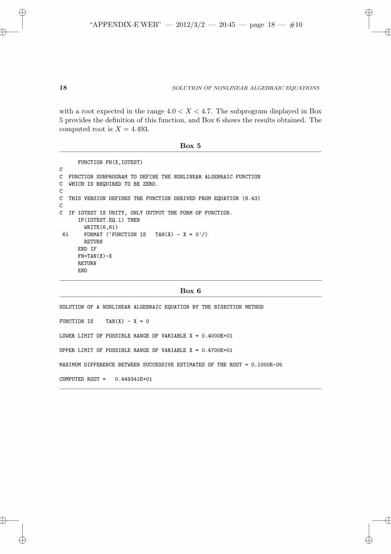
A further example of the use of program root is provided by the nonlinearEquation (8.43), which can be written as
tanX −X = 0 (8)
ii
“APPENDIX-E˙WEB” — 2012/3/2 — 20:45 — page 18 — #10 ii
ii
ii
18 SOLUTION OF NONLINEAR ALGEBRAIC EQUATIONS
with a root expected in the range 4.0 < X < 4.7. The subprogram displayed in Box5 provides the definition of this function, and Box 6 shows the results obtained. Thecomputed root is X = 4.493.
Box 5
FUNCTION FN(X,IOTEST)
C
C FUNCTION SUBPROGRAM TO DEFINE THE NONLINEAR ALGEBRAIC FUNCTION
C WHICH IS REQUIRED TO BE ZERO.
C
C THIS VERSION DEFINES THE FUNCTION DERIVED FROM EQUATION (8.43)
C
C IF IOTEST IS UNITY, ONLY OUTPUT THE FORM OF FUNCTION.
IF(IOTEST.EQ.l) THEN
WRITE(6,61)
61 FORMAT (‘FUNCTION IS TAN(X) - X = 0’/)
RETURN
END IF
FN=TAN(X)-X
RETURN
END
Box 6
SOLUTION OF A NONLINEAR ALGEBRAIC EQUATION BY THE BISECTION METHOD
FUNCTION IS TAN(X) - X = 0
LOWER LIMIT OF POSSIBLE RANGE OF VARIABLE X = 0.4000E+01
UPPER LIMIT OF POSSIBLE RANGE OF VARIABLE X = 0.4700E+01
MAXIMUM DIFFERENCE BETWEEN SUCCESSIVE ESTIMATES OF THE ROOT = 0.1000E-05
COMPUTED ROOT = 0.449341E+01
ii
“APPENDIX-F˙WEB” — 2012/3/2 — 20:47 — page 19 — #1 ii
ii
ii
19
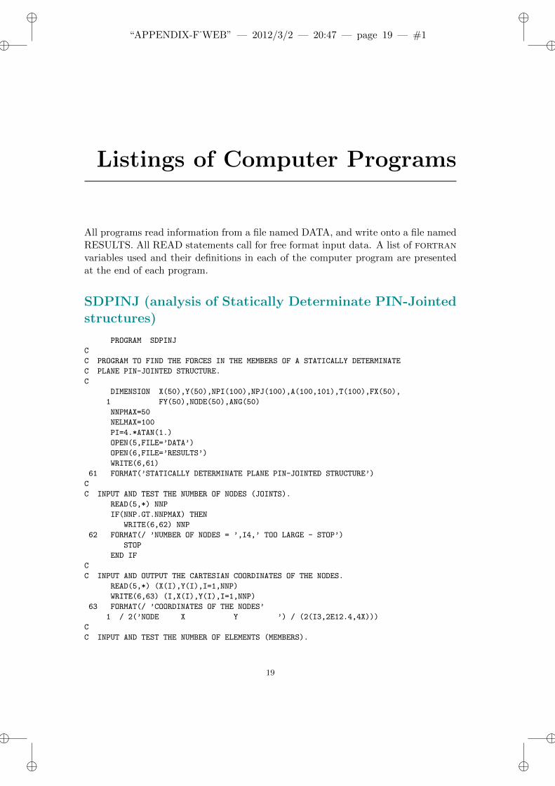
Listings of Computer Programs
All programs read information from a file named DATA, and write onto a file namedRESULTS. All READ statements call for free format input data. A list of fortranvariables used and their definitions in each of the computer program are presentedat the end of each program.
SDPINJ (analysis of Statically Determinate PIN-Jointedstructures)
PROGRAM SDPINJ
C
C PROGRAM TO FIND THE FORCES IN THE MEMBERS OF A STATICALLY DETERMINATE
C PLANE PIN-JOINTED STRUCTURE.
C
DIMENSION X(50),Y(50),NPI(100),NPJ(100),A(100,101),T(100),FX(50),
1 FY(50),NODE(50),ANG(50)
NNPMAX=50
NELMAX=100
PI=4.*ATAN(1.)
OPEN(5,FILE=’DATA’)
OPEN(6,FILE=’RESULTS’)
WRITE(6,61)
61 FORMAT(’STATICALLY DETERMINATE PLANE PIN-JOINTED STRUCTURE’)
C
C INPUT AND TEST THE NUMBER OF NODES (JOINTS).
READ(5,*) NNP
IF(NNP.GT.NNPMAX) THEN
WRITE(6,62) NNP
62 FORMAT(/ ’NUMBER OF NODES = ’,I4,’ TOO LARGE - STOP’)
STOP
END IF
C
C INPUT AND OUTPUT THE CARTESIAN COORDINATES OF THE NODES.
READ(5,*) (X(I),Y(I),I=1,NNP)
WRITE(6,63) (I,X(I),Y(I),I=1,NNP)
63 FORMAT(/ ’COORDINATES OF THE NODES’
1 / 2(’NODE X Y ’) / (2(I3,2E12.4,4X)))
C
C INPUT AND TEST THE NUMBER OF ELEMENTS (MEMBERS).
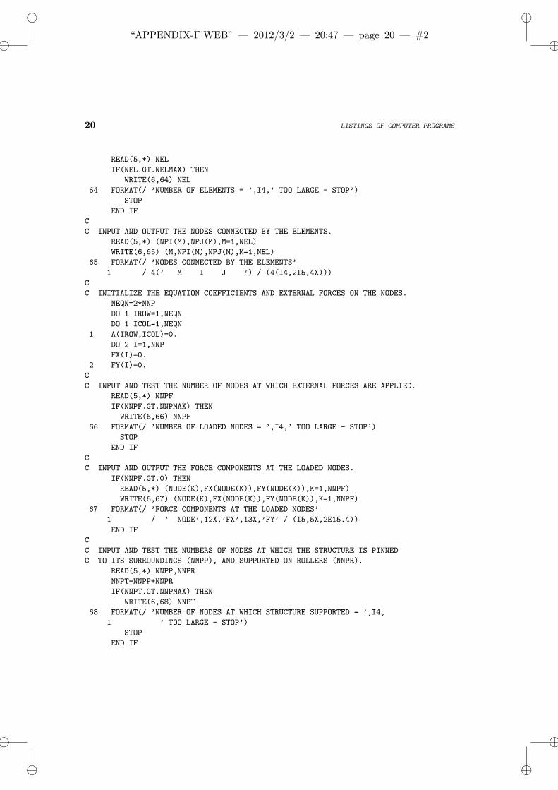
ii
“APPENDIX-F˙WEB” — 2012/3/2 — 20:47 — page 20 — #2 ii
ii
ii
20 LISTINGS OF COMPUTER PROGRAMS
READ(5,*) NEL
IF(NEL.GT.NELMAX) THEN
WRITE(6,64) NEL
64 FORMAT(/ ’NUMBER OF ELEMENTS = ’,I4,’ TOO LARGE - STOP’)
STOP
END IF
C
C INPUT AND OUTPUT THE NODES CONNECTED BY THE ELEMENTS.
READ(5,*) (NPI(M),NPJ(M),M=1,NEL)
WRITE(6,65) (M,NPI(M),NPJ(M),M=1,NEL)
65 FORMAT(/ ’NODES CONNECTED BY THE ELEMENTS’
1 / 4(’ M I J ’) / (4(I4,2I5,4X)))
C
C INITIALIZE THE EQUATION COEFFICIENTS AND EXTERNAL FORCES ON THE NODES.
NEQN=2*NNP
DO 1 IROW=1,NEQN
DO 1 ICOL=1,NEQN
1 A(IROW,ICOL)=0.
DO 2 I=1,NNP
FX(I)=0.
2 FY(I)=0.
C
C INPUT AND TEST THE NUMBER OF NODES AT WHICH EXTERNAL FORCES ARE APPLIED.
READ(5,*) NNPF
IF(NNPF.GT.NNPMAX) THEN
WRITE(6,66) NNPF
66 FORMAT(/ ’NUMBER OF LOADED NODES = ’,I4,’ TOO LARGE - STOP’)
STOP
END IF
C
C INPUT AND OUTPUT THE FORCE COMPONENTS AT THE LOADED NODES.
IF(NNPF.GT.0) THEN
READ(5,*) (NODE(K),FX(NODE(K)),FY(NODE(K)),K=1,NNPF)
WRITE(6,67) (NODE(K),FX(NODE(K)),FY(NODE(K)),K=1,NNPF)
67 FORMAT(/ ’FORCE COMPONENTS AT THE LOADED NODES’
1 / ’ NODE’,12X,’FX’,13X,’FY’ / (I5,5X,2E15.4))
END IF
C
C INPUT AND TEST THE NUMBERS OF NODES AT WHICH THE STRUCTURE IS PINNED
C TO ITS SURROUNDINGS (NNPP), AND SUPPORTED ON ROLLERS (NNPR).
READ(5,*) NNPP,NNPR
NNPT=NNPP+NNPR
IF(NNPT.GT.NNPMAX) THEN
WRITE(6,68) NNPT
68 FORMAT(/ ’NUMBER OF NODES AT WHICH STRUCTURE SUPPORTED = ’,I4,
1 ’ TOO LARGE - STOP’)
STOP
END IF
ii
“APPENDIX-F˙WEB” — 2012/3/2 — 20:47 — page 21 — #3 ii
ii
ii
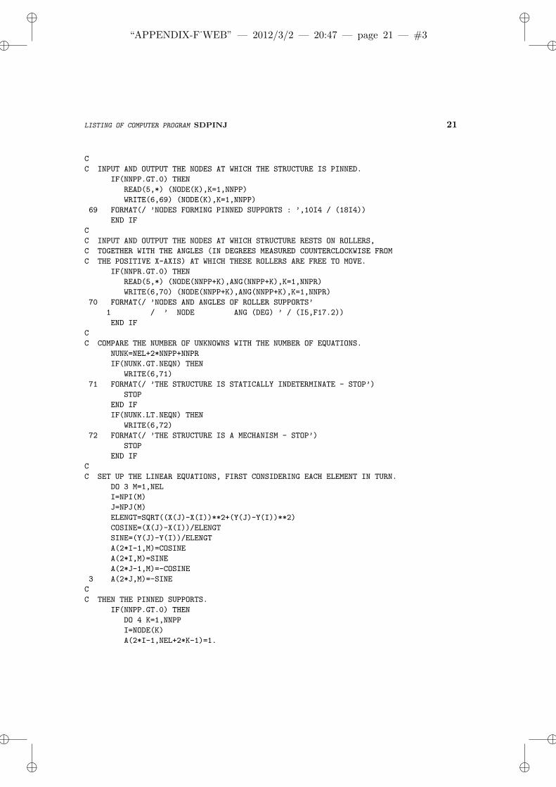
LISTING OF COMPUTER PROGRAM SDPINJ 21
C
C INPUT AND OUTPUT THE NODES AT WHICH THE STRUCTURE IS PINNED.
IF(NNPP.GT.0) THEN
READ(5,*) (NODE(K),K=1,NNPP)
WRITE(6,69) (NODE(K),K=1,NNPP)
69 FORMAT(/ ’NODES FORMING PINNED SUPPORTS : ’,10I4 / (18I4))
END IF
C
C INPUT AND OUTPUT THE NODES AT WHICH STRUCTURE RESTS ON ROLLERS,
C TOGETHER WITH THE ANGLES (IN DEGREES MEASURED COUNTERCLOCKWISE FROM
C THE POSITIVE X-AXIS) AT WHICH THESE ROLLERS ARE FREE TO MOVE.
IF(NNPR.GT.0) THEN
READ(5,*) (NODE(NNPP+K),ANG(NNPP+K),K=1,NNPR)
WRITE(6,70) (NODE(NNPP+K),ANG(NNPP+K),K=1,NNPR)
70 FORMAT(/ ’NODES AND ANGLES OF ROLLER SUPPORTS’
1 / ’ NODE ANG (DEG) ’ / (I5,F17.2))
END IF
C
C COMPARE THE NUMBER OF UNKNOWNS WITH THE NUMBER OF EQUATIONS.
NUNK=NEL+2*NNPP+NNPR
IF(NUNK.GT.NEQN) THEN
WRITE(6,71)
71 FORMAT(/ ’THE STRUCTURE IS STATICALLY INDETERMINATE - STOP’)
STOP
END IF
IF(NUNK.LT.NEQN) THEN
WRITE(6,72)
72 FORMAT(/ ’THE STRUCTURE IS A MECHANISM - STOP’)
STOP
END IF
C
C SET UP THE LINEAR EQUATIONS, FIRST CONSIDERING EACH ELEMENT IN TURN.
DO 3 M=1,NEL
I=NPI(M)
J=NPJ(M)
ELENGT=SQRT((X(J)-X(I))**2+(Y(J)-Y(I))**2)
COSINE=(X(J)-X(I))/ELENGT
SINE=(Y(J)-Y(I))/ELENGT
A(2*I-1,M)=COSINE
A(2*I,M)=SINE
A(2*J-1,M)=-COSINE
3 A(2*J,M)=-SINE
C
C THEN THE PINNED SUPPORTS.
IF(NNPP.GT.0) THEN
DO 4 K=1,NNPP
I=NODE(K)
A(2*I-1,NEL+2*K-1)=1.
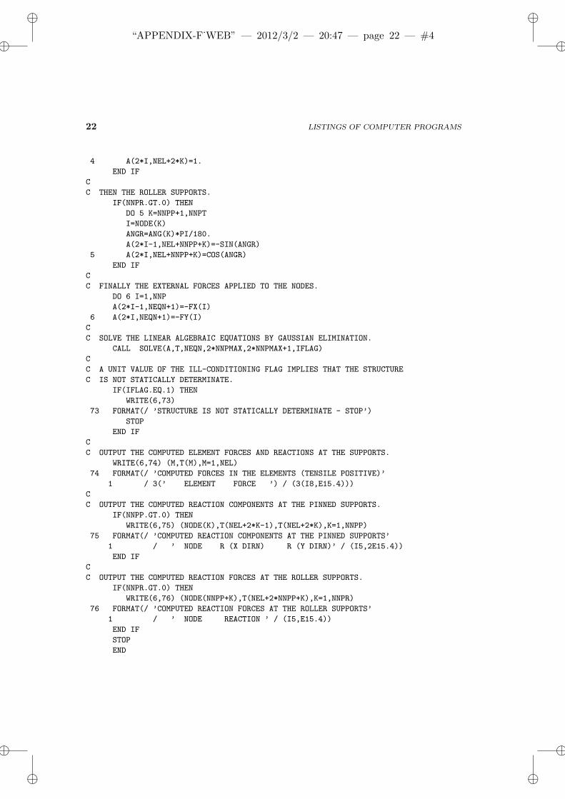
ii
“APPENDIX-F˙WEB” — 2012/3/2 — 20:47 — page 22 — #4 ii
ii
ii
22 LISTINGS OF COMPUTER PROGRAMS
4 A(2*I,NEL+2*K)=1.
END IF
C
C THEN THE ROLLER SUPPORTS.
IF(NNPR.GT.0) THEN
DO 5 K=NNPP+1,NNPT
I=NODE(K)
ANGR=ANG(K)*PI/180.
A(2*I-1,NEL+NNPP+K)=-SIN(ANGR)
5 A(2*I,NEL+NNPP+K)=COS(ANGR)
END IF
C
C FINALLY THE EXTERNAL FORCES APPLIED TO THE NODES.
DO 6 I=1,NNP
A(2*I-1,NEQN+1)=-FX(I)
6 A(2*I,NEQN+1)=-FY(I)
C
C SOLVE THE LINEAR ALGEBRAIC EQUATIONS BY GAUSSIAN ELIMINATION.
CALL SOLVE(A,T,NEQN,2*NNPMAX,2*NNPMAX+1,IFLAG)
C
C A UNIT VALUE OF THE ILL-CONDITIONING FLAG IMPLIES THAT THE STRUCTURE
C IS NOT STATICALLY DETERMINATE.
IF(IFLAG.EQ.1) THEN
WRITE(6,73)
73 FORMAT(/ ’STRUCTURE IS NOT STATICALLY DETERMINATE - STOP’)
STOP
END IF
C
C OUTPUT THE COMPUTED ELEMENT FORCES AND REACTIONS AT THE SUPPORTS.
WRITE(6,74) (M,T(M),M=1,NEL)
74 FORMAT(/ ’COMPUTED FORCES IN THE ELEMENTS (TENSILE POSITIVE)’
1 / 3(’ ELEMENT FORCE ’) / (3(I8,E15.4)))
C
C OUTPUT THE COMPUTED REACTION COMPONENTS AT THE PINNED SUPPORTS.
IF(NNPP.GT.0) THEN
WRITE(6,75) (NODE(K),T(NEL+2*K-1),T(NEL+2*K),K=1,NNPP)
75 FORMAT(/ ’COMPUTED REACTION COMPONENTS AT THE PINNED SUPPORTS’
1 / ’ NODE R (X DIRN) R (Y DIRN)’ / (I5,2E15.4))
END IF
C
C OUTPUT THE COMPUTED REACTION FORCES AT THE ROLLER SUPPORTS.
IF(NNPR.GT.0) THEN
WRITE(6,76) (NODE(NNPP+K),T(NEL+2*NNPP+K),K=1,NNPR)
76 FORMAT(/ ’COMPUTED REACTION FORCES AT THE ROLLER SUPPORTS’
1 / ’ NODE REACTION ’ / (I5,E15.4))
END IF
STOP
END
ii
“APPENDIX-F˙WEB” — 2012/3/2 — 20:47 — page 23 — #5 ii
ii
ii
LISTING OF COMPUTER PROGRAM SDPINJ 23
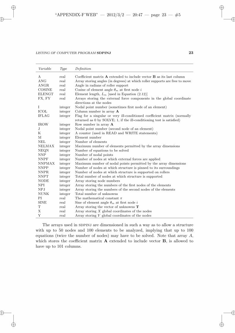
Variable Type Definition
A real Coefficient matrix A extended to include vector B as its last columnANG real Array storing angles (in degrees) at which roller supports are free to moveANGR real Angle in radians of roller supportCOSINE real Cosine of element angle θm at first node iELENGT real Element length, Lm [used in Equation (2.12)]FX, FY real Arrays storing the external force components in the global coordinate
directions at the nodesI integer Nodal point number (sometimes first node of an element)ICOL integer Column number in array AIFLAG integer Flag for a singular or very ill-conditioned coefficient matrix (normally
returned as 0 by SOLVE; 1, if the ill-conditioning test is satisfied)IROW integer Row number in array AJ integer Nodal point number (second node of an element)K integer A counter (used in READ and WRITE statements)M integer Element numberNEL integer Number of elementsNELMAX integer Maximum number of elements permitted by the array dimensionsNEQN integer Number of equations to be solvedNNP integer Number of nodal pointsNNPF integer Number of nodes at which external forces are appliedNNPMAX integer Maximum number of nodal points permitted by the array dimensionsNNPP integer Number of nodes at which structure is pinned to its surroundingsNNPR integer Number of nodes at which structure is supported on rollersNNPT integer Total number of nodes at which structure is supportedNODE integer Array storing node numbersNPI integer Array storing the numbers of the first nodes of the elementsNPJ integer Array storing the numbers of the second nodes of the elementsNUNK integer Total number of unknownsPI real The mathematical constant πSINE real Sine of element angle θm at first node iT real Array storing the vector of unknowns TX real Array storing X global coordinates of the nodesY real Array storing Y global coordinates of the nodes
The arrays used in sdpinj are dimensioned in such a way as to allow a structurewith up to 50 nodes and 100 elements to be analyzed, implying that up to 100equations (twice the number of nodes) may have to be solved. Note that array A,which stores the coefficient matrix A extended to include vector B, is allowed tohave up to 101 columns.
ii
“APPENDIX-F˙WEB” — 2012/3/2 — 20:47 — page 24 — #6 ii
ii
ii
24 LISTINGS OF COMPUTER PROGRAMS
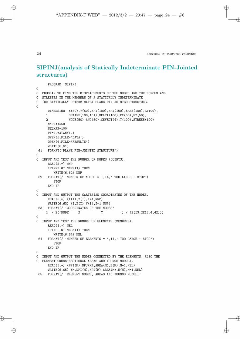
SIPINJ(analysis of Statically Indeterminate PIN-Jointedstructures)
PROGRAM SIPINJ
C
C PROGRAM TO FIND THE DISPLACEMENTS OF THE NODES AND THE FORCES AND
C STRESSES IN THE MEMBERS OF A STATICALLY INDETERMINATE
C (OR STATICALLY DETERMINATE) PLANE PIN-JOINTED STRUCTURE.
C
DIMENSION X(50),Y(50),NPI(100),NPJ(100),AREA(100),E(100),
1 OSTIFF(100,101),DELTA(100),FX(50),FY(50),
2 NODE(50),ANG(50),CSVECT(4),T(100),STRESS(100)
NNPMAX=50
NELMAX=100
PI=4.*ATAN(1.)
OPEN(5,FILE=’DATA’)
OPEN(6,FILE=’RESULTS’)
WRITE(6,61)
61 FORMAT(’PLANE PIN-JOINTED STRUCTURE’)
C
C INPUT AND TEST THE NUMBER OF NODES (JOINTS).
READ(5,*) NNP
IF(NNP.GT.NNPMAX) THEN
WRITE(6,62) NNP
62 FORMAT(/ ’NUMBER OF NODES = ’,I4,’ TOO LARGE - STOP’)
STOP
END IF
C
C INPUT AND OUTPUT THE CARTESIAN COORDINATES OF THE NODES.
READ(5,*) (X(I),Y(I),I=1,NNP)
WRITE(6,63) (I,X(I),Y(I),I=1,NNP)
63 FORMAT(/ ’COORDINATES OF THE NODES’
1 / 2(’NODE X Y ’) / (2(I3,2E12.4,4X)))
C
C INPUT AND TEST THE NUMBER OF ELEMENTS (MEMBERS).
READ(5,*) NEL
IF(NEL.GT.NELMAX) THEN
WRITE(6,64) NEL
64 FORMAT(/ ’NUMBER OF ELEMENTS = ’,I4,’ TOO LARGE - STOP’)
STOP
END IF
C
C INPUT AND OUTPUT THE NODES CONNECTED BY THE ELEMENTS, ALSO THE
C ELEMENT CROSS-SECTIONAL AREAS AND YOUNGS MODULI.
READ(5,*) (NPI(M),NPJ(M),AREA(M),E(M),M=1,NEL)
WRITE(6,65) (M,NPI(M),NPJ(M),AREA(M),E(M),M=1,NEL)
65 FORMAT(/ ’ELEMENT NODES, AREAS AND YOUNGS MODULI’
ii
“APPENDIX-F˙WEB” — 2012/3/2 — 20:47 — page 25 — #7 ii
ii
ii
LISTING OF COMPUTER PROGRAM SIPINJ 25
1 / ’ M I J AREA E’
2 / (I4,2I5,2E15.4))
C
C INITIALIZE THE OVERALL STIFFNESS COEFFICIENTS AND EXTERNAL FORCES
C ON THE NODES.
NEQN=2*NNP
DO 1 IROW=1,NEQN
DO 1 ICOL=1,NEQN
1 OSTIFF(IROW,ICOL)=0.
DO 2 I=1,NNP
FX(I)=0.
2 FY(I)=0.
C
C INPUT AND TEST THE NUMBER OF NODES AT WHICH EXTERNAL FORCES ARE APPLIED.
READ(5,*) NNPF
IF(NNPF.GT.NNPMAX) THEN
WRITE(6,66) NNPF
66 FORMAT(/ ’NUMBER OF LOADED NODES = ’,I4,’ TOO LARGE - STOP’)
STOP
END IF
C
C INPUT AND OUTPUT THE FORCE COMPONENTS AT THE LOADED NODES.
IF(NNPF.GT.0) THEN
READ(5,*) (NODE(K),FX(NODE(K)),FY(NODE(K)),K=1,NNPF)
WRITE(6,67) (NODE(K),FX(NODE(K)),FY(NODE(K)),K=1,NNPF)
67 FORMAT(/ ’FORCE COMPONENTS AT THE LOADED NODES’
1 / ’ NODE’,12X,’FX’,13X,’FY’ / (I5,5X,2E15.4))
END IF
C
C INPUT AND TEST THE NUMBERS OF NODES AT WHICH THE STRUCTURE IS PINNED
C TO ITS SURROUNDINGS (NNPP), AND SUPPORTED ON ROLLERS (NNPR).
READ(5,*) NNPP,NNPR
NNPT=NNPP+NNPR
IF(NNPT.GT.NNPMAX) THEN
WRITE(6,68) NNPT
68 FORMAT(/ ’NUMBER OF NODES AT WHICH STRUCTURE SUPPORTED = ’,I4,
1 ’ TOO LARGE - STOP’)
STOP
END IF
C
C INPUT AND OUTPUT THE NODES AT WHICH THE STRUCTURE IS PINNED.
IF(NNPP.GT.0) THEN
READ(5,*) (NODE(K),K=1,NNPP)
WRITE(6,69) (NODE(K),K=1,NNPP)
69 FORMAT(/ ’NODES FORMING PINNED SUPPORTS : ’,10I4 / (18I4))
END IF
C
C INPUT AND OUTPUT THE NODES AT WHICH STRUCTURE RESTS ON ROLLERS,
ii
“APPENDIX-F˙WEB” — 2012/3/2 — 20:47 — page 26 — #8 ii
ii
ii
26 LISTINGS OF COMPUTER PROGRAMS
C TOGETHER WITH THE ANGLES (IN DEGREES MEASURED COUNTERCLOCKWISE FROM
C THE POSITIVE X-AXIS) AT WHICH THESE ROLLERS ARE FREE TO MOVE.
IF(NNPR.GT.0) THEN
READ(5,*) (NODE(NNPP+K),ANG(NNPP+K),K=1,NNPR)
WRITE(6,70) (NODE(NNPP+K),ANG(NNPP+K),K=1,NNPR)
70 FORMAT(/ ’NODES AND ANGLES OF ROLLER SUPPORTS’
1 / ’ NODE ANG (DEG) ’ / (I5,F17.2))
END IF
C
C COMPARE THE NUMBER OF FORCE UNKNOWNS WITH THE NUMBER OF EQUATIONS.
NUNK=NEL+2*NNPP+NNPR
IF(NUNK.EQ.NEQN) THEN
WRITE(6,76)
76 FORMAT(/ ’THE STRUCTURE IS STATICALLY DETERMINATE’)
END IF
IF(NUNK.GT.NEQN) THEN
WRITE(6,71)
71 FORMAT(/ ’THE STRUCTURE IS STATICALLY INDETERMINATE’)
END IF
IF(NUNK.LT.NEQN) THEN
WRITE(6,72)
72 FORMAT(/ ’THE STRUCTURE IS A MECHANISM - STOP’
1 / ’(FEWER FORCE UNKNOWNS THAN EQUILIBRIUM EQUATIONS)’)
STOP
END IF
C
C SET UP THE LINEAR EQUATIONS, FIRST CONSIDERING EACH ELEMENT IN TURN.
DO 3 M=1,NEL
I=NPI(M)
J=NPJ(M)
ELENGT=SQRT((X(J)-X(I))**2+(Y(J)-Y(I))**2)
COSINE=(X(J)-X(I))/ELENGT
SINE=(Y(J)-Y(I))/ELENGT
C
C COMPUTE ELEMENT STIFFNESS COEFFICIENTS.
CSVECT(1)=-COSINE
CSVECT(2)=-SINE
CSVECT(3)=COSINE
CSVECT(4)=SINE
FACT=E(M)*AREA(M)/ELENGT
DO 3 IR=1,4
DO 3 IC=1,4
ESTIFF=FACT*CSVECT(IR)*CSVECT(IC)
C
C ADD EACH ELEMENT STIFFNESS TO THE OVERALL STIFFNESS MATRIX.
IF(IR.LE.2) IROW=2*(I-1)+IR
IF(IR.GE.3) IROW=2*(J-1)+IR-2
IF(IC.LE.2) ICOL=2*(I-1)+IC
ii
“APPENDIX-F˙WEB” — 2012/3/2 — 20:47 — page 27 — #9 ii
ii
ii
LISTING OF COMPUTER PROGRAM SIPINJ 27
IF(IC.GE.3) ICOL=2*(J-1)+IC-2
3 OSTIFF(IROW,ICOL)=OSTIFF(IROW,ICOL)+ESTIFF
C
C STORE THE EXTERNAL FORCES APPLIED TO THE NODES.
DO 6 I=1,NNP
OSTIFF(2*I-1,NEQN+1)=FX(I)
6 OSTIFF(2*I,NEQN+1)=FY(I)
C
C IMPOSE ZERO DISPLACEMENTS AT THE PINNED SUPPORTS.
IF(NNPP.GT.0) THEN
DO 4 K=1,NNPP
I=NODE(K)
DO 11 J=1,NEQN+1
OSTIFF(2*I-1,J)=0.
11 OSTIFF(2*I,J)=0.
OSTIFF(2*I-1,2*I-1)=1.
4 OSTIFF(2*I,2*I)=1.
END IF
C
C IMPOSE DISPLACEMENT CONSTRAINTS AT THE ROLLER SUPPORTS.
IF(NNPR.GT.0) THEN
DO 5 K=NNPP+1,NNPT
I=NODE(K)
ANGR=ANG(K)*PI/180.
SINA=SIN(ANGR)
COSA=COS(ANGR)
DO 12 J=1,NEQN+1
OSTIFF(2*I-1,J)=OSTIFF(2*I-1,J)*COSA+OSTIFF(2*I,J)*SINA
12 OSTIFF(2*I,J)=0.
OSTIFF(2*I,2*I-1)=SINA
5 OSTIFF(2*I,2*I)=-COSA
END IF
C
C SOLVE THE LINEAR ALGEBRAIC EQUATIONS BY GAUSSIAN ELIMINATION.
CALL SOLVE(OSTIFF,DELTA,NEQN,2*NNPMAX,2*NNPMAX+1,IFLAG)
C
C A UNIT VALUE OF THE ILL-CONDITIONING FLAG IMPLIES THAT THE STRUCTURE
C IS A MECHANISM.
IF(IFLAG.EQ.1) THEN
WRITE(6,73)
73 FORMAT(/ ’ILL-CONDITIONED EQUATIONS - STOP’
1 / ’(THE STRUCTURE IS A MECHANISM)’)
STOP
END IF
C
C OUTPUT THE COMPUTED NODAL POINT DISPLACEMENTS.
WRITE(6,74) (I,DELTA(2*I-1),DELTA(2*I),I=1,NNP)
74 FORMAT(/ ’COMPUTED DISPLACEMENTS OF THE NODES’
ii
“APPENDIX-F˙WEB” — 2012/3/2 — 20:47 — page 28 — #10 ii
ii
ii
28 LISTINGS OF COMPUTER PROGRAMS
1 / 2(’ NODE U (X DIRN) V (Y DIRN)’) /
2 (2(I8,2E14.4)))
C
C COMPUTE ELEMENT FORCES AND STRESSES.
DO 7 M=1,NEL
I=NPI(M)
J=NPJ(M)
ELENGT=SQRT((X(J)-X(I))**2+(Y(J)-Y(I))**2)
COSINE=(X(J)-X(I))/ELENGT
SINE=(Y(J)-Y(I))/ELENGT
DISPI=DELTA(2*I-1)*COSINE+DELTA(2*I)*SINE
DISPJ=DELTA(2*J-1)*COSINE+DELTA(2*J)*SINE
STRAIN=(DISPJ-DISPI)/ELENGT
STRESS(M)=STRAIN*E(M)
7 T(M)=STRESS(M)*AREA(M)
C
C OUTPUT ELEMENT FORCES AND STRESSES.
WRITE(6,75) (M,T(M),STRESS(M),M=1,NEL)
75 FORMAT(/ ’COMPUTED FORCES AND STRESSES IN THE ELEMENTS’
1 ’ (TENSILE POSITIVE)’
2 / 2(’ ELEMENT FORCE STRESS ’)
3 / (2(I8,2E14.4)))
STOP
END
Variable Type Definition
ANG real Array storing angles (in degrees) at which roller supports are free to moveANGR real Angle in radians of a roller supportAREA real Array storing the cross-sectional areas of the elementsCOSA real Cosine of the angle at which a roller support is free to moveCOSINE real Cosine of element angle θmCSVECT real Array storing cosine and sine terms used in forming element stiffness matrices
[Equation (4.6)]DELTA real Array storing the displacements of the nodal pointsDISPI real Displacement of the first node of an element in the direction along the ele-
ment from the first node to the second nodeDISPJ real Displacement of the second node of an element in the direction along the
element from the first node to the second nodeE real Array storing the Young’s moduli of the elementsELENGT real Element length, LmESTIFF real Element stiffness coefficientFACT real Common factor (the axial stiffness) in the element stiffness coefficientsFX, FY real Arrays storing the external force components in the global coordinate direc-
tions at the nodes
ii
“APPENDIX-F˙WEB” — 2012/3/2 — 20:47 — page 29 — #11 ii
ii
ii
LISTING OF COMPUTER PROGRAM SIPINJ 29
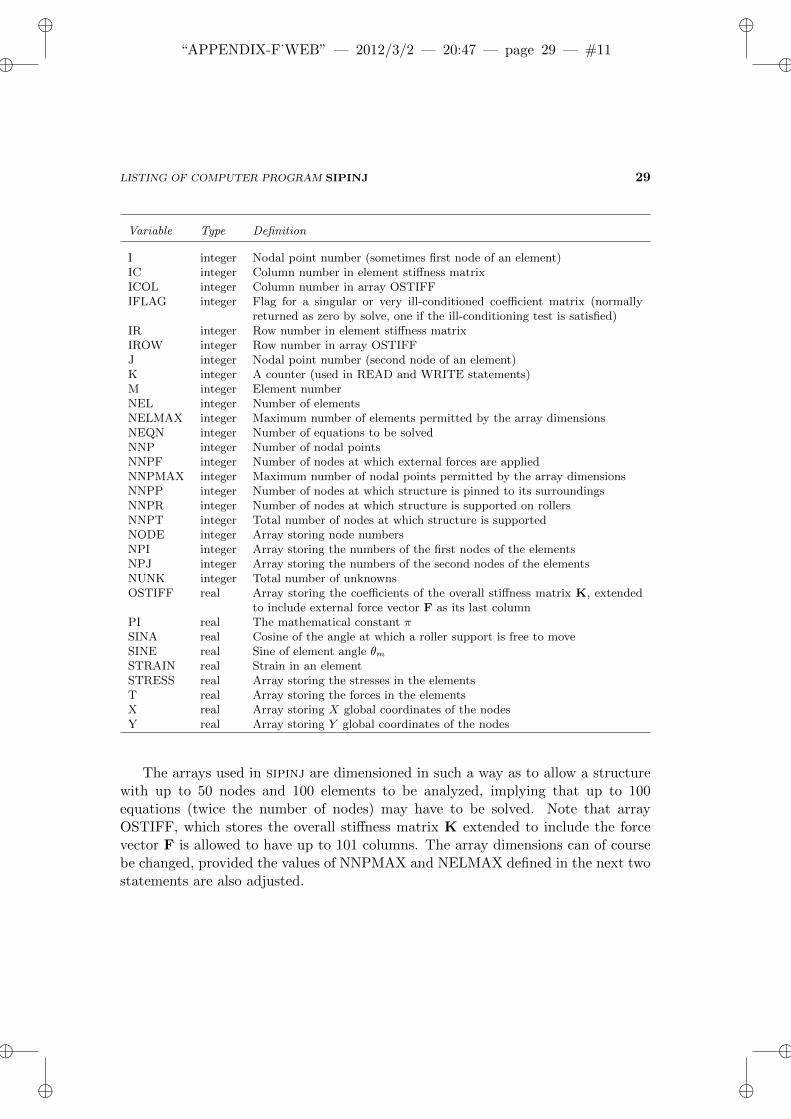
Variable Type Definition
I integer Nodal point number (sometimes first node of an element)IC integer Column number in element stiffness matrixICOL integer Column number in array OSTIFFIFLAG integer Flag for a singular or very ill-conditioned coefficient matrix (normally
returned as zero by solve, one if the ill-conditioning test is satisfied)IR integer Row number in element stiffness matrixIROW integer Row number in array OSTIFFJ integer Nodal point number (second node of an element)K integer A counter (used in READ and WRITE statements)M integer Element numberNEL integer Number of elementsNELMAX integer Maximum number of elements permitted by the array dimensionsNEQN integer Number of equations to be solvedNNP integer Number of nodal pointsNNPF integer Number of nodes at which external forces are appliedNNPMAX integer Maximum number of nodal points permitted by the array dimensionsNNPP integer Number of nodes at which structure is pinned to its surroundingsNNPR integer Number of nodes at which structure is supported on rollersNNPT integer Total number of nodes at which structure is supportedNODE integer Array storing node numbersNPI integer Array storing the numbers of the first nodes of the elementsNPJ integer Array storing the numbers of the second nodes of the elementsNUNK integer Total number of unknownsOSTIFF real Array storing the coefficients of the overall stiffness matrix K, extended
to include external force vector F as its last columnPI real The mathematical constant πSINA real Cosine of the angle at which a roller support is free to moveSINE real Sine of element angle θmSTRAIN real Strain in an elementSTRESS real Array storing the stresses in the elementsT real Array storing the forces in the elementsX real Array storing X global coordinates of the nodesY real Array storing Y global coordinates of the nodes
The arrays used in sipinj are dimensioned in such a way as to allow a structurewith up to 50 nodes and 100 elements to be analyzed, implying that up to 100equations (twice the number of nodes) may have to be solved. Note that arrayOSTIFF, which stores the overall stiffness matrix K extended to include the forcevector F is allowed to have up to 101 columns. The array dimensions can of coursebe changed, provided the values of NNPMAX and NELMAX defined in the next twostatements are also adjusted.
ii
“APPENDIX-F˙WEB” — 2012/3/2 — 20:47 — page 30 — #12 ii
ii
ii
30 LISTINGS OF COMPUTER PROGRAMS
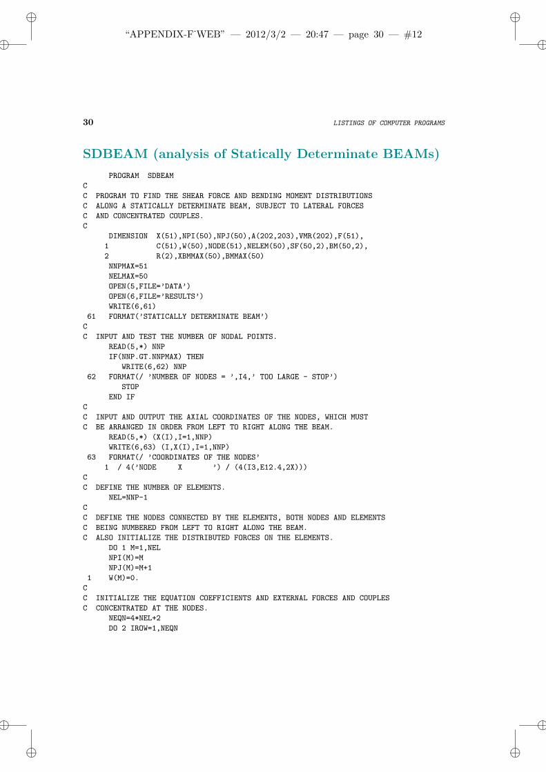
SDBEAM (analysis of Statically Determinate BEAMs)
PROGRAM SDBEAM
C
C PROGRAM TO FIND THE SHEAR FORCE AND BENDING MOMENT DISTRIBUTIONS
C ALONG A STATICALLY DETERMINATE BEAM, SUBJECT TO LATERAL FORCES
C AND CONCENTRATED COUPLES.
C
DIMENSION X(51),NPI(50),NPJ(50),A(202,203),VMR(202),F(51),
1 C(51),W(50),NODE(51),NELEM(50),SF(50,2),BM(50,2),
2 R(2),XBMMAX(50),BMMAX(50)
NNPMAX=51
NELMAX=50
OPEN(5,FILE=’DATA’)
OPEN(6,FILE=’RESULTS’)
WRITE(6,61)
61 FORMAT(’STATICALLY DETERMINATE BEAM’)
C
C INPUT AND TEST THE NUMBER OF NODAL POINTS.
READ(5,*) NNP
IF(NNP.GT.NNPMAX) THEN
WRITE(6,62) NNP
62 FORMAT(/ ’NUMBER OF NODES = ’,I4,’ TOO LARGE - STOP’)
STOP
END IF
C
C INPUT AND OUTPUT THE AXIAL COORDINATES OF THE NODES, WHICH MUST
C BE ARRANGED IN ORDER FROM LEFT TO RIGHT ALONG THE BEAM.
READ(5,*) (X(I),I=1,NNP)
WRITE(6,63) (I,X(I),I=1,NNP)
63 FORMAT(/ ’COORDINATES OF THE NODES’
1 / 4(’NODE X ’) / (4(I3,E12.4,2X)))
C
C DEFINE THE NUMBER OF ELEMENTS.
NEL=NNP-1
C
C DEFINE THE NODES CONNECTED BY THE ELEMENTS, BOTH NODES AND ELEMENTS
C BEING NUMBERED FROM LEFT TO RIGHT ALONG THE BEAM.
C ALSO INITIALIZE THE DISTRIBUTED FORCES ON THE ELEMENTS.
DO 1 M=1,NEL
NPI(M)=M
NPJ(M)=M+1
1 W(M)=0.
C
C INITIALIZE THE EQUATION COEFFICIENTS AND EXTERNAL FORCES AND COUPLES
C CONCENTRATED AT THE NODES.
NEQN=4*NEL+2
DO 2 IROW=1,NEQN
ii
“APPENDIX-F˙WEB” — 2012/3/2 — 20:47 — page 31 — #13 ii
ii
ii
LISTING OF COMPUTER PROGRAM SDBEAM 31
DO 2 ICOL=1,NEQN
2 A(IROW,ICOL)=0.
DO 3 I=1,NNP
F(I)=0.
3 C(I)=0.
C
C INPUT AND TEST THE NUMBER OF NODES AT WHICH EXTERNAL CONCENTRATED
C LATERAL FORCES ARE APPLIED.
READ(5,*) NNPF
IF(NNPF.GT.NNPMAX) THEN
WRITE(6,64) NNPF
64 FORMAT(/ ’NUMBER OF NODES WITH CONCENTRATED FORCES = ’,I4,
1 ’ TOO LARGE - STOP’)
STOP
END IF
C
C INPUT AND OUTPUT THE FORCES AT THESE NODES (DOWNWARDS POSITIVE).
IF(NNPF.GT.0) THEN
READ(5,*) (NODE(K),F(NODE(K)),K=1,NNPF)
WRITE(6,65) (NODE(K),F(NODE(K)),K=1,NNPF)
65 FORMAT(/ ’CONCENTRATED (DOWNWARD) LATERAL FORCES’
1 / ’ NODE’,12X,’F’ / (I5,5X,E15.4))
END IF
C
C INPUT AND TEST THE NUMBER OF NODES AT WHICH EXTERNAL CONCENTRATED
C COUPLES ARE APPLIED.
READ(5,*) NNPC
IF(NNPC.GT.NNPMAX) THEN
WRITE(6,66) NNPC
66 FORMAT(/ ’NUMBER OF NODES WITH CONCENTRATED COUPLES = ’,I4,
1 ’ TOO LARGE - STOP’)
STOP
END IF
C
C INPUT AND OUTPUT THE COUPLES AT THESE NODES (COUNTERCLOCKWISE
C POSITIVE).
IF(NNPC.GT.0) THEN
READ(5,*) (NODE(K),C(NODE(K)),K=1,NNPC)
WRITE(6,67) (NODE(K),C(NODE(K)),K=1,NNPC)
67 FORMAT(/ ’CONCENTRATED (COUNTERCLOCKWISE) COUPLES’
1 / ’ NODE’,12X,’C’ / (I5,5X,E15.4))
END IF
C
C INPUT AND TEST THE NUMBER OF ELEMENTS OVER WHICH EXTERNAL
C DISTRIBUTED LATERAL FORCES ARE APPLIED.
READ(5,*) NELW
IF(NELW.GT.NELMAX) THEN
WRITE(6,68) NELW
ii
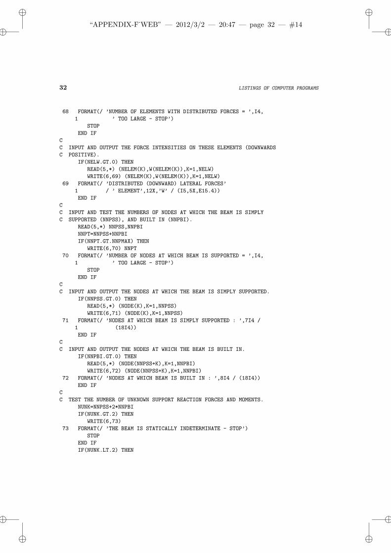
“APPENDIX-F˙WEB” — 2012/3/2 — 20:47 — page 32 — #14 ii
ii
ii
32 LISTINGS OF COMPUTER PROGRAMS
68 FORMAT(/ ’NUMBER OF ELEMENTS WITH DISTRIBUTED FORCES = ’,I4,
1 ’ TOO LARGE - STOP’)
STOP
END IF
C
C INPUT AND OUTPUT THE FORCE INTENSITIES ON THESE ELEMENTS (DOWNWARDS
C POSITIVE).
IF(NELW.GT.0) THEN
READ(5,*) (NELEM(K),W(NELEM(K)),K=1,NELW)
WRITE(6,69) (NELEM(K),W(NELEM(K)),K=1,NELW)
69 FORMAT(/ ’DISTRIBUTED (DOWNWARD) LATERAL FORCES’
1 / ’ ELEMENT’,12X,’W’ / (I5,5X,E15.4))
END IF
C
C INPUT AND TEST THE NUMBERS OF NODES AT WHICH THE BEAM IS SIMPLY
C SUPPORTED (NNPSS), AND BUILT IN (NNPBI).
READ(5,*) NNPSS,NNPBI
NNPT=NNPSS+NNPBI
IF(NNPT.GT.NNPMAX) THEN
WRITE(6,70) NNPT
70 FORMAT(/ ’NUMBER OF NODES AT WHICH BEAM IS SUPPORTED = ’,I4,
1 ’ TOO LARGE - STOP’)
STOP
END IF
C
C INPUT AND OUTPUT THE NODES AT WHICH THE BEAM IS SIMPLY SUPPORTED.
IF(NNPSS.GT.0) THEN
READ(5,*) (NODE(K),K=1,NNPSS)
WRITE(6,71) (NODE(K),K=1,NNPSS)
71 FORMAT(/ ’NODES AT WHICH BEAM IS SIMPLY SUPPORTED : ’,7I4 /
1 (18I4))
END IF
C
C INPUT AND OUTPUT THE NODES AT WHICH THE BEAM IS BUILT IN.
IF(NNPBI.GT.0) THEN
READ(5,*) (NODE(NNPSS+K),K=1,NNPBI)
WRITE(6,72) (NODE(NNPSS+K),K=1,NNPBI)
72 FORMAT(/ ’NODES AT WHICH BEAM IS BUILT IN : ’,8I4 / (18I4))
END IF
C
C TEST THE NUMBER OF UNKNOWN SUPPORT REACTION FORCES AND MOMENTS.
NUNK=NNPSS+2*NNPBI
IF(NUNK.GT.2) THEN
WRITE(6,73)
73 FORMAT(/ ’THE BEAM IS STATICALLY INDETERMINATE - STOP’)
STOP
END IF
IF(NUNK.LT.2) THEN
ii
“APPENDIX-F˙WEB” — 2012/3/2 — 20:47 — page 33 — #15 ii
ii
ii
LISTING OF COMPUTER PROGRAM SDBEAM 33
WRITE(6,74)
74 FORMAT(/ ’THE BEAM IS A MECHANISM - STOP’)
STOP
END IF
C
C SET UP THE LINEAR EQUATIONS, FIRST CONSIDERING EACH ELEMENT IN TURN.
DO 4 M=1,NEL
I=NPI(M)
J=NPJ(M)
ELENGT=X(J)-X(I)
C
C TEST FOR NEGATIVE ELEMENT LENGTH (WHICH RESULTS FROM NODAL
C COORDINATES NOT BEING ENTERED IN ORDER FROM LEFT TO RIGHT ALONG THE
C BEAM.
IF(ELENGT.LT.0.) THEN
WRITE(6,75) M,I,J
75 FORMAT(/ ’ELEMENT ’,I2,’ WITH NODES ’,I2,’ AND ’,I2,
1 ’ HAS NEGATIVE LENGTH - STOP’ /
2 ’(NODAL COORDINATES NOT ENTERED IN ORDER FROM LEFT TO’
3 ’ RIGHT ALONG THE BEAM)’)
STOP
END IF
C
C CONTRIBUTION OF ELEMENT TO FORCE EQUILIBRIUM EQUATION AT ITS FIRST NODE.
A(4*(M-1)+1,4*(M-1)+1)=1.
C
C CONTRIBUTION OF ELEMENT TO MOMENT EQUILIBRIUM EQUATION AT ITS FIRST NODE.
A(4*(M-1)+2,4*(M-1)+2)=-1.
C
C COEFFICIENTS OF EQUATION LINKING SHEAR FORCES AT THE TWO NODES.
A(4*(M-1)+3,4*(M-1)+1)=1.
A(4*(M-1)+3,4*(M-1)+3)=-1.
A(4*(M-1)+3,NEQN+1)=W(M)*ELENGT
C
C COEFFICIENTS OF EQUATION LINKING BENDING MOMENTS AT THE TWO NODES.
A(4*(M-1)+4,4*(M-1)+1)=ELENGT
A(4*(M-1)+4,4*(M-1)+2)=1.
A(4*(M-1)+4,4*(M-1)+4)=-1.
A(4*(M-1)+4,NEQN+1)=0.5*W(M)*ELENGT**2
C
C CONTRIBUTION OF ELEMENT TO FORCE EQUILIBRIUM EQUATION AT ITS SECOND NODE.
A(4*M+1,4*(M-1)+3)=-1.
C
C CONTRIBUTION OF ELEMENT TO MOMENT EQUILIBRIUM EQUATION AT ITS SECOND NODE.
4 A(4*M+2,4*(M-1)+4)=1.
C
C ADD APPLIED CONCENTRATED FORCES AND COUPLES TO THE LINEAR EQUATIONS.
DO 5 I=1,NNP
ii
“APPENDIX-F˙WEB” — 2012/3/2 — 20:47 — page 34 — #16 ii
ii
ii
34 LISTINGS OF COMPUTER PROGRAMS
A(4*(I-1)+1,NEQN+1)=-F(I)
5 A(4*(I-1)+2,NEQN+1)=C(I)
C
C ADD COEFFICIENTS OF UNKNOWN SIMPLE SUPPORT REACTION FORCES TO THE
C LINEAR EQUATIONS.
IF(NNPSS.GT.0) THEN
DO 6 K=1,NNPSS
I=NODE(K)
6 A(4*(I-1)+1,4*NEL+K)=1.
END IF
C
C ADD COEFFICIENTS OF UNKNOWN BUILT-IN SUPPORT REACTION FORCES AND
C MOMENTS TO THE LINEAR EQUATIONS.
IF(NNPBI.GT.0) THEN
DO 7 K=1,NNPBI
I=NODE(K)
A(4*(I-1)+1,4*NEL+NNPSS+2*(K-1)+1)=1.
7 A(4*(I-1)+2,4*NEL+NNPSS+2*(K-1)+2)=-1.
END IF
C
C SOLVE THE LINEAR ALGEBRAIC EQUATIONS BY GAUSSIAN ELIMINATION.
CALL SOLVE(A,VMR,NEQN,4*NELMAX+2,4*NELMAX+3,IFLAG)
C
C STOP IF A UNIT VALUE OF THE ILL-CONDITIONING FLAG IS DETECTED.
IF(IFLAG.EQ.1) THEN
WRITE(6,76)
76 FORMAT(/ ’EQUATIONS ARE ILL-CONDITIONED - STOP’)
STOP
END IF
C
C STORE SHEAR FORCES AND BENDING MOMENTS IN CONVENIENT ARRAYS.
DO 8 M=1,NEL
SF(M,1)=VMR(4*(M-1)+1)
BM(M,1)=VMR(4*(M-1)+2)
SF(M,2)=VMR(4*(M-1)+3)
8 BM(M,2)=VMR(4*(M-1)+4)
C
C ALSO THE REACTION FORCES AND MOMENTS AT THE SUPPORTS.
R(1)=VMR(4*NEL+1)
R(2)=VMR(4*NEL+2)
C
C OUTPUT THE COMPUTED SHEAR FORCES AND BENDING MOMENTS AT THE NODES
C OF EACH ELEMENT.
WRITE(6,77) (M,NPI(M),NPJ(M),SF(M,1),SF(M,2),BM(M,1),BM(M,2),
1 M=1,NEL)
77 FORMAT(/ ’COMPUTED SHEAR FORCES AND BENDING MOMENTS AT THE’
1 ’ NODES OF EACH ELEMENT’ /
2 ’ ELEM NODES SF AT I SF AT J ’
ii
“APPENDIX-F˙WEB” — 2012/3/2 — 20:47 — page 35 — #17 ii
ii
ii
LISTING OF COMPUTER PROGRAM SDBEAM 35
3 ’ BM AT I BM AT J ’ / (3I4,4E15.4))
C
C OUTPUT THE COMPUTED REACTION FORCES AT THE SIMPLE SUPPORTS.
IF(NNPSS.GT.0) THEN
WRITE(6,79) (NODE(K),R(K),K=1,NNPSS)
79 FORMAT(/ ’COMPUTED (DOWNWARD) REACTION FORCES AT THE’
1 ’ SIMPLE SUPPORTS’ / ’ NODE FORCE ’ / (I5,E15.4))
END IF
C
C OUTPUT THE COMPUTED REACTION FORCES AT THE BUILT-IN SUPPORTS.
IF(NNPBI.GT.0) THEN
WRITE(6,80) (NODE(NNPSS+K),R(NNPSS+2*(K-1)+1),K=1,NNPBI)
80 FORMAT(/ ’COMPUTED (DOWNWARD) REACTION FORCES AT THE’
1 ’ BUILT-IN SUPPORTS’ / ’ NODE FORCE ’ / (I5,E15.4))
C
C OUTPUT THE COMPUTED REACTION MOMENTS AT THE BUILT-IN SUPPORTS.
WRITE(6,81) (NODE(NNPSS+K),R(NNPSS+2*(K-1)+2),K=1,NNPBI)
81 FORMAT(/ ’COMPUTED (COUNTERCLOCKWISE) MOMENTS AT THE’
1 ’ BUILT-IN SUPPORTS’ / ’ NODE MOMENT ’ / (I5,E15.4))
END IF
C
C SEARCH FOR MATHEMATICAL MAXIMUM OR MINIMUM VALUES OF BENDING
C MOMENT WITHIN ELEMENTS (WHERE SHEAR FORCE ZERO).
NBMMAX=0
DO 9 M=1,NEL
IF(SF(M,1)*SF(M,2).LE.0.) THEN
NBMMAX=NBMMAX+1
I=NPI(M)
J=NPJ(M)
IF(SF(M,1)*SF(M,2).LT.0.) THEN
XLOCAL=SF(M,1)/W(M)
ELSE
IF(SF(M,1).EQ.0.) XLOCAL=0.
IF(SF(M,2).EQ.0.) XLOCAL=X(J)-X(I)
END IF
XBMMAX(NBMMAX)=X(I)+XLOCAL
BMMAX(NBMMAX)=BM(M,1)+SF(M,1)*XLOCAL-0.5*W(M)*XLOCAL**2
END IF
9 CONTINUE
C
C OUTPUT MATHEMATICAL MAXIMUM OR MINIMUM VALUES OF BENDING MOMENT.
IF(NBMMAX.GT.0) THEN
WRITE(6,82) (XBMMAX(IBMMAX),BMMAX(IBMMAX),IBMMAX=1,NBMMAX)
82 FORMAT(/ ’MATHEMATICAL MAXIMUM OR MINIMUM VALUES OF BENDING’
1 ’ MOMENT’ / ’ AXIAL POSITION MOMENT ’ /
2 (2E15.4))
END IF
C
ii
“APPENDIX-F˙WEB” — 2012/3/2 — 20:47 — page 36 — #18 ii
ii
ii
36 LISTINGS OF COMPUTER PROGRAMS
C FIND GREATEST ABSOLUTE VALUE OF SHEAR FORCE AND GREATEST SAGGING
C AND HOGGING BENDING MOMENTS.
GRSF=0.
XGRSF=0.
GRBMS=0.
XGRBMS=0.
GRBMH=0.
XGRBMH=0.
IF(NBMMAX.GT.0) THEN
DO 10 IBMMAX=1,NBMMAX
IF(BMMAX(IBMMAX).GT.GRBMS) THEN
GRBMS=BMMAX(IBMMAX)
XGRBMS=XBMMAX(IBMMAX)
END IF
IF(BMMAX(IBMMAX).LT.GRBMH) THEN
GRBMH=BMMAX(IBMMAX)
XGRBMH=XBMMAX(IBMMAX)
END IF
10 CONTINUE
END IF
DO 11 M=1,NEL
DO 11 IEND=1,2
IF(IEND.EQ.1) INODE=NPI(M)
IF(IEND.EQ.2) INODE=NPJ(M)
IF(ABS(SF(M,IEND)).GT.GRSF) THEN
GRSF=ABS(SF(M,IEND))
XGRSF=X(INODE)
END IF
IF(BM(M,IEND).GT.GRBMS) THEN
GRBMS=BM(M,IEND)
XGRBMS=X(INODE)
END IF
IF(BM(M,IEND).LT.GRBMH) THEN
GRBMH=BM(M,IEND)
XGRBMH=X(INODE)
END IF
11 CONTINUE
C
C OUTPUT GREATEST ABSOLUTE VALUE OF SHEAR FORCE AND GREATEST SAGGING
C AND HOGGING BENDING MOMENTS, TOGETHER WITH THEIR POSITIONS.
WRITE(6,83) GRSF,XGRSF,GRBMS,XGRBMS,GRBMH,XGRBMH
83 FORMAT(/ ’GREATEST SHEAR FORCE =’,E12.4,’ AT X =’,E12.4
1 /’GREATEST SAGGING BENDING MOMENT =’,E12.4,’ AT X =’,E12.4
2 /’GREATEST HOGGING BENDING MOMENT =’,E12.4,’ AT X =’,E12.4)
STOP
END
ii
“APPENDIX-F˙WEB” — 2012/3/2 — 20:47 — page 37 — #19 ii
ii
ii
LISTING OF COMPUTER PROGRAM SDBEAM 37
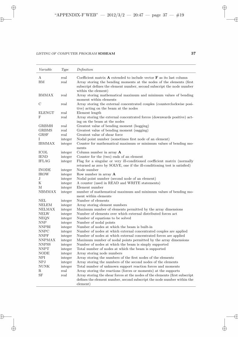
Variable Type Definition
A real Coefficient matrix A extended to include vector F as its last columnBM real Array storing the bending moments at the nodes of the elements (first
subscript defines the element number, second subscript the node numberwithin the element)
BMMAX real Array storing mathematical maximum and minimum values of bendingmoment within elements
C real Array storing the external concentrated couples (counterclockwise posi-tive) acting on the beam at the nodes
ELENGT real Element lengthF real Array storing the external concentrated forces (downwards positive) act-
ing on the beam at the nodesGRBMH real Greatest value of bending moment (hogging)GRBMS real Greatest value of bending moment (sagging)GRSF real Greatest value of shear forceI integer Nodal point number (sometimes first node of an element)IBMMAX integer Counter for mathematical maximum or minimum values of bending mo-
mentsICOL integer Column number in array AIEND integer Counter for the (two) ends of an elementIFLAG integer Flag for a singular or very ill-conditioned coefficient matrix (normally
returned as zero by SOLVE, one if the ill-conditioning test is satisfied)INODE integer Node numberIROW integer Row number in array AJ integer Nodal point number (second node of an element)K integer A counter (used in READ and WRITE statements)M integer Element numberNBMMAX integer number of mathematical maximum and minimum values of bending mo-
ment within elementsNEL integer Number of elementsNELEM integer Array storing element numbersNELMAX integer Maximum number of elements permitted by the array dimensionsNELW integer Number of elements over which external distributed forces actNEQN integer Number of equations to be solvedNNP integer Number of nodal pointsNNPBI integer Number of nodes at which the beam is built-inNNPC integer Number of nodes at which external concentrated couples are appliedNNPF integer Number of nodes at which external concentrated forces are appliedNNPMAX integer Maximum number of nodal points permitted by the array dimensionsNNPSS integer Number of nodes at which the beam is simply supportedNNPT integer Total number of nodes at which the beam is supportedNODE integer Array storing node numbersNPI integer Array storing the numbers of the first nodes of the elementsNPJ integer Array storing the numbers of the second nodes of the elementsNUNK integer Total number of unknown support reaction forces and momentsR real Array storing the reactions (forces or moments) at the supportsSF real Array storing the shear forces at the nodes of the elements (first subscript
defines the element number, second subscript the node number within theelement)
ii
“APPENDIX-F˙WEB” — 2012/3/2 — 20:47 — page 38 — #20 ii
ii
ii
38 LISTINGS OF COMPUTER PROGRAMS
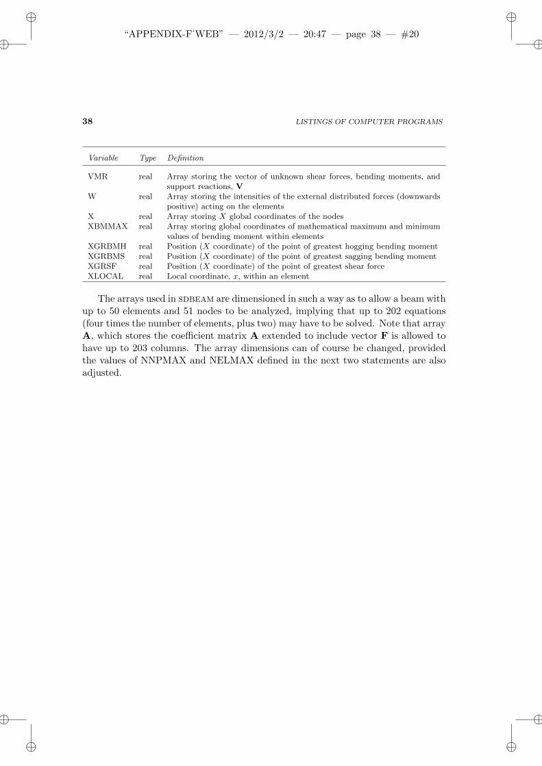
Variable Type Definition
VMR real Array storing the vector of unknown shear forces, bending moments, andsupport reactions, V
W real Array storing the intensities of the external distributed forces (downwardspositive) acting on the elements
X real Array storing X global coordinates of the nodesXBMMAX real Array storing global coordinates of mathematical maximum and minimum
values of bending moment within elementsXGRBMH real Position (X coordinate) of the point of greatest hogging bending momentXGRBMS real Position (X coordinate) of the point of greatest sagging bending momentXGRSF real Position (X coordinate) of the point of greatest shear forceXLOCAL real Local coordinate, x, within an element
The arrays used in sdbeam are dimensioned in such a way as to allow a beam withup to 50 elements and 51 nodes to be analyzed, implying that up to 202 equations(four times the number of elements, plus two) may have to be solved. Note that arrayA, which stores the coefficient matrix A extended to include vector F is allowed tohave up to 203 columns. The array dimensions can of course be changed, providedthe values of NNPMAX and NELMAX defined in the next two statements are alsoadjusted.
ii
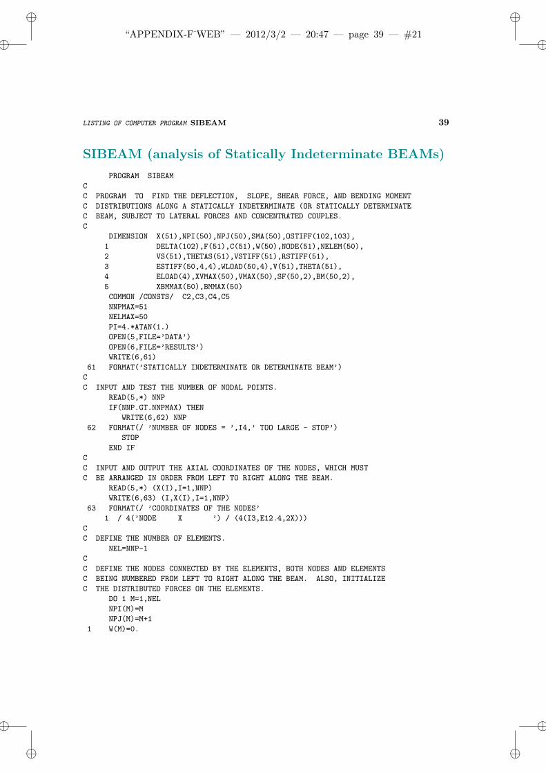
“APPENDIX-F˙WEB” — 2012/3/2 — 20:47 — page 39 — #21 ii
ii
ii
LISTING OF COMPUTER PROGRAM SIBEAM 39
SIBEAM (analysis of Statically Indeterminate BEAMs)
PROGRAM SIBEAM
C
C PROGRAM TO FIND THE DEFLECTION, SLOPE, SHEAR FORCE, AND BENDING MOMENT
C DISTRIBUTIONS ALONG A STATICALLY INDETERMINATE (OR STATICALLY DETERMINATE
C BEAM, SUBJECT TO LATERAL FORCES AND CONCENTRATED COUPLES.
C
DIMENSION X(51),NPI(50),NPJ(50),SMA(50),OSTIFF(102,103),
1 DELTA(102),F(51),C(51),W(50),NODE(51),NELEM(50),
2 VS(51),THETAS(51),VSTIFF(51),RSTIFF(51),
3 ESTIFF(50,4,4),WLOAD(50,4),V(51),THETA(51),
4 ELOAD(4),XVMAX(50),VMAX(50),SF(50,2),BM(50,2),
5 XBMMAX(50),BMMAX(50)
COMMON /CONSTS/ C2,C3,C4,C5
NNPMAX=51
NELMAX=50
PI=4.*ATAN(1.)
OPEN(5,FILE=’DATA’)
OPEN(6,FILE=’RESULTS’)
WRITE(6,61)
61 FORMAT(’STATICALLY INDETERMINATE OR DETERMINATE BEAM’)
C
C INPUT AND TEST THE NUMBER OF NODAL POINTS.
READ(5,*) NNP
IF(NNP.GT.NNPMAX) THEN
WRITE(6,62) NNP
62 FORMAT(/ ’NUMBER OF NODES = ’,I4,’ TOO LARGE - STOP’)
STOP
END IF
C
C INPUT AND OUTPUT THE AXIAL COORDINATES OF THE NODES, WHICH MUST
C BE ARRANGED IN ORDER FROM LEFT TO RIGHT ALONG THE BEAM.
READ(5,*) (X(I),I=1,NNP)
WRITE(6,63) (I,X(I),I=1,NNP)
63 FORMAT(/ ’COORDINATES OF THE NODES’
1 / 4(’NODE X ’) / (4(I3,E12.4,2X)))
C
C DEFINE THE NUMBER OF ELEMENTS.
NEL=NNP-1
C
C DEFINE THE NODES CONNECTED BY THE ELEMENTS, BOTH NODES AND ELEMENTS
C BEING NUMBERED FROM LEFT TO RIGHT ALONG THE BEAM. ALSO, INITIALIZE
C THE DISTRIBUTED FORCES ON THE ELEMENTS.
DO 1 M=1,NEL
NPI(M)=M
NPJ(M)=M+1
1 W(M)=0.
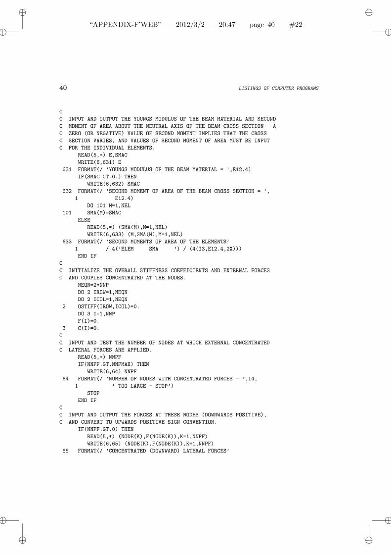
ii
“APPENDIX-F˙WEB” — 2012/3/2 — 20:47 — page 40 — #22 ii
ii
ii
40 LISTINGS OF COMPUTER PROGRAMS
C
C INPUT AND OUTPUT THE YOUNGS MODULUS OF THE BEAM MATERIAL AND SECOND
C MOMENT OF AREA ABOUT THE NEUTRAL AXIS OF THE BEAM CROSS SECTION - A
C ZERO (OR NEGATIVE) VALUE OF SECOND MOMENT IMPLIES THAT THE CROSS
C SECTION VARIES, AND VALUES OF SECOND MOMENT OF AREA MUST BE INPUT
C FOR THE INDIVIDUAL ELEMENTS.
READ(5,*) E,SMAC
WRITE(6,631) E
631 FORMAT(/ ’YOUNGS MODULUS OF THE BEAM MATERIAL = ’,E12.4)
IF(SMAC.GT.0.) THEN
WRITE(6,632) SMAC
632 FORMAT(/ ’SECOND MOMENT OF AREA OF THE BEAM CROSS SECTION = ’,
1 E12.4)
DO 101 M=1,NEL
101 SMA(M)=SMAC
ELSE
READ(5,*) (SMA(M),M=1,NEL)
WRITE(6,633) (M,SMA(M),M=1,NEL)
633 FORMAT(/ ’SECOND MOMENTS OF AREA OF THE ELEMENTS’
1 / 4(’ELEM SMA ’) / (4(I3,E12.4,2X)))
END IF
C
C INITIALIZE THE OVERALL STIFFNESS COEFFICIENTS AND EXTERNAL FORCES
C AND COUPLES CONCENTRATED AT THE NODES.
NEQN=2*NNP
DO 2 IROW=1,NEQN
DO 2 ICOL=1,NEQN
2 OSTIFF(IROW,ICOL)=0.
DO 3 I=1,NNP
F(I)=0.
3 C(I)=0.
C
C INPUT AND TEST THE NUMBER OF NODES AT WHICH EXTERNAL CONCENTRATED
C LATERAL FORCES ARE APPLIED.
READ(5,*) NNPF
IF(NNPF.GT.NNPMAX) THEN
WRITE(6,64) NNPF
64 FORMAT(/ ’NUMBER OF NODES WITH CONCENTRATED FORCES = ’,I4,
1 ’ TOO LARGE - STOP’)
STOP
END IF
C
C INPUT AND OUTPUT THE FORCES AT THESE NODES (DOWNWARDS POSITIVE),
C AND CONVERT TO UPWARDS POSITIVE SIGN CONVENTION.
IF(NNPF.GT.0) THEN
READ(5,*) (NODE(K),F(NODE(K)),K=1,NNPF)
WRITE(6,65) (NODE(K),F(NODE(K)),K=1,NNPF)
65 FORMAT(/ ’CONCENTRATED (DOWNWARD) LATERAL FORCES’
ii
“APPENDIX-F˙WEB” — 2012/3/2 — 20:47 — page 41 — #23 ii
ii
ii
LISTING OF COMPUTER PROGRAM SIBEAM 41
1 / ’ NODE’,12X,’F’ / (I5,5X,E15.4))
DO 31 K=1,NNPF
I=NODE(K)
31 F(I)=-F(I)
END IF
C
C INPUT AND TEST THE NUMBER OF NODES AT WHICH EXTERNAL CONCENTRATED
C COUPLES ARE APPLIED.
READ(5,*) NNPC
IF(NNPC.GT.NNPMAX) THEN
WRITE(6,66) NNPC
66 FORMAT(/ ’NUMBER OF NODES WITH CONCENTRATED COUPLES = ’,I4,
1 ’ TOO LARGE - STOP’)
STOP
END IF
C
C INPUT AND OUTPUT THE COUPLES AT THESE NODES (COUNTERCLOCKWISE
C POSITIVE).
IF(NNPC.GT.0) THEN
READ(5,*) (NODE(K),C(NODE(K)),K=1,NNPC)
WRITE(6,67) (NODE(K),C(NODE(K)),K=1,NNPC)
67 FORMAT(/ ’CONCENTRATED (COUNTERCLOCKWISE) COUPLES’
1 / ’ NODE’,12X,’C’ / (I5,5X,E15.4))
END IF
C
C INPUT AND TEST THE NUMBER OF ELEMENTS OVER WHICH EXTERNAL
C DISTRIBUTED LATERAL FORCES ARE APPLIED.
READ(5,*) NELW
IF(NELW.GT.NELMAX) THEN
WRITE(6,68) NELW
68 FORMAT(/ ’NUMBER OF ELEMENTS WITH DISTRIBUTED FORCES = ’,I4,
1 ’ TOO LARGE - STOP’)
STOP
END IF
C
C INPUT AND OUTPUT THE FORCE INTENSITIES ON THESE ELEMENTS (DOWNWARDS
C POSITIVE).
IF(NELW.GT.0) THEN
READ(5,*) (NELEM(K),W(NELEM(K)),K=1,NELW)
WRITE(6,69) (NELEM(K),W(NELEM(K)),K=1,NELW)
69 FORMAT(/ ’DISTRIBUTED (DOWNWARD) LATERAL FORCES’
1 / ’ ELEMENT’,12X,’W’ / (I5,5X,E15.4))
END IF
C
C INPUT AND TEST THE NUMBERS OF NODES AT WHICH THE BEAM IS SIMPLY
C SUPPORTED (NNPSS), BUILT IN (NNPBI), AND HELD ON FLEXIBLE
C SUPPORTS (NNPFL).
READ(5,*) NNPSS,NNPBI,NNPFL
ii
“APPENDIX-F˙WEB” — 2012/3/2 — 20:47 — page 42 — #24 ii
ii
ii
42 LISTINGS OF COMPUTER PROGRAMS
NNPT=NNPSS+NNPBI+NNPFL
IF(NNPT.GT.NNPMAX) THEN
WRITE(6,70) NNPT
70 FORMAT(/ ’NUMBER OF NODES AT WHICH BEAM IS SUPPORTED = ’,I4,
1 ’ TOO LARGE - STOP’)
STOP
END IF
C
C INPUT AND OUTPUT THE NODES AT WHICH THE BEAM IS SIMPLY SUPPORTED,
C TOGETHER WITH THE DEFLECTIONS (UPWARDS POSITIVE) THERE.
IF(NNPSS.GT.0) THEN
READ(5,*) (NODE(K),VS(NODE(K)),K=1,NNPSS)
WRITE(6,71) (NODE(K),VS(NODE(K)),K=1,NNPSS)
71 FORMAT(/ ’NODES AT WHICH BEAM IS SIMPLY SUPPORTED’ /
1 ’ NODE DEFLECTION’ / (I5,E15.4))
END IF
C
C INPUT AND OUTPUT THE NODES AT WHICH THE BEAM IS BUILT IN, TOGETHER
C WITH THE DEFLECTIONS (UPWARDS POSITIVE) AND SLOPES (IN DEGREES
C MEASURED COUNTERCLOCKWISE FROM THE POSITIVE X-AXIS) THERE.
IF(NNPBI.GT.0) THEN
READ(5,*) (NODE(NNPSS+K),VS(NODE(NNPSS+K)),
1 THETAS(NODE(NNPSS+K)),K=1,NNPBI)
WRITE(6,72) (NODE(NNPSS+K),VS(NODE(NNPSS+K)),
1 THETAS(NODE(NNPSS+K)),K=1,NNPBI)
72 FORMAT(/ ’NODES AT WHICH BEAM IS BUILT IN’ /
1 ’ NODE DEFLECTION SLOPE (DEG)’ / (I5,2E15.4))
END IF
C
C INPUT AND OUTPUT THE NODES AT WHICH THE BEAM IS HELD ON FLEXIBLE
C SUPPORTS, AND THE STIFFNESSES OF THESE SUPPORTS (ROTATIONAL
C STIFFNESSES IN UNITS OF MOMENT PER RADIAN).
IF(NNPFL.GT.0) THEN
READ(5,*) (NODE(NNPSS+NNPBI+K),VSTIFF(NODE(NNPSS+NNPBI+K)),
1 RSTIFF(NODE(NNPSS+NNPBI+K)),K=1,NNPFL)
WRITE(6,721) (NODE(NNPSS+NNPBI+K),VSTIFF(NODE(NNPSS+NNPBI+K)),
1 RSTIFF(NODE(NNPSS+NNPBI+K)),K=1,NNPFL)
721 FORMAT(/ ’NODES AND STIFFNESSES OF THE FLEXIBLE SUPPORTS’ /
1 ’ NODE VERT. STIFF. ROT. STIFF. ’ /
2 (I5,2(5X,E15.4)))
END IF
C
C COUNT THE NUMBER OF NON-ZERO STIFFNESSES OF FLEXIBLE SUPPORTS.
NSTIFF=0
IF(NNPFL.GT.0) THEN
DO 102 K=1,NNPFL
I=NODE(NNPSS+NNPBI+K)
IF(VSTIFF(I).GT.0.) NSTIFF=NSTIFF+1
ii
“APPENDIX-F˙WEB” — 2012/3/2 — 20:47 — page 43 — #25 ii
ii
ii
LISTING OF COMPUTER PROGRAM SIBEAM 43
102 IF(RSTIFF(I).GT.0.) NSTIFF=NSTIFF+1
END IF
C
C TEST THE NUMBER OF UNKNOWN SUPPORT REACTION FORCES AND MOMENTS.
NUNK=NNPSS+2*NNPBI+NSTIFF
IF(NUNK.GT.2) WRITE(6,73)
73 FORMAT(/ ’THE BEAM IS STATICALLY INDETERMINATE’)
IF(NUNK.EQ.2) WRITE(6,731)
731 FORMAT(/ ’THE BEAM IS STATICALLY DETERMINATE’)
IF(NUNK.LT.2) THEN
WRITE(6,74)
74 FORMAT(/ ’THE BEAM IS A MECHANISM - STOP’)
STOP
END IF
C
C SET UP THE LINEAR EQUATIONS, FIRST CONSIDERING EACH ELEMENT IN TURN.
DO 7 M=1,NEL
I=NPI(M)
J=NPJ(M)
ELENGT=X(J)-X(I)
C
C TEST FOR NEGATIVE ELEMENT LENGTH (WHICH RESULTS FROM NODAL COORDINATES
C NOT BEING ENTERED IN ORDER FROM LEFT TO RIGHT ALONG THE BEAM.
IF(ELENGT.LT.0.) THEN
WRITE(6,75) M,I,J
75 FORMAT(/ ’ELEMENT ’,I2,’ WITH NODES ’,I2,’ AND ’,I2,
1 ’ HAS NEGATIVE LENGTH - STOP’ /
2 ’(NODAL COORDINATES NOT ENTERED IN ORDER FROM LEFT TO’
3 ’ RIGHT ALONG THE BEAM)’)
STOP
END IF
C
C COMPUTE THE ELEMENT STIFFNESS MATRIX.
FACT=E*SMA(M)/ELENGT**3
ESTIFF(M,1,1)=FACT*12.
ESTIFF(M,1,2)=FACT*6.*ELENGT
ESTIFF(M,1,3)=-ESTIFF(M,1,1)
ESTIFF(M,1,4)=ESTIFF(M,1,2)
ESTIFF(M,2,1)=ESTIFF(M,1,2)
ESTIFF(M,2,2)=FACT*4.*ELENGT**2
ESTIFF(M,2,3)=-ESTIFF(M,2,1)
ESTIFF(M,2,4)=ESTIFF(M,2,2)/2.
DO 4 IC=1,4
4 ESTIFF(M,3,IC)=-ESTIFF(M,1,IC)
DO 5 IC=1,3
5 ESTIFF(M,4,IC)=ESTIFF(M,IC,4)
ESTIFF(M,4,4)=ESTIFF(M,2,2)
C
ii
“APPENDIX-F˙WEB” — 2012/3/2 — 20:47 — page 44 — #26 ii
ii
ii
44 LISTINGS OF COMPUTER PROGRAMS
C ADD EACH ELEMENT STIFFNESS TO THE OVERALL STIFFNESS MATRIX.
DO 6 IR=1,4
DO 6 IC=1,4
IF(IR.LE.2) IROW=2*(I-1)+IR
IF(IR.GE.3) IROW=2*(J-1)+IR-2
IF(IC.LE.2) ICOL=2*(I-1)+IC
IF(IC.GE.3) ICOL=2*(J-1)+IC-2
6 OSTIFF(IROW,ICOL)=OSTIFF(IROW,ICOL)+ESTIFF(M,IR,IC)
C
C DEFINE THE FORCES AND COUPLES AT THE NODES DUE TO THE
C DISTRIBUTED FORCE ON THE ELEMENT, AND ADD THEM TO THE
C CONCENTRATED FORCES AND COUPLES.
WLOAD(M,1)=-W(M)*ELENGT/2.
WLOAD(M,2)=-W(M)*ELENGT**2/12.
WLOAD(M,3)=WLOAD(M,1)
WLOAD(M,4)=-WLOAD(M,2)
F(I)=F(I)+WLOAD(M,1)
C(I)=C(I)+WLOAD(M,2)
F(J)=F(J)+WLOAD(M,3)
7 C(J)=C(J)+WLOAD(M,4)
C
C STORE THE EXTERNAL FORCES AND COUPLES APPLIED TO THE NODES.
DO 8 I=1,NNP
OSTIFF(2*I-1,NEQN+1)=F(I)
8 OSTIFF(2*I,NEQN+1)=C(I)
C
C IMPOSE THE GIVEN DEFLECTIONS AT THE SIMPLE SUPPORTS.
IF(NNPSS.GT.0) THEN
DO 10 K=1,NNPSS
I=NODE(K)
DO 9 J=1,NEQN
9 OSTIFF(2*I-1,J)=0.
OSTIFF(2*I-1,2*I-1)=1.
10 OSTIFF(2*I-1,NEQN+1)=VS(I)
END IF
C
C IMPOSE THE GIVEN DEFLECTIONS AND SLOPES AT THE BUILT-IN SUPPORTS,
C CONVERTING SLOPES FROM DEGREES TO RADIANS.
IF(NNPBI.GT.0) THEN
DO 12 K=1,NNPBI
I=NODE(NNPSS+K)
DO 11 J=1,NEQN
OSTIFF(2*I-1,J)=0.
11 OSTIFF(2*I,J)=0.
OSTIFF(2*I-1,2*I-1)=1.
OSTIFF(2*I,2*I)=1.
OSTIFF(2*I-1,NEQN+1)=VS(I)
12 OSTIFF(2*I,NEQN+1)=THETAS(I)*PI/180.
ii
“APPENDIX-F˙WEB” — 2012/3/2 — 20:47 — page 45 — #27 ii
ii
ii
LISTING OF COMPUTER PROGRAM SIBEAM 45
END IF
C
C IMPOSE THE STIFFNESS RELATIONSHIPS AT THE FLEXIBLE SUPPORTS.
IF(NNPFL.GT.0) THEN
DO 13 K=1,NNPFL
I=NODE(NNPSS+NNPBI+K)
OSTIFF(2*I-1,2*I-1)=OSTIFF(2*I-1,2*I-1)+VSTIFF(I)
13 OSTIFF(2*I,2*I)=OSTIFF(2*I,2*I)+RSTIFF(I)
END IF
C
C SOLVE THE LINEAR ALGEBRAIC EQUATIONS BY GAUSSIAN ELIMINATION.
CALL SOLVE(OSTIFF,DELTA,NEQN,2*NNPMAX,2*NNPMAX+1,IFLAG)
C
C STOP IF A UNIT VALUE OF THE ILL-CONDITIONING FLAG IS DETECTED.
IF(IFLAG.EQ.1) THEN
WRITE(6,76)
76 FORMAT(/ ’EQUATIONS ARE ILL-CONDITIONED - STOP’)
STOP
END IF
C
C STORE DEFLECTIONS AND SLOPES IN CONVENIENT ARRAYS.
DO 14 I=1,NNP
V(I)=DELTA(2*I-1)
14 THETA(I)=DELTA(2*I)
C
C OUTPUT THE COMPUTED DEFLECTIONS AND SLOPES AT THE NODAL POINTS.
WRITE(6,761) (I,V(I),THETA(I),I=1,NNP)
761 FORMAT(/ ’COMPUTED DEFLECTIONS AND SLOPES AT THE NODES’ /
1 2(’ NODE V SLOPE ’) / 2(I4,2E15.4,2X))
C
C SEARCH FOR MATHEMATICAL MAXIMUM OR MINIMUM VALUES OF DEFLECTION
C WITHIN ELEMENTS (WHERE SLOPE ZERO).
NVMAX=0
DO 15 M=1,NEL
I=NPI(M)
J=NPJ(M)
ELENGT=X(J)-X(I)
C1=V(I)
C2=THETA(I)
C3=-3.*V(I)/ELENGT**2-2.*THETA(I)/ELENGT+3.*V(J)/ELENGT**2
1 -THETA(J)/ELENGT-W(M)*ELENGT**2/(24.*E*SMA(M))
C4=2.*V(I)/ELENGT**3+THETA(I)/ELENGT**2-2.*V(J)/ELENGT**3
1 +THETA(J)/ELENGT**2+W(M)*ELENGT/(12.*E*SMA(M))
C5=-W(M)/(24.*E*SMA(M))
C
C SUBDIVIDE THE ELEMENT INTO 100 STEPS FOR SEARCH PURPOSES.
DO 15 ISTEP=1,100
X1=0.01*ELENGT*REAL(ISTEP-1)
ii
“APPENDIX-F˙WEB” — 2012/3/2 — 20:47 — page 46 — #28 ii
ii
ii
46 LISTINGS OF COMPUTER PROGRAMS
X2=X1+0.01*ELENGT
THETA1=C2+2.*C3*X1+3.*C4*X1**2+4.*C5*X1**3
THETA2=C2+2.*C3*X2+3.*C4*X2**2+4.*C5*X2**3
IF(THETA1*THETA2.LE.0.) THEN
NVMAX=NVMAX+1
CALL BISECT(X1,X2,1.0E-6*ELENGT,XLOCAL,IFLAG)
XVMAX(NVMAX)=X(I)+XLOCAL
VMAX(NVMAX)=C1+C2*XLOCAL+C3*XLOCAL**2+C4*XLOCAL**3+C5*XLOCAL**4
END IF
15 CONTINUE
C
C OUTPUT MATHEMATICAL MAXIMUM OR MINIMUM VALUES OF DEFLECTION.
IF(NVMAX.GT.0) THEN
WRITE(6,762) (XVMAX(IVMAX),VMAX(IVMAX),IVMAX=1,NVMAX)
762 FORMAT(/ ’MATHEMATICAL MAXIMUM OR MINIMUM VALUES OF DEFLECTION’
1 / ’ AXIAL POSITION DEFLECTION ’ /
2 (2E15.4))
END IF
C
C FIND GREATEST VALUE OF DEFLECTION.
GRVP=0.
XGRVP=0.
GRVN=0.
XGRVN=0.
IF(NVMAX.GT.0) THEN
DO 16 IVMAX=1,NVMAX
IF(VMAX(IVMAX).GT.GRVP) THEN
GRVP=VMAX(IVMAX)
XGRVP=XVMAX(IVMAX)
END IF
IF(VMAX(IVMAX).LT.GRVN) THEN
GRVN=VMAX(IVMAX)
XGRVN=XVMAX(IVMAX)
END IF
16 CONTINUE
END IF
DO 17 M=1,NEL
DO 17 IEND=1,2
IF(IEND.EQ.1) INODE=NPI(M)
IF(IEND.EQ.2) INODE=NPJ(M)
IF(V(INODE).GT.GRVP) THEN
GRVP=V(INODE)
XGRVP=X(INODE)
END IF
IF(V(INODE).LT.GRVN) THEN
GRVN=V(INODE)
XGRVN=X(INODE)
END IF
ii
“APPENDIX-F˙WEB” — 2012/3/2 — 20:47 — page 47 — #29 ii
ii
ii
LISTING OF COMPUTER PROGRAM SIBEAM 47
17 CONTINUE
C
C OUTPUT THE GREATEST VALUES OF DEFLECTION.
WRITE(6,763) GRVP,XGRVP,GRVN,XGRVN
763 FORMAT(
1 /’GREATEST UPWARD DEFLECTION =’,E12.4,’ AT X =’,E12.4
2 /’GREATEST DOWNWARD DEFLECTION =’,E12.4,’ AT X =’,E12.4)
C
C COMPUTE SHEAR FORCES AND BENDING MOMENTS.
DO 19 M=1,NEL
I=NPI(M)
J=NPJ(M)
DO 18 IR=1,4
18 ELOAD(IR)=ESTIFF(M,IR,1)*V(I)+ESTIFF(M,IR,2)*THETA(I)
1 +ESTIFF(M,IR,3)*V(J)+ESTIFF(M,IR,4)*THETA(J)-WLOAD(M,IR)
SF(M,1)=ELOAD(1)
BM(M,1)=-ELOAD(2)
SF(M,2)=-ELOAD(3)
19 BM(M,2)=ELOAD(4)
C
C OUTPUT THE COMPUTED SHEAR FORCES AND BENDING MOMENTS AT THE NODES
C OF EACH ELEMENT.
WRITE(6,77) (M,NPI(M),NPJ(M),SF(M,1),SF(M,2),BM(M,1),BM(M,2),
1 M=1,NEL)
77 FORMAT(/ ’COMPUTED SHEAR FORCES AND BENDING MOMENTS AT THE’
1 ’ NODES OF EACH ELEMENT’ /
2 ’ ELEM NODES SF AT I SF AT J ’
3 ’ BM AT I BM AT J ’ / (3I4,4E15.4))
C
C SEARCH FOR MATHEMATICAL MAXIMUM OR MINIMUM VALUES OF BENDING
C MOMENT WITHIN ELEMENTS (WHERE SHEAR FORCE ZERO).
NBMMAX=0
DO 20 M=1,NEL
IF(SF(M,1)*SF(M,2).LE.0.) THEN
NBMMAX=NBMMAX+1
I=NPI(M)
J=NPJ(M)
IF(SF(M,1)*SF(M,2).LT.0.) THEN
XLOCAL=SF(M,1)/W(M)
ELSE
IF(SF(M,1).EQ.0.) XLOCAL=0.
IF(SF(M,2).EQ.0.) XLOCAL=X(J)-X(I)
END IF
XBMMAX(NBMMAX)=X(I)+XLOCAL
BMMAX(NBMMAX)=BM(M,1)+SF(M,1)*XLOCAL-0.5*W(M)*XLOCAL**2
END IF
20 CONTINUE
C
ii
“APPENDIX-F˙WEB” — 2012/3/2 — 20:47 — page 48 — #30 ii
ii
ii
48 LISTINGS OF COMPUTER PROGRAMS
C OUTPUT MATHEMATICAL MAXIMUM OR MINIMUM VALUES OF BENDING MOMENT.
IF(NBMMAX.GT.0) THEN
WRITE(6,82) (XBMMAX(IBMMAX),BMMAX(IBMMAX),IBMMAX=1,NBMMAX)
82 FORMAT(/ ’MATHEMATICAL MAXIMUM OR MINIMUM VALUES OF BENDING’
1 ’ MOMENT’ / ’ AXIAL POSITION MOMENT ’ /
2 (2E15.4))
END IF
C
C FIND GREATEST VALUES OF SHEAR FORCE AND BENDING MOMENT.
GRSF=0.
XGRSF=0.
GRBMS=0.
XGRBMS=0.
GRBMH=0.
XGRBMH=0.
IF(NBMMAX.GT.0) THEN
DO 21 IBMMAX=1,NBMMAX
IF(BMMAX(IBMMAX).GT.GRBMS) THEN
GRBMS=BMMAX(IBMMAX)
XGRBMS=XBMMAX(IBMMAX)
END IF
IF(BMMAX(IBMMAX).LT.GRBMH) THEN
GRBMH=BMMAX(IBMMAX)
XGRBMH=XBMMAX(IBMMAX)
END IF
21 CONTINUE
END IF
DO 22 M=1,NEL
DO 22 IEND=1,2
IF(IEND.EQ.1) INODE=NPI(M)
IF(IEND.EQ.2) INODE=NPJ(M)
IF(ABS(SF(M,IEND)).GT.GRSF) THEN
GRSF=ABS(SF(M,IEND))
XGRSF=X(INODE)
END IF
IF(BM(M,IEND).GT.GRBMS) THEN
GRBMS=BM(M,IEND)
XGRBMS=X(INODE)
END IF
IF(BM(M,IEND).LT.GRBMH) THEN
GRBMH=BM(M,IEND)
XGRBMH=X(INODE)
END IF
22 CONTINUE
C
C OUTPUT THE GREATEST VALUES OF SHEAR FORCE AND BENDING MOMENT.
WRITE(6,83) GRSF,XGRSF,GRBMS,XGRBMS,GRBMH,XGRBMH
83 FORMAT(/ ’GREATEST SHEAR FORCE =’,E12.4,’ AT X =’,E12.4
ii
“APPENDIX-F˙WEB” — 2012/3/2 — 20:47 — page 49 — #31 ii
ii
ii
LISTING OF COMPUTER PROGRAM SIBEAM 49
1 /’GREATEST SAGGING BENDING MOMENT =’,E12.4,’ AT X =’,E12.4
2 /’GREATEST HOGGING BENDING MOMENT =’,E12.4,’ AT X =’,E12.4)
STOP
END
FUNCTION FN(X,IOTEST)
C
C FUNCTION SUBPROGRAM TO DEFINE THE CUBIC FUNCTION FOR SLOPE WITHIN
C AN ELEMENT.
COMMON /CONSTS/ C2,C3,C4,C5
FN=C2+2.*C3*X+3.*C4*X**2+4.*C5*X**3
RETURN
END
Variable Type Definition
BM real Array storing the bending moments at the nodes of the elements (firstsubscript defines the element number, second subscript the node numberwithin the element)
BMMAX real Array storing mathematical maximum and minimum values of bendingmoment within elements
C real Array storing the external concentrated couples (counterclockwise posi-tive) acting on the beam at the nodes
C1 to C5 real Shape function constants C1 to C5
DELTA real Array storing the deflections and slopes at the nodal pointsE real Young’s modulus of the beam materialELENGT real Element lengthELOAD real Array storing components of the element load vector fmESTIFF real Array storing the stiffness coefficients for all the elements (first subscript
defines the element number, second and third subscripts the row and col-umn numbers of the element stiffness matrix)
F real Array storing the external concentrated forces (downward positive) actingon the beam at the nodes
FACT real Common factor in the element stiffness coefficientsGRBMH real Greatest value of bending moment (hogging)GRBMS real Greatest value of bending moment (sagging)GRSF real Greatest value of shear forceGRVP real Greatest value of deflection (positive)GRVN real Greatest value of deflection (negative)I integer Nodal point number (sometimes first node of an element)IBMMAX integer Counter for mathematical maximum or minimum values of bending mo-
mentsIC integer Column number in array ESTIFFICOL integer Column number in array OSTIFF
ii
“APPENDIX-F˙WEB” — 2012/3/2 — 20:47 — page 50 — #32 ii
ii
ii
50 LISTINGS OF COMPUTER PROGRAMS
Variable Type Definition
IEND integer Counter for the (two) ends of an elementIFLAG integer Flag for a singular or very ill-conditioned coefficient matrix (normally
returned as zero by SOLVE, one if the ill-conditioning test is satisfied)INODE integer Node numberIR integer Row number in array ESTIFFIROW integer Row number in array OSTIFFISTEP integer Counter for steps along an element when searching for maximum or min-
imum deflectionsIVMAX integer Counter for mathematical maximum or minimum values of deflectionJ integer Nodal point number (second node of an element)K integer A counter (used in READ and WRITE statements)M integer Element numberNBMMAX integer Number of mathematical maximum and minimum values of bending mo-
ment within elementsNEL integer Number of elementsNELEM integer Array storing element numbersNELMAX integer Maximum number of elements permitted by the array dimensionsNELW integer Number of elements over which external distributed forces actNEQN integer Number of equations to be solvedNNP integer Number of nodal pointsNNPC integer Number of nodes at which external concentrated couples are appliedNNPF integer Number of nodes at which external concentrated forces are appliedNNPMAX integer Maximum number of nodal points permitted by the array dimensionsNNPBI integer Number of nodes at which the beam is built inNNPFL integer Number of nodes at which the beam is supported on flexible supportsNNPSS integer Number of nodes at which the beam is simply supportedNNPT integer Total number of nodes at which the beam is supportedNODE integer Array storing node numbersNPI integer Array storing the numbers of the first nodes of the elementsNPJ integer Array storing the numbers of the second nodes of the elementsNSTIFF integer Number of non-zero stiffnesses of flexible supportsNUNK integer Total number of unknown support reaction forces and momentsNVMAX integer Number of mathematical maximum and minimum values of deflection
within elementsOSTIFF real Array storing coefficients of the overall stiffness matrix K, extended to
include external force vector F∗ as its last columnPI real The mathematical constant πRSTIFF real Array storing the rotational stiffnesses of the flexible supports (in units
of moment per radian)SF real Array storing the shear forces at the nodes of the elements (first subscript
defines the. element number, second subscript the node number withinthe element)
SMA real Array storing the second moments of area of the elementsSMAC real Constant second moment of area for a uniform beam
ii
“APPENDIX-F˙WEB” — 2012/3/2 — 20:47 — page 51 — #33 ii
ii
ii
LISTING OF COMPUTER PROGRAM SIBEAM 51
Variable Type Definition
THETA real Array storing the slopes (in radians) at the nodal pointsTHETAS real Array storing the slopes (in degrees) at the support pointsTHETA1 real Slope at the beginning of a step within an elementTHETA2 real Slope at the end of a step within an elementV real Array storing the deflections at the nodal pointsVMAX real Array storing mathematical maximum and minimum values of deflection
within elementsVS real Array storing the deflections at the support pointsVSTIFF real Array storing the vertical stiffnesses of the flexible supportsW real Array storing the intensities of the external distributed forces (downward
positive) acting on the elementsWLOAD real Array storing the external load terms Wm associated with the distributed
lateral forces, for all the elements (first subscript defines the element num-ber, second subscript the row number)
X real Array storing X global coordinates of the nodesX1 real Local coordinate at the beginning of a step within an elementX2 real Local coordinate at the end of a step within an elementXBMMAX real Array storing global coordinates of mathematical maximum and minimum
values of bending moment within elementsXGRBMH real Position (X coordinate) of the point of greatest hogging bending momentXGRBMS real Position (X coordinate) of the point of greatest sagging bending momentXGRSF real Position (X coordinate) of the point of greatest shear forceXGRVN real Position (X coordinate) of the point of greatest negative deflectionXGRVP real Position (X coordinate) of the point of greatest positive deflectionXLOCAL real Local coordinate, x, within an elementXVMAX real Array storing global coordinates of mathematical maximum and minimum
values of deflection within elements
The arrays used in sibeam are dimensioned in such a way as to allow a beam with upto 50 elements and 51 nodes to be analyzed, implying that up to 102 equations (twicethe number of nodes) may have to be solved. Note that array OSTIFF, which storesthe overall stiffness matrix K extended to include vector F∗ is allowed to have up to103 columns. The array dimensions can of course be changed, provided the valuesof NNPMAX and NELMAX defined in the next two statements are also adjusted.
ii
“APPENDIX-F˙WEB” — 2012/3/2 — 20:47 — page 52 — #34 ii
ii
ii
52 LISTINGS OF COMPUTER PROGRAMS
ROSETTE (determination of states of strain and stressfrom strain ROSETTE)
PROGRAM ROSETTE
C
C PROGRAM TO DETERMINE THE STATE OF STRAIN AND STRESS FROM
C STRAIN ROSETTE MEASUREMENTS.
C
DIMENSION EN(3),A(3,4),EXY(3),THETA(3),SIGXY(3),EP(2),
1 SIGP(2),THETAP(2)
REAL NU
OPEN(5,FILE=’DATA’)
OPEN(6,FILE=’RESULTS’)
PI=4.*ATAN(1.)
WRITE(6,61)
61 FORMAT(’STRESSES AND STRAINS DERIVED FROM STRAIN ROSETTE’
1 ’ MEASUREMENTS’)
C
C INPUT THE YOUNGS MODULUS AND POISSONS RATIO OF THE MATERIAL.
READ(5,*) E,NU
WRITE(6,62) E,NU
62 FORMAT(/ ’YOUNGS MODULUS = ’,E12.4,10X,’POISSONS RATIO = ’,F5.3)
C
C INPUT THE ANGULAR ORIENTATIONS (IN DEGREES) OF THE THREE STRAIN
C GAGES, MEASURED COUNTERCLOCKWISE FROM SOME REFERENCE DIRECTION
C (WHICH WILL BE TREATED AS THE X AXIS).
READ(5,*) (THETA(I),I=1,3)
C
C INPUT IN THE SAME ORDER THE NORMAL STRAINS MEASURED BY THESE GAGES.
READ(5,*) (EN(I),I=1,3)
C
C OUTPUT THE GAGE ORIENTATIONS AND MEASURED STRAINS.
WRITE(6,63) (I,THETA(I),EN(I),I=1,3)
63 FORMAT(/ ’ANGULAR ORIENTATIONS OF THE GAGES IN DEGREES MEASURED’
1 / ’COUNTERCLOCKWISE FROM THE X AXIS, AND THE MEASURED STRAINS’
2 / ’ GAGE NO. THETA EN’ / (I8,F14.2,E15.4))
C
C SET UP THE LINEAR EQUATIONS.
DO 1 I=1,3
ANG=THETA(I)*PI/180.
SINT=SIN(ANG)
COST=COS(ANG)
A(I,1)=COST**2
A(I,2)=SINT**2
A(I,3)=SINT*COST
1 A(I,4)=EN(I)
C
ii
“APPENDIX-F˙WEB” — 2012/3/2 — 20:47 — page 53 — #35 ii
ii
ii
LISTING OF COMPUTER PROGRAM ROSETTE 53
C SOLVE THE EQUATIONS.
CALL SOLVE(A,EXY,3,3,4,IFLAG)
C
C A UNIT VALUE OF THE ILL-CONDITIONING FLAG IMPLIES DATA ERROR OR
C GAGES UNSUITABLY ARRANGED.
IF(IFLAG.EQ.1) THEN
WRITE(6,64)
64 FORMAT(/ ’DATA ERROR OR GAGES UNSUITABLY ARRANGED - STOP’)
STOP
END IF
C
C OUTPUT THE IN-PLANE STRAINS IN THE (X,Y) COORDINATE SYSTEM.
WRITE(6,65) (EXY(I),I=1,3)
65 FORMAT(/’COMPUTED IN-PLANE STRAINS IN THE (X,Y) COORDINATE SYSTEM’
1 / ’EX = ’,E12.4,5X,’EY = ’,E12.4,5X,’GAMXY = ’,E12.4)
C
C CALCULATE AND OUTPUT THE CORRESPONDING IN-PLANE STRESSES.
DENOM=1.-NU**2
SIGXY(1)=E*(EXY(1)+NU*EXY(2))/DENOM
SIGXY(2)=E*(EXY(2)+NU*EXY(1))/DENOM
G=0.5*E/(1.+NU)
SIGXY(3)=G*EXY(3)
WRITE(6,66) (SIGXY(I),I=1,3)
66 FORMAT(/ ’COMPUTED STRESSES IN THE (X,Y) COORDINATE SYSTEM’
1 / ’SIGX = ’,E12.4,5X,’SIGY = ’,E12.4,5X,’TAUXY = ’,E12.4)
C
C ANALYZE THE STATE OF STRESS AND STRAIN AT THE POINT CONCERNED.
CALL POINT(’STRAIN’,EXY,THETAP,EP,ESMAX,AESMAX,SE)
CALL POINT(’STRESS’,SIGXY,THETAP,SIGP,SSMAX,ASSMAX,SE)
C
C CALCULATE THE THIRD PRINCIPAL STRAIN (WHICH IS NOT ZERO), AND
C CORRECT THE ABSOLUTE MAXIMUM SHEAR STRAIN.
EP3=-NU*(SIGP(1)+SIGP(2))/E
AESMAX=MAX(EP(1)-EP(2),ABS(EP(2)-EP3),ABS(EP3-EP(1)))
C
C OUTPUT THE PRINCIPAL STRESSES AND STRAINS AND THE DIRECTIONS OF THE
C NORMALS TO THE CORRESPONDING PRINCIPAL PLANES.
WRITE(6,67) (I,SIGP(I),EP(I),THETAP(I),I=1,2)
67 FORMAT(/ ’PRINCIPAL STRESSES AND STRAINS, AND DIRECTIONS OF THE’
1 ’ PRINCIPAL PLANES’
2 / ’(IN DEGREES MEASURED COUNTERCLOCKWISE FROM THE X AXIS)’
3 / ’ NO. STRESS STRAIN DIRECTION’
4 / (I3,2E15.4,5X,F8.1))
WRITE(6,68) EP3
68 FORMAT(’ (3’,’ 0. ’,E15.4,’ OUT OF PLANE)’)
C
C OUTPUT THE MAXIMUM SHEAR STRESSES AND STRAINS.
WRITE(6,69) SSMAX,ESMAX,ASSMAX,AESMAX
ii
“APPENDIX-F˙WEB” — 2012/3/2 — 20:47 — page 54 — #36 ii
ii
ii
54 LISTINGS OF COMPUTER PROGRAMS
69 FORMAT(/ ’MAXIMUM SHEAR STRESSES AND STRAINS’
1 / 32X,’ STRESS STRAIN’
2 / ’MAXIMUM IN-PLANE SHEAR VALUES = ’,2E15.4
3 / ’ABSOLUTE MAXIMUM SHEAR VALUES = ’,2E15.4)
C
C OUTPUT THE VON MISES EQUIVALENT STRESS.
WRITE(6,70) SE
70 FORMAT(/ ’VON MISES EQUIVALENT STRESS = ’,E12.4)
STOP
END
The following list provides the definitions of the fortran variables used.
Variable Type Definition
A real Array storing the coefficients of linear equations in Equation (9.43)AESMAX real Absolute maximum shear strainANG real Angle θ of gage orientation in radiansASSMAX real Absolute maximum shear stressCOST real Cosine of angle θ of gage orientationDENOM real Denominator expression (1 − ν2) in Equation (9.45)E real Young’s modulusEN real Array storing the normal strains measured by the three gagesEP real Array storing the two in-plane principal strainsEP3 real Third (out of plane) principal strainESMAX real Maximum in-plane shear strainEXY real Array storing the strains ex, ey and γxyG real Shear modulusI integer A counterIFLAG integer Flag for a singular or very ill-conditioned coefficient matrix (normally
returned as zero by SOLVE, one if the ill-conditioning test is satisfied)NU real Poisson’s ratioPI real The mathematical constant πSE real Von Mises equivalent stressSIGP real Array storing the two in-plane principal stressesSIGXY real Array storing the stresses σx, σy and τxySINT real Sine of angle θ of gage orientationSSMAX real Maximum in-plane shear stressTHETA real Array storing the angular orientations (in degrees) of the three gagesTHETAP real Array storing the directions of the normals to the principal planes
ii
“APPENDIX-F˙WEB” — 2012/3/2 — 20:47 — page 55 — #37 ii
ii
ii
LISTING OF COMPUTER PROGRAM ANAL2D 55
ANAL2D (ANALysis of 2D states of stress or strain at apoint)
PROGRAM ANAL2D
C
C PROGRAM TO ANALYZE A TWO-DIMENSIONAL STATE OF STRESS OR STRAIN
C AT A POINT.
C
DIMENSION SXY(3),S(2),THETAP(2)
CHARACTER*6 CASE
OPEN(5,FILE=’DATA’)
OPEN(6,FILE=’RESULTS’)
C
C INPUT 6 CHARACTER WORD ’STRESS’ OR ’STRAIN’ TO INDICATE THE TYPE
C OF CASE TO BE TREATED.
READ(5,*) CASE
WRITE(6,61) CASE
61 FORMAT(’ANALYSIS OF A TWO-DIMENSIONAL STATE OF ’,A6,’ AT A POINT’)
C
C INPUT THE STRESSES/STRAINS IN THE (X,Y) COORDINATE SYSTEM,IN THE
C ORDER OF X COMPONENT, Y COMPONENT, AND XY (SHEAR) COMPONENT.
READ(5,*) (SXY(I),I=1,3)
WRITE(6,62) (SXY(I),I=1,3)
62 FORMAT(/ ’COMPONENTS IN THE (X,Y) COORDINATE SYSTEM’/
1 ’SX = ’,E12.4,5X,’SY = ’,E12.4,5X,’SXY = ’,E12.4)
C
C CARRY OUT THE ANALYSIS.
CALL POINT(CASE,SXY,THETAP,S,SHMAX,ASHMAX,SE)
C
C OUTPUT THE PRINCIPAL VALUES AND THE DIRECTIONS OF THE NORMALS TO THE
C CORRESPONDING PRINCIPAL PLANES.
WRITE(6,63) (I,S(I),THETAP(I),I=1,2)
63 FORMAT(/ ’PRINCIPAL VALUES AND DIRECTIONS OF THE PRINCIPAL PLANES’
1 / ’(IN DEGREES MEASURED COUNTERCLOCKWISE FROM THE X AXIS)’
2 / ’ NO. VALUE DIRECTION’
3 / (I3,E15.4,F8.1))
C
C OUTPUT THE MAXIMUM SHEAR VALUES.
WRITE(6,64) SHMAX,ASHMAX
64 FORMAT(/ ’MAXIMUM IN-PLANE SHEAR VALUE = ’,E12.4
1 / ’ABSOLUTE MAXIMUM SHEAR VALUE = ’,E12.4)
C
C FOR A CASE OF PLANE STRESS, OUTPUT THE VON MISES EQUIVALENT STRESS.
IF(CASE.EQ.’STRESS’) WRITE(6,65) SE
65 FORMAT(/ ’VON MISES EQUIVALENT STRESS = ’,E12.4)
STOP
END
ii
“APPENDIX-F˙WEB” — 2012/3/2 — 20:47 — page 56 — #38 ii
ii
ii
56 LISTINGS OF COMPUTER PROGRAMS
SUBROUTINE POINT(CASE,SXY,THETAP,S,SHMAX,ASHMAX,SE)
C
C SUBROUTINE TO ANALYZE THE STATE OF TWO-DIMENSIONAL STRESS OR
C STRAIN AT A POINT, GIVEN TWO NORMAL COMPONENTS AND ONE SHEAR
C COMPONENT IN A PARTICULAR ORTHOGONAL COORDINATE SYSTEM - HERE
C LABELLED X AND Y.
C
DIMENSION SXY(3),S(2),THETAP(2)
CHARACTER*6 CASE
PI=4.*ATAN(1.)
C
C IF THE CASE IS ONE OF TWO-DIMENSIONAL STRAIN, THE SHEAR TERM IS
C HALVED.
IF(CASE.EQ.’STRAIN’) SXY(3)=0.5*SXY(3)
C
C FIND THE ANGLES OF THE NORMALS TO THE PRINCIPAL PLANES.
TWOPHI=ATAN2(2.*SXY(3),SXY(1)-SXY(2))
IF(TWOPHI.LT.0.) TWOPHI=TWOPHI+PI
THETAP(1)=0.5*TWOPHI
THETAP(2)=THETAP(1)+0.5*PI
C
C FIND THE PRINCIPAL STRESSES/STRAINS.
DO 1 I=1,2
1 S(I)=0.5*(SXY(1)+SXY(2))+0.5*(SXY(1)-SXY(2))*COS(2.*THETAP(I))
1 +SXY(3)*SIN(2.*THETAP(I))
C
C ARRANGE THE FIRST PRINCIPAL VALUE TO BE GREATER THAN THE SECOND.
IF(S(1).LT.S(2)) THEN
TEMP=S(1)
S(1)=S(2)
S(2)=TEMP
TEMP=THETAP(1)
THETAP(1)=THETAP(2)
THETAP(2)=TEMP
END IF
C
C FIND THE MAXIMUM IN-PLANE SHEAR STRESS/STRAIN.
SHMAX=0.5*(S(1)-S(2))
C
C FIND THE ABSOLUTE MAXIMUM SHEAR STRESS/STRAIN.
ASHMAX=MAX(SHMAX,ABS(0.5*S(1)),ABS(0.5*S(2)))
C
C FIND THE VON MISES EQUIVALENT STRESS.
SE=0.
IF(CASE.EQ.’STRESS’) SE=SQRT(S(1)**2+S(2)**2-S(1)*S(2))
C
C IF THE CASE IS ONE OF TWO-DIMENSIONAL STRAIN, THE SHEAR TERMS
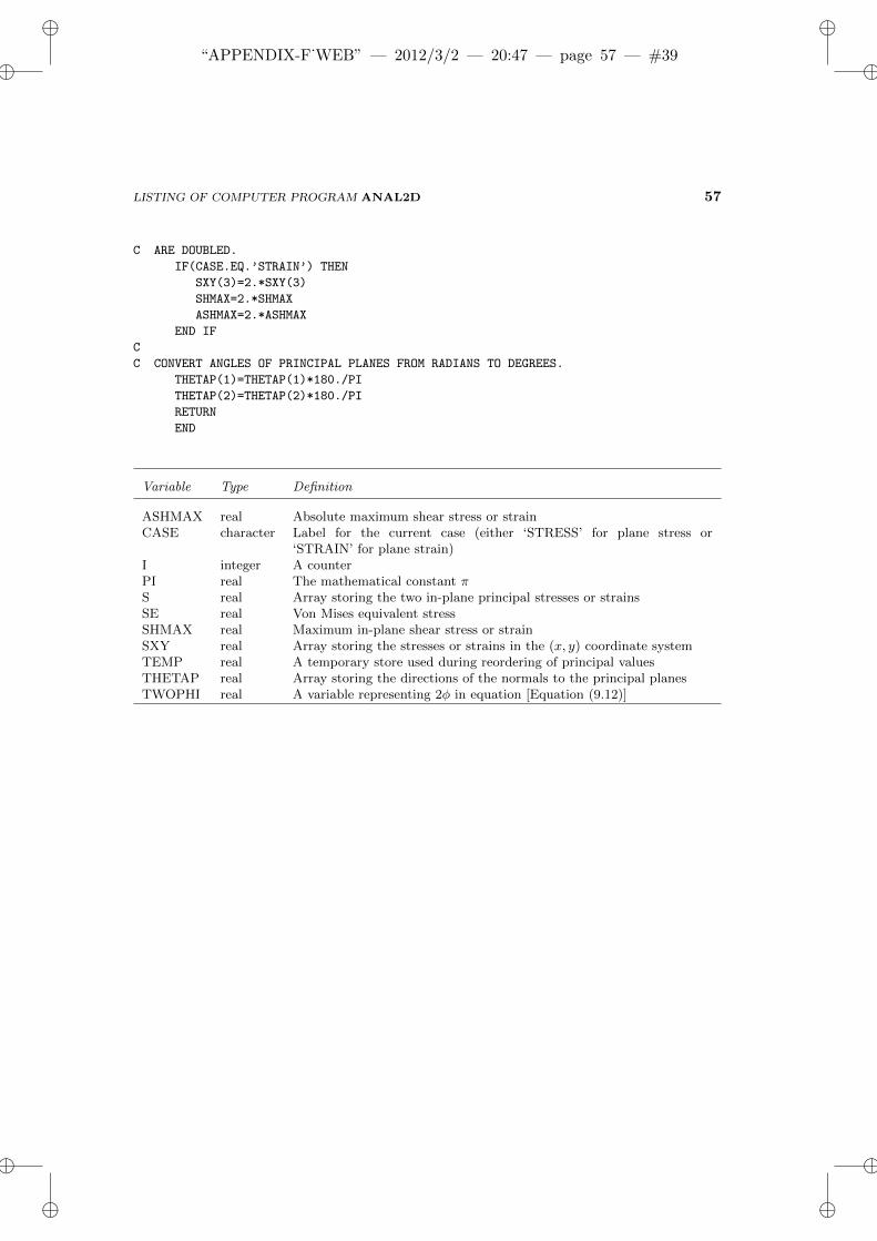
ii
“APPENDIX-F˙WEB” — 2012/3/2 — 20:47 — page 57 — #39 ii
ii
ii
LISTING OF COMPUTER PROGRAM ANAL2D 57
C ARE DOUBLED.
IF(CASE.EQ.’STRAIN’) THEN
SXY(3)=2.*SXY(3)
SHMAX=2.*SHMAX
ASHMAX=2.*ASHMAX
END IF
C
C CONVERT ANGLES OF PRINCIPAL PLANES FROM RADIANS TO DEGREES.
THETAP(1)=THETAP(1)*180./PI
THETAP(2)=THETAP(2)*180./PI
RETURN
END
Variable Type Definition
ASHMAX real Absolute maximum shear stress or strainCASE character Label for the current case (either ‘STRESS’ for plane stress or
‘STRAIN’ for plane strain)I integer A counterPI real The mathematical constant πS real Array storing the two in-plane principal stresses or strainsSE real Von Mises equivalent stressSHMAX real Maximum in-plane shear stress or strainSXY real Array storing the stresses or strains in the (x, y) coordinate systemTEMP real A temporary store used during reordering of principal valuesTHETAP real Array storing the directions of the normals to the principal planesTWOPHI real A variable representing 2φ in equation [Equation (9.12)]
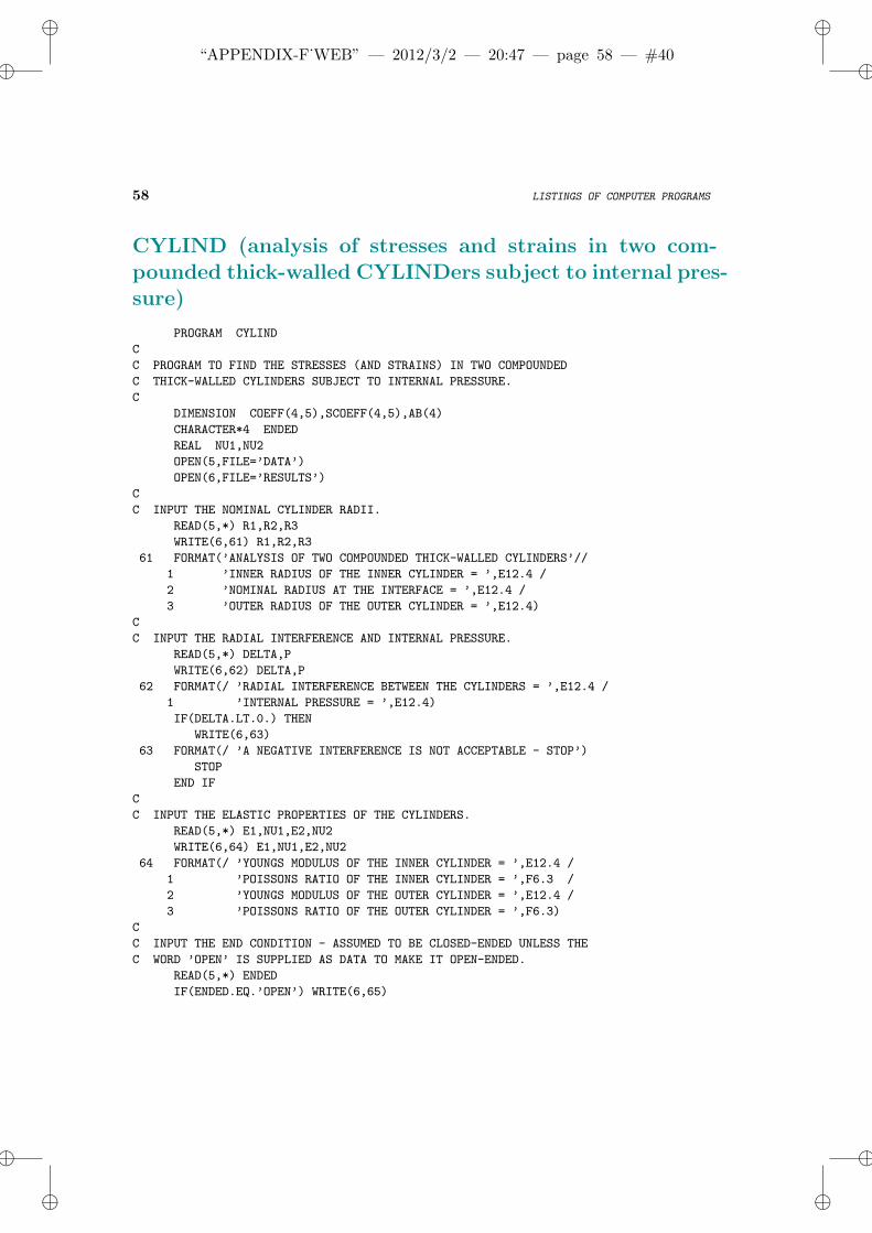
ii
“APPENDIX-F˙WEB” — 2012/3/2 — 20:47 — page 58 — #40 ii
ii
ii
58 LISTINGS OF COMPUTER PROGRAMS
CYLIND (analysis of stresses and strains in two com-pounded thick-walled CYLINDers subject to internal pres-sure)
PROGRAM CYLIND
C
C PROGRAM TO FIND THE STRESSES (AND STRAINS) IN TWO COMPOUNDED
C THICK-WALLED CYLINDERS SUBJECT TO INTERNAL PRESSURE.
C
DIMENSION COEFF(4,5),SCOEFF(4,5),AB(4)
CHARACTER*4 ENDED
REAL NU1,NU2
OPEN(5,FILE=’DATA’)
OPEN(6,FILE=’RESULTS’)
C
C INPUT THE NOMINAL CYLINDER RADII.
READ(5,*) R1,R2,R3
WRITE(6,61) R1,R2,R3
61 FORMAT(’ANALYSIS OF TWO COMPOUNDED THICK-WALLED CYLINDERS’//
1 ’INNER RADIUS OF THE INNER CYLINDER = ’,E12.4 /
2 ’NOMINAL RADIUS AT THE INTERFACE = ’,E12.4 /
3 ’OUTER RADIUS OF THE OUTER CYLINDER = ’,E12.4)
C
C INPUT THE RADIAL INTERFERENCE AND INTERNAL PRESSURE.
READ(5,*) DELTA,P
WRITE(6,62) DELTA,P
62 FORMAT(/ ’RADIAL INTERFERENCE BETWEEN THE CYLINDERS = ’,E12.4 /
1 ’INTERNAL PRESSURE = ’,E12.4)
IF(DELTA.LT.0.) THEN
WRITE(6,63)
63 FORMAT(/ ’A NEGATIVE INTERFERENCE IS NOT ACCEPTABLE - STOP’)
STOP
END IF
C
C INPUT THE ELASTIC PROPERTIES OF THE CYLINDERS.
READ(5,*) E1,NU1,E2,NU2
WRITE(6,64) E1,NU1,E2,NU2
64 FORMAT(/ ’YOUNGS MODULUS OF THE INNER CYLINDER = ’,E12.4 /
1 ’POISSONS RATIO OF THE INNER CYLINDER = ’,F6.3 /
2 ’YOUNGS MODULUS OF THE OUTER CYLINDER = ’,E12.4 /
3 ’POISSONS RATIO OF THE OUTER CYLINDER = ’,F6.3)
C
C INPUT THE END CONDITION - ASSUMED TO BE CLOSED-ENDED UNLESS THE
C WORD ’OPEN’ IS SUPPLIED AS DATA TO MAKE IT OPEN-ENDED.
READ(5,*) ENDED
IF(ENDED.EQ.’OPEN’) WRITE(6,65)
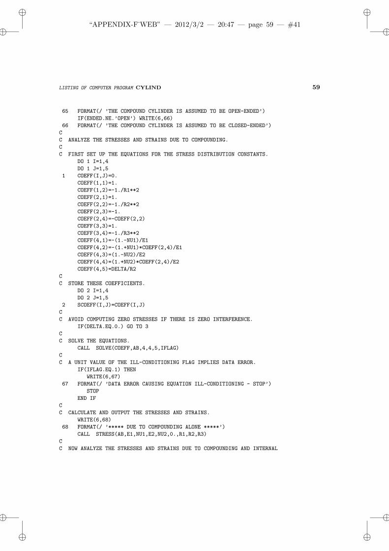
ii
“APPENDIX-F˙WEB” — 2012/3/2 — 20:47 — page 59 — #41 ii
ii
ii
LISTING OF COMPUTER PROGRAM CYLIND 59
65 FORMAT(/ ’THE COMPOUND CYLINDER IS ASSUMED TO BE OPEN-ENDED’)
IF(ENDED.NE.’OPEN’) WRITE(6,66)
66 FORMAT(/ ’THE COMPOUND CYLINDER IS ASSUMED TO BE CLOSED-ENDED’)
C
C ANALYZE THE STRESSES AND STRAINS DUE TO COMPOUNDING.
C
C FIRST SET UP THE EQUATIONS FOR THE STRESS DISTRIBUTION CONSTANTS.
DO 1 I=1,4
DO 1 J=1,5
1 COEFF(I,J)=0.
COEFF(1,1)=1.
COEFF(1,2)=-1./R1**2
COEFF(2,1)=1.
COEFF(2,2)=-1./R2**2
COEFF(2,3)=-1.
COEFF(2,4)=-COEFF(2,2)
COEFF(3,3)=1.
COEFF(3,4)=-1./R3**2
COEFF(4,1)=-(1.-NU1)/E1
COEFF(4,2)=-(1.+NU1)*COEFF(2,4)/E1
COEFF(4,3)=(1.-NU2)/E2
COEFF(4,4)=(1.+NU2)*COEFF(2,4)/E2
COEFF(4,5)=DELTA/R2
C
C STORE THESE COEFFICIENTS.
DO 2 I=1,4
DO 2 J=1,5
2 SCOEFF(I,J)=COEFF(I,J)
C
C AVOID COMPUTING ZERO STRESSES IF THERE IS ZERO INTERFERENCE.
IF(DELTA.EQ.0.) GO TO 3
C
C SOLVE THE EQUATIONS.
CALL SOLVE(COEFF,AB,4,4,5,IFLAG)
C
C A UNIT VALUE OF THE ILL-CONDITIONING FLAG IMPLIES DATA ERROR.
IF(IFLAG.EQ.1) THEN
WRITE(6,67)
67 FORMAT(/ ’DATA ERROR CAUSING EQUATION ILL-CONDITIONING - STOP’)
STOP
END IF
C
C CALCULATE AND OUTPUT THE STRESSES AND STRAINS.
WRITE(6,68)
68 FORMAT(/ ’***** DUE TO COMPOUNDING ALONE *****’)
CALL STRESS(AB,E1,NU1,E2,NU2,0.,R1,R2,R3)
C
C NOW ANALYZE THE STRESSES AND STRAINS DUE TO COMPOUNDING AND INTERNAL
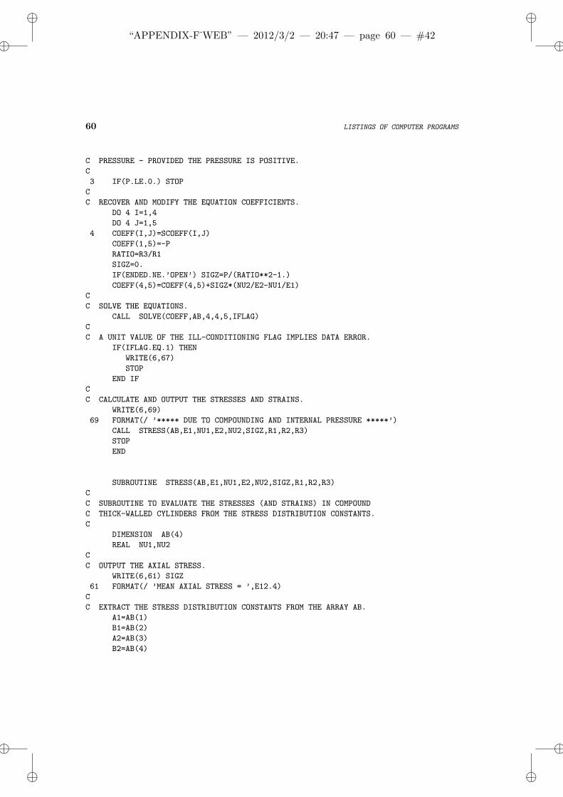
ii
“APPENDIX-F˙WEB” — 2012/3/2 — 20:47 — page 60 — #42 ii
ii
ii
60 LISTINGS OF COMPUTER PROGRAMS
C PRESSURE - PROVIDED THE PRESSURE IS POSITIVE.
C
3 IF(P.LE.0.) STOP
C
C RECOVER AND MODIFY THE EQUATION COEFFICIENTS.
DO 4 I=1,4
DO 4 J=1,5
4 COEFF(I,J)=SCOEFF(I,J)
COEFF(1,5)=-P
RATIO=R3/R1
SIGZ=0.
IF(ENDED.NE.’OPEN’) SIGZ=P/(RATIO**2-1.)
COEFF(4,5)=COEFF(4,5)+SIGZ*(NU2/E2-NU1/E1)
C
C SOLVE THE EQUATIONS.
CALL SOLVE(COEFF,AB,4,4,5,IFLAG)
C
C A UNIT VALUE OF THE ILL-CONDITIONING FLAG IMPLIES DATA ERROR.
IF(IFLAG.EQ.1) THEN
WRITE(6,67)
STOP
END IF
C
C CALCULATE AND OUTPUT THE STRESSES AND STRAINS.
WRITE(6,69)
69 FORMAT(/ ’***** DUE TO COMPOUNDING AND INTERNAL PRESSURE *****’)
CALL STRESS(AB,E1,NU1,E2,NU2,SIGZ,R1,R2,R3)
STOP
END
SUBROUTINE STRESS(AB,E1,NU1,E2,NU2,SIGZ,R1,R2,R3)
C
C SUBROUTINE TO EVALUATE THE STRESSES (AND STRAINS) IN COMPOUND
C THICK-WALLED CYLINDERS FROM THE STRESS DISTRIBUTION CONSTANTS.
C
DIMENSION AB(4)
REAL NU1,NU2
C
C OUTPUT THE AXIAL STRESS.
WRITE(6,61) SIGZ
61 FORMAT(/ ’MEAN AXIAL STRESS = ’,E12.4)
C
C EXTRACT THE STRESS DISTRIBUTION CONSTANTS FROM THE ARRAY AB.
A1=AB(1)
B1=AB(2)
A2=AB(3)
B2=AB(4)
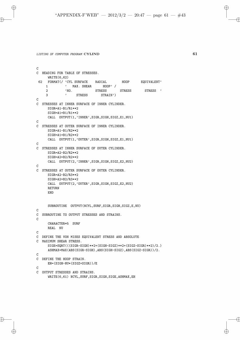
ii
“APPENDIX-F˙WEB” — 2012/3/2 — 20:47 — page 61 — #43 ii
ii
ii
LISTING OF COMPUTER PROGRAM CYLIND 61
C
C HEADING FOR TABLE OF STRESSES.
WRITE(6,62)
62 FORMAT(/ ’CYL SURFACE RADIAL HOOP EQUIVALENT’
1 ’ MAX. SHEAR HOOP’ /
2 ’NO. STRESS STRESS STRESS ’
3 ’ STRESS STRAIN’)
C
C STRESSES AT INNER SURFACE OF INNER CYLINDER.
SIGR=A1-B1/R1**2
SIGH=A1+B1/R1**2
CALL OUTPUT(1,’INNER’,SIGR,SIGH,SIGZ,E1,NU1)
C
C STRESSES AT OUTER SURFACE OF INNER CYLINDER.
SIGR=A1-B1/R2**2
SIGH=A1+B1/R2**2
CALL OUTPUT(1,’OUTER’,SIGR,SIGH,SIGZ,E1,NU1)
C
C STRESSES AT INNER SURFACE OF OUTER CYLINDER.
SIGR=A2-B2/R2**2
SIGH=A2+B2/R2**2
CALL OUTPUT(2,’INNER’,SIGR,SIGH,SIGZ,E2,NU2)
C
C STRESSES AT OUTER SURFACE OF OUTER CYLINDER.
SIGR=A2-B2/R3**2
SIGH=A2+B2/R3**2
CALL OUTPUT(2,’OUTER’,SIGR,SIGH,SIGZ,E2,NU2)
RETURN
END
SUBROUTINE OUTPUT(NCYL,SURF,SIGR,SIGH,SIGZ,E,NU)
C
C SUBROUTINE TO OUTPUT STRESSES AND STRAINS.
C
CHARACTER*5 SURF
REAL NU
C
C DEFINE THE VON MISES EQUIVALENT STRESS AND ABSOLUTE
C MAXIMUM SHEAR STRESS.
SIGE=SQRT(((SIGR-SIGH)**2+(SIGH-SIGZ)**2+(SIGZ-SIGR)**2)/2.)
ASHMAX=MAX(ABS(SIGR-SIGH),ABS(SIGH-SIGZ),ABS(SIGZ-SIGR))/2.
C
C DEFINE THE HOOP STRAIN.
EH=(SIGH-NU*(SIGZ+SIGR))/E
C
C OUTPUT STRESSES AND STRAINS.
WRITE(6,61) NCYL,SURF,SIGR,SIGH,SIGE,ASHMAX,EH
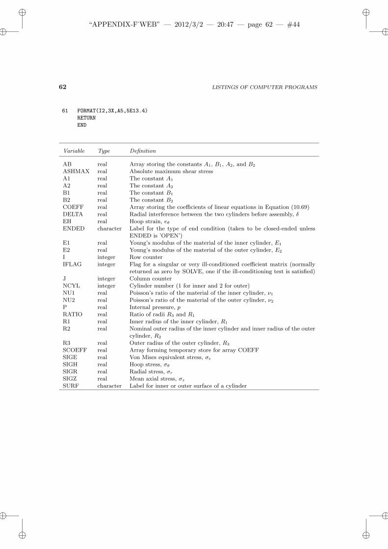
ii
“APPENDIX-F˙WEB” — 2012/3/2 — 20:47 — page 62 — #44 ii
ii
ii
62 LISTINGS OF COMPUTER PROGRAMS
61 FORMAT(I2,3X,A5,5E13.4)
RETURN
END
Variable Type Definition
AB real Array storing the constants A1, B1, A2, and B2
ASHMAX real Absolute maximum shear stressA1 real The constant A1
A2 real The constant A2
B1 real The constant B1
B2 real The constant B2
COEFF real Array storing the coefficients of linear equations in Equation (10.69)DELTA real Radial interference between the two cylinders before assembly, δEH real Hoop strain, eθENDED character Label for the type of end condition (taken to be closed-ended unless
ENDED is ’OPEN’)E1 real Young’s modulus of the material of the inner cylinder, E1
E2 real Young’s modulus of the material of the outer cylinder, E2
I integer Row counterIFLAG integer Flag for a singular or very ill-conditioned coefficient matrix (normally
returned as zero by SOLVE, one if the ill-conditioning test is satisfied)J integer Column counterNCYL integer Cylinder number (1 for inner and 2 for outer)NU1 real Poisson’s ratio of the material of the inner cylinder, ν1NU2 real Poisson’s ratio of the material of the outer cylinder, ν2P real Internal pressure, pRATIO real Ratio of radii R3 and R1
R1 real Inner radius of the inner cylinder, R1
R2 real Nominal outer radius of the inner cylinder and inner radius of the outercylinder, R2
R3 real Outer radius of the outer cylinder, R3
SCOEFF real Array forming temporary store for array COEFFSIGE real Von Mises equivalent stress, σeSIGH real Hoop stress, σθSIGR real Radial stress, σrSIGZ real Mean axial stress, σzSURF character Label for inner or outer surface of a cylinder