Embed Size (px)
Citation preview

Doctoral Dissertation on
Solution of Coupled Thermoelasticity Problem In Rotating Disks
byAyoob Entezari
26 September, 2017
Supervisors:Prof. M. A. Kouchakzadeh¹ and Prof. Erasmo Carrera²
¹Sharif University of TechnologyDepartment of Aerospace Engineering, Tehran, Iran
²Polytechnic University of Turin, Department of Mechanical and Aerospace Engineering, Italy
²MUL2 research group, Polytechnic University of Turin, Italy
Advisor:Dr. Matteo Filippi²
Cotutelle Doctoral Program

1. Introduction to rotating disks
2. Fundamentals of Linear Thermoelasticity
3. Literature review & present work
4. Analytical approach
5. Numerical approach
6. Conclusion
Outlines
1. Introduction to rotating disks
2. Fundamentals of Linear Thermoelasticity
3. Literature review & present work
4. Analytical approach
5. Numerical approach
6. Conclusion
Outlines

4
Aerospace (aero-engines, turbo-pumps, turbo-chargers, etc.)
Mechanical (spindles, flywheel, brake disks, etc.)
Naval
Power plant (steam and gas turbines, turbo-generators, )
Chemical plant
Electronics (electrical machines)
Applications
Introduction to rotating disks

5
Introduction to rotating disksConfigurations

6
Transient thermal load
In some of applications, the disks may be exposed to sudden temperature changes in short periods of time (for Ex. start and stop cycles)
These sudden changes in temperature can cause time dependent thermal stresses.
Thermal stresses due to large temperature gradients are higher than the steady-state stresses.
In such conditions, the disk should be designed with consideration of transient effects.
start and stop cyclesI) start up,
II) shut down
Introduction to rotating disksOperating conditions
Main Loads
Centrifugal forces
Thermal loads.

7
Effective properties of FGMs
ceramic-metal FGM
Metals: steels, super alloys
Ceramic matrix composites (CMC)
Functionally graded materials (FGMs)
Introduction to rotating disksDisk materials
Peff= VmPm +Vc Pc =Vm (Pm−Pc)+Pc
ceramic-metal FGM
Pm and Pc : properties of metal and ceramicVm and Vc : volume fractions of metal and ceramicVm = ( , , )

8
Introduction to rotating disksFGM disk
power gradation law for metal volume fraction along the radius
Vm = −−
met
al v
olum
e fra
ctio
n
radius
Effective properties of FGMs
Peff= VmPm +Vc Pc =Vm (Pm−Pc)+Pc

1. Introduction to rotating disk
2. Fundamentals of Linear Thermoelasticity
3. Literature review & present work
4. Analytical approach
5. Numerical approach
6. Conclusion
Outlines

10
Fundamentals of Linear Thermoelasticity
Inertia effects• static problems• dynamic problems
displacement and temperature fields interaction• uncoupled problems• coupled problems
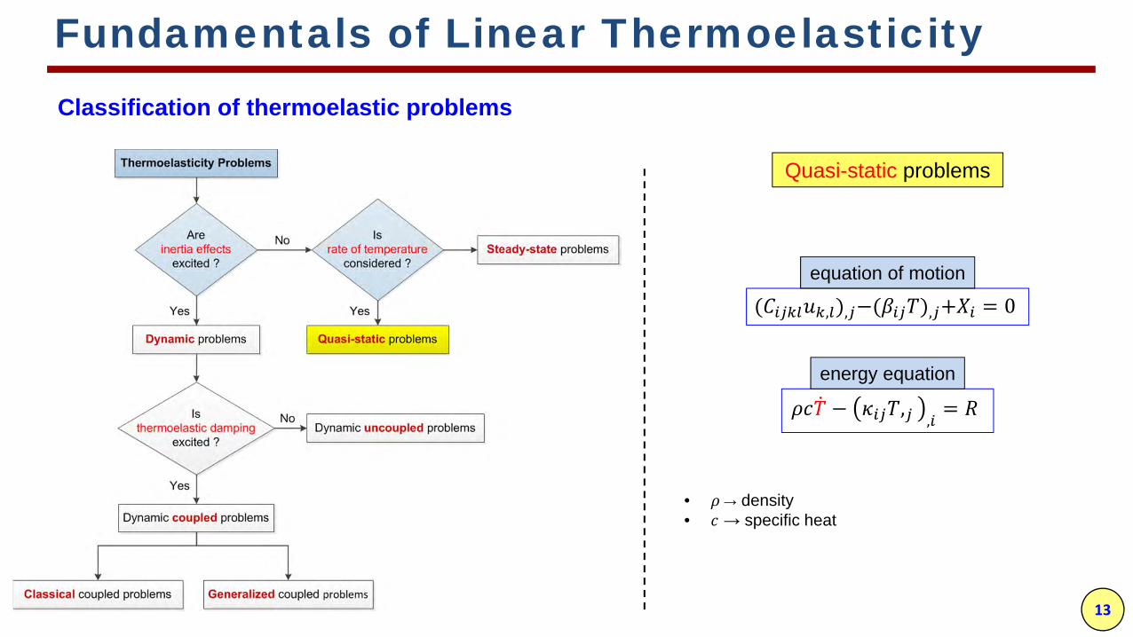
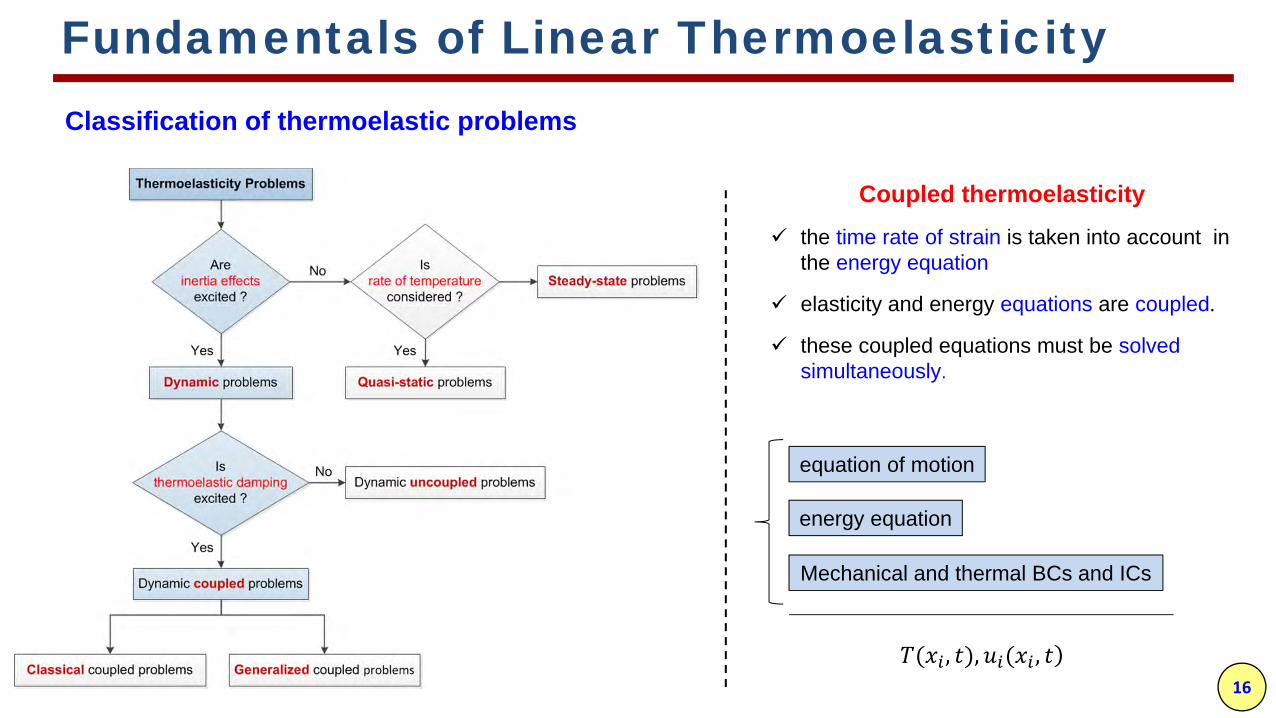
Classification of thermoelastic problems

11
( , ), −( ), + = 0equation of motion
energy equation( , ), =
Fundamentals of Linear ThermoelasticityClassification of thermoelastic problems
static steady-state problems
• → temperature change• → displacements• → elastic coefficients• → body forces• → thermoelastic moduli• → thermal conductivity• → internal heat source

12
Fundamentals of Linear ThermoelasticityClassification of thermoelastic problems
Under axisymmetric & plane stress assumptions
( ) = + ( ⁄ ) ln( ⁄ )
ℎ − ℎ + ℎ = 0
static steady-state problems
equation of motion
energy equation
13
− , , =
Fundamentals of Linear ThermoelasticityClassification of thermoelastic problems
Quasi-static problems
( , ), −( ), + = 0equation of motion
energy equation
• → density• → specific heat

14
( , ), −( ), + =− , , =
Fundamentals of Linear ThermoelasticityClassification of thermoelastic problems
equation of motion
energy equation
Dynamic uncoupled problems

15
( , ), −( ), + = +− , , =
Fundamentals of Linear ThermoelasticityClassification of thermoelastic problems
equation of motion
energy equation
Dynamic uncoupled problems
Considering mechanical damping
• → mechanical damping coefficient of material
16
Fundamentals of Linear Thermoelasticity
Coupled thermoelasticity
the time rate of strain is taken into account in the energy equation
elasticity and energy equations are coupled.
these coupled equations must be solved simultaneously.
Classification of thermoelastic problems
equation of motion
energy equation
Mechanical and thermal BCs and ICs
( , ), ( , )

17
( , ), −( ), + =− , , + , =
Fundamentals of Linear ThermoelasticityClassification of thermoelastic problems
equation of motion
energy equation
Classical coupled problems
• → reference temperature

18
( , ), −( ), + =− , , + , =
Fundamentals of Linear ThermoelasticityClassification of thermoelastic problems
equation of motion
energy equation
Classical coupled problems
→ reference temperature
infinite propagation speed for the thermal disturbances !!!

19
Fundamentals of Linear ThermoelasticityClassification of thermoelastic problems
in the classical thermoelasticity
heat conduction equation is of a parabolictype.
Predicting infinite speed for heat propagation
The prediction is not physically acceptable.
thermal wave disturbances are not detectable.
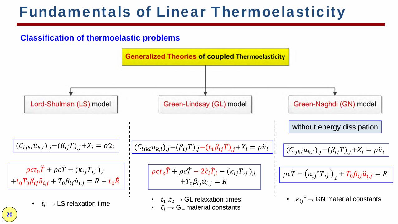
generalized theories of thermoelasticity
non-classical theories with the finite speed of the thermal wave.
20
( , ), −( ), + =+ − ( , ),+ , + , = +
( , ), −( ), −( ), + =+ − 2 , − ( , ),+ , =
( , ), −( ), + =− ∗ , , + , =
without energy dissipation
Fundamentals of Linear ThermoelasticityClassification of thermoelastic problems
• → LS relaxation time • , → GL relaxation times• → GL material constants
• ∗→ GN material constants
1. Introduction to rotating disk
2. Fundamentals of Linear Thermoelasticity
3. Literature review & present work
4. Analytical approach
5. Numerical approach
6. Conclusion
Outlines

22
Coupled thermoelasticity problems are still topics of active research.
Analytical solution of the these problems are mathematically difficult.
Number of papers on analytical solutions is limited.
Numerical methods are often used to solve these problems.
Numerical solutions of these problems have been presented in many articles.
Finite element method is still applied as a powerful numerical tool in such problems.
The major presented solutions are related to the basic problems (infinite medium, half-space, layer and axisymmetric problems).
Analytical and numerical solution of rotating disk problems has never before been presented.
Literature review & present work
Conclusion of the literature review

23
Literature review & present work
Present work
Study of coupled thermoelastic behavior in disks subjected to thermal shock loads
based on the generalized and classic theories
Disks with constant and variable thickness
Made of FGM
• Main purpose
• Implementation
Analytical approach
Numerical approach

24
1. Introduction to rotating disk
2. Fundamentals of Linear Thermoelasticity
3. Literature review & present work
4. Analytical approach
Solution method
Numerical evaluation
5. Numerical approach
6. Conclusion
Outlines

25
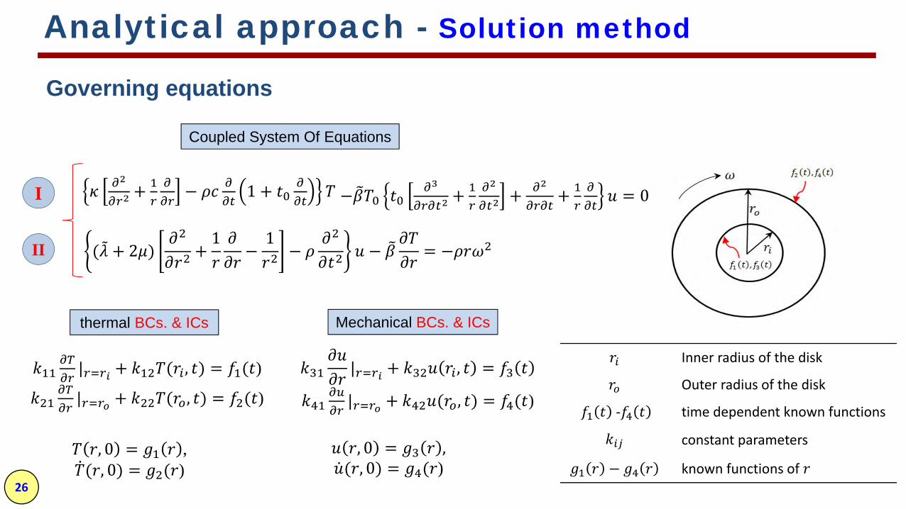
Consider• An annular rotating disk with constant thickness, • made of isotropic & homogeneous material, • Under axisymmetric thermal and mechanical shock loads.
Analytical approach - Solution method
Governing equations
( , ), −( ), + =+ − ( , ),+ , + , = +
+ 1 − 1 +− + 1 + + 1 = 0
( + 2 ) + 1 − 1 − − = −
Based on LS generalized coupled theory
Eq. of motion
energy Eq.
= 2+ 2 = 2+ 2 3 + 2 • & → Lame constants• → coefficient of linear thermal expansion
I
II
26
Analytical approach - Solution method
Governing equations
+ − 1 +
− + + + = 0( + 2 ) + 1 − 1 − − = −
Inner radius of the disk
Outer radius of the disk
- time dependent known functions
constant parameters − known functions of , 0 = ,( , 0) = ( )
, 0 = ,( , 0) = ( )
| + , =| + ( , ) = ( )
| + ( , ) = ( )| + ( , ) = ( )
thermal BCs. & ICs Mechanical BCs. & ICs
Coupled System Of Equations
I
II

27
propagation speed of elastic longitudinal wave
Analytical approach - Solution method
Governing equations in Non-dimensional form
Non-dimensional parameters
unit length
= + 2 )⁄= ⁄
= , = , == , = , == + 2 ) , =

28
Thermoelastic damping or coupling parameter
where
Analytical approach - Solution method
Governing equations in Non-dimensional form
Coupled System Of Equations
I
II
+ 1 − 1 − − = − + 1 − 1 + − + 1 + + 1 = 0
= ( + 2• Non-dimensional propagation speed of thermal wave → = 1 ⁄• Non-dimensional propagation speed of elastic longitudinal wave → = 1

29
Analytical approach - Solution method
Solution of non-dimensional equations
Coupled System Of Equations
I
II
+ 1 − 1 − − = − + 1 − 1 + − + 1 + + 1 = 0
| + ( , ) = ( ) | + ( , ) = ( ) | + ( , ) = ( ) | + ( , ) = ( )( , 0) = ( ), ( , 0) = ( )( , 0) = ( ), ( , 0) = ( )
Thermal and mechanical BCs. & ICs

30
Analytical approach - Solution method
+ 1 − 1 + − + 1 + + 1 = 0Solution of non-dimensional equations
energy Eq.
+ 1 − − = 0| + ( , ) = ( ) | + ( , ) = ( )( , 0) = 0 , ( , 0) = 0
+ 1 − − = , + + , +| + ( , ) = 0 | + ( , ) = 0( , 0) = ( ) , ( , 0) = ( )
( , ) = ( , ) + ( , )principle of superposition
decomposition

31
Analytical approach - Solution method
Solution of non-dimensional equations
principle of superposition
decomposition
( , ) = ( , ) + ( , )
+ 1 − 1 − − = − Eq. of motion
+ 1 − − = 0| + ( , ) = ( ) | + ( , ) = ( )( , 0) = 0 , ( , 0) = 0
+ 1 − − = , −| + ( , ) = 0 | + ( , ) = 0( , 0) = ( ) , ( , 0) = ( )

32
Analytical approach - Solution method
Solution of non-dimensional equations
Bessel equation and can beseparately solved using finite Hankel transform
decomposition
+ 1 − 1 − − = − Eq. of motion
+ 1 − − = 0| + ( , ) = ( ) | + ( , ) = ( )( , 0) = 0 , ( , 0) = 0
+ 1 − − = , −| + ( , ) = 0 | + ( , ) = 0( , 0) = ( ) , ( , 0) = ( )

33
and are positive roots of the following equations
Analytical approach - Solution method
Finite Hankel transform
Solution of non-dimensional equations
kernel functions
ℋ[ ( , )] = ( , ) = ( , ) ( , )ℋ[ ( , )] = ( , ) = ( , ) ( , )
( , ) = ( ) ( ) | + ( − ( ) ( ) | + (( , ) = ( ) ( ) | + ( − ( ) ( ) | + (
( ) | + ( ( ) | + ( − ( ) | + ( ( ) | + (= 0( ) | + ( ( ) | + ( − ( ) | + ( ( ) | + ( = 0

34
2 20 1 1 1 2 1
1
2( ) ( )m
dt T T T f t f t
dx
p
æ ö÷ç ÷+ + = -ç ÷ç ÷è ø 2 4
1 1 4 33
2( ) ( )n
du u f t f t
dh
p
æ ö÷ç ÷+ = -ç ÷ç ÷è ø
21 1 1
12 2
131 32 1 3
141 42 1 4
1 1
10
( , ) ( )
( , ) ( )
( , 0) 0 , ( , 0) 0
r a
r b
u u uu
r rr r
uk k u a t f t
ru
k k u b t f tr
u r u r
=
=
¶ ¶+ - - =
¶¶
¶+ =
¶¶
+ =
= =
21 1
1 0 12
111 12 1 1
121 22 1 2
1 1
10
( , ) ( )
( , ) ( )
( , 0 ) 0 , ( , 0 ) 0
r a
r b
T TT t T
r rr
Tk k T a t f t
rT
k k T b t f tr
T r T r
=
=
¶ ¶+ - - =
¶¶
¶+ =
¶¶
+ =
= =
Taking the finite Hankel transform
Analytical approach - Solution method
Uncoupled sub-IBVPs (Bessel equations)
Solution of non-dimensional equations
Solving ODEs
1( , )nu t h 1( , )mT t x

35
2 20 1 1 1 2 1
1
2( ) ( )m
dt T T T f t f t
dx
p
æ ö÷ç ÷+ + = -ç ÷ç ÷è ø 2 4
1 1 4 33
2( ) ( )n
du u f t f t
dh
p
æ ö÷ç ÷+ = -ç ÷ç ÷è ø
Analytical approach - Solution method
Uncoupled sub-IBVPs (Bessel equations)
Solution of non-dimensional equations
Solving ODEs
1( , )nu t h 1( , )mT t x
Inverse finite Hankel transforms
= 1‖ ( , )‖ , = 1‖ ( , )‖
( , ) = ( , ) ( , ( , ) = ( , ) ( , )

36
Analytical approach - Solution method
Solution of non-dimensional equations
( , ) = ( ) ( , ) , ( , ) = ( ) ( , )
decomposition
+ 1 − 1 − − = − Eq. of motion
+ 1 − − = 0| + ( , ) = ( ) | + ( , ) = ( )( , 0) = 0 , ( , 0) = 0
+ 1 − − = , −| + ( , ) = 0 | + ( , ) = 0( , 0) = ( ) , ( , 0) = ( )

37
Analytical approach - Solution method
Solution of non-dimensional equations
Coupled System Of Equations
I
II
+ 1 − 1 − − = − + 1 − 1 + − + 1 + + 1 = 0
( , ) = ( , ) ( , ) + ( ) ( , )( , ) = ( , ) ( , + ( ) ( , )

1. Introduction to rotating disk
2. Fundamentals of Linear Thermoelasticity
3. Literature review & present work
4. Analytical approach
Solution method
Numerical evaluation
5. Numerical approach
6. Conclusion
Outlines

39
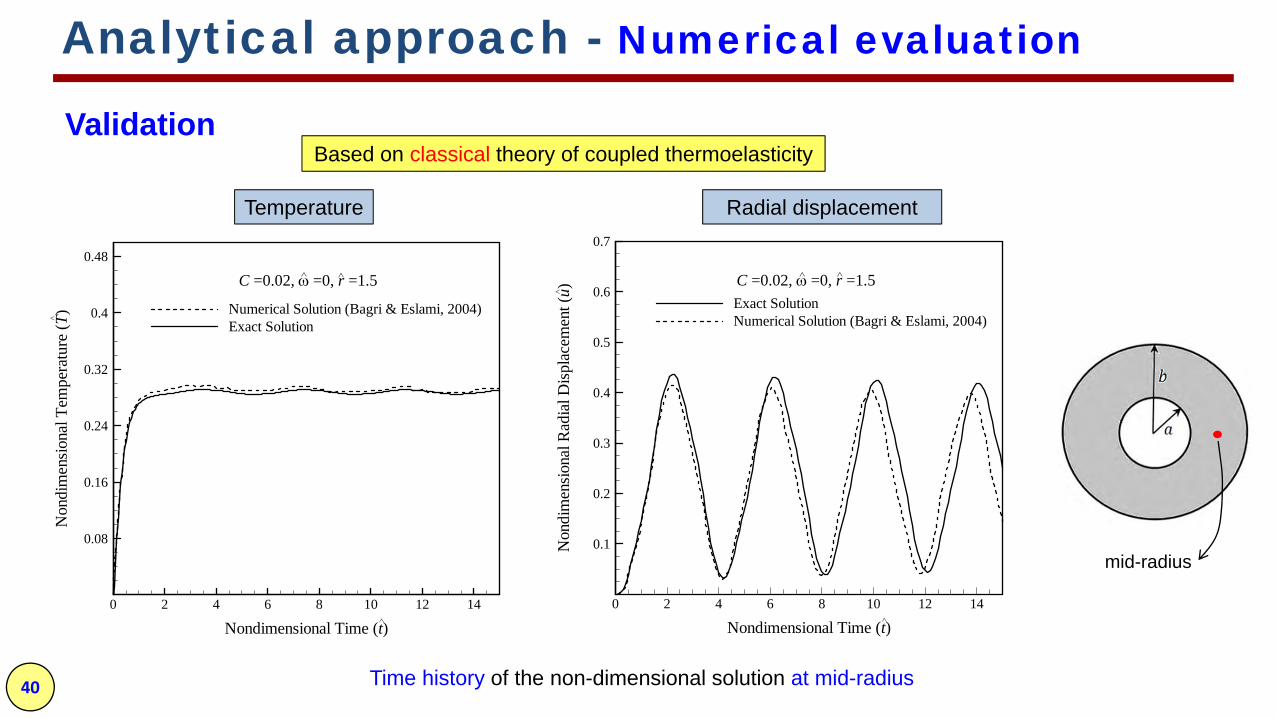
Analytical approach - Numerical evaluation
material properties
geometry
Specifications of numerical example
= 1= 2= 40.4 GPa= 27 GPa= 23 × 10 K= 2707 kg/m3= 204 W/m ⋅ K= 903 J/kg ⋅ K
( ) = 0 01 0
Boundary conditions
at = → − = ( )= 0at = → = 0= 0
40
Time history of the non-dimensional solution at mid-radius
Analytical approach - Numerical evaluation
Based on classical theory of coupled thermoelasticity
Temperature Radial displacement
mid-radius
Nondimensional Time (t)
Non
dim
ensio
nalT
empe
ratu
re(T
)
0 2 4 6 8 10 12 14
0.08
0.16
0.24
0.32
0.4
0.48
Numerical Solution (Bagri & Eslami, 2004)Exact Solution
C =0.02, =0, r =1.5
Nondimensional Time (t)
Non
dim
ensio
nalR
adia
lDisp
lace
men
t(u)
0 2 4 6 8 10 12 14
0.1
0.2
0.3
0.4
0.5
0.6
0.7
Exact SolutionNumerical Solution (Bagri & Eslami, 2004)
C =0.02, =0, r =1.5
Validation

41
Time history of the non-dimensional solution at mid-radius
Analytical approach - Numerical evaluation
Nondimensional Time (t)
Non
dim
ensio
nalT
empe
ratu
re(T
)
0 2 4 6 8 10 12 140
0.05
0.1
0.15
0.2
0.25
0.3
0.35
0.4
0.45
0.5
Exact SolutionNumerical (Bagri & Eslami, 2004)
t0 =0.64, C =0.02, =0, r =1.5
Nondimensional Time (t)
Non
dim
ensio
nalR
adia
lDisp
lace
men
t(u)
0 2 4 6 8 10 12 14
-0.2
-0.1
0
0.1
0.2
0.3
0.4
0.5
0.6
0.7
0.8
0.9
1
Exact SolutionNumerical (Bagri & Eslami, 2004)
t0 =0.64, C =0.02, =0, r =1.5
Temperature Radial displacement
mid-radius
Based on LS generalized theory of coupled thermoelasticityValidation

42
Analytical approach - Numerical evaluation
Nondimensional Radius(r)
Non
dim
ensio
nalT
empe
ratu
re(T
)
1 1.2 1.4 1.6 1.8 2
-0.1
0
0.1
0.2
0.3
0.4
0.5
0.6
0.7
0.8
steady state
T0=293 K, t0=0.64, =0.01
1.25
t=0.25
0.5
0.75
1
+
+
+
+
+
+
+
+
+
+
++
++
++
+ + + + + +
Nondimensional Radius (r)
Non
dim
ensio
nalR
adia
lDisp
lace
men
t(u)
1 1.2 1.4 1.6 1.8 2
-0.1
0
0.1
0.2
0.3
0.4
0.5
0.6
0.7
steady statet =0.25
1
T0=293 K, t0=0.64, =0.01
1.25
t =0.50.75
10
Nondimensional Radius (r)
Non
dim
ensio
nalT
ange
ntia
lStre
ss(
)
1 1.2 1.4 1.6 1.8 2
-0.7
-0.6
-0.5
-0.4
-0.3
-0.2
-0.1
0
0.1
0.2
steady statet = 0.25t = 0.5t = 0.75t = 1t = 1.25
T0=293 K, t0=0.64, =0.01
Nondimensional Radius (r)
Non
dim
ensio
nalR
adia
lStre
ss(
rr)
1.2 1.4 1.6 1.8 2
-0.7
-0.6
-0.5
-0.4
-0.3
-0.2
-0.1
0
0.1
steady statet = 0.25t = 0.5t = 0.75t = 1t = 1.25
T0=293 K, t0=0.64, =0.01
temperature change radial stress circumferential stressradial displacement
radius radius radius radius
Based on LS generalized theory of coupled thermoelasticity
Radial distribution for different values of the time.
Results and discussion

1. Introduction to rotating disk
2. Fundamentals of Linear Thermoelasticity
3. Literature review & present work
4. Analytical approach
5. Numerical approach
6. Conclusion
Outlines

1. Introduction to rotating disk
2. Fundamentals of Linear Thermoelasticity
3. Literature review & present work
4. Analytical approach
5. Numerical approach
Motivation
Development of method
Evaluations and results
6. Conclusion
Outlines

45
Analytical solutions are limited to those of a disk with simple geometry and boundary conditions.
FE method is more widely used for this class of problems.
1D and 2D FE models are not able to provide all the desired information.
3D FE modeling techniques may be required for a detailed coupled thermoelastic analysis.
3D FE models still impose large computational costs, specially, in a time-consuming transient solution.
There is a growing interest in the development of refined FE models with lower computational efforts.
A refined FE approach was developed by Prof. Carrera et al.
They formulated the FE methods on the basis of a class of theories of structures.
Numerical approach
Motivations

46
Numerical approachMain characteristics of FE models refined by Carrera
3D capabilities
lower computational costs
ability to analyze multi-field problems and multi-layered structuresMUL2 research group,Polytechnic University,
Turin, Italywww.mul2.polito.it

1. Introduction to rotating disk
2. Fundamentals of Linear Thermoelasticity
3. Literature review & present work
4. Analytical approach
5. Numerical approach
Motivation
Development of method
Evaluations and results
6. Conclusion
Outlines
48
Approaches to FE modeling
Numerical approach - Development of method
Variational approach
Weighted residual methods
Weighted residual method based on Galerkin technique
Efficient, high rate of convergence
most common method to obtain a weak formulation of the problem

49
Governing equations
, , ,, ,Equation of motion Energy equation
Numerical approach - Development of method
)Hooke’s law
For anisotropic and nonhomogeneous materials.
Including LS, GL and classical theories of thermoelasticity.
Considering mechanical damping effect.
= = = = 0 → classical theory
= = = 0→ LS theory
= 0→ GL theory.
50
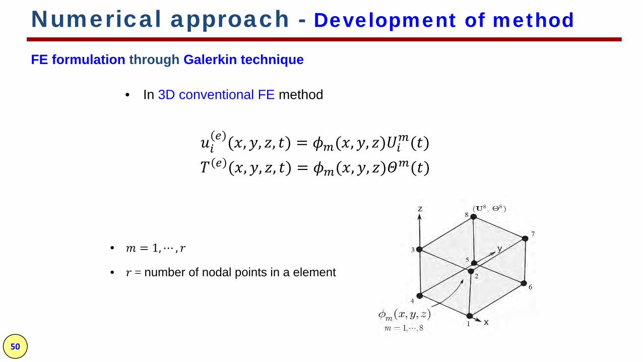
( , , , ) = ( , , ) ( )( , , , ) = ( , , ) ( )• = 1,⋯ ,• = number of nodal points in a element
Numerical approach - Development of method
FE formulation through Galerkin technique
• In 3D conventional FE method

51
, + − − = 0 ( + ) + − 2 , − , ,+ , + , − − = 0Equation of motion energy equation
Weighting function
Numerical approach - Development of method
FE formulation through Galerkin technique
( , , )

52
( ) + ( ) + ( T σ)= ( ) + ( )
( βT ) + ) + )+ ( βT ) + ) − (2 T∇ )
+ (∇T κ∇ ) = ( T ) + ( ) + )
Eq. of motion
energy Eq.
Numerical approach - Development of method
FE formulation through Galerkin technique
53
Numerical approach - Development of method
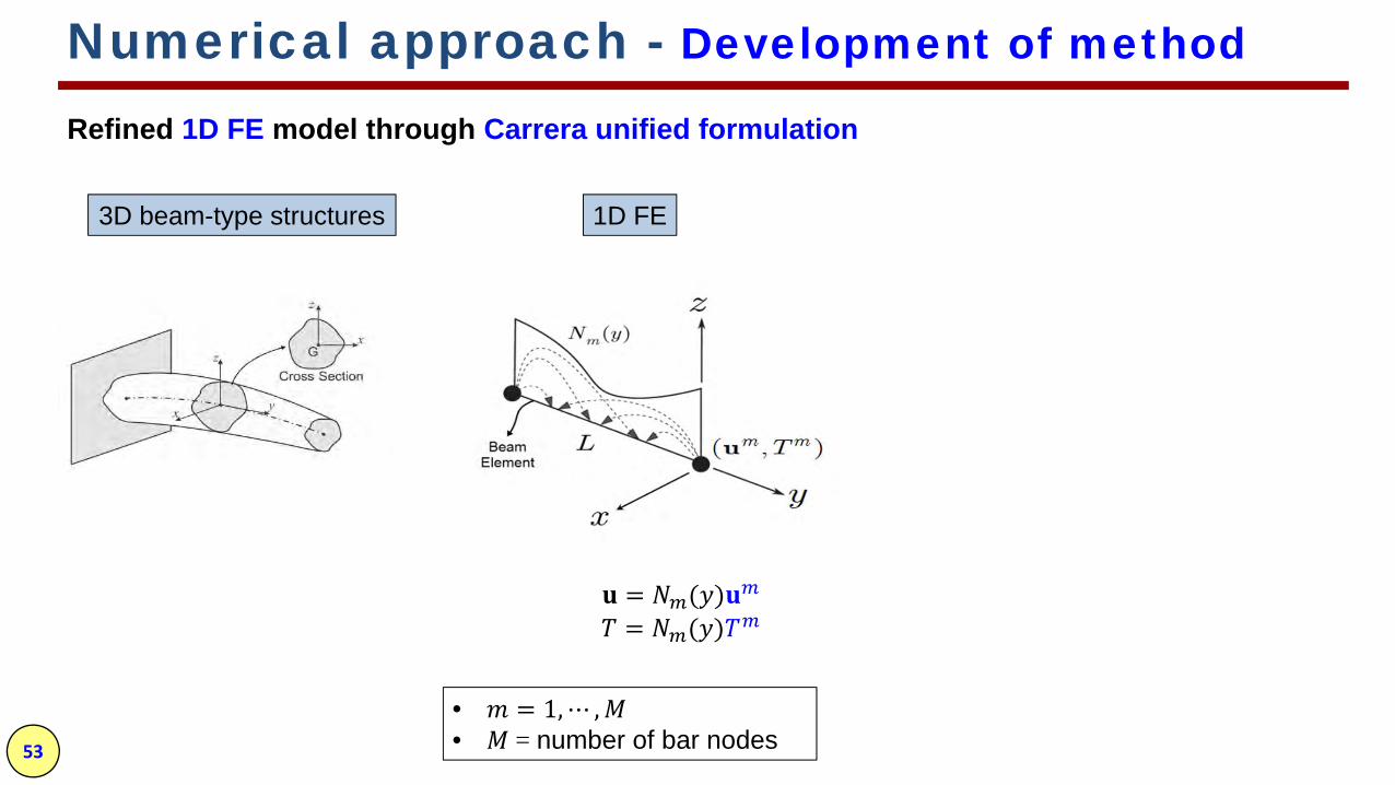
Refined 1D FE model through Carrera unified formulation
= ( )= ( )
1D FE3D beam-type structures
• = 1,⋯ ,• = number of bar nodes

54
• = 1,⋯ ,• = number of terms of the expansion.
Carrera unified formulation (CUF)
( , ) = ( , ) ( )( , ) = ( , )Θ ( )
Numerical approach - Development of method
Refined 1D FE model through Carrera unified formulation
• = 1,⋯ ,• = number of bar nodes
= ( )= ( )
1D FE3D beam-type structures

55
= ( )= ( )1D FE CUF( , ) = ( , ) ( )( , ) = ( , )Θ ( ) ( , , , ) = ( , , ) ( )( , , , ) = ( , , ) Θ ( )
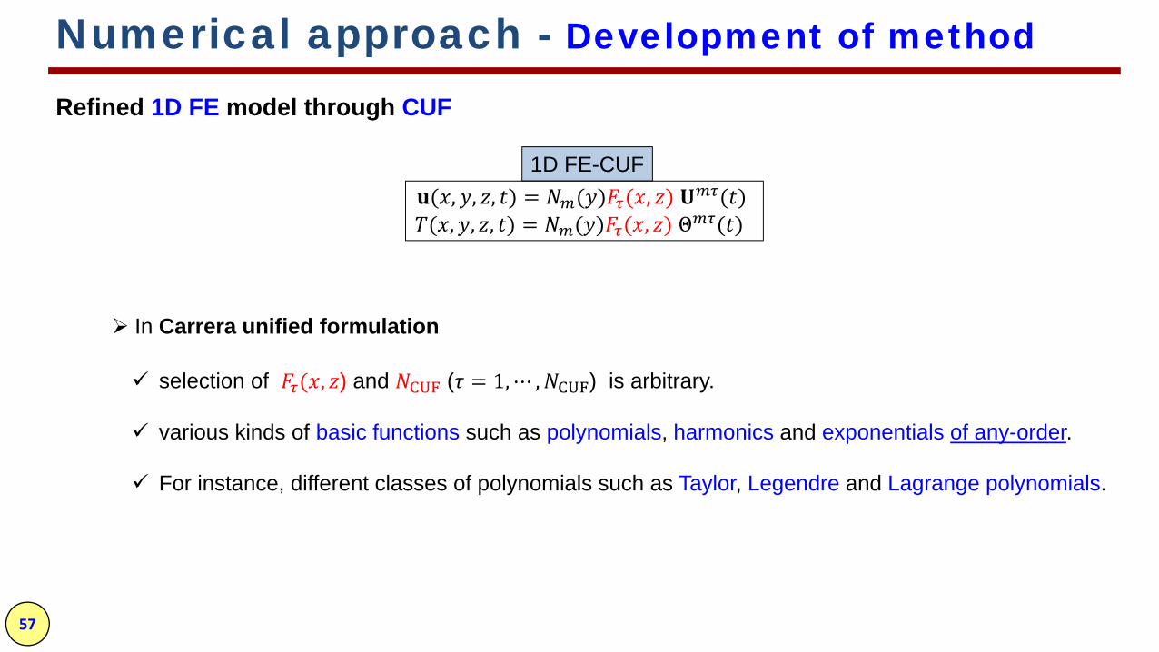
1D FE-CUF
3D 8-nodes elementrefined 1D 2-nodes element
Numerical approach - Development of method
Refined 1D FE model through CUF
weighting function in 1D FE-CUF → ( , , )= ( ) ( , )

56
Numerical approach - Development of method
Refined 1D FE model through CUF
( , , , ) = ( ) ( , ) ( )( , , , ) = ( ) ( , ) Θ ( )1D FE-CUF
1D FE modeling elements and shape functions in 1D FE modeling
B2 linear
element
B2 quadratic
B4 cubic
57
selection of ( , ) and ( = 1,⋯ , ) is arbitrary.
various kinds of basic functions such as polynomials, harmonics and exponentials of any-order.
For instance, different classes of polynomials such as Taylor, Legendre and Lagrange polynomials.
In Carrera unified formulation
Numerical approach - Development of method
Refined 1D FE model through CUF
( , , , ) = ( ) ( , ) ( )( , , , ) = ( ) ( , ) Θ ( )1D FE-CUF

58
( , ) → bi-dimensional Lagrange functions
cross-sections can be discretized using Lagrange elements
• linear three-point (L3)• quadratic six-point (L6) • bilinear four-point (L4)
Numerical approach - Development of method
Refined 1D FE model through CUF
( , , , ) = ( ) ( , ) ( )( , , , ) = ( ) ( , ) Θ ( )1D FE-CUF
• biquadratic nine-point (L9) • bi-cubic sixteen-point (L16)

59
Substituting
into the weak forms of equation of motion and energy equation gives
lm s ls lm s ls lm s ls mt t t t+ =+M G K p d d d
• , and → 4×4 fundamental nuclei (FNs)of the mass, damping, and stiffness matrices
• → 4×1 FN of the load vector
• δ → 4×1 FN of the unknowns vector
Numerical approach - Development of method
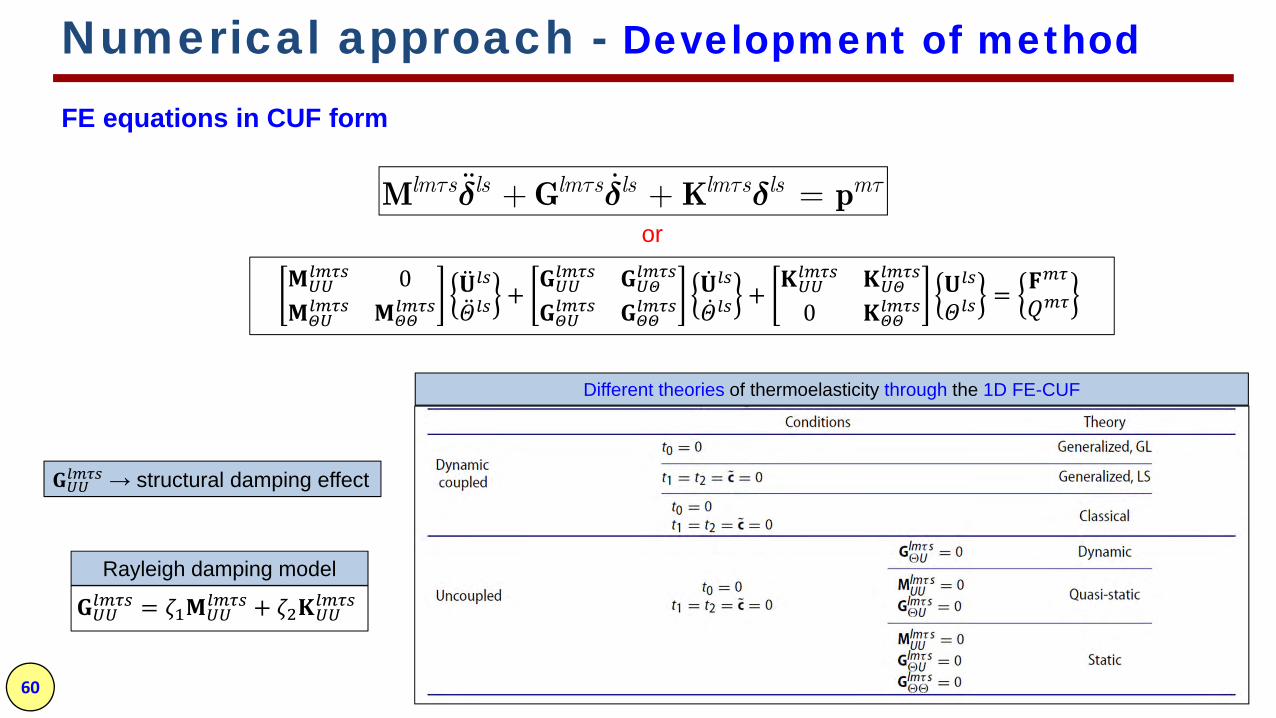
FE equations in CUF form
( , , , ) = ( ) ( , ) ( )( , , , ) = ( ) ( , ) Θ ( )1D FE-CUF ( , , )= ( ) ( , )weighting function
60
Rayleigh damping model
→ structural damping effect
or
Numerical approach - Development of method
0 + + 0 =
= +
lm s ls lm s ls lm s ls mt t t t+ =+M G K p d d d
FE equations in CUF form
Different theories of thermoelasticity through the 1D FE-CUF

61
+ + =M G K P D D Dfor whole structure
assembly procedure of FNsfor each elementlm s ls lm s ls lm s ls mt t t t=+ +M G K pd d d
2 L4
3 B4
Numerical approach - Development of method
total degrees of freedom
DOF = 4 ×a model with 3 B4 / 2 L4, DOF=240
Assembly procedure via Fundamental Nuclei

62
taking Laplace
Transfinite element technique
2[ ]lm seq
lm s lm s lm s ls ms st
t t t t* *+ + =
K
M G pK d
numerical inversion
Numerical approach - Development of method
Time history analysis
lm s ls lm s ls lm s ls mt t t t=+ +M G K pd d d
eq* *=K PD
Assembling & ∗ for whole structure
solution in Laplace domain Δ∗solve
solution in time domain (Δ( ))
• →the Laplace variable• → FN of the equivalent stiffness matrix• ∗ denotes Laplace transform of the terms.

63
diffusivity velocity of elastic longitudinal wave unit length
Numerical approach - Development of method
Non-dimensional Equation for isotropic FGMs
Non-dimensional parameters
m
m
m
m m
m m0 0
m m m
m m m m
m m
m m m
ˆˆ ; ;
( 2 )ˆ ˆˆ; ;
1 1 1ˆˆ ˆ; ;
ˆ ˆ;( 2 )
eii
ei i
d d
n ni i ij ij i i
d e d d
i id m d
Vxx t t
l l
VTT u u t t
T l T l
q q t tc T V T T
l DX X R R
T c T
l mb
s sr b b
b l m
= =
+= = =
= = =
= =+
m m m m( 2 )/eV l m r= +mm m / el D V= m m m m/D ck r=

64
Numerical approach - Development of method
δ ∗ = ∗or ∗∗∗∗
=∗∗∗∗
Non-dimensional FNs for isotropic FGMs based on LS theory
Transfinite element equation2
11 22 , ,
, ,66 44 , ,
, ,12 66 , 23 ,
13 44 , , 21 , ,
14 ,
41
ˆ ˆ
ˆ ˆ
ˆ ˆ
ˆ ˆ
ˆ
y y
y y
slm ml mls L x s x L
m l mls L z s z L
m l mlslms x L x s L
slm ml mlz s x L x s z L
slm mlx s L
s
K s C F F I C F F I
C F F I C F F I
K C F F I C F F I
K C F F I C F F I
K C F F I
K
tr t t
t t
tt t
tt t
tb t
t
= +
+ +
= +
= +
=-
20 ,
,242 0
243 0 ,
244 0
, ,, ,
, ,
ˆˆ( )
ˆˆ( )
ˆˆ( )
ˆ ˆˆ( )
ˆ ˆ
ˆ
y
y y
lm mls x L
mlslms L
slm mls z L
slm mlc s L
m lmlx s x L s L
mlz s z L
C s t s C F F I
K C s t s C F F I
K C s t s C F F I
K s t s C C F F I
C F F I C F F I
C F F I
b t
tb t
tb t
tr t
k t k t
k t
= +
= +
= +
= + +
+ +
+
( ) ( )
( ) ( )
( ) ( )
( ) ( )
*1
*2
*3
* *4 0
ˆt
ˆt
ˆt
ˆˆ ˆ[( 1) ] ( )
e e
e e
e e
e e
m nx m x m
S Vm n
y m y m
S Vm n
z m z m
S Vm
m i i m
V S
p F N dS X F N dV
p F N dS X F N dV
p F N dS X F N dV
p t s R F N dV q n F N dS
tt t
tt t
tt t
tt t
* *
* *
* *
*
= +
= +
= +
= + +
ò ò
ò ò
ò ò
ò ò

65
Numerical approach - Development of method
Non-dimensional FNs for isotropic FGMs based on LS theory
11 22 , ,
, ,66 44 , ,
, ,12 66 , 23 ,
2
13 44 , , 21 , ,
14 ,
41
ˆ ˆ
ˆ ˆ
ˆ ˆ
ˆ ˆ
ˆ
y y
y y
slm ml mls L x s x L
m l mls L z s z L
m l mlslms x L x s L
slm ml mlz s x L x s z L
slm mlx s L
s
K C F F I C F F I
C F F I C F F I
K C F F I C F F I
K C F F I C F F I
K C F I
s
F
K
tr t t
t t
tt t
tt t
tb t
t
= +
+ +
= +
= +
=-
0 ,
,42 0
43 0 ,
44 0
, ,, ,
,
2
2
,
2
2
ˆˆ( )
ˆˆ( )
ˆˆ( )
ˆ ˆˆ( )
ˆ ˆ
ˆ
y
y y
lm mls x L
mlslms L
slm mls z L
slm mlc s L
m lmlx s x L s L
mlz s z L
s t C F F I
K t C F F I
K t C F F I
K t C C F F I
C F F I C F F I
C F F I
C
C
C
s
s s
s s
s s
b t
tb t
tb t
tr t
k t k t
k t
= +
= +
= +
= + +
+ +
+
( )( )
eAdA= ò
( )( ) , , , ,
, , , ,y y y y
e y y y y
m l ml m lmlL L L L m l m l m l m lLI I I I N N N N N N N N dy=ò
( )11 22 33
m m
44 55 66m m
12 13 23m m
2ˆ ˆ ˆ( 2 )
ˆ ˆ ˆ( 2 )
ˆ ˆ ˆ( 2 )
C C C
C C C
C C C
m l
l mm
l ml
l m
+= = =
+
= = =+
= = =+
m m m m
ˆ ˆ ˆ ˆ, , , cc
C C C Ccr b k
r b kr b k
= = = =
20 m
m m m m( )
T
cC
br l m
=+
thermoelastic coupling parameter →

1. Introduction to rotating disk
2. Fundamentals of Linear Thermoelasticity
3. Literature review & present work
4. Analytical approach
5. Numerical approach
Motivation
Development of method
Evaluations and results
6. Conclusion
Outlines

1. Introduction to rotating disk2. Fundamentals of Linear Thermoelasticity3. Literature review & present work4. Analytical approach5. Numerical approach Motivation Development of method Evaluations and results
o Static structural analysisExample 1. Rotating variable thickness diskExample 2. Rotating variable thickness disk subjected thermal loadExample 3. Complex rotor
o Static structural-thermal analysis – Example 4. simple beam
o Quasi-static structural-thermal analysis – Example 5. simple beam
o Dynamic coupled structural-thermal analysisExample 6. Constant thickness disk made of isotropic homogeneous materialsExample 7. Constant thickness disk made of isotropic FGMs Example 8. variable thickness disk made of isotropic FGMs
6. Conclusion
Outlines

1. Introduction to rotating disk2. Fundamentals of Linear Thermoelasticity3. Literature review & present work4. Analytical approach5. Numerical approach Motivation Development of method Evaluations and results
o Static structural analysisExample 1. Rotating variable thickness diskExample 2. Rotating variable thickness disk subjected thermal loadExample 3. Complex rotor
o Static structural-thermal analysis – Example 4. simple beam
o Quasi-static structural-thermal analysis – Example 5. simple beam
o Dynamic coupled structural-thermal analysis
Example 6. Constant thickness disk made of isotropic homogeneous materialsExample 7. Constant thickness disk made of isotropic FGMs Example 8. variable thickness disk made of isotropic FGMs
6. Conclusion
Outlines

69
Example 1. Rotating variable thickness disk
Young’s modulus 207GPaPoisson’s ratio 0.28density ( ) 7860kg/m
• = 2000rad/s• hub is assumed to be fully fixed = 0.05m= 0.2m ℎ = 0.06m
ℎ = 0.0134 . ℎ = 0.03m
Material properties
Static structural analysis
Numerical approach - Evaluations and results
annular disk with hyperbolic profile

70
Numerical approach - Evaluations and results
Static structural analysisExample 1. Rotating variable thickness disk
DOFDiscretizingModel Over the corss sectionsAlong the axis6240 (2/6/8) × 32L48 B2, 3 CS*(1)5472 (2/4/6/8) × 32L48 B2, 4 CS (2)7200 (2/4/6/8) × 32L410 B2, 4 CS(3)7584 (1/2/4/6/8) × 32L412 B2, 5 CS(4)8352 (1/2/3/4/6/8) × 32L414 B2, 6 CS(5)9504 (1/2/3/4/5/6/8) × 32L416 B2, 7 CS(6)11040(1/2/3/4/5/6/7/8) × 32L418 B2, 8 CS(7)14496(1/2/3/4/5/6/7/8) × 32L422 B2, 8 CS(8)
* 3 types of cross section (CS) with different radii
1D FE-CUF modeling
Different 1D FE-CUF models of the disk
discretization along the axis

71
XX
XX
XXXX
XX
XXXX
XX
XXXX
XX
XXXX
XX
XXXX
XX
XXXXXX
XXXX XX XX
Radius (m)
Rad
ialD
ispla
cem
ent,
u r(
m)
0.05 0.075 0.1 0.125 0.15 0.175 0.20
15
30
45
60
75
90
105
120
135
150
165
Analytical Solutionmodel (1): DOF=6240model (2): DOF=5472model (3): DOF=7200model (4): DOF=7584model (5): DOF=8352model (6): DOF=9504model (7): DOF=11040model (8): DOF=14496ANSYS: DOF=14400
X
Radial displacement (μm)DOFModel At outer radiusAt mid-radius157.57119.011Analytical
1D CUF- FE(1.00)156.00(1.10)120.326240 (1)(0.36)157.00(0.54)118.365472 (2)(0.73)156.42(0.54)118.367200 (3)(0.27)157.15(0.22)118.757584 (4)(0.32)158.08(0.41)119.508352 (5)(0.23)157.93(0.43)118.509504 (6)(1.68)154.92(1.47)117.2611040(7)(1.63)155.00(1.64)117.0614496(8)(0.30)157.10(0.01)119.00144003D ANSYS
( ): % difference with respect to the analytical solution.
Radial displacement
Numerical approach - Evaluations and results
Static structural analysisExample 1. Rotating variable thickness disk verification of results

72
Radial displacement (μm)DOFModel At outer radiusAt mid-radius157.57119.011Analytical
1D CUF- FE(1.00)156.00(1.10)120.326240 (1)(0.36)157.00(0.54)118.365472 (2)(0.73)156.42(0.54)118.367200 (3)(0.27)157.15(0.22)118.757584 (4)(0.32)158.08(0.41)119.508352 (5)(0.23)157.93(0.43)118.509504 (6)(1.68)154.92(1.47)117.2611040(7)(1.63)155.00(1.64)117.0614496(8)(0.30)157.10(0.01)119.00144003D ANSYS
( ): % difference with respect to the analytical solution.
Radial displacement
Numerical approach - Evaluations and results
Static structural analysisExample 1. Rotating variable thickness disk verification of results
Model (2)
Error < 0.6%
2.6 times less DOFs of the 3D ANSYS model !!

73
Mesh refinement over the cross-sections
Numerical approach - Evaluations and results
Static structural analysisExample 1. Rotating variable thickness disk 1D FE-CUF modeling
DOF1D FE-CUF Modelmodel31688B2, (1/2/3/4) × 32L4154728B2, (2/4/6/8) × 32L4289288B2, (5/7/9/14) × 32L43100808B2, (4/8/12/16) × 32L44135368B2, (10/12/14/20) × 32L45

74
XX
XX
XXXX
XX
XXXX
XX
XXXX
XX
XXXX
XX
XXXX
XX
XXXX
XXXXXX XX
Radius (m)
Rad
ialD
ispla
cem
ent,
u r(
m)
0.05 0.075 0.1 0.125 0.15 0.175 0.20
15
30
45
60
75
90
105
120
135
150
165
Analytical Solution8 B2, (1/2/3/4)32 L4, DOF=31688 B2, (2/4/6/8)32 L4, DOF=54728 B2, (5/7/9/14)32 L4, DOF=89288 B2, (4/8/12/16)32 L4, DOF=100808 B2, (10/12/14/20)32 L4, DOF=13536ANSYS, DOF= 14400
X
Radial displacement
Numerical approach - Evaluations and results
Static structural analysisExample 1. Rotating variable thickness disk verification of results
effect of enriching the radial discretization Radial displacement (μm)DOFModel
At outer radiusAt mid-radius157.57119.011Analytical
1D CUF FE(2.27)154.00(3.79)114.503168 8B2, (1/2/3/4) × 32L4(0.36)157.00(0.54)118.365472 8B2, (2/4/6/8) × 32L4(0.36)157.00(0.01)119.008928 8B2, (5/7/9/14) × 32L4(0.27)158.00(0.01)119.00100808B2, (4/8/12/16) × 32L4(0.36)157.00(0.01)119.00135368B2, (10/12/14/20) × 32L4(0.30)157.10(0.01)119.00144003D FE (ANSYS)
( ) Absolute percentage difference with respect to the analytical solution.
Converged solution
with 1.6 times less DOFs of the 3D ANSYS model !!

1. Introduction to rotating disk2. Fundamentals of Linear Thermoelasticity3. Literature review & present work4. Analytical approach5. Numerical approach Motivation Development of method Evaluations and results
o Static structural analysisExample 1. Rotating variable thickness diskExample 2. Rotating variable thickness disk subjected thermal loadExample 3. Complex rotor
o Static structural-thermal analysis – Example 4. simple beam
o Quasi-static structural-thermal analysis – Example 5. simple beam
o Dynamic coupled structural-thermal analysis
Example 6. Constant thickness disk made of isotropic homogeneous materialsExample 7. Constant thickness disk made of isotropic FGMs Example 8. variable thickness disk made of isotropic FGMs
6. Conclusion
Outlines

76
Radius (m)
Tem
prat
ure
chan
ge(
C)
0.05 0.075 0.1 0.125 0.15 0.175 0.2500
510
520
530
540
550
560
570
580
590
600
radial steady-state temperature distribution
• The disk is subjected to radial temperature gradient.• hub is assumed to be axially fixed.
Numerical approach - Evaluations and results
Static structural analysis
Example 2. Rotating variable thickness disk subjected thermal load

77
radial displacement Radial and circumferential stresses
Numerical approach - Evaluations and results
0.5 1 1.5 2
ur(mm)
Max=1.94
Min=0.55
50 150 250
rr(MPa)
Max=238
Min=0
150 350 550
(MPa)
Max=541
Min=0
radius radius
Static structural analysis
Example 2. Rotating variable thickness disk subjected thermal load
radialstress
circumferentialstress

1. Introduction to rotating disk2. Fundamentals of Linear Thermoelasticity3. Literature review & present work4. Analytical approach5. Numerical approach Motivation Development of method Evaluations and results
o Static structural analysisExample 1. Rotating variable thickness diskExample 2. Rotating variable thickness disk subjected thermal loadExample 3. Complex rotor
o Static structural-thermal analysis – Example 4. simple beam
o Quasi-static structural-thermal analysis – Example 5. simple beam
o Dynamic coupled structural-thermal analysis
Example 6. Constant thickness disk made of isotropic homogeneous materialsExample 7. Constant thickness disk made of isotropic FGMs Example 8. variable thickness disk made of isotropic FGMs
6. Conclusion
Outlines

79
3D model of a complex rotor
The profile hyperbolic for the turbine disk
web-type profile for the compressor disks
Both ends of the shaft are fully fixed.
Numerical approach - Evaluations and results
Static structural analysis
Example 3. Complex rotor

80
y (m)
z(m
)
0 0.1 0.2 0.3 0.4 0.5 0.6 0.7-0.2
-0.1
0
0.1
0.2
28 Beam Elements
y (m)
z(m
)
0 0.1 0.2 0.3 0.4 0.5 0.6 0.7-0.2
-0.1
0
0.1
0.2
32 Beam Elements
y (m)
z(m
)
0 0.1 0.2 0.3 0.4 0.5 0.6 0.7-0.2
-0.1
0
0.1
0.2
40 Beam Elements
28 B2
uniform 12 × 32 L4
Lagrange mesh over the cross-section with the largest radius
refined 17 × 32 L4
32 B2 40 B2
discretizing along the axis
Numerical approach - Evaluations and results
Static structural analysis
Example 3. Complex rotor 1D FE-CUF modeling

81
y (m)
z(m
)
0 0.1 0.2 0.3 0.4 0.5 0.6 0.7-0.2
-0.1
0
0.1
0.2
32 Beam Elements
refined 17 × 32L432 B2 along the axis
Converged model
computational model, DOF=27072
Numerical approach - Evaluations and results
Static structural analysis
Example 3. Complex rotor 1D FE-CUF modeling
82
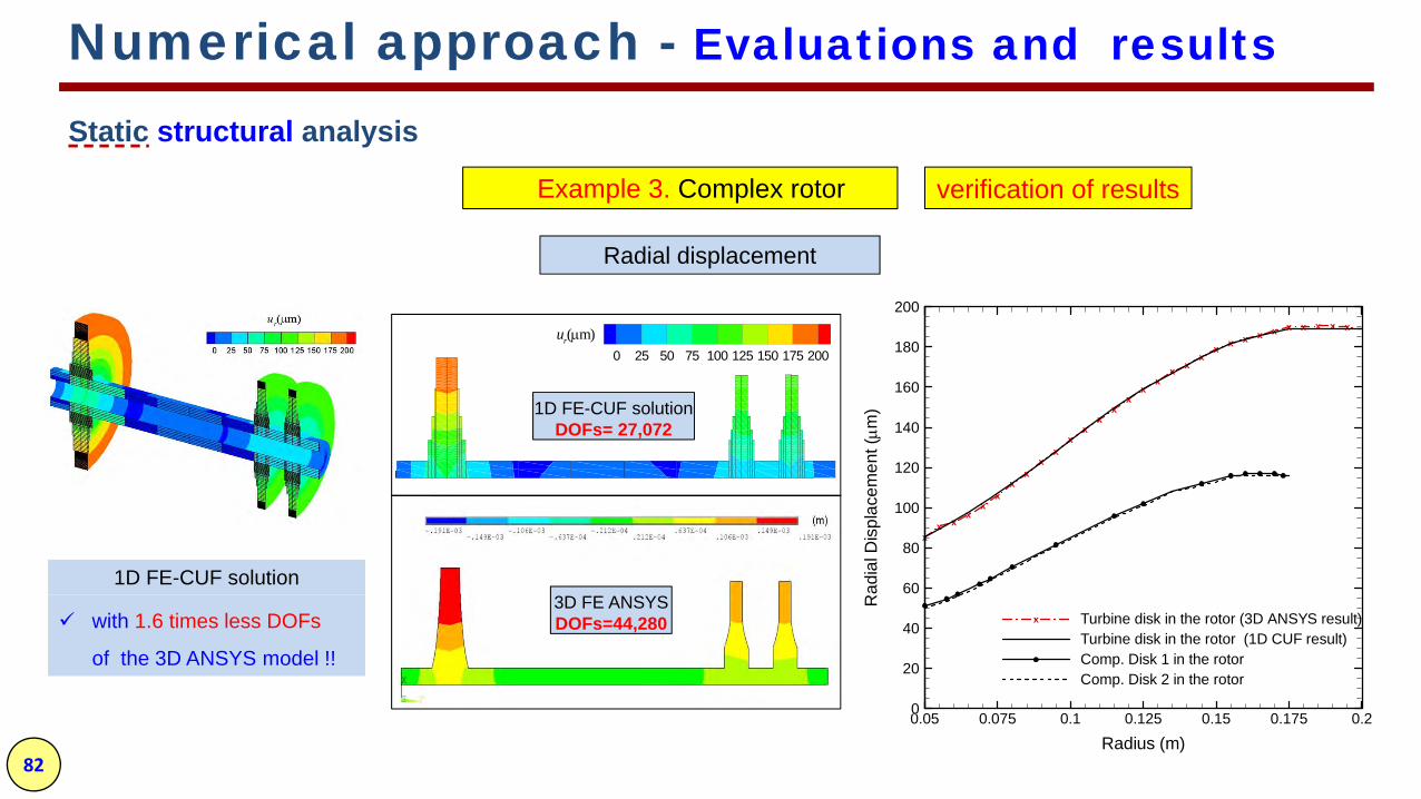
Numerical approach - Evaluations and results
Static structural analysis
Example 3. Complex rotor verification of results
0 25 50 75 100 125 150 175 200ur(m)
1D FE-CUF solutionDOFs= 27,072
3D FE ANSYSDOFs=44,280
xx x
xx
xx
xx
xx
xx
xx
xx
x xx
x x x x x x x x x x
Radius (m)
Rad
ialD
ispl
acem
ent(m
)
0.05 0.075 0.1 0.125 0.15 0.175 0.20
20
40
60
80
100
120
140
160
180
200
Turbine disk in the rotor (3D ANSYS result)Turbine disk in the rotor (1D CUF result)Comp. Disk 1 in the rotorComp. Disk 2 in the rotor
x
1D FE-CUF solution
Radial displacement
with 1.6 times less DOFs
of the 3D ANSYS model !!

83
Radius (m)
Stre
ss(M
Pa)
0.05 0.075 0.1 0.125 0.15 0.175 0.20
50
100
150
200
250
300
350
400
450
500
550
Turbine disk in the rotorSingle Turbine disk with rigid hub
rr
rr
Numerical approach - Evaluations and results
50 100 150 200 250 300 350 400 450 500 550 600 650 700rr(MPa)
50 100 150 200 250 300 350 400 450 500 550(MPa)
Static structural analysis
Example 3. Complex rotor verification of results
Radial and circumferential stresses
Circumferential stress
Radial stress

1. Introduction to rotating disk2. Fundamentals of Linear Thermoelasticity3. Literature review & present work4. Analytical approach5. Numerical approach Motivation Development of method Evaluations and results
o Static structural analysisExample 1. Rotating variable thickness diskExample 2. Rotating variable thickness disk subjected thermal loadExample 3. Complex rotor
o Static structural-thermal analysis – Example 4. simple beam
o Quasi-static structural-thermal analysis – Example 5. simple beam
o Dynamic coupled structural-thermal analysis
Example 6. Constant thickness disk made of isotropic homogeneous materialsExample 7. Constant thickness disk made of isotropic FGMs Example 8. variable thickness disk made of isotropic FGMs
6. Conclusion
Outlines

85
Static structural-thermal analysis
Numerical approach - Evaluations and results
Example 4. simple beam
Lagrange elements over the cross-section
discretizing along the axis
1D FE-CUF modeling
86
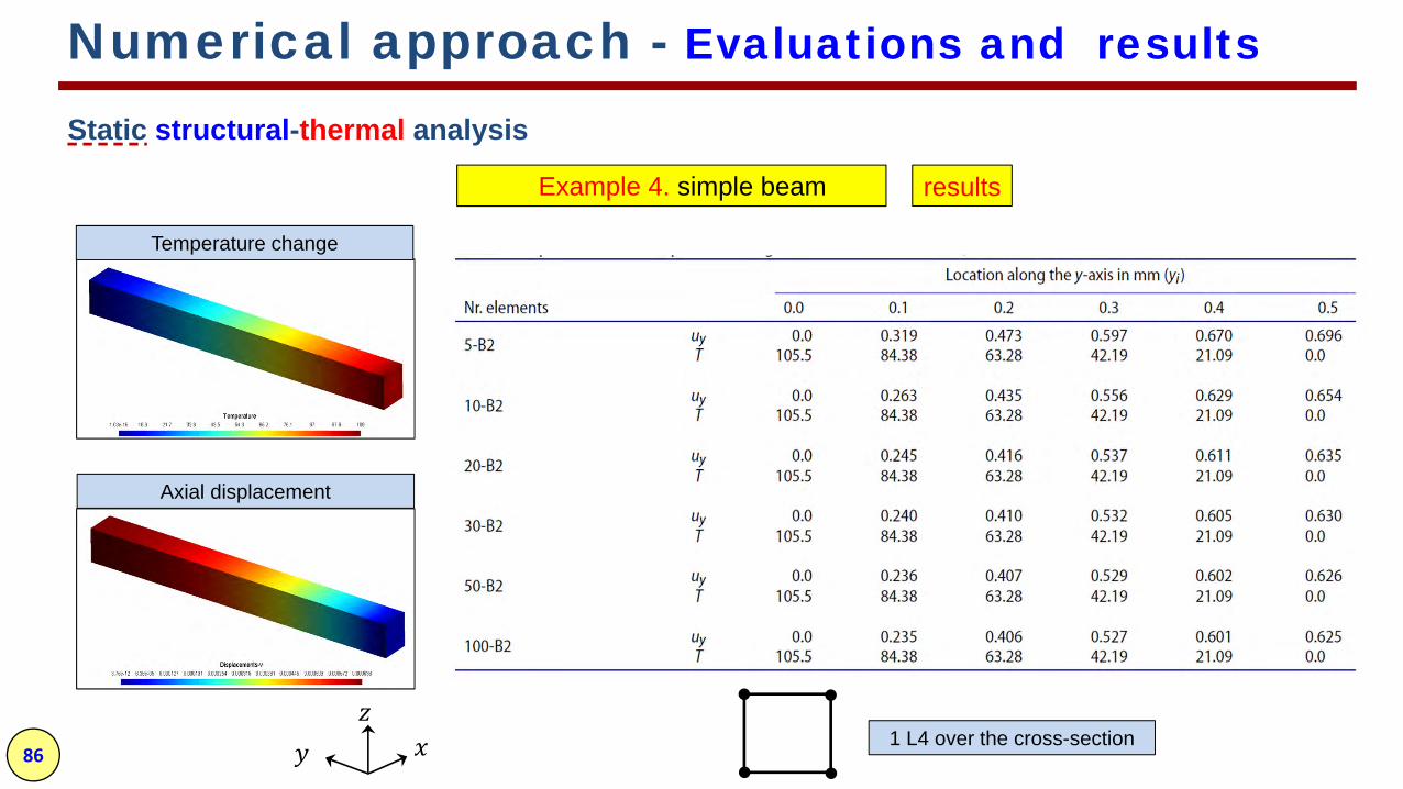
Numerical approach - Evaluations and results
Static structural-thermal analysis
Example 4. simple beam
Temperature change
Axial displacement
results
1 L4 over the cross-section

87
Numerical approach - Evaluations and results
Static structural-thermal analysis
Example 4. simple beam results
1 L9 over the cross-section
1 L16 over the cross-section
88
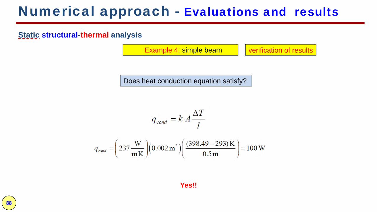
Yes!!
Does heat conduction equation satisfy?
Numerical approach - Evaluations and results
Static structural-thermal analysis
Example 4. simple beam verification of results
89
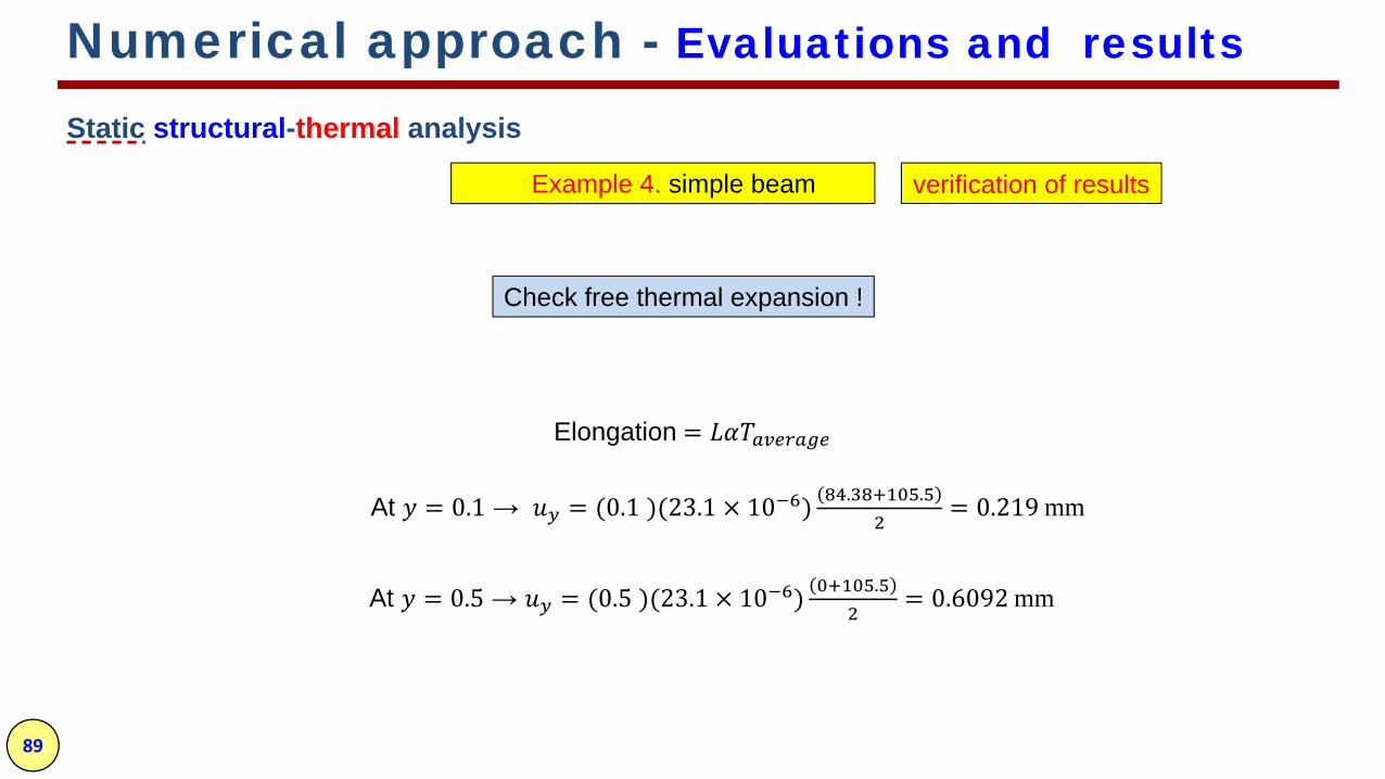
At = 0.1→ = (0.1 )(23.1 × 10 ) . . = 0.219 mm
At = 0.5→ = (0.5 )(23.1 × 10 ) . = 0.6092 mm
Elongation =
Numerical approach - Evaluations and results
Static structural-thermal analysis
Example 4. simple beam verification of results
Check free thermal expansion !

1. Introduction to rotating disk2. Fundamentals of Linear Thermoelasticity3. Literature review & present work4. Analytical approach5. Numerical approach Motivation Development of method Evaluations and results
o Static structural analysisExample 1. Rotating variable thickness diskExample 2. Rotating variable thickness disk subjected thermal loadExample 3. Complex rotor
o Static structural-thermal analysis – Example 4. simple beam
o Quasi-static structural-thermal analysis – Example 5. simple beam
o Dynamic coupled structural-thermal analysis
Example 6. Constant thickness disk made of isotropic homogeneous materialsExample 7. Constant thickness disk made of isotropic FGMs Example 8. variable thickness disk made of isotropic FGMs
6. Conclusion
Outlines

91
Numerical approach - Evaluations and results
Example 5. simple beam
Quasi-static structural-thermal analysis
Transient heat flux (thermal load)

92
Numerical approach - Evaluations and results
Example 5. simple beam
Quasi-static structural-thermal analysis
results
Temperature changeAxial displacement
10B4/1L4 model
Axial displacement Temperature change

93
1. Introduction to rotating disk2. Fundamentals of Linear Thermoelasticity3. Literature review & present work4. Analytical approach5. Numerical approach Motivation Development of method Evaluations and results
o Static structural analysisExample 1. Rotating variable thickness diskExample 2. Rotating variable thickness disk subjected thermal loadExample 3. Complex rotor
o Static structural-thermal analysis – Example 4. simple beam
o Quasi-static structural-thermal analysis – Example 5. simple beam
o Dynamic coupled structural-thermal analysisExample 6. Constant thickness disk made of isotropic homogeneous materialsExample 7. Constant thickness disk made of isotropic FGMs Example 8. variable thickness disk made of isotropic FGMs
6. Conclusion
Outlines

94
Lame’constant λ 40.4GPaLame’ constant μ 27GPacoefficient of linear thermal expansion (α) 23 × 10 Kdensity (ρ) 2707kg/mthermal conductivity (κ) 204W/m ∙ Kspecific heat (c) 903J/kg ∙ K
Material properties
Dynamic coupled structural-thermal analysis
Numerical approach - Evaluations and results
Example 6. Constant thickness disk made of isotropic homogeneous materials
geometry= 1= 2Thickness = 0.1
Boundary conditions
= → − = ( )= 0 = → = 0= 0
where ( ) = 0 01 0

95
Numerical approach - Evaluations and results
Dynamic coupled structural-thermal analysis
Example 6. Constant thickness disk made of isotropic homogeneous materials 1D FE-CUF modeling
DOFDiscretizingModel corss sectionsAlong the axis1680(6 × 30)L41 B2(1)25201 B3(2)33601 B4(3)
16803 × 15 L91 B2
(4) 2 × 10 L16(5)37446 × 18 L9(6)
Lagrange mesh over the cross-section with the largest radius
discretizing along the axis Different 1D FE-CUF models for the constant thickness disk

96
Nondimensional Time (t)
Non
dim
ensio
nalR
adia
lDisp
lace
men
t(u)
0 2 4 6 8 10 12 14
-0.2
-0.1
0
0.1
0.2
0.3
0.4
0.5
0.6
0.7
0.8
0.9
1
Exact Solution (Entezari, 2016)Axisymetric FE (Bagri, 2004)CUF: 1 B2/(618) L9
t0 =0.64, C =0.02, r =1.5
Nondimensional Time (t)
Non
dim
ensio
nalT
empe
ratu
re(T
)
0 2 4 6 8 10 12 140
0.05
0.1
0.15
0.2
0.25
0.3
0.35
0.4
0.45
0.5
Exact Solution (Entezari, 2016)Axisymetric FE (Bagri, 2004)CUF: 1 B2/(618) L9
t0 =0.64, C =0.02, r =1.5
Numerical approach - Evaluations and results
Dynamic coupled structural-thermal analysis
Example 6. Constant thickness disk made of isotropic homogeneous materials verification of results
Based on the LS theoryof thermoelasticity
Time history of solution at mid-radius of the disk.
Temperature change Radial displacement
1B2 / 6 × 18 L9

97
Numerical approach - Evaluations and results
Dynamic coupled structural-thermal analysis
Example 6. Constant thickness disk made of isotropic homogeneous materials verification of results
Based on the LS theoryof thermoelasticity
Time history of solution at mid-radius of the disk.
1B2 / 6 × 18 L9 Nondimensional Time (t)
Non
dim
ensio
nalT
ange
ntia
lStre
ss(
)
0 2 4 6 8 10 12 14
-0.6
-0.4
-0.2
0
0.2
0.4
0.6
0.8
Exact Solution (Entezari, 2016)CUF: 1 B2/(618) L9
t0 =0.64, C =0.02, r =1.5
Nondimensional Time (t)
Non
dim
ensio
nalR
adia
lStre
ss(
rr)
0 2 4 6 8 10 12 14
-0.8
-0.6
-0.4
-0.2
0
0.2
0.4
0.6
0.8
1
Exact Solution (Entezari, 2016)CUF: 1 B2/(618) L9
t0 =0.64, C =0.02, r =1.5
Circumferential stressRadial stress

1. Introduction to rotating disk2. Fundamentals of Linear Thermoelasticity3. Literature review & present work4. Analytical approach5. Numerical approach Motivation Development of method Evaluations and results
o Static structural analysisExample 1. Rotating variable thickness diskExample 2. Rotating variable thickness disk subjected thermal loadExample 3. Complex rotor
o Static structural-thermal analysis – Example 4. simple beam
o Quasi-static structural-thermal analysis – Example 5. simple beam
o Dynamic coupled structural-thermal analysisExample 6. Constant thickness disk made of isotropic homogeneous materialsExample 7. Constant thickness disk made of isotropic FGM Example 8. variable thickness disk made of isotropic FGMs
6. Conclusion
Outlines

99
Metal: Aluminum Ceramic: AluminaLame’constant λ 40.4 GPa 219.2 GPashear modulus μ 27.0 GPa 146.2 GPadensity (ρ) 2707 kg/m3 3800 kg/m3
coefficient of linear thermal expansion (α) 23.0106 K1 7.4106 K1
thermal conductivity (κ) 204 W/mK 28.0 W/mKspecific heat (c) 903 J/kgK 760 J/kgKdimensionless relaxation time ( ) 0.64 1.5625
Numerical approach - Evaluations and results
Dynamic coupled structural-thermal analysis
Example 7. Constant thickness disk made of isotropic FGM
Material properties Metal-Ceramic FGM
geometry= 1= 2Thickness = 0.1
Geometry and material
effective properties
P=VmPm +Vc Pc =Vm (Pm−Pc)+Pc
metal volume fraction
Vm = − −

100
z
xFixed
Free
y
z
Adiabatic
T(t)Non-dimensional form
= 293 K, =0.01
at = 0 → = = = = 0
Numerical approach - Evaluations and results
Dynamic coupled structural-thermal analysis
Example 7. Constant thickness disk made of isotropic FGM Operational, boundary & initial conditions
( ) = (1 − [1 + 100 mm] m m⁄ )
( ) = 1 − (1 + 100 )
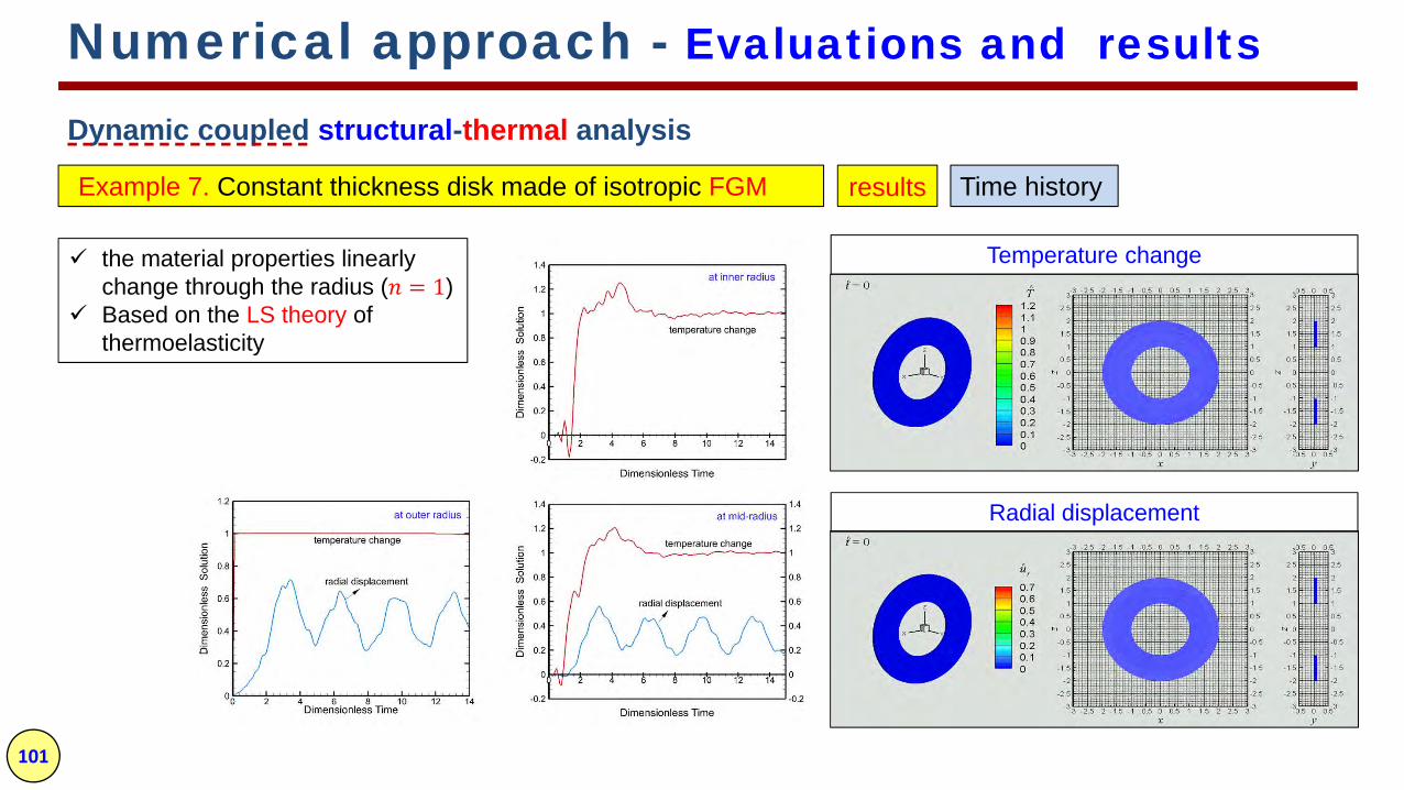
101
Time history
Numerical approach - Evaluations and results
Dynamic coupled structural-thermal analysis
Example 7. Constant thickness disk made of isotropic FGM results
the material properties linearly change through the radius ( = 1)
Based on the LS theory of thermoelasticity
Temperature change
Radial displacement

102
Axial deformation
Numerical approach - Evaluations and results
Deformations of disk profile
Dynamic coupled structural-thermal analysis
Example 7. Constant thickness disk made of isotropic FGM results
Radial displacement radial deformation
Time history
the material properties linearly change through the radius ( = 1)
Based on the LS theory of thermoelasticity

103
Numerical approach - Evaluations and results
Dynamic coupled structural-thermal analysis
Example 7. Constant thickness disk made of isotropic FGM results Speed range of the thermal wave
the material properties linearly change through the radius ( = 1)
Based on the LS theory of thermoelasticity

104
Numerical approach - Evaluations and results
Dynamic coupled structural-thermal analysis
Example 7. Constant thickness disk made of isotropic FGM results Speed range of the thermal wave
the material properties linearly change through the radius ( = 1)
Based on the LS theory of thermoelasticity
wave reflection ≃ 1/1.5 = 0.6

105
1 1.25⁄ 1 0.27⁄0.8 3.7
Numerical approach - Evaluations and results
Dynamic coupled structural-thermal analysis
Example 7. Constant thickness disk made of isotropic FGM results
c = c m⁄ 1 c⁄ = 0.27m = 1 m⁄ = 1.25
Thermal wave propagation
m, , − m m
+ − , + ,+ + = 0Non-dimensional form of energy equation
the material properties linearly change through the radius ( = 1)
Based on the LS theory of thermoelasticity
Speed range of the thermal wave 0.27 ,FGM 1.25wave reflection ≃ 1/1.5 = 0.6

106
Numerical approach - Evaluations and results
Dynamic coupled structural-thermal analysis
Example 7. Constant thickness disk made of isotropic FGM results Elastic wave propagation
the material properties linearly change through the radius ( = 1)
Based on the LS theory of thermoelasticity
wave reflection

107
Numerical approach - Evaluations and results
Dynamic coupled structural-thermal analysis
Example 7. Constant thickness disk made of isotropic FGM results Elastic wave propagation
the material properties linearly change through the radius ( = 1)
Based on the LS theory of thermoelasticity
wave reflectionNon-dimensional form of equation of motion
m + 2 m, + +
m + 2 m, + 1
m + 2 m, ,+ 1
m + 2 m, ( , + , ) −
m− 1
m, + , + = 0 c = 1.96
m = 1 →1 FGM 1.96 0.51 1Speed range of elastic wave

108
X
X
X
X
X
X
X
X
X
X
XX X
X XX
X X XX X X X X X X X X X X X X X X X X X
Nondimensional time(t)
Non
dim
ensio
nalt
empe
ratu
rech
ange
(T)
0 2 4 6 8 10 12 14-0.2
0
0.2
0.4
0.6
0.8
1
1.2
1.4
n = 0n = 1n = 2n = 5X
at mid radius
X X X X X X X X XX
X X XX X X
XX X
XX X
XX X
XX
X XX
X XX
X X XX X
Nondimensional time(t)N
ondi
men
siona
lrad
iald
ispla
cem
ent(
u r)0 2 4 6 8 10 12 14
-0.4
-0.2
0
0.2
0.4
0.6
0.8
1
1.2
1.4
1.6
n = 0n = 1n = 2n = 5X
at mid radius
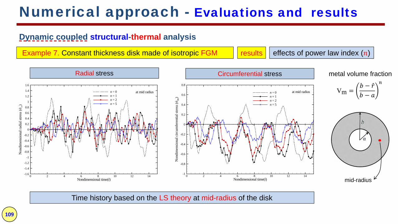
Time history based on the LS theory at mid-radius of the disk
Numerical approach - Evaluations and results
Dynamic coupled structural-thermal analysis
Example 7. Constant thickness disk made of isotropic FGM results
Temperature change Radial displacement
mid-radius
effects of power law index ( )
metal volume fraction
Vm = − −
109
Time history based on the LS theory at mid-radius of the disk
Numerical approach - Evaluations and results
Dynamic coupled structural-thermal analysis
Example 7. Constant thickness disk made of isotropic FGM results
Radial stress Circumferential stress
mid-radius
effects of power law index ( )
metal volume fraction
Vm = − −X X
XX
XX
X XX
XX X
XX
X X
X
XX
X
X
X
X
X X
X
X
X
X
X XX
X
XX
XX X
X
X XX
XX X
XX
X
XX
X
X
XX
XX
X
X
XX
X X
X
X
X XX X
XX
XX
XX
X
Nondimensional time(t)
Non
dim
ensio
nalr
adia
lstre
ss(
rr)
0 2 4 6 8 10 12 14-1.6
-1.4
-1.2
-1
-0.8
-0.6
-0.4
-0.2
0
0.2
0.4
0.6
0.8
1
1.2
1.4
1.6
n = 0n = 1n = 2n = 5X
at mid radius
XX
XX
XX
X XX
X
X X XX
X
X
X
XX
XX
XX
X
X X
X
XX X
X X
X
X X X
X
X
X
XX
XX
XX
XX X
X XX
X
XX X X X
X
XX
X X X
X
XX
X XX
X
X
XX X
X
Nondimensional time(t)N
ondi
men
siona
lcirc
umfe
rent
ials
tress
(
)0 2 4 6 8 10 12 14
-1
-0.8
-0.6
-0.4
-0.2
0
0.2
0.4
0.6
0.8
n = 0n = 1n = 2n = 5X
at mid radius

110
Time history based on the LS theory at mid-radius of the disk (n =1)
Numerical approach - Evaluations and results
Dynamic coupled structural-thermal analysis
Example 7. Constant thickness disk made of isotropic FGM results
mid-radius
effects of reference temperature ( )
X
X
X
X X
XX
X XX
XX X
XX X X
X X X X X X X X X X X X X X X X X X X X
Nondimensional time(t)
Non
dim
ensio
nalt
empe
ratu
rech
ange
(T)
0 2 4 6 8 10 12 14-0.2
0
0.2
0.4
0.6
0.8
1
1.2
1.4
T0 = 0T0 = 293T0 = 800
X
at mid radius
X X X XX X X
XX
X
X
X
X
X
X
X
X
X
XX
X
X
X
X
X X X
X
X
X
X X X
XX
X
X
X
X X
XX
X
X
X
XX
X
X XX
X
XX
X
X
XX
X
X X
X
X
X
XX
X XX
X
X
X
XX
X
Nondimensional time(t)N
ondi
men
siona
lrad
iald
ispla
cem
ent(
u r)0 2 4 6 8 10 12 14
0
0.1
0.2
0.3
0.4
0.5
0.6
T0 = 0T0 = 293T0 = 800
X
at mid radius
Radial displacementTemperature change = mm m( m + m)
coupling parameter

111
Time history based on the LS theory at mid-radius of the disk (n =1)
Numerical approach - Evaluations and results
Dynamic coupled structural-thermal analysis
Example 7. Constant thickness disk made of isotropic FGM results
mid-radius
effects of reference temperature ( )
= mm m( m + m)
coupling parameter
X XX X X X
XX
X
X XX
X
X X
X
X
X
X
X
X
X
X
X
X
X
XX
X
X
X X
X
X
X
X
X
XX
X
X
X
X
X
X
X
X X
X
X
X
X
X
X
X
X
X
X
X
X
X
X
X
X
X
X
XX
X
XX
X
X
X
X
Nondimensional time(t)
Non
dim
ensio
nalr
adia
lstre
ss(
rr)
0 2 4 6 8 10 12 14-1
-0.8
-0.6
-0.4
-0.2
0
0.2
0.4
0.6
0.8
1
1.2
1.4
1.6
T0 = 0T0 = 293T0 = 800
X at mid radius
X XX
XX
X
X X X X
X
X
X
X
X
X
X
XX
X
X
X
X
X
X
X
X
X
X
X
X X
X
X
X
X
X
X
X
X XX
X
X
X
X
X
X X
X
X X
X
X
XX
X
X
X
X
X
XX X X
X
X X
X X
XX
X
X
X
Nondimensional time(t)N
ondi
men
siona
lcirc
umfe
rent
ials
tress
(
)0 2 4 6 8 10 12 14
-1
-0.8
-0.6
-0.4
-0.2
0
0.2
0.4
0.6
0.8
T0 = 0T0 = 293T0 = 800
X at mid radius
Radial stress Circumferential stress

112
1. Introduction to rotating disk2. Fundamentals of Linear Thermoelasticity3. Literature review & present work4. Analytical approach5. Numerical approach Motivation Development of method Evaluations and results
o Static structural analysisExample 1. Rotating variable thickness diskExample 2. Rotating variable thickness disk subjected thermal loadExample 3. Complex rotor
o Static structural-thermal analysis – Example 4. simple beam
o Quasi-static structural-thermal analysis – Example 5. simple beam
o Dynamic coupled structural-thermal analysisExample 6. Constant thickness disk made of isotropic homogeneous materialsExample 7. Constant thickness disk made of isotropic FGMExample 8. variable thickness disk made of isotropic FGM
6. Conclusion
Outlines

113
0.3
2
0.5
0.6
h = 0.42 r-0.5
r
Numerical approach - Evaluations and results
Dynamic coupled structural-thermal analysis
Example 8. variable thickness disk made of isotropic FGM Geometry and material
Metal: Aluminum Ceramic: AluminaLame’constant λ 40.4 GPa 219.2 GPashear modulus μ 27.0 GPa 146.2 GPadensity (ρ) 2707 kg/m3 3800 kg/m3
coefficient of linear thermal expansion (α) 23.0106 K1 7.4106 K1
thermal conductivity (κ) 204 W/mK 28.0 W/mKspecific heat (c) 903 J/kgK 760 J/kgKdimensionless relaxation time ( ) 0.64 1.5625
Material properties Metal-Ceramic FGM
geometry = = 0.5 = = 2ℎ = 0.6ℎ = 0.3effective properties
P=VmPm +Vc Pc =Vm (Pm−Pc)+Pc
metal volume fraction
Vm = − −

114
= 293 K, =0.05
at = 0 → = = = = 0
Numerical approach - Evaluations and results
Dynamic coupled structural-thermal analysis
Operational, boundary & initial conditionsExample 8. variable thickness disk made of isotropic FGM
Non-dimensional form
( ) = (1 − m⁄ )
( ) = 1 −

115
Numerical approach - Evaluations and results
Dynamic coupled structural-thermal analysis
Example 8. variable thickness disk made of isotropic FGM Results for = 0
Nondimensional time
Non
dim
ensi
onal
tem
pera
ture
chan
ge
0 2 4 6 8 10 12 14
-0.2
0
0.2
0.4
0.6
0.8
1
Classic theoryLS theory
Temperature change
Nondimensional time
Non
dim
ensi
onal
radi
alst
ress
0 2 4 6 8 10 12 14
-1
-0.8
-0.6
-0.4
-0.2
0
0.2
0.4
0.6
0.8
1
1.2
1.4
Classic theoryLS theory
Radial stress
Nondimensional time
Non
dim
ensi
onal
von
mis
eseq
uiva
lent
stre
ss
0 2 4 6 8 10 12 140
0.2
0.4
0.6
0.8
1
Classic theoryLS theory
Von mises stress
Nondimensional time
Non
dim
ensi
onal
circ
umfe
rent
ials
tress
0 2 4 6 8 10 12 14
-1
-0.8
-0.6
-0.4
-0.2
0
0.2
0.4
0.6
0.8
1
1.2
1.4
Classic theoryLS theory
Circumferential stress
Nondimensional time
Non
dim
ensi
onal
radi
aldi
spla
cem
ent
0 2 4 6 8 10 12 14
-0.2
0
0.2
0.4
0.6
0.8
1
Classic theoryLS theory
Radial displacement
116
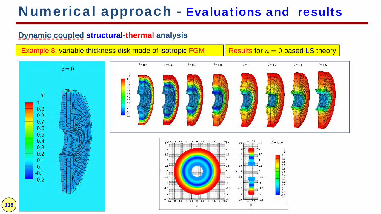
Numerical approach - Evaluations and results
Dynamic coupled structural-thermal analysis
Example 8. variable thickness disk made of isotropic FGM Results for = 0 based LS theory

117
Numerical approach - Evaluations and results
Dynamic coupled structural-thermal analysis
Example 8. variable thickness disk made of isotropic FGM
Rad
iald
ispl
acem
ent
Axi
al d
ispl
acem
ent
Results for = 0 based LS theory

118
Outlines
1. Introduction to rotating disks
2. Fundamentals of Linear Thermoelasticity
3. Literature review & present work
4. Analytical approach
5. Numerical approach
6. Conclusion

119
Some results obtained from coupled thermoelasticity solution
Conclusion - Summary of results
Transient deformations and stresses may be higher than those of a steady-state condition.
Time history of temperature is damped faster than time history of displacements.
Deformations and stresses oscillate along the time in a harmonic form.
Under the propagating longitudinal elastic waves along the radius, thickness of the disk also expands and
contracts, due to the Poisson effect.
When the coupling parameter takes a greater value, the amplitudes of oscillations of temperature
increase.
Lord–Shulman generalized coupled thermoelasticity predicts larger temperature and stresses compared
to the classical theories.
A functionally graded disk may be used as thermal barrier to reduce the thermal shock effects.

120
Conclusion - Summary of results
Some general points on the 1D FE-CUF modeling of disks The 1D FE method refined by the CUF can be effectively employed to analyze disks reduce the
computational cost of 3D FE analysis without affecting the accuracy.
the models provides a unified formulation that can easily consider different higher-order theories wherelarge bending loads are involved in the problem.
Increasing 1D elements along the axis of disks may not have significant effect on accuracy of resultsand only leads to more DOFs.
A proper distribution of the Lagrange elements and type of element used over the cross sections maylead to a reduction in computational costs and the convergence of results.
Making use of higher-order Lagrange elements (like L9 and L16) can reduce DOFs, while preservingthe accuracy.
increase of number of elements along the radial direction, compared to circumferential direction, ismore effective in improving the results.

121
Conclusion - Future works
Nonlinear thermoelasticity problems
Dynamic analysis of rotors subjected to transient thermal pre-stresses.
Study of thermoelastic damping effect on dynamic behaviors of rotors.
It is of interests to extend the study to

122
1. Entezari A, Filippi M, Carrera E., Kouchakzadeh M A, 3D Dynamic Coupled Thermoelastic Solution For ConstantThickness Disks Using Refined 1D Finite Element Models. European Journal of Mechanics - A/Solids. (Underreview).
2. Entezari A, Filippi M, Carrera E. Unified finite element approach for generalized coupled thermoelastic analysisof 3D beam-type structures, part 1: Equations and formulation. Journal of Thermal Stresses. 2017:1-16.
3. Filippi M, Entezari A, Carrera E. Unified finite element approach for generalized coupled thermoelastic analysisof 3D beam-type structures, part 2: Numerical evaluations. Journal of Thermal Stresses. 2017:1-15.
4. Entezari A, Filippi M, Carrera E. On dynamic analysis of variable thickness disks and complex rotors subjectedto thermal and mechanical prestresses. Journal of Sound and Vibration. 2017;405:68-85.
5. Kouchakzadeh MA, Entezari A, Carrera E. Exact Solutions for Dynamic and Quasi-Static ThermoelasticityProblems in Rotating Disks. Aerotecnica Missili & Spazio. 2016;95:3-12.
6. Entezari A, Kouchakzadeh MA, Carrera E, Filippi M. A refined finite element method for stress analysis of rotorsand rotating disks with variable thickness. Acta Mechanica. 2016:1-20.
7. Entezari A, Kouchakzadeh MA. Analytical solution of generalized coupled thermoelasticity problem in a rotatingdisk subjected to thermal and mechanical shock loads. Journal of Thermal Stresses. 2016:1-22.
8. Carrera E, Entezari A, Filippi M, Kouchakzadeh MA. 3D thermoelastic analysis of rotating disks having arbitraryprofile based on a variable kinematic 1D finite element method. Journal of Thermal Stresses. 2016:1-16.
9. Kouchakzadeh MA, Entezari A. Analytical Solution of Classic Coupled Thermoelasticity Problem in a RotatingDisk. Journal of Thermal Stresses. 2015;38:1269-91.
Publications in international Journals

Acknowledgements
Professor M. A. Kouchakzadeh and Erasmo Carrera, my supervisors
Dr. Matteo Filippi, my advisor and colleague in Italy.
Professors Hassan Haddadpour and Ali Hosseini Kordkheili, my Iranian committee members
Professors Maria Cinefra and Elvio Bonisoli, my Italian committee members
Doctoral Dissertation on
Solution of Coupled Thermoelasticity Problem In Rotating Disks
byAyoob Entezari
26 September, 2017
Supervisors:Prof. M. A. Kouchakzadeh¹ and Prof. Erasmo Carrera²
¹Sharif University of TechnologyDepartment of Aerospace Engineering, Tehran, Iran
²Polytechnic University of Turin, Department of Mechanical and Aerospace Engineering, Italy
²MUL2 research group, Polytechnic University of Turin, Italy
Cotutelle Doctoral Program
Thank you for your attention!