Embed Size (px)
DESCRIPTION
Probability and statistics solution manual
Citation preview
Continuous Random Variables 75
CHAPTER 5 ………………………………………………………….. Continuous Random Variables 5.2 a. We know that
1
0
(2 ) 1c y dy− =∫
1
0
(2 ) 1c cy dy⇒ − =∫
12
0
2 2 (0 0) 12 2
cy ccy c⎤ ⎛ ⎞⇒ − = − − − =⎥ ⎜ ⎟
⎝ ⎠⎦
3 212 3c c⇒ = ⇒ =
b. 2
0 0
2 4 1( ) ( ) (2 )3 3 3
yy y
F y f t dt t dt t t−∞
⎤= = − = − ⎥
⎥⎦∫ ∫
= 2 24 1 4 1(0 0)3 3 3 3
y y y y⎛ ⎞− − − = −⎜ ⎟⎝ ⎠
= 21 (4 )3
y y−
c. 21(.4) 4(.4) (.4) .483
F ⎡ ⎤= − =⎣ ⎦
d. 6
.1
2(.1 .6) (2 )3
P y y dy≤ ≤ = −∫
= .6
2
.1
4 13 3
y y ⎤⎛ ⎞−⎜ ⎟⎥⎝ ⎠⎦
= 2 24 1 4 1(.6) (.6) (.1) (.1)3 3 3 3⎡ ⎤ ⎡ ⎤− − −⎢ ⎥ ⎢ ⎥⎣ ⎦ ⎣ ⎦
= .67 − .13 = .55
76 Chapter 5
5.4 a. We know
0
/ 2 / 2
0
1 1 1y ye dy e dyc c
∞−
−∞
⎛ ⎞ ⎛ ⎞+ =⎜ ⎟ ⎜ ⎟⎝ ⎠ ⎝ ⎠∫ ∫
0
/ 2 / 2
0
2 2 1y ye ec c
∞−
−∞
−⎤ ⎤⇒ + =⎥ ⎥⎦ ⎦
2 20 0 1c c
−⎛ ⎞ ⎛ ⎞⇒ − + − =⎜ ⎟ ⎜ ⎟⎝ ⎠ ⎝ ⎠
2 2 41 1 4cc c c
⇒ + = ⇒ = ⇒ =
b. If / 210 : ( ) ( )4
y yty F y f t dt e dt
−∞ −∞
⎛ ⎞< = = ⎜ ⎟⎝ ⎠∫ ∫
= / 2 / 2 / 22 2 104 4 2
yt y ye e e
−∞
⎤ = − =⎥⎦
If / 2
0
1 10 : ( )2 4
yty F y e dt−⎛ ⎞≥ = + ⎜ ⎟
⎝ ⎠∫
= / 2 / 2 / 2
0
1 2 1 1 1 112 4 2 2 2 2
yt y ye e e− − −− − −⎤ ⎛ ⎞+ = + − = −⎜ ⎟⎥⎦ ⎝ ⎠
/ 2
/ 2
1 02( )
11 02
y
y
e yF t
e y−
⎧ <⎪⎪= ⎨⎪ − ≥⎪⎩
c. 1/ 21(1) 1 1 .303 .6972
F e−= − = − =
d. / 2 / 2 .5/ 2
.5 .5
1 1 1( .5) 04 2 2
y yP y e dy e e∞∞
− − −⎤− −⎛ ⎞> = = = −⎥ ⎜ ⎟
⎝ ⎠⎥⎦∫
= .5/ 21 .38942
e− =
Continuous Random Variables 77
5.6 a. 2 2 2
0 0
( ) ( ) / 2 04 4 4
yy y t y yF y f t dt t dtθ−
⎤= = = = − =⎥
⎥⎦∫ ∫
b. 2
( ) 14yF y = −
Let x = 1 and y = 12
Then,
( )233 2( ) 1 .43752 4
F x y F
⎛ ⎞⎜ ⎟⎛ ⎞ ⎝ ⎠+ = = − =⎜ ⎟
⎝ ⎠
( )21( ) (1) 1 .75
4F x F= = − =
211 2( ) 1 .93752 4
F y F
⎛ ⎞⎜ ⎟⎛ ⎞ ⎝ ⎠= = − =⎜ ⎟
⎝ ⎠
( ) ( ) .75(.9375) .703125F x F y = =
Since ( ) ( ) ( ),F x y F x F y+ ≤ the “life” distribution is NBU.
5.8 a. Show ( ) 1f y dy∞
−∞
=∫
2 2( ) ( )c
c
c y c ydy dyc c
μ μ
μ μ
μ μ+
−
− + + −+∫ ∫
= 2 2
2 21 1( ) ( )
2 2
c
c
y yc y c yc c
μ μ
μ μ
μ μ+
−
⎤ ⎤⎛ ⎞ ⎛ ⎞− + + + −⎥ ⎥⎜ ⎟ ⎜ ⎟
⎥ ⎥⎝ ⎠ ⎝ ⎠⎦ ⎦
= 2 2
21 ( )( ) ( )( )
2 2cc c c
cμ μμ μ μ μ
⎧ ⎫⎛ ⎞−⎪ ⎪− + − − − +⎨ ⎬⎜ ⎟⎪ ⎪⎝ ⎠⎩ ⎭
2 2 21 ( )( )( ) ( )
2 2cc c c
cμ μμ μ μ μ
⎧ ⎫⎛ ⎞+⎪ ⎪+ + + − − + −⎨ ⎬⎜ ⎟⎪ ⎪⎝ ⎠⎩ ⎭
= 2 2 2
2 2 22
1 22 2 2
cc c c cc
μ μμ μ μ μ μ⎧ ⎫
− + + − + + − + −⎨ ⎬⎩ ⎭
+ 2 2 2
2 2 22
1 22 2 2
cc c c cc
μ μμ μ μ μ μ⎧ ⎫
+ + − − − − − +⎨ ⎬⎩ ⎭
= 2 2
2 21 1 1 1 1
2 2 2 2c c
c c⎛ ⎞ ⎛ ⎞
+ = + =⎜ ⎟ ⎜ ⎟⎝ ⎠ ⎝ ⎠
78 Chapter 5
b. 2 2
2 2( ) ( )( )
c
c
c y y c y yE y dy dyc c
μ μ
μ μ
μ μ+
−
− + + −= +∫ ∫
= 2 3 2 3
2 21 ( ) 1 ( )
2 3 2 3
c
c
c y y c y yc c
μ μ
μ μ
μ μ+
−
⎤ ⎤⎛ ⎞ ⎛ ⎞− ++ + −⎥ ⎥⎜ ⎟ ⎜ ⎟
⎥ ⎥⎝ ⎠ ⎝ ⎠⎦ ⎦
= 2 3 2 3
21 ( ) ( )( ) ( )
2 3 2 3c c c c
cμ μ μ μ μ μ⎧ ⎫⎛ ⎞− − − −⎪ ⎪+ − +⎨ ⎬⎜ ⎟
⎪ ⎪⎝ ⎠⎩ ⎭
+ 2 3 2 3
21 ( )( ) ( ) ( )
2 3 2 3c c c c
cμ μ μ μ μ μ⎧ ⎫⎛ ⎞+ + + +⎪ ⎪− − −⎨ ⎬⎜ ⎟
⎪ ⎪⎝ ⎠⎩ ⎭
= 2 3 3 3 2 2 3 3 2 2 3
21 3 3 3 3
2 2 3 2 3c c c c c c c
cμ μ μ μ μ μ μ μ μ⎧ ⎫⎛ ⎞− + − − + −⎪ ⎪− + − +⎨ ⎬⎜ ⎟
⎪ ⎪⎝ ⎠⎩ ⎭
+ 3 2 2 3 3 2 2 3 2 3 3
21 3 3 3 3
2 3 2 2 3c c c c c c c
cμ μ μ μ μ μ μ μ μ⎧ ⎫⎛ ⎞+ + + + + −⎪ ⎪− − + +⎨ ⎬⎜ ⎟
⎪ ⎪⎝ ⎠⎩ ⎭
= ( ) ( )2 3 3 2 2 3 3 3 2 2 32
1 1 13 3 3 32 3
c c c c c c cc
μ μ μ μ μ μ μ μ μ⎧ ⎫− − + − + + − + − +⎨ ⎬⎩ ⎭
+ ( ) ( )3 2 2 3 2 3 3 2 2 32
1 1 13 3 3 32 3
c c c c c c cc
μ μ μ μ μ μ μ μ μ⎧ ⎫+ + + − + + − − − − +⎨ ⎬⎩ ⎭
= ( ) ( )3 2 2 2 2 32
1 1 13 2 3 32 3
c c c c c cc
μ μ μ μ⎧ ⎫− + − + − +⎨ ⎬⎩ ⎭
+ ( ) ( )3 2 2 3 2 22
1 1 13 2 3 32 3
c c c c c cc
μ μ μ μ⎧ ⎫+ + + − − −⎨ ⎬⎩ ⎭
= ( ) ( )2 22
1 1 16 6 3 22 3
c cc
μ μ μ μ μ⎧ ⎫+ − = − =⎨ ⎬⎩ ⎭
c. 2 3 2 3
22 2
( ) ( )( )c
c
c y y c y yE y dy dyc c
μ μ
μ μ
μ μ+
−
− + + −= +∫ ∫
= 3 4 3 4
2 21 ( ) 1 ( )
3 4 3 4
c
c
c y y c y yc c
μ μ
μ μ
μ μ+
−
⎤ ⎤⎛ ⎞ ⎛ ⎞− ++ + −⎥ ⎥⎜ ⎟ ⎜ ⎟
⎥ ⎥⎝ ⎠ ⎝ ⎠⎦ ⎦
Continuous Random Variables 79
= 3 4 3 4
21 ( ) ( )( ) ( )
3 4 3 4c c c c
cμ μ μ μ μ μ⎧ ⎫⎛ ⎞ ⎛ ⎞− − − −⎪ ⎪+ − +⎨ ⎬⎜ ⎟ ⎜ ⎟
⎪ ⎪⎝ ⎠ ⎝ ⎠⎩ ⎭
+ 3 4 3 4
21 ( )( ) ( ) ( )
3 4 3 4c c c c
cμ μ μ μ μ μ⎧ ⎫⎛ ⎞ ⎛ ⎞+ + + +⎪ ⎪− − −⎨ ⎬⎜ ⎟ ⎜ ⎟
⎪ ⎪⎝ ⎠ ⎝ ⎠⎩ ⎭
= ( )3 4 4 3 2 2 3 42
1 1 4 6 43
c c c c cc
μ μ μ μ μ μ⎧ − + − + − +⎨⎩
+ ( )4 4 3 2 2 3 41 4 6 44
c c c cμ μ μ μ μ ⎫− + − + − ⎬⎭
= ( )4 3 2 2 3 4 3 42
1 1 4 6 43
c c c c cc
μ μ μ μ μ μ⎧ + + + + − −⎨⎩
+ ( )4 3 2 2 3 4 41 4 6 44
c c c cμ μ μ μ μ ⎫− − − − − + ⎬⎭
= ( ) ( )3 2 2 3 4 3 2 2 3 42
1 1 13 6 4 4 6 43 4
c c c c c c c cc
μ μ μ μ μ μ⎧ ⎫− + − + + − + −⎨ ⎬⎩ ⎭
+ ( ) ( )3 2 2 3 4 3 2 2 3 42
1 1 13 6 4 4 6 43 4
c c c c c c c cc
μ μ μ μ μ μ⎧ ⎫+ + + + − − − −⎨ ⎬⎩ ⎭
= ( ) ( )2 2 4 2 2 42
1 1 112 2 12 23 4
c c c cc
μ μ⎧ ⎫+ + − −⎨ ⎬⎩ ⎭
= 2
2 2 4 2 2 4 22
1 2 14 33 2 6
cc c c cc
μ μ μ⎛ ⎞+ − − = +⎜ ⎟⎝ ⎠
Thus, 2 2
2 2 2 2 2( )6 6c cE yσ μ μ μ= − = + − =
5.10 Show E(c) = c
( ) ( ) ( ) (1)E c cf y dy c f y dy c c∞ ∞
−∞ −∞
= = = =∫ ∫
80 Chapter 5
Show E(cy) = cE(y)
( ) ( ) ( ) ( )E cy cy f y dy c yf y dy cE y∞ ∞
−∞ −∞
= = =∫ ∫
Show [ ] [ ] [ ] [ ]1 2 1 2( ) ( ) ( ) ( ) ( ) ( )k kE g y g y g y E g y E g y E g y+ + + = + + [ ]1 2( ) ( ) ( )kE g y g y g y+ + +
[ ]1 2( ) ( ) ( ) ( )kg y g y g y f y dy∞
−∞
= + + +∫
[ ]1 2( ) ( ) ( ) ( ) ( )kg y f y g f y g y f y dy∞
−∞
= + + +∫
1 2( ) ( ) ( ) ( ) ( ) ( )kg y f y dy g y f y dy g y f y dy∞ ∞ ∞
−∞ −∞ −∞
= + + +∫ ∫ ∫
[ ] [ ] [ ]1 2( ) ( ) ( )kE g y E g y E g y= + + + 5.12 a. Suppose no bolt-on trace elements are used. Let y be a uniform random variable on the interval 260 to 290. From this, c = 260 and d = 290.
1 1 1 260 290
( ) 290 260 300 otherwise
yf y d c
⎧ ⎫= = ≤ ≤⎪ ⎪= − −⎨ ⎬⎪ ⎪⎩ ⎭
1 1(280 284) (284 280) 4 .133330 30
P y ⎛ ⎞ ⎛ ⎞≤ ≤ = − = =⎜ ⎟ ⎜ ⎟⎝ ⎠ ⎝ ⎠
Suppose bolt-on trace elements are used. Let y be a uniform random variable on the interval 278 to 285. From this, c = 278 and d = 285.
1 1 1 278 285
( ) 285 278 70 otherwise
yf y d c
⎧ ⎫= = ≤ ≤⎪ ⎪= − −⎨ ⎬⎪ ⎪⎩ ⎭
1 1(280 284) (284 280) 4 .57147 7
P y ⎛ ⎞ ⎛ ⎞≤ ≤ = − = =⎜ ⎟ ⎜ ⎟⎝ ⎠ ⎝ ⎠
Continuous Random Variables 81
b. Suppose no bolt-on trace elements are used.
1 1( 268) (268 260) 8 .266730 30
P y ⎛ ⎞ ⎛ ⎞≤ = − = =⎜ ⎟ ⎜ ⎟⎝ ⎠ ⎝ ⎠
Suppose bolt-on trace elements are used.
1( 268) (0) 07
P y ⎛ ⎞≤ = =⎜ ⎟⎝ ⎠
5.14 a. 0 1 1 .52 2 2
a bμ + += = = =
2 2
2 ( ) (1 0) 1 .08312 12 12
b aσ − −= = = =
b. 1 1 1( )1 0 1
f yb a
= = =− −
.4.4
.2 .2
(.2 .4) 1 .4 .2 .2P y dy y⎤
< < = = = − =⎥⎥⎦
∫
c. 11
.995 .995
( .995) 1 1 .995 .005P y dy y⎤
> = = = − =⎥⎥⎦
∫
Since the probability of exceeding .995 is quite small (.005), we would not expect to
observe a trajectory that exceeds .995.
5.16 a.
22
2 2 2
2255
25 5 5 (2 ) 5 5( )
8 8 2 8 2 8 2
d
d
dd
dy dE y y dy
d d d dμ
⎛ ⎞⎤ ⎜ ⎟⎥ ⎝ ⎠= = = ⋅ = −⎥⎥⎦
∫
=
2
2 2 245255(4 ) 20 .8 1.2
16 16 16
dd d d dd d d
⎛ ⎞⎜ ⎟
−⎝ ⎠− = =
32
2 3 32 2
2255
25 5 5 (2 ) 5 5( )
8 8 3 8 3 8 3
d
d
dd
dy dE y y dy
d d d d
⎛ ⎞⎤ ⎜ ⎟⎥ ⎝ ⎠= = ⋅ = −⎥⎥⎦
∫
82 Chapter 5
=
3
3 3 32
851255(8 ) 40 .32 1.6533
24 24 24
dd d d dd d d
⎛ ⎞⎜ ⎟
−⎝ ⎠− = =
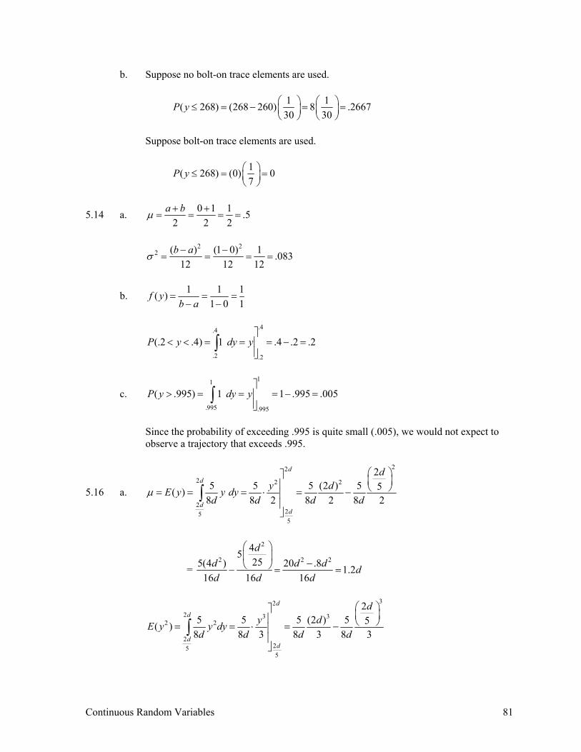
2 2 2 2 2 2( ) 1.6533 (1.2 ) .2133E y d d dσ μ= − = − − 2.2133 .46d dσ = =
1.2 .46 (.74 , 1.66 )d d d dμ σ± ⇒ ± ⇒
2 1.2 2(.46) (.28 , 2.12 )d d d dμ σ± ⇒ ± ⇒
b. 2
255
255 5 5 3 35( )
8 8 8 8 8 8
d
d
dd
dd dP y d dy
d d d d d
⎛ ⎞⎤ ⎜ ⎟⎥ ⎝ ⎠< = = = − = =⎥⎥⎦
∫
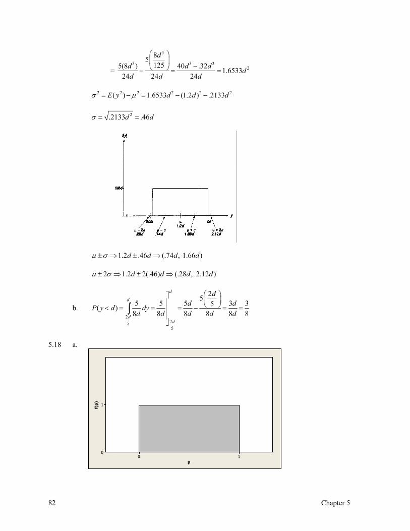
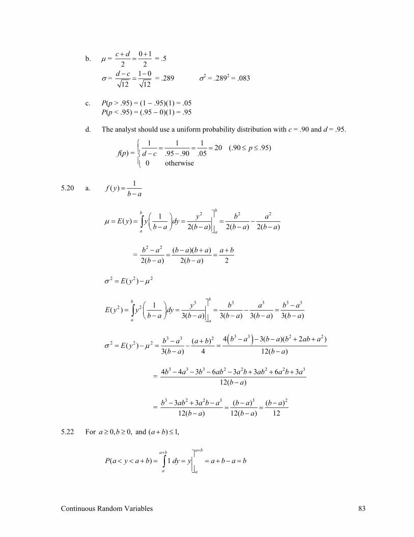
5.18 a.
p
f(p)
10
1
0
Continuous Random Variables 83
b. μ = 0 12 2
c d+ += = .5
σ = 1 012 12
d c− −= = .289 σ2 = .2892 = .083
c. P(p > .95) = (1 − .95)(1) = .05 P(p < .95) = (.95 − 0)(1) = .95 d. The analyst should use a uniform probability distribution with c = .90 and d = .95.
f(p) = 1 1 1 20 (.90 .95)
.95 .90 .050 otherwise
pd c
⎧ = = = ≤ ≤⎪− −⎨
⎪⎩
5.20 a. 1( )f yb a
=−
2 2 21( )
2( ) 2( ) 2( )
bb
a a
y b aE y y dyb a b a b a b a
μ⎤⎛ ⎞= = = = −⎥⎜ ⎟− − − −⎝ ⎠ ⎥⎦
∫
= 2 2 ( )( )
2( ) 2( ) 2b a b a b a a b
b a b a− − + +
= =− −
2 2 2( )E yσ μ= −
3 3 3 3 3
2 2 1( )3( ) 3( ) 3( ) 3( )
bb
a a
y b a b aE y y dyb a b a b a b a b a
⎤ −⎛ ⎞= = = − =⎥⎜ ⎟− − − − −⎝ ⎠ ⎥⎦∫
( )3 3 2 23 3 2
2 2 24 3( )( 2 )( )( )
3( ) 4 12( )
b a b a b ab ab a a bE yb a b a
σ μ− − − + +− +
= − = − =− −
= 3 3 3 2 2 2 2 34 4 3 6 3 3 6 3
12( )b a b ab a b ab a b a
b a− − − − + + +
−
= 3 2 2 3 3 23 3 ( ) ( )
12( ) 12( ) 12b ab a b a b a b a
b a b a− + − − −
= =− −
5.22 For 0, 0, and ( ) 1,a b a b≥ ≥ + ≤
( ) 1a ba b
a a
P a y a b dy y a b a b++ ⎤
< < + = = = + − =⎥⎥⎦
∫
84 Chapter 5
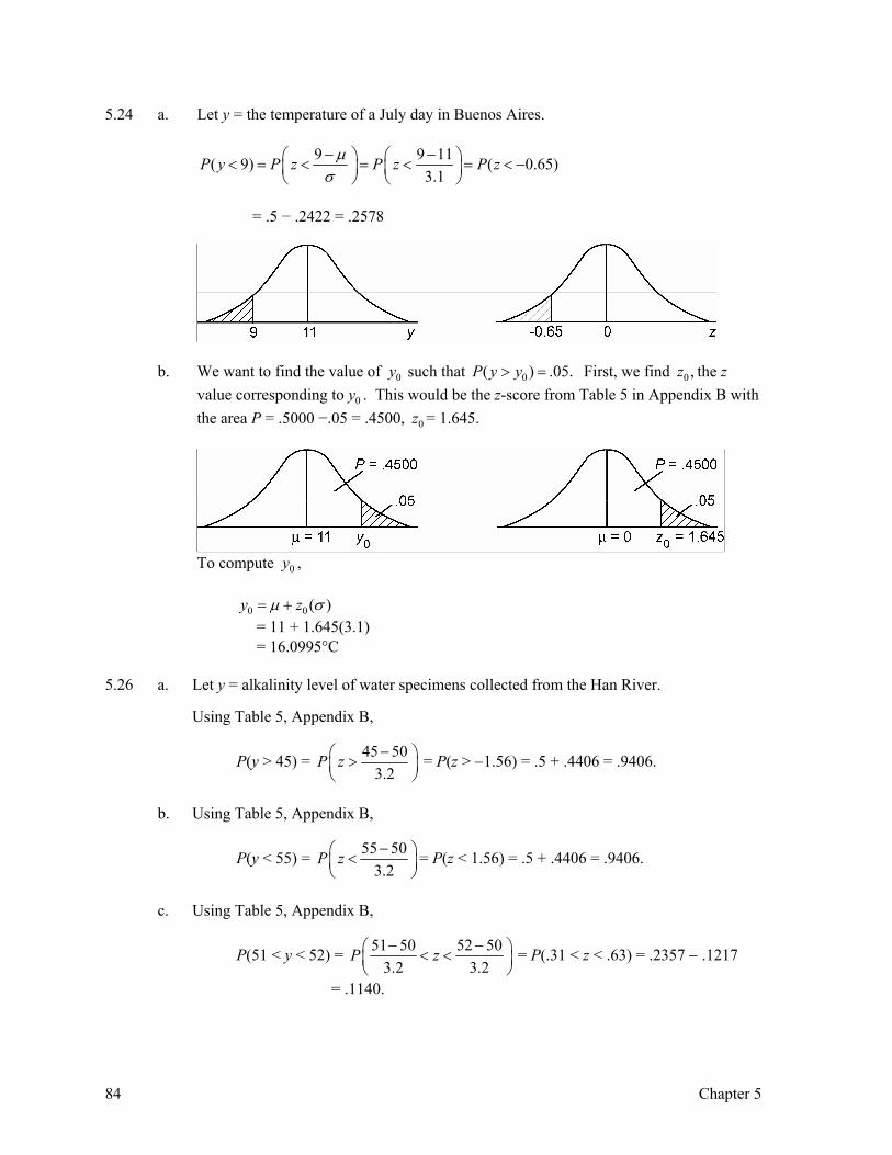
5.24 a. Let y = the temperature of a July day in Buenos Aires.
9 9 11( 9) ( 0.65)3.1
P y P z P z P zμσ− −⎛ ⎞ ⎛ ⎞< = < = < = < −⎜ ⎟ ⎜ ⎟
⎝ ⎠ ⎝ ⎠
= .5 − .2422 = .2578
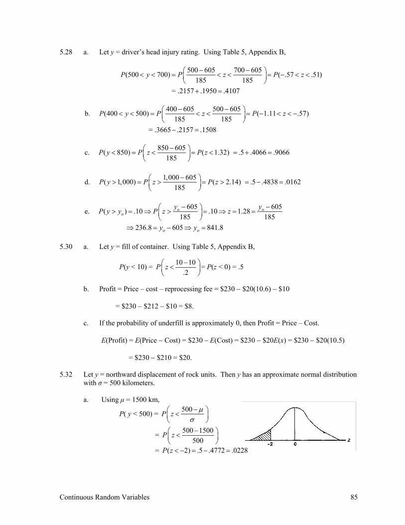
b. We want to find the value of 0y such that 0( ) .05.P y y> = First, we find 0 ,z the z
value corresponding to 0y . This would be the z-score from Table 5 in Appendix B with the area P = .5000 −.05 = .4500, 0z = 1.645.
To compute 0y , 0 0 ( )y zμ σ= + = 11 + 1.645(3.1) = 16.0995°C 5.26 a. Let y = alkalinity level of water specimens collected from the Han River. Using Table 5, Appendix B,
P(y > 45) = 45 503.2
P z −⎛ ⎞>⎜ ⎟⎝ ⎠
= P(z > −1.56) = .5 + .4406 = .9406.
b. Using Table 5, Appendix B,
P(y < 55) = 55 503.2
P z −⎛ ⎞<⎜ ⎟⎝ ⎠
= P(z < 1.56) = .5 + .4406 = .9406.
c. Using Table 5, Appendix B,
P(51 < y < 52) = 51 50 52 503.2 3.2
P z− −⎛ ⎞< <⎜ ⎟⎝ ⎠
= P(.31 < z < .63) = .2357 − .1217
= .1140.
Continuous Random Variables 85
5.28 a. Let y = driver’s head injury rating. Using Table 5, Appendix B,
500 605 700 605(500 700) ( .57 .51)
185 185 = .2157 .1950 .4107
P y P z P z− −⎛ ⎞< < = < < = − < <⎜ ⎟⎝ ⎠
+ =
400 605 500 605b. (400 500) ( 1.11 .57)
185 185 = .3665 .2157 .1508
P y P z P z− −⎛ ⎞< < = < < = − < < −⎜ ⎟⎝ ⎠
− =
850 605c. ( 850) ( 1.32) .5 .4066 .9066185
P y P z P z−⎛ ⎞< = < = < = + =⎜ ⎟⎝ ⎠
1,000 605d. ( 1,000) ( 2.14) .5 .4838 .0162185
P y P z P z−⎛ ⎞> = > = > = − =⎜ ⎟⎝ ⎠
605 605e. ( ) .10 .10 1.28
185 185 236.8 605 841.8
o oo
o o
y yP y y P z z
y y
− −⎛ ⎞> = ⇒ > = ⇒ = =⎜ ⎟⎝ ⎠
⇒ = − ⇒ =
5.30 a. Let y = fill of container. Using Table 5, Appendix B,
P(y < 10) = 10 10.2
P z −⎛ ⎞<⎜ ⎟⎝ ⎠
= P(z < 0) = .5
b. Profit = Price – cost – reprocessing fee = $230 − $20(10.6) − $10 = $230 − $212 − $10 = $8. c. If the probability of underfill is approximately 0, then Profit = Price – Cost. E(Profit) = E(Price − Cost) = $230 – E(Cost) = $230 − $20E(x) = $230 − $20(10.5)
= $230 − $210 = $20.
5.32 Let y = northward displacement of rock units. Then y has an approximate normal distribution
with σ = 500 kilometers. a. Using μ = 1500 km,
P( y < 500) = 500P z μσ−⎛ ⎞<⎜ ⎟
⎝ ⎠
= 500 1500500
P z −⎛ ⎞<⎜ ⎟⎝ ⎠
= ( 2) .5 .4772 .0228P z < − = − =
86 Chapter 5
b. Using μ = 1200 km,
500( 500)P y P z μσ−⎛ ⎞< = <⎜ ⎟
⎝ ⎠
= 500 1200500
P z −⎛ ⎞<⎜ ⎟⎝ ⎠
= P(z < −1.4) = .5 − .4192 = .0808 c. It is more likely the mean of 1200 is more plausible as this value led to a higher
probability for a displacement less than 500 km. 5.34 To determine if the data are approximately normal, we need to check to determine if the value
of IQR s ≈ 1.3.
U LIQR 6 1 5IQR 5/ 6.09 0.821
Q Qs= − = − =
= =
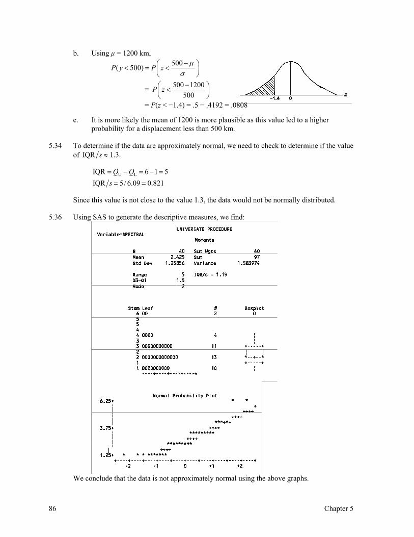
Since this value is not close to the value 1.3, the data would not be normally distributed. 5.36 Using SAS to generate the descriptive measures, we find:
We conclude that the data is not approximately normal using the above graphs.
Continuous Random Variables 87
5.38 From the graph, the data appear to be very mound-shaped. It appears that the data are approximately normally distributed.
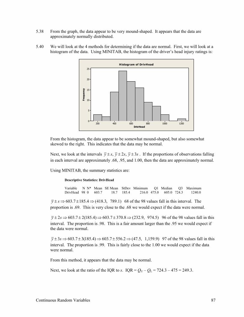
5.40 We will look at the 4 methods for determining if the data are normal. First, we will look at a histogram of the data. Using MINITAB, the histogram of the driver’s head injury ratings is:
DrivHead
Freq
uenc
y
12001000800600400200
25
20
15
10
5
0
Histogram of DrivHead
From the histogram, the data appear to be somewhat mound-shaped, but also somewhat skewed to the right. This indicates that the data may be normal. Next, we look at the intervals , 2 , 3y s y s y s± ± ± . If the proportions of observations falling in each interval are approximately .68, .95, and 1.00, then the data are approximately normal. Using MINITAB, the summary statistics are:
Descriptive Statistics: DrivHead Variable N N* Mean SE Mean StDev Minimum Q1 Median Q3 Maximum DrivHead 98 0 603.7 18.7 185.4 216.0 475.0 605.0 724.3 1240.0
603.7 185.4 (418.3, 789.1)y s± ⇒ ± ⇒ 68 of the 98 values fall in this interval. The
proportion is .69. This is very close to the .68 we would expect if the data were normal.
2 603.7 2(185.4) 603.7 370.8 (232.9, 974.5)y s± ⇒ ± ⇒ ± ⇒ 96 of the 98 values fall in this interval. The proportion is .98. This is a fair amount larger than the .95 we would expect if the data were normal.
3 603.7 3(185.4) 603.7 556.2 (47.5, 1,159.9)y s± ⇒ ± ⇒ ± ⇒ 97 of the 98 values fall in this interval. The proportion is .99. This is fairly close to the 1.00 we would expect if the data were normal. From this method, it appears that the data may be normal. Next, we look at the ratio of the IQR to s. IQR = QU – QL = 724.3 – 475 = 249.3.
88 Chapter 5
IQR 249.3 1.3185.4s
= = This is equal to the 1.3 we would expect if the data were normal. This
method indicates the data may be normal.
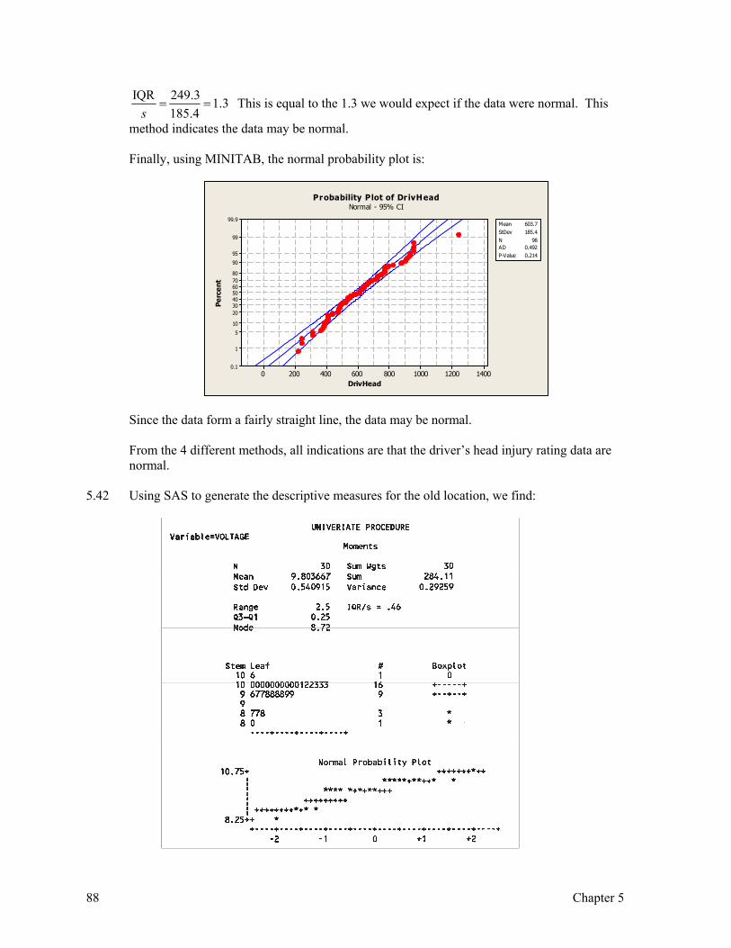
Finally, using MINITAB, the normal probability plot is:
DrivHead
Perc
ent
1400120010008006004002000
99.9
99
95
90
80706050403020
10
5
1
0.1
Mean
0.214
603.7StDev 185.4N 98AD 0.492P-Value
Probability Plot of Dr ivHeadNormal - 95% CI
Since the data form a fairly straight line, the data may be normal. From the 4 different methods, all indications are that the driver’s head injury rating data are normal.
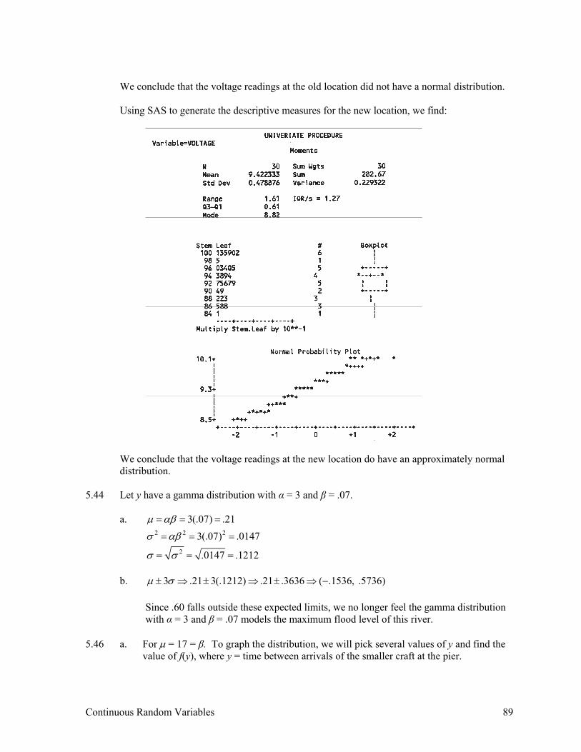
5.42 Using SAS to generate the descriptive measures for the old location, we find:
Continuous Random Variables 89
We conclude that the voltage readings at the old location did not have a normal distribution. Using SAS to generate the descriptive measures for the new location, we find:
We conclude that the voltage readings at the new location do have an approximately normal distribution.
5.44 Let y have a gamma distribution with α = 3 and β = .07. a. 3(.07) .21μ αβ= = = 2 2 23(.07) .0147σ αβ= = =
2 .0147 .1212σ σ= = = b. 3 .21 3(.1212) .21 .3636 ( .1536, .5736)μ σ± ⇒ ± ⇒ ± ⇒ − Since .60 falls outside these expected limits, we no longer feel the gamma distribution
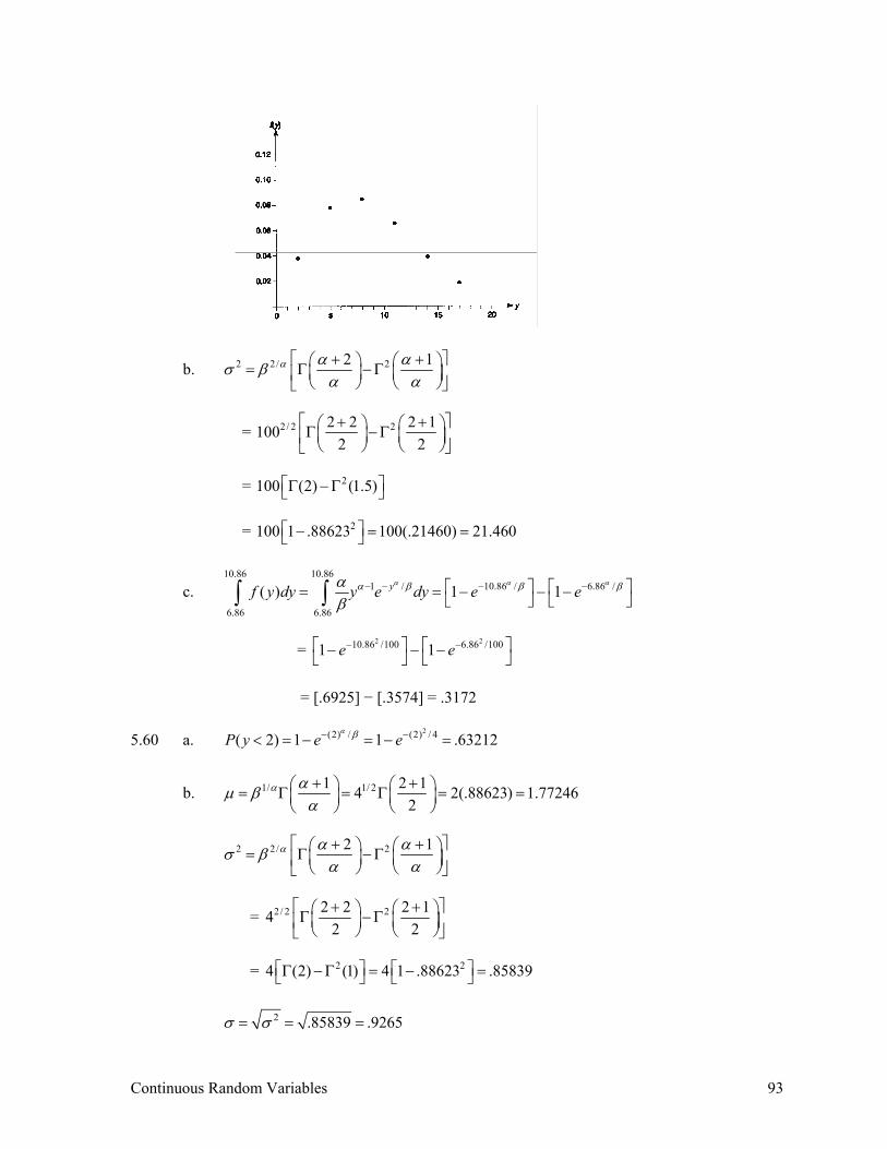
with α = 3 and β = .07 models the maximum flood level of this river. 5.46 a. For μ = 17 = β. To graph the distribution, we will pick several values of y and find the
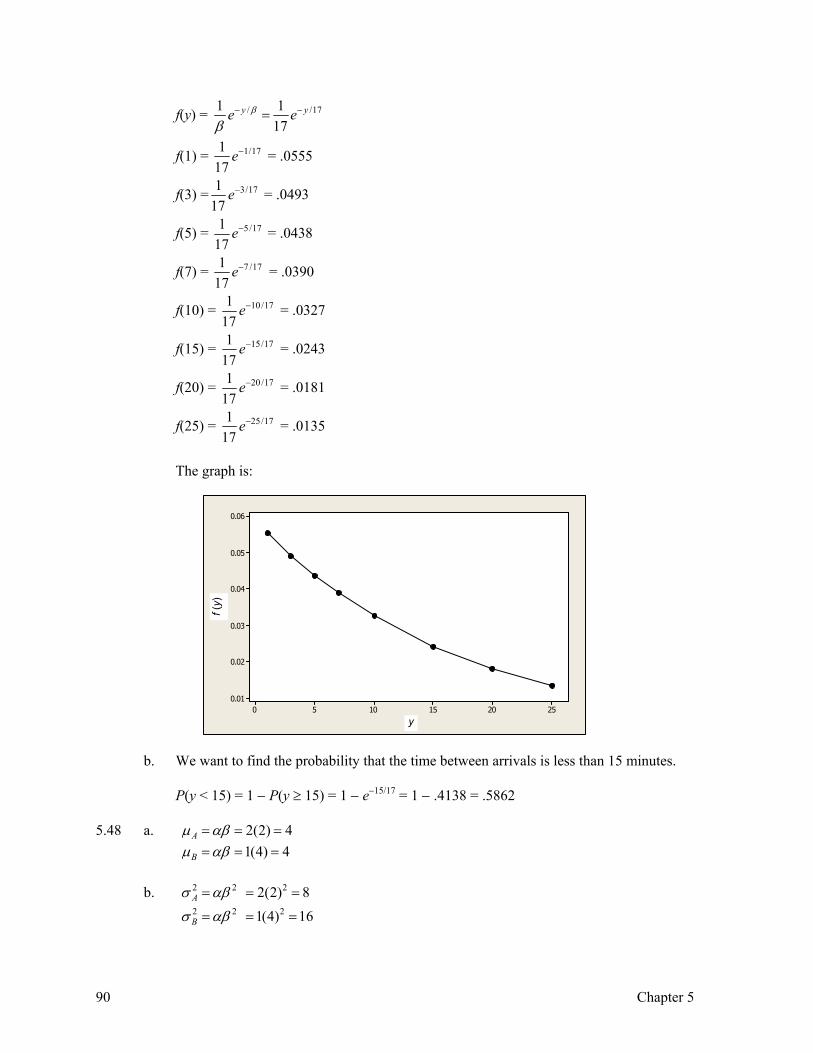
value of f(y), where y = time between arrivals of the smaller craft at the pier.
90 Chapter 5
f(y) = / /171 117
y ye eβ
β− −=
f(1) = 1/17117
e− = .0555
f(3) = 3/17117
e− = .0493
f(5) = 5/17117
e− = .0438
f(7) = 7 /17117
e− = .0390
f(10) = 10/17117
e− = .0327
f(15) = 15/17117
e− = .0243
f(20) = 20/17117
e− = .0181
f(25) = 25/17117
e− = .0135
The graph is:
x
f(x)
2520151050
0.06
0.05
0.04
0.03
0.02
0.01
b. We want to find the probability that the time between arrivals is less than 15 minutes. P(y < 15) = 1 − P(y ≥ 15) = 1 − e−15/17 = 1 − .4138 = .5862 5.48 a. 2(2) 4Aμ αβ= = = 1(4) 4Bμ αβ= = = b. 2 2 22(2) 8Aσ αβ= = = 2 2 21(4) 16Bσ αβ= = =
y
f (y)
Continuous Random Variables 91
c. For A: 1 1/ 2 / 2
0 0
( 1)4 (2) 4
y yye yeP y dy dy− −
< = =Γ∫ ∫
= 1 1
1/ 2 / 2 / 20
0 0
1 1 2 24 4
y y yye dy ye e dy− − −⎡ ⎤
⎤= − +⎢ ⎥⎦⎢ ⎥⎣ ⎦∫ ∫
= 1/ 20
1 ( 1.213 0) 44
ye−⎡ ⎤⎤− − + − ⎦⎢ ⎥⎣ ⎦
= [ ]1 1.213 ( 2.426) 4 .09024− + − + =
For B: 1 1/ 4
/ 4
0 0
1( 1)4 (1) 4
yyeP y dy e dy
−−< = =
Γ∫ ∫
= [ ]1/ 40
4 3.115 ( 4) .8847ye− ⎤− = − − − =⎦
B has the higher probability. 5.50 a. 25,000( ) ( ) t tR t P Y t e eμ− −= ≥ = = b. 8,760 25,000 .3504( 8,760) 0.7044P Y e e− −≥ = = = c. S(t) = P(at least one drive has a lifelength that exceeding t hours) = 1 − P(neither
exceeds t hours)
[ ]22 25,000( ) 1 1 ( ) 1 1 tS t R t e−⎡ ⎤= − − = − −⎣ ⎦
d. [ ]2 2 28,760 25,000 .3504(8,760) 1 1 1 1 1 .2956 1 0.0874 0.9126S e e− −⎡ ⎤ ⎡ ⎤= − − = − − = − = − =⎣ ⎦ ⎣ ⎦
5.52 1 / ( 2) 1 /
2 2 2
0 0
( ) ( )( ) ( )
y yy e y eE y y f y dy y dy dyα β α β
α αβ α β α
∞ ∞ ∞− − + − −
−∞
= = =Γ Γ∫ ∫ ∫
Multiplying and dividing by 2 ( 1)αβ α + , we get
= ( 2) 1 /
2( 2)
0
( 1)( 1) ( )
yy e dyα β
ααβ αβ α α α
∞ + − −
+++ Γ∫
= ( 2) 1 /
2 2( 2)
0
( 1) ( 1)( 2)
yy e dyα β
ααβ α αβ αβ α
∞ + − −
++ = +Γ +∫
2 2 2 2 2 2 2 2 2 2 2( ) ( 1) ( )E yσ μ αβ α αβ α β αβ α β αβ= − = + − = + − =
92 Chapter 5
5.54 /( ) 1 0yF y e yβ−= − ≤ ≤ ∞ ( ) /( ) 1 ( ) x yF x y F x y e β− ++ = − + = /( ) 1 ( ) xF x F x e β−= − = /( ) 1 ( ) yF y F y e β−= − = / / ( ) /( ) ( ) x y x yF x F y e e eβ β β− − − += = ( ) ( ) ( )F x y F x F y⇒ + = ⇒ Both NBU and NWU 5.56 / 2 2v vμ αβ= = ⋅ =
2 2 2/ 2 (2) 2v vσ αβ= = ⋅ =
5.58 a. 1 /( ) , 0yf y y e yαα βα
β− −= ≥
For α = 2, β = 100, 2 /1002( ) 0
100yf y y e y−= ≥
22 /100 .042 2(2) .03843
50 50f e e− −= = =
25 /100 .255 5(5) .07788
50 50f e e− −= = =
28 /100 .648 8(8) .08437
50 50f e e− −= = =
211 /100 1.2111 11(11) .06560
50 50f e e− −= = =
214 /100 1.9614 14(14) .03944
50 50f e e− −= = =
217 /100 2.8917 17(17) .018896
50 50f e e− −= = =
Continuous Random Variables 93
b. 2 2/ 22 1α α ασ βα α
⎡ ⎤+ +⎛ ⎞ ⎛ ⎞= Γ −Γ⎜ ⎟ ⎜ ⎟⎢ ⎥⎝ ⎠ ⎝ ⎠⎣ ⎦
= 2/ 2 22 2 2 11002 2
⎡ ⎤+ +⎛ ⎞ ⎛ ⎞Γ −Γ⎜ ⎟ ⎜ ⎟⎢ ⎥⎝ ⎠ ⎝ ⎠⎣ ⎦
= 2100 (2) (1.5)⎡ ⎤Γ −Γ⎣ ⎦
= 2100 1 .88623 100(.21460) 21.460⎡ ⎤− = =⎣ ⎦
c. 10.86 10.86
1 / 10.86 / 6.86 /
6.86 6.86
( ) 1 1yf y dy y e dy e eα α αα β β βα
β− − − −⎡ ⎤ ⎡ ⎤= = − − −⎣ ⎦ ⎣ ⎦∫ ∫
= 2 210.86 /100 6.86 /1001 1e e− −⎡ ⎤ ⎡ ⎤− − −⎣ ⎦ ⎣ ⎦
= [.6925] − [.3574] = .3172 5.60 a.
2(2) / (2) / 4( 2) 1 1 .63212P y e eα β− −< = − = − =
b. 1/ 1/ 21 2 14 2(.88623) 1.772462
α αμ βα+ +⎛ ⎞ ⎛ ⎞= Γ = Γ = =⎜ ⎟ ⎜ ⎟
⎝ ⎠ ⎝ ⎠
2 2/ 22 1α α ασ βα α
⎡ ⎤+ +⎛ ⎞ ⎛ ⎞= Γ −Γ⎜ ⎟ ⎜ ⎟⎢ ⎥⎝ ⎠ ⎝ ⎠⎣ ⎦
= 2/ 2 22 2 2 142 2
⎡ ⎤+ +⎛ ⎞ ⎛ ⎞Γ −Γ⎜ ⎟ ⎜ ⎟⎢ ⎥⎝ ⎠ ⎝ ⎠⎣ ⎦
= 2 24 (2) (1) 4 1 .88623 .85839⎡ ⎤ ⎡ ⎤Γ −Γ = − =⎣ ⎦ ⎣ ⎦
2 .85839 .9265σ σ= = =
94 Chapter 5
c. [ ]( 2 2 ) 1.77 2(.9265) 1.77 2(.9265)P y P yμ σ μ σ− ≤ ≤ + = − ≤ ≤ + = ( .083 3.623)P y− ≤ ≤
= 2
3.623(3.623) / (3.623) / 4
0
( ) 1 1f y dy e eα β− −= − = −∫
= 1 − .0376 = .9624 d.
2(6) / 4( 6) 1 ( 6) 1 1P y P y e−⎡ ⎤> = − < = − −⎣ ⎦
= 1 − [1 −.0001234] = 1 − .999876 = .0001234 This is very unlikely. 5.62 We want to find the value of 0y such that 0( )P y y< = .05
20 0( ) / ( ) / 60
0( ) 1 1y yP y y e eα β− −< = − = −
20( ) / 60 .95ye−⇒ =
2
0( ) / 60 ln(.95)y⇒− = 2
0( ) 60 ln(.95)y⇒− = 2
0 60 ln(.95)y⇒ = − 0 60 ln(.95)y⇒ = − 0 3.0776y⇒ = 0y⇒ = 1.7543 5.64 If y has a Weibull distribution, then
1 / 0
( )0 elsewhere
yy e yf y
αα βαβ
− −⎧ ≤ < ∞⎪= ⎨⎪⎩
2 1 / 1 2 /
0 0
1( ) y yE y y e dy y y e dyα αα β α βα α
β β
∞ ∞+ − − −= =∫ ∫
Continuous Random Variables 95
Let .z yα= Then 1 .dz y dyα−= 0 0 0y z α= ⇒ = = y z α= ∞⇒ = ∞ = ∞
Thus, 2 2 / /
0
1( ) zE y z e dzα β
β
∞−= ∫
We know from the Gamma distribution that 1 /
0
( )yy eα β αα β∞
− − = Γ∫
So, 2 2/ / (2 / ) 1 2/
0
1 1 2 2( ) 1zE y z e dzα β α ααβ ββ β α α
∞− + +⎛ ⎞ ⎛ ⎞= = Γ + = Γ⎜ ⎟ ⎜ ⎟
⎝ ⎠ ⎝ ⎠∫
From Exercise 5.63, 1/ 1α αμ βα+⎛ ⎞= Γ⎜ ⎟
⎝ ⎠
Thus, 2 2 2 2/ 2 / 22 1( )E y α αα ασ μ β βα α+ +⎛ ⎞ ⎛ ⎞= − = Γ − Γ⎜ ⎟ ⎜ ⎟
⎝ ⎠ ⎝ ⎠
= 2/ 22 1α α αβα α
⎡ ⎤+ +⎛ ⎞ ⎛ ⎞Γ −Γ⎜ ⎟ ⎜ ⎟⎢ ⎥⎝ ⎠ ⎝ ⎠⎣ ⎦
5.66 a. The probability density function when 2 and 2n n Nα β= = is:
2 1 2 1(1 )( )( 2, 2 )
n n Ny yf yB n n N
− −−=
b. For this problem, we let n = 10 and N=100.
2 10 / 2 0.9900992 2 10 / 2 10 /(2)(100)
nn n N
αμα β
= = = =+ + +
22 2
( / 2)( / 2 )( ) ( 1) ( 2 2 ) ( 2 2 1)
n n Nn n N n n N
αβσα β α β
= =+ + + + + +
2(10 / 2)[10 / 2(100)] 0.0016203
[10 / 2 10 / 2(100)] [10 / 2 (10 / 2(100) 1]= =
+ + +
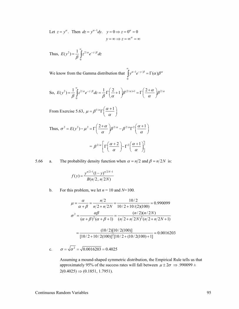
c. 2 0.0016203 0.4025σ σ= = = Assuming a mound-shaped symmetric distribution, the Empirical Rule tells us that
approximately 95% of the success rates will fall between 2μ σ± ⇒ .990099 ± 2(0.4025) ⇒ (0.1851, 1.7951).
96 Chapter 5
where 1 10 and .40n pα β= + − = = for a binomial distribution.
where p(y) is a binomial probability using n = α + β – 1 and p =.10.
where ( )p y is a binomial probability with 1 3n α β= + − = and p = .10.
5.68 a. 2 .181822 9
αμα β
= = =+ +
22 2
2(9) .0124( ) ( 1) (2 9) (2 9 1)
αβσα β α β
= = =+ + + − + +
b. ( )( .40) 1 ( .40) 1 .40P y P y F> = − < = −
= 1 ( ) n
y
p yα=
−∑
= 10 1
2 0
1 ( ) 1 1 ( ) from Table 2 of Appendix B.y y
p y p y= =
⎡ ⎤− = − −⎢ ⎥
⎢ ⎥⎣ ⎦∑ ∑
= .0464
c. ( .10) ( ) n
y
P y p yα=
< =∑
10 1
2 0
( ) =1 ( ) 1 .7361 .2639y y
p y p y= =
= − = − =∑ ∑
5.70 a. 2 .52 2
αμα β
= = =+ +
22 2 2
2(2) 4 .05( ) ( 1) (2 2) (2 2 1) 4 (5)
αβσα β α β
= = = =+ + + + + +
b. ( .10) (.10) ( )n
y
P y F p yα=
< = =∑
( .10)P y <3
2 1 3 0
2
3 3( ) = (.1) (.9) (.1) (.9) .027 .001 .028
2 3y
P y=
⎛ ⎞ ⎛ ⎞= + = + =⎜ ⎟ ⎜ ⎟
⎝ ⎠ ⎝ ⎠∑
5.72 1 1
0
(1 )( )( , )
y yE y dyB
α β
μα β
−−= = ∫
= 1 1
0
( 1, ) (1 )( , ) ( 1, )
B y y dyB B
α βα βα β α β
−+ −⋅
+∫
Continuous Random Variables 97
= 1 1
0
( 1) ( ) ( ) (1 )( 1) ( ) ( ) ( 1, )
y y dyα βα β α β
α β α β β α β
−Γ + Γ Γ + −⋅ ⋅
Γ + + Γ Γ +∫
= 1 1
0
( 1) ( ) ( ) (1 )( 1) ( ) ( ) ( 1, )
y y dyα βα α α β
α β α β α β α β
−+ Γ Γ + −⋅ ⋅
+ + Γ + Γ +∫
Let 1 1 1
0
(1 )1( , )
y y dyγ βγ γγ α
γ β β γ β γ β
− −−= + ⇒ ⋅ =
+ +∫
5.74 ( ) 1 ( ) 1 ( )n
y
F y F y p yα=
= − = −∑
= 2
2
2
1 ( ) 1 ( )y
p y y=
− = −∑
2( ) 1F x x= −
2( ) 1 ( )F x y x y+ = − +
2 2 2 2 2 2( ) ( ) (1 )(1 ) 1F x F y x y x y x y= − − = − − +
2 2 2 2( ) 1 ( 2 ) 1 2F x y x y xy x y xy+ = − + + = − − −
( ) ( ) ( ) for all , 0F x y F x F y x y⇒ + ≤ ≥ ⇒ NBU 5.76 ( ) (1 )m t t αβ −= − / 2α ν= β = 2
/ 2( ) (1 2 )m t t ν−⇒ = −
5.78 a. 0 0
( 1)( ) ( )ty ty y t ym t E e e e dy e dy+
−∞ −∞
= = =∫ ∫
= 0
( 1) 11 1( 1) ( 1)1 1
t yt e dy tt t
+ −
−∞
+ = = ++ +∫
b. 21
0 0
( ) 1( 1) 1t t
dm t tdt
μ μ −
= =
⎤⎤′ = = = − + = −⎥⎥⎦ ⎦
2
32 2
0 0
( ) 2( 1) 2t t
d m t tdt
μ −
= =
⎤⎤′ = = + =⎥⎥
⎥⎦ ⎦
( )22 2
2 1 2 ( 1) 2 1 1σ μ μ′ ′= − = − − = − =
where ( )p y is a binomial probability with 1 2 and n p yα β= + − = = .
98 Chapter 5
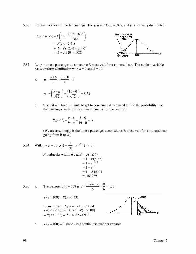
5.80 Let y = thickness of mortar coatings. For y, μ = .635, σ = .082, and y is normally distributed.
.4735 .635( .4375).082
P y P z −⎛ ⎞< = <⎜ ⎟⎝ ⎠
= ( 2.41)P z < − = .5 − P(−2.41 < z < 0) = .5 − .4920 = .0080
5.82 Let y = time a passenger at concourse B must wait for a monorail car. The random variable
has a uniform distribution with a = 0 and b = 10.
a. 0 10 52 2
a bμ + += = =
2 2
2 10 0 8.3312 12
b aσ − −⎛ ⎞ ⎛ ⎞= = =⎜ ⎟ ⎜ ⎟⎝ ⎠ ⎝ ⎠
b. Since it will take 1 minute to get to concourse A, we need to find the probability that
the passenger waits for less than 3 minutes for the next car.
3 0( 3) .310 0
c aP yb a− −
< = = =− −
(We are assuming y is the time a passenger at concourse B must wait for a monorail car
going from B to A.)
5.84 With μ = β = 30, f(y) = 130
⋅ e−y/30 (y > 0) P(outbreaks within 6 years) = P(y ≤ 6) = 1 − P(y > 6) = 1 − e−6/30 = 1 − e−.2 = 1 − .818731 = .181269
5.86 a. The z-score for y = 108 is 108 100 8 1.336 6
z −= = =
( 108) ( 1.33)P y P z> = > From Table 5, Appendix B, we find (0 1.33) .4082.P z< < = ( 108)P y > ( 1.33) .5 .4082 0918.P z= > = − =
b. ( 100) 0P y = = since y is a continuous random variable.
Continuous Random Variables 99
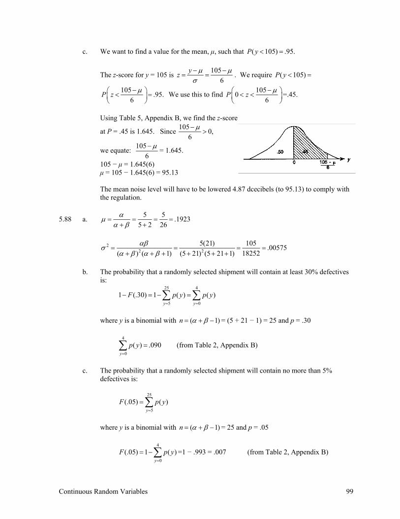
c. We want to find a value for the mean, μ, such that ( 105) .95.P y < =
The z-score for y = 105 is 1056
yz μ μσ− −
= = . We require ( 105)P y < =
105 .95.6
P z μ−⎛ ⎞< =⎜ ⎟⎝ ⎠
We use this to find 10506
P z μ−⎛ ⎞< <⎜ ⎟⎝ ⎠
=.45.
Using Table 5, Appendix B, we find the z-score
at P = .45 is 1.645. Since 105 0,6μ−>
we equate: 1056μ− = 1.645.
105 − μ = 1.645(6) μ = 105 − 1.645(6) = 95.13 The mean noise level will have to be lowered 4.87 dcecibels (to 95.13) to comply with
the regulation.
5.88 a. 5 5 .19235 2 26
αμα β
= = = =+ +
22 2
5(21) 105 .0057518252( ) ( 1) (5 21) (5 21 1)
αβσα β α β
= = = =+ + + + + +
b. The probability that a randomly selected shipment will contain at least 30% defectives
is:
25 4
5 0
1 (.30) 1 ( ) ( )y y
F p y p y= =
− = − =∑ ∑
where y is a binomial with ( 1)n α β= + − = (5 + 21 − 1) = 25 and p = .30
4
0
( ) .090y
p y=
=∑ (from Table 2, Appendix B)
c. The probability that a randomly selected shipment will contain no more than 5%
defectives is:
25
5
(.05) ( )y
F p y=
=∑
where y is a binomial with ( 1)n α β= + − = 25 and p = .05
4
0
(.05) 1 ( )y
F p y=
= −∑ =1 − .993 = .007 (from Table 2, Appendix B)
100 Chapter 5
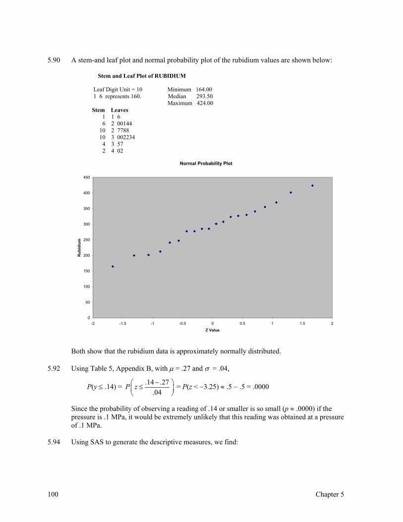
5.90 A stem-and leaf plot and normal probability plot of the rubidium values are shown below:
Stem and Leaf Plot of RUBIDIUM Leaf Digit Unit = 10 Minimum 164.00 1 6 represents 160. Median 293.50 Maximum 424.00
Stem Leaves 1 1 6 6 2 00144 10 2 7788 10 3 002234 4 3 57 2 4 02
Normal Probability Plot
0
50
100
150
200
250
300
350
400
450
-2 -1.5 -1 -0.5 0 0.5 1 1.5 2
Z Value
Rub
idiu
m
Both show that the rubidium data is approximately normally distributed.
5.92 Using Table 5, Appendix B, with μ = .27 and σ = .04,
P(y ≤ .14) = .14 .27.04
P z −⎛ ⎞≤⎜ ⎟⎝ ⎠
= P(z < −3.25) ≈ .5 − .5 = .0000
Since the probability of observing a reading of .14 or smaller is so small (p ≈ .0000) if the
pressure is .1 MPa, it would be extremely unlikely that this reading was obtained at a pressure of .1 MPa.
5.94 Using SAS to generate the descriptive measures, we find:
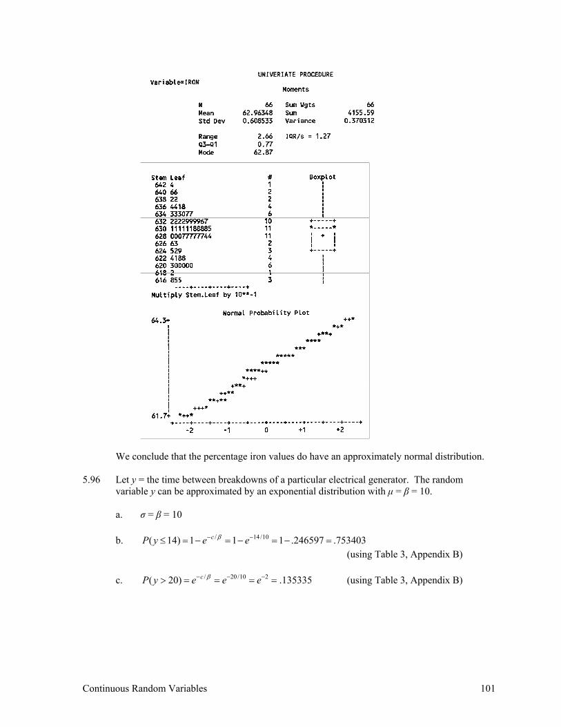
Continuous Random Variables 101
We conclude that the percentage iron values do have an approximately normal distribution. 5.96 Let y = the time between breakdowns of a particular electrical generator. The random
variable y can be approximated by an exponential distribution with μ = β = 10. a. σ = β = 10 b. / 14/10( 14) 1 1 1 .246597 .753403cP y e eβ− −≤ = − = − = − = (using Table 3, Appendix B) c. / 20 /10 2( 20) .135335cP y e e eβ− − −> = = = = (using Table 3, Appendix B)
102 Chapter 5
5.98 a. α = 2, β = 16
b. 1/ 1/ 21 316 4(.88623) 3.5452
α αμ βα+⎡ ⎤ ⎛ ⎞= Γ = Γ = =⎜ ⎟⎢ ⎥⎣ ⎦ ⎝ ⎠
(from Table 6, Appendix B)
2 2/ 2 2 / 2 22 1 316 (2)2
α α ασ βα α
⎡ ⎤ ⎡ ⎤+ +⎛ ⎞ ⎛ ⎞ ⎛ ⎞= Γ −Γ = Γ −Γ⎜ ⎟ ⎜ ⎟ ⎜ ⎟⎢ ⎥ ⎢ ⎥⎝ ⎠ ⎝ ⎠ ⎝ ⎠⎣ ⎦ ⎣ ⎦
= [ ]216 1 (.88623) 16 .2145964 3.434⎡ ⎤− = =⎣ ⎦
c. ( 6) 1 ( 6) 1 (6)P y P y F≥ = − < = −
= /(6)1 1 e
α β−⎡ ⎤− −⎣ ⎦
= 2(6) /16 2.25 .1054e e− −= =
5.100 a. We know ( ) 1f y dy∞
−∞
=∫
Thus, 2
0
1ycye∞
− =∫
2 2 2( ) 0
01 0 1 2
2 2 2 2yc c c ce e e c
∞− − ∞ −− − −⎤ ⎛ ⎞⇒ = ⇒ − = + = ⇒ =⎜ ⎟⎥⎦ ⎝ ⎠
b. 2
0 0
( ) ( ) ( ) 2y y
tf y P Y y f t dt te dt−= < = =∫ ∫
Let 2 1/ 2 20 0z t z t t y z y= ⇒ = ≤ ≤ ⇒ ≤ ≤
Then 1/ 21 12 or 2 2
dz t dt dt dz z dzt
−= = =
( )2
2 2
2 21/ 2 1/ 2 0
0 0 0
1( ) 2 12
yy y
z z z y yF y z e z dz e dz e e e e− − − − − − −⎤⎛ ⎞ ⎥= = = − = − − − = −⎜ ⎟ ⎥⎝ ⎠ ⎦
∫ ∫
c.
22.5 6.25( 2.5) 1 ( 2.5) 1 (2.5) 1 1 .00193P y P y F e e− −⎡ ⎤> = − ≤ = − = − − = =⎣ ⎦
Continuous Random Variables 103
5.102 a. ( ) ( )( ) ( )y a t y a ty am t E e e f y dy+ ++ ⎡ ⎤= =⎣ ⎦ ∫
= ( ) ( )yt at at yte e f y dy e e f y dy=∫ ∫
= ( )atye m t
b. ( ) ( )( ) ( ) ( ) ( )by t byt y bt
by ym t E e e f y dy e f y dy m bt⎡ ⎤= = = =⎣ ⎦ ∫ ∫
c. [ ]
( ) / / /( ) / ( ) ( )y a t b at b yt by a bm t E e e e f y dy++
⎡ ⎤= =⎣ ⎦ ∫
= / ( / ) ( )at b y t be e f y dy∫
= / ( / )at b
ye m t b