Solution (a,b). 2 Solution (c). y t x y epunshs/Files/MATH246/SampFinalsol.pdf · Solutions to Final Exam Sample Problems, Math 246, Fall 2013 (1) Consider the diﬀerential equation

Solutions to Final Exam Sample Problems, Math 246, Fall 2013

(1) Consider the differential equationdy

dt= (9− y2)y2.

(a) Identify its stationary points and classify their stability.(b) Sketch its phase-line portrait in the interval −5 ≤ y ≤ 5.(c) If y(0) = −1, how does the solution y(t) behave as t→∞?

Solution (a,b). The right-hand side factors as (3 + y)(3 − y)y2. The stationarysolutions are y = −3, y = 0, and y = 3. Therefore a sign analysis of (3 + y)(3− y)y2

shows that the phase-line portrait for this equation is

− + + −←←←← • →→→→ • →→→→ • ←←←← y

−3 0 3unstable semistable stable

Solution (c). The phase-line shows that if y(0) = −1 then y(t)→ 0 as t→∞.

(2) Solve (possibly implicitly) each of the following initial-value problems. Identify theirintervals of definition.

(a)dy

dt+

2ty

1 + t2= t2 , y(0) = 1 .

(b)dy

dx+

exy + 2x

2y + ex= 0 , y(0) = 0 .

Solution (a). This equation is linear and is already in normal form. An integratingfactor is

exp

(∫ t

0

2s

1 + s2ds

)

= exp(

log(1 + t2))

= 1 + t2 ,

so that the integrating factor form is

d

dt

(

(1 + t2)y)

= (1 + t2)t2 = t2 + t4 .

Integrate this to obtain

(1 + t2)y = 13t3 + 1

5t5 + c .

The initial condition y(0) = 1 implies that c = (1+02) · 1− 1303− 1

505 = 1. Therefore

y =1 + 1

3t3 + 1

5t5

1 + t2.

This solution exists for every t, so its interval of definition is (−∞,∞).

Remark. Because this equation is linear, we can see that the interval of definitionof its solution is (−∞,∞) without solving it because both its coefficient and forcingare continuous over (−∞,∞).

Solution (b). The initial-value problem is

dy

dx+

exy + 2x

2y + ex= 0 , y(0) = 0 .

1

2

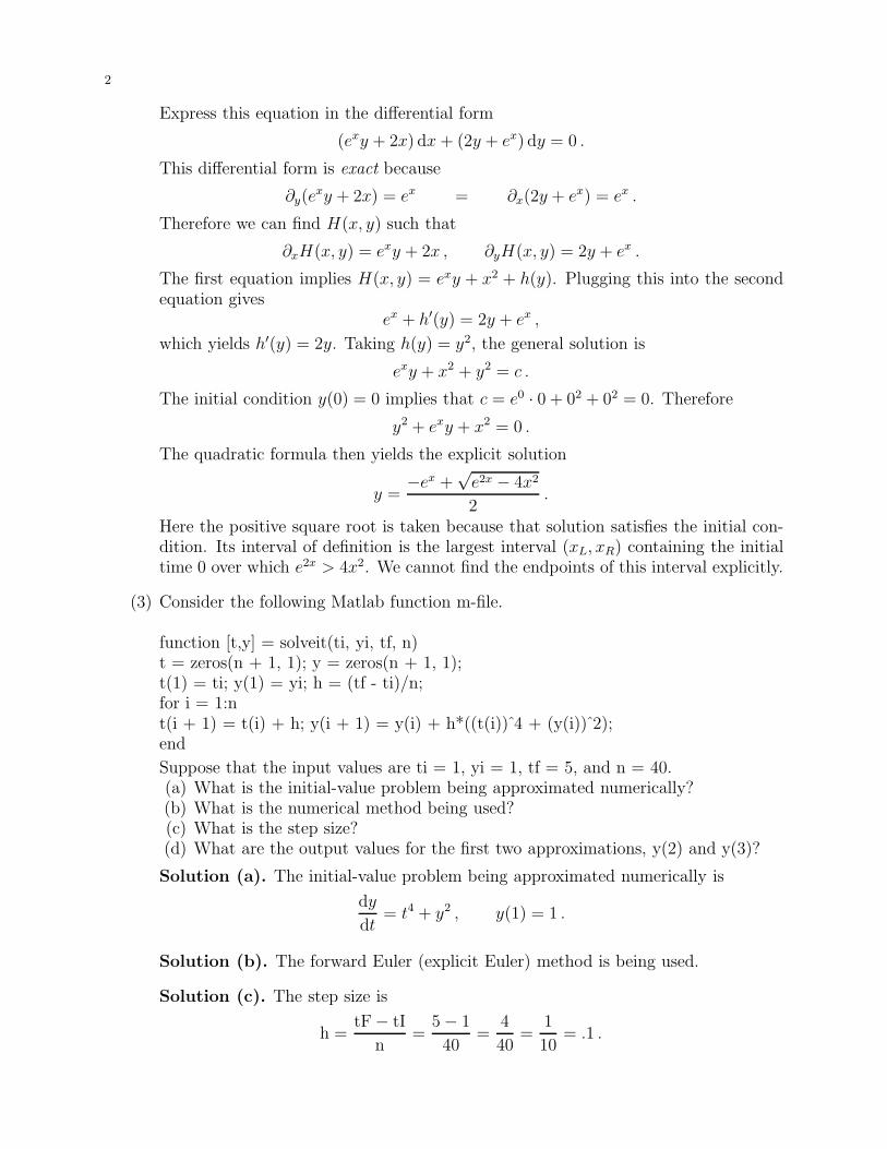
Express this equation in the differential form

(exy + 2x) dx+ (2y + ex) dy = 0 .

This differential form is exact because

∂y(exy + 2x) = ex = ∂x(2y + ex) = ex .

Therefore we can find H(x, y) such that

∂xH(x, y) = exy + 2x , ∂yH(x, y) = 2y + ex .

The first equation implies H(x, y) = exy + x2 + h(y). Plugging this into the secondequation gives

ex + h′(y) = 2y + ex ,

which yields h′(y) = 2y. Taking h(y) = y2, the general solution is

exy + x2 + y2 = c .

The initial condition y(0) = 0 implies that c = e0 · 0 + 02 + 02 = 0. Therefore

y2 + exy + x2 = 0 .

The quadratic formula then yields the explicit solution

y =−ex +

√e2x − 4x2

2.

Here the positive square root is taken because that solution satisfies the initial con-dition. Its interval of definition is the largest interval (xL, xR) containing the initialtime 0 over which e2x > 4x2. We cannot find the endpoints of this interval explicitly.

(3) Consider the following Matlab function m-file.

function [t,y] = solveit(ti, yi, tf, n)t = zeros(n + 1, 1); y = zeros(n + 1, 1);t(1) = ti; y(1) = yi; h = (tf - ti)/n;for i = 1:nt(i + 1) = t(i) + h; y(i + 1) = y(i) + h*((t(i))̂ 4 + (y(i))̂ 2);end

Suppose that the input values are ti = 1, yi = 1, tf = 5, and n = 40.(a) What is the initial-value problem being approximated numerically?(b) What is the numerical method being used?(c) What is the step size?(d) What are the output values for the first two approximations, y(2) and y(3)?

Solution (a). The initial-value problem being approximated numerically is

dy

dt= t4 + y2 , y(1) = 1 .

Solution (b). The forward Euler (explicit Euler) method is being used.

Solution (c). The step size is

h =tF− tI

n=

5− 1

40=

4

40=

1

10= .1 .

3

Solution (d). By carrying out the “for” loop in the Matlab code for i = 1 and i = 2we obtain the output values

t(2) = t(1) + h = 1 + .1 = 1.1 ,

y(2) = y(1) + h*((t(1))̂ 4 + (y(1))̂ 2) = 1 + .1(14 + 12) = 1 + .1 · 2 = 1.2 .

t(3) = t(2) + h = 1.1 + .1 = 1.2 ,

y(3) = y(2) + h*((t(2))̂ 4 + (y(2))̂ 2) = 1.2 + .1(

(1.1)4 + (1.2)2)

.

You DO NOT have to work out the arithmetic to compute y(3)! If you did then youwould obtain y(3) = 1.49041.

Remark. You should be able to answer similar questions that employ the Runge-trapeziodal or Runge-midpoint method.

(4) Give an explicit real-valued general solution of the following equations.(a) y′′ − 2y′ + 5y = tet + cos(2t)(b) u′′ − 3u′ − 10u = te−2t

(c) v′′ + 9v = cos(3t)

Solution (a). This is a constant coefficient, nonhomogeneous, linear equation. Itscharacteristic polynomial is

p(z) = z2 − 2z + 5 = (z − 1)2 + 4 = (z − 1)2 + 22 .

This has the conjugate pair of roots 1 ± i2, which yields a general solution of theassociated homogeneous problem

yH(t) = c1et cos(2t) + c2e

t sin(2t) .

A particular solution yP (t) can be found by either the method of Key Identity Evalua-tions or the method of Undetermined Coefficients. The characteristics of the forcingterms tet and cos(2t) are r + is = 1 and r + is = i2 respectively. Because thesecharacteristics are different, they should be treated separately.

Key Indentity Evaluations. The forcing term t et has degree d = 1 and charac-teristic r + is = 1, which is a root of p(z) of multiplicity m = 0. Because m = 0 andm+ d = 1, we need the Key Identity and its first derivative

L(ezt) = (z2 − 2z + 5)ezt ,

L(t ezt) = (z2 − 2z + 5)t ezt + (2z − 2) ezt .

Evaluate these at z = 1 to find L(et) = 4et and L(t et) = 4t et. Dividing the secondof these equations by 4 yields L(1

4t et) = t et, which implies yP1(t) =

14t et.

The forcing term cos(2t) has degree d = 0 and characteristic r + is = i2, which isa root of p(z) of multiplicity m = 0. Because m = m+ d = 0, we only need the KeyIdentity,

L(ezt) = (z2 − 2z + 5)ezt .

Evaluating this at z = i2 to find L(ei2t) = (1− i4)ei2t and dividing by 1− i4 yeilds

L

(

ei2t

1− i4

)

= ei2t .

4

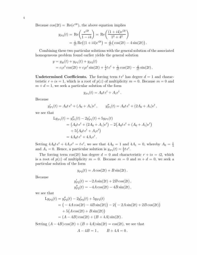
Because cos(2t) = Re(ei2t), the above equation implies

yP2(t) = Re

(

ei2t

1− i4

)

= Re

(

(1 + i4)ei2t

12 + 42

)

= 117Re

(

(1 + i4)ei2t)

= 117

(

cos(2t)− 4 sin(2t))

.

Combining these two particular solutions with the general solution of the associatedhomogeneous problem found earlier yields the general solution

y = yH(t) + yP1(t) + yP2(t)

= c1et cos(2t) + c2e

t sin(2t) + 14t et + 1

17cos(2t)− 4

17sin(2t) .

Undetermined Coefficients. The forcing term t et has degree d = 1 and charac-teristic r + is = 1, which is a root of p(z) of multiplicity m = 0. Because m = 0 andm+ d = 1, we seek a particular solution of the form

yP1(t) = A0t et + A1e

t .

Because

y′P1(t) = A0t et + (A0 + A1)e

t , y′′P1(t) = A0t et + (2A0 + A1)e

t ,

we see that

LyP1(t) = y′′P1(t)− 2y′P1(t) + 5yP1(t)

=(

A0t et + (2A0 + A1)e

t)

− 2(

A0t et + (A0 + A1)e

t)

+ 5(

A0t et + A1e

t)

= 4A0t et + 4A1e

t .

Setting 4A0t et + 4A1e

t = t et, we see that 4A0 = 1 and 4A1 = 0, whereby A0 = 14

and A1 = 0. Hence, a particular solution is yP1(t) =14t et.

The forcing term cos(2t) has degree d = 0 and characteristic r + is = i2, whichis a root of p(z) of multiplicity m = 0. Because m = 0 and m + d = 0, we seek aparticular solution of the form

yP2(t) = A cos(2t) +B sin(2t) .

Becausey′P2(t) = −2A sin(2t) + 2B cos(2t) ,

y′′P2(t) = −4A cos(2t)− 4B sin(2t) ,

we see that

LyP2(t) = y′′P2(t)− 2y′P2(t) + 5yP2(t)

=(

− 4A cos(2t)− 4B sin(2t))

− 2(

− 2A sin(2t) + 2B cos(2t))

+ 5(

A cos(2t) +B sin(2t))

= (A− 4B) cos(2t) + (B + 4A) sin(2t) .

Setting (A− 4B) cos(2t) + (B + 4A) sin(2t) = cos(2t), we see that

A− 4B = 1 , B + 4A = 0 .

5

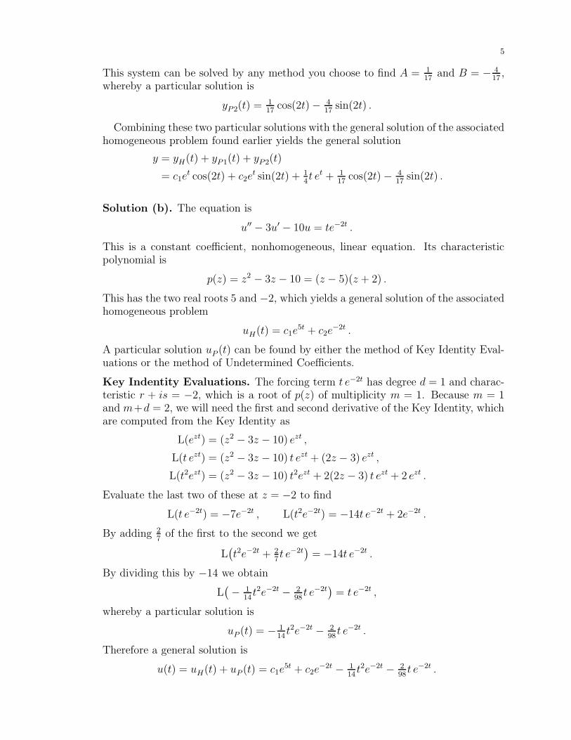
This system can be solved by any method you choose to find A = 117

and B = − 417,

whereby a particular solution is

yP2(t) =117cos(2t)− 4

17sin(2t) .

Combining these two particular solutions with the general solution of the associatedhomogeneous problem found earlier yields the general solution

y = yH(t) + yP1(t) + yP2(t)

= c1et cos(2t) + c2e

t sin(2t) + 14t et + 1

17cos(2t)− 4

17sin(2t) .

Solution (b). The equation is

u′′ − 3u′ − 10u = te−2t .

This is a constant coefficient, nonhomogeneous, linear equation. Its characteristicpolynomial is

p(z) = z2 − 3z − 10 = (z − 5)(z + 2) .

This has the two real roots 5 and −2, which yields a general solution of the associatedhomogeneous problem

uH(t) = c1e5t + c2e

−2t .

A particular solution uP (t) can be found by either the method of Key Identity Eval-uations or the method of Undetermined Coefficients.

Key Indentity Evaluations. The forcing term t e−2t has degree d = 1 and charac-teristic r + is = −2, which is a root of p(z) of multiplicity m = 1. Because m = 1and m+d = 2, we will need the first and second derivative of the Key Identity, whichare computed from the Key Identity as

L(ezt) = (z2 − 3z − 10) ezt ,

L(t ezt) = (z2 − 3z − 10) t ezt + (2z − 3) ezt ,

L(t2ezt) = (z2 − 3z − 10) t2ezt + 2(2z − 3) t ezt + 2 ezt .

Evaluate the last two of these at z = −2 to find

L(t e−2t) = −7e−2t , L(t2e−2t) = −14t e−2t + 2e−2t .

By adding 27of the first to the second we get

L(

t2e−2t + 27t e−2t

)

= −14t e−2t .

By dividing this by −14 we obtain

L(

− 114t2e−2t − 2

98t e−2t

)

= t e−2t ,


uP (t) = − 114t2e−2t − 2

98t e−2t .

Therefore a general solution is

u(t) = uH(t) + uP (t) = c1e5t + c2e

−2t − 114t2e−2t − 2

98t e−2t .

6

Undetermined Coefficients. The forcing term t e−2t has degree d = 1 and char-acteristic r + is = −2, which is a root of p(z) of multiplicity m = 1. Because m = 1and m+ d = 2, we seek a particular solution of the form

uP (t) = A0t2e−2t + A1t e

−2t .

Because

u′

P (t) = −2A0t2e−2t + (2A0 − 2A1)t e

−2t + A1e−2t ,

u′′

P (t) = 4A0t2e−2t + (−8A0 + 4A1)t e

−2t + (2A0 − 4A1)e−2t ,

we see that

LuP (t) = u′′

P (t)− 3u′

P (t)− 10uP (t)

=(

4A0t2e−2t + (−8A0 + 4A1)t e

−2t + (2A0 − 4A1)e−2t

)

− 3(

− 2A0t2e−2t + (2A0 − 2A1)t e

−2t + A1e−2t

)

− 10(

A0t2e−2t + A1t e

−2t)

= −14A0t e−2t + (2A0 − 7A1)e

−2t .

By setting −14A0t e−2t + (2A0 − 7A1)e

−2t = t e−2t we see that

−14A0 = 1 , 2A0 − 7A1 = 0 .

This system can be solved by any method you choose to find A0 = − 114

and A1 = − 298,


uP (t) = − 114t2e−2t − 2

98t e−2t .


u(t) = uH(t) + uP (t) = c1e5t + c2e

−2t − 114t2e−2t − 2

98t e−2t .

Solution (c). The equation is

v′′ + 9v = cos(3t) .

This is a constant coefficient, nonhomogeneous, linear equation. Its characteristicpolynomial is

p(z) = z2 + 9 = z2 + 32 .

This has the conjugate pair of roots ±i3, which yields a general solution of theassociated homogeneous problem

vH(t) = c1 cos(3t) + c2 sin(3t) .

A particular solution vP (t) can be found by either the method of Key Identity Eval-uations or the method of Undetermined Coefficients.

Key Indentity Evaluations. The forcing term cos(3t) has degree d = 0 andcharacteristic r + is = i3, which is a root of p(z) of multiplicity m = 1. Becausem = 1 and m+d = 1, we need the first derivative of the Key Identity, which is foundas

L(ezt) = (z2 + 9) ezt ,

L(t ezt) = (z2 + 9) t ezt + 2z ezt .

7

Evaluate the first derivative of the Key Identity at z = i3 to find that

L(t ei3t) = i6 ei3t .

Because cos(3t) = Re(ei3t), upon dividing by i6 and taking the real part we see thata particular solution is

vP (t) = Re(

1i6t ei3t

)

= Re(

1i6t (cos(3t) + i sin(3t))

)

= 16t sin(3t) .


v(t) = vH(t) + vP (t) = c1 cos(3t) + c2 sin(3t) +16t sin(3t) .

Undetermined Coefficients. The forcing term cos(3t) has degree d = 0 andcharacteristic r + is = i3, which is a root of p(z) of multiplicity m = 1. Becausem = 1 and m+ d = 1, we seek a particular solution of the form

vP (t) = At cos(3t) +Bt sin(3t) .

Because

v′P (t) = −3At sin(3t) + 3Bt cos(3t)A cos(3t) +B sin(3t) ,

v′′P (t) = −9At cos(3t)− 9Bt sin(3t)− 6A sin(3t) + 6B cos(3t) ,

we see that

LvP (t) = v′′P (t) + 9vP (t)

=(

− 9At cos(3t)− 9Bt sin(3t)− 6A sin(3t) + 6B cos(3t))

+ 9(

At cos(3t) +Bt sin(3t))

= −6A sin(3t) + 6B cos(3t) .

By setting −6A sin(3t)+6B cos(3t) = cos(3t) we see that A = 0 and B = 16, whereby

a particular solution is

vP (t) =16t sin(3t) .


v(t) = vH(t) + vP (t) = c1 cos(3t) + c2 sin(3t) +16t sin(3t) .

Remark. Because of the simple form of this equation, if we had tried to solve itby either the Green Function or Variation of Parameters method then integrals thatarise are not too difficult. However, it is not generally a good idea to use thesemethods for such problems because evaluating the integrals that arise often involvemuch more work that the methods shown above.

(5) Solve the following initial-value problems.(a) w′′ + 4w′ + 20w = 5e2t, w(0) = 3 , w′(0) = −7.

(b) y′′ − 4y′ + 4y =e2t

3 + t, y(0) = 0 , y′(0) = 5.

(c) tu′′ + 4u′ = 0, u(1) = 2 , u′(1) = −3.

8

Try to evaluate any definite integrals that arise.

Solution (a). This is a constant coefficient, nonhomogeneous, linear equation. Itscharacteristic polynomial is

p(z) = z2 + 4z + 20 = (z + 2)2 + 16 = (z + 2)2 + 42 .

This has the conjugate pair of roots −2 ± i4, which yields a general solution of theassociated homogeneous problem

wH(t) = c1e−2t cos(4t) + c2e

−2t sin(4t) .

A particular solution wP (t) can be found by either the method of Key Identity Eval-uations or the method of Undetermined Coefficients.

Key Indentity Evaluations. The forcing term 5e2t has degree d = 0 and charac-teristic r + is = 2, which is a root of p(z) of multiplicity m = 0. Because m = 0 andm+ d = 0, we only need the Key Identity,

L(ezt) = (z2 + 4z + 20) ezt .

Evaluate this at z = 2 to find that

L(e2t) = (4 + 8 + 20)e2t = 32e2t .

Upon multiplying this by 532

we see that a particular solution is

wP (t) =532e2t .

Undetermined Coefficients. The forcing term 5e2t has degree d = 0 and charac-teristic r+ is = 2, which is a root of p(z) of multiplicity m = 0. Therefore we seek aparticular solution of the form

wP (t) = Ae2t .

Becausew′

P (t) = 2Ae2t , w′′

P (t) = 4Ae2t ,

we see that

LwP (t) = w′′

P (t) + 4w′

P (t) + 20wP (t)

= 4Ae2t + 4(2Ae2t) + 20Ae2t = 32Ae2t .

By setting 32Ae2t = 5e2t, we see that A = 532, whereby a particular solution is

wP (t) =532e2t .

Solving the Initial-Value Problem. By either method we find that a generalsolution is

w(t) = wH(t) + wP (t) = c1e−2t cos(4t) + c2e

−2t sin(4t) + 532e2t .

Because

w′(t) = −2c1e−2t cos(4t)− 4c1e−2t sin(4t)

− 2c2e−2t sin(4t) + 4c2e

−2t cos(4t) + 516e2t ,

the initial conditions yield

3 = w(0) = c1 +532, −7 = w′(0) = −2c1 + 4c2 +

516.

9

Upon solving this system we find that c1 = 9132

and c2 = −1332, whereby the solution

of the initial-value problem is

w(t) = 9132e−2t cos(4t)− 13

32e−2t sin(4t) + 5

32e2t .

Solution (b). The initial-value problem is

y′′ − 4y′ + 4y =e2t

3 + t, y(0) = 0 , y′(0) = 5 .

This is a constant coefficient, nonhomogeneous, linear equation in normal form. Itscharacteristic polynomial is

p(z) = z2 − 4z + 4 = (z − 2)2 .

This has the double real root 2, which yields a general solution of the associatedhomogeneous problem

yH(t) = c1e2t + c2t e

2t .

A particular solution yP (t) cannot be found by either the method of Key IdentityEvaluations or the method of Undetermined Coefficients. Rather, we must use eitherthe Green Function or the Variation of Parameters method.

Green Function. The associated Green function g(t) satisfies

g′′ − 4g′ + 4g = 0 , g(0) = 0 , g′(0) = 1 .

A general solution of this equation is

g(t) = c1e2t + c2t e

2t .

Because 0 = g(0) = c1, we see that g(t) = c2t e2t. Then

g′(t) = c2e2t + 2c2t e

2t .

Because 1 = g′(0) = c2, the Green function is g(t) = t e2t. The particular solutionyP (t) that satisfies yP (0) = y′P (0) = 0 is given by

yP (t) =

∫ t

0

g(t− s)e2s

3 + sds =

∫ t

0

(t− s)e2t−2s e2s

3 + sds

= e2t∫ t

0

t− s

3 + sds = e2tt

∫ t

0

1

3 + sds− e2t

∫ t

0

s

3 + sds .

Because∫ t

0

1

3 + sds = log(3 + s)

∣

∣

∣

t

0= log(3 + t)− log(3) = log

(

3 + t

3

)

,

∫ t

0

s

3 + sds =

∫ t

0

1− 3

3 + sds = t− 3 log

(

3 + t

3

)

,

we find that

yP (t) = e2tt log(1 + 13t)− e2t

(

t− 3 log(1 + 13t))

.

Therefore a general solution of the equation is

y(t) = c1e2t + c2t e

2t + yP (t) .

10

Because

y′(t) = 2c1e2t + 2c2t e

2t + c2e2t + y′P (t) ,

and because yP (0) = y′P (0) = 0, the initial conditions imply

0 = y(0) = c1 , 5 = y′(0) = 2c1 + c2 .

We find that c1 = 0 and c2 = 5, whereby the solution of the initial-value problem is

y(t) = 5t e2t + e2tt log(1 + 13t)− e2t

(

t− 3 log(1 + 13t))

.

Variation of Parameters. The equation is already in normal form. Therefore weseek a particular solution of the form

yP (t) = e2tu1(t) + t e2tu2(t) ,

such thate2tu′

1(t) + t e2tu′

2(t) = 0 ,

2e2tu′

1(t) + (2t e2t + e2t)u′

2(t) =e2t

3 + t.

This system can be solved to find that

u′

1(t) = −t

3 + t, u′

2(t) =1

3 + t.

These can be integrted to obtain

u1(t) = −∫

t

3 + tdt = −

∫

1− 3

3 + tdt = −t+ 3 log(3 + t) + c1 ,

u2(t) =

∫

1

3 + tdt = log(3 + t) + c2 ,

whereby a general solution is

y(t) = c1e2t − e2t

(

t− 3 log(3 + t))

+ c2t e2t + t e2t log(3 + t) .

Because

y′(t) = 2c1e2t − 2e2t

(

t− 3 log(3 + t))

− e2t(

1− 3

3 + t

)

+ 2c2t e2t + c2e

2t + 2t e2t log(3 + t) + e2t log(3 + t) + t e2t1

3 + t,

the initial conditions imply that

0 = y(0) = c1 + 3 log(3) ,

5 = y′(0) = 2c1 + 6 log(3) + c2 + log(3) .

We can solve this system to find that c1 = −3 log(3) and c2 = 5 − log(3). Thereforethe solution of the initial-value problem is

y(t) = −3 log(3)e2t − e2t(

t− 3 log(3 + t))

+(

5− log(3))

t e2t + t e2t log(3 + t) .

Solution (c). The initial-value problem is

tu′′ + 4u′ = 0 , u(1) = 2 , u′(1) = −3 .

11

This is a variable coefficient, homogeneous, second-order linear equation. Because itdoes not depend explictly on u, we can reduce its order by setting w = u′. Then w

satisfies the initial-value problem

tw′ + 4w = 0 , w(1) = −3 .This is a variable coefficient, homogeneous, first-order linear equation. Its normalform is

w′ +4

tw = 0 , w(1) = −3 .

By setting

A(t) =

∫ t

1

4

sds = 4 log(s)

∣

∣

∣

t

1= 4 log(t)− 4 log(1) = 4 log(t) ,

the solution of the initial-value problem for w is

w(t) = w(1)e−A(t) = −3e−4 log(t) = −3t−4 .

Then because u′ = w and u(1) = 2 we see that

u(t) = u(1) +

∫ t

1

w(s) ds = 2− 3

∫ t

1

s−4 ds = 2 +[

s−3]

∣

∣

∣

t

1= 2 + t−3 − 1 = 1 + t−3 .

The interval of definition for this solution is (0,∞), which can be seen by putting theoriginal initial-value problem into normal form.

(6) Give an explicit general solution of the equation

h′′ + 2h′ + 5h = 0 .

Sketch a typical solution for t ≥ 0. If this equation governs a spring-mass system, isthe system undamped, under damped, critically damped, or over damped?

Solution. This is a constant coefficient, homogeneous, linear equation. Its charac-teristic polynomial is

p(z) = z2 + 2z + 5 = (z + 1)2 + 22 .

This has the conjugate pair of roots −1± i2, which yields a general solution

h(t) = c1e−t cos(2t) + c2e

−t sin(2t) .

When c 21 + c 2

2 > 0 this can be put into the amplitute-phase form

h(t) = Ae−t cos(2t− δ) ,

where A > 0 and 0 ≤ δ < 2π are determined from c1 and c2 by

A =√

c 21 + c 2

2 , cos(δ) =c1

A, sin(δ) =

c2

A.

In other words, (A, δ) are the polar coordinates for the point in the plane whoseCartesian coordinates are (c1, c2). The sketch should show a decaying oscillationwith amplitude Ae−t and quasiperiod 2π

2= π. A sketch might be given during the

review session. The equation governs an under damped spring-mass system becauseits characteristic polynomial has a conjugate pair of roots with negative real part.

12

(7) When a mass of 2 kilograms is hung vertically from a spring, it stretches the spring0.5 meters. (Gravitational acceleration is 9.8 m/sec2.) At t = 0 the mass is set inmotion from 0.3 meters below its equilibrium (rest) position with a upward velocity of2 m/sec. It is acted upon by an external force of 2 cos(5t). Neglect drag and assumethat the spring force is proportional to its displacement. Formulate an initial-valueproblem that governs the motion of the mass for t > 0. (DO NOT solve this initial-value problem; just write it down!)

Solution. Let h(t) be the displacement (in meters) of the mass from its equilibrium(rest) position at time t (in seconds), with upward displacements being positive. Thegoverning initial-value problem then has the form

md2h

dt2+ kh = 2 cos(5t) , h(0) = −.3 , h′(0) = 2 ,

where m is the mass and k is the spring constant. The problem says that m = 2kilograms. The spring constant is obtained by balancing the weight of the mass (mg

= 2 · 9.8 Newtons) with the force applied by the spring when it is stetched .5 m.This gives k .5 = 2 · 9.8, or

k =2 · 9.8.5

= 4 · 9.8 Newtons/m .

Therefore the governing initial-value problem is

2d2h

dt2+ 4 · 9.8h = 2 cos(5t) , h(0) = −.3 , h′(0) = 2 .

Had you chosen downward displacements to be positive then the sign of the initialdata would change! You should make your convention clear!

(8) Find the Laplace transform Y (s) of the solution y(t) to the initial-value problem

y′′ + 4y′ + 8y = f(t) , y(0) = 2 , y′(0) = 4 .

where

f(t) =

{

4 for 0 ≤ t < 2 ,

t2 for 2 ≤ t .

You may refer to the table of Laplace transforms on the last page. (DO NOT takethe inverse Laplace transform to find y(t); just solve for Y (s)!)

Solution. The Laplace transform of the initial-value problem is

L[y′′](s) + 4L[y′](s) + 8L[y](s) = L[f ](s) ,where

L[y](s) = Y (s) ,

L[y′](s) = sY (s)− y(0) = sY (s)− 2 ,

L[y′′](s) = s2Y (s)− sy(0)− y′(0) = s2Y (s)− 2s− 4 .

To compute L[f ](s), first write f as

f(t) =(

1− u(t− 2))

4 + u(t− 2)t2 = 4− u(t− 2)4 + u(t− 2)t2

= 4 + u(t− 2)(t2 − 4) = 4 + u(t− 2)j(t− 2) ,

13

wherej(t) = (t+ 2)2 − 4 = t2 + 4t .

Referring to the table of Laplace transforms, line 1, line 13 with c = 2, and line 3with n = 1 and n = 2 then show that

L[f ](s) = 4L[1](s) + L[

u(t− 2)j(t− 2)]

(s)

= 4L[1](s) + e−2sL[

j(t)]

(s)

= 4L[1](s) + e−2sL[4t+ t2](s)

= 4L[1](s) + 4e−2sL[t](s) + e−2sL[t2](s)

= 41

s+ 4e−2s 1

s2+ e−2s 2

s3.

The Laplace transform of the initial-value problem then becomes

(

s2Y (s)− 2s− 4)

+ 4(

sY (s)− 2)

+ 8Y (s) =4

s+ e−2s 4

s2+ e−2s 2

s3,

which becomes

(s2 + 4s+ 8)Y (s)− 2s− 12 =4

s+ e−2s 4

s2+ e−2s 2

s3.

Hence, Y (s) is given by

Y (s) =1

s2 + 4s+ 8

(

2s+ 12 +4

s+ e−2s 4

s2+ e−2s 2

s3

)

.

(9) Find the function y(t) whose Laplace transform Y (s) is given by

(a) Y (s) =e−3s4

s2 − 6s+ 5, (b) Y (s) =

e−2ss

s2 + 4s+ 8.

You may refer to the table of Laplace transforms on the last page.

Solution (a). The denominator factors as (s − 5)(s − 1), so we have the partialfraction identity

4

s2 − 6s+ 5=

4

(s− 5)(s− 1)=

1

s− 5− 1

s− 1.

Referring to the table of Laplace transforms, line 2 with a = 5 and with a = 1 gives

L−1

[

1

s− 5

]

(t) = e5t , L−1

[

1

s− 1

]

(t) = et ,

whereby

L−1

[

4

s2 − 6s+ 5

]

(t) = L−1

[

1

s− 5− 1

s− 1

]

= e5t − et .

It follows from line 13 with c = 3 and j(t) = e5t − et that

y(t) = L−1[Y (s)](t) = L−1

[

e−3s4

s2 − 6s+ 5

]

(t)

= u(t− 3)L−1

[

4

s2 − 6s+ 5

]

(t− 3) = u(t− 3)(

e5(t−3) − et−3)

.

14

Solution (b). The denominator does not have real factors. The partial fractionidentity is

s

s2 + 4s+ 8=

s

(s+ 2)2 + 4=

s + 2

(s+ 2)2 + 22− 2

(s+ 2)2 + 22.

Referring to the table of Laplace transforms, lines 8 and 7 with a = −2 and b = 2give

L−1

[

s+ 2

(s+ 2)2 + 22

]

(t) = e−2t cos(2t) , L−1

[

2

(s+ 2)2 + 22

]

(t) = e−2t sin(2t) ,

whereby

L−1

[

s

s2 + 4s+ 8

]

(t) = L−1

[

s + 2

(s+ 2)2 + 22

]

(t)− L−1

[

2

(s+ 2)2 + 22

]

(t)

= e−2t(

cos(2t)− sin(2t))

.

It follows from line 13 with c = 2 and j(t) = e−2t(

cos(2t)− sin(2t))

that

y(t) = L−1[Y (s)](t) = L−1

[

e−2ss

s2 + 4s+ 8

]

(t) = u(t− 2)L−1

[

s

s2 + 4s+ 8

]

(t− 2)

= u(t− 2)e−2(t−2)(

cos(2(t− 2))− sin(2(t− 2)))

.

(10) Consider two interconnected tanks filled with brine (salt water). The first tankcontains 80 liters and the second contains 30 liters. Brine flows with a concentrationof 3 grams of salt per liter flows into the first tank at a rate of 2 liters per hour. Wellstirred brine flows from the first tank to the second at a rate of 6 liters per hour,from the second to the first at a rate of 4 liters per hour, and from the second into adrain at a rate of 2 liters per hour. At t = 0 there are 7 grams of salt in the first tankand 25 grams in the second. Give an initial-value problem that governs the amountof salt in each tank as a function of time.

Solution: The rates work out so there will always be 80 liters of brine in the firsttank and 30 liters in the second. Let S1(t) be the grams of salt in the first tank andS2(t) be the grams of salt in the second tank. These are governed by the initial-valueproblem

dS1

dt= 3·2 + S2

304− S1

806 , S1(0) = 7 ,

dS2

dt=

S1

806− S2

304− S2

302 , S2(0) = 25 .

You could leave the answer in the above form. It can however be simplified to

dS1

dt= 6 + 2

15S2 − 3

40S1 , S1(0) = 7 ,

dS2

dt= 3

40S1 − 1

5S2 , S2(0) = 25 .

(11) Consider the real vector-valued functions x1(t) =

(

1t

)

, x2(t) =

(

t3

3 + t4

)

.

(a) Compute the Wronskian W [x1,x2](t).

15

(b) Suppose that x1 and x2 comprise a fundamental set of solutions to the linearsystem x′ = A(t)x. Give a general solution to this system.

Solution (a). The Wronskian is given by

W [x1,x2](t) = det

(

1 t3

t 3 + t4

)

= 1 · (3 + t4)− t · t3 = 3 + t4 − t4 = 3 .

Solution (b). Because x1(t), x2(t) is a fundamental set of solutions for the linearsystem whose coefficient matrix is A(t), a general solution is given by

x(t) = c1x1(t) + c2x2(t) = c1

(

1t

)

+ c2

(

t3

3 + t4

)

.

(12) Give a general real vector-valued solution of the linear planar system x′ = Ax for

(a) A =

(

6 44 0

)

, (b) A =

(

1 2−2 1

)

.

Solution (a). The characteristic polynomial of A is

p(z) = z2 − tr(A)z + det(A)

= z2 − 6z − 16 = (z − 3)2 − 25 = (z − 3)2 − 52 .

The eigenvalues of A are the roots of this polynomial, which are 3± 5, or simply −2and 8. Therefore we have

etA = e3t[

cosh(5t)I+sinh(5t)

5(A− 3I)

]

= e3t[

cosh(5t)

(

1 00 1

)

+sinh(5t)

5

(

3 44 −3

)]

= e3t(

cosh(5t) + 35sinh(5t) 4

5sinh(5t)

45sinh(5t) cosh(5t)− 3

5sinh(5t)

)

.

Therefore a general solution is given by

x(t) = etA(

c1c2

)

= c1e3t

(

cosh(5t) + 35sinh(5t)

45sinh(5t)

)

+ c2e3t

(

45sinh(5t)

cosh(5t)− 35sinh(5t)

)

.

Alternative Solution (a). The characteristic polynomial of A is


= z2 − 6z − 16 = (z − 3)2 − 25 = (z − 3)2 − 52 .

The eigenvalues of A are the roots of this polynomial, which are 3± 5, or simply −2and 8. Because

A+ 2I =

(

8 44 2

)

, A− 8I =

(

−2 44 −8

)

,

we see that A has the eigenpairs(

−2 ,(

1−2

))

,

(

8 ,

(

21

))

.

16

Form these eigenpairs we construct the solutions

x1(t) = e−2t

(

1−2

)

, x2(t) = e8t(

21

)

,


x(t) = c1x1(t) + c2x2(t) = c1e−2t

(

1−2

)

+ c2e8t

(

21

)

.

Solution (b). The characteristic polynomial of A is


= z2 − 2z + 5 = (z − 1)2 + 4 = (z − 1)2 + 22 .

The eigenvalues of A are the roots of this polynomial, which are 1 ± i2. Thereforewe have

etA = et[

cos(2t)I+sin(2t)

2(A− I)

]

= et[

cos(2t)

(

1 00 1

)

+sin(2t)

2

(

0 2−2 0

)]

= et(

cos(2t) sin(2t)− sin(2t) cos(2t)

)

.

Therefore a general solution is given by

x(t) = etA(

c1c2

)

= c1et

(

cos(2t)− sin(2t)

)

+ c2et

(

sin(2t)cos(2t)

)

.

Alternative Solution (b). The characteristic polynomial of A is


= z2 − 2z + 5 = (z − 1)2 + 4 = (z − 1)2 + 22 .

The eigenvalues of A are the roots of this polynomial, which are 1± i2. Because

A− (1 + i2)I =

(

−i2 2−2 −i2

)

, A− (1− i2)I =

(

i2 2−2 i2

)

,

we see that A has the eigenpairs(

1 + i2 ,

(

1i

))

,

(

1− i2 ,

(

−i1

))

.

Because

e(1+i2)t

(

1i

)

= et(

cos(2t) + i sin(2t)− sin(2t) + i cos(2t)

)

,

two real solutions of the system are

x1(t) = et(

cos(2t)− sin(2t)

)

, x2(t) = et(

sin(2t)cos(2t)

)

.


x(t) = c1x1(t) + c2x2(t) = c1et

(

cos(2t)− sin(2t)

)

+ c2et

(

sin(2t)cos(2t)

)

.

17

(13) What answer will be produced by the following Matlab command?

>> A = [1 4; 3 2]; [vect, val] = eig(sym(A))

You do not have to give the answer in Matlab format.

Solution. The Matlab command will produce the eigenpairs of A =

(

1 43 2

)

. The

characteristic polynomial of A is

p(z) = z2 − tr(A)z + det(A) = z2 − 3z − 10 = (z − 5)(z + 2) ,

so its eigenvalues are 5 and −2. Because

A− 5I =

(

−4 43 −3

)

, A+ 2I =

(

3 43 4

)

,

we can read off that the eigenpairs are(

5 ,

(

11

))

,

(

−2 ,(

−43

))

.

(14) A real 2×2 matrix A has eigenvalues 2 and −1 with associated eigenvectors(

31

)

and

(

−12

)

.

(a) Give a general solution to the linear planar system x′ = Ax.(b) Compute etA.(c) Sketch a phase-plane portrait for this system and identify its type. Classify the

stability of the origin. Carefully mark all sketched orbits with arrows!

Solution (a). Use the given eigenpairs to construct the solutions

x1(t) = e2t(

31

)

, x2(t) = e−t

(

−12

)

.


x(t) = c1x1(t) + c2x2(t) = c1e2t

(

31

)

+ c2e−t

(

−12

)

.

Solution (b). The matrix A can be diagonalized as A = VDV−1 where

V =

(

3 −11 2

)

, D =

(

2 00 −1

)

, V−1 =1

7

(

2 1−1 3

)

.

Then

etA = VetDV−1 =1

7

(

3 −11 2

)(

e2t 00 e−t

)(

2 1−1 3

)

=1

7

(

3e2t −e−t

e2t 2e−t

)(

2 1−1 3

)

=1

7

(

6e2t + e−t 3e2t − 3e−t

2e2t − 2e−t e2t + 6e−t

)

.

18

Alternative Solution (b). By part (a) a fundamental matrix is

Ψ(t) =(

x1(t) x2(t))

=

(

3e2t −e−t

e2t 2e−t

)

.

Then

etA = Ψ(t)Ψ(0)−1 =

(

3e2t −e−t

e2t 2e−t

)(

3 −11 2

)

−1

=1

7

(

3e2t −e−t

e2t 2e−t

)(

2 1−1 3

)

=1

7

(

6e2t + e−t 3e2t − 3e−t

2e2t − 2e−t e2t + 6e−t

)

.

Solution (c). The matrix A has two real eigenvalues of opposite sign. Therefore theorigin is a saddle and is thereby unstable. There is one orbit moves away from (0, 0)along each half of the line x = 3y, and one orbit moves towards (0, 0) along each halfof the line y = −2x. (These are the lines of eigenvectors.) Every other orbit sweepsaway from the line y = −2x and towards the line x = 3y. A phase-plane portraitmight be sketched during the review session.

(15) Solve the initial-value problem x′ = Ax, x(0) = xI and describe how its solutionbehaves as t→∞ for the following A and xI .

(a) A =

(

3 10−5 −7

)

, xI =

(

−32

)

.

(b) A =

(

8 −55 −2

)

, xI =

(

3−1

)

.

Solution (a). The characteristic polynomial of A =

(

3 10−5 −7

)

is

p(z) = z2 − tr(A)z + det(A) = z2 + 4z + 29 = (z + 2)2 + 52 .

Therefore the eigenvlues of A are −2 ± i5. Then

etA = e−2t

[

cos(5t)I+sin(5t)

5(A+ 2I)

]

= e−2t

[

cos(5t)

(

1 00 1

)

+sin(5t)

5

(

5 10−5 −5

)]

= e−2t

(

cos(5t) + sin(5t) 2 sin(5t)− sin(5t) cos(5t)− sin(5t)

)

.

Therefore the solution of the initial-value problem is

x(t) = etAxI = e−2t

(


)(

−32

)

= e−2t

(

−3 cos(5t) + sin(5t)2 cos(5t) + sin(5t)

)

.

This solution decays to zero as t→∞.

19

Alternative Solution (a). The characteristic polynomial of A =

(

3 10−5 −7

)

is

p(z) = z2 − tr(A)z + det(A) = z2 + 4z + 29 = (z + 2)2 + 52 .

Therefore the eigenvlues of A are −2 ± i5. Because

A− (−2 + i5)I =

(

5− i5 10−5 −5− i5

)

,

we can read off that A has the conjugate eigenpairs(

−2 + i5 ,

(

1 + i

−1

))

,

(

−2 − i5 ,

(

1− i

−1

))

.

Because

e−2t+i5t

(

1 + i

−1

)

= e−2t(

cos(5t) + i sin(5t))

(

1 + i

−1

)

= e−2t

(

cos(5t)− sin(5t) + i cos(5t) + i sin(5t)− cos(5t)− i sin(5t)

)

,

a fundamental set of real solutions is

x1(t) = e−2t

(

cos(5t)− sin(5t)− cos(5t)

)

, x2(t) = e−2t

(

cos(5t) + sin(5t)− sin(5t)

)

.

Then a fundamental matrix Ψ(t) is given by

Ψ(t) =(

x1(t) x2(t))

= e−2t

(

cos(5t)− sin(5t) cos(5t) + sin(5t)− cos(5t) − sin(5t)

)

.

Because

Ψ(0)−1 =

(

1 1−1 0

)

−1

=1

1

(

0 −11 1

)

=

(

0 −11 1

)

,

we see that

etA = Ψ(t)Ψ(0)−1 = e−2t

(

cos(5t)− sin(5t) cos(5t) + sin(5t)− cos(5t) − sin(5t)

)(

0 −11 1

)

= e−2t

(


)

.


x(t) = etAxI = e−2t

(


)(

−32

)

= e−2t

(

−3 cos(5t) + sin(5t)2 cos(5t) + sin(5t)

)

.

This solution decays to zero as t→∞.

Remark. After we have constructed the fundmental set of solutions x1(t) and x2(t),we could also have solved the initial-value problem by finding constants c1 and c2such that x(t) = c1x1(t) + c2x2(t) satisfies the initial condition. Had we done thisusing the x1(t) and x2(t) constructed above, we would have found that c1 = −2 andc2 = −1.

20

Solution (b). The characteristic polynomial of A =

(

8 −55 −2

)

is

p(z) = z2 − tr(A)z + det(A) = z2 − 6z + 9 = (z − 3)2 .

The ony eigenvalue of A is 3. Then

etA = e3t[

I+ t (A− 3I)]

= e3t[(

1 00 1

)

+ t

(

5 −55 −5

)]

= e3t(

1 + 5t −5t5t 1− 5t

)

.


x(t) = etAxI = e3t(

1 + 5t −5t5t 1− 5t

)(

3−1

)

= e3t(

3 + 20t−1 + 20t

)

.

This solution grows like 20t e3t as t→∞.

Alternative Solution (b). The characteristic polynomial of A =

(

8 −55 −2

)

is

p(z) = z2 − tr(A)z + det(A) = z2 − 6z + 9 = (z − 3)2 .

The only eigenvalue of A is 3. Because

A− 3I =

(

5 −55 −5

)

,

we can read off that A has the eigenpair(

3 ,

(

11

))

.

We can use this eigenpair to construct the solution

x1(t) = e3t(

11

)

.

A second solution can be constructed by

x2(t) = e3tw + t e3t(A− 3I)w ,

where w is any nonzero vector that is not an eigenvector associated with 3. For

example, taking w =(

1 0)T

yields

x2(t) = e3t(

10

)

+ t e3t(

5 −55 −5

)(

10

)

= e3t(

1 + 5t5t

)

.

Then a fundamental matrix Ψ(t) is given by

Ψ(t) =(

x1(t) x2(t))

= e3t(

1 1 + 5t1 5t

)

.

Because

Ψ(0)−1 =

(

1 11 0

)

−1

=1

−1

(

0 −1−1 1

)

=

(

0 11 −1

)

,

21

we see that

etA = Ψ(t)Ψ(0)−1 =

(

1 1 + 5t1 5t

)(

0 11 −1

)

=

(

1 + 5t −5t5t 1− 5t

)

.


x(t) = etAxI = e3t(

1 + 5t −5t5t 1− 5t

)(

3−1

)

= e3t(

3 + 20t−1 + 20t

)

.

This solution grows like 20t e3t as t→∞.

Remark. After we have constructed the fundmental set of solutions x1(t) and x2(t),we could also have solved the initial-value problem by finding constants c1 and c2such that x(t) = c1x1(t) + c2x2(t) satisfies the initial condition. Had we done thisusing the x1(t) and x2(t) constructed above, we would have found that c1 = −1 andc2 = 4.

(16) Consider the nonlinear planar system

x′ = 2xy ,

y′ = 9− 9x− y2 .

(a) Find all of its stationary points.(b) Find a nonconstant function H(x, y) such that every orbit of the system satisfies

H(x, y) = c for some constant c.(c) Classify the type and stability of each stationary point.(d) Sketch the level sets (contour lines) H(x, y) = c for values of c corresponding to

each saddle point. Use arrows to indicate the direction of the orbit along eachcurve that you sketch!

Solution (a). Stationary points satisfy

0 = 2xy ,

0 = 9− 9x− y2 .

The top equation shows that x = 0 or y = 0. If x = 0 then the bottom equationbecomes 0 = 9 − y2 = (3 − y)(3 + y), which shows that either y = 3 or y = −3. Ify = 0 then the bottom equation becomes 0 = 9 − 9x = 9(1 − x), which shows thatx = 1. Therefore the stationary points of the system are

(0, 3) , (0,−3) , (1, 0) .

Solution (b). The associated first-order orbit equation is

dy

dx=

9− 9x− y2

2xy.

This equation is not linear or separable. It has the differential form

(y2 + 9x+−9) dx+ 2xy dy = 0 ,

which is exact because

∂y(y2 + 9x− 9) = 2y = ∂x(2xy) = 2y .

22

Therefore there exists H(x, y) such that

∂xH(x, y) = y2 + 9x− 9 , ∂yH(x, y) = 2xy .

By integrating the second equation we see that

H(x, y) = xy2 + h(x) .

When this is substituted into the first equation we find

∂xH(x, y) = y2 + h′(x) = y2 + 9x− 9 ,

which implies that h′(x) = 9x− 9. By taking h(x) = 92x2 − 9x we obtain

H(x, y) = xy2 + 92x2 − 9x .

Alternative Solution (b). Notice that

∂xf(x, y) + ∂yg(x, y) = ∂x(2xy) + ∂y(9− 9x− y2) = 2y − 2y = 0 .

Therefore the system has Hamiltonian form with Hamiltonian H(x, y) that satisfies

∂yH(x, y) = 2xy , −∂xH(x, y) = 9− 9x− y2 .

By integrating the first equation we see that

H(x, y) = xy2 + h(x) .

When this is substituted into the second equation we find

−∂xH(x, y) = −y2 − h′(x) = 9− 9x− y2 ,

which implies that h′(x) = 9x− 9. By taking h(x) = 92x2 − 9x we obtain

H(x, y) = xy2 + 92x2 − 9x .

Solution (c). Because

f(x, y) =

(

f(x, y)g(x, y)

)

=

(

2xy9− 9x− y2

)

,

the Jacobian matrix ∂f(x, y) of partial derivatives is

∂f(x, y) =

(

∂xf(x, y) ∂yf(x, y)∂xg(x, y) ∂yg(x, y)

)

=

(

2y 2x−9 −2y

)

.

Evaluating this matrix at each stationary point yields

∂f(0, 3) =

(

6 0−9 −6

)

, ∂f(0,−3) =(

−6 0−9 6

)

, ∂f(1, 0) =

(

0 2−9 0

)

.

• Because the matrix ∂f(0, 3) is lower triangular, we can read off that its eigen-values are 6 and −6. Because these are real with opposite signs, the stationarypoint (0, 3) is a saddle and thereby is unstable.

• Because the matrix ∂f(0,−3) is lower triangular, we can read off that its eigen-values are −6 and 6. Because these are real with opposite signs, the stationarypoint (0,−3) is a saddle and thereby is unstable.

23

• The characteristic polynomial of the matrix ∂f(1, 0) is

p(z) = z2 + 18 ,

so the matrix ∂f(1, 0) has eigenvalues ±i√18. Because these are immaginary

and the system has an integral while the lower left entry of ∂f(1, 0) is negative,the stationary point (1, 0) is a clockwise center and thereby is stable.

Alternative Solution (c). If you saw that the system has Hamiltonian form withHamiltonian H(x, y) from part (b) then you can take this approach. The Hessianmatrix ∂

2H(x, y) of second partial derivatives of the Hamiltonian H(x, y) is

∂2H(x, y) =

(

∂xxH(x, y) ∂xyH(x, y)∂yxH(x, y) ∂yyH(x, y)

)

=

(

9 2y2y 2x

)

.

Evaluating this at the stationary points yields

∂2H(0, 3) =

(

9 66 0

)

, ∂2H(0,−3) =

(

9 −6−6 0

)

, ∂2H(1, 0) =

(

9 00 2

)

.

• The characteristic polynomial of the matrix ∂2H(0, 3) is

p(z) = z2 − 9z − 36 = (z − 12)(z + 3) .

Therefore the matrix ∂2H(0, 3) has eigenvalues 12 and −3. Because these have

different signs, the stationary point (0, 3) is a saddle and thereby is unstable.

• The characteristic polynomial of the matrix ∂2H(0,−3) is

p(z) = z2 − 9z − 36 = (z − 12)(z + 3) .

Therefore the matrix ∂2H(0,−3) has eigenvalues 12 and −3. Because these have

different signs, the stationary point (0,−3) is a saddle and thereby is unstable.

• Because the matrix ∂2H(1, 0) is diagonal, we can read off that its eigenvalues

are 9 and 2. Because these are both positive, the stationary point (1, 0) is aclockwise center and thereby is stable.

Solution (d). The saddle points are (0, 3) and (0,−3). BecauseH(0, 3) = H(0,−3) = 0 · (±3)2 + 9

2· 02 − 9 · 0 = 0 .

Hence, the level set corresponding to these saddle points is

0 = xy2 + 92x2 − 9x = (y2 + 9

2x− 9)x .

The points on this set must satisfy either y2 + 92x − 9 = 0 or x = 0. Therefore the

level set is the union of the parabola x = 2− 29y2 and the y-axis.

Along the y-axis (x = 0) the y′ equation reduces to y′ = 9 − y2 = (3 − y)(3 + y),whereby the arrows point towards (0, 3) and away from (0,−3). Along the parabolax = 2− 2

9y2 the arrows point away from (0, 3) and towards (0,−3) because they are

saddle points.

24


x′ = −5y ,y′ = x− 4y − x2 .

(a) Find all of its stationary points.(b) Compute the Jacobian matrix at each stationary point.(c) Classify the type and stability of each stationary point.(d) Sketch a plausible global phase-plane portrait. Use arrows to indicate the direc-

tion of the orbit along each curve that you sketch!


0 = −5y , 0 = x− 4y − x2 .

The first equation implies y = 0, whereby the second equation becomes 0 = x−x2 =x(1− x), which implies either x = 0 or x = 1. Therefore all the stationary points ofthe system are

(0, 0) , (1, 0) .

Solution (b). Because

f(x, y) =

(

f(x, y)g(x, y)

)

=

(

−5yx− 4y − x2

)

,

the Jacobian matrix of partial derivatives is

∂f(x, y) =

(


)

=

(

0 −51− 2x −4

)

.

Evaluating this matrix at each stationary point yields the coefficient matrices

A =

(

0 −51 −4

)

at (0, 0) , A =

(

0 −5−1 −4

)

at (1, 0) .

Solution (c). The coefficient matrix A at (0, 0) has eigenvalues that satisfy

0 = det(zI −A) = z2 − tr(A)z + det(A) = z2 + 4z + 5 = (z + 2)2 + 12 .

The eigenvalues are thereby −2± i. Because a21 = 1 > 0, the stationary point (0, 0)is a counterclockwise spiral sink, which is attracting. This is one of the generic types,so it describes the phase-plane portrait of the nonlinear system near (0, 0).The coefficient matrix A at (1, 0) has eigenvalues that satisfy

0 = det(zI−A) = z2 − tr(A)z + det(A) = z2 + 4z − 5 = (z + 2)2 − 32 .

The eigenvalues are thereby −2± 3, or simply −5 and 1. The stationary point (1, 0)is thereby a saddle, which is unstable. This is one of the generic types, so it describesthe phase-plane portrait of the nonlinear system near (1, 0).

Solution (d). The nullcline for x′ is the line y = 0. This line partitions the planeinto regions where x is increasing or decreasing as t increases. The nullcline for y′ isthe parabola y = 1

4(x − x2). This curve partitions the plane into regions where y is

increasing or decreasing as t increases. Neither of these nullclines is invariant.

The stationary point (0, 0) is a counterclockwise spiral sink.

25

The stationary point (1, 0) is a saddle. The coefficient matrix A has eigenvalues−5 and 1. Because

A+ 5I =

(

5 −5−1 1

)

, A− I =

(

−1 −5−1 −5

)

,

it has the eigenpairs(

−5 ,(

11

))

,

(

1 ,

(

−51

))

Near (1, 0) there is one orbit that emerges from (1, 0) tangent to each side of the linex = 1− 5y. There is also one orbit that approaches (1, 0) tangent to each side of theline y = x− 1. These orbits are separatrices. A global phase-plane portrait might besketched during the review session.

Remark. The global phase-plane portrait becomes clearer if we had seen thatH(x, y) = 1

2x2 + 5

2y2 − 1

3x3 satisfies

d

dtH(x, y) = ∂xH(x, y) x′ + ∂yH(x, y) y′

= (x− x2)(−5y) + 5y(x− 4y − x2) = −20y2 ≤ 0 .

The orbits of the system are thereby seen to cross the contour lines of H(x, y) so asto decrease H(x, y). You would not be expected to see this on the Final Exam.


x′ = x(3− 3x+ 2y) ,

y′ = y(6− x− y) .

Do parts (a-d) as for the previous problem.(e) Why do solutions that start in the first quadrant stay in the first quadrant?


0 = x(3− 3x+ 2y) , 0 = y(6− x− y) .

The first equation implies either x = 0 or 3− 3x+2y = 0, while the second equationimplies either y = 0 or 6 − x− y = 0. If x = 0 and y = 0 then (0, 0) is a stationarypoint. If x = 0 and 6− x− y = 0 then (0, 6) is a stationary point. If 3− 3x+2y = 0and y = 0 then (1, 0) is a stationary point. If 3− 3x+2y = 0 and 6− x− y = 0 thenupon solving these equations we find that (3, 3) is a stationary point. Therefore allthe stationary points of the system are

(0, 0) , (0, 6) , (1, 0) , (3, 3) .

Solution (b). Because

f(x, y) =

(

f(x, y)g(x, y)

)

=

(

3x− 3x2 + 2xy6y − xy − y2

)

,

the Jacobian matrix of partial derivatives is

∂f(x, y) =

(


)

=

(

3− 6x+ 2y 2x−y 6− x− 2y

)

.

26

Evaluating this matrix at each stationary point yields the coefficient matrices

A =

(

3 00 6

)

at (0, 0) ,

A =

(

−3 20 5

)

at (1, 0) ,

A =

(

15 0−6 −6

)

at (0, 6) ,

A =

(

−9 6−3 −3

)

at (3, 3) .

Solution (c). The coefficient matrix A at (0, 0) is diagonal, so we can read-off itseigenvalues as 3 and 6. The stationary point (0, 0) is thereby a nodal source, whichis repelling. This is one of the generic types, so it describes the phase-plane portraitof the nonlinear system near (0, 0).

The coefficient matrix A at (0, 6) is triangular, so we can read-off its eigenvaluesas −6 and 15. The stationary point (0, 6) is thereby a saddle, which is unstable. Thisis one of the generic types, so it describes the phase-plane portrait of the nonlinearsystem near (0, 6).

The coefficient matrix A at (1, 0) is triangular, so we can read-off its eigenvaluesas −3 and 5. The stationary point (1, 0) is thereby a saddle, which is unstable. Thisis one of the generic types, so it describes the phase-plane portrait of the nonlinearsystem near (1, 0).The coefficient matrix A at (3, 3) has eigenvalues that satisfy

0 = det(zI −A) = z2 − tr(A)z + det(A) = z2 + 12z + 45 = (z + 6)2 + 32 .

Its eigenvalues are thereby −6 ± i3. Because a21 = −3 < 0, the stationary point(3, 3) is a clockwise spiral sink, which is attracting. This is one of the generic types,so it describes the phase-plane portrait of the nonlinear system near (3, 3).

Solution (d). The nullclines for x′ are the lines x = 0 and 3 − 3x+ 2y = 0. Theselines partition the plane into regions where x is increasing or decreasing as t increases.The nullclines for y′ are the lines y = 0 and 6− x− y = 0. These lines partition theplane into regions where y is increasing or decreasing as t increases.

Next, observe that the lines x = 0 and y = 0 are invariant. A orbit that starts onone of these lines must stay on that line. Along the line x = 0 the system reduces to

y′ = y(6− y) .

Along the line y = 0 the system reduces to

x′ = 3x(1− x) .

The arrows along these invariant lines can be determined from a phase-line portraitof these reduced systems.

The stationary point (0, 0) is a nodal source. The coefficient matrix A has eigen-values 3 and 6. Because

A− 3I =

(

0 00 3

)

, A− 6I =

(

−3 00 0

)

,


3 ,

(

10

))

,

(

6 ,

(

01

))

.

27

Near (0, 0) there is one orbit that emerges from (0, 0) along each side of the invariantlines y = 0 and x = 0. Every other orbit emerges from (0, 0) tangent to the liney = 0, which is the line corresponding to the eigenvalue with the smaller absolutevalue.


A+ 6I =

(

21 0−6 0

)

, A− 15I =

(

0 0−6 −21

)

,


−6 ,(

01

))

,

(

15 ,

(

7−2

))

Near (0, 6) there is one orbit that approaches (0, 6) along each side of the invariantline x = 0. There is also one orbit that emerges from (0, 6) tangent to each side ofthe line y = 6− 2

7x. These orbits are separatrices.


A+ 3I =

(

0 20 8

)

, A− 5I =

(

−8 20 0

)

,


−3 ,(

10

))

,

(

5 ,

(

14

))

Near (1, 0) there is one orbit that emerges from (1, 0) along each side of the invariantline y = 0. There is also one orbit that approaches (1, 0) tangent to each side of theline y = 4(x− 1). These orbits are also separatrices.

Finally, the stationary point (3, 3) is a clockwise spiral sink. All orbits in thepositive quadrant will spiral into it. A phase-plane global portrait might be sketchedduring the review session. Be sure your portrait be correct near each stationary point!

Solution (e). Because the lines x = 0 and y = 0 are invariant, the uniquenesstheorem implies that no other orbits can cross them.

Documents

Solution (a,b). 2 Solution (c). y t x y epunshs/Files/MATH246/SampFinalsol.pdf · Solutions to Final Exam Sample Problems, Math 246, Fall 2013 (1) Consider the diﬀerential equation