J Risk Uncertain (2013) 46:265–297DOI 10.1007/s11166-013-9168-6

Solomonic separation: Risk decisions as productivityindicators

Nolan Miller ·Alexander F. Wagner ·Richard J. Zeckhauser

Published online: 26 May 2013© Springer Science+Business Media New York 2013

Abstract A principal provides budgets to agents (e.g., divisions of a firm or theprincipal’s children) whose expenditures provide her benefits, either materially orbecause of altruism. Only agents know their potential to generate benefits. We provethat if the more “productive” agents are also more risk-tolerant (as holds in the sam-ple of individuals we surveyed), the principal can screen agents and bolster targetefficiency by offering a choice between a nonrandom budget and a two-outcomerisky budget. When, at very low allocations, the ratio of the more risk-averse type’smarginal utility to that of the other type is unbounded above (e.g., as with CRRA),the first-best is approached.—A biblical opening enlivens the analysis.

Keywords Asymmetric information · Capital budgeting · Random mechanisms ·Risk aversion · Screening · Target efficiency

JEL Classifications D82 · G31

N. MillerUniversity of Illinois at Urbana-Champaign, Urbana, IL, USA

A. F. WagnerSwiss Finance Institute, University of Zurich, Plattenstrasse 14, CH 8032, Zurich, Switzerland

A. F. Wagner · R. J. Zeckhauser (�)Harvard University, 79 John F. Kennedy Street, Cambridge, MA, 02138, USAe-mail: richard zeckhauser@harvard.edu

A. F. WagnerCEPR, London, UK

266 J Risk Uncertain (2013) 46:265–297

King Solomon, thought by some to be the wisest man who ever lived, anticipatedthe economists’ concept of separating equilibria by about 3,000 years. In his mostfamous case, he proposed cutting a baby in half to separate the true mother and thefalse mother. The true mother said: “No, give him to the other woman,” whereasthe claimed mother accepted the proposed deal. Not only did Solomon perceive adifference in risk preferences—he knew the true mother would not accept even asmall chance of slicing the baby in half—but he anticipated that the false motherwould not figure out how to pose as the true mother. The baby was placed in the truemother’s arms.

Recent archeological finds discovered a lost scroll that detailed another separa-tion decision by Solomon, where once again he used risk taking to gauge preferenceintensity. That decision merits equal acclaim for its wisdom.

1 The scroll of the scribes

1.1 The problem

One day a wealthy man came to Solomon for advice. He observed: “I have two sons,X and Y. They are both fine boys, and help me administer my business. I do not spoilthem, but they both receive an adequate income. Alas, the great sadness of my life isthat they do not get along, and I must keep them apart so they do not quarrel. When Idie, and fortunately my health is still good, one must get my business. The other willreceive my worldly possessions, but alas the division will be unequal. The business isworth far more, and the burden to run it is not great. I cannot rely on either to providean income interest to the other.

My sons are equally capable, and I love them equally. Today, knowing what thefuture portends, they both spend what they receive. But I know that some peoplereceive more pleasure from consumption expenditures than do others. I would like toleave my business to the son who receives the greater pleasure. However, when I askthem, they both say their pleasure is immense. How shall I decide?”

Solomon responded. “The day after the second new moon, bring your sons tome, and we shall resolve this problem. I have but one constraint. You must let meresolve this problem, and you must remain silent as I do so.” The man agreed.The appointed day arrived, and the wealthy man and his two sons appeared beforethe King.

Solomon then spoke to the sons. “Alas, the two of you do not get along. Whenyour father passes from this Earth, his wish is that one of you receive his business,and the other his worldly possessions. You will then have no need for further contactwith each other.

“But wonderful things do not come without sacrifice. You see before you a largejar with a scorpion and some leaves. One of you will place his hand in this jar for aperiod of time to risk his sting. The scorpion may not see your hand for a while. Buteven when seen, it will not look like his natural prey; it may be ignored. But shouldthe scorpion sting, it will be intensely painful, and perhaps worse. I have a papyrusscroll for each of you. You will each go to a corner of the room and write down how

J Risk Uncertain (2013) 46:265–297 267

many minutes you are willing to leave your hand in the jar to be the one who inheritsthe business.”

Solomon then explained how he would conduct this as a second-price auction, andthe virtues of that method. The father was sad, because he did not want either sonto risk the scorpion’s sting, but he got false succor from the second-price auction,thinking that it would lead to less time at risk. But most important, as promised, heremained silent.

The sons returned to King Solomon and their father. X had written 2 minutes onhis scroll. Y had written 30 minutes. Solomon then decreed: “The business shall goto Y upon your father’s death, because he is the son I have determined would reapgreater benefits from the excess income that would offer. Moreover, Y need not placehis arm within the scorpion’s bottle. That would be a deadweight loss, conceivably inthe literal sense of that term. I was confident that neither of you would decipher thisgame. Just as I had no intention of dividing the baby in an earlier decision, I had nointention of forcing either of you to take a dreaded risk.”

He then said: “Unlike judges in the democracies of future centuries, I do not havetime to write down and justify my opinion. But I will explain to the court scribes theprinciples underlying my decision, so they may be recorded and available to futuregenerations.”

The father did not understand what had happened, but Solomon was Solomon.Thus, he knew the decision was wise. The father lived to a ripe old age. When hedied, Y took his business, X the worldly possessions.

As mentioned above, the scroll of the scribes has only recently come to light. It isreproduced here, together with contemporary comments from modern scholars.

1.2 Solomon’s reasoning

King Solomon observed: “My job was to find a way to identify which of two sonswould derive greater utility from a substantially increased income. I have spent manyyears receiving my many subjects, from rich, moderate, and poor circumstances. Ihave struggled to perceive their levels of satisfaction. I have concluded that life inmoderate or poor circumstances is much the same for all. But having riches separatesmen. Some are possessed of exquisite taste, and turn their riches to great consumptivepleasures, both for themselves and with their celebrations for the community. Others,alas, turn riches into little of value. They purchase ostentatiously to impress, andimpress no one, not even themselves.

I label these groups connoisseurs and boors. A connoisseur benefits greatly fromsecuring riches, and this possibility is, therefore, worth making great sacrifices for.Hardly so for the boor. My test was a simple one. Son Y showed himself to be aconnoisseur by his willingness to take a substantial risk to win the business; son Xgave away his boorish nature when he answered a mere two minutes.

I would like to claim originality for my method, but any fairy tale king who sentsuitors into battle against dragons before they could claim his daughter’s hand under-stood the underlying principle: Any hopeful dragon slayer faced a 20% chance ofdeath, with only an 80% chance of blissful marriage to the princess. (History is writ-ten by the victors, which is why traditional accounts suggest better odds). The fairy

268 J Risk Uncertain (2013) 46:265–297

tale king—anticipating von Neumann and Morgenstern—recognized the implicitrequirement:

.8U(marriage to princess) > U(status quo) − .2U(death).

Only the deeply devoted would have such a utility for marriage to the princess.”

Contemporary comment We will prove the wisdom of Solomon’s idea below. As weshow, a principal is indeed able to use risk taking as a gauge of preference intensity togreat advantage. Not only can she separate connoisseurs from boors, but for a broadclass of utility functions, such as constant relative risk aversion, she can approach thefirst-best. We also show that the typical lottery for a connoisseur involves the riskthat he receives a very bad outcome (indeed, the worst possible outcome) with a verylow probability.

There is suggestive evidence that in devising this screening mechanism Solomonmay have been influenced as well by family history. His father, King David, wonhis first wife, Michal (not Solomon’s mom), in an equivalent test gamble. As youremember, Goliath repeatedly challenged the Israelites for forty days. David, then buta humble shepherd, responded when King Saul promised a reward to he who defeatsGoliath. “And it will be that the king will enrich the man who kills him with greatriches and will give him his daughter and make his father’s house free in Israel.”(Samuel 1, 17:25). (Saul, some believe, was not looking for devotion to his daughter.He recognized David as a future power threat and perhaps was hoping he would bekilled by Goliath).

Solomon continued: “I have now sought to generalize this method to help futureadjudicators. My method, like the procedure of the fairy tale kings, employs lotteries,but death-by-dragon (or by scorpion) seems a rather extreme penalty. My methodsemploy only risk taking with money. Some day, I am confident, a highly respectedprofession will develop that studies money and decisions, and employs experiments.I sought to anticipate their methods. Thus, I conducted a survey among a sample ofmy subjects of moderate means.

1. Among our citizens, how much pleasure would you get from a consumption of50,000 shekels per year? Please rate yourself on a percentile basis relative toyour peers.

2. Say you were given a lottery offering a 50-50 chance of 20,000 or 100,000shekels per year. What certain amount would make you just as well off as thislottery?

As I expected, there was a strong positive correlation between the answers to thetwo questions. That is, if we graph absolute utility as a function of income, the steepercurves were also straighter. To check for robustness, I then varied these amounts, butfound that the pattern persisted. In these experiments with many subjects I discoveredthat risk aversion and reported pleasure from increased consumption were negativelycorrelated.

I expect researchers in the far future to retrogress, and to express skepticism aboutthe use of surveys or any attempt to gauge interpersonal comparisons of utility. ButI have the extreme research advantage of having ruled for 36 years, to have met

J Risk Uncertain (2013) 46:265–297 269

regularly with my subjects, and to be blessed with what they call wisdom. This givesme the power to detect cheap talk, and to make it expensive.

Generalization can be of one’s method, or of its areas of application. I have foundother areas where citizens can be induced to reveal their true assessments by subject-ing them to some risk. Thus, in dispensing plots for farming for citizens turning 21,beyond assuring adequate incomes for all and well paid employment for young peo-ple, I seek to create prosperity for the kingdom. Thus, I wish to put substantially moreland in the hands of high productivity workers. The more land combined with anyworker, the less per hectare he will produce, but high productivity workers both getmore output from the land and trim such diminution. The distinguishing feature ofhigh productivity workers is their ability to manage young workers effectively. Thus,beyond the initial scale, their output increases linearly with land provided. I discov-ered that if I offer my subjects a choice, two hectares for sure, or a lottery offeringan 80% chance of five hectares and a 20% chance of 1 hectare, productivity differ-entials make the lottery the best choice for the high productivity workers, the certaintwo hectares for those of low productivity.

I hope that this generality—the ability to address two quite different problems—will help my methods to gain use in the future.”

Contemporary comment Solomon would rule for an additional four years. His twoquestions have been employed in contemporary surveys by the annotators. We shallreturn to our survey results near the end of the paper. As indicated by Solomon,his method also helps in resource allocations, where productivity of the agent,not personal benefits, are at stake, as is the case in corporate capital budgeting.Before discussing issues in practical application, we present the theory supportingthe separation method identified by Solomon, what we consider to be the primarycontribution of the paper.

1.3 Related work

Private information plays a major role in many economic settings. Screening mech-anisms are widely used to address the problems that arise when information isasymmetrically held.1 This paper relates to several strands of literature, includingwork in capital budgeting, random mechanism design, optimal taxation, and fairdivision. While each of these literatures provides us with interesting insights, nonedirectly addresses the class of problems that Solomon needed to solve, i.e., gaugingthe benefit that an agent, who is the source of welfare for a principal, will generatefrom an amount of resources. We discuss the differences in turn.

The allocation of central resources to decentralized units is the canonical businessexample that motivates this analysis. For example, a corporation center must pro-vide resources—e.g., capital, marketing capability, R&D support, executive time—toits operating divisions. When studying such situations, it is often assumed that

1The classic reference is Akerlof (1970). Salanie (2005) provides an excellent survey of the basicmethodology and many applications.

270 J Risk Uncertain (2013) 46:265–297

divisions and the center have divergent interests (see, for example, Harris andTownsend (1981); Harris et al. (1982); Antle and Eppen (1985); and Stein (1997)).By contrast, in our paper agent welfare feeds positively into the principal’s wel-fare function—an assumption that often captures the relationship between thecenter and the division receiving resources. Of course, the principal would stilllike to correctly gauge the productivity of each division, and then fund eachdivision to the level where a dollar of resources equals a dollar of profit. Adivision, however, being undercharged for such resources, would like far moreresources.

In the literature that does assume that the center benefits directly from the pro-ductivity of the agent, the approach has been to establish truthful revelation throughauditing, or a compensation scheme, or both (see, for example, Harris and Raviv(1996); and Bernardo et al. (2001, 2004)). Our mechanism, by contrast, is basedsolely on the capital allocations themselves.

In both Solomon’s examples and our analysis below, random mechanisms elicitprivate information. Other work has also used random mechanisms.2 For example,risk-averse agents often take on undesirable risk to signal to others certain desirablequalities. Thus, risk-averse heads of start-up firms tend to retain substantial undi-versified stakes to assure the market of their positive views of their firms’ prospects(Leland and Pyle 1977). By contrast, in the Moselle et al. (2005) model, good typescommunicate their quality by choosing less risk. In a different realm, buyer riskaversion can make it in a haggling seller’s interest to employ a possibly-final offerstrategy, an offer which, if rejected, may be the final offer made (Miller et al. 2006).Probabilistic insurance policies can be theoretically appealing (though consumers arereluctant to accept them, an observation that Wakker et al. (1997) explain by refer-ence to the weighting function of prospect theory). Three innovations differentiateSolomonic Separation from these methods: (1) agent productivity plays a central role,(2) risk tolerance on the resource to be allocated and productivity are correlated, and(3), the principal’s payoff is strictly proportional to that of the agent. Therefore, theprincipal would like to avoid variability in budgets.

The optimal income tax literature has also considered the potential advantages ofrandomization, in the form of random taxes. High-productivity agents are endoge-nously richer than low-productivity agents, and thus have lower marginal utility.The problem for the government is one of redistributing from high-productivity

2See Arnott and Stiglitz (1988) for a typology of situations when randomization is desirable in adverseselection and moral hazard situations. They neither characterize the shape of the optimal lottery, discusswhen the first-best can be obtained, nor consider agents as a source of utility. Random contracts may,for example, be optimal in a buyer-seller framework where the price discriminating seller (the principal)wishes to extract the highest surplus possible from the buyer (the agent). High-valuation buyers envy low-valuation buyers because the latter pay lower prices in the first-best. It turns out that random contracts onlydominate deterministic contracts if the high-valuation buyer is more risk-averse than the low-valuationbuyer (Maskin and Riley 1989). By contrast, Solomon considered a situation where the principal and theagent have proportional utility (except for the cost of resources to the principal). He thus came to theconclusion that the principal will be able to separate the two types if and only if the connoisseur is lessrisk-averse.

J Risk Uncertain (2013) 46:265–297 271

agents to low-productivity agents, i.e., from richer to poorer, subject to the con-straint that individuals choose how much to work. Randomization of outcomes forlow-productivity agents can theoretically alleviate incentive constraints for high-productivity agents sufficiently that the additional scope for redistribution outweighsthe immediate welfare losses from the randomization (Weiss 1976; Stiglitz 1982;Brito et al. 1995). Hellwig (2007) shows, however, that randomization of taxes is onlywelfare-enhancing with a particular type of increasing risk aversion; it is undesirablewith weakly decreasing risk aversion. In Solomon’s problem, unlike in the optimalincome tax problem, individuals differ in their utility functions, not in their incomeearning abilities.

In fair division problems, the social planner uses agents’ relative preferencesbetween different types of goods to divide a set of goods efficiently, while retainingenvy-freeness. (See Steinhaus (1948) for the original problem formulation, Bramsand Taylor (1999) for a popular book on the subject, Pratt and Zeckhauser (1990)for a case study of a practical application, and Brams (2005) and Pratt (2005) forreviews of existing division rules and developments of more sophisticated divisionmethods). Solomon’s approach instead gauges the relative preference between dif-ferent amounts of the same good, namely money (though it could be anything else),to judge how strongly the agent likes the good.3

1.4 Plan of the paper

In what follows, we aim to formalize Solomonic Separation based on risk taking.Section 2 presents the model. It considers a (female) principal who wishes to dis-tribute funds to a (male) agent. There are two agent types who differ in their level ofmarginal benefits (either marginal productivity or marginal utility) that they derivefrom funds and in their risk tolerance. The central assumption of the model is thatthe agents who receive higher marginal benefits are also more risk tolerant. Giventhis condition, the analysis shows how the principal can screen agents by offering achoice between a nonrandom budget and a risky budget. Moreover, it proves that anoptimizing principal need employ only two prizes with associated probabilities in therisky budget. The benefits of using this screening method can be substantial. Indeed,when the ratio of the more risk-averse type’s marginal utility to that of the othertype is unbounded above for a very low payoff (e.g., as with CRRA), the first-bestoutcome can be approached.

Section 3 discusses the results, and investigates whether marginal benefits and risktolerance will be positively correlated, as the model requires. It provides an intuitiveargument showing this is likely to be true in a production setting. For the consumptionsetting, it presents supportive evidence from survey results. These results, admittedly

3Two formal differences are that Solomon works with an expected budget and ensures envy-freeness in thescreening problem between different types of one agent, while the typical fair division problem involves afixed budget and multiple agents. Envy-freeness is not always guaranteed in fair division procedures (see,for example, the market-like Gap procedure of Brams and Kilgour (2001)).

272 J Risk Uncertain (2013) 46:265–297

only suggestive, find a strong positive correlation between self-reports of utility gainsfrom windfall funds and risk tolerance. This section contains additional results. Forexample, it identifies conditions under which our screening methods may be feasiblebut not beneficial.

Section 4 concludes, and offers examples of applications.

2 Basic model

Consider a (female) principal and a (male) agent. The principal has or can acquirea stock of funds she wishes to distribute to the agent. The principal’s benefit is pro-portional to that of the agent. That is, the agent produces benefits for the principalthrough output from inputs. A corporate division acting as an agent for the corpo-rate center (the principal) is our prime example. The analysis applies as well whenthe principal is doling out funds for consumption (as when a child is an agent for herparents).

Principal Let x denote a quantity of funds that the principal allocates to the agent.Let xmin denote the minimum quantity of funds that the principal must give theagent. Often, it will be reasonable to assume that xmin = 0, i.e., that the principalcannot impose a penalty on the agent, while in other applications, negative pay-ments will be allowed. The principal has a linear cost of funds K(x) = cx, andwe assume for convenience that the marginal cost of funds is unity, c = 1. Agent i

produces benefits Vi(x), though some agents generate greater benefits from the prin-cipal’s resources than others in a sense made precise below. The principal derivesbenefits from the agent’s use of resources. For example, both the center’s and thedivision’s manager have better career opportunities or benefit from the company’ssuccess by way of the compensation plan in place. In particular, we assume that ifthe principal gives resources x to a type-i agent, she receives surplus Vi(x) − x.The principal’s and the agent’s preferences diverge because the principal takes intoaccount both the benefits and costs of funds, whereas the agent only cares about thebenefits.

Agent Let i ∈ {H, L} denote the agent’s type as High (H) or Low (L). Let VH(x)

and VL(x) denote the two types’ utility functions. The agent maximizes expectedutility. In the corporate context, utility would be the output a division can produceutilizing central resources. Diminishing marginal product would produce the equiv-alent of risk aversion for a division that was risk neutral. Because the model isapplicable to both the production and the consumption case, we speak of benefitfunctions.

For both agent types, the benefit function Vi is a strictly increasing and strictlyconcave function, i.e., V ′

i > 0, V ′′i < 0. However, agent types differ in the benefit

received from being given resources and in their risk tolerance.Regarding marginal benefits, we assume:

V ′H (x) > V ′

L(x) for all x where V ′L(x) ≤ 1, (1)

J Risk Uncertain (2013) 46:265–297 273

which means that the principal recognizes that an additional dollar is worth more toHigh than it is to Low in the region of large allocations, where Low’s marginal benefitis below the marginal cost of funds.4

Regarding attitudes toward risk, the central assumption we posit is that High isless risk-averse than Low in the sense that High’s Arrow–Pratt coefficient of absoluterisk aversion is smaller than Low’s:

− V ′′H (x)

V ′H (x)

< −V ′′L(x)

V ′L(x)

for all x. (2)

Note that for condition (2) to hold, we do not need High’s benefit function to havea smaller curvature (−V ′′

H (x) < −V ′′L(x)) everywhere because High has a higher

marginal benefit.A natural sufficient condition for condition (1) to hold is that V ′

H (x) > V ′L(x) for

all permissible x. However, for some utility functions, as allocations approach thelower bound, Low’s benefits begin to fall more steeply without bound than High’s.Indeed, some of our results will depend critically on whether the ratio of Low’smarginal benefits to High’s marginal benefits is bounded when allocations decrease,i.e., on whether there exists a finite bound C such that limx→xmin V ′

L(x)/V ′H (x) =

C < ∞. This will be noted below when required.There is a fraction λ of High types, and a fraction (1 − λ) of Low types in the

population, where λ is common knowledge.

Mechanism In the main analysis, the agent’s type is private information, giving riseto the need to design an incentive-compatible mechanism for distributing funds tothe agent. The mechanism we study capitalizes on random allocations to induce theagent to reveal his type. An allocation for a type-i agent consists of a vector of prizes{xij

}, denominated in dollars, and their attached probabilities

{pij

}, 0 ≤ pij ≤ 1,

such that∑J

j=1 pij = 1. By this notation, we mean that the allocation is a lotterythat gives type i agent xij with probability pij . We denote as Ji the number of prizesin the lottery designed for type i. When employing such a mechanism, the princi-pal maximizes expected net benefits, taking into account both the likelihood of thetwo types, λ and (1 − λ), and the randomization inherent in the lottery. That is, theprincipal chooses

{xHj

},{pHj

},{xLj

}, and

{pLj

}in order to maximize:

λ

⎡

⎣JH∑

j=1

pHj

(VH

(xHj

) − xHj

)⎤

⎦ + (1 − λ)

⎡

⎣JL∑

j=1

pLj

(VL

(xLj

) − xLj

)⎤

⎦ .

Discussion of marginal assumptions for consumption case A brief discussion of theassumptions in Eqs. 1 and 2, though not required for the corporate resources example,

4Note that the quantity x denotes the change of funds relative to initial wealth. High and Low may havedifferent current wealth levels wH and wL. If for benefit functions VH (wH + x) and VL(wL + x) Lowis more risk-averse than High at x and High has a greater marginal benefit than Low at x, then there arefunctions of x only UH (x) = VH (wH + x) and UL(x) = VL(wL + x) such that they have the sameproperties. Therefore, we drop wH and wL for notational convenience.

274 J Risk Uncertain (2013) 46:265–297

will be helpful for the pure consumption example. While von-Neumann-Morgensternutility uniquely defines the Arrow-Pratt coefficient for a particular decision maker,marginal utility is not uniquely defined due to the ability to scale preferences usinga positive linear transformation (i.e., to multiply utility by a > 0) without affect-ing them. Thus, while (2) is a reasonable assumption, strictly speaking (1) requiresmaking an interpersonal comparison of utility and, as such, going beyond von-Neumann-Morgenstern utility. While this is true, in our case condition (1) can beinterpreted as an assumption regarding the principal’s view of the marginal benefitsreceived by the two types. Thus, even within the von-Neumann–Morgenstern frame-work the assumption is appropriate if the principal judges the High type to be theconnoisseur (and, therefore, wants to give more funds to him) and the Low type to bethe boor (who thus deserves less funds).

2.1 First-best outcome

We begin with the case where the principal knows or can costlessly determine theagent’s type. The principal, thus, can freely choose the distribution of funds thatmaximizes her net welfare. For this case, since all agent types are risk-averse andthe principal’s benefit is derived from those of the agent, the principal will neverwish to introduce variability in the allocations. Because both she and the agent sufferfrom volatile spending, she will try to avoid it, and straightforward maximizationof welfare makes variability zero. The center thus maximizes, for each agent typei = H, L, her benefit from this allocation minus her costs:

max{xi}Vi (xi) − xi. (3)

The solution is simply

V ′i

(xFBi

)= 1, (4)

where the superscript FB indicates that these are first-best allocations. We alsoassume that xFB

L >xmin, so that we have an interior solution for the first-best. Con-dition (4) implies V ′

H

(xFBH

) = V ′L

(xFBL

). Since the marginal benefit of High is

greater than that of Low at all levels of funds above Low’s first-best, and since ben-efits have diminishing marginal returns, High must receive a greater allocation thanLow. Observation 1 summarizes these results.

Observation 1 (First-best outcome) In the first-best, the principal allocates adifferent certainty amount to High and Low, and High receives more. Thus, we have

xFBH > xFB

L . (5)

2.2 Second-best

When the agent’s type is private information, the principal must design a menuof allocations designed to maximize her payoff given that the agent chooses theallocation that maximizes his own expected utility.

J Risk Uncertain (2013) 46:265–297 275

2.2.1 The full problem

If the principal were to offer xFBH and xFB

L to the agent, he would choose xFBH , since

xFBH > xFB

L and both agent types prefer more funds to less. Thus, as is standardin screening problems, Low would envy High in the first-best allocation, and if theprincipal asked the agent to reveal his type, he would claim to be High. The best theprincipal can do is to offer a common menu to the agent types, consisting of a tuple{{

xij

},{pij

}}i=H,L

with xij ≥ xmin, Ji ∈ N, 0 ≤ pij ≤ 1,∑Ji

j=1 pij = 1. Ouranalysis makes use of the Revelation Principle and follows the typical approach inthe screening literature.5 The principal’s complete problem is:

max{xij ,pij }i=H,L

λ

⎡

⎣∑

j∈JH

pHjVH

(xHj

) −∑

j∈JH

pHjxHj

⎤

⎦

+ (1 − λ)

⎡

⎣∑

j∈JL

pLjVL

(xLj

) −∑

j∈JL

pLjxLj

⎤

⎦ (6)

s.t. ∑

j∈JL

pLjVL

(xLj

) ≥∑

j∈JH

pHjVL

(xHj

)(IC-L)

∑

j∈JH

pHjVH

(xHj

) ≥∑

j∈JL

pLjVH

(xLj

). (IC-H)

Low’s incentive compatibility constraint (IC-L) requires that Low cannot makehimself better off by choosing the bundle the principal has designed for High. (IC-H)says the converse for High. Because the principal is giving funds to the agent, we donot consider a participation constraint (except through a possible ex-post requirementthat xij ≥ xmin).

For the second-best, the principal can actively choose the probabilities of thelottery. In practice, the center may only be able to use natural, exogenously givenuncertainty, but the full second-best remains the benchmark for desirable lotterychoice.

2.2.2 Simplifying the problem

Three observations simplify solving this problem.First, only Low’s IC will be binding. That is because Low envies High in the first-

best, but not vice versa. Suppose, by contradiction, that Low’s IC were not bindingin the second-best. Then the principal could reduce Low’s allocation and give someof it to High. That would produce higher expected utility for the principal.

Second, the principal will give Low a non-random allocation. Suppose, by con-tradiction, that Low receives a lottery. Denote this lottery by L, and let its expected

5As is standard in virtually all adverse selection and screening problems, we allow the principal fullcommitment capabilities, and permit no post-choice renegotiation.

276 J Risk Uncertain (2013) 46:265–297

cost to the principal be K. Let C be Low’s certainty equivalent for this lottery. Con-sider an alternative allocation of Low, in which he receives aC + (1 − a) L, wherea is small. Low is indifferent between the two allocations. For small a, High’s IC isnot violated. Since the certainty equivalent, C, is less than the expected cost K, theprincipal is better off with the alternative allocation. Therefore, it cannot be optimalfor the principal to give Low a nondegenerate lottery.

Third, the principal optimally chooses two different prizes for High, not more.This important observation dramatically simplifies the problem, because it impliesthat we do not have to choose a possibly very complicated distribution for the allo-cations, but can restrict ourselves to finding two optimal prizes with their associatedtwo optimal probabilities. Specifically, we can show that

Lemma 1 If there exists an N prize lottery for High that solves the principal’sproblem, then there also exists a two-prize lottery that solves the problem.

Proof See Appendix A.

The intuition behind this observation is that if there a solution to the principal’sproblem that offers Low expected utility k and has more than two prizes for High, wecan write the lottery for High as a compound lottery consisting of a number of binarylotteries, each of which offers Low expected utility k. Let V ∗

H denote the principal’sexpected utility under the original (optimal) lottery if the agent is High. If the princi-pal has expected utility V ∗

H from the original lottery offered to High, then he has thesame expected utility from the compound lottery as well, since it ultimately offersthe same probabilities as the original lottery. The expected utility for the compoundlottery can be written as a weighted sum of the expectation of each of the binary lot-teries. Because the original lottery was optimal, the expectation of the principal foreach of the binary lotteries must be V ∗

H . Otherwise, there must be a binary lottery witha higher expectation of the center’s utility for High, which contradicts optimality.Thus, there is a binary lottery that does at least as well as the original lottery.

2.2.3 The simplified problem

Making use of Lemma 1 and the fact that the optimal allocation for Low involvesa certain (non-random) prize, we can simplify the principal’s problem. Let the allo-cation intended for High consist of prize b with probability p and prize s withprobability 1 − p, where b > s.6 Let z denote the non-random amount of fundsintended for Low. The center’s simplified problem is therefore:

maxp,b,s,z

λ [{pVH (b) + (1 − p) VH(s)} − {pb + (1 − p)s}] + (1 − λ) [VL(z) − z]

(7)

s.t. VL(z) = pVL(b) + (1 − p)VL(s). (IC-L)

6Mnemonically, b denotes the big prize and s denotes the small one.

J Risk Uncertain (2013) 46:265–297 277

2.2.4 Analysis

To understand the center’s optimal resource allocation policy, we begin with thecase where Low’s benefits fall faster than High’s as allocations approach the mini-mum. Suppose the principal offers only a single, non-random allocation, z, that fallsbetween the first-best allocations for the two types. Next, suppose that, in addition tooffering z for sure, the principal also offers a non-degenerate lottery that yields b withprobability p and s with probability 1 −p, having expected value z. Since both typesare risk-averse, neither type would choose the lottery over z for sure. But, since Lowis more risk-averse than High, Low dislikes the new package even more than High.Thus, the principal can increase the expected value of the uncertain package a littlebit to make it attractive for High, and she can also decrease the certain allocation alittle bit without Low starting to prefer the variable package. Such an adjustment willbenefit the principal whenever the additional cost of the risk imposed on High is nottoo great. Below, we show that this is often the case.

To achieve separation, the center has to take the risk that High receives less thanLow with some probability. In fact, the analysis reveals an important feature of theoptimal lottery that the center offers: The bad outcome for High, s∗, is set far beloweven what Low would have received in the first-best, but the probability of the goodoutcome, p∗, comes very close to unity. The principal recognizes potential effi-ciency losses by having states in which High (and the center) has a marginal benefitmuch higher than marginal cost, but because those states occur rarely, this depressesexpected welfare but slightly. Moreover, the principal is able to allocate more fundsto High in the good state. The intuition is that by pushing High’s funds in the lowstate towards the lower bound, the principal makes High’s package more unattractivefor Low, at an increasing rate. By doing so, she obtains freedom to push up High’sallocation in the good state where High has a higher marginal benefit than Low, andalso to increase the probability that state occurs.

Proposition 1 summarizes this first central result of our analysis:

Proposition 1 (Second-best approximates first-best) If, as allocations approachthe minimum, the ratio of Low’s marginal benefits to High’s is unbounded above(i.e., limx→xmin V ′

L(x)/V ′H (x) = ∞)

, then it is possible to approximate the first-bestarbitrarily closely.

Proof See Appendix A.

If Low’s marginal benefits approach infinity more quickly than High’s as alloca-tions approach the lower bound, the principal can approximate the first-best arbitrar-ily closely by offering High a lottery consisting of a very bad prize with small prob-ability and something close to High’s first-best with a very large probability. Low isgiven a non-random level of funds very close to his first-best. The condition of Propo-sition 1 holds, for example, with CRRA benefits, Vi(x) = (1/ (1 − γi)) x1−γi , γH <

γL, and xmin = 0, in which case limx→xmin V ′L(x)/V ′

H (x) = limx→0 x−γL+γH = ∞.When the ratio of Low’s marginal benefits to High’s is bounded as alloca-

tions decrease, the first-best cannot be approximated arbitrarily closely, but the

278 J Risk Uncertain (2013) 46:265–297

optimal lottery retains these basic features. (This is the case, for example, forCARA benefits, Vi(x) = −(1/ri) ∗ e−rix , rH < rL, and xmin = 0, in whichcase limx→xmin V ′

L(x)/V ′H (x) = limx→0 e−rLx+rH x = 1). Proposition 2 charac-

terizes this solution when the principal finds it worthwhile to screen. (We discussbelow the conditions for screening to be preferred to offering the same alloca-tion to all agent types). In the most general case, what can be shown is that Lowreceives a fixed amount greater than his first-best and High receives a lottery withprizes above and below Low’s certain allocation (results 1 and 2 of the Proposi-tion). Moreover, in result 3 of the Proposition, we provide a sufficient condition forthe principal to offer High a lottery consisting of the worst available prize (xmin)with low probability and a prize as close as possible to High’s first-best with highprobability.

Proposition 2 (Optimal lottery when the ratio of Low’s marginal benefits to High’sis bounded) Suppose limx→xmin V ′

L (x) /V ′H (x) = C < ∞. The principal can still

separate High and Low-productivity types by offering one sufficiently variable pack-age and one package with a non-random allocation. When separating High and Lowis worth it, the optimal allocations can be characterized as follows:

1. xFBH > b∗ > z∗ > max

{xFBL , s∗}.

2. High receives more in expectation than Low:E∗H = p∗b∗ + (1 − p∗) s∗ > z∗.

3. If Low is more downside risk-averse than High, i.e., if −V ′′′L (x)

V ′′L(x)

> −V ′′′H (x)

V ′′H (x)

, the

principal chooses s∗ = xmin < xFBL .

Proof See Appendix A.

Thus, three losses of utility are incurred relative to the first-best: First, Low’s (non-random) allocation is greater than his first-best allocation of funds. Second, both ofthe prizes offered to High are smaller than his first-best allocation of funds (i.e., evenin the good state, he receives strictly less than the first-best amount). Third, High mayreceive less than Low (the probability that the bad state is realized is non-trivial).However, these losses allow the center to screen the agents and earn a higher expectedpayoff than she would without employing them.

The strong result in part 3 of our Proposition 2 (which makes use of proper-ties of utility functions shown in Chiu (2005, 2010)) that the optimal lottery mayinvolve the worst possible outcome for High is particularly striking also becauseof the condition under which it is obtained: higher downside risk aversion of Lowthan High. Downside risk aversion (or prudence) is a plausible property.7 Moreover,for many familiar benefit functions (in particular for CRRA and CARA benefits),

7Many commonly used utility functions exhibit downside risk aversion (Gollier 2001). This property helpsexplain actually observed risk choices such as those at the horse track (Golec and Tamarkin 1998). Also,prudence is a necessary condition for absolute risk aversion to be decreasing.

J Risk Uncertain (2013) 46:265–297 279

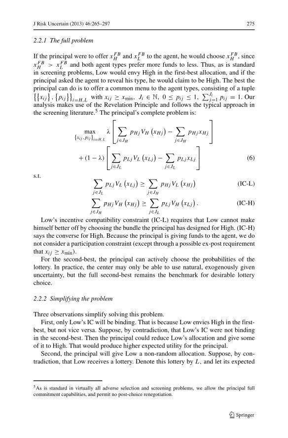
Funds

Benefits

Low type

High type

xLFB EH

*

VL(s*)

VL(b*)

s* z* b* xHFB

VL(z*)

Fig. 1 Second-best screening allocation (Notation given in text)

we also have that if Low is more risk-averse than High, he is also more downsiderisk-averse.8

Figure 1 plots the optimal allocations for the case of a lower bound of xmin = 0(a rescaling that provides an intuitive reference point without sacrificing generality).For simplicity, the figure assumes that the ratio of Low’s benefit to High’s benefitgoes to unity (and it draws the x-axis at that level), but this is obviously not required.

The solid line in Fig. 1, connecting the utility levels VL (b∗) and VL (s∗) , allowsus to track the expected utility for Low when he mimics High. By Jensen’s inequality,the center can give High a larger expected allocation than Low, that is, E∗

H = p∗b∗ +(1 − p∗) s∗ > z∗.

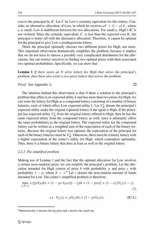
Figure 2 presents the solution in an alternative way. Expected utility maximizationmodels can be represented by a two-moment decision model under some conditions(Sinn 1983; Meyer 1987). Representing the principal’s problem in mean-variancespace has the advantage that we can see immediately the presence of a screeningcondition. In particular, in μ − σ− space (with volatility on the horizontal axis),indifference curves of more risk-averse agents are more steeply sloped. Under ourassumption that Low is more risk-averse, those with high productivity require feweradditional funds for any increase in fund variability than those with low productivity.Thus, the indifference curves look as in Fig. 2.

In the first-best, zero volatility is optimal, and High receives a larger allocationthan Low, as indicated by the points H −FB and L−FB, respectively. The second-

8We use a prudence-based definition of more downside risk-aversion. Liu and Meyer (2012) introducean alternative definition based on decreasing absolute risk aversion (DARA). The definitions are closelyconnected (see Section 4 in their paper).

280 J Risk Uncertain (2013) 46:265–297

Variance of allocation

High

Low

L-FB

H-FB

L-SB

H-SB

Expected allocation

Fig. 2 Representation of the second-best screening allocation in μ–σ space

best, compared to the first-best, employs a higher certain allocation for Low (and stillno volatility) and a lower expected and more risky allocation for High, as indicated bythe points H − SB and L − SB, respectively. The principal trades off giving a largerexpected amount to High against having to do this with greater risk in order to keepLow from mimicking High. The second-best solution optimally balances these twoobjectives, such that Low is just indifferent (as can be seen by the fact that L − SB

and H − SB lie on the same indifference curve for Low).

3 Discussion and interpretation

3.1 The correlation between marginal productivity and risk tolerance

The separation of High and Low depends on the positive correlation betweenmarginal productivity and risk tolerance. (When High is less risk-tolerant, the bestthat the principal can do is to offer a fixed budget, i.e., an identical allocation to thetwo types). How plausible is the positive correlation assumption?

For the production case, it is straightforward to think of situations in which oneagent (a division, for example) is more marginally productive and has a less curvedproduction function, effectively making the agent more risk tolerant than anotheragent. The same factors that lead marginal productivity to be larger for High plausiblyalso lead to marginal productivity declining more slowly. For example, consider man-agerial talent. A talented manager is not only better at making workers productive,but he is also better at maintaining those productivity gains for additional workers.

The consumption case is more subtle, but economic intuition suggests that thepositive correlation may be a good starting point. Suppose that two agents receive,in fact, the same marginal benefits from an incremental dollar. Then the one who ismore risk-tolerant — that is, who has a benefit function that flattens out more slowly

J Risk Uncertain (2013) 46:265–297 281

— will benefit more from a more-than-incremental windfall. To determine the pres-ence or absence of the correlation between being risk-tolerant and being a connoiseur,we conducted surveys among Masters and Ph.D. students in Public Policy at HarvardUniversity (the “Harvard sample”), two separate groups of undergraduate studentsof economics and psychology at the University of Zurich (“undergraduate sample 1”and “undergraduate sample 2”), and undergraduate students of finance at the Univer-sity of Zurich (the “finance sample”). In total, 339 subjects participated. We pool datafrom all samples. In the regression analysis we use dummies to identify each sample.

The questionnaire consisted of two parts. (See Appendix B for details). First, weemployed a widely used format of asking for the degree of risk tolerance, entailingpairwise comparisons of a risky choice and a certain outcome. In essence, the seriesof questions we asked culminated in an answer to the question: Consider a fair lotterywhere you have a 50% chance of doubling your income, and a 50% chance of losinga certain percentage, say x% of your income. What is the highest loss x that youwould be willing to incur to agree to taking part in this lottery? Similar questions areproposed by Gollier (2001); Mankiw and Zeldes (1991), and others.9 Our averagefinding of x% = 26% is consistent with the finding of Barsky et al. (1997) whoreport an average of x = 23%.

Second, we confronted participants with two (imaginary) situations. In situation 1,participants were asked to imagine that they had found a Swiss Franc 50 note (US$50in the Harvard sample), while in situation 2, participants were asked to imagine thatthey had just won in a lottery an amount of Swiss Franc 500,000 (US$500,000 in theHarvard sample). In both situations, we asked participants to compare themselves toa peer of similar wealth and income and answer whether they would derive muchgreater, greater, equal, less or much less welfare from these positive events. Whilethe average of participants answered that they would benefit about the same as theirpeers, there was substantial variation in the answers. Figure 3 plots the mean risktolerance levels in the various categories and the corresponding standard errors.

Figure 3 illustrates the central finding of this analysis: There is a strong posi-tive correlation between risk tolerance and a subjective feeling of being able to usewindfall funds in a more effective, utility-enhancing way than one’s peers.10

9A large literature deals with methods of eliciting risk preferences. Anderson and Mellor (2009) establishthat risk preference estimates can vary greatly across elicitation methods. We opted for a simple approachbecause we wanted to avoid a dependence of the results on the perhaps heterogeneous numerical skillsof survey participants in our overall sample (Dave et al. 2010). Results in Hey et al. (2009) suggest thatpairwise choice methods of the type underlying our survey tend to be less noisy than alternative methods.Of course, a drawback of our approach is that given the magnitude of stakes of interest, we had to askhypothetical questions.10We coded the answers into the five categories and created variables MU50 and MU500k, where MUdenotes marginal utility. Higher numbers denote higher stated marginal benefits. Because our marginalbenefits variables are ordinal, we used rank-order correlations to statistically determine its relationshipwith risk tolerance. Both the Spearman correlation coefficient and Kendall’s tau are positive and indicatea highly statistically significant relationship, with p-values of 0.05 for the US$/Swiss Franc 50 questionand below 0.01 for the US$/Swiss Franc 500,000 question. We also ran regressions with risk toleranceas the dependent variable and marginal benefits as the key explanatory variable (and sample dummies ascontrols), obtaining the same findings. The detailed results are available on request.

282 J Risk Uncertain (2013) 46:265–297

15

20

25

30

35

40

muchless

less same more muchmore

muchless

less same more muchmore

Mea

n r

isk

tole

ran

ceHow much do you benefit from an extra US$/Swiss Franc 50 (left panel) /

from an extra US$/Swiss Franc 500,000 (right panel) compared to your peers?

Fig. 3 Risk tolerance and stated marginal benefits. The panel on the left plots mean risk tolerance levelsand standard errors in the five marginal benefit categories for the US$ /Swiss Franc 50 question (N = 275).The panel on the right does the same for the US$ /Swiss Franc 500,000 question (N = 232). Total N = 339(some participants answered both questions). For details on the survey see the text and Appendix B

We interpret this as being consistent with the assumption that High marginal util-ity types (connoisseurs) are more risk-tolerant. Thus, the findings are supportiveof Solomon’s working hypothesis.11 Clearly, this approach is limited and merelyexploratory, because it relies on introspection and subjective assessments, employssolely student subjects, and does not involve actual monetary stakes.

Also, there may be unobserved heterogeneity in the population. For example,if survey participants differ substantially on wealth, then answers to our surveyquestion on marginal utility would miss this unobserved variable. In general, wewould expect poorer individuals to have higher marginal utility of wealth and tobe less risk-tolerant. (Evidence in Dohmen et al. (2010) suggests, for example, thatcredit-constrained individuals exhibit a lower willingness to take risks). Therefore,unobserved unequal wealth levels are likely to work against the empirical assump-tion of the model. Thus, our findings of a positive correlation despite the differential

11The data from Solomon’s surveys, alas, are lost in history. Our surveys thus add modestly to theknowledge about the joint distribution of risk attitudes and preference intensity in the population. Otherresearchers, while not yet familiar with Solomon’s Lost Scroll, have also found evidence that is consis-tent with his observation. In particular, Dohmen et al. (2010) present evidence that individuals with highercognitive abilities are less risk-averse. Donkers et al. (2001) find that, controlling for income, educationis positively associated with risk tolerance. Grinblatt et al. (2011) show that higher IQ individuals partic-ipate in the stock market to a greater exent. If the principal wishes to give more funds to an agent withhigher cognitive abilities (who may be able to use these funds more productively for his and the principal’sbenefit), this supports the effectiveness of Solomon’s screening method.

J Risk Uncertain (2013) 46:265–297 283

wealth factor suggest that the positive relationship holding wealth constant must bestrong. Moreover, in many practical circumstances, we believe, the principal willhave firm prior information about the wealth level of her agents, which she can takeinto account in her allocation decisions.

Differing decision-making abilities may produce a second realm of unobservedheterogeneity. This phenomenon will often work in favor of the assumption: Moreable agents find more value-generating uses of funds, and they may also avoid theexcessive risk aversion well documented for small gambles (Rabin 2000).

We recognize, of course, that principals may not merely be interested in allocatingresources where they offer the highest marginal utility, hence achieving the highesttotal utility. They may feel, for example, that less able agents should receive more,even if they will not put resources to the highest value use. If promoting total utilityis not the goal, then our analysis is silent.

3.2 When is separation not profitable?

Even when screening is possible, it does not always pay. To see the intuition, considerthe alternative to screening, namely allocating the optimal identical amount to bothtypes. The principal would solve:

maxy

λ [VH (y)] + (1 − λ) [VL(y)] − y, (8)

leading to a y∗ that satisfies:

λV ′H

(y∗) + (1 − λ)V ′

L

(y∗) = 1. (9)

Note that as the fraction of one of the two types increases, the fixed budget alloca-tion y∗ resembles more the first-best of that type and less the first-best of the othertype. In the limiting case, of course, lim λ−→1y

∗ = xFBH and limλ−→0y

∗ = xFBL .

There is, however, a crucial difference between the types: Fixed budgets alwaysgive too much to Low, and too little to High. In addition, this distortion is costlierfor High, and hence to the principal as well, because he has greater marginalbenefits.

Of course, no allocation can outperform the first-best. We also know that thesecond-best approximates the first-best arbitrarily closely under the conditions wefound above. Thus, the principal is always able to improve just a little bit on anyproposed solution in the second-best. As the fraction of High types (λ) increases,fixed budgets become more efficient. To retain the superiority of screening overfixed budgets, as λ increases, the principal makes the lottery ever more extreme,pushing s∗ further and further down towards xmin. Consequently, it always paysfor her to screen in this case. This result is stated in part (i) of the Propositionbelow.

When the principal is constrained in her ability to achieve the first-best, things turnout to be different and a fixed budget for both High and Low can become a seriouscompetitor to second-best screening. When the fraction of High types increases, theprincipal may be limited in her abilities to adjust the allocations. As shown, in the

284 J Risk Uncertain (2013) 46:265–297

typical case, she is already at the lower limit with the prize in the bad state. Then,the only way to avoid Low envying High is to increase the allocation to Low or theallocation to High in the good state (suitably adjusting the probabilities in High’slottery so that the associated risk is sufficiently unattractive for Low). It is, however,never optimal to increase High’s allocation beyond the first-best. Doing so would buythe principal a second-order gain at a first-order cost, because at that level of funds,the marginal cost is greater than the marginal benefit. Therefore, a single fixed budgetmay become optimal.

Conversely, as the fraction of Low types increases (λ decreases), the fixed budgetstrategy becomes less efficient, because, after all, High’s marginal productivity ishigher. Of course, with many Low and few High types, the screening solution alsobecomes less attractive. Appendix A shows that the first effect dominates the second.Intuitively, the loss in efficiency from screening comes from distorting High, butif the fraction of High types is small, it costs virtually nothing to distort them. Insum, if screening pays for some fraction of Low types, it also pays for all greaterfractions.

A final important determinant of the decision whether to screen is whether thetypes are sufficiently different, compared to the costs of funds. Intuitively: Even ifthe fraction of Lows is high, the center may do well enough with fixed budgets ifLows and Highs are not that different and if costs are sufficiently high, implying thateven in the first-best the principal would give them almost equal allocations. Theseinsights are summarized in the following:

Proposition 3 Consider a fixed budget as an alternative to screening.

(i) If limx→xmin V ′L(x)/V ′

H(x) = ∞, screening is always profitable.(ii) Suppose limx→xmin V ′

L(x)/V ′H(x) = C < ∞.

a) If Low is sufficiently risk-averse, then it pays to screen.b) If screening is profitable at some fraction of Low types, it remains

profitable at all greater fractions of Low types.

Proof See Appendix A.

3.3 Two time periods

While we have framed the screening problem as one of choosing the optimal pair ofa non-random budget and a random allocation, it is also useful to consider the case oftwo periods when no learning about productivity takes place between periods. Nowwe assume that a bundle the principal can offer consists of a certain allocation ineach of the periods, and that agents cannot shift resources between periods. Supposeutility is additive across periods.

Begin with the case where there are two time periods of equal length, and dis-counting is set aside for simplicity. Let xi be the first period allocation for type i,and let yi be the second period allocation for that type. In the first-best, xFB

H =yFBH > xFB

L = yFBL . As before, we know immediately that there is no point in

giving different allocations to Low (over time). Only High’s allocation needs to be

J Risk Uncertain (2013) 46:265–297 285

distorted in order to make it unattractive for Low. The principal’s problem in thiscase is:

max λ [VH (xH ) + VH (yH ) − (xH + yH )] + (1 − λ) [VL (xL) + VL (xL) − (xL + xL)] (10)

s.t. 2VL (xL) ≥ VL (xH ) + VL (yH ) (IC-L)

One solution that is consistent with Low’s IC would be xH = yH . But since notboth xH and yH can be greater than xL = yL, the only solution would be for allspending amounts to be equal, as in the fixed-budgets case. But it is easy to seethat this cannot be optimal for the principal. Thus, we can check the possibility thatxH > xL = yL > yH . (The case of xH < xL = yL < yH is symmetric). Doingsimilar calculations as before, we arrive at the following:

Proposition 4 The principal can separate high and low-productivity types by offer-ing one sufficiently variable package and one package with constant funds over time.In particular:

1. xFBH > x∗

H > x∗L = y∗

L > max{xFBL , y∗

H

}.

2. x∗H + y∗

H > x∗L + y∗

L.

Result 2 can also be written asx∗H +y∗

H

2 > x∗L, indicating that the expected

per-period allocation to High is bigger than the expected per-period allocationto Low.

Note that with this scheme the principal will not be able to achieve close tofirst-best target efficiency. In particular, this case operates as if the principal wererestricted to using lotteries with equal probability on both prizes. But if time becomesdivisible (preferably infinitely so), then the principal can shorten the time periodspent consuming the low prize (i.e., reduce the weight on yH ), and lengthen the timeperiod for the high prize. If the principal can choose both the time periods and theprizes, the problem becomes equivalent to the main case.

3.4 Multiple types

The analysis extends to the case where there are N agent types. Normalize types suchthat V ′

1(x) < V ′2(x) < ... < V ′

N(x) for all x. In the first-best, xN > xN−1 > ... > x1.

Characterizing the second-best in the case where marginal utility of the lowesttype goes to infinity faster than that of the other types as funds approach the lowerbound proceeds, in principle, along the same lines as the two-type analysis. Consider,for example, three types. Only the local upward incentive compatibility constraintswill bind. The lowest type receives a non-random prize. The principal needs tomake sure that he does not envy the Medium type. Thus, she gives the Mediumtype a lottery with a high probability on Medium’s first-best, and a low probabil-ity on a very low prize. Also, the center needs to assure that Medium does not envyHigh. Thus, High will receive a very high probability on his first-best and a lowprobability on an even worse prize than the bad prize for Medium. Note that the

286 J Risk Uncertain (2013) 46:265–297

proof of the equivalence of an N-prize lottery to a two-prize lottery applies hereas well.

Depending on the fractions of Lows and Mediums in the population, and depend-ing on how tight the bounds are on the low prizes for the productive types, theprincipal may do far better with screening, or may do no better than with identicalbudgets. When Low’s and Medium’s ratios of marginal benefits, respectively, to thenext higher type’s marginal benefits are bounded, screening may still be desirable.If so, the principal achieves welfare in between the first-best and the fixed budgetsallocation.

3.5 Numerical results

We can use numerical simulations to verify the analytical results and to quantify thewelfare gains. An Online Appendix shows the results of such simulations for CRRAand CARA benefit functions.

4 Conclusion and applications

In many important contexts, a principal allocates resources to agents who thenemploy those resources to create benefits for both themselves and the principal. Achallenge arises when, as is frequent, the principal does not know the agents’ abilitiesto create such benefits. Such problems arise in fairy tales, within the family, the cor-poration, and with nonprofit and government programs. In fairy tales, the benevolentking wishes to find out which of the suitors loves his daughter the most. Perhaps themost common everyday example is the parent distributing resources to a child, notknowing how much benefit the child will receive from them. In the business world, acorporate center allocates resources to divisions, not knowing what level of produc-tion or profitability will be reaped from those resources. In academia, deans allocateslots and funds to different departments, but are likely to be only partially informedon what benefits they will bring to the school. In the world of nonprofits, the philan-thropist provides funding to a variety of endeavors, but does not know how effectiveeach will be in promoting her causes. The common characteristic of all these casesis that the principal’s benefit is strongly related, and possibly directly proportional,to those of her agents. Thus, the agent is the source of the principal’s benefits. Nev-ertheless, a divergence of interests arises, because an agent is solely interested in hisown productivity, and rarely pays fully for his own budget. The principal is concernedwith the productivity of all agents.

Our central result is that a principal can successfully separate differentially pro-ductive types by using the insight that the degree to which an agent produces marginalbenefits from funds can be (and plausibly frequently is) positively correlated withthe source’s effective tolerance for risk. If this correlation between risk tolerance andproductivity holds, the optimal allocation of resources requires giving fixed funds tothe less productive type, but a surprisingly extreme lottery to the productive type. TheHigh producer demonstrates his capabilities by taking excess risk, such as accept-ing a very small but positive probability of receiving a small allocation of resources.

J Risk Uncertain (2013) 46:265–297 287

When benefits to Low fall without bound and faster than benefits to High as resourcesdecrease (as is the case for constant relative risk aversion benefit functions, which arefrequently used in economic modeling), the center is able to approximate first-bestexpected welfare very closely, even if negative payments are not permitted. Whennegative payments are allowed, e.g., if individuals have endowments that the princi-pal can cut, the principal can always get almost first-best welfare for herself and forthe source. Although the extreme lottery required for this outcome may be hard toimplement politically, it provides an important benchmark result for applications.

In practice, centers can use the external world as a randomization device, evenwithout necessarily aiming to optimize the probabilities associated with the prizes.Indeed, the model implies that a center may not wish to minimize uncertainty becauseof the opportunities it generates for effective screening. The extreme lottery result ofProposition 2 even suggests that in many circumstances it is beneficial to the centerto have at its disposal extreme downside risks that occur with very low probability.As such, the model helps understand some arrangements in the real world, and itoffers recommendations for an improved use of resources. For example, many indi-viduals pursuing job alternatives have the choice between a risky and a safe job.The model explains why a firm (say a university) might want to have its job risky:This property offers a mechanism for assuring that the person would benefit greatlyfrom the position. Thus, the candidate will not leave quickly for another position. Asanother example, family companies often encounter the paper’s separation problemand sometimes use versions of the proposed solution when implementing succes-sion plans, aiming to give the company to the most deserving heir.12 Finally, as anexample of the concrete normative implications of the model, a venture capital fund,in trying to screen out unproductive investments, may employ the method proposedhere. If it thinks there is a correlation between productivity and risk tolerance, saybecause entrepreneurs with a better idea will have a better fallback, then it could offerentrepreneurs a risky package. Thus, the venture capital investors would not insureentrepreneurs if some extreme untoward event happened, even though efficient riskspreading would recommend they should. Note that in principle this has nothing to dowith motivating effort, just assessing productivity. Of course, in real world contextseffort choice will play an additional role.

Thus, in a variety of settings, gauging the intensity of preferences based on risktaking can provide a powerful method to increase target efficiency. This screeningtool will be effective whenever there is a positive correlation between marginal ben-efits and tolerance for risk. We argued that this is a plausible condition when centralresources must be allocated to corporate divisions. Our empirical samples for the

12Consider the following real case. The founder and CEO of Spedag group, a leading Swiss logistics com-pany, had three children, A, B, and C. He wanted the child who felt he could get the most value to leadthe company. He did not want to separate ownership and control. (Skill may have been an additional con-sideration). He separated the original company into an operating company (OP), and a holding company(H). H initially owned everything. Son A received a personal loan from H enabling him to buy OP fromit. OP also rented buildings from H. Daughter B and son C received part of the price that A paid as anadvance on their inheritance, but were excluded from the business. Son A, as sole owner and CEO of OPbears substantial risk, but in expectation felt his holdings were worth significantly more than the advancespaid to B and C. B and C received enough that they were happy to accept this arrangement.

288 J Risk Uncertain (2013) 46:265–297

consumption case, drawn from Switzerland and the US, found our required conditionsatisfied: Risk tolerance and marginal benefits from resources were positively corre-lated. Given this straightforward condition, whether dealing with for-profit entitiesor individuals as beneficiaries, resource allocation can be implemented wisely, usingthe system of Solomon.

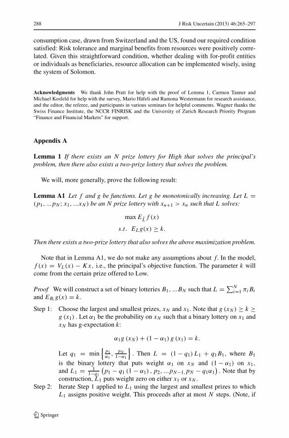
Acknowledgments We thank John Pratt for help with the proof of Lemma 1, Carmen Tanner andMichael Kosfeld for help with the survey, Mario Hafeli and Ramona Westermann for research assistance,and the editor, the referee, and participants in various seminars for helpful comments. Wagner thanks theSwiss Finance Institute, the NCCR FINRISK and the University of Zurich Research Priority Program“Finance and Financial Markets” for support.

Appendix A

Lemma 1 If there exists an N prize lottery for High that solves the principal’sproblem, then there also exists a two-prize lottery that solves the problem.

We will, more generally, prove the following result:

Lemma A1 Let f and g be functions. Let g be monotonically increasing. Let L =(p1, ...pN ; x1, ...xN) be an N prize lottery with xn+1 > xn such that L solves:

max ELf (x)

s.t. ELg(x) ≥ k.

Then there exists a two-prize lottery that also solves the above maximization problem.

Note that in Lemma A1, we do not make any assumptions about f. In the model,f (x) = VL(x) − Kx, i.e., the principal’s objective function. The parameter k willcome from the certain prize offered to Low.

Proof We will construct a set of binary lotteries B1, ...BN such that L = ∑Ni=1 πiBi

and EBi g(x) = k.

Step 1: Choose the largest and smallest prizes, xN and x1. Note that g (xN) ≥ k ≥g (x1) . Let α1 be the probability on xN such that a binary lottery on x1 andxN has g-expectation k:

α1g (xN) + (1 − α1) g (x1) = k.

Let q1 = min{

p1α1

,pN

1−α1

}. Then L = (1 − q1) L1 + q1B1, where B1

is the binary lottery that puts weight α1 on xN and (1 − α1) on x1,

and L1 = 11−q1

(p1 − q1 (1 − α1) , p2, ...pN−1,pN − q1α1

). Note that by

construction, L1 puts weight zero on either x1 or xN .

Step 2: Iterate Step 1 applied to L1 using the largest and smallest prizes to whichL1 assigns positive weight. This proceeds after at most N steps. (Note, if

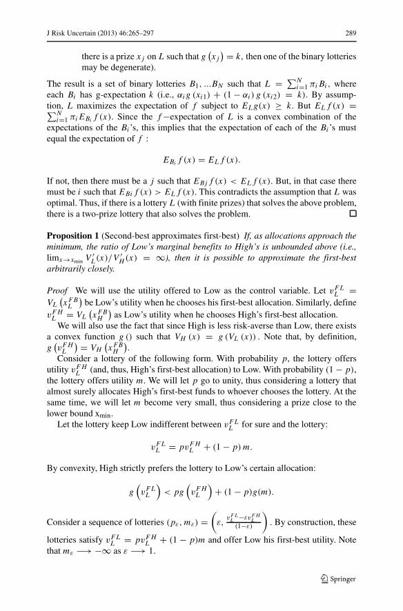
J Risk Uncertain (2013) 46:265–297 289

there is a prize xj on L such that g(xj

) = k, then one of the binary lotteriesmay be degenerate).

The result is a set of binary lotteries B1, ...BN such that L = ∑Ni=1 πiBi, where

each Bi has g-expectation k (i.e., αig (xi1) + (1 − αi) g (xi2) = k). By assump-tion, L maximizes the expectation of f subject to ELg(x) ≥ k. But ELf (x) =∑N

i=1 πiEBi f (x). Since the f −expectation of L is a convex combination of theexpectations of the Bi’s, this implies that the expectation of each of the Bi’s mustequal the expectation of f :

EBi f (x) = ELf (x).

If not, then there must be a j such that EBjf (x) < ELf (x). But, in that case theremust be i such that EBif (x) > ELf (x). This contradicts the assumption that L wasoptimal. Thus, if there is a lottery L (with finite prizes) that solves the above problem,there is a two-prize lottery that also solves the problem.

Proposition 1 (Second-best approximates first-best) If, as allocations approach theminimum, the ratio of Low’s marginal benefits to High’s is unbounded above (i.e.,limx→xmin V ′

L(x)/V ′H(x) = ∞), then it is possible to approximate the first-best

arbitrarily closely.

Proof We will use the utility offered to Low as the control variable. Let vFLL =

VL

(xFBL

)be Low’s utility when he chooses his first-best allocation. Similarly, define

vFHL = VL

(xFBH

)as Low’s utility when he chooses High’s first-best allocation.

We will also use the fact that since High is less risk-averse than Low, there existsa convex function g () such that VH (x) = g (VL (x)) . Note that, by definition,g

(vFHL

) = VH

(xFBH

).

Consider a lottery of the following form. With probability p, the lottery offersutility vFH

L (and, thus, High’s first-best allocation) to Low. With probability (1 − p),the lottery offers utility m. We will let p go to unity, thus considering a lottery thatalmost surely allocates High’s first-best funds to whoever chooses the lottery. At thesame time, we will let m become very small, thus considering a prize close to thelower bound xmin.

Let the lottery keep Low indifferent between vFLL for sure and the lottery:

vFLL = pvFH

L + (1 − p) m.

By convexity, High strictly prefers the lottery to Low’s certain allocation:

g(vFLL

)< pg

(vFHL

)+ (1 − p)g(m).

Consider a sequence of lotteries (pε, mε) =(

ε,vFLL −εvFH

L

(1−ε)

). By construction, these

lotteries satisfy vFLL = pvFH

L + (1 − p)m and offer Low his first-best utility. Notethat mε −→ −∞ as ε −→ 1.

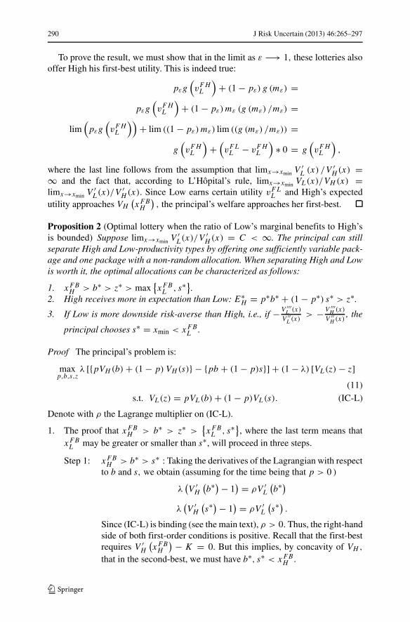
290 J Risk Uncertain (2013) 46:265–297

To prove the result, we must show that in the limit as ε −→ 1, these lotteries alsooffer High his first-best utility. This is indeed true:

pεg(vFHL

)+ (1 − pε) g (mε) =

pεg(vFHL

)+ (1 − pε)mε (g (mε) /mε) =

lim(pεg

(vFHL

))+ lim ((1 − pε) mε) lim ((g (mε) /mε)) =

g(vFHL

)+

(vFLL − vFH

L

)∗ 0 = g

(vFHL

),

where the last line follows from the assumption that limx→xmin V ′L (x) /V ′

H(x) =∞ and the fact that, according to L’Hopital’s rule, limx→xmin VL(x)/VH (x) =limx→xmin V ′

L(x)/V ′H(x). Since Low earns certain utility vFL

L and High’s expectedutility approaches VH

(xFBH

), the principal’s welfare approaches her first-best.

Proposition 2 (Optimal lottery when the ratio of Low’s marginal benefits to High’sis bounded) Suppose limx→xmin V ′

L(x)/V ′H (x) = C < ∞. The principal can still

separate High and Low-productivity types by offering one sufficiently variable pack-age and one package with a non-random allocation. When separating High and Lowis worth it, the optimal allocations can be characterized as follows:

1. xFBH > b∗ > z∗ > max

{xFBL , s∗}.

2. High receives more in expectation than Low: E∗H = p∗b∗ + (1 − p∗) s∗ > z∗.

3. If Low is more downside risk-averse than High, i.e., if −V ′′′L (x)

V ′′L(x)

> −V ′′′H (x)

V ′′H (x)

, the

principal chooses s∗ = xmin < xFBL .

Proof The principal’s problem is:

maxp,b,s,z

λ [{pVH (b) + (1 − p) VH(s)} − {pb + (1 − p)s}] + (1 − λ) [VL(z) − z]

(11)s.t. VL(z) = pVL(b) + (1 − p)VL(s). (IC-L)

Denote with ρ the Lagrange multiplier on (IC-L).

1. The proof that xFBH > b∗ > z∗ >

{xFBL , s∗}, where the last term means that

xFBL may be greater or smaller than s∗, will proceed in three steps.

Step 1: xFBH > b∗ > s∗ : Taking the derivatives of the Lagrangian with respect

to b and s, we obtain (assuming for the time being that p > 0 )

λ(V ′

H

(b∗) − 1

) = ρV ′L

(b∗)

λ(V ′

H

(s∗) − 1

) = ρV ′L

(s∗) .

Since (IC-L) is binding (see the main text), ρ > 0. Thus, the right-handside of both first-order conditions is positive. Recall that the first-bestrequires V ′

H

(xFBH

) − K = 0. But this implies, by concavity of VH ,

that in the second-best, we must have b∗, s∗ < xFBH .

J Risk Uncertain (2013) 46:265–297 291

Now, if we had b∗ = s∗, (IC-L) would collapse into VL (z∗) =VL (b∗), and, thus, z∗ = b∗. Thus, the principal would implement fixedbudgets, a contradiction to the Proposition’s premise. For the conditionfor screening to be worth it, see Corollary 1.

If screening pays, we must have b∗ = s∗, which implies p∗ = 0and p∗ = 1 (justifying the assumption we made at the beginning ofthis step).

Step 2: z∗ > xFBL : See the text for the argument that the center will not

introduce any risk into Low’s allocation. Taking the derivative of theLagrangian with respect to xL, we obtain

(1 − λ)(V ′

L

(z∗) − 1

) = −ρV ′L

(z∗) .

Since ρ > 0, the right-hand side is negative, and since V ′L

(xFBL

)−1 =0, we have, by concavity of VL, z∗ > xFB

L .Step 3: b∗ > z∗ > s∗ : Clearly this must be the case, because otherwise High

(Low) would receive more than Low (High) for sure and the accordingIC would be violated.

2. From (IC-L), we have VL (z∗) = EVL (b∗). Jensen’s inequality impliesEVL (b∗) < VL

(E∗

H

). Thus, z∗ < E∗

H .

3. Assume now that we also have −V ′′′L (x)

V ′′L(x)

> −V ′′′H (x)

V ′′H (x)

. The proof that s∗ = xmin

will proceed in 6 steps. (Per our assumptions, xFBL >xmin, which proves the

inequality).

Step 1: Consider lottery L = (b, p; s, 1 − p), a candidate optimum with s >

xmin. Consider an alternate lottery L′ = (y, q; x, 1 − q), where b >

y > s > x and q > p such that pb + (1 − p) s = qy + (1 − q)x andpUH (b) + (1 − p) UH (s) = qUH(y) + (1 − q)UL(x). That is, L andL′ have the same expected value and same expected utility for High. Itis easy to show that such L and L′ exists.

Step 2: According to Chiu (2010), Bernoulli lotteries are always (generalized)skewness comparable. Moreover, distribution F is more skewed to theright than distribution G if and only if F puts greater probability onthe small prize than G does. Hence, L is more skewed to the right thanL′. Another way to say this is that L′ has more downside risk than L.

Step 3: Theorem 2a in Chiu (2010) establishes that preferences over skew-ness comparable lotteries can be represented by a utility functionthat depends only on the mean (μ), variance

(σ 2

)and centralized

third moment(m3

)of the distribution. That is, there exists a function

U(μ, σ 2, m3

)that represents preferences, where U

(μ, σ 2, m3

) =∫u(x)dF (x). Furthermore, U

(μ, σ 2, m3

)is increasing in μ and m3

and decreasing in σ 2 if and only if u′ > 0, u′′ < 0, and u′′′ > 0.Step 4: Since High is indifferent between L and L′, and m3

L > m3L′ , it must be

that σ 2L > σ 2

L′ . Otherwise, L would have less risk and less downsiderisk, and High would necessarily prefer L to L′.

292 J Risk Uncertain (2013) 46:265–297

Step 5: Corollary 2 (Chiu 2005): Suppose u′′ < 0, v′′ < 0, and u′′′ > 0, andF and G are strongly skewness comparable, μF = μG, σF > σG, andmF > mG. If −v′′′(x)

v′′(x)≥ −u′′′(x)

u′′(x)and

∫u(y)dG(y) = ∫

u(y)dF (y),

then∫

v(y)dG(y) ≤ ∫v(y)dF (y).

Applying this in our context, it says that the assumption that Low

is more downside risk-averse than High, −V ′′′L (x)

V ′′L(x)

> −V ′′′H (x)

V ′′H (x)

, implies

that Low prefers L to L′.Step 6: Whenever s > xmin it is possible to construct lottery L′ that keeps High

as well off and has the same expected value as L. Since Low prefersL to L′, it is incentive compatible for the Principal to offer L′ to Highand amount z′ to Low, where z′ < z. Since z is greater than Low’s firstbest, the principal does better offering L′ and z′ than offering L and z.Hence L cannot be optimal.

Proposition 3 (Profitability of screening) Consider a fixed budget as an alternativeto screening.

(i) If limx→xmin V ′L(x)/V ′

H(x) = ∞, screening is always profitable.(ii) Suppose limx→xmin V ′

L (x) /V ′H (x) = C < ∞. (a) If Low is sufficiently risk-

averse, then it pays to screen. (b) If screening is profitable at some fraction ofLow types, it remains profitable at all greater fractions of Low types.

Proof Part (i) is trivial: Since we know under the stated condition, the second-bestapproximates the first-best arbitrarily closely, the principal can always find a way todo better than with a fixed budget.Part (ii)(a): The principal’s problem is:

maxp,b,s,z

λ [{pVH (b) + (1 − p) VH(s)} − {pb + (1 − p)s}]

+ (1 − λ) [VL(z) − z] (12)

s.t.

VL(z) = VL(ce (b, s, p)) . (IC-L)

where ce (b, s, p) = pVL(b) + (1 − p)VL(s), i.e., Low’s certainty equivalent forthe lottery (b, p; s, (1 − p)) . Consider the lottery with b = xFB

H , s = xmin andz = xFB

L . Three features of this lottery are worth noting. First, this lottery gives theprincipal less than the second-best welfare (because it deviates from the lottery weshowed to be optimal in Proposition 3). Second, note that as Low becomes infinitelyrisk-averse, ce (b, xmin, p) goes to zero. Hence, for Low sufficiently risk-averse, forany p there is a level of risk aversion of Low such that this lottery satisfies incentivecompatibility. Third, assume that the proposed lottery is incentive-compatible. Then,as p −→ 1, the optimal value of the principal’s objective function approaches thefirst-best.

J Risk Uncertain (2013) 46:265–297 293

Construct the following sequence:(

1n, V n

L

)where 1

nis the probability of the xmin

prize, and V nL is a utility function for Low with the following properties:

dV nL

(xFBL

)

dx= 1

and V n+1L is more risk-averse than V n

L , and:

V nL

(ce

(b, xmin, 1 − 1

n

))≤ VL

(xFBL

).

Thus, 1n

represents a sequence of probabilities going to zero, and V nL represents a

sequence of increasingly risk-averse utility functions for Low chosen so that Lowprefers his first-best amount for sure to the lottery intended for High.

By construction, this sequence is incentive compatible, and the value of the objec-tive function converges to the first-best as n −→ ∞. Finally, since no allocationmechanism can do better than the first-best, and since this lottery performs worsethan the actual second-best lottery characterized in Proposition 3, we know that ifLow is sufficiently risk-averse, it pays to screen.Part (ii)(b): Call the optimized value of the principal’s objective function in the aboveproblem OF(λ). Note that OF (λ) is continuous by, for example, Berge’s theorem.It is optimal to screen when there exist p, b, s, and z such that OF(λ) is greater thanthe optimal non-screening contract.

The optimal non-screening contract maximizes λVH(y) + (1 − λ) VL(y) − y. Lety (λ) denote the y (a single fixed budget) that solves this problem for a particu-lar λ, and let V NS (λ) denote the principal’s maximal utility in the no-screeningproblem. Note that y(0) = xFB

L , y(1) = xFBH , and y (λ) is increasing in λ. Since

VH (y) > VL(y), and increasing λ puts more weight on VH and increases the opti-mal y, V NS(λ) = λVH (y (λ)) + (1 − λ) VL (y (λ)) − y(λ) is increasing in λ. Inother words, V NS(λ) represents the “bar” for when it is optimal to screen, and thisbar decreases as λ decreases, i.e., the greater the fraction of Lows. The more Lowsthere are, the easier it is for screening to be optimal, for a given welfare derivedfrom screening. It is true that the welfare for the principal in the screening casealso decreases when λ decreases. But the first effect dominates the second. To seethis, suppose it is optimal to screen when λ = λ. This means that the value of

the constrained is such that OF(λ)

> V NS(λ)

. Since OF(λ)

is continuous,

OF(λ) > V NS(λ)

for λ close to λ. For λ < λ, V NS(λ) < V NS(λ)

. Hence for

λ < λ we have OF(λ) > V NS(λ)

> V NS(λ). This completes the proof.

Appendix B

As explained in the paper, we conducted surveys among Masters and Ph.D. stu-dents in Public Policy at Harvard University (the “Harvard sample”), two separate

294 J Risk Uncertain (2013) 46:265–297

groups of undergraduate students of economics and psychology at the Univer-sity of Zurich (“undergraduate sample 1” and “undergraduate sample 2”), andundergraduate students of finance at the University of Zurich (the “finance sam-ple”). The undergraduate sample 1 and 2 participants were paid a fee of SwissFranc 15 for filling out the questionnaire. In addition to filling out the sur-vey, the undergraduate sample students had an opportunity to earn another SwissFranc 15 in a non-related cognitive task designed for another project. The orderof tasks was randomized and there was no statistically significant difference inanswers depending on the order. The other subjects only filled out the question-naire. The finance sample was collected through an online survey; the otherswere collected by paper surveys. In the finance sample, 63% of the studentsanswered only the question in situation 1, while 37% of the students only answeredsituation 2.

For the analysis shown in the paper, we only use the questionnaires from indi-viduals who answered the risk aversion questions consistently (which was the vastmajority of individuals). Thus, we did not use data of indivudals who accepted alottery where x = 30%, but rejected one where x = 10%. We also did not usedata of individuals who claimed their x was 23% but still accepted a lottery withx = 50%. Including the data of these (very few) individuals does not materiallyaffect the results.

In the survey, the currency of the respective country was used. In the US surveys,this was the US$. In the Swiss surveys, this was the Swiss Franc.

1. Please think about your total yearly income. Please put a checkmark next to thefollowing elements which form part of your definition of income.

a) Salary and other labor income, such as bonusesb) Interests, dividends, rental income, etc.c) Financial support from family membersd) Stipendse) Other, please list here

2. Please consider your total yearly income after taxes. There is no “correct” def-inition; please keep as comprehensive a definition of “income” in mind aspossible.

Let us suppose that you have the chance to double this income with a 50%probability. But to obtain this chance, you also have to accept the possibil-ity that your income decreases by x% with 50% probability. That is, we areflipping a coin. Assume, for example, that your income is $US/Swiss Franc30,000 and x = 20%. Then, after the coin is flipped, you either have an incomeof $US/Swiss Franc 60,000 or your income is reduced to $US/Swiss Franc24,000. Both events are equally likely, since heads and tails occur with equalprobability.

Are you willing to accept this opportunity and this risk, if

a) x = 10%, i.e., your income doubles with 50% probability and decreases by10% with 50% probabilityYES – NO

J Risk Uncertain (2013) 46:265–297 295

b) x = 90%, i.e., your income doubles with 50% probability and decreases by90% with 50% probabilityYES – NO

c) x = 20%, i.e., your income doubles with 50% probability and decreases by20% with 50% probabilityYES – NO

d) x = 50%, i.e., your income doubles with 50% probability and decreases by50% with 50% probabilityYES – NO

e) x = 30%, i.e., your income doubles with 50% probability and decreases by30% with 50% probabilityYES – NO

f) x = 40%, i.e., your income doubles with 50% probability and decreases by40% with 50% probabilityYES – NO

3. Assume now that you can choose the maximum loss level that you are willing toaccept, i.e., you can choose x between 0% and 100%. In other words, you willdouble your income, or lose x% of it, both with the same probability. How highwould you set x% and still accept playing this “lottery”?x = %

4. Please imagine that you find a $US/Swiss Franc 50 note on the street. It isimpossible to identify the owner, and it is, therefore, completely acceptable andmorally unobjectionable that you keep the $US/Swiss Franc 50. Think aboutyour average peer who earns about the same amount of money as you do, and isapproximately equally wealthy. Would you say that, relative to this average peer,you benefit

• a lot more• more• equally• less• a lot less

from this additional amount of money?

5. Please imagine now that a very distant relative, whom you have never heardof, dies and happens to leave you $US/Swiss Franc 500,000. Think about youraverage peer who earns about the same amount of money as you do, and isapproximately equally wealthy. Would you say that, relative to this average peer,you benefit

• a lot more• more• equally• less• a lot less

from this additional amount of money?

296 J Risk Uncertain (2013) 46:265–297

References

Akerlof, G. (1970). The market for ‘lemons,’ qualitative uncertainty and the market mechanism. QuarterlyJournal of Economics, 84(3), 488–500.

Anderson, L.R., & Mellor, J.M. (2009). Are risk preferences stable? Comparing an experimental measurewith a validated survey-based measure. Journal of Risk and Uncertainty, 39(2), 137–160.

Antle, R., & Eppen, G.D. (1985). Capital rationing and organizational slack in capital budgeting.Management Science, 31(2), 163–174.

Arnott, R., & Stiglitz, J.E. (1988). Randomization with asymmetric information. RAND Journal ofEconomics, 19(3), 344–362.

Barsky, R.B., Juster, T.F., Kimball, M.S., Shapiro, M.D. (1997). Preference parameters and individualheterogeneity: an experimental approach in the health and retirement study. Quarterly Journal ofEconomics, 112(2), 537–579.

Bernardo, A.E., Cai, H., Luo, J. (2001). Capital budgeting and compensation with asymmetric informationand moral hazard. Journal of Financial Economics, 61(3), 311–344.

Bernardo, A.E., Cai, H., Luo, J. (2004). Capital budgeting in multidivision firms: information, agency, andincentives. Review of Financial Studies, 17(3), 739–767.

Brams, S.J. (2005). Fair division. In B.R. Weingast, & D. Wittman (Eds.), Oxford handbook of politicaleconomy. Oxford: Oxford University Press.

Brams, S.J., & Kilgour, D.M. (2001). Competitive fair division. Journal of Political Economy, 109(2),418–443.

Brams, S.J., & Taylor, A.D. (1999). The win-win solution: guaranteeing fair shares to everybody. NewYork: W.W. Norton.

Brito, D.L., Hamilton, J.H., Slutzky, S.M., Stiglitz, J.E. (1995). Randomization in optimal income taxschedules. Journal of Public Economics, 56(2), 189–223.

Chiu, W.H. (2005). Skewness preference, risk aversion, and the precedence relations on stochastic changes.Management Science, 51(12), 1816–1828.

Chiu, W.H. (2010). Skewness preference, risk taking and expected utility maximization. Geneva Risk andInsurance Review, 35(2), 108–129.

Dave, C., Eckel, C.C., Johnson, C.A., Rojas, C. (2010). Eliciting risk preferences: when is simple better?Journal of Risk and Uncertainty, 41(3), 219–243.

Dohmen, T., Falk, A., Huffman, D., Sunde, U. (2010). Are risk aversion and impatience related to cognitiveability? American Economic Review, 100(3), 1238–1260.

Donkers, B., Melenberg, B., van Soest, A. (2001). Estimating risk attitudes using lotteries: a large sampleapproach. Journal of Risk and Uncertainty, 22(2), 165–195.

Golec, J., & Tamarkin, M. (1998). Bettors love skewness, not risk, at the horse track. Journal of PoliticalEconomy, 106(1), 205–225.

Gollier, C. (2001). The economics of risk and time. Cambridge: The MIT Press.Grinblatt, M., Keloharju, M., Linnainmaa, J. (2011). IQ and stock market participation. Journal of Finance,

66(6), 2124–2164.Harris, M., & Raviv, A. (1996). The capital budgeting process: incentives and information. Journal of

Finance, 52(1), 111–133.Harris, M., & Townsend, R.M. (1981). Resource allocation under asymmetric information. Econometrica,

49(1), 33–64.Harris, M., Kriebel, C.H., Raviv, A. (1982). Asymmetric information, incentives and intrafirm resource

allocation. Management Science, 28(6), 604–620.Hellwig, M.F. (2007). The undesirability of randomized income taxation under decreasing risk aversion.

Journal of Public Economics, 91(3–4), 791–816.Hey, J.D., Morone, A., Schmidt, U. (2009). Noise and bias in eliciting preferences. Journal of Risk and

Uncertainty, 39(3), 213–235.Leland, H.E., & Pyle, D.H. (1977). Informational asymmetries, financial structure, and financial interme-

diation. Journal of Finance, 32(2), 371–387.Liu, L., & Meyer, J. (2012). Decreasing absolute risk aversion, prudence and increased downside risk

aversion. Journal of Risk and Uncertainty, 44(3), 243–260.Mankiw, N.G., & Zeldes, S.P. (1991). The consumption of stock holders and non stock holders. Journal

of Financial Economics, 29(1), 97–112.

J Risk Uncertain (2013) 46:265–297 297

Maskin, E., & Riley, J. (1989). Optimal multiunit auctions. In F. Hahn (Ed.), The economics of missingmarkets and information. Oxford: Oxford University Press.

Meyer, J. (1987). Two-moment decision models and expected utility maximization. American EconomicReview, 77(3), 421–430.

Miller, N., Piankov, N.E., Zeckhauser, R.J. (2006). Possibly-final offers. Journal of Economics andManagement Strategy, 15(3), 789–819.

Moselle, B., Degeorge, F., Zeckhauser, R.J. (2005). Conspicuous conservatism in risk choice. Journal ofRisk and Uncertainty, 35(1), 1–16.

Pratt, J.W. (2005). Fair (and not so fair) division. Journal of Risk and Uncertainty, 35(3), 203–236.Pratt, J.W., & Zeckhauser, R.J. (1990). The fair and efficient division of the Winsor family silver.

Management Science, 36(11), 1293–1301.Rabin, M. (2000). Risk aversion and expected-utility theory: a calibration theorem. Econometrica, 68(5),

1281–1292.Salanie, B. (2005). The economics of contracts: a primer, 2nd edn. Cambridge: MIT Press.Sinn, H.-W. (1983). Economic decisions under uncertainty. Amsterdam et al.: North-Holland.Stein, J.C. (1997). Internal capital markets and the competition for corporate resources. Journal of Finance,

52(1), 111–133.Steinhaus, H. (1948). The problem of fair division. Econometrica, 16(1), 101–104.Stiglitz, J.E. (1982). Self-selection and Pareto efficient taxation. Journal of Public Economics, 17(2), 213–

240.Wakker, P.P., Thaler, R.H., Tversky, A. (1997). Probabilistic insurance. Journal of Risk and Uncertainty,

15(1), 7–28.Weiss, L.W. (1976). The desirability of cheating incentives and randomness in the optimal income tax.

Journal of Political Economy, 89(6), 1343–1352.