Solitons and periodic solutions to a couple of fractional nonlinear evolution equations

$Page 1: Solitons and periodic solutions to a couple of fractional nonlinear evolution equations$
PRAMANA c© Indian Academy of Sciences Vol. xx, No. x— journal of Month 2014

physics pp. 1–12

Solitons and periodic solutions to a couple of fractionalnonlinear evolution equations

M MIRZAZADEH1,∗, M ESLAMI2 and ANJAN BISWAS3,4

1Department of Engineering Sciences, Faculty of Technology and Engineering, East of Guilan,University of Guilan, Rudsar, Iran2Department of Mathematics, Faculty of Mathematical Sciences, University of Mazandaran,Babolsar, Iran3Department of Mathematical Sciences, Delaware State University, Dover, DE 19901-2277, USA4Faculty of Science, Department of Mathematics, King Abdulaziz University, Jeddah 21589,Saudi Arabia∗Corresponding author. E-mail: [email protected]

DOI: 10.1007/s12043-013-0679-0

Abstract. This paper studies a couple of fractional nonlinear evolution equations using first inte-gral method. These evolution equations are foam drainage equation and Klein–Gordon equation(KGE), the latter of which is considered in (2 + 1) dimensions. For the fractional evolution, theJumarie’s modified Riemann–Liouville derivative is considered. Exact solutions to these equationsare obtained.

Keywords. First integral method; solitons; foam drainage equation; Klein–Gordon equation.

PACS Nos 02.30.Jr; 05.45.Yv

1. Introduction

The theory of nonlinear evolution equations (NLEEs) has applications in several areas ofapplied mathematics, theoretical physics and engineering sciences [1–40]. Therefore,it is imperative to carry out a deeper investigation of these equations. So far, theseNLEEs were studied with integral-order temporal derivative or integer-order evolution.It is about time to generalize these evolution terms to fractional order so that this willlead to fractional-order evolution equations. The advantage of fractional derivatives, overinteger derivatives, is that it is related to the memory and heredity of several materials andprocesses. In addition, temporal fractional evolution is more realistic to describe manyphysical phenomena [39].

This leads to a more generalized setting so that the results of NLEEs with integer ordercan be considered as a special case. This paper addresses a couple of NLEEs that appear

Pramana – J. Phys., Vol. xx, No. x, Month 2014 1

M Mirzazadeh, M Eslami and Anjan Biswas

in engineering science and theoretical physics with fractional evolution. They are foamdrainage equation and Klein–Gordon equation, the latter of which is considered in (2+1)dimensions.

Foam drainage is the flow of liquid through foam when the effects of capillarity andgravity are taken into consideration. The physics of foam drainage and the issue ofcreaming in emulsions lead to this equation. This study was inspired by forced drainageexperiments where foam was injected from the top with liquid supply. Subsequently,the temporal and spatial variations of the liquid supply is determined [40]. This is animportant area of research in the detergent industry.

Klein–Gordon equation (KGE), on the other hand, is a relativistic field equationfor scalar particles (spin-0). KGE is a relativistic generalization of the well-knownSchrödinger’s equation. While there are other relativistic wave equations, KGE has beenthe most frequently studied equation for describing particle dynamics in quantum fieldtheory [4].

Jumarie [19] presented a modification of the Riemann–Liouville definition whichappears to provide a framework for fractional calculus. In this paper, the fractional evo-lution terms for the evolution equations will be from Jumarie’s point of view. Also, themethodology of extracting solutions for these couple of NLEEs will be the first integralapproach. The main idea of this algorithm is to implement division theorem for twovariables in the complex domain based on the ring theory of commutative algebra.

The paper is arranged as follows. In §2, we describe briefly the modified Riemann–Liouville derivative. Section 3 gives the algorithmic approach to the first integral method.In §4 and 5, we apply this method to the nonlinear fractional foam drainage equation andthe generalized forms of time-fractional Klein-Gordon equation.

2. Jumarie’s modified Riemann–Liouville derivative

The Jumarie’s modified Riemann–Liouville derivative of order α is defined as [21]

Dαt f (t) = 1

�(−α)

∫ t

0(t − ξ)−α−1(f (ξ) − f (0))dξ, (1)

for α < 0,

Dαt f (t) = 1

�(1 − α)

d

dt

∫ t

0(t − ξ)−α(f (ξ) − f (0))dξ, (2)

for 0 < α < 1,

Dαt f (t) = (f (n)(t))(α−n), (3)

if n ≤ α ≤ n + 1, n ≥ 1.

We list some important properties for the modified Riemann–Liouville derivative asfollows:

Dαt tr = �(1 + r)

�(1 + r − α)tr−α, r > 0, (4)

Dαt (f (t)g(t)) = g(t)Dα

t f (t) + f (t)Dαt g(t), (5)

Dαt f (g(t)) = f ′

g(g(t))Dαt g(t) = Dα

g f (g(t))(g′(t))α. (6)

2 Pramana – J. Phys., Vol. xx, No. x, Month 2014

Fractional nonlinear evolution equations

3. First integral method

A fractional partial differential equation, say in two or three independent variablesx, y, t, is given by

P

(u,

∂u

∂t,

∂u

∂x,

∂u

∂y,

∂αu

∂tα,

∂αu

∂xα,

∂αu

∂yα,

∂2αu

∂t2α, ...

)= 0, (7)

where u = u(x, y, t) is an unknown function, P is a polynomial in u = u(x, y, t) and itsvarious partial derivatives, in which the highest order derivative and nonlinear term areinvolved.

The main steps of the first integral method [21] are summarized as follows:

Step I: Suppose

u(x, y, t) = U(ξ), ξ = k

�(1 + α)xα + l

�(1 + α)yα − λ

�(1 + α)tα, (8)

and then eq. (7) can be turned into the following nonlinear ordinary differentialequation (ODE):

Q

(U(ξ),

dU(ξ)

dξ,

d2U(ξ)

dξ 2, ...

)= 0, (9)

where U(ξ) is an unknown function, Q is a polynomial in the variable U(ξ) andits derivatives. If all terms contain derivatives, then eq. (9) is integrated whereintegration constants are considered zero.

Step II: We assume that eq. (9) has a solution in the form

U(ξ) = X(ξ), (10)

and introduce a new independent variable

Y (ξ) = dX(ξ)

dξ,

which leads to a new system of

dX(ξ)

dξ= Y (ξ),

dY (ξ)

dξ= G(X(ξ), Y (ξ)). (11)

Step III: By using the Division Theorem for two variables in the complex domain Cwhich is based on the Hilbert–Nullstellensatz Theorem [30], we can obtain onefirst integral to eq. (11) which can reduce eq. (9) to a first-order integrableordinary differential equation. An exact solution to eq. (7) is then obtained bysolving this equation directly.

Division Theorem: Suppose P(w, z) and Q(w, z) are polynomials in C[w, z], andP(w, z) is irreducible in C[w, ν]. If Q(w, z) vanishes at all zero points of P(w, z), thenthere exists a polynomial G(w, z) in C[w, z] such that

Q(w, z) = P(w, z)G(w, z).



4. Foam drainage equation

In this section, we shall apply the first integral method to obtain exact solutions of thenonlinear foam drainage equation with time and space-fractional derivatives [31]

Dαt u = u

2Dα

x Dαx u − 2u2Dα

x u + (Dαx u)2, 0 < α ≤ 1. (12)

The foam drainage equation is a model of the flow of liquid through channels and nodes(intersection of four channels) between the bubbles, driven by gravity and capillarity [32].

As in [21], we make transformation

u(x, t) = U(ξ), ξ = lxα

�(1 + α)− λtα

�(1 + α)(13)

and generate the reduced nonlinear ODE in the form

l2

2UU ′′ + λU ′ + l2(U ′)2 − 2lU 2U ′ = 0, (14)

where the prime denotes the differential with respect to ξ.

Using (10) and (11), eq. (14) is equivalent to the two-dimensional autonomous system

dX

dξ= Y,

dY

dξ= 4

lXY − 2λ

l2

Y

X− 2

Y 2

X. (15)

Now, we make the transformation

dη = dξ

X(16)

in eq. (15) to avoid the singular line X = 0 temporarily. Thus, system (15) becomes

dX

dη= XY,

dY

dη= 4

lX2Y − 2λ

l2Y − 2Y 2. (17)

Now, we are applying the Division Theorem to seek the first integral to system (17).Suppose that X = X(η), Y = Y (η) are the nontrivial solutions to (17), and Q(X, Y ) =∑N

i=0 ai(X)Y i is an irreducible polynomial in the complex domain C such that

Q(X(η), Y (η)) =N∑

i=0

ai(X(η))Y i(η) = 0, (18)

where ai(X), i = 0, 1, ..., N are polynomials of X and aN(X) �= 0. Equation (18) iscalled the first integral to system (17). Note that dQ/dη is a polynomial in X and Y, and



q [X(η), Y (η)] = 0 implies dQ/dη|(17) = 0. According to the Division Theorem, thereexists a polynomial g(X) + h(X)Y in the complex domain C such that

dQ

dη= dQ

dX.dX

dη+ dQ

dY.dY

dη

= (g(X) + h(X)Y )

N∑i=0

ai(X)Y i. (19)

In this example, we assume that N = 1 in eq. (18). Then, by equating the coefficients ofY i, i = 2, 1, 0, on both sides of (19), we have

Xa′1(X) = h(X)a1(X) + 2a1(X), (20)

Xa′0(X) =

(g(X) − 4

lX2 + 2λ

l2

)a1(X) + h(X)a0(X), (21)

g(X)a0(X) = 0. (22)

As a1(X) and h(X) are polynomials, from eq. (20), we deduce that h(X) = −2 anda1(X) must be a constant. For simplicity, we can take a1(X) = 1. Balancing the degreesof g(X) and a0(X), we conclude that deg(g(X)) = 0 and deg(a0(X)) = 2 only.

Suppose

g(X) = A0,

a0(X) = B0 + B1X + B2X2, B2 �= 0, (23)

where A0, B0, B1, B2 are all constants to be determined.Substituting a0(X), a1(X) and g(X) into (21) and (22) and setting all the coefficients of

powers X to be zero, we obtain a system of nonlinear algebraic equations and by solvingit we get the solution set

A0 = 0, B0 = λ

l2, B1 = 0, B2 = −1

l, (24)

where l and λ are arbitrary constants.Using the conditions (24) in (18), we obtain

Y = λ

l2+ 1

lX2. (25)

Combining eq. (25) with eq. (17) and changing to the original variables, we find exactsolutions to eq. (12) as:

Case I. λl < 0:

u1(x, t) = −√−λ

ltanh

[√− λ

l3

(lxα

�(1 + α)− λtα

�(1 + α)+ ξ0

)](26)



and

u2(x, t) = −√−λ

lcoth

[√− λ

l3

(lxα

�(1 + α)− λtα

�(1 + α)+ ξ0

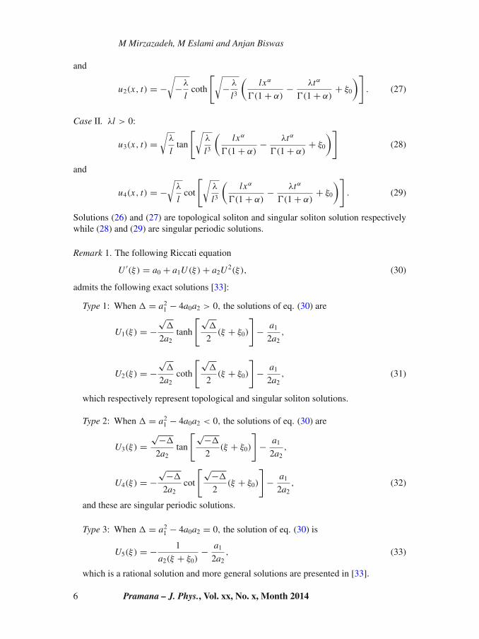
)]. (27)

Case II. λl > 0:

u3(x, t) =√

λ

ltan

[√λ

l3

(lxα

�(1 + α)− λtα

�(1 + α)+ ξ0

)](28)

and

u4(x, t) = −√

λ

lcot

[√λ

l3

(lxα

�(1 + α)− λtα

�(1 + α)+ ξ0

)]. (29)

Solutions (26) and (27) are topological soliton and singular soliton solution respectivelywhile (28) and (29) are singular periodic solutions.

Remark 1. The following Riccati equation

U ′(ξ) = a0 + a1U(ξ) + a2U2(ξ), (30)

admits the following exact solutions [33]:

Type 1: When = a21 − 4a0a2 > 0, the solutions of eq. (30) are

U1(ξ) = −√

2a2tanh

[√

2(ξ + ξ0)

]− a1

2a2,

U2(ξ) = −√

2a2coth

[√

2(ξ + ξ0)

]− a1

2a2, (31)

which respectively represent topological and singular soliton solutions.

Type 2: When = a21 − 4a0a2 < 0, the solutions of eq. (30) are

U3(ξ) =√−

2a2tan

[√−

2(ξ + ξ0)

]− a1

2a2,

U4(ξ) = −√−

2a2cot

[√−

2(ξ + ξ0)

]− a1

2a2, (32)

and these are singular periodic solutions.

Type 3: When = a21 − 4a0a2 = 0, the solution of eq. (30) is

U5(ξ) = − 1

a2(ξ + ξ0)− a1

2a2, (33)

which is a rational solution and more general solutions are presented in [33].



5. Klein–Gordon equation in 2 + 1 dimensions

The Klein–Gordon equation that is known as the Schrödinger’s relativistic wave equationarises in the study of quantum mechanics [34–36]. This equation is used as the equationof motion of a massive spinless particle in classical and quantum field theories. In thissection, we investigate the generalized forms of time-fractional Klein–Gordon equationsin 1 + 2 dimensions. The generalized time-fractional Klein–Gordon equation (gFKGE)in 2 + 1 dimensions [37] is modelled by the equation

∂2αum

∂t2α−k2

(∂2um

∂x2+ ∂2um

∂y2

)+F(u) = 0, t > 0, 0 < α ≤ 1, (34)

where the dependent variable u(x, y, t) represents the wave profile. Also, k is a constantand m is a positive integer with m ≥ 1. In fact, if m = 1, eq. (34) reduces to the regularFKGE in 1 + 2 dimensions [38].

In this paper, the following two forms of the function F(u) will be considered:

F(u) = aum − bun + cu2n−m, (35)

F(u) = aum − bum−n + cun+m. (36)

These two cases will be respectively labelled as Forms I and II. In these two forms a, band c are real constants.

Form I

In this case, eqs (34) and (35) together give

∂2αum

∂t2α−k2

(∂2um

∂x2+ ∂2um

∂y2

)+aum−bun+cu2n−m = 0, t > 0, 0 < α ≤ 1.

(37)

Equation (37) will be converted to the ODE

(λ2 − 2k2)(Um)′′ + aUm − bUn + cU 2n−m = 0, (38)

on using the transformation

u(x, y, t) = U(ξ), ξ = x + y − λtα

�(1 + α). (39)

Due to the difficulty in obtaining the first integral of eq. (38), we propose a transformationdenoted by U = V 1/(n−m). Then eq. (38) is converted to

(λ2 − 2k2)m(2m − n)(V ′)2 + (λ2 − 2k2)m(n − m)V V ′′

+ a(n − m)2V 2 − b(n − m)2V 3

+ c(n − m)2V 4 = 0. (40)



Using (10) and (11), eq. (40) is equivalent to the two-dimensional autonomous system

dX

dξ= Y,

dY

dξ= (λ2 − 2k2)m(n − 2m)Y 2 − a(n − m)2X2 + b(n − m)2X3 − c(n − m)2X4

(λ2 − 2k2)m(n − m)X.

(41)

Making the following transformation

dη = dξ

(λ2 − 2k2)m(n − m)X, (42)

system (41) becomes

dX

dη= (λ2 − 2k2)m(n − m)XY,

dY

dη= (λ2 − 2k2)m(n − 2m)Y 2 − a(n − m)2X2

+ b(n − m)2X3 − c(n − m)2X4. (43)

Suppose that N = 1 in (18). From now on, we shall omit some details because theprocedure is the same. By comparing with the coefficients of Y i, i = 2, 1, 0, on bothsides of (19), we have

(λ2−2k2)m(n−m)Xa′1(X) = h(X)a1(X)−(λ2−2k2)m(n−2m)a1(X), (44)

(λ2 − 2k2)m(n − m)Xa′0(X) = g(X)a1(X) + h(X)a0(X), (45)

a1(X)(b(n − m)2X3 − a(n − m)2X2 − c(n − m)2X4) = g(X)a0(X). (46)

As a1(X) and h(X) are polynomials, from eq. (44), we deduce that h(X) =(λ2 − 2k2)m(n − 2m) and a1(X) must be a constant. For simplicity, we can takea1(X) = 1. Balancing the degrees of g(X) and a0(X), we conclude that deg(g(X)) = 2and deg(a0(X)) = 2 only.

Suppose

g(X) = A0 + A1X + A2X2, A2 �= 0,

a0(X) = B0 + B1X + B2X2, B2 �= 0,

(47)

where A0, A1, A2, B0, B1, B2 are constants to be determined.Substituting eq. (47) into eq. (45), we obtain

A0 = (λ2 − 2k2)m(2m − n)B0,

A1 = (λ2 − 2k2)m2B1,

A2 = (λ2 − 2k2)mnB2. (48)



Substituting a0(X), a1(X) and g(X) into (46) and setting all the coefficients of powersX to be zero, we obtain a system of nonlinear algebraic equations and by solving it weobtain

c = nmb2

a(n + m)2,

B0 = 0,

B1 = m − n

m

√a

2k2 − λ2,

B2 = (n − m)b

a(n + m)

√a

2k2 − λ2(49)

and

c = nmb2

a(n + m)2,

B0 = 0,

B1 = −m − n

m

√a

2k2 − λ2,

B2 = − (n − m)b

a(n + m)

√a

2k2 − λ2, (50)

where a, b, k and λ are arbitrary constants.Using conditions (49) and (50) in (18), we obtain

Y = ∓m − n

m

√a

2k2 − λ2

(X − bm

a(n + m)X2

). (51)

Combining eq. (51) with eq. (43) and changing to the original variables, we find exactsolutions to eq. (37) as

u(x, y, t) ={±a(n + m)

2mb

[1 − tanh

(±m − n

2m

√a

2k2 − λ2

×(

x + y − λtα

�(1 + α)+ ξ0

))]}1/(n−m)

(52)

and

u(x, y, t) ={±a(n + m)

2mb

[1 − coth

(±m − n

2m

√a

2k2 − λ2

×(

x + y − λtα

�(1 + α)+ ξ0

))]}1/(n−m)

(53)



for a(2k2 − λ2) > 0. Solutions (52) and (53) respectively represent topological and sin-gular solitons.

Form II

Here, eqs (34) and (36) together imply

∂2αum

∂t2α−k2

(∂2um

∂x2+ ∂2um

∂y2

)+aum−bum−n+cun+m = 0, t > 0, 0 < α ≤ 1.

(54)

We consider the travelling wave solutions

u(x, y, t) = U(ξ), (55)

for

ξ = x + y − λtα

�(1 + α). (56)

Similarly, as before, eq. (54) leads to the solutions for the following two cases:

Case I. a(λ2 − 2k2) < 0

u(x, y, t) ={±2

√bm

a(2m − n)tanh

[n

2m

√a

2(2k2 − λ2)

×(

x + y − λtα

�(1 + α)+ ξ0

)]}2/n

(57)

and

u(x, y, t) ={±2

√bm

a(2m − n)coth

[n

2m

√a

2(2k2 − λ2)

×(

x + y − λtα

�(1 + α)+ ξ0

)]}2/n

(58)

which respectively represent topological soliton solution and singular soliton solution tothe equation.

Case II. a(λ2 − 2k2) > 0

u(x, y, t) ={±2

√− bm

a(2m − n)tan

[n

2m

√− a

2(2k2 − λ2)

×(

x + y − λtα

�(1 + α)+ ξ0

)]}2/n

(59)



and

u(x, y, t) ={±2

√− bm

a(2m − n)cot

[n

2m

√− a

2(2k2 − λ2)

×(

x + y − λtα

�(1 + α)+ ξ0

)]}2/n

(60)

which are singular periodic solutions to the equations.

6. Conclusions

This paper studied a couple of NLEEs with fractional evolution. They are the foamdrainage equation and Klein–Gordon equation in (2 + 1) dimensions. The integrationtool used was the first integral method. Topological solitons, singular solitons as well assingular periodic solutions are obtained. It needs to be noted that the singular periodicsolutions and soliton solutions are not simultaneous solutions of these NLEEs. In fact,solitons and singular periodic solutions are valid in supplementary constraint conditionsor domain restrictions.

The results obtained in this paper are clear indications of the generalized version of thewell-known results that stem out of NLEEs with integer derivatives. It was also observedthat the final form of the solutions are non-trivial generalization of the solutions withinteger evolution. Thus, upon setting α = 1 in (26)–(29) as well as in (52), (53) and (57)–(60), these solutions collapse to the solutions that are retrieved from integer evolution. Itmust be however noted that the reverse is not possible. Given the soliton solution of theNLEE with integer evolution, it is not quite clear how the soliton solution structure of theNLEE with fractional evolution can be written.

The effect of α shows that for KGE, the centre position of topological and singularsolitons as well as for singular periodic solutions are shifted. However, for foam drainageequation the soliton solutions as well as singular periodic solutions carry an additionalgeneralization. This happens to the free parameter of these waves, namely the first terminside the argument of (26)–(29).

The future of this research is on a strong footing. Later, studies of this paper willbe extended to the perturbed version of these NLEEs. Both deterministic and stochasticperturbation terms will be looked into. The solutions of this extended research will bereported later elsewhere.

References

[1] K S Miller and B Ross, An introduction to the fractional calculus and fractional differentialequations (Wiley, New York, 1993)

[2] A A Kilbas, H M Srivastava and J J Trujillo, Theory and applications of fractional differentialequations (Elsevier, San Diego, 2006)

[3] I Podlubny, Fractional differential equations (Academic Press, San Diego, 1999)



[4] A Biswas, C Zony and E Zerrad, Appl. Math. Comput. 203(1), 153 (2008)[5] A Biswas, Int. J. Theor. Phys. 48, 256 (2009)[6] A Biswas, Nonlinear Dyn. 58, 345 (2009)[7] A Biswas, Phys. Lett. A 372, 4601 (2008)[8] A Biswas, Appl. Math. Lett. 22, 208 (2009)[9] W X Ma, Phys. Lett. A 180, 221 (1993)

[10] W Malfliet, Am. J. Phys. 60(7), 650 (1992)[11] W X Ma, T W Huang and Y Zhang, Phys. Scr. 82, 065003 (2010)[12] W X Ma and Z N Zhu, Appl. Math. Comput. 218, 11871 (2012)[13] N K Vitanov and Z I Dimitrova, Commun. Nonlinear Sci. Numer. Simulat. 15(10), 2836 (2010)[14] N K Vitanov, Z I Dimitrova and H Kantz, Appl. Math. Comput. 216(9), 2587 (2010)[15] R Hirota, Phys. Rev. Lett. 27, 1192 (1971)[16] W X Ma, Y Zhang, Y N Tang and J Y Tu, Appl. Math. Comput. 218, 7174 (2012)[17] W X Ma, Stud. Nonlinear Sci. 2, 140 (2011)[18] W X Ma and J-H Lee, Chaos, Solitons and Fractals 42, 1356 (2009)[19] G Jumarie, Comput. Math. Appl. 51, 1367 (2006)[20] Z S Feng, J. Phys. A: Math. Gen. 35, 343 (2002)[21] B Lu, J. Math. Anal. Appl. 395(2), 684 (2012)[22] A Bekir and O Unsal, Pramana – J. Phys. 79, 3 (2012)[23] F Tascan, A Bekir and M Koparan, Commun. Non. Sci. Numer. Simulat. 14, 1810 (2009)[24] I Aslan, Appl. Math. Comput. 217, 8134 (2011)[25] I Aslan, Math. Meth. Appl. Sci. 35, 716 (2012)[26] I Aslan, Pramana – J. Phys. 76, 533 (2011)[27] I Aslan, AU.P.B. Sci. Bull., Ser. A 75, 13 (2013)[28] N Taghizadeh, M Mirzazadeh and F Farahrooz, J. Math. Anal. Appl. 374, 549 (2011)[29] M Mirzazadeh and M Eslami, Nonlin. Anal. Model Control 17(4), 481 (2012)[30] T R Ding and C Z Li, Ordinary differential equations (Peking University Press, Peking, 1996)[31] Y Zhang and Q Feng, Appl. Math. Inf. Sci. 7(4), 1575 (2013)[32] D Weaire, S Hutzler, S Cox, N Kern, M D Alonso and W Drenckhan, J. Phys.: Condens.

Matter 15, S65 (2003)[33] W X Ma and B Fuchssteiner, Int. J. Nonlinear Mech. 31, 329 (1996)[34] K C Basak, P C Ray and R K Bera, Commun. Nonlinear Sci. Numer. Simulat. 14(3), 718

(2009)[35] A Biswas, C Zony and E Zerrad, Appl. Math. Comput. 203(1), 153 (2008)[36] G Chen, Phys. Lett. A 339(3–5), 300 (2005)[37] A Biswas, A Yildirim, T Hayat, O M Aldossary and R Sassaman, Proceedings of the

Romanian Academy, Series A 13(1), 32 (2012)[38] R Sassaman and A Biswas, Nonlinear Dyn. 61, 23 (2010)[39] P Chen and Y Li. Existence of mild solutions of fractional evolution equations with mixed

monotone local conditions, ZAMP, DOI: 10.1007/s00033-013-0351-z[40] G Verbist, D Weaire and A M Kraynik. J. Phys.: Condens. Matter 8(21), 3715 (1996)


Documents

Solitons and periodic solutions to a couple of fractional nonlinear evolution equations