Embed Size (px)
Citation preview
Solid State PhysicsPHYS 40352
by Mike Godfrey
Spring 2012
Last changed on May 22, 2017

ii
Contents
Preface v
1 Crystal structure 11.1 Lattice and basis . . . . . . . . . . . . . . . . . . . . . . . . . . . . . . . . . . . . . . . . . . . . 1
1.1.1 Unit cells . . . . . . . . . . . . . . . . . . . . . . . . . . . . . . . . . . . . . . . . . . . . 21.1.2 Crystal symmetry . . . . . . . . . . . . . . . . . . . . . . . . . . . . . . . . . . . . . . . 31.1.3 Two-dimensional lattices . . . . . . . . . . . . . . . . . . . . . . . . . . . . . . . . . . 41.1.4 Three-dimensional lattices . . . . . . . . . . . . . . . . . . . . . . . . . . . . . . . . . . 71.1.5 Some cubic crystal structures . . . . . . . . . . . . . . . . . . . . . . . . . . . . . . . . 10
1.2 X-ray crystallography . . . . . . . . . . . . . . . . . . . . . . . . . . . . . . . . . . . . . . . . . 111.2.1 Diffraction by a crystal . . . . . . . . . . . . . . . . . . . . . . . . . . . . . . . . . . . . 111.2.2 The reciprocal lattice . . . . . . . . . . . . . . . . . . . . . . . . . . . . . . . . . . . . . 121.2.3 Reciprocal lattice vectors and lattice planes . . . . . . . . . . . . . . . . . . . . . . . . 131.2.4 The Bragg construction . . . . . . . . . . . . . . . . . . . . . . . . . . . . . . . . . . . 141.2.5 Structure factor . . . . . . . . . . . . . . . . . . . . . . . . . . . . . . . . . . . . . . . . 151.2.6 Further geometry of diffraction . . . . . . . . . . . . . . . . . . . . . . . . . . . . . . . 17
2 Electrons in crystals 192.1 Summary of free-electron theory, etc. . . . . . . . . . . . . . . . . . . . . . . . . . . . . . . . . 192.2 Electrons in a periodic potential . . . . . . . . . . . . . . . . . . . . . . . . . . . . . . . . . . . 19
2.2.1 Bloch’s theorem . . . . . . . . . . . . . . . . . . . . . . . . . . . . . . . . . . . . . . . . 192.2.2 Brillouin zones . . . . . . . . . . . . . . . . . . . . . . . . . . . . . . . . . . . . . . . . 212.2.3 Schrodinger’s equation in k-space . . . . . . . . . . . . . . . . . . . . . . . . . . . . . 222.2.4 Weak periodic potential: Nearly-free electrons . . . . . . . . . . . . . . . . . . . . . . 232.2.5 Metals and insulators . . . . . . . . . . . . . . . . . . . . . . . . . . . . . . . . . . . . 252.2.6 Band overlap in a nearly-free-electron divalent metal . . . . . . . . . . . . . . . . . . 262.2.7 Tight-binding method . . . . . . . . . . . . . . . . . . . . . . . . . . . . . . . . . . . . 29
2.3 Semiclassical dynamics of Bloch electrons . . . . . . . . . . . . . . . . . . . . . . . . . . . . . 322.3.1 Electron velocities . . . . . . . . . . . . . . . . . . . . . . . . . . . . . . . . . . . . . . 332.3.2 Motion in an applied field . . . . . . . . . . . . . . . . . . . . . . . . . . . . . . . . . . 332.3.3 Effective mass of an electron . . . . . . . . . . . . . . . . . . . . . . . . . . . . . . . . 34
2.4 Free-electron bands and crystal structure . . . . . . . . . . . . . . . . . . . . . . . . . . . . . 352.4.1 Construction of the reciprocal lattice for FCC . . . . . . . . . . . . . . . . . . . . . . . 352.4.2 Group IV elements: Jones theory . . . . . . . . . . . . . . . . . . . . . . . . . . . . . . 362.4.3 Binding energy of metals . . . . . . . . . . . . . . . . . . . . . . . . . . . . . . . . . . 372.4.4 Jones theory of Group V elements . . . . . . . . . . . . . . . . . . . . . . . . . . . . . 392.4.5 Structure of alloys . . . . . . . . . . . . . . . . . . . . . . . . . . . . . . . . . . . . . . 40
2.5 Cyclotron resonance . . . . . . . . . . . . . . . . . . . . . . . . . . . . . . . . . . . . . . . . . 412.5.1 Effective mass tensor . . . . . . . . . . . . . . . . . . . . . . . . . . . . . . . . . . . . . 412.5.2 Calculation of the cyclotron frequency . . . . . . . . . . . . . . . . . . . . . . . . . . . 432.5.3 Cyclotron resonance in metals . . . . . . . . . . . . . . . . . . . . . . . . . . . . . . . 45
iii
iv CONTENTS
2.5.4 Magnetic breakthrough: failure of the semiclassical approximation . . . . . . . . . . 45
3 Magnetism 473.1 Electrons in a magnetic field . . . . . . . . . . . . . . . . . . . . . . . . . . . . . . . . . . . . . 47
3.1.1 Hamiltonians in classical mechanics . . . . . . . . . . . . . . . . . . . . . . . . . . . . 473.1.2 Classical Hamiltonian of a charge in a magnetic field . . . . . . . . . . . . . . . . . . 483.1.3 No magnetism in classical physics . . . . . . . . . . . . . . . . . . . . . . . . . . . . . 493.1.4 Quantum Hamiltonian of an electron in a magnetic field . . . . . . . . . . . . . . . . 51
3.2 Magnetic quantities in thermodynamics . . . . . . . . . . . . . . . . . . . . . . . . . . . . . . 513.3 Magnetism of a gas of free electrons . . . . . . . . . . . . . . . . . . . . . . . . . . . . . . . . 52
3.3.1 Pauli spin paramagnetism of an electron gas . . . . . . . . . . . . . . . . . . . . . . . 533.3.2 Landau orbital diamagnetism of an electron gas . . . . . . . . . . . . . . . . . . . . . 533.3.3 Total magnetic response of the electron gas . . . . . . . . . . . . . . . . . . . . . . . . 54
3.4 Magnetism of ions . . . . . . . . . . . . . . . . . . . . . . . . . . . . . . . . . . . . . . . . . . 543.4.1 Hund’s rules . . . . . . . . . . . . . . . . . . . . . . . . . . . . . . . . . . . . . . . . . 553.4.2 Diamagnetism of closed-shell systems . . . . . . . . . . . . . . . . . . . . . . . . . . . 563.4.3 Paramagnetism of ions with partially filled shells . . . . . . . . . . . . . . . . . . . . 56
3.5 Ordered magnetic states . . . . . . . . . . . . . . . . . . . . . . . . . . . . . . . . . . . . . . . 583.5.1 Dipolar interaction between spins . . . . . . . . . . . . . . . . . . . . . . . . . . . . . 593.5.2 Exchange interaction . . . . . . . . . . . . . . . . . . . . . . . . . . . . . . . . . . . . . 603.5.3 Exchange interaction between ions . . . . . . . . . . . . . . . . . . . . . . . . . . . . . 623.5.4 Why aren’t all magnets FM? . . . . . . . . . . . . . . . . . . . . . . . . . . . . . . . . . 623.5.5 The Heisenberg Hamiltonian . . . . . . . . . . . . . . . . . . . . . . . . . . . . . . . . 63
3.6 Ferromagnetic groundstate and excitations . . . . . . . . . . . . . . . . . . . . . . . . . . . . 633.6.1 Groundstate energy . . . . . . . . . . . . . . . . . . . . . . . . . . . . . . . . . . . . . 633.6.2 Spin-flip excitations and magnons . . . . . . . . . . . . . . . . . . . . . . . . . . . . . 64
3.7 Mean-field theory of the critical point . . . . . . . . . . . . . . . . . . . . . . . . . . . . . . . 66
Preface
This document will eventually be a summary of the material taught in the course. In a few places you mayfind that derivations and examples of applying the results are not given, or are very much abbreviated.Conversely, it is often convenient to present some material in a different way from in the lectures. A littlecommon sense should therefore be used when reading the notes and a good textbook consulted from timeto time.
I would suggest you come back to these notes from time to time, as they are (and are likely to remain)a work in progress. Please let me know if you find any typos or other slips, so I can correct them.
v

vi CONTENTS
Chapter 1
Crystal structure
In preparation: Much of the material in this chapter has been adapted, with permission, from notes anddiagrams made by Monique Henson in 2013.
You are strongly recommended to make sure that you understand and (where appropriate) can solveproblems that involve:
• the meaning of the terms lattice and motif [or basis]
• simple cubic, face-centered cubic, and body-centered cubic lattices
• lattice vectors and primitive lattice vectors; unit cells and primitive unit cells
• diffraction of X rays by a crystal in terms of the Bragg equation and the reciprocal lattice vectors
• the relation between lattice planes and reciprocal lattice vectors
• be sure you know (and can derive) the reciprocal lattices for the simple cubic, FCC, and BCC lattices[these are useful for the kinds of problems that can be set on nearly-free electron theory and X-raydiffraction]
• the “indexing” of X-ray diffraction patterns (i.e., given the Bragg angles θ, find plausible G vectors,or lattice planes—you can get additional practice from past paper questions)
1.1 Lattice and basis
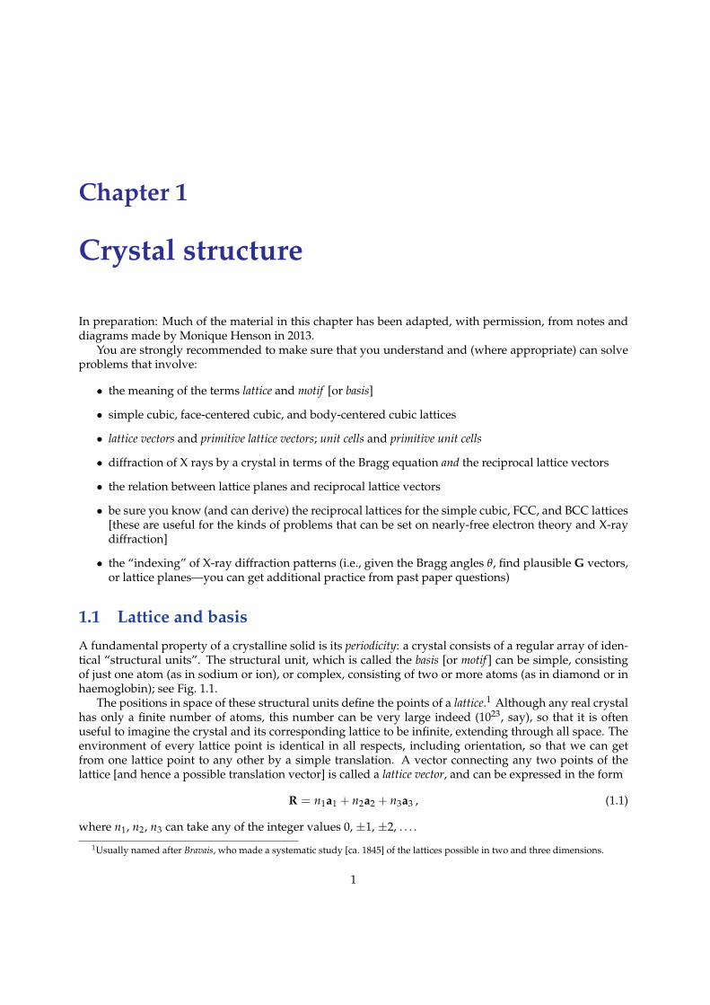
A fundamental property of a crystalline solid is its periodicity: a crystal consists of a regular array of iden-tical “structural units”. The structural unit, which is called the basis [or motif ] can be simple, consistingof just one atom (as in sodium or ion), or complex, consisting of two or more atoms (as in diamond or inhaemoglobin); see Fig. 1.1.
The positions in space of these structural units define the points of a lattice.1 Although any real crystalhas only a finite number of atoms, this number can be very large indeed (1023, say), so that it is oftenuseful to imagine the crystal and its corresponding lattice to be infinite, extending through all space. Theenvironment of every lattice point is identical in all respects, including orientation, so that we can getfrom one lattice point to any other by a simple translation. A vector connecting any two points of thelattice [and hence a possible translation vector] is called a lattice vector, and can be expressed in the form
R = n1a1 + n2a2 + n3a3 , (1.1)
where n1, n2, n3 can take any of the integer values 0, ±1, ±2, . . . .
1Usually named after Bravais, who made a systematic study [ca. 1845] of the lattices possible in two and three dimensions.
1
2 CHAPTER 1. CRYSTAL STRUCTURE
Figure 1.1: An example of a crystal structure. Atoms are represented by grey circles. Three atoms (shadedgreen) make up the motif (or basis) of the structure. Lattice points are indicated by blue dots.
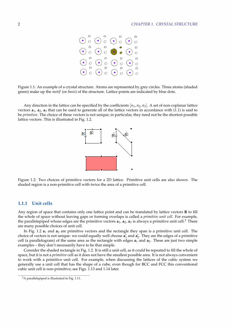
Any direction in the lattice can be specified by the coefficients [n1, n2, n3]. A set of non-coplanar latticevectors a1, a2, a3 that can be used to generate all of the lattice vectors in accordance with (1.1) is said tobe primitive. The choice of these vectors is not unique; in particular, they need not be the shortest possiblelattice vectors. This is illustrated in Fig. 1.2.
Figure 1.2: Two choices of primitive vectors for a 2D lattice. Primitive unit cells are also shown. Theshaded region is a non-primitive cell with twice the area of a primitive cell.
1.1.1 Unit cells
Any region of space that contains only one lattice point and can be translated by lattice vectors R to fillthe whole of space without leaving gaps or forming overlaps is called a primitive unit cell. For example,the parallelepiped whose edges are the primitive vectors a1, a2, a3 is always a primitive unit cell.2 Thereare many possible choices of unit cell.
In Fig. 1.2 a1 and a2 are primitive vectors and the rectangle they span is a primitive unit cell. Thechoice of vectors is not unique: we could equally well choose a′1 and a′2. They are the edges of a primitivecell (a parallelogram) of the same area as the rectangle with edges a1 and a2. These are just two simpleexamples – they don’t necessarily have to be that simple.
Consider the shaded rectangle in Fig. 1.2. It is still a unit cell, as it could be repeated to fill the whole ofspace, but it is not a primitive cell as it does not have the smallest possible area. It is not always convenientto work with a primitive unit cell. For example, when discussing the lattices of the cubic system wegenerally use a unit cell that has the shape of a cube, even though for BCC and FCC this conventionalcubic unit cell is non-primitive; see Figs. 1.13 and 1.14 later.
2A parallelepiped is illustrated in Fig. 1.11.
1.1. LATTICE AND BASIS 3
1.1.2 Crystal symmetry
Lattice symmetries include translation by a lattice vector, discrete rotations (discussed below), and reflec-tions.
Mirror symmetry (reflections)
Mirror symmetry should be familiar enough not to need discussion.
Rotational symmetry
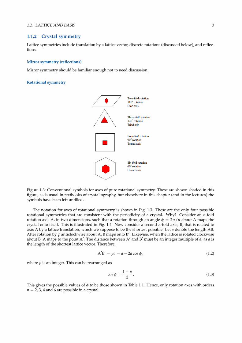
Figure 1.3: Conventional symbols for axes of pure rotational symmetry. These are shown shaded in thisfigure, as is usual in textbooks of crystallography, but elsewhere in this chapter (and in the lectures) thesymbols have been left unfilled.
The notation for axes of rotational symmetry is shown in Fig. 1.3. These are the only four possiblerotational symmetries that are consistent with the periodicity of a crystal. Why? Consider an n-foldrotation axis A, in two dimensions, such that a rotation through an angle φ = 2π/n about A maps thecrystal onto itself. This is illustrated in Fig. 1.4. Now consider a second n-fold axis, B, that is related toaxis A by a lattice translation, which we suppose to be the shortest possible. Let a denote the length AB.After rotation by φ anticlockwise about A, B maps onto B′. Likewise, when the lattice is rotated clockwiseabout B, A maps to the point A′. The distance between A′ and B′ must be an integer multiple of a, as a isthe length of the shortest lattice vector. Therefore,
A′B′ = pa = a− 2a cos φ , (1.2)
where p is an integer. This can be rearranged as
cos φ =1− p
2. (1.3)
This gives the possible values of φ to be those shown in Table 1.1. Hence, only rotation axes with ordersn = 2, 3, 4 and 6 are possible in a crystal.
4 CHAPTER 1. CRYSTAL STRUCTURE
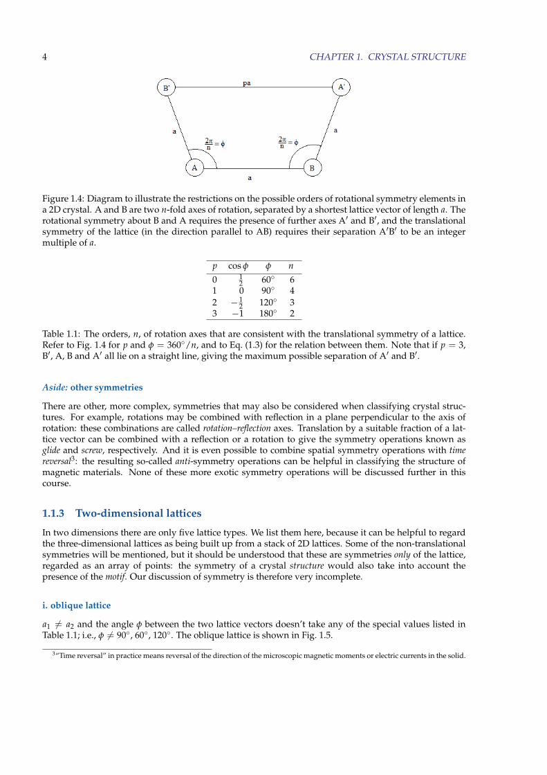
Figure 1.4: Diagram to illustrate the restrictions on the possible orders of rotational symmetry elements ina 2D crystal. A and B are two n-fold axes of rotation, separated by a shortest lattice vector of length a. Therotational symmetry about B and A requires the presence of further axes A′ and B′, and the translationalsymmetry of the lattice (in the direction parallel to AB) requires their separation A′B′ to be an integermultiple of a.
p cos φ φ n0 1
2 60◦ 61 0 90◦ 42 − 1
2 120◦ 33 −1 180◦ 2
Table 1.1: The orders, n, of rotation axes that are consistent with the translational symmetry of a lattice.Refer to Fig. 1.4 for p and φ = 360◦/n, and to Eq. (1.3) for the relation between them. Note that if p = 3,B′, A, B and A′ all lie on a straight line, giving the maximum possible separation of A′ and B′.
Aside: other symmetries
There are other, more complex, symmetries that may also be considered when classifying crystal struc-tures. For example, rotations may be combined with reflection in a plane perpendicular to the axis ofrotation: these combinations are called rotation–reflection axes. Translation by a suitable fraction of a lat-tice vector can be combined with a reflection or a rotation to give the symmetry operations known asglide and screw, respectively. And it is even possible to combine spatial symmetry operations with timereversal3: the resulting so-called anti-symmetry operations can be helpful in classifying the structure ofmagnetic materials. None of these more exotic symmetry operations will be discussed further in thiscourse.
1.1.3 Two-dimensional lattices
In two dimensions there are only five lattice types. We list them here, because it can be helpful to regardthe three-dimensional lattices as being built up from a stack of 2D lattices. Some of the non-translationalsymmetries will be mentioned, but it should be understood that these are symmetries only of the lattice,regarded as an array of points: the symmetry of a crystal structure would also take into account thepresence of the motif. Our discussion of symmetry is therefore very incomplete.
i. oblique lattice
a1 6= a2 and the angle φ between the two lattice vectors doesn’t take any of the special values listed inTable 1.1; i.e., φ 6= 90◦, 60◦, 120◦. The oblique lattice is shown in Fig. 1.5.
3“Time reversal” in practice means reversal of the direction of the microscopic magnetic moments or electric currents in the solid.
1.1. LATTICE AND BASIS 5
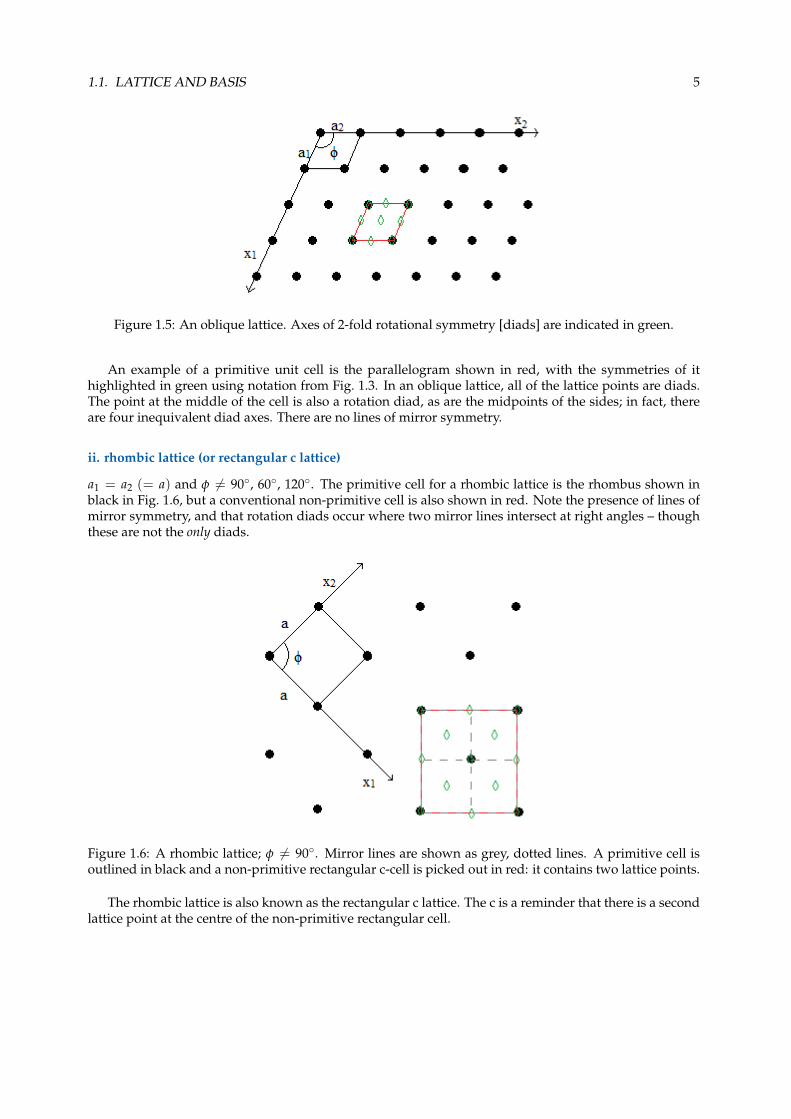
Figure 1.5: An oblique lattice. Axes of 2-fold rotational symmetry [diads] are indicated in green.
An example of a primitive unit cell is the parallelogram shown in red, with the symmetries of ithighlighted in green using notation from Fig. 1.3. In an oblique lattice, all of the lattice points are diads.The point at the middle of the cell is also a rotation diad, as are the midpoints of the sides; in fact, thereare four inequivalent diad axes. There are no lines of mirror symmetry.
ii. rhombic lattice (or rectangular c lattice)
a1 = a2 (= a) and φ 6= 90◦, 60◦, 120◦. The primitive cell for a rhombic lattice is the rhombus shown inblack in Fig. 1.6, but a conventional non-primitive cell is also shown in red. Note the presence of lines ofmirror symmetry, and that rotation diads occur where two mirror lines intersect at right angles – thoughthese are not the only diads.
Figure 1.6: A rhombic lattice; φ 6= 90◦. Mirror lines are shown as grey, dotted lines. A primitive cell isoutlined in black and a non-primitive rectangular c-cell is picked out in red: it contains two lattice points.
The rhombic lattice is also known as the rectangular c lattice. The c is a reminder that there is a secondlattice point at the centre of the non-primitive rectangular cell.
6 CHAPTER 1. CRYSTAL STRUCTURE
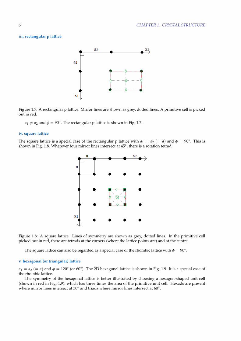
iii. rectangular p lattice
Figure 1.7: A rectangular p lattice. Mirror lines are shown as grey, dotted lines. A primitive cell is pickedout in red.
a1 6= a2 and φ = 90◦. The rectangular p lattice is shown in Fig. 1.7.
iv. square lattice
The square lattice is a special case of the rectangular p lattice with a1 = a2 (= a) and φ = 90◦. This isshown in Fig. 1.8. Wherever four mirror lines intersect at 45◦, there is a rotation tetrad.
Figure 1.8: A square lattice. Lines of symmetry are shown as grey, dotted lines. In the primitive cellpicked out in red, there are tetrads at the corners (where the lattice points are) and at the centre.
The square lattice can also be regarded as a special case of the rhombic lattice with φ = 90◦.
v. hexagonal (or triangular) lattice
a1 = a2 (= a) and φ = 120◦ (or 60◦). The 2D hexagonal lattice is shown in Fig. 1.9. It is a special case ofthe rhombic lattice.
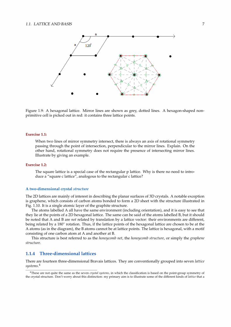
The symmetry of the hexagonal lattice is better illustrated by choosing a hexagon-shaped unit cell(shown in red in Fig. 1.9), which has three times the area of the primitive unit cell. Hexads are presentwhere mirror lines intersect at 30◦ and triads where mirror lines intersect at 60◦.
1.1. LATTICE AND BASIS 7
Figure 1.9: A hexagonal lattice. Mirror lines are shown as grey, dotted lines. A hexagon-shaped non-primitive cell is picked out in red: it contains three lattice points.
Exercise 1.1:
When two lines of mirror symmetry intersect, there is always an axis of rotational symmetrypassing through the point of intersection, perpendicular to the mirror lines. Explain. On theother hand, rotational symmetry does not require the presence of intersecting mirror lines.Illustrate by giving an example.
Exercise 1.2:
The square lattice is a special case of the rectangular p lattice. Why is there no need to intro-duce a “square c lattice”, analogous to the rectangular c lattice?
A two-dimensional crystal structure
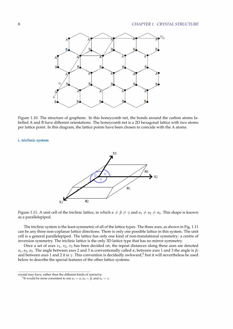
The 2D lattices are mainly of interest in describing the planar surfaces of 3D crystals. A notable exceptionis graphene, which consists of carbon atoms bonded to form a 2D sheet with the structure illustrated inFig. 1.10. It is a single atomic layer of the graphite structure.
The atoms labelled A all have the same environment (including orientation), and it is easy to see thatthey lie at the points of a 2D hexagonal lattice. The same can be said of the atoms labelled B, but it shouldbe noted that A and B are not related by translation by a lattice vector: their environments are different,being related by a 180◦ rotation. Thus, if the lattice points of the hexagonal lattice are chosen to be at theA atoms (as in the diagram), the B atoms cannot be at lattice points. The lattice is hexagonal, with a motifconsisting of one carbon atom at A and another at B.
This structure is best referred to as the honeycomb net, the honeycomb structure, or simply the graphenestructure.
1.1.4 Three-dimensional lattices
There are fourteen three-dimensional Bravais lattices. They are conventionally grouped into seven latticesystems.4
4These are not quite the same as the seven crystal systems, in which the classification is based on the point-group symmetry ofthe crystal structure. Don’t worry about this distinction: my primary aim is to illustrate some of the different kinds of lattice that a
8 CHAPTER 1. CRYSTAL STRUCTURE
Figure 1.10: The structure of graphene. In this honeycomb net, the bonds around the carbon atoms la-belled A and B have different orientations. The honeycomb net is a 2D hexagonal lattice with two atomsper lattice point. In this diagram, the lattice points have been chosen to coincide with the A atoms.
i. triclinic system
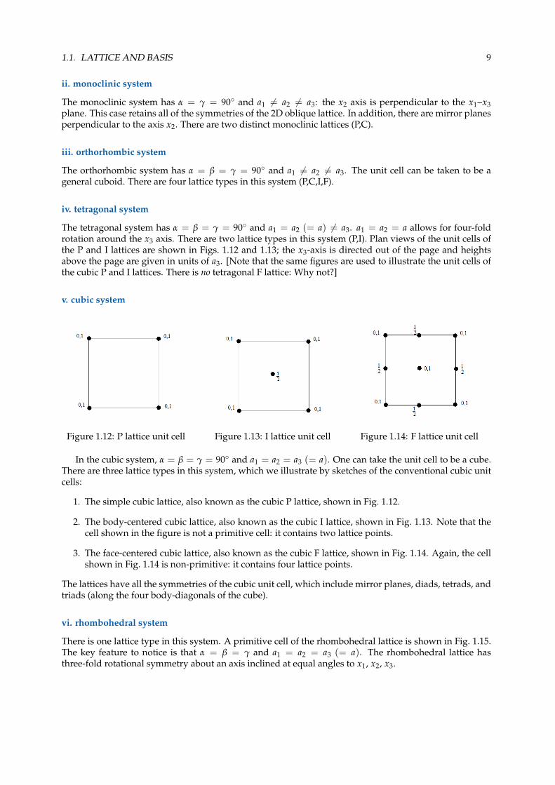
Figure 1.11: A unit cell of the triclinic lattice, in which α 6= β 6= γ and a1 6= a2 6= a3. This shape is knownas a parallelepiped.
The triclinic system is the least symmetric of all of the lattice types. The three axes, as shown in Fig. 1.11can be any three non-coplanar lattice directions. There is only one possible lattice in this system. The unitcell is a general parallelepiped. The lattice has only one kind of non-translational symmetry: a centre ofinversion symmetry. The triclinic lattice is the only 3D lattice type that has no mirror symmetry.
Once a set of axes x1, x2, x3 has been decided on, the repeat distances along these axes are denoteda1, a2, a3. The angle between axes 2 and 3 is conventionally called α; between axes 1 and 3 the angle is β;and between axes 1 and 2 it is γ. This convention is decidedly awkward,5 but it will nevertheless be usedbelow to describe the special features of the other lattice systems.
crystal may have, rather than the different kinds of symmetry.5It would be more consistent to use α1 = α, α2 = β, and α3 = γ.
1.1. LATTICE AND BASIS 9
ii. monoclinic system
The monoclinic system has α = γ = 90◦ and a1 6= a2 6= a3: the x2 axis is perpendicular to the x1–x3plane. This case retains all of the symmetries of the 2D oblique lattice. In addition, there are mirror planesperpendicular to the axis x2. There are two distinct monoclinic lattices (P,C).
iii. orthorhombic system
The orthorhombic system has α = β = γ = 90◦ and a1 6= a2 6= a3. The unit cell can be taken to be ageneral cuboid. There are four lattice types in this system (P,C,I,F).
iv. tetragonal system
The tetragonal system has α = β = γ = 90◦ and a1 = a2 (= a) 6= a3. a1 = a2 = a allows for four-foldrotation around the x3 axis. There are two lattice types in this system (P,I). Plan views of the unit cells ofthe P and I lattices are shown in Figs. 1.12 and 1.13; the x3-axis is directed out of the page and heightsabove the page are given in units of a3. [Note that the same figures are used to illustrate the unit cells ofthe cubic P and I lattices. There is no tetragonal F lattice: Why not?]
v. cubic system
Figure 1.12: P lattice unit cell Figure 1.13: I lattice unit cell Figure 1.14: F lattice unit cell
In the cubic system, α = β = γ = 90◦ and a1 = a2 = a3 (= a). One can take the unit cell to be a cube.There are three lattice types in this system, which we illustrate by sketches of the conventional cubic unitcells:
1. The simple cubic lattice, also known as the cubic P lattice, shown in Fig. 1.12.
2. The body-centered cubic lattice, also known as the cubic I lattice, shown in Fig. 1.13. Note that thecell shown in the figure is not a primitive cell: it contains two lattice points.
3. The face-centered cubic lattice, also known as the cubic F lattice, shown in Fig. 1.14. Again, the cellshown in Fig. 1.14 is non-primitive: it contains four lattice points.
The lattices have all the symmetries of the cubic unit cell, which include mirror planes, diads, tetrads, andtriads (along the four body-diagonals of the cube).
vi. rhombohedral system
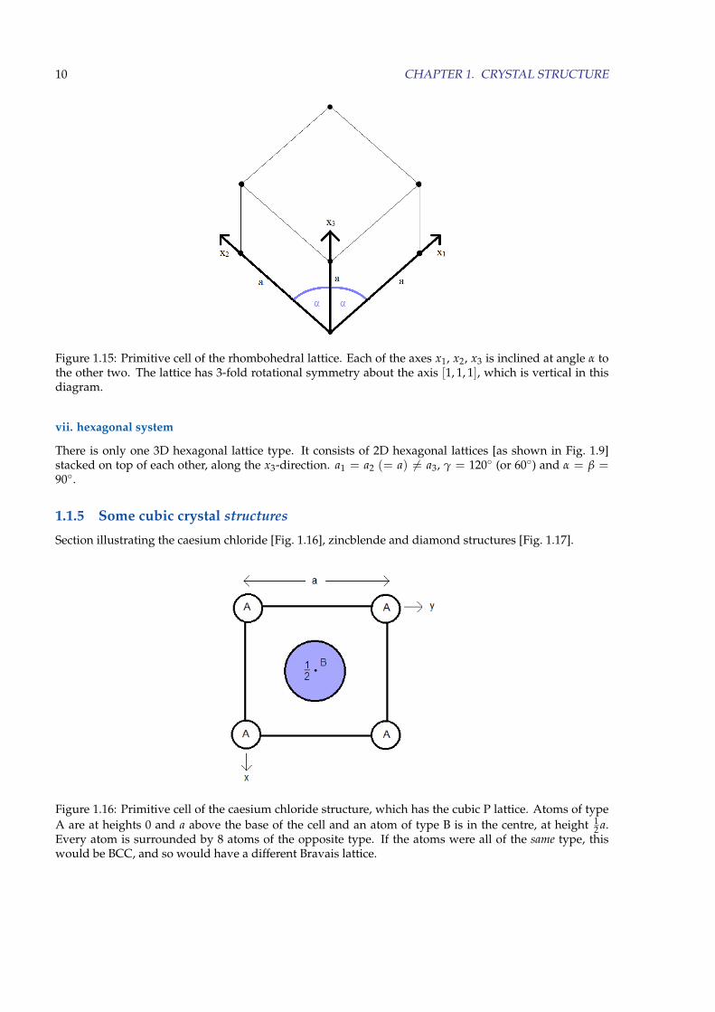
There is one lattice type in this system. A primitive cell of the rhombohedral lattice is shown in Fig. 1.15.The key feature to notice is that α = β = γ and a1 = a2 = a3 (= a). The rhombohedral lattice hasthree-fold rotational symmetry about an axis inclined at equal angles to x1, x2, x3.
10 CHAPTER 1. CRYSTAL STRUCTURE
Figure 1.15: Primitive cell of the rhombohedral lattice. Each of the axes x1, x2, x3 is inclined at angle α tothe other two. The lattice has 3-fold rotational symmetry about the axis [1, 1, 1], which is vertical in thisdiagram.
vii. hexagonal system
There is only one 3D hexagonal lattice type. It consists of 2D hexagonal lattices [as shown in Fig. 1.9]stacked on top of each other, along the x3-direction. a1 = a2 (= a) 6= a3, γ = 120◦ (or 60◦) and α = β =90◦.
1.1.5 Some cubic crystal structures
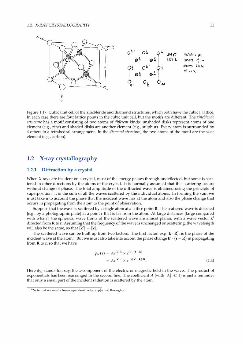
Section illustrating the caesium chloride [Fig. 1.16], zincblende and diamond structures [Fig. 1.17].
Figure 1.16: Primitive cell of the caesium chloride structure, which has the cubic P lattice. Atoms of typeA are at heights 0 and a above the base of the cell and an atom of type B is in the centre, at height 1
2 a.Every atom is surrounded by 8 atoms of the opposite type. If the atoms were all of the same type, thiswould be BCC, and so would have a different Bravais lattice.
1.2. X-RAY CRYSTALLOGRAPHY 11
Figure 1.17: Cubic unit cell of the zincblende and diamond structures, which both have the cubic F lattice.In each case there are four lattice points in the cubic unit cell, but the motifs are different. The zincblendestructure has a motif consisting of two atoms of different kinds: unshaded disks represent atoms of oneelement (e.g., zinc) and shaded disks are another element (e.g., sulphur). Every atom is surrounded by4 others in a tetrahedral arrangement. In the diamond structure, the two atoms of the motif are the sameelement (e.g., carbon).
1.2 X-ray crystallography
1.2.1 Diffraction by a crystal
When X rays are incident on a crystal, most of the energy passes through undeflected, but some is scat-tered in other directions by the atoms of the crystal. It is normally assumed that this scattering occurswithout change of phase. The total amplitude of the diffracted wave is obtained using the principle ofsuperposition: it is the sum of all the waves scattered by the individual atoms. In forming the sum wemust take into account the phase that the incident wave has at the atom and also the phase change thatoccurs in propagating from the atom to the point of observation.
Suppose that the wave is scattered by a single atom at a lattice point R. The scattered wave is detected[e.g., by a photographic plate] at a point r that is far from the atom. At large distances [large comparedwith what?] the spherical wave fronts of the scattered wave are almost planar, with a wave vector k′
directed from R to r. Assuming that the frequency of the wave is unchanged on scattering, the wavelengthwill also be the same, so that |k′| = |k|.
The scattered wave can be built up from two factors. The first factor, exp[ik · R], is the phase of theincident wave at the atom.6 But we must also take into accout the phase change k′ · (r−R) in propagatingfrom R to r, so that we have
ψsc(r) = Aeik·R × eik′ ·(r−R)
= Aeik′ ·r × e−i(k′−k)·R. (1.4)
Here ψsc stands for, say, the x-component of the electric or magnetic field in the wave. The product ofexponentials has been rearranged in the second line. The coefficient A (with |A| � 1) is just a reminderthat only a small part of the incident radiation is scattered by the atom.
6Note that we omit a time-dependent factor exp[−iωt] throughout.
12 CHAPTER 1. CRYSTAL STRUCTURE
Finally we sum the individual waves (1.4) over all the atoms of the crystal to obtain the total scatteredwave:
ψtotsc (r) = Aeik′ ·r ×∑
Re−i(k′−k)·R. (1.5)
The first factor here simply expresses the fact that the scattered wave has wave vector k′, but the secondfactor
∑R
e−i(k′−k)·R (1.6)
depends crucially on the particular lattice and it determines whether waves will be scattered strongly inthe direction k′. The scattered wave is large only when all of the terms in (1.5) have the same phase. Fora given incident wave with wave vector k this can happen only for a discrete set of outgoing waves withwave vectors k′. For every pair of pair of terms in the sum (1.6) we have
e−i(k′−k)·R1 = e−i(k′−k)·R2 , or ei(k′−k)·(R1−R2) = 1 . (1.7)
But R1 − R2 is just a lattice vector, so that the condition for constructive interference becomes
ei(k′−k)·R = 1 (1.8)
for every vector R of the lattice. The solution of this equation will lead us to the concept of a reciprocallattice.
1.2.2 The reciprocal lattice
We need to solve Eq. (1.8), the condition for constructive intereference, to obtain the wave vectors k′.Writing the difference k′ − k as G, we have
eiG·R = 1 or G · R = 2πP , (1.9)
where P is an integer [positive, negative or zero], and R is any lattice vector. In particular, the condition(1.9) must be satisfied for a set of primitive lattice vectors,
G · a1 = 2πp1 , G · a2 = 2πp2 , G · a3 = 2πp3 , (1.10)
where p1, p2, p3 are all integers. The last three equations, the Laue equations, can be solved for any latticetype.
Before tackling the general case it is helpful first to look at the simpler case of the orthorhombic Plattice, for which we can take the primitive vectors a1, a2, a3 to be orthogonal. In this case, a1 = a1x,a2 = a2y, a3 = a3z, so that the Laue equations (1.10) reduce to
Gx = 2πp1/a1 , Gy = 2πp2/a2 , Gx = 2πp3/a3 . (1.11)
The solutionsG = 2π (p1x/a1 + p2y/a2 + p3z/a3) (1.12)
define the points of an orthorhombic reciprocal lattice with repeat distances b1 = 2π/a1, b2 = 2π/a2,b3 = 2π/a3 along the coordinate axes. Note that these repeat distances are not the same as in the originallattice; in fact, they have the dimensions of reciprocal length. To emphasize this distinction, the lattice ofthe original crystal structure is often called the direct lattice.
General solution of the Laue equations
The general solution of (1.10) for non-orthogonal primitive vectors a1, a2, a3 of the direct lattice can bewritten as
G = p1b1 + p2b2 + p3b3 , (1.13)where the primitive vectors b1, b2, b3 of the reciprocal lattice are given by
b1 =2π a2 × a3
a1 · [a2 × a3], b2 =
2π a3 × a1
a1 · [a2 × a3], b3 =
2π a1 × a2
a1 · [a2 × a3]. (1.14)
1.2. X-RAY CRYSTALLOGRAPHY 13
Exercise 1.3:
Verify that a reciprocal vector given by (1.13) and (1.14) satisfies Eq. (1.9) for any R of the formn1a1 + n2a2 + n3a3, where P = p1n1 + p2n2 + p3n3 in Eq. (1.9).
Geometrically, the scalar triple product a1 · [a2 × a3] appearing in the denominators in Eq. (1.14) rep-resents the volume of a parallelepiped with edges a1, a2, a3; i.e., it is the volume of the primitive unitcell. The products in the numerators, e.g. a1 × a2, are the vector areas of the faces of this cell. In mag-nitude, therefore, the vectors bi are 2π times the reciprocal altitudes of the parallelepiped, and they areperpendicular to its faces.
Notation for vectors of the direct and reciprocal lattices
Once a set of primitive vectors a1, a2, a3 has been chosen, vectors of the direct lattice are often specifiedsimply by giving the coefficients of the ai in square brackets:
R = n1a1 + n2a2 + n3a3 ≡ [n1, n2, n3] . (1.15)
Similarly, reciprocal lattice vectors are specified by giving the coefficients of the vectors bi in round brack-ets:
G = p1b1 + p2b2 + p3b3 ≡ (p1, p2, p3) . (1.16)
This distinction between square and round brackets is not always observed by physicists, but it is a con-vention that we shall use throughout this course.
In the above notation, crystallographers like to omit the commas in cases where there would be noambiguity and to use overbars to indicate negative coefficients. For example, (132) means exactly thesame thing as (1,−3, 2). This convention can save a little space in diagrams and tables.7
1.2.3 Reciprocal lattice vectors and lattice planes
There is a very close connection between reciprocal lattice vectors and lattice planes, which is illustratedin Fig. 1.20. We imagine a plane wave exp[iG · r] in a crystal. By the definition (1.9) of reciprocal latticevectors, this wave would have the same phase G · r = 0 (modulo 2π) at every lattice point r = R. Everylattice plane perpendicular to G is therefore a wavefront of the wave exp[iG · r]. There may, however,be additional wavefronts that lie between the lattice planes, as shown in the diagram. It follows thatthe spacing of the lattice planes must be an integer multiple of the wavelength λG (= 2π/|G|) of thisfictitious wave:
d = nλG = n× 2π
|G| , where n = 1, 2, 3, . . . . (1.17)
Let us write G = nGs, where Gs = (l1, l2, l3) is the shortest reciprocal lattice vector in the direction ofG = (p1, p2, p3) and n is the greatest common divisor of p1, p2, p3. Then
d =2π
|Gs|=
2π
|l1b1 + l2b2 + l3b3|. (1.18)
The integers l1, l2, l3 are called the Miller indices of the lattice planes perpendicular to G.Equation (1.18) is a very easy way to calculate the interplanar spacing from the length of the reciprocal
lattice vector Gs = (l1, l2, l3), and it is well worth understanding it fully.
7Don’t feel obliged to follow the convention of omitting commas and using overbars.
14 CHAPTER 1. CRYSTAL STRUCTURE
Aside: Alternative definition of the Miller indices
Last year, the Miller indices of a lattice plane were introduced to you in a different way, by using the recip-rocals of the plane’s intercepts on the coordinate axes. We should check that our approach is equivalent.
Any position vector r can be written in the form
r = x1a1 + x2a2 + x3a3 ;
the expansion is analogous to Eq. (1.1), but the dimensionless coefficients x1, x2, x3 need not be integers.Consider a family of lattice planes specified by the reciprocal lattice vector Gs = (l1, l2, l3), where theintegers li have no common divisor greater than 1. The equation of the lattice plane closest to the origin(but not passing through it) is Gs · r = 2π. Then, in terms of the xi, this becomes
Gs · r = 2π(l1x1 + l2x2 + l3x3) = 2π .
By setting x2 = x3 = 0 we find that the plane crosses the x1-axis at x1 = 1/l1, where the distance ismeasured in units of a1. Similarly, the intercepts on the x2- and x3-axes are 1/l2 and 1/l3.
Hence, the Miller indices l1, l2, l3 of a lattice place could be defined as the reciprocals of its interceptson the axes x1, x2, x3.
1.2.4 The Bragg construction
We have found above that the condition for diffraction is k′−k = G, where G is a reciprocal lattice vector.W. L. Bragg [in 1913] used this result to find an alternative formulation of the diffraction condition.
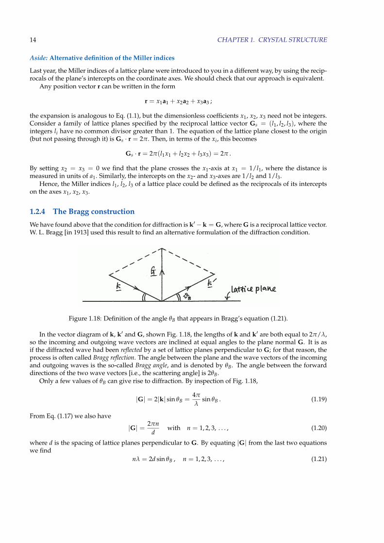
Figure 1.18: Definition of the angle θB that appears in Bragg’s equation (1.21).
In the vector diagram of k, k′ and G, shown Fig. 1.18, the lengths of k and k′ are both equal to 2π/λ,so the incoming and outgoing wave vectors are inclined at equal angles to the plane normal G. It is asif the diffracted wave had been reflected by a set of lattice planes perpendicular to G; for that reason, theprocess is often called Bragg reflection. The angle between the plane and the wave vectors of the incomingand outgoing waves is the so-called Bragg angle, and is denoted by θB. The angle between the forwarddirections of the two wave vectors [i.e., the scattering angle] is 2θB.
Only a few values of θB can give rise to diffraction. By inspection of Fig. 1.18,
|G| = 2|k| sin θB =4π
λsin θB . (1.19)
From Eq. (1.17) we also have
|G| = 2πnd
with n = 1, 2, 3, . . . , (1.20)
where d is the spacing of lattice planes perpendicular to G. By equating |G| from the last two equationswe find
nλ = 2d sin θB , n = 1, 2, 3, . . . , (1.21)
1.2. X-RAY CRYSTALLOGRAPHY 15
which is Bragg’s equation; it is fully equivalent to the vector condition k′ − k = G. Since the left-hand sideof (1.21) cannot be less than λ and the sine function cannot be greater than unity, Bragg’s equation showsthat for diffraction to occur, the wavelength λ must be less than twice the spacing between lattice planes.
Bragg’s equation is often interpreted [and derived, sort of] as the condition for constructive inter-ference of waves “reflected” by neighbouring lattice planes: the path difference for the two waves is amultiple n of the wavelength. In this context, n is often called the order of diffraction, by analogy withdiffraction by a ruled grating or a pair of Young’s slits.
As an example we consider a simple cubic solid with lattice parameter a. A diffracted wave corre-sponding to G = (222) = 2 · (111) is a second-order (n = 2) reflection from the (111) planes of the directlattice. These planes are perpendicular to the [111] direction, with spacing d111 = a/
√3. [Check this.] It
would normally be called the (222) reflection, with or without the round brackets, as this tells us both theorder of reflection and the planes involved. Similarly, (630) would denote the third-order reflection fromthe (210) planes (spacing d210 = a/
√5).
In practice, it is not very easy to apply Bragg’s equation without having recourse to the reciprocallattice: it is hard to visualize all the sets of planes and the geometrical relationships between them, and theinterplanar spacings are, in any case, most easily calculated using Eq. (1.18). Once the initial conceptualproblems have been overcome, it is often simpler to use k′ − k = G directly, since this only requires us tovisualize the points of the reciprocal lattice.
1.2.5 Structure factor
In Sec. 1.2.1 we obtained the amplitude for a a wave diffracted by a crystal in the case where there is onlyone atom per lattice point. How are the results changed if the structural motif consists of more than oneatom?
If the motif contains M atoms labelled j = 1, 2, . . ., M, the atoms associated with a particular latticepoint R can be taken to have positions R + rj. For example, if R is taken to be at one corner of the unitcell, the vectors rj are the positions of the atoms within the unit cell, measured relative to that corner.
The sum in (1.5) can be generalized to
ψtotsc (r) = Aeik′ ·r ×∑
R
{ M
∑j=1
f j e−i(k′−k)·(R+rj)}
= Aeik′ ·r ×∑R
e−i(k′−k)·R ×M
∑j=1
f j e−i(k′−k)·rj , (1.22)
where the factors f j (discussed shortly) take account of the fact that the atoms need not be all of the samekind, and so may scatter differently. The second factor in (1.22), involving a sum over lattice points R, hasbeen discussed following (1.6); it is large only if k′ − k is a reciprocal lattice vector. Accordingly, the lastfactor, involving the sum over j, needs to be considered only for those special values k′ − k = G:
S(G) =M
∑j=1
f j e−iG·rj ; (1.23)
S(G) is known as the structure factor. Equation (1.22) is an expression for the (complex) amplitude of thewave scattered by the crystal; the X-ray intensity is proportional to the square of the amplitude, so that thevarious diffracted waves will have intensities proportional to |S(G)|2.
The atomic form factors f j, which determine the strength of scattering by individual atoms, are givenby
f j =∫
atom jnj(r) e−iG·r d3r , (1.24)
where nj(r) is the number density of electrons in atom j and the origin of coordinates for the integrationis taken to be the centre of the atom. Atomic form factors decrease with increasing |G|, so that diffractiontends to be strongest for small values of the indices p1, p2, p3.
16 CHAPTER 1. CRYSTAL STRUCTURE
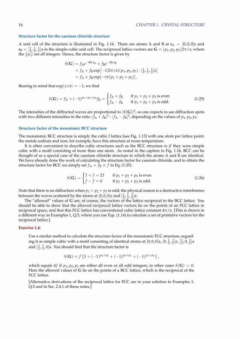
Structure factor for the caesium chloride structure
A unit cell of the structure is illustrated in Fig. 1.16. There are atoms A and B at rA = [0, 0, 0]a andrB = [ 1
2 , 12 , 1
2 ]a in the simple-cubic unit cell. The reciprocal lattice vectors are G = (p1, p2, p3)2π/a, wherethe {pi} are all integers. Hence, the structure factor is given by
S(G) = fAe−iG·rA + fBe−iG·rB
= fA + fB exp[−i(2π/a)(p1, p2, p3) · [ 1
2 , 12 , 1
2 ]a]
= fA + fB exp[−iπ(p1 + p2 + p3)] .
Bearing in mind that exp[±iπ] = −1, we find
S(G) = fA + (−1)p1+p2+p3 fB =
{fA + fB if p1 + p2 + p3 is evenfA − fB if p1 + p2 + p3 is odd.
(1.25)
The intensities of the diffracted waves are proportional to |S(G)|2, so one expects to see diffraction spotswith two different intensities in the ratio | fA + fB|2 : | fA − fB|2, depending on the values of p1, p2, p3.
Structure factor of the monatomic BCC structure
The monatomic BCC structure is simply the cubic I lattice [see Fig. 1.13] with one atom per lattice point;the metals sodium and iron, for example, have this structure at room temperature.
It is often convenient to describe cubic structures such as the BCC structure as if they were simplecubic with a motif consisting of more than one atom. As noted in the caption to Fig. 1.16, BCC can bethought of as a special case of the caesium chloride structure in which the atoms A and B are identical.We have already done the work of calculating the structure factor for caesium chloride, and to obtain thestructure factor for BCC we simply set fA = fB ≡ f in Eq. (1.25):
S(G) =
{f + f = 2 f if p1 + p2 + p3 is evenf − f = 0 if p1 + p2 + p3 is odd.
(1.26)
Note that there is no diffraction when p1 + p2 + p3 is odd; the physical reason is a destructive interferencebetween the waves scattered by the atoms at [0, 0, 0]a and [ 1
2 , 12 , 1
2 ]a.The “allowed” values of G are, of course, the vectors of the lattice reciprocal to the BCC lattice. You
should be able to show that the allowed reciprocal lattice vectors lie on the points of an FCC lattice inreciprocal space, and that this FCC lattice has conventional cubic lattice constant 4π/a. [This is shown ina different way in Examples 1, Q.5, where you use Eqs. (1.14) to calculate a set of primitive vectors for thereciprocal lattice.]
Exercise 1.4:
Use a similar method to calculate the structure factor of the monatomic FCC structure, regard-ing it as simple cubic with a motif consisting of identical atoms at [0, 0, 0]a, [0, 1
2 , 12 ]a, [ 1
2 , 0, 12 ]a
and [ 12 , 1
2 , 0]a. You should find that the structure factor is
S(G) = f{
1 + (−1)p2+p3 + (−1)p3+p1 + (−1)p1+p2}
,
which equals 4 f if p1, p2, p3 are either all even or all odd integers; in other cases S(G) = 0.Here the allowed values of G lie on the points of a BCC lattice, which is the reciprocal of theFCC lattice.
[Alternative derivations of the reciprocal lattice for FCC are in your solution to Examples 1,Q.5 and in Sec. 2.4.1 of these notes.]
1.2. X-RAY CRYSTALLOGRAPHY 17
1.2.6 Further geometry of diffraction
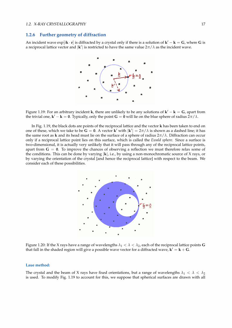
An incident wave exp[ik · r] is diffracted by a crystal only if there is a solution of k′ − k = G, where G isa reciprocal lattice vector and |k′| is restricted to have the same value 2π/λ as the incident wave.
Figure 1.19: For an arbitrary incident k, there are unlikely to be any solutions of k′ − k = G, apart fromthe trivial one, k′ − k = 0. Typically, only the point G = 0 will lie on the blue sphere of radius 2π/λ.
In Fig. 1.19, the black dots are points of the reciprocal lattice and the vector k has been taken to end onone of these, which we take to be G = 0. A vector k′ with |k′| = 2π/λ is shown as a dashed line; it hasthe same root as k and its head must lie on the surface of a sphere of radius 2π/λ. Diffraction can occuronly if a reciprocal lattice point lies on this surface, which is called the Ewald sphere. Since a surface istwo-dimensional, it is actually very unlikely that it will pass through any of the reciprocal lattice points,apart from G = 0. To improve the chances of observing a reflection we must therefore relax some ofthe conditions. This can be done by varying |k|, i.e., by using a non-monochromatic source of X rays, orby varying the orientation of the crystal [and hence the reciprocal lattice] with respect to the beam. Weconsider each of these possibilities.
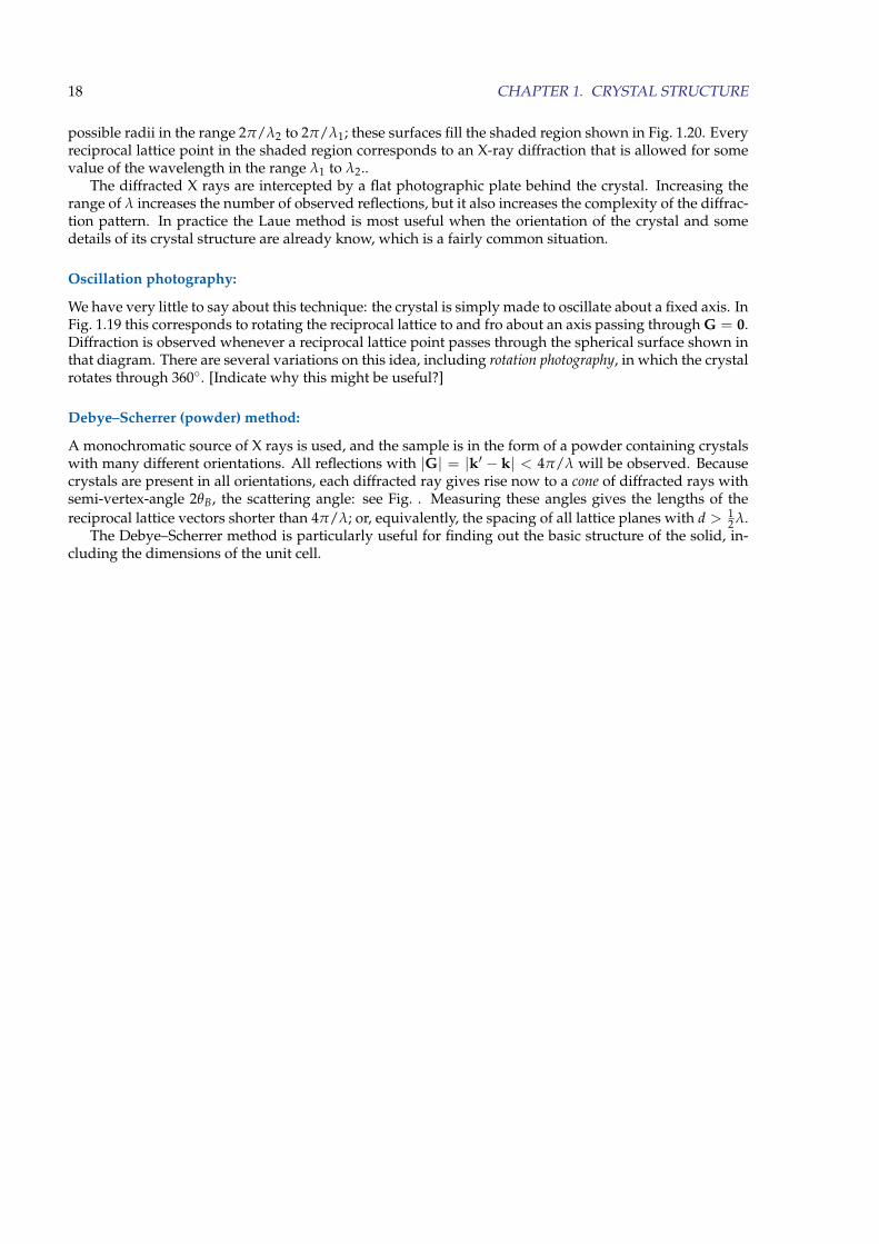
Figure 1.20: If the X rays have a range of wavelengths λ1 < λ < λ2, each of the reciprocal lattice points Gthat fall in the shaded region will give a possible wave vector for a diffracted wave, k′ = k + G.
Laue method:
The crystal and the beam of X rays have fixed orientations, but a range of wavelengths λ1 < λ < λ2is used. To modify Fig. 1.19 to account for this, we suppose that spherical surfaces are drawn with all
18 CHAPTER 1. CRYSTAL STRUCTURE
possible radii in the range 2π/λ2 to 2π/λ1; these surfaces fill the shaded region shown in Fig. 1.20. Everyreciprocal lattice point in the shaded region corresponds to an X-ray diffraction that is allowed for somevalue of the wavelength in the range λ1 to λ2..
The diffracted X rays are intercepted by a flat photographic plate behind the crystal. Increasing therange of λ increases the number of observed reflections, but it also increases the complexity of the diffrac-tion pattern. In practice the Laue method is most useful when the orientation of the crystal and somedetails of its crystal structure are already know, which is a fairly common situation.
Oscillation photography:
We have very little to say about this technique: the crystal is simply made to oscillate about a fixed axis. InFig. 1.19 this corresponds to rotating the reciprocal lattice to and fro about an axis passing through G = 0.Diffraction is observed whenever a reciprocal lattice point passes through the spherical surface shown inthat diagram. There are several variations on this idea, including rotation photography, in which the crystalrotates through 360◦. [Indicate why this might be useful?]
Debye–Scherrer (powder) method:
A monochromatic source of X rays is used, and the sample is in the form of a powder containing crystalswith many different orientations. All reflections with |G| = |k′ − k| < 4π/λ will be observed. Becausecrystals are present in all orientations, each diffracted ray gives rise now to a cone of diffracted rays withsemi-vertex-angle 2θB, the scattering angle: see Fig. . Measuring these angles gives the lengths of thereciprocal lattice vectors shorter than 4π/λ; or, equivalently, the spacing of all lattice planes with d > 1
2 λ.The Debye–Scherrer method is particularly useful for finding out the basic structure of the solid, in-
cluding the dimensions of the unit cell.
Chapter 2
Electrons in crystals
2.1 Summary of free-electron theory, etc.
Not yet formatted for LATEX. Your notes from PHYS20252, PHYS30151 and J. Pearson’s notes, availableonline, contain all the material needed on free electrons.
To cut down the number of broken cross-references within this document, we note here that the radiusof the Fermi sphere (or Fermi wave vector) kF and the electron number density n are related by
kF3 = 3π2n or n =
kF3
3π2 . (2.1)
2.2 Electrons in a periodic potential
We suppose that an electron in a perfect crystal moves in a spatially periodic field of force due to theions and the averaged effect of all the electrons. This is an idealization because the Coulomb repulsionbetween electrons tends to keep them apart (their motion is correlated); nevertheless, it is still the startingpoint for understanding the behaviour of electrons in solids and it is remarkably successful in practice.
2.2.1 Bloch’s theorem
Electrons moving in a periodic potential V(r) are often called Bloch electrons. Their wave functions obeythe Schrodinger equation
− h2
2m∇2ψi(r) + V(r)ψi(r) = Eiψi(r). (2.2)
Some of the most important and most general properties of the solutions ψi(r) of (2.2) depend only on theperiodicity of the potential: V(r) = V(r + R), where R is any vector (a lattice vector) connecting similarpoints of the crystal lattice.
First we notice that if ψi(r) is a solution of (2.2) having energy Ei, then so too is ψi(r + R): the twofunctions are related by a constant factor, ψi(r + R) = c(R)ψi(r). The modulus |c(R)| will be unitysince the probability |ψi(r)|2 of finding the electron in the neighbourhood of r should be the same as theprobability |ψi(r + R)|2 for finding it near r + R, where the local environment is identical. The factor c(R)will also obey c(R + R′) = c(R) c(R′), because translation by R + R′ is identical to successive translationsby lattice vectors R and R′. Only a complex exponential function of R has both properties: the dependenceof the wave function on R reduces to a factor exp[ik · R],
ψk(r + R) = eik·Rψk(r). (2.3)
19
20 CHAPTER 2. ELECTRONS IN CRYSTALS
This is Bloch’s theorem.1 It enables us to write the wave function in the form
ψk(r) = eik·ruk(r), (2.4)
where uk(r) is a periodic function of r, uk(r) = uk(r + R).
Exercise 2.1:
Show that the results (2.3) and (2.4) are equivalent.
The property (2.3) is also possessed by the free-electron wave function
ψk(r) = eik·r,
where hk is the momentum of the electron. Although for an electron in a lattice the wave function is not aplane wave and the momentum is not conserved (it cannot be, because the electron is subject to forces dueto the ions and the other electrons), it is worth noting that the electron is still characterized by a constantvector k: hk is called the crystal momentum of the electron.
Fourier series in three dimensions
The potential V(r) and the function uk(r) appearing in (2.4) are both periodic in space: V(r + R) = V(r),where R is a lattice vector. In PHYS20171, you learned that periodic functions of one variable can beexpanded in a Fourier series. The complex exponential functions exp[2πinx/a] have period a and can beused as a basis for expanding a periodic function f (x) = f (x + a):
f (x) =∞
∑n=−∞
cn e2πinx/a, where cn =1a
∫ a
0e−2πinx/a f (x) dx. (2.5)
We can do the same for a periodic function in three dimensions. We have already discussed the planewaves that have the same periodicity as the crystal lattice. They are the functions exp[iG · r], where G isa reciprocal lattice vector. By analogy with (2.5) we can write
V(r) = ∑G
VG eiG·r, where VG =1
vcell
∫cell
e−iG·r V(r) d3r , (2.6)
where the sum over G in the Fourier representation of V(r) includes all reciprocal lattice vectors, and theformula for the Fourier coefficient (which we are unlikely to use in this course) involves an integral overa primitive unit cell of the crystal lattice.
If f (x) is a real function of x, the coefficients cn may still be complex, but satisfy the symmetry propertycn∗ = c−n, which follows directly from the formula used to calculate them. Similarly, it should be easy
for you to see that VG∗ = V−G.
Representation of the wave function in terms of plane waves
By using the results described in the preceding section, we can write the periodic function uk(r) as aFourier series,
uk(r) = ∑G
CG eiG·r,
so that ψk(r) can be writtenψk(r) = eik·r uk(r) = ∑
GCG ei(k+G)·r. (2.7)
1We have argued here only for the plausibility of (2.3). The books by Kittel and Ashcroft and Mermin give proofs based on theFourier representations of ψk(r) and V(r) discussed later in this section.
2.2. ELECTRONS IN A PERIODIC POTENTIAL 21
This last expression shows explicitly that ψk is sum of many plane waves, and so is not a momentumeigenstate; this confirms that the crystal momentum hk is not the momentum of the electron. In fact, ameasurement of the momentum of the electron could give any of the results h(k + G) and the squaredcoefficients |CG|2 give the relative probabilities of obtaining these different results.
Nevertheless, a measurement of the momentum cannot give just any value. A completely generalfunction, satisfying periodic boundary conditions at the surface of a crystal of volume L3, can be expandedas a Fourier series
ψ(r) = ∑q
Fq eiq·r, where Fq =1L3
∫crystal
e−iq·r ψ(r) d3r . (2.8)
Comparison of (2.7) and (2.8) shows that ψk(r) contains only a tiny fraction of the possible waves withwave vector q; namely, the waves with q = k + G. For consistency with the notation used in (2.8) weshall in future write the expansion of ψk in the form
ψk(r) = ∑G
Fk+G ei(k+G)·r. (2.9)
The form of the last expression makes it clear that ψk is identical to ψk+K, where K is any reciprocallattice vector. Because ψk has the periodicity of the reciprocal lattice, the same is true for any observableproperty of the electron, such as its energy, E(k) = E(k + K).
Exercise 2.2:
The periodicity of ψk, regarded as a function of k, follows from the fact that the summand in(2.9) depends only on k + G. If the periodicity is not obvious to you, prove it by replacing kby k + K on both sides of (2.9). Change the variable of summation to G′ = G + K, and notethat a sum over all G of the reciprocal lattice is equivalent to a sum over all G′.
2.2.2 Brillouin zones
Given that any physical property of an electron has the periodicity of the reciprocal lattice, it is only evernecessary to plot the energy in a primitive unit cell of reciprocal space. Any primitive unit cell would dofor this, but a conventional choice of unit cell is the so-called first Brillouin zone, which is the set of vectorsk that are closer to k = 0 than to any other reciprocal lattice point G 6= 0.
For example, consider a crystal with a simple-cubic lattice, with lattice constant a. In this case, thereciprocal lattice is also a simple-cubic lattice with lattice constant 2π/a. The first Brillouin zone is then acube of side 2π/a whose faces are planes bisecting (at right-angles) the shortest reciprocal lattice vectors(100)2π/a, (010)2π/a and (001)2π/a.
Second, third, and nth Brillouin zones
The perpendicular bisectors of the reciprocal lattice vectors G 6= 0 are sometimes called zone boundaries orBragg planes.2 Given the concept of a zone boundary, the first Brillouin zone could be defined as the set ofpoints k that can be reached from k = 0 without crossing a zone boundary.
Higher Brillouin zones can be defined in a similar way. The second Brillouin zone is the set of ks thatcan be reached from k = 0 by crossing exactly one zone boundary, and the third Brillouin zone is the setthat can be reached by crossing two—and no fewer than two—zone boundaries. Each of these zones is aprimitive unit cell of reciprocal space. Generalizing this idea, the nth Brillouin zone is the set of ks thatcan be reached from k = 0 by crossing n− 1 (and no fewer than n− 1) zone boundaries. As n increases,the shapes of the zones become increasingly complex; this is illustrated in Figure 2.1 for the case of atwo-dimensional square lattice.
2The term “Bragg plane” is avoided in these notes because there is a chance of confusing it with the lattice planes responsible forBragg reflection. Zone boundaries (and Bragg planes) are planes in reciprocal space; lattice planes, of course, are planes of latticepoints in direct space, i.e., in r-space.
22 CHAPTER 2. ELECTRONS IN CRYSTALS
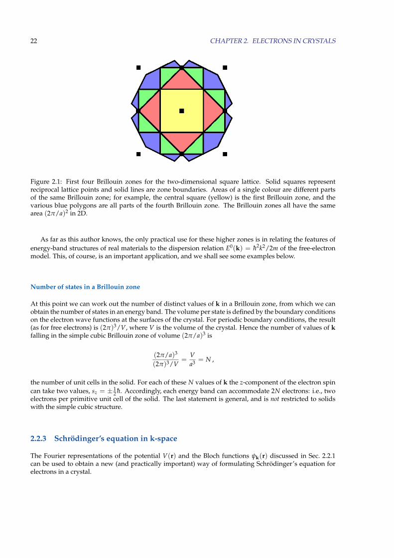
Figure 2.1: First four Brillouin zones for the two-dimensional square lattice. Solid squares representreciprocal lattice points and solid lines are zone boundaries. Areas of a single colour are different partsof the same Brillouin zone; for example, the central square (yellow) is the first Brillouin zone, and thevarious blue polygons are all parts of the fourth Brillouin zone. The Brillouin zones all have the samearea (2π/a)2 in 2D.
As far as this author knows, the only practical use for these higher zones is in relating the features ofenergy-band structures of real materials to the dispersion relation E0(k) = h2k2/2m of the free-electronmodel. This, of course, is an important application, and we shall see some examples below.
Number of states in a Brillouin zone
At this point we can work out the number of distinct values of k in a Brillouin zone, from which we canobtain the number of states in an energy band. The volume per state is defined by the boundary conditionson the electron wave functions at the surfaces of the crystal. For periodic boundary conditions, the result(as for free electrons) is (2π)3/V, where V is the volume of the crystal. Hence the number of values of kfalling in the simple cubic Brillouin zone of volume (2π/a)3 is
(2π/a)3
(2π)3/V=
Va3 = N ,
the number of unit cells in the solid. For each of these N values of k the z-component of the electron spincan take two values, sz = ± 1
2 h. Accordingly, each energy band can accommodate 2N electrons: i.e., twoelectrons per primitive unit cell of the solid. The last statement is general, and is not restricted to solidswith the simple cubic structure.
2.2.3 Schrodinger’s equation in k-space
The Fourier representations of the potential V(r) and the Bloch functions ψk(r) discussed in Sec. 2.2.1can be used to obtain a new (and practically important) way of formulating Schrodinger’s equation forelectrons in a crystal.
2.2. ELECTRONS IN A PERIODIC POTENTIAL 23
We substitute the Fourier expansions (2.6) and (2.9) into the Schrodinger equation (2.2), giving
Eψk(r) = −h2
2m∇2ψk(r) + V(r)ψk(r)
= ∑G
h2
2m(k + G)2 Fk+G ei(k+G)·r + V(r)ψk(r)
≡∑G
E0(k + G) Fk+G ei(k+G)·r + ∑G′
VG′ eiG′ ·r ×∑
KFk+K ei(k+K)·r , (2.10)
where we have written E0(k + G) for the free-electron kinetic energy expression h2(k + G)2/2m. Wewould like to find the equations satisfied by the coefficients Fk+G. The tricky term is the one involvingthe product of V with ψk. To help us to pick out the term in exp[i(k + G) · r] from the product we haverenamed the summation variables G′ and K. This makes it a little easier to show that
∑G′
VG′ eiG′ ·r ×∑
KFk+K ei(k+K)·r = ∑
KFk+K ∑
G′VG′ e
i(k+K+G′)·r
= ∑K
Fk+K ∑G
VG−K ei(k+G)·r , where G = G′ + K
= ∑G
ei(k+G)·r ∑K
VG−K Fk+K ; (2.11)
a change of summation variable has been made in the second line and the order of summation is reversedin going from the second to the third line.3 After inserting (2.11) into (2.10), it is easy to read off thecoefficients of exp[i(k + G) · r] on each side of (2.10). We find
E Fk+G = E0(k + G) Fk+G + ∑K
VG−K Fk+K (2.12)
as the equation satisfied by the coefficients Fk+G : it is fully equivalent to the original Schrodinger equa-tion (2.2). For want of a better name, we call (2.12) Schrodinger’s equation in k-space.
2.2.4 Weak periodic potential: Nearly-free electrons
In the case of a weak periodic potential V(r), we anticipate that the wave functions ψk(r) will be approx-imately free-electron-like,
ψk(r) = eik·r + [small corrections proportional to V],
and that E(k) ' E0(k) ≡ h2k2/2m. We can verify that this guess is consistent with (2.12) for many (butnot all) values of k. For if Fk+G � Fk for G 6= 0 and E ' E0(k), only one term in the sum on theright-hand side of (2.12) needs to be kept (the term with K = 0), and we get
Fk+G '1
E0(k)− E0(k + G)VG Fk for G 6= 0 ;
this is indeed small, provided |VG| � |E0(k)− E0(k + G)|. But it is not hard to see that this approxima-tion for Fk+G will not always be valid, even for small V; it certainly fails when
E0(k) = E0(k + G), i.e., when |k| = |k + G| for some G.
The last condition states that k is equidistant from the points 0 and −G in reciprocal space; that is, k liesanywhere on the zone boundary bisecting the reciprocal lattice vector −G. In this case, we can expect Fkand Fk+G to be of similar magnitude.
3The method here is slightly different from that used in the lecture. Whichever method is used, all we are really doing isestablishing a convolution theorem for the Fourier transforms of periodic functions: the sum over K in (2.11) [and in (2.12)] has theform of a convolution.
24 CHAPTER 2. ELECTRONS IN CRYSTALS
There is another, more physical way of understanding this last result. An electron initially in the free-electron state exp[ik · r] will be strongly scattered by the crystal potential V(r) into a state exp[ik′ · r],provided k′ = k + G, where G is a reciprocal lattice vector: this is just the diffraction condition for wavesin a crystal, which we derived for elastic scattering of X-rays in Chapter 1. For a real (as opposed to virtual)scattering process, energy is conserved, so that E0(k) = E0(k + G), which implies (as above) that k lieson a zone boundary. Hence, if k lies on a zone boundary, the electron wave function must consist (at thevery least) of a term exp[ik · r] for the initial state and a term exp[i(k + G) · r] for the scattered wave.
Dispersion relation E(k) near a zone boundary
As discussed above, near a zone boundary we must consider a wave function consisting of at least twoterms,
ψk(r) ' Fk eik·r + Fk+G ei(k+G)·r .
If no other terms are significant, the equations (2.12) reduce to two equations for the two unknown coef-ficients,
E Fk = E0(k) Fk + V−G Fk+G and E Fk+G = E0(k + G) Fk+G + VG Fk .
To simplify the equations slightly, we have set V0 = 0. This amounts to choosing the arbitrary additiveconstant in the potential energy in such a way that the average of V(r), taken over a unit cell, is zero.4
The two equations for Fk and Fk+G have the form of a 2× 2 matrix eigenvalue problem(E0(k) V−G
VG E0(k + G)
) [Fk
Fk+G
]= E
[Fk
Fk+G
].
The eigenvalue problem can be solved in the usual way, giving
E = 12 [E
0(k) + E0(k + G)]±{ 1
4 [E0(k)− E0(k + G)]2 + |VG|2
}1/2, (2.13)
where we have used V−G = VG∗, which was noted following (2.6).
Many band-structure calculations for real solids follow an approach similar to the one wehave used here. The calculations are extended to include a large (but finite) number of planewaves, so that an M×M matrix eigenvalue problem must be solved for the coefficients Fk+Gand the energy bands. Large matrix eigenvalue problems are a standard topic in numericalanalysis, and C/Fortran subroutine libraries are available to solve them. Similar routines arealso available in Matlab and Mathematica.
Exercise 2.3:
Do the necessary algebra to obtain the result (2.13) for the energy of an electron near a zoneboundary.
The dispersion relation (2.13) simplifies in two special cases. If |VG| � 12 |E0(k)− E0(k + G)|, the two
solutions areE ' E0(k) and E ' E0(k + G) ;
as we should expect, the effect of the crystal potential is negligible if we are far away from the zoneboundary. The other special case is when k lies exactly on the zone boundary, so that E0(k) = E0(k + G).In this case,
E = 12 [E
0(k) + E0(k + G)]± |VG| for k on the zone boundary; (2.14)
the degeneracy E0(k) = E0(k + G) on the zone boundary has been split by the crystal potential: theamount of the splitting is 2|VG|.
4See (2.6), which gives V0 =∫
V(r) d3r/vcell. This expression is the average of V(r), taken over a unit cell.
2.2. ELECTRONS IN A PERIODIC POTENTIAL 25
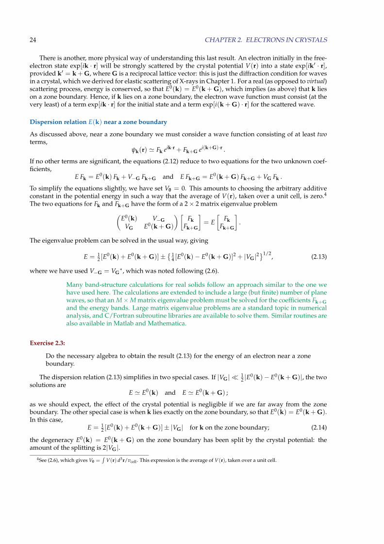
Figure 2.2: Nearly-free electron bands in one dimension, for an electron in the real potential V(x) =2V1 cos(2πx/a), with V1 > 0. The free-electron dispersion relation is indicated by a solid curve; thedotted lines are the bands, as modified by the crystal potential. At the zone boundary, kx = ±π/a, thegap between the first and second bands is 2|V1|; note that for the given potential, the Fourier coeffcientsV1 = V−1 are real and positive, so we could equally well write 2V1 for the gap (as in the figure).
In the second-year course PHYS20252 and in J. Pearson’s notes available online, an alternative methodis given for deriving this energy splitting between the nearly-free electron bands; the argument uses thesymmetry of the electron wave function and simple first-order perturbation theory. This is an excellentapproach, which isn’t superseded by the method given above, but the equation (2.13) contains additionalinformation on the shape of the nearly-free electron energy bands. Nearly-free electron bands are sketchedin Figure 2.2, for the one-dimensional case.
Equation (2.14) is often misunderstood. It does not show that two energy bands are always completelyseparated in energy—even though this happens to be true for an electron in a one-dimensional periodicpotential. In higher dimensions, and if |VG| is not too large, electrons in different bands can have the sameenergy, provided they have different wave vectors. We shall see an important example of this in Sec. 2.2.6, butfirst we remind ourselves of the band-theory account of the difference between metals and insulators.
2.2.5 Metals and insulators
Having argued that a weak crystal potential can lead to energy gaps between bands, we can now formu-late the difference between metals and insulators.
In the ground state of the electron gas in a solid, the electrons occupy the states of lowest energy ofthe lowest-lying bands, consistent, as usual, with the exclusion principle: no more than two electrons(sz = ± 1
2 h) for each value of the wave vector. As we have see already seen, each band can accommodateup to 2N electrons, where N is the number of primitive unit cells in the solid. Therefore, if there is an oddnumber of electrons in the unit cell, at least one band will be only partly filled with electrons: the Fermienergy falls within this band. When an electric field is applied to the solid, the electrons redistributeamong the states near EF to form a current-carrying state at very little cost in energy. The material isconsequently metallic.
If, however, the lowest-lying energy bands are completely full of electrons—this requires an even num-ber of electrons per primitive unit cell—the electrons cannot be redistributed to form a current-carryingstate without exciting them from a filled band across an energy gap to one of the higher, empty bands.This costs a lot of energy, and cannot occur for moderate field strengths: the material is an insulator.
We reach the important conclusions that an insulator, such as diamond, must have an even number ofelectrons per primitive unit cell, and that materials with an odd number, such as sodium, are necessarilymetals.
26 CHAPTER 2. ELECTRONS IN CRYSTALS
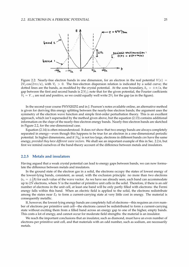
Figure 2.3: Distinction between metals (left) and insulators (right) in the band picture. At T = 0, thebands of an insulator are either all full or all empty, whereas a metal has at least one partly-occupiedband. The electrical properties of a metal are dominated by the electrons at the Fermi energy, EF, whichhave unoccupied states of neighbouring energy that they can transfer to under the action of an appliedelectric field.
Exercise 2.4:
Check these conclusions against the periodic table of the elements, so far as you can.
The converse statements are not necessarily true: for example, the divalent elements zinc and mag-nesium are both metals. In all such cases, although there are enough electrons to fill a whole number ofbands, two or more bands are found to overlap in energy, so that the Fermi energy lies in more than onepartly-filled band. We shall investigate the details of this in the next section, but for the time being wenote that there are three distinct possibilities for the densities of electron states with respect to energy,taking these to be representative of a monovalent metal, a divalent metal, and an insulator. These pos-sibilities are illustrated in Figure 2.3. In the figure, g(E) is the number of electron states per unit energyinterval; this was calculated in detail for free electrons in the second-year course. In this course our onlyexplicit use of g(E) will be, as here, in sketches indicating the presence or absence of energy levels in agiven range of energy.
2.2.6 Band overlap in a nearly-free-electron divalent metal
We consider the case of a simple-cubic divalent metal with one atom per primitive unit cell of side a.5
Diagrams illustrating the occupied states are shown in Figure 2.4 The free-electron Fermi sphere contains2N electrons, so it has the same volume as the first Brillouin zone, which is a cube of side 2π/a. Partsof the Fermi sphere protrude from the faces of the cube. The states “just outside” the Brillouin zonebelong to a different band from those just inside. We can see this by plotting the energy as a function ofkx. It resembles the free-electron result for one dimension, with a gap 2V1 in the dispersion relation6 atkx = π/a.
5The real divalent elements magnesium and zinc both have a close-packed hexagonal structure, and strontium and calcium areface-centered cubic. Similar arguments can be used for these more complex structures.
6Actually, this gap is 2|V100|, since the zone face bisects the reciprocal lattice vector (100), but we simplify the notation here.
2.2. ELECTRONS IN A PERIODIC POTENTIAL 27
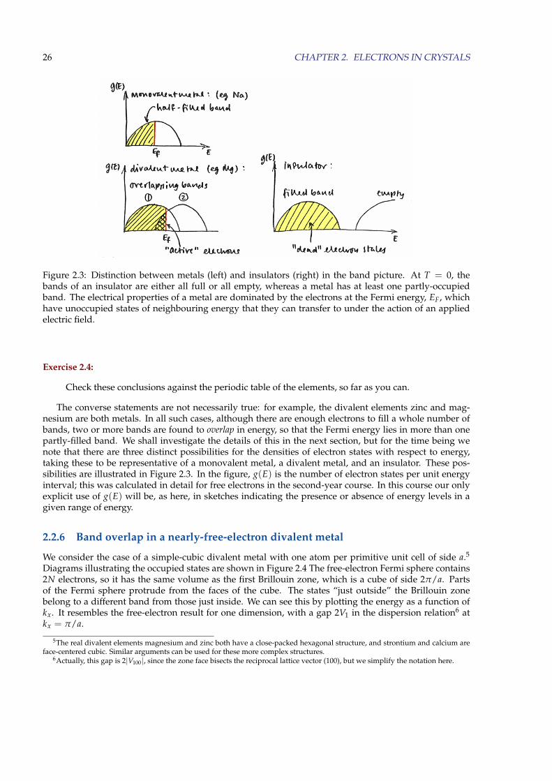
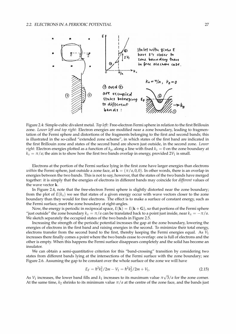
Figure 2.4: Simple-cubic divalent metal. Top left: Free-electron Fermi sphere in relation to the first Brillouinzone. Lower left and top right: Electron energies are modified near a zone boundary, leading to fragmen-tation of the Fermi sphere and distortions of the fragments belonging to the first and second bands; thisis illustrated in the so-called “extended zone scheme”, in which states of the first band are indicated inthe first Brillouin zone and states of the second band are shown just outside, in the second zone. Lowerright: Electron energies plotted as a function of ky, along a line with fixed kz = 0 on the zone boundary atkx = π/a; the aim is to show how the first two bands overlap in energy, provided 2V1 is small.
Electrons at the portion of the Fermi surface lying in the first zone have larger energies than electronswithin the Fermi sphere, just outside a zone face, at k = (π/a, 0, 0). In other words, there is an overlap inenergies between the two bands. This is not to say, however, that the states of the two bands have mergedtogether: it is simply that the energies of electrons in different bands may coincide for different values ofthe wave vector k.
In Figure 2.4, note that the free-electron Fermi sphere is slightly distorted near the zone boundary;from the plot of E(kx) we see that states of a given energy occur with wave vectors closer to the zoneboundary than they would for free electrons. The effect is to make a surface of constant energy, such asthe Fermi surface, meet the zone boundary at right-angles.
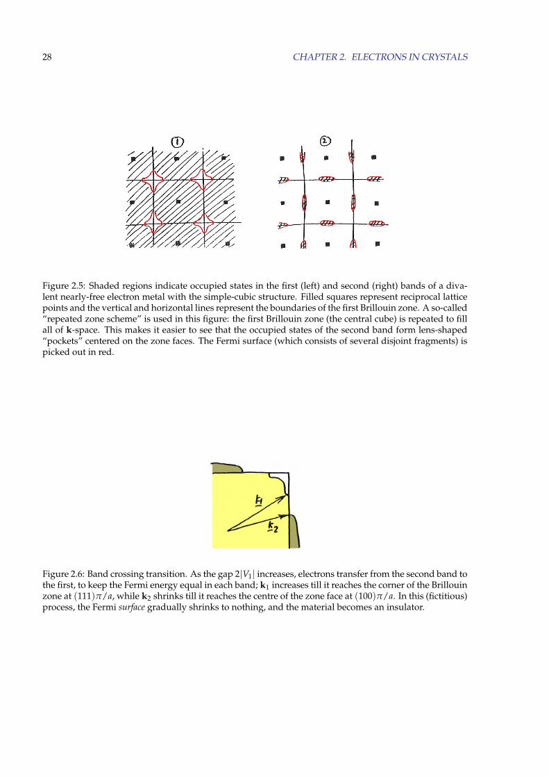
Now, the energy is periodic in reciprocal space, E(k) = E(k + G), so that portions of the Fermi sphere“just outside” the zone boundary kx = π/a can be translated back to a point just inside, near kx = −π/a.We sketch separately the occupied states of the two bands in Figure 2.5.
Increasing the strength of the periodic potential increases the gap at the zone boundary, lowering theenergies of electrons in the first band and raising energies in the second. To minimize their total energy,electrons transfer from the second band to the first, thereby keeping the Fermi energies equal. As V1increases there finally comes a point where the two bands cease to overlap: one is full of electrons and theother is empty. When this happens the Fermi surface disappears completely and the solid has become aninsulator.
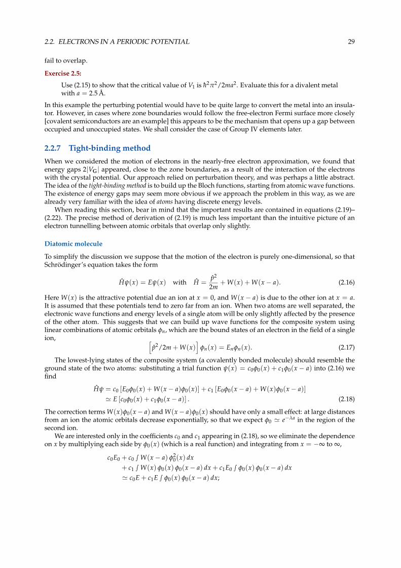
We can obtain a semi-quantitative criterion for this “band-crossing” transition by considering twostates from different bands lying at the intersections of the Fermi surface with the zone boundary; seeFigure 2.6. Assuming the gap to be constant over the whole surface of the zone we will have
EF = h2k21/2m−V1 = h2k2
2/2m + V1. (2.15)
As V1 increases, the lower band fills and k1 increases to its maximum value π√
3/a for the zone corner.At the same time, k2 shrinks to its minimum value π/a at the centre of the zone face, and the bands just
28 CHAPTER 2. ELECTRONS IN CRYSTALS
Figure 2.5: Shaded regions indicate occupied states in the first (left) and second (right) bands of a diva-lent nearly-free electron metal with the simple-cubic structure. Filled squares represent reciprocal latticepoints and the vertical and horizontal lines represent the boundaries of the first Brillouin zone. A so-called“repeated zone scheme” is used in this figure: the first Brillouin zone (the central cube) is repeated to fillall of k-space. This makes it easier to see that the occupied states of the second band form lens-shaped“pockets” centered on the zone faces. The Fermi surface (which consists of several disjoint fragments) ispicked out in red.
Figure 2.6: Band crossing transition. As the gap 2|V1| increases, electrons transfer from the second band tothe first, to keep the Fermi energy equal in each band; k1 increases till it reaches the corner of the Brillouinzone at (111)π/a, while k2 shrinks till it reaches the centre of the zone face at (100)π/a. In this (fictitious)process, the Fermi surface gradually shrinks to nothing, and the material becomes an insulator.
2.2. ELECTRONS IN A PERIODIC POTENTIAL 29
fail to overlap.
Exercise 2.5:
Use (2.15) to show that the critical value of V1 is h2π2/2ma2. Evaluate this for a divalent metalwith a = 2.5 A.
In this example the perturbing potential would have to be quite large to convert the metal into an insula-tor. However, in cases where zone boundaries would follow the free-electron Fermi surface more closely[covalent semiconductors are an example] this appears to be the mechanism that opens up a gap betweenoccupied and unoccupied states. We shall consider the case of Group IV elements later.
2.2.7 Tight-binding method
When we considered the motion of electrons in the nearly-free electron approximation, we found thatenergy gaps 2|VG| appeared, close to the zone boundaries, as a result of the interaction of the electronswith the crystal potential. Our approach relied on perturbation theory, and was perhaps a little abstract.The idea of the tight-binding method is to build up the Bloch functions, starting from atomic wave functions.The existence of energy gaps may seem more obvious if we approach the problem in this way, as we arealready very familiar with the idea of atoms having discrete energy levels.
When reading this section, bear in mind that the important results are contained in equations (2.19)–(2.22). The precise method of derivation of (2.19) is much less important than the intuitive picture of anelectron tunnelling between atomic orbitals that overlap only slightly.
Diatomic molecule
To simplify the discussion we suppose that the motion of the electron is purely one-dimensional, so thatSchrodinger’s equation takes the form
Hψ(x) = Eψ(x) with H =p2
2m+ W(x) + W(x− a). (2.16)
Here W(x) is the attractive potential due an ion at x = 0, and W(x− a) is due to the other ion at x = a.It is assumed that these potentials tend to zero far from an ion. When two atoms are well separated, theelectronic wave functions and energy levels of a single atom will be only slightly affected by the presenceof the other atom. This suggests that we can build up wave functions for the composite system usinglinear combinations of atomic orbitals φn, which are the bound states of an electron in the field of a singleion, [
p2/2m + W(x)]
φn(x) = Enφn(x). (2.17)
The lowest-lying states of the composite system (a covalently bonded molecule) should resemble theground state of the two atoms: substituting a trial function ψ(x) = c0φ0(x) + c1φ0(x − a) into (2.16) wefind
Hψ = c0 [E0φ0(x) + W(x− a)φ0(x)] + c1 [E0φ0(x− a) + W(x)φ0(x− a)]' E [c0φ0(x) + c1φ0(x− a)] . (2.18)
The correction terms W(x)φ0(x− a) and W(x− a)φ0(x) should have only a small effect: at large distancesfrom an ion the atomic orbitals decrease exponentially, so that we expect φ0 ' e−λa in the region of thesecond ion.
We are interested only in the coefficients c0 and c1 appearing in (2.18), so we eliminate the dependenceon x by multiplying each side by φ0(x) (which is a real function) and integrating from x = −∞ to ∞,
c0E0 + c0 ∫ W(x− a) φ20(x) dx
+ c1 ∫ W(x) φ0(x) φ0(x− a) dx + c1E0 ∫ φ0(x) φ0(x− a) dx' c0E + c1E ∫ φ0(x) φ0(x− a) dx;
30 CHAPTER 2. ELECTRONS IN CRYSTALS
where we have used the normalization condition∫
φ20(x) dx = 1. The remaining integrals that involve
products φ0(x) φ0(x − a) all contain the exponential factor e−λa; whereas the integral of W(x − a) φ20(x)
contains two such factors and will be neglected here. The last terms on each side cancel to the same order,because the difference E− E0 is exponentially small.
Carrying out the same procedure after multiplying (2.18) by φ0(x− a) and integrating we obtain twoequations for the unknown coefficients and the energy,
Ec0 ' E0c0 − Bc1 and Ec1 ' E0c1 − Bc0, (2.19)
where
−B =∞∫−∞
W(x) φ0(x) φ0(x− a) dx.
Note that the integral is negative because the two factors φ0 have the same sign and W(x) is attractive.The equations (2.19) can be interpreted intuitively, as a form of Schrodinger’s equation. They say that inthe absence of tunnelling (B = 0) an electron stays on one atom and has energy E0. But if B 6= 0, theelectron can tunnel between atoms, an effect contained in the “hopping terms” −Bc1 and −Bc0.
The solutions of (2.19) are
E = E0 ∓ B for c1 = ±c0 respectively,
so that the ground- and first excited-state solutions of (2.16) are the symmetric and antisymmetric wavefunctions ψs,a = [φ0(x)± φ0(x− a)]/
√2 .
Exercise 2.6:
Check that you can prove the last results.
The atomic energy level E0 for the two atoms has been split into two levels separated by an amount2B which decreases rapidly with increasing separation of the atoms; B is sometimes called the covalentenergy, as it determines the binding energy of the molecule.
Polar molecule
The same picture can be used for a polar (or heteropolar) molecule, in which the constituent atoms X andY (lithium and hydrogen, say) are different. The only change to Schrodinger’s equation (2.19) is to theatomic energy level E0 which must be replaced by values EX , EY appropriate to the two atoms,
EcX = EXcX − BcY and EcY = EYcY − BcX ,
where EY < EX refer respectively to the anion and the cation. Solving the last pair of equations for Egives
E = 12 (EX + EY)±
[14 (EX − EY)
2 + B2]1/2
,
so that in the polar molecule the splitting of the bonding and antibonding energy levels is greater than inthe purely covalent case considered before.
Exercise 2.7:
Verify the last result, and by calculating the coefficients cX , cY show that in the bonding state anelectron is more likely to be found on the anion. [Probabilities are proportional to the squaresof the coefficients.]
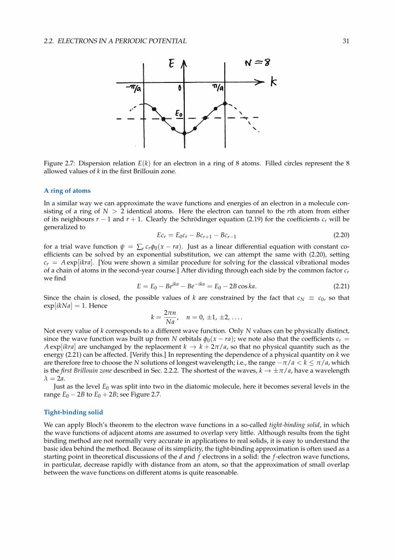
2.2. ELECTRONS IN A PERIODIC POTENTIAL 31
Figure 2.7: Dispersion relation E(k) for an electron in a ring of 8 atoms. Filled circles represent the 8allowed values of k in the first Brillouin zone.
A ring of atoms
In a similar way we can approximate the wave functions and energies of an electron in a molecule con-sisting of a ring of N > 2 identical atoms. Here the electron can tunnel to the rth atom from eitherof its neighbours r − 1 and r + 1. Clearly the Schrodinger equation (2.19) for the coefficients cr will begeneralized to
Ecr = E0cr − Bcr+1 − Bcr−1 (2.20)
for a trial wave function ψ = ∑r crφ0(x − ra). Just as a linear differential equation with constant co-efficients can be solved by an exponential substitution, we can attempt the same with (2.20), settingcr = A exp[ikra]. [You were shown a similar procedure for solving for the classical vibrational modesof a chain of atoms in the second-year course.] After dividing through each side by the common factor crwe find
E = E0 − Beika − Be−ika = E0 − 2B cos ka. (2.21)
Since the chain is closed, the possible values of k are constrained by the fact that cN ≡ c0, so thatexp[ikNa] = 1. Hence
k =2πnNa
, n = 0, ±1, ±2, . . . .
Not every value of k corresponds to a different wave function. Only N values can be physically distinct,since the wave function was built up from N orbitals φ0(x − ra); we note also that the coefficients cr =A exp[ikra] are unchanged by the replacement k → k + 2π/a, so that no physical quantity such as theenergy (2.21) can be affected. [Verify this.] In representing the dependence of a physical quantity on k weare therefore free to choose the N solutions of longest wavelength; i.e., the range−π/a < k ≤ π/a, whichis the first Brillouin zone described in Sec. 2.2.2. The shortest of the waves, k → ±π/a, have a wavelengthλ = 2a.
Just as the level E0 was split into two in the diatomic molecule, here it becomes several levels in therange E0 − 2B to E0 + 2B; see Figure 2.7.
Tight-binding solid
We can apply Bloch’s theorem to the electron wave functions in a so-called tight-binding solid, in whichthe wave functions of adjacent atoms are assumed to overlap very little. Although results from the tightbinding method are not normally very accurate in applications to real solids, it is easy to understand thebasic idea behind the method. Because of its simplicity, the tight-binding approximation is often used as astarting point in theoretical discussions of the d and f electrons in a solid: the f -electron wave functions,in particular, decrease rapidly with distance from an atom, so that the approximation of small overlapbetween the wave functions on different atoms is quite reasonable.
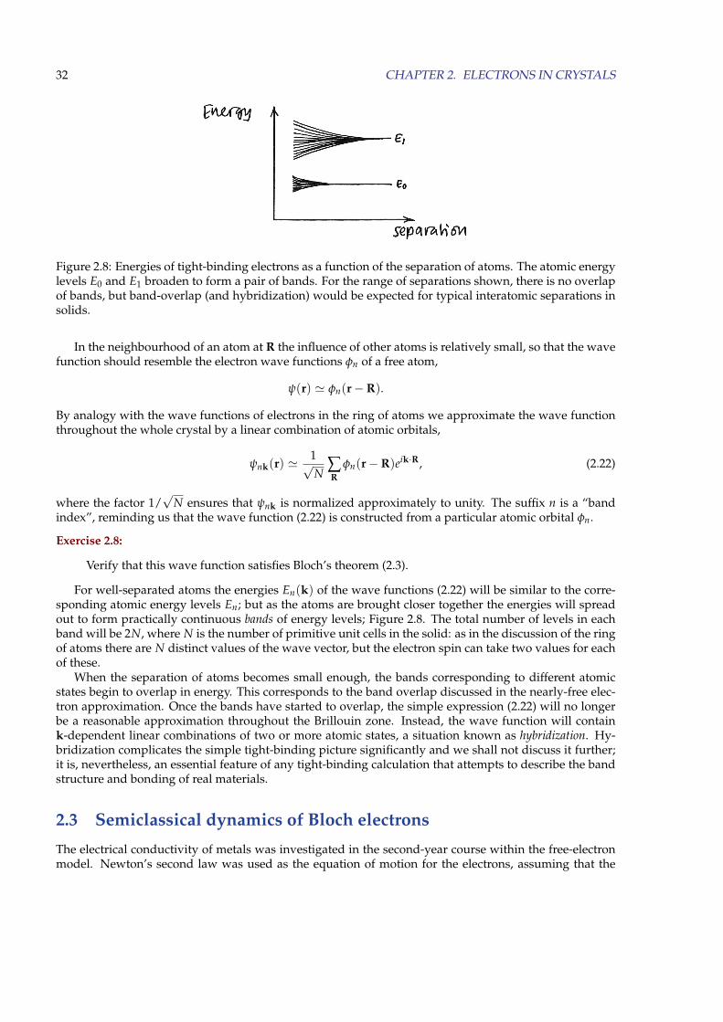
32 CHAPTER 2. ELECTRONS IN CRYSTALS
Figure 2.8: Energies of tight-binding electrons as a function of the separation of atoms. The atomic energylevels E0 and E1 broaden to form a pair of bands. For the range of separations shown, there is no overlapof bands, but band-overlap (and hybridization) would be expected for typical interatomic separations insolids.
In the neighbourhood of an atom at R the influence of other atoms is relatively small, so that the wavefunction should resemble the electron wave functions φn of a free atom,
ψ(r) ' φn(r− R).
By analogy with the wave functions of electrons in the ring of atoms we approximate the wave functionthroughout the whole crystal by a linear combination of atomic orbitals,
ψnk(r) '1√N
∑R
φn(r− R)eik·R, (2.22)
where the factor 1/√
N ensures that ψnk is normalized approximately to unity. The suffix n is a “bandindex”, reminding us that the wave function (2.22) is constructed from a particular atomic orbital φn.
Exercise 2.8:
Verify that this wave function satisfies Bloch’s theorem (2.3).
For well-separated atoms the energies En(k) of the wave functions (2.22) will be similar to the corre-sponding atomic energy levels En; but as the atoms are brought closer together the energies will spreadout to form practically continuous bands of energy levels; Figure 2.8. The total number of levels in eachband will be 2N, where N is the number of primitive unit cells in the solid: as in the discussion of the ringof atoms there are N distinct values of the wave vector, but the electron spin can take two values for eachof these.
When the separation of atoms becomes small enough, the bands corresponding to different atomicstates begin to overlap in energy. This corresponds to the band overlap discussed in the nearly-free elec-tron approximation. Once the bands have started to overlap, the simple expression (2.22) will no longerbe a reasonable approximation throughout the Brillouin zone. Instead, the wave function will containk-dependent linear combinations of two or more atomic states, a situation known as hybridization. Hy-bridization complicates the simple tight-binding picture significantly and we shall not discuss it further;it is, nevertheless, an essential feature of any tight-binding calculation that attempts to describe the bandstructure and bonding of real materials.
2.3 Semiclassical dynamics of Bloch electrons
The electrical conductivity of metals was investigated in the second-year course within the free-electronmodel. Newton’s second law was used as the equation of motion for the electrons, assuming that the
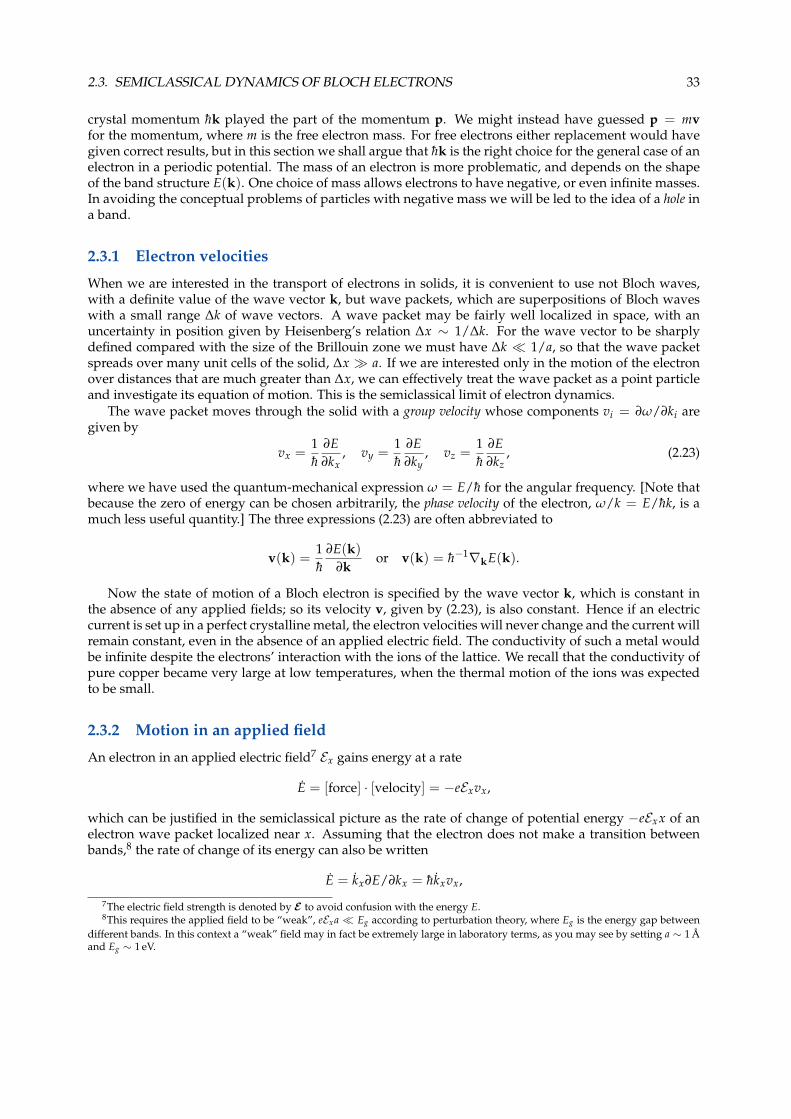
2.3. SEMICLASSICAL DYNAMICS OF BLOCH ELECTRONS 33
crystal momentum hk played the part of the momentum p. We might instead have guessed p = mvfor the momentum, where m is the free electron mass. For free electrons either replacement would havegiven correct results, but in this section we shall argue that hk is the right choice for the general case of anelectron in a periodic potential. The mass of an electron is more problematic, and depends on the shapeof the band structure E(k). One choice of mass allows electrons to have negative, or even infinite masses.In avoiding the conceptual problems of particles with negative mass we will be led to the idea of a hole ina band.
2.3.1 Electron velocities
When we are interested in the transport of electrons in solids, it is convenient to use not Bloch waves,with a definite value of the wave vector k, but wave packets, which are superpositions of Bloch waveswith a small range ∆k of wave vectors. A wave packet may be fairly well localized in space, with anuncertainty in position given by Heisenberg’s relation ∆x ∼ 1/∆k. For the wave vector to be sharplydefined compared with the size of the Brillouin zone we must have ∆k � 1/a, so that the wave packetspreads over many unit cells of the solid, ∆x � a. If we are interested only in the motion of the electronover distances that are much greater than ∆x, we can effectively treat the wave packet as a point particleand investigate its equation of motion. This is the semiclassical limit of electron dynamics.
The wave packet moves through the solid with a group velocity whose components vi = ∂ω/∂ki aregiven by
vx =1h
∂E∂kx
, vy =1h
∂E∂ky
, vz =1h
∂E∂kz
, (2.23)
where we have used the quantum-mechanical expression ω = E/h for the angular frequency. [Note thatbecause the zero of energy can be chosen arbitrarily, the phase velocity of the electron, ω/k = E/hk, is amuch less useful quantity.] The three expressions (2.23) are often abbreviated to
v(k) =1h
∂E(k)∂k
or v(k) = h−1∇kE(k).
Now the state of motion of a Bloch electron is specified by the wave vector k, which is constant inthe absence of any applied fields; so its velocity v, given by (2.23), is also constant. Hence if an electriccurrent is set up in a perfect crystalline metal, the electron velocities will never change and the current willremain constant, even in the absence of an applied electric field. The conductivity of such a metal wouldbe infinite despite the electrons’ interaction with the ions of the lattice. We recall that the conductivity ofpure copper became very large at low temperatures, when the thermal motion of the ions was expectedto be small.
2.3.2 Motion in an applied field
An electron in an applied electric field7 Ex gains energy at a rate
E = [force] · [velocity] = −eExvx,
which can be justified in the semiclassical picture as the rate of change of potential energy −eExx of anelectron wave packet localized near x. Assuming that the electron does not make a transition betweenbands,8 the rate of change of its energy can also be written
E = kx∂E/∂kx = hkxvx,
7The electric field strength is denoted by E to avoid confusion with the energy E.8This requires the applied field to be “weak”, eExa � Eg according to perturbation theory, where Eg is the energy gap between
different bands. In this context a “weak” field may in fact be extremely large in laboratory terms, as you may see by setting a ∼ 1 Aand Eg ∼ 1 eV.
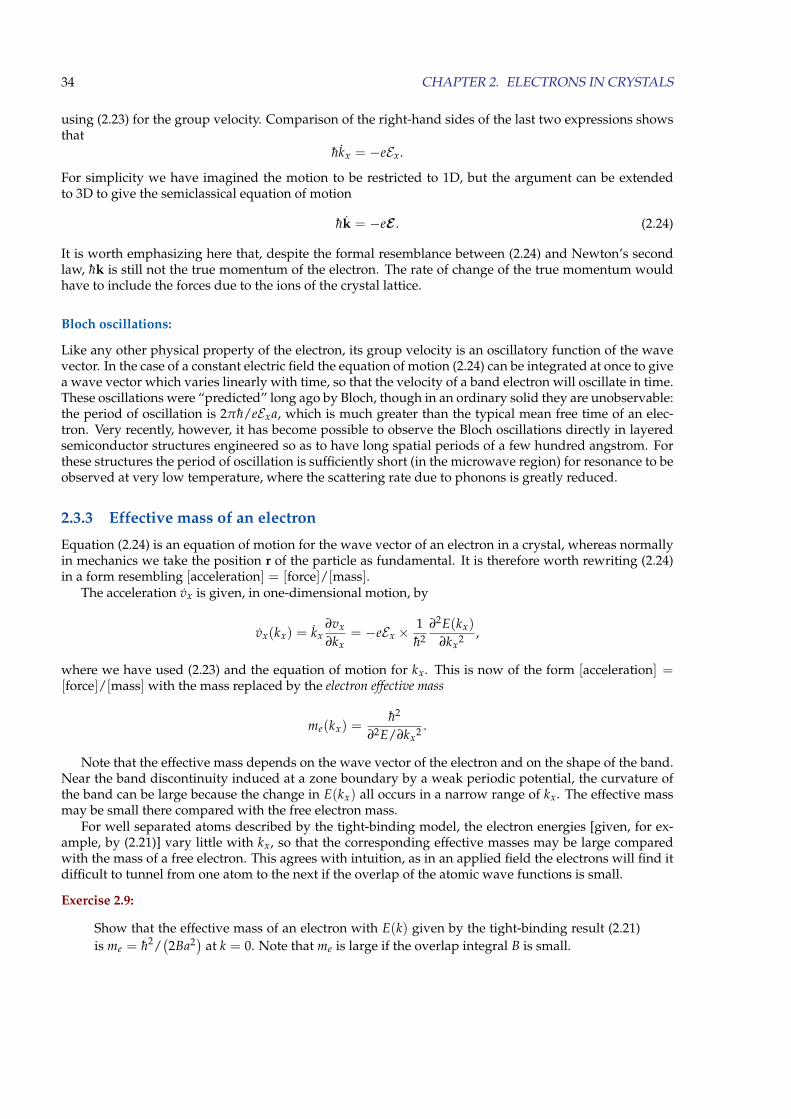
34 CHAPTER 2. ELECTRONS IN CRYSTALS
using (2.23) for the group velocity. Comparison of the right-hand sides of the last two expressions showsthat
hkx = −eEx.
For simplicity we have imagined the motion to be restricted to 1D, but the argument can be extendedto 3D to give the semiclassical equation of motion
hk = −eE . (2.24)
It is worth emphasizing here that, despite the formal resemblance between (2.24) and Newton’s secondlaw, hk is still not the true momentum of the electron. The rate of change of the true momentum wouldhave to include the forces due to the ions of the crystal lattice.
Bloch oscillations:
Like any other physical property of the electron, its group velocity is an oscillatory function of the wavevector. In the case of a constant electric field the equation of motion (2.24) can be integrated at once to givea wave vector which varies linearly with time, so that the velocity of a band electron will oscillate in time.These oscillations were “predicted” long ago by Bloch, though in an ordinary solid they are unobservable:the period of oscillation is 2πh/eExa, which is much greater than the typical mean free time of an elec-tron. Very recently, however, it has become possible to observe the Bloch oscillations directly in layeredsemiconductor structures engineered so as to have long spatial periods of a few hundred angstrom. Forthese structures the period of oscillation is sufficiently short (in the microwave region) for resonance to beobserved at very low temperature, where the scattering rate due to phonons is greatly reduced.
2.3.3 Effective mass of an electron
Equation (2.24) is an equation of motion for the wave vector of an electron in a crystal, whereas normallyin mechanics we take the position r of the particle as fundamental. It is therefore worth rewriting (2.24)in a form resembling [acceleration] = [force]/[mass].
The acceleration vx is given, in one-dimensional motion, by
vx(kx) = kx∂vx
∂kx= −eEx ×
1h2
∂2E(kx)
∂kx2 ,
where we have used (2.23) and the equation of motion for kx. This is now of the form [acceleration] =[force]/[mass] with the mass replaced by the electron effective mass
me(kx) =h2
∂2E/∂kx2 .
Note that the effective mass depends on the wave vector of the electron and on the shape of the band.Near the band discontinuity induced at a zone boundary by a weak periodic potential, the curvature ofthe band can be large because the change in E(kx) all occurs in a narrow range of kx. The effective massmay be small there compared with the free electron mass.
For well separated atoms described by the tight-binding model, the electron energies [given, for ex-ample, by (2.21)] vary little with kx, so that the corresponding effective masses may be large comparedwith the mass of a free electron. This agrees with intuition, as in an applied field the electrons will find itdifficult to tunnel from one atom to the next if the overlap of the atomic wave functions is small.
Exercise 2.9:
Show that the effective mass of an electron with E(k) given by the tight-binding result (2.21)is me = h2/
(2Ba2) at k = 0. Note that me is large if the overlap integral B is small.
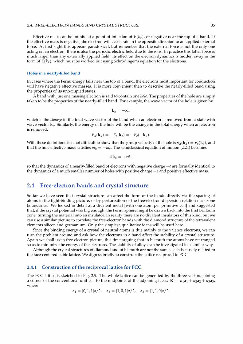
2.4. FREE-ELECTRON BANDS AND CRYSTAL STRUCTURE 35
Effective mass can be infinite at a point of inflexion of E(kx), or negative near the top of a band. Ifthe effective mass is negative, the electron will accelerate in the opposite direction to an applied externalforce. At first sight this appears paradoxical, but remember that the external force is not the only oneacting on an electron: there is also the periodic electric field due to the ions. In practice this latter force ismuch larger than any externally applied field. Its effect on the electron dynamics is hidden away in theform of E(kx), which must be worked out using Schrodinger’s equation for the electrons.
Holes in a nearly-filled band
In cases where the Fermi energy falls near the top of a band, the electrons most important for conductionwill have negative effective masses. It is more convenient then to describe the nearly-filled band usingthe properties of its unoccupied states.
A band with just one missing electron is said to contain one hole. The properties of the hole are simplytaken to be the properties of the nearly-filled band. For example, the wave vector of the hole is given by
kh = −ke,
which is the change in the total wave vector of the band when an electron is removed from a state withwave vector ke. Similarly, the energy of the hole will be the change in the total energy when an electronis removed,
Eh(kh) = −Ee(ke) = −Ee(−kh).
With these definitions it is not difficult to show that the group velocity of the hole is vh(kh) = ve(ke), andthat the hole effective mass satisfies mh = −me. The semiclassical equation of motion (2.24) becomes
hkh = +eE ,
so that the dynamics of a nearly-filled band of electrons with negative charge −e are formally identical tothe dynamics of a much smaller number of holes with positive charge +e and positive effective mass.
2.4 Free-electron bands and crystal structure
So far we have seen that crystal structure can affect the form of the bands directly via the spacing ofatoms in the tight-binding picture, or by perturbation of the free-electron dispersion relation near zoneboundaries. We looked in detail at a divalent metal [with one atom per primitive cell] and suggestedthat, if the crystal potential was big enough, the Fermi sphere might be drawn back into the first Brillouinzone, turning the material into an insulator. In reality there are no divalent insulators of this kind, but wecan use a similar picture to correlate the free-electron bands with the diamond structure of the tetravalentelements silicon and germanium. Only the simplest, qualitative ideas will be used here.
Since the binding energy of a crystal of neutral atoms is due mainly to the valence electrons, we canturn the problem around and ask how the electrons in a band affect the stability of a crystal structure.Again we shall use a free-electron picture, this time arguing that in bismuth the atoms have rearrangedso as to minimize the energy of the electrons. The stability of alloys can be investigated in a similar way.
Although the crystal structures of diamond and of bismuth are not the same, each is closely related tothe face-centered cubic lattice. We digress briefly to construct the lattice reciprocal to FCC.
2.4.1 Construction of the reciprocal lattice for FCC
The FCC lattice is sketched in Fig. 2.9. The whole lattice can be generated by the three vectors joininga corner of the conventional unit cell to the midpoints of the adjoining faces: R = n1a1 + n2a2 + n3a3,where
a1 = [0, 1, 1]a/2, a2 = [1, 0, 1]a/2, a3 = [1, 1, 0]a/2.
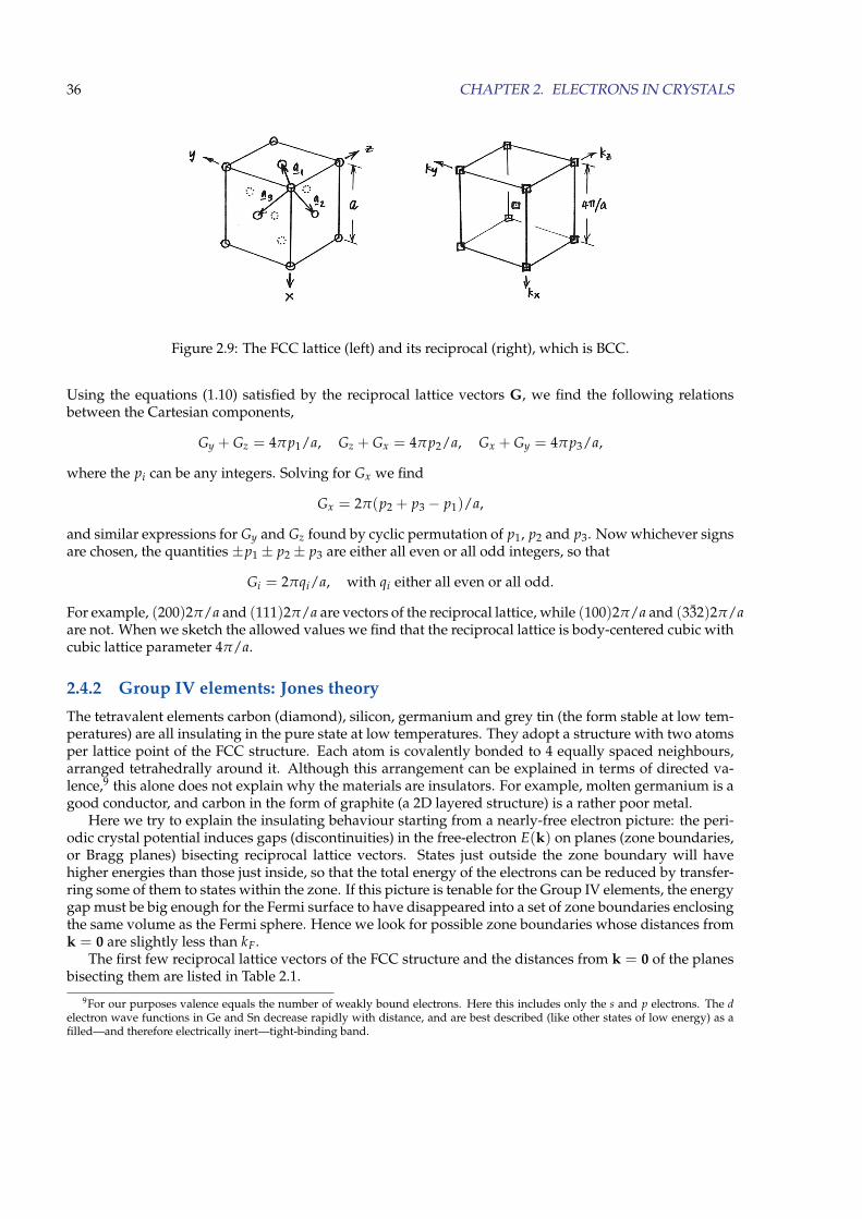
36 CHAPTER 2. ELECTRONS IN CRYSTALS
Figure 2.9: The FCC lattice (left) and its reciprocal (right), which is BCC.
Using the equations (1.10) satisfied by the reciprocal lattice vectors G, we find the following relationsbetween the Cartesian components,
Gy + Gz = 4πp1/a, Gz + Gx = 4πp2/a, Gx + Gy = 4πp3/a,
where the pi can be any integers. Solving for Gx we find
Gx = 2π(p2 + p3 − p1)/a,
and similar expressions for Gy and Gz found by cyclic permutation of p1, p2 and p3. Now whichever signsare chosen, the quantities ±p1 ± p2 ± p3 are either all even or all odd integers, so that
Gi = 2πqi/a, with qi either all even or all odd.
For example, (200)2π/a and (111)2π/a are vectors of the reciprocal lattice, while (100)2π/a and (332)2π/aare not. When we sketch the allowed values we find that the reciprocal lattice is body-centered cubic withcubic lattice parameter 4π/a.
2.4.2 Group IV elements: Jones theory
The tetravalent elements carbon (diamond), silicon, germanium and grey tin (the form stable at low tem-peratures) are all insulating in the pure state at low temperatures. They adopt a structure with two atomsper lattice point of the FCC structure. Each atom is covalently bonded to 4 equally spaced neighbours,arranged tetrahedrally around it. Although this arrangement can be explained in terms of directed va-lence,9 this alone does not explain why the materials are insulators. For example, molten germanium is agood conductor, and carbon in the form of graphite (a 2D layered structure) is a rather poor metal.
Here we try to explain the insulating behaviour starting from a nearly-free electron picture: the peri-odic crystal potential induces gaps (discontinuities) in the free-electron E(k) on planes (zone boundaries,or Bragg planes) bisecting reciprocal lattice vectors. States just outside the zone boundary will havehigher energies than those just inside, so that the total energy of the electrons can be reduced by transfer-ring some of them to states within the zone. If this picture is tenable for the Group IV elements, the energygap must be big enough for the Fermi surface to have disappeared into a set of zone boundaries enclosingthe same volume as the Fermi sphere. Hence we look for possible zone boundaries whose distances fromk = 0 are slightly less than kF.
The first few reciprocal lattice vectors of the FCC structure and the distances from k = 0 of the planesbisecting them are listed in Table 2.1.
9For our purposes valence equals the number of weakly bound electrons. Here this includes only the s and p electrons. The delectron wave functions in Ge and Sn decrease rapidly with distance, and are best described (like other states of low energy) as afilled—and therefore electrically inert—tight-binding band.
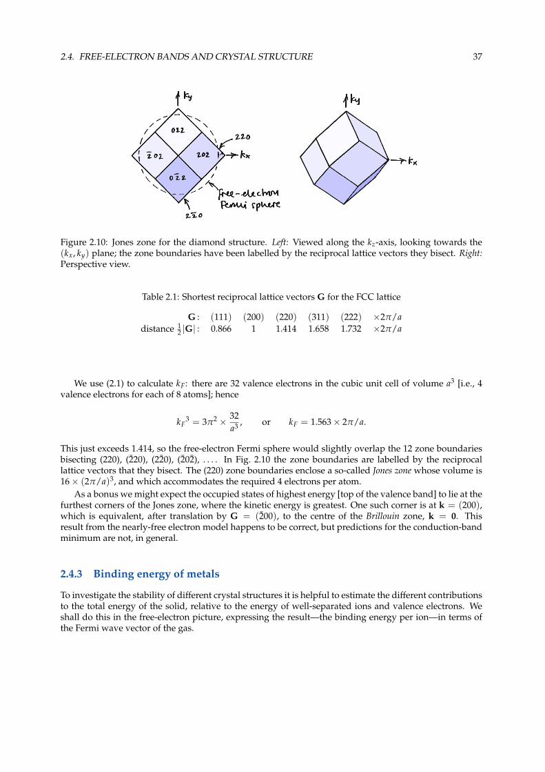
2.4. FREE-ELECTRON BANDS AND CRYSTAL STRUCTURE 37
Figure 2.10: Jones zone for the diamond structure. Left: Viewed along the kz-axis, looking towards the(kx, ky) plane; the zone boundaries have been labelled by the reciprocal lattice vectors they bisect. Right:Perspective view.
Table 2.1: Shortest reciprocal lattice vectors G for the FCC lattice
G : (111) (200) (220) (311) (222) ×2π/adistance 1
2 |G| : 0.866 1 1.414 1.658 1.732 ×2π/a
We use (2.1) to calculate kF: there are 32 valence electrons in the cubic unit cell of volume a3 [i.e., 4valence electrons for each of 8 atoms]; hence
kF3 = 3π2 × 32
a3 , or kF = 1.563× 2π/a.
This just exceeds 1.414, so the free-electron Fermi sphere would slightly overlap the 12 zone boundariesbisecting (220), (220), (220), (202), . . . . In Fig. 2.10 the zone boundaries are labelled by the reciprocallattice vectors that they bisect. The (220) zone boundaries enclose a so-called Jones zone whose volume is16× (2π/a)3, and which accommodates the required 4 electrons per atom.
As a bonus we might expect the occupied states of highest energy [top of the valence band] to lie at thefurthest corners of the Jones zone, where the kinetic energy is greatest. One such corner is at k = (200),which is equivalent, after translation by G = (200), to the centre of the Brillouin zone, k = 0. Thisresult from the nearly-free electron model happens to be correct, but predictions for the conduction-bandminimum are not, in general.
2.4.3 Binding energy of metals
To investigate the stability of different crystal structures it is helpful to estimate the different contributionsto the total energy of the solid, relative to the energy of well-separated ions and valence electrons. Weshall do this in the free-electron picture, expressing the result—the binding energy per ion—in terms ofthe Fermi wave vector of the gas.
38 CHAPTER 2. ELECTRONS IN CRYSTALS
Kinetic energy:
The free electron kinetic energy has been worked out in PHYS20252 and again in PHYS30151. Here wesimply quote the result
Ekin = 35 NeEF = 3
5 Ne · h2kF2/2m.
Since each of the Ni ions has contributed Z electrons to the gas, the total number of electrons is Ne = NiZ,giving
Ekin/Ni =3
10 Zh2kF2/m (2.25)
as the electron kinetic energy per ion.
Electrostatic energy:
We make a rather drastic approximation that the ions can be regarded as point charges. The calculationof the electrostatic energy of point ions in a uniform electron gas is fairly involved, and analogous to thecalculation of the electrostatic energy of ionic solids. We shall not go into details, but will quote the resultin the conventional form
ECoul/Ni = −12
e2
4πε0
Z2α
r0, (2.26)
where r0 is the radius of a so-called atomic sphere, which encloses the point ion and Z electrons. Thedimensionless constant α is characteristic of the particular crystal structure, like the Madelung constantfor ionic solids. The radius of the atomic sphere is related (see Problem 2.4) to kF by
r0 = (9πZ/4)1/3/kF. (2.27)
Most simple metals adopt one of the three structures FCC, BCC or HCP (hexagonal close-packed), forwhich α = 1.79; the atoms are close together, giving the lowest (i.e., most negative) electrostatic energy.The more open simple-cubic structure (α = 1.76) and diamond structure (α = 1.67) are not favoured; thelatter is stabilized by the kind of “zone effect” that is discussed below for the pentavalent semi-metals.
Total electronic energy:
Using (2.25), (2.26) and (2.27) we find the total energy per ion to be
Etot/Ni =3Zh2kF
2
10 m− e2
4πε0
αZ2kF
(18πZ)1/3 .
The value of kF that minimizes the total energy can be found by differentiating the last expression; thefinal results are
k∗F =53
αZ2/3
(18π)1/3mh2
e2
4πε0and E∗tot/Ni = −
3Zh2k∗F2
10 m
for the optimum Fermi wave vector k∗F and the corresponding minimum energy E∗tot.
Z k∗F [A−1] −E∗tot/Ni [eV]
sodium 1 1.47 (0.91) 4.9 (6.3)magnesium 2 2.33 (1.37) 24.8 (24.4)aluminium 3 3.05 (1.75) 63.8 (56.3)
Predictions for the binding energy are not too far from the experimental values (given in brackets),but the Fermi wave vectors are much less accurately estimated. Note also that our results depend only onvalence, so they cannot represent the variation among elements of the same group [column of the periodic
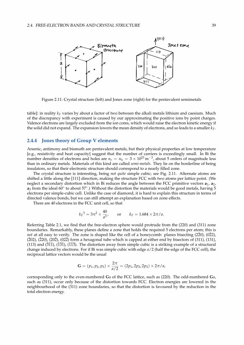
2.4. FREE-ELECTRON BANDS AND CRYSTAL STRUCTURE 39
Figure 2.11: Crystal structure (left) and Jones zone (right) for the pentavalent semimetals
table]: in reality kF varies by about a factor of two between the alkali metals lithium and caesium. Muchof the discrepancy with experiment is caused by our approximating the positive ions by point charges.Valence electrons are largely excluded from the ion cores, which would raise the electron kinetic energy ifthe solid did not expand. The expansion lowers the mean density of electrons, and so leads to a smaller kF.
2.4.4 Jones theory of Group V elements
Arsenic, antimony and bismuth are pentavalent metals, but their physical properties at low temperature[e.g., resistivity and heat capacity] suggest that the number of carriers is exceedingly small. In Bi thenumber densities of electrons and holes are ne = nh = 3× 10²³ m−3, about 5 orders of magnitude lessthan in ordinary metals. Materials of this kind are called semi-metals. They lie on the borderline of beinginsulators, so that their electronic structure should correspond to a nearly filled zone.
The crystal structure is interesting, being not quite simple cubic; see Fig. 2.11. Alternate atoms areshifted a little along the [111] direction, making the structure FCC with two atoms per lattice point. (Weneglect a secondary distortion which in Bi reduces the angle between the FCC primitive vectors a1, a2,a3 from the ideal 60◦ to about 57◦.) Without the distortion the materials would be good metals, having 5electrons per simple-cubic cell. Unlike the case of diamond, it is hard to explain this structure in terms ofdirected valence bonds, but we can still attempt an explanation based on zone effects.
There are 40 electrons in the FCC unit cell, so that
kF3 = 3π2 × 40
a3 , or kF = 1.684× 2π/a.
Referring Table 2.1, we find that the free-electron sphere would protrude from the (220) and (311) zoneboundaries. Remarkably, these planes define a zone that holds the required 5 electrons per atom; this isnot at all easy to verify. The zone is shaped like the cell of a honeycomb: planes bisecting (220), (022),(202), (220), (202), (022) form a hexagonal tube which is capped at either end by bisectors of (311), (131),(113) and (311), (131), (113). The distortion away from simple cubic is a striking example of a structuralchange induced by electrons. For if Bi was simple cubic with edge a/2 (half the edge of the FCC cell), thereciprocal lattice vectors would be the usual
G = (p1, p2, p3)×2π
a/2= (2p1, 2p2, 2p3)× 2π/a,
corresponding only to the even-numbered Gs of the FCC lattice, such as (220). The odd-numbered Gs,such as (311), occur only because of the distortion towards FCC. Electron energies are lowered in theneighbourhood of the (311) zone boundaries, so that the distortion is favoured by the reduction in thetotal electron energy.
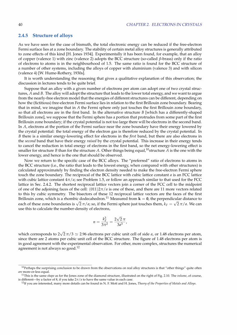
40 CHAPTER 2. ELECTRONS IN CRYSTALS
2.4.5 Structure of alloys
As we have seen for the case of bismuth, the total electronic energy can be reduced if the free-electronFermi surface lies at a zone boundary. The stability of certain metal alloy structures is generally attributedto zone effects of this kind [H. Jones 1934]. Experimentally it has been found, for example, that an alloyof copper (valence 1) with zinc (valence 2) adopts the BCC structure (so-called β-brass) only if the ratioof electrons to atoms is in the neighbourhood of 1.5. The same ratio is found for the BCC structure ofa number of other systems, including the alloys of copper with aluminium (valence 3) and with silicon(valence 4) [W. Hume-Rothery, 1930s].
It is worth understanding the reasoning that gives a qualitative explanation of this observation; thediscussion in lectures tends to be quite brief.
Suppose that an alloy with a given number of electrons per atom can adopt one of two crystal struc-tures, A and B. The alloy will adopt the structure that leads to the lower total energy, and we want to arguefrom the nearly-free electron model that the energies of different structures can be different, depending onhow the (fictitious) free-electron Fermi surface lies in relation to the first Brillouin zone boundary. Bearingthat in mind, we imagine that in A the Fermi sphere only just touches the first Brillouin zone boundary,so that all electrons are in the first band. In the alternative structure B [which has a differently-shapedBrillouin zone], we suppose that the Fermi sphere has a portion that protrudes from some part of the firstBrillouin zone boundary; if the crystal potential is not too large there will be electrons in the second band.In A, electrons at the portion of the Fermi surface near the zone boundary have their energy lowered bythe crystal potential: the total energy of the electron gas is therefore reduced by the crystal potential. InB there is a similar energy-lowering effect for electrons in the first band, but there are also electrons inthe second band that have their energy raised by the crystal potential. This increase in their energy tendsto cancel the reduction in total energy of electrons in the first band, so the net energy-lowering effect issmaller for structure B than for the structure A. Other things being equal,10structure A is the one with thelower energy, and hence is the one that should be observed.
Now we return to the specific case of the BCC alloys. The “preferred” ratio of electrons to atoms inthe BCC structure (i.e., the ratio that leads to the lowest energy, when compared with other structures) iscalculated approximately by finding the electron density needed to make the free-electron Fermi spheretouch the zone boundary. The reciprocal of the BCC lattice with cubic lattice constant a is an FCC latticewith cubic lattice constant 4π/a; see Problem 1.5, or follow an approach similar to that used for the FCClattice in Sec. 2.4.2. The shortest reciprocal lattice vectors join a corner of the FCC cell to the midpointof one of the adjoining faces of the cell: (011)2π/a is one of these, and there are 11 more vectors relatedto this by cubic symmetry. The bisectors of these 12 reciprocal lattice vectors are the faces of the firstBrillouin zone, which is a rhombic dodecahedron.11 Measured from k = 0, the perpendicular distance toeach of these zone boundaries is
√2 π/a; so, if the Fermi sphere just touches them, kF =
√2 π/a. We can
use this to calculate the number-density of electrons,
n =k3
F3π2 =
2√
2 π
3a3 ,
which corresponds to 2√
2 π/3 ' 2.96 electrons per cubic unit cell of side a, or 1.48 electrons per atom,since there are 2 atoms per cubic unit cell of the BCC structure. The figure of 1.48 electrons per atom isin good agreement with the experimental observation. For other, more complex, structures the numericalagreement is not always so good.12
10Perhaps the surprising conclusion to be drawn from the observations on real alloy structures is that “other things” quite oftenare more-or-less equal.
11This is the same shape as for the Jones zone of the diamond structure, illustrated on the right of Fig. 2.10. The volume, of course,is different—by a factor of 8, if you take 2π/a to have the same value in each case.
12If you are interested, many more details can be found in N. F. Mott and H. Jones, Theory of the Properties of Metals and Alloys.

2.5. CYCLOTRON RESONANCE 41
Figure 2.12: Cyclotron resonance in silicon at 24 GHz and 4 K; after Dresselhaus et al., 1955.
2.5 Cyclotron resonance
In a uniform magnetic field B a classical free electron moves in a circle (or a helix) with angular fre-quency ωc. If the radius of the orbit is a, the speed will be ωca and the Lorentz force of magnitude eωcaBwill give rise to the centripetal acceleration. Hence13
m0ω2c a = eωcaB, or ωc = eB/m0.
When an electromagnetic (e.g., microwave) field of fixed frequency is applied, energy will be absorbedby the electron if its orbital frequency matches that of the applied field. By varying the uniform magneticfield and monitoring the microwave absorption it would be possible to calculate m0 from the position ofthe peak in the absorption plotted as a function of B.
The basic principle is the same for cyclotron resonance measurements of effective masses of carriersin semiconductors. In general, a cyclotron effective mass mc can be defined from the resonance frequencyand the applied field, mc = eB/ωc.
To obtain sharp resonance peaks the carriers must complete at least a few orbits before being scattered.Pure samples and low temperatures (about 4 kelvin) must therefore be used to reduce scattering by im-purities and phonons. But unlike free space, crystals are not isotropic, so that orbits are not necessarilycircular and the analysis is usually more complicated. Extra information is needed, such as the positionsof the resonances as the direction of the magnetic field is varied. An example of this kind of analysis isgiven in Problem 2.5, but you should read the next two sections before attempting it.
2.5.1 Effective mass tensor
First we need to investigate the form of the electron dispersion relation near a minimum of the conductionband. Although it is not easy to calculate E(k) for particular semiconductors, some general propertiesdepend only on the symmetry of the solid, and we consider these below. Similar considerations apply toholes near the top of the valence band.
To simplify things we assume that the atomic arrangement in the semiconductor is simple cubic. Thefirst Brillouin zone is then a cube of side 2π/a, where a is the lattice constant. We only need to considerone such cube because the energy is periodic in k: E(k) = E(k+G), where G is a reciprocal lattice vector.
The precise form of E(k) depends on the position of the minimum in the zone; see Fig. 2.13. Supposethat it occurs at the zone centre, k = 0. We expand the energy in a power series with respect to k aboutthis point. The first non-zero terms are
E(k) = E(0) +h2
2me
(k2
x + k2y + k2
z
)+ higher powers of k, (2.28)
13From now on we make clear when the free-electron mass (previously denoted by m) is being used by giving it a subscript zero,m0 ≡ m = 9.1× 10⁻³¹ kg.
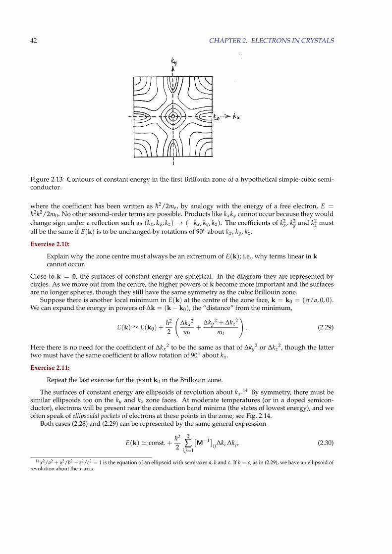
42 CHAPTER 2. ELECTRONS IN CRYSTALS
Figure 2.13: Contours of constant energy in the first Brillouin zone of a hypothetical simple-cubic semi-conductor.
where the coefficient has been written as h2/2me, by analogy with the energy of a free electron, E =h2k2/2m0. No other second-order terms are possible. Products like kxky cannot occur because they wouldchange sign under a reflection such as (kx, ky, kz) → (−kx, ky, kz). The coefficients of k2
x, k2y and k2
z mustall be the same if E(k) is to be unchanged by rotations of 90◦ about kx, ky, kz.
Exercise 2.10:
Explain why the zone centre must always be an extremum of E(k); i.e., why terms linear in kcannot occur.
Close to k = 0, the surfaces of constant energy are spherical. In the diagram they are represented bycircles. As we move out from the centre, the higher powers of k become more important and the surfacesare no longer spheres, though they still have the same symmetry as the cubic Brillouin zone.
Suppose there is another local minimum in E(k) at the centre of the zone face, k = k0 = (π/a, 0, 0).We can expand the energy in powers of ∆k = (k− k0), the “distance” from the minimum,
E(k) ' E(k0) +h2
2
(∆kx
2
ml+
∆ky2 + ∆kz
2
mt
). (2.29)
Here there is no need for the coefficient of ∆kx2 to be the same as that of ∆ky
2 or ∆kz2, though the latter
two must have the same coefficient to allow rotation of 90◦ about kx.
Exercise 2.11:
Repeat the last exercise for the point k0 in the Brillouin zone.
The surfaces of constant energy are ellipsoids of revolution about kx.14 By symmetry, there must besimilar ellipsoids too on the ky and kz zone faces. At moderate temperatures (or in a doped semicon-ductor), electrons will be present near the conduction band minima (the states of lowest energy), and weoften speak of ellipsoidal pockets of electrons at these points in the zone; see Fig. 2.14.
Both cases (2.28) and (2.29) can be represented by the same general expression
E(k) ' const. +h2
2
3
∑i,j=1
[M−1]
ij∆ki ∆k j, (2.30)
14x2/a2 + y2/b2 + z2/c2 = 1 is the equation of an ellipsoid with semi-axes a, b and c. If b = c, as in (2.29), we have an ellipsoid ofrevolution about the x-axis.
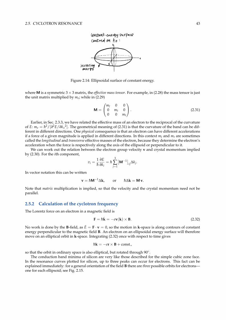
2.5. CYCLOTRON RESONANCE 43
Figure 2.14: Ellipsoidal surface of constant energy.
where M is a symmetric 3× 3 matrix, the effective mass tensor. For example, in (2.28) the mass tensor is justthe unit matrix multiplied by me; while in (2.29)
M =
ml 0 00 mt 00 0 mt
. (2.31)
Earlier, in Sec. 2.3.3, we have related the effective mass of an electron to the reciprocal of the curvatureof E: me = h2/[∂2E/∂kx
2]. The geometrical meaning of (2.31) is that the curvature of the band can be dif-ferent in different directions. One physical consequence is that an electron can have different accelerationsif a force of a given magnitude is applied in different directions. In this context ml and mt are sometimescalled the longitudinal and transverse effective masses of the electron, because they determine the electron’sacceleration when the force is respectively along the axis of the ellipsoid or perpendicular to it.
We can work out the relation between the electron group velocity v and crystal momentum impliedby (2.30). For the ith component,
vi =1h
∂E∂ki
= h3
∑j=1
[M−1]
ij∆k j.
In vector notation this can be written
v = hM−1∆k, or h∆k = M v.
Note that matrix multiplication is implied, so that the velocity and the crystal momentum need not beparallel.
2.5.2 Calculation of the cyclotron frequency
The Lorentz force on an electron in a magnetic field is
F = hk = −ev(k)× B. (2.32)
No work is done by the B-field, as E = F · v = 0, so the motion in k-space is along contours of constantenergy perpendicular to the magnetic field B. An electron on an ellipsoidal energy surface will thereforemove on an elliptical orbit in k-space. Integrating (2.32) once with respect to time gives
hk = −er× B + const.,
so that the orbit in ordinary space is also elliptical, but rotated through 90◦.The conduction band minima of silicon are very like those described for the simple cubic zone face.
In the resonance curves plotted for silicon, up to three peaks can occur for electrons. This fact can beexplained immediately: for a general orientation of the field B there are three possible orbits for electrons—one for each ellipsoid; see Fig. 2.15.
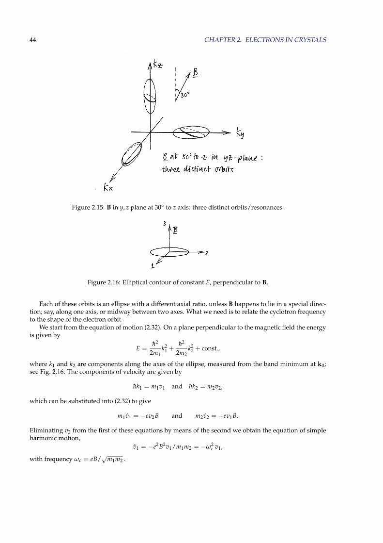
44 CHAPTER 2. ELECTRONS IN CRYSTALS
Figure 2.15: B in y, z plane at 30◦ to z axis: three distinct orbits/resonances.
Figure 2.16: Elliptical contour of constant E, perpendicular to B.
Each of these orbits is an ellipse with a different axial ratio, unless B happens to lie in a special direc-tion; say, along one axis, or midway between two axes. What we need is to relate the cyclotron frequencyto the shape of the electron orbit.
We start from the equation of motion (2.32). On a plane perpendicular to the magnetic field the energyis given by
E =h2
2m1k2
1 +h2
2m2k2
2 + const.,
where k1 and k2 are components along the axes of the ellipse, measured from the band minimum at k0;see Fig. 2.16. The components of velocity are given by
hk1 = m1v1 and hk2 = m2v2,
which can be substituted into (2.32) to give
m1v1 = −ev2B and m2v2 = +ev1B.
Eliminating v2 from the first of these equations by means of the second we obtain the equation of simpleharmonic motion,
v1 = −e2B2v1/m1m2 = −ω2c v1,
with frequency ωc = eB/√
m1m2 .
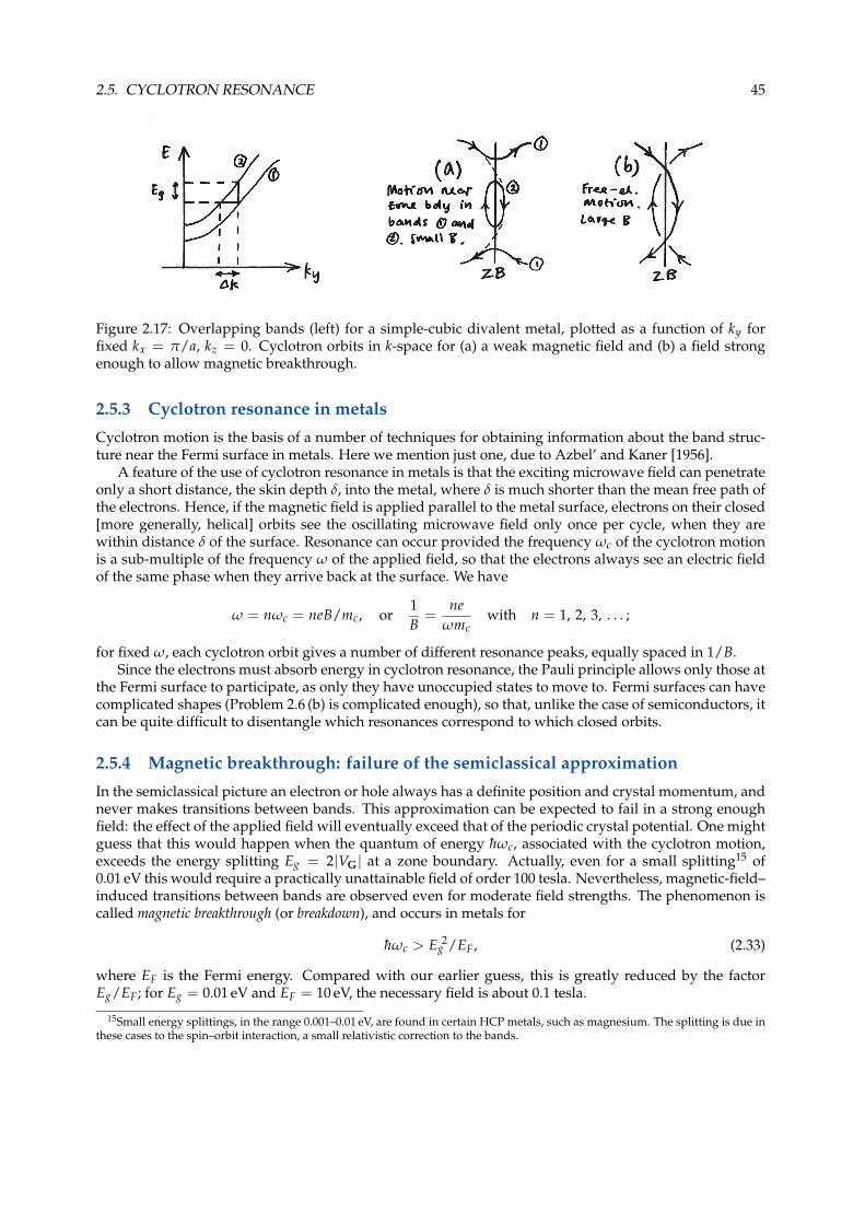
2.5. CYCLOTRON RESONANCE 45
Figure 2.17: Overlapping bands (left) for a simple-cubic divalent metal, plotted as a function of ky forfixed kx = π/a, kz = 0. Cyclotron orbits in k-space for (a) a weak magnetic field and (b) a field strongenough to allow magnetic breakthrough.
2.5.3 Cyclotron resonance in metals
Cyclotron motion is the basis of a number of techniques for obtaining information about the band struc-ture near the Fermi surface in metals. Here we mention just one, due to Azbel’ and Kaner [1956].
A feature of the use of cyclotron resonance in metals is that the exciting microwave field can penetrateonly a short distance, the skin depth δ, into the metal, where δ is much shorter than the mean free path ofthe electrons. Hence, if the magnetic field is applied parallel to the metal surface, electrons on their closed[more generally, helical] orbits see the oscillating microwave field only once per cycle, when they arewithin distance δ of the surface. Resonance can occur provided the frequency ωc of the cyclotron motionis a sub-multiple of the frequency ω of the applied field, so that the electrons always see an electric fieldof the same phase when they arrive back at the surface. We have
ω = nωc = neB/mc, or1B=
neωmc
with n = 1, 2, 3, . . . ;
for fixed ω, each cyclotron orbit gives a number of different resonance peaks, equally spaced in 1/B.Since the electrons must absorb energy in cyclotron resonance, the Pauli principle allows only those at
the Fermi surface to participate, as only they have unoccupied states to move to. Fermi surfaces can havecomplicated shapes (Problem 2.6 (b) is complicated enough), so that, unlike the case of semiconductors, itcan be quite difficult to disentangle which resonances correspond to which closed orbits.
2.5.4 Magnetic breakthrough: failure of the semiclassical approximation
In the semiclassical picture an electron or hole always has a definite position and crystal momentum, andnever makes transitions between bands. This approximation can be expected to fail in a strong enoughfield: the effect of the applied field will eventually exceed that of the periodic crystal potential. One mightguess that this would happen when the quantum of energy hωc, associated with the cyclotron motion,exceeds the energy splitting Eg = 2|VG| at a zone boundary. Actually, even for a small splitting15 of0.01 eV this would require a practically unattainable field of order 100 tesla. Nevertheless, magnetic-field–induced transitions between bands are observed even for moderate field strengths. The phenomenon iscalled magnetic breakthrough (or breakdown), and occurs in metals for
hωc > Eg2/EF, (2.33)
where EF is the Fermi energy. Compared with our earlier guess, this is greatly reduced by the factorEg/EF; for Eg = 0.01 eV and EF = 10 eV, the necessary field is about 0.1 tesla.
15Small energy splittings, in the range 0.001–0.01 eV, are found in certain HCP metals, such as magnesium. The splitting is due inthese cases to the spin–orbit interaction, a small relativistic correction to the bands.
46 CHAPTER 2. ELECTRONS IN CRYSTALS
It is not too hard to understand the criterion (2.33) in a qualitative way, using the uncertainty principleof quantum mechanics. We have found in Sec. 2.5.2 that cyclotron orbits in r-space are geometricallysimilar to the contours of constant energy followed by the carrier in k-space. The orbit is rotated by 90◦
and scaled by a factor depending on the field so that, for example, hky = eBx + const. Hence the usualuncertainty principle ∆kx ∆x > 1 becomes an uncertainty principle relating the two components of thewave vector,
∆kx ∆ky > eB/h.
In the presence of a magnetic field, therefore, the wave vector cannot be defined with a precision greaterthan about ∆kc =
√eB/h .
Now we envisage a case similar to that illustrated on the left of Fig. 2.17: two overlapping nearly-freeelectron bands separated in energy by Eg. As shown in the figure, states of the same energy in the twobands occur at different wave vectors, the separation being ∆k. If ∆k is less than the uncertainty in kit is an over-refinement to say that the electron is in a definite band [case (a) in Fig. 2.17, for small B];instead, we might expect to find cyclotron motion (and resonance spectra) characteristic of free electronsin a magnetic field [case (b), large B]. Quantitatively this requires
∆kc > ∆k =Eg
∂E/∂k.
At the Fermi energy the velocity is vF = h−1∂E/∂k. Using this and the expression for ∆kc in the lastinequality we find
√eB/h > Eg/hvF or eB/h >
(Eg/hvF
)2 ∼ m0Eg2/h2EF.
When making a rough estimate we should not be too worried about being wrong by a factor of 2, so wehave replaced vF
2 by EF/m0 to get the last expression; multiplying each side by h2/m0 finally gives thecriterion (2.33).
Chapter 3
Magnetism
The magnetic properties of matter include its response to an applied magnetic field. Since this is governedlargely by the response of the electrons (effects due to nuclear magnetic moments are at least six orders ofmagnitude smaller) it is useful to study the motion of charged particles in a magnetic field.
3.1 Electrons in a magnetic field
The classical Newtonian description of the motion of charges is easy,
mv = Q(E + v× B) , (3.1)
where E and B are applied electric and magnetic fields and m and Q are the mass and electric chargeof the particle. The problem is how to include the effect of the velocity-dependent Lorentz force in aSchrodinger equation
Hψ(r) = E ψ(r) .
Usually we simply take H to be the classical expression for the energy of the particle and replace the ki-netic energy by the operator p2/2m. But a time-independent magnetic field does no work on the electron(v× B is perpendicular to v) and so has no direct effect on the energy
E =mv2
2+ Qφ(r) , (3.2)
where φ(r) is the scalar potential of the electric field, E = −∇φ . It is worth recalling here that H playsa dual role in quantum mechanics: besides being the energy, it also determines the time development ofthe system via the time-dependent Schrodinger equation. Before we attempt any quantum mechanics wewill show how the energy also determines the time development in classical mechanics.1
3.1.1 Hamiltonians in classical mechanics
A wide range of classical mechanical systems can be described using Hamilton’s equations, which we writedown for the simplest case of one particle:
r =∂H∂p
(3.3)
p = −∂H∂r
. (3.4)
1For this course, the only important result in Sections 3.1.1 and 3.1.2 is Eq. (3.5), the Hamiltonian of a charge in an electromagneticfield. Some students have already met this, but I think it is useful for everyone to have an idea of where this mysterious-lookingresult comes from.
47
48 CHAPTER 3. MAGNETISM
The Hamiltonian energy function H(p, r) introduced here depends on the momentum and position of theparticle; ∂H/∂r is just an alternative notation for ∇H, and ∂H/∂p similarly means the derivative withrespect to components of p.
We verify that a particle in a potential V(r) can be described by (3.3)–(3.4). In this case the Hamiltonianis p2/2m + V(r), and Hamilton’s equations give
r =∂H∂p
= p/m and p = −∂H∂r
= −∇V ;
the first of these simply says that the momentum is mv; the second is Newton’s second law. We can thinkof the complete Hamiltonian as a generalization of the potential, V(r): as with V, the derivative of H withrespect to r gives the rate of change of p; but in addition the derivative with respect to p give the rate ofchange of r. This symmetry in the treatment of position and momentum is one of the attractive featuresof Hamilton’s method.
Not all systems can be described by a Hamiltonian, just as they cannot all be described by a La-grangian; frictional forces, for example, cannot be treated in this way. Nevertheless, if we can write ourequations of motion in the canonical form (3.3)–(3.4) it is generally possible to go over to the quantum caseby replacing p by −ih∇.
3.1.2 Classical Hamiltonian of a charge in a magnetic field
We need to find a Hamiltonian that describes velocity-dependent forces, such as those in (3.1). The energy(3.2), expressed in terms of r and v, does not involve the magnetic field, while H(p, r) (which is alsosupposed to be the energy) must involve B, since this appears in the equation of motion. It seems likely,therefore, that the magnetic field should enter via the dependence of p on v. We write
p = mv + QA ,
where QA is expected to vanish if B = 0, or if the particle has no charge. When this form is substitutedin the left-hand side of (3.4) time derivatives of A appear, in addition to mv. These extra terms (whentransferred to the other side of the equation) are contributions to the force on the electron. If A dependson v this force will depend on acceleration, in contradiction to (3.1); hence we expect A to depend onlyon position. From (3.3) we then find
∂H∂p
= r =(p−QA(r)
)/m ,
which can be integrated with respect to p to obtain
H =(p−QA)2
2m+ V(r) , (3.5)
where V(r) is an (as yet) undetermined function of position.We finally verify that (3.5) leads to the Lorentz force equation when substituted into (3.4). A straight-
forward calculation of the derivatives gives
p = mv + Q(v · ∇)A = −∂H∂r
= −∇V + Q3
∑i=1
(pi −QAi)∇Ai
≡ −∇V + Q3
∑i=1
vi∇Ai ,
3.1. ELECTRONS IN A MAGNETIC FIELD 49
so that, after taking the term Q(v · ∇)A to the other side of the equation,
mv = −∇V + Q3
∑i=1
vi∇Ai −Q(v · ∇)A
= −∇V + Qv× [∇×A]
≡ QE + Qv× B ;
the second line is obtained by inspection of the formula for the vector triple product, P × [R × S] =(P · S)R − (P · R)S = ∑i PiRSi − (P · R)S . The second and third lines show that QE = −∇V andB = ∇×A : we can now identify V/Q = φ with the scalar potential of the electric field and A with themagnetic vector potential.
Note that, because of the modified relation between p and v, the Hamiltonian (3.5) is precisely theanticipated energy function (3.2), but expressed in different variables.
Exercise 3.1:
Extend the treatment to allow for time-varying fields, and hence show that E = −∇φ− ∂A/∂tin general.
3.1.3 No magnetism in classical physics
The result from the last section allows us to calculate the additional magnetic field generated by a systemin an applied magnetic field B. We might expect some such effect: free charges in a magnetic field movein circular (or helical) orbits, and so should behave like little current loops. According to the Biot–Savartlaw, the magnetic field induced at r′ by a charge Q moving with velocity v at r is given by
Bind(r′, r, v) =
µ0
4π
Qv× (r′ − r)|r′ − r|3 .
More generally, the induced magnetic field will be the sum of many such terms, taken over all the elec-trons of the system. In practice we are interested not in the instantaneous value of this sum, which wouldbe a very rapidly fluctuating quantity, but in its value 〈Bind〉 averaged over the motion of the electrons atthermal equilibrium. We might anticipate one of the following three possibilities:
(a) 〈Bind〉 parallel to the applied field, and vanishing as B→ 0. This case is called paramagnetism and isfound in many simple metals, such as sodium, and in salts of the transition metals.
(b) 〈Bind〉 anti-parallel to the applied field, and vanishing for B → 0. This is called diamagnetism andit is found experimentally in rare-gas solids (frozen neon, say), covalently-bonded insulators, semi-metals such as bismuth, and very often in gases of carriers in semiconductors.
(c) 〈Bind〉 parallel to the applied field, but not vanishing for small fields: the material is said to have aspontaneous magnetization, or to be ferromagnetic. The archetypal ferromagnet is iron, but there areother ferromagnetic transition metals and rare-earths, and many alloys.
In fact none of the above occur in classical physics, as we can see by forming the average 〈Bind〉 using theBoltzmann distribution. We have
〈Bind〉 =∫∫
Bind(r′, r, v) exp[−H(p, r)/kBT] d3p d3r/h3∫∫exp[−H(p, r)/kBT] d3p d3r/h3
=
∫∫Bind(r′, r, v) exp
[−( 1
2 mv2 + V(r))/kBT
]d3v d3r∫∫
exp[−( 1
2 mv2 + V(r))/kBT
]d3v d3r
,
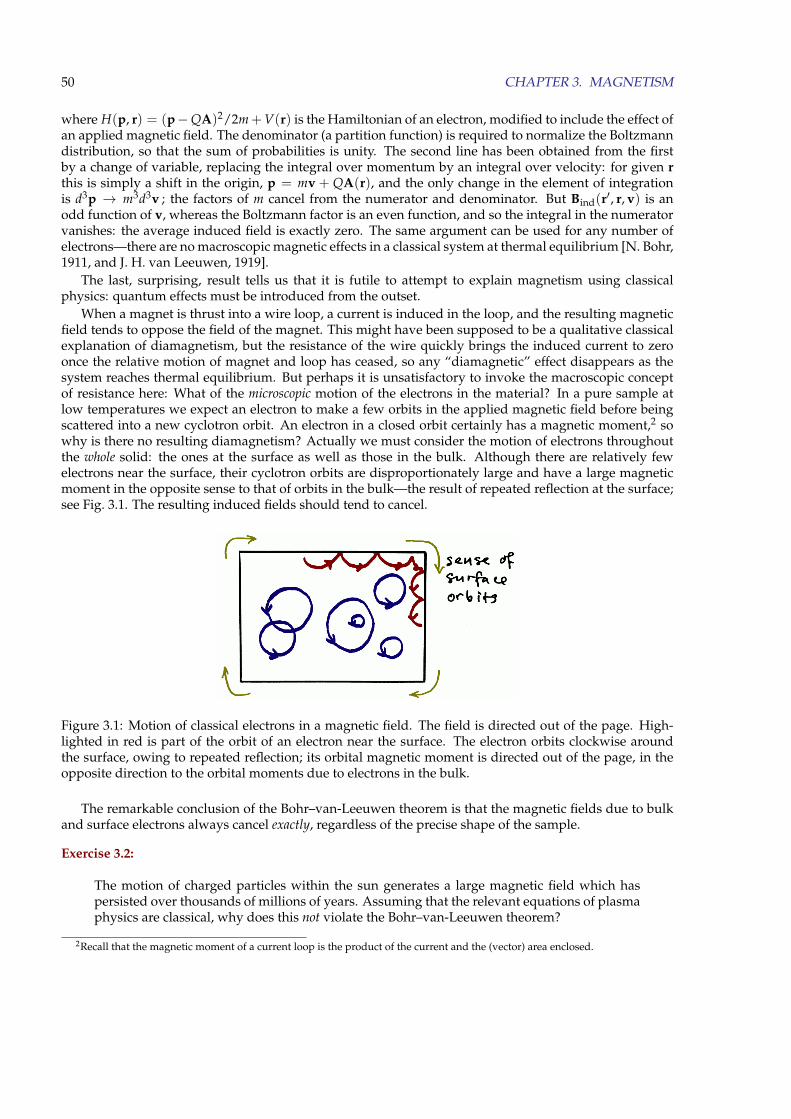
50 CHAPTER 3. MAGNETISM
where H(p, r) = (p−QA)2/2m+V(r) is the Hamiltonian of an electron, modified to include the effect ofan applied magnetic field. The denominator (a partition function) is required to normalize the Boltzmanndistribution, so that the sum of probabilities is unity. The second line has been obtained from the firstby a change of variable, replacing the integral over momentum by an integral over velocity: for given rthis is simply a shift in the origin, p = mv + QA(r), and the only change in the element of integrationis d3p → m3d3v ; the factors of m cancel from the numerator and denominator. But Bind(r′, r, v) is anodd function of v, whereas the Boltzmann factor is an even function, and so the integral in the numeratorvanishes: the average induced field is exactly zero. The same argument can be used for any number ofelectrons—there are no macroscopic magnetic effects in a classical system at thermal equilibrium [N. Bohr,1911, and J. H. van Leeuwen, 1919].
The last, surprising, result tells us that it is futile to attempt to explain magnetism using classicalphysics: quantum effects must be introduced from the outset.
When a magnet is thrust into a wire loop, a current is induced in the loop, and the resulting magneticfield tends to oppose the field of the magnet. This might have been supposed to be a qualitative classicalexplanation of diamagnetism, but the resistance of the wire quickly brings the induced current to zeroonce the relative motion of magnet and loop has ceased, so any “diamagnetic” effect disappears as thesystem reaches thermal equilibrium. But perhaps it is unsatisfactory to invoke the macroscopic conceptof resistance here: What of the microscopic motion of the electrons in the material? In a pure sample atlow temperatures we expect an electron to make a few orbits in the applied magnetic field before beingscattered into a new cyclotron orbit. An electron in a closed orbit certainly has a magnetic moment,2 sowhy is there no resulting diamagnetism? Actually we must consider the motion of electrons throughoutthe whole solid: the ones at the surface as well as those in the bulk. Although there are relatively fewelectrons near the surface, their cyclotron orbits are disproportionately large and have a large magneticmoment in the opposite sense to that of orbits in the bulk—the result of repeated reflection at the surface;see Fig. 3.1. The resulting induced fields should tend to cancel.
Figure 3.1: Motion of classical electrons in a magnetic field. The field is directed out of the page. High-lighted in red is part of the orbit of an electron near the surface. The electron orbits clockwise aroundthe surface, owing to repeated reflection; its orbital magnetic moment is directed out of the page, in theopposite direction to the orbital moments due to electrons in the bulk.
The remarkable conclusion of the Bohr–van-Leeuwen theorem is that the magnetic fields due to bulkand surface electrons always cancel exactly, regardless of the precise shape of the sample.
Exercise 3.2:
The motion of charged particles within the sun generates a large magnetic field which haspersisted over thousands of millions of years. Assuming that the relevant equations of plasmaphysics are classical, why does this not violate the Bohr–van-Leeuwen theorem?
2Recall that the magnetic moment of a current loop is the product of the current and the (vector) area enclosed.
3.2. MAGNETIC QUANTITIES IN THERMODYNAMICS 51
3.1.4 Quantum Hamiltonian of an electron in a magnetic field
There are two contributions to the interaction of an electron with a magnetic field. One of these, the partdue to the electron’s orbital motion, is the quantized version of (3.5),
Horb = (p−QA)2/2me,
where p = −ih∇ is the momentum operator, and Q = −e is the (negative) electronic charge; for simplicitywe have assumed an isotropic effective mass me for the electron, and this need not equal the free-electronmass m0. The second, purely quantum, effect is the intrinsic magnetic moment associated with the elec-tron’s spin s, and this interacts directly with the applied field,
Hspin = −mspin · B, where mspin = −2µB s/h = −µBσ.
Here µB = eh/2m0 is the Bohr magneton, numerically equal to 9.3 × 10⁻²⁴ J T−1, and σ = (σx, σy, σz)are the Pauli spin matrices. At this point all we need to know about the spin matrices is that they haveeigenvalues ±1, so that the energy of a spin in a uniform magnetic field B is ∓µBB.
3.2 Magnetic quantities in thermodynamics
For later use we give some definitions of magnetic quantities, starting at the microscopic level and build-ing up to the relations of macroscopic thermodynamics.
The orbital magnetic moment of a charge Q moving with velocity v can be defined as
morb = 12 Q r× v . (3.6)
This is consistent with Ampere’s definition (footnote 2) because r× δr/2 is the vector area of the trianglespanned by r and δr = v δt, so when averaged over a closed orbit (3.6) gives the required product ofcurrent and area.
Exercise 3.3:
Verify this by forming the time average∫
morb dt/T for a closed orbit of period T. Note thatQ/T is the mean current.
Now consider the change in the Hamiltonian H(p, r) when the externally applied uniform magneticfield B changes by δB. Only the kinetic part of H depends on B, via the vector potential,
δH = δ(p−QA)2/2m = −Q δA · (p−QA)/m ≡ −Q δA · v .
For a uniform field, A can be taken as 12 B× r, so that
δH = − 12 Q δB× r · v = − 1
2 Q r× v · δB = −morb · δB ,
where the cyclic property of the scalar triple product has been used.When averaged over the motion of the charge, δH gives the energy change, and so must equal the
“magnetic work” done on the charge. [Physically, the work is done by the electric field E = −∂A/∂t,induced when the magnetic field is changing; as noted before, the magnetic field itself does no work.]The work done on a body is
δWmag = −M · δB = −M δB ,
where M is its total magnetic moment, i.e., the sum of the moments of all the individual charges; tosimplify the notation in the final expression we have assumed that M, B and δB are all in the samedirection. For a quantum mechanical system at zero temperature the work done must equal the changein the ground-state energy E0(B), so we have
M = −∂E0
∂B.
52 CHAPTER 3. MAGNETISM
The magnetic susceptibility χ of a linear material (as most are at small fields) is defined by M = χH.However, for materials that are only weakly magnetic the field intensity H is very nearly equal to B/µ0, sowe can write
χ ' µ0MB
= µ0∂M∂B
= −µ0∂2E0
∂B2 .
A paramagnetic substance has χ > 0, a diamagnetic one has χ < 0. If M denotes the magnetization, i.e., themagnetic dipole moment per unit volume (M = B/µ0 −H), χ will be dimensionless, but it is also commonpractice to refer M and χ to different quantities of matter, e.g., to one mole or one kilogram, rather thanto one cubic metre of material; for example, if M is referred to one mole, its units will be A m2 mol−1 andthe units of χ will be m3 mol−1.
The variation of the energy with B gives a way of measuring the magnetic moment of a sample. In afield which varies slowly with position x,
[force on sample] = −∂E0
∂x= −∂E0
∂B∂B∂x
= M∂B∂x
.
Exercise 3.4:
Show that a paramagnetic substance tends to be drawn into regions of greater magnetic field,while a diamagnet is expelled.
The expression for the magnetic work is not restricted to zero temperature, so we can find how theserelations are generalized to T 6= 0. From the fundamental theorem of thermodynamics, the change in theenergy of a body in a magnetic field is
dE = dWmag + T dS = −M dB + T dS,
where E and S (the entropy) refer to the same amount of substance as M. Hence in a change at constanttemperature M dB = −dE + T dS = −d(E− TS), or
M = −(
∂F∂B
)T
, (3.7)
where F ≡ E− TS is the Helmholtz free energy of the system. The earlier expressions for χ and for theforce on a body are generalized simply by replacing E0 by F.
3.3 Magnetism of a gas of free electrons
A general calculation of the magnetic properties of a gas of free electrons is difficult. To keep the treatmentsimple, we suppose that the gas is at high temperature or low density. In this limit, the Fermi–Diracdistribution function reduces to the Maxwell–Boltzmann form,
f (Ei) ' exp[(µ− Ei)/kBT],
where µ is the chemical potential of the electrons.3 The Maxwell-Boltzmann limit is appropriate to carriersin a lightly-doped semiconductor, but not (for example) to electrons in a metal.
Leaving aside the application to semiconductors, the reason it is helpful to consider this limit is thatEi, just like the Hamiltonian, can be separated into spin and orbital contributions, Ei = Ei,spin + Ei,orb.When the energy is a sum of terms, the Maxwell–Boltzmann distribution can be written as a product offactors
f (Ei) ∝ e−(Ei,spin+Ei,orb)/kBT = e−Ei,spin/kBT × e−Ei,orb/kBT ;
i.e., the spin and orbital degrees of freedom are statistically independent, and so can be considered sepa-rately. This is what we do in the next two sections.
3However, for the purposes of this course, you can just regard the factor exp[µ/kBT] as a normalization factor, chosen so that thesum of the f (Ei), taken over all states, equals the number of electrons in the system.
3.3. MAGNETISM OF A GAS OF FREE ELECTRONS 53
3.3.1 Pauli spin paramagnetism of an electron gas
Here we calculate the spin magnetic moment of an electron in a low-density electron gas, by using theBoltzmann distribution. The spin contribution to its energy is ±µBB, so the thermal average of the elec-tron’s magnetic moment is
Mspin =µBeµBB/kBT − µBe−µBB/kBT
eµBB/kBT + e−µBB/kBT = µB tanh[µBB/kBT].
For sufficiently large fields (µBB � kBT), the tanh function approaches the value 1; as might have beenexpected, the electron’s magnetic moment aligns with the applied field. Because of the small size of µBwe more usually have the opposite case µBB� kBT, so the tanh can be approximated by the first term ofits Taylor series, tanh x ' x, giving
Mspin ' µ2BB/kBT =
(eh
2m0
)2 BkBT
. (3.8)
The magnetization is in the same direction as the applied field, so the spins are paramagnetic. Note thatthe result is proportional to 1/m2
0, which explains why the contribution from the much more massivenuclear spins can usually be neglected.
3.3.2 Landau orbital diamagnetism of an electron gas
The classical cyclotron motion of electrons in a uniform magnetic field consists of free motion parallel tothe field and circular motion of frequency ωc = eB/me perpendicular to the field. If the field is in the zdirection we might expect the energy levels to have the form
En(kz) =(n + 1
2)hωc + h2k2
z/2me,
where n = 0, 1, 2, . . . , numbers the energy levels of the harmonic motion, called, in this context, the Landaulevels. This guess for the energy levels can be confirmed by straightforward calculation [Problem 3.x,maybe]. A crucial result from the full quantum treatment is that each Landau level is highly degenerate:there are G = eBA/h states corresponding to any given values of n and kz.4 Accordingly the entropy of anelectron with given n and kz is given by Boltzmann’s formula
Sn = kB ln G = kB ln[eBA/h].
The orbital magnetic moment of an electron in the nth Landau level can be found from (3.7)
Mn = −∂En
∂B+ T
∂Sn
∂B= −
(n + 1
2) eh
me+
kBTB
.
It is relatively simple to average this magnetization with respect to the Boltzmann distribution, which isvalid at low density or high temperature: 〈n〉, the mean number of quanta in a harmonic oscillator, isgiven by the Bose distribution, and the remaining terms are independent of the Landau level,
Morb = −(〈n〉+ 1
2) eh
me+
kBTB
= −{
1ehωc/kBT − 1
+12
}ehme
+kBT
B.
The expression in curly brackets is identical to 12 coth[hωc/2kBT], which for small fields (small ωc) can be
expanded in the series coth x ' x−1 + 13 x. The term in the expansion proportional to 1/B is cancelled
exactly by the entropy term kBT/B, and we are left with
Morb ' −13
(eh
2me
)2 BkBT
. (3.9)
The magnetization is in the opposite direction to B, corresponding to diamagnetism.4We might expect the “number of places” we can put a cyclotron orbit to be proportional to the area A. The field dependence is
the result of an uncertainty principle for the position (x0, y0) of the orbit centre: ∆x0 ∆y0 ∼ h/eB.
54 CHAPTER 3. MAGNETISM
3.3.3 Total magnetic response of the electron gas
If we compare the expressions (3.8) and (3.9), we notice that they are of the same form, but with differentprefactors:
Morb = −13
(m0
me
)2Mspin. (3.10)
It turns out that this relation between the orbital and spin magnetic moment for weak fields is a generalone for free electrons with an isotropic effective mass, and does not depend on the assumption of lowdensity used here;5 however, the proportionality to 1/kBT that appears in (3.8) and (3.9) is specific to thecase of low density and high temperature.
The relation (3.10) implies that the orbital susceptibility χorb = − 13 (m0/me)2χspin, so that the total
susceptibility can be written as
χ = χspin + χorb =[1− 1
3 (m0/me)2]χspin. (3.11)
In a simple metal such as sodium me ' m0, so that the total susceptibility is positive, and equal to 23 χspin.
This agrees, very roughly, with the observed paramagnetism of simple metals. On the other hand, indoped semiconductors and semi-metals such as bismuth the electron effective mass is small, typically inthe range 0.01 m0 to 0.1 m0, so that experimentally the orbital diamagnetism completely overwhelms theparamagnetic contribution from the spins.
3.4 Magnetism of ions
In Section 3.1.4 we have written down the orbital and spin contributions to the energy of an electron in amagnetic field. The contribution to the energy of an ion can be obtained simply by summing over all itselectrons, so that the spin term is
Hspin = ∑i
2µB si · B/h ≡ 2µBS · B/h,
where S is the total electronic spin of the ion. In a uniform magnetic field the vector potential can be takento be A = 1
2 B× r and the B-dependent part of Horb is
∆Horb = ∑i
{(pi −QA)2
2m0−
p2i
2m0
}
= − Qm0
∑i
A(ri) · pi +Q2
2m0∑
iA(ri)
2
=e
m0∑
i
12 B× ri · pi +
e2
2m0∑
i
B2(x2i + y2
i)
4
=e
2m0∑
i(ri × pi) · B +
e2B2
8m0∑
i
(x2
i + y2i
),
where, in the last two lines, Q has been replaced by the electronic charge −e and it has been assumedthat B is in the z direction, so that A = B× r/2 = (−y, x, 0) B/2. Using also the fact that ∑ ri × pi = L,the total orbital angular momentum operator for the electrons, the B dependence of the energy of the ionbecomes
∆Hmag = Hspin + ∆Horb
= µB(L + 2S) · B/h +e2B2
8m0∑
i
(x2
i + y2i
). (3.12)
5The proof is not easy, but is given in full by Peierls in Quantum Theory of Solids and by Landau and Lifshitz in Statistical Physics,Part 1.
3.4. MAGNETISM OF IONS 55
The first term has the form −µ · B, so that the operator µ = −µB(L + 2S)/h might be interpreted asthe “intrinsic” magnetic moment of the ion, which it would have even in the absence of the field. [Notethat the orbital contribution to µ is not quite the same as that previously defined in (3.6), because themomentum pi equals m0vi only in the limit of vanishing field.]
3.4.1 Hund’s rules
The state of an ion in free space can be classified by its total orbital angular momentum and spin, L and S.In most cases the state of lowest energy of an ion with a partially-filled shell of electrons can be determinedusing Hund’s rules, which were first discovered empirically by study of atomic spectra. We give them herefor reference:
(H1) electrons are arranged so as to have the greatest total spin S consistent with the Pauli exclusionprinciple: no two electrons should have the same quantum numbers
(H2) for this spin configuration, the electrons are arranged among states of different lz so that the total Lis also maximized
(H3) the total angular momentum J is given by
J =
{|L− S| if the shell is no more than half fullL + S if the shell is at least half full.
The last of these rules arises from the relativistic spin–orbit interaction, which will not normally beconsidered in this course. The other two rules minimize the total electrostatic potential energy of theelectrons, though this is by no means obvious: we shall discuss rule H1 later in the course.
Given the values of J, Jz, L and S the ion’s intrinsic magnetic moment can be obtained from6
µz = −g(JLS)µB Jz, where g(JLS) =32+
S(S + 1)− L(L + 1)2J(J + 1)
is the Lande g-factor.To give a specific example, a Cr3+ ion has the electronic configuration [Ar]3d3, so there are three
electrons in states with l = 2. To maximize S we suppose that these electrons all have sz = + 12 , which
(by the exclusion principle) requires them to be in states with different values of lz. To maximize L weoccupy the states of greatest lz, namely lz = 2, 1, 0. Hence S = 3
2 and L = 3 [which is denoted by thespectroscopic symbol F]. The d-shell will accommodate ten electrons, so it is less than half full. Rule H3gives J = |L− S| = 3
2 . Spectroscopists would denote this ground-state “term” by the symbol 2S+1[L]J =4F3/2.
With shells that are more than half full it is sometimes convenient, though not essential, to considerthe states of the smaller number of “holes” in the shell. For example, the rare-earth ion Tm3+ has config-uration [Xe]4 f 12. Since the f -shell can accommodate 14 electrons, this is equivalent to having two holes.Putting these in states with sz = + 1
2 and lz = 3 and 2 (the largest possible values) gives S = 1 andL = 5. As the shell is more than half full of electrons, these are combined to give J = L + S = 6. Thespectroscopic symbol would be 3H6.
Exercise 3.5:
Use Hund’s rules to show that the ground state of Fe2+ is 5D4. [The electronic configurationof the ion is [Ar]3d6.]
6Notationally, Jz without a hat should be an eigenvalue of Jz, so strictly speaking it takes the values −Jh to Jh, in steps of h.However, in this chapter we make heavy use of angular momentum, and it is tiresome to write in every factor of h. So, just as thetotal angular momentum quantum number J is taken to be a pure number, we do the same with Jz [and similarly later for sz and lz],inserting or (more usually) deleting factors of h to keep the units right. In other courses, such as PHYS30101, the quantum numberMJ is identical to our Jz, but the letter M is already heavily overworked.
56 CHAPTER 3. MAGNETISM
3.4.2 Diamagnetism of closed-shell systems
When a shell is completely full of electrons we have a special case of Hund’s rules, J = L = S = 0. Itarises in rare-gas atoms, and in solids (such as NaCl) in which all the ions have a rare-gas configurationof electrons. The ion has no intrinsic magnetic moment (the g-factor is zero), so that all the effect ofthe magnetic field on the energy of the ion must come from the second term in (3.12). Using first-orderperturbation theory the energy shift is
∆Emag =e2B2
8m0∑
i〈x2
i + y2i 〉
per ion. Since the energy is raised in the presence of B, flux tends to be expelled from the material, so thatthe effect is diamagnetic, but in practice rather small: χ ' −10−5 [dimensionless] in rare gas solids. Anexpression for the magnetic susceptibility is given in Section 3.2: the value of the susceptibility per ion is
χ = −µ0∂2∆Emag
∂B2 = −µ0e2
4m0∑
i〈x2
i + y2i 〉 = −
µ0e2
6m0∑
i〈r2
i 〉,
where 23 〈r2
i 〉 has been written for 〈x2i + y2
i 〉, on the assumption that the ion is spherically symmetrical, oroccupies a site of cubic symmetry in a solid.
3.4.3 Paramagnetism of ions with partially filled shells
Ions with partially filled shells of electrons have a net intrinsic magnetic moment which tends to align withan applied magnetic field. The resulting paramagnetism is analogous to the Pauli spin paramagnetism ofthe low-density electron gas. For ions with L = 0 and J = S = 1
2 the g-factor is 2 (as for a free electron) sothat as in the Pauli case analysed in Section 3.3.1.
〈µz〉 = µB tanh[µBB/kBT]→ µ2BB/kBT
for small fields or high temperature. The high-temperature susceptibility is
χ ' µ0µ2B/kBT;
the dependence on 1/T is known as Curie’s law.The case of general J, L and S is very similar. Although we don’t give all the details here, the exact
expression for 〈µz〉 can be worked out and is qualitatively very similar to the function tanh[µBB/kBT]that applies in the case J = 1
2 . The main differences appear in the low- and high-temperature limits,
〈µz〉 →
gJµB for kBT � µBB
13 g2µ2
B J(J + 1)B/kBT for kBT � µBB .(3.13)
The low-temperature [or high-field] limit is intuitively obvious: the magnetic moment is completelyaligned with the field in this case. The high-temperature [or low-field] limit is Curie’s law again, butwith a different prefactor.
Exercise 3.6:
Check that these low- and high-temperature limits agree with the earlier results when L = 0,J = S = 1
2 .
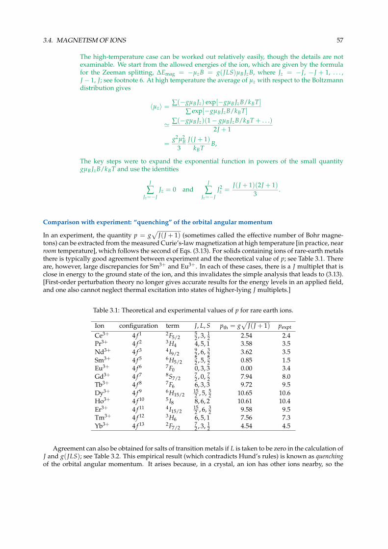
3.4. MAGNETISM OF IONS 57
The high-temperature case can be worked out relatively easily, though the details are notexaminable. We start from the allowed energies of the ion, which are given by the formulafor the Zeeman splitting, ∆Emag = −µzB = g(JLS)µB JzB, where Jz = −J, −J + 1, . . . ,J − 1, J; see footnote 6. At high temperature the average of µz with respect to the Boltzmanndistribution gives
〈µz〉 =∑(−gµB Jz) exp[−gµB JzB/kBT]
∑ exp[−gµB JzB/kBT]
' ∑(−gµB Jz)(1− gµB JzB/kBT + . . .)2J + 1
=g2µ2
B3
J(J + 1)kBT
B,
The key steps were to expand the exponential function in powers of the small quantitygµB JzB/kBT and use the identities
J
∑Jz=−J
Jz = 0 andJ
∑Jz=−J
J2z =
J(J + 1)(2J + 1)3
.
Comparison with experiment: “quenching” of the orbital angular momentum
In an experiment, the quantity p = g√
J(J + 1) (sometimes called the effective number of Bohr magne-tons) can be extracted from the measured Curie’s-law magnetization at high temperature [in practice, nearroom temperature], which follows the second of Eqs. (3.13). For solids containing ions of rare-earth metalsthere is typically good agreement between experiment and the theoretical value of p; see Table 3.1. Thereare, however, large discrepancies for Sm3+ and Eu3+. In each of these cases, there is a J multiplet that isclose in energy to the ground state of the ion, and this invalidates the simple analysis that leads to (3.13).[First-order perturbation theory no longer gives accurate results for the energy levels in an applied field,and one also cannot neglect thermal excitation into states of higher-lying J multiplets.]
Table 3.1: Theoretical and experimental values of p for rare earth ions.
Ion configuration term J, L, S pth = g√
J(J + 1) pexpt
Ce3+ 4 f 1 2F5/252 , 3, 1
2 2.54 2.4Pr3+ 4 f 2 3H4 4, 5, 1 3.58 3.5Nd3+ 4 f 3 4 I9/2
92 , 6, 3
2 3.62 3.5Sm3+ 4 f 5 6H5/2
52 , 5, 5
2 0.85 1.5Eu3+ 4 f 6 7F0 0, 3, 3 0.00 3.4Gd3+ 4 f 7 8S7/2
72 , 0, 7
2 7.94 8.0Tb3+ 4 f 8 7F6 6, 3, 3 9.72 9.5Dy3+ 4 f 9 6H15/2
152 , 5, 5
2 10.65 10.6Ho3+ 4 f 10 5 I8 8, 6, 2 10.61 10.4Er3+ 4 f 11 4 I15/2
152 , 6, 3
2 9.58 9.5Tm3+ 4 f 12 3H6 6, 5, 1 7.56 7.3Yb3+ 4 f 13 2F7/2
72 , 3, 1
2 4.54 4.5
Agreement can also be obtained for salts of transition metals if L is taken to be zero in the calculation ofJ and g(JLS); see Table 3.2. This empirical result (which contradicts Hund’s rules) is known as quenchingof the orbital angular momentum. It arises because, in a crystal, an ion has other ions nearby, so the
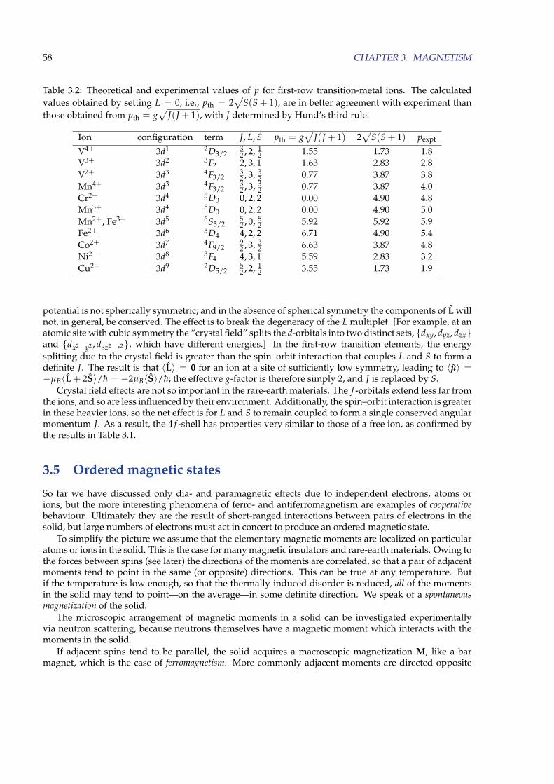
58 CHAPTER 3. MAGNETISM
Table 3.2: Theoretical and experimental values of p for first-row transition-metal ions. The calculatedvalues obtained by setting L = 0, i.e., pth = 2
√S(S + 1), are in better agreement with experiment than
those obtained from pth = g√
J(J + 1), with J determined by Hund’s third rule.
Ion configuration term J, L, S pth = g√
J(J + 1) 2√
S(S + 1) pexpt
V4+ 3d1 2D3/232 , 2, 1
2 1.55 1.73 1.8V3+ 3d2 3F2 2, 3, 1 1.63 2.83 2.8V2+ 3d3 4F3/2
32 , 3, 3
2 0.77 3.87 3.8Mn4+ 3d3 4F3/2
32 , 3, 3
2 0.77 3.87 4.0Cr2+ 3d4 5D0 0, 2, 2 0.00 4.90 4.8Mn3+ 3d4 5D0 0, 2, 2 0.00 4.90 5.0Mn2+, Fe3+ 3d5 6S5/2
52 , 0, 5
2 5.92 5.92 5.9Fe2+ 3d6 5D4 4, 2, 2 6.71 4.90 5.4Co2+ 3d7 4F9/2
92 , 3, 3
2 6.63 3.87 4.8Ni2+ 3d8 3F4 4, 3, 1 5.59 2.83 3.2Cu2+ 3d9 2D5/2
52 , 2, 1
2 3.55 1.73 1.9
potential is not spherically symmetric; and in the absence of spherical symmetry the components of L willnot, in general, be conserved. The effect is to break the degeneracy of the L multiplet. [For example, at anatomic site with cubic symmetry the “crystal field” splits the d-orbitals into two distinct sets, {dxy, dyz, dzx}and {dx2−y2 , d3z2−r2}, which have different energies.] In the first-row transition elements, the energysplitting due to the crystal field is greater than the spin–orbit interaction that couples L and S to form adefinite J. The result is that 〈L〉 = 0 for an ion at a site of sufficiently low symmetry, leading to 〈µ〉 =−µB〈L + 2S〉/h = −2µB〈S〉/h; the effective g-factor is therefore simply 2, and J is replaced by S.
Crystal field effects are not so important in the rare-earth materials. The f -orbitals extend less far fromthe ions, and so are less influenced by their environment. Additionally, the spin–orbit interaction is greaterin these heavier ions, so the net effect is for L and S to remain coupled to form a single conserved angularmomentum J. As a result, the 4 f -shell has properties very similar to those of a free ion, as confirmed bythe results in Table 3.1.
3.5 Ordered magnetic states
So far we have discussed only dia- and paramagnetic effects due to independent electrons, atoms orions, but the more interesting phenomena of ferro- and antiferromagnetism are examples of cooperativebehaviour. Ultimately they are the result of short-ranged interactions between pairs of electrons in thesolid, but large numbers of electrons must act in concert to produce an ordered magnetic state.
To simplify the picture we assume that the elementary magnetic moments are localized on particularatoms or ions in the solid. This is the case for many magnetic insulators and rare-earth materials. Owing tothe forces between spins (see later) the directions of the moments are correlated, so that a pair of adjacentmoments tend to point in the same (or opposite) directions. This can be true at any temperature. Butif the temperature is low enough, so that the thermally-induced disorder is reduced, all of the momentsin the solid may tend to point—on the average—in some definite direction. We speak of a spontaneousmagnetization of the solid.
The microscopic arrangement of magnetic moments in a solid can be investigated experimentallyvia neutron scattering, because neutrons themselves have a magnetic moment which interacts with themoments in the solid.
If adjacent spins tend to be parallel, the solid acquires a macroscopic magnetization M, like a barmagnet, which is the case of ferromagnetism. More commonly adjacent moments are directed opposite
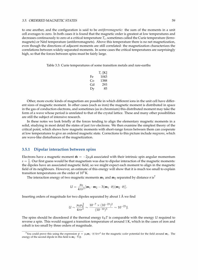
3.5. ORDERED MAGNETIC STATES 59
to one another, and the configuration is said to be antiferromagnetic: the sum of the moments in a unitcell averages to zero. In both cases it is found that the magnetic order is greatest at low temperatures anddecreases continuously to zero at a critical temperature Tc, sometimes called the Curie temperature (ferro-magnets) or Neel temperature (antiferromagnets). Above this temperature there is no net magnetization,even though the directions of adjacent moments are still correlated: the magnetization characterizes thecorrelations between widely-separated moments. In some cases the critical temperatures are surprisinglyhigh, so that the forces between spins must be fairly large.
Table 3.3: Curie temperatures of some transition metals and rare-earths
Tc [K]Fe 1043Co 1388Gd 293Dy 85
Other, more exotic kinds of magnetism are possible in which different ions in the unit cell have differ-ent sizes of magnetic moment. In other cases (such as iron) the magnetic moment is distributed in spacein the gas of conduction electrons, and sometimes (as in chromium) this distributed moment may take theform of a wave whose period is unrelated to that of the crystal lattice. These and many other possibilitiesare still the subject of intensive research.
In these notes we look briefly at the forces tending to align the elementary magnetic moments in asolid, studying in most detail the states of just two electrons. We then examine the simplest theory of thecritical point, which shows how magnetic moments with short-range forces between them can cooperateat low temperatures to give an ordered magnetic state. Corrections to this picture include magnons, whichare wave-like disturbances of the magnetization.
3.5.1 Dipolar interaction between spins
Electrons have a magnetic moment m = −2µB s associated with their intrinsic spin angular momentums = 1
2 . Our first guess would be that magnetism was due to dipolar interaction of the magnetic moments:the dipoles have an associated magnetic field, so we might expect each moment to align in the magneticfield of its neighbours. However, an estimate of this energy will show that it is much too small to explaintransition temperatures on the order of 103 K.
The interaction energy of two magnetic moments m1 and m2 separated by distance r is7
U =µ0
4πr3 [m1 ·m2 − 3(m1 · r)(m2 · r)].
Inserting orders of magnitude for two dipoles separated by about 1 A we find
U ∼µ0µ 2
B4πr3 ∼
10−7 × (10−23)2
(10−10)3 ∼ 10−23 J.
The spins should be disordered if the thermal energy kBT is comparable with the energy U required toreverse a spin. This would suggest a transition temperature of around 1 K, which in the cases of iron andcobalt is too small by three orders of magnitude.
7You could prove this using the expression ψ = µ0m1 · r/4πr2 for the magnetic scalar potential for the field around m1. Theenergy of the second dipole in this field is m2 · ∇ψ.
60 CHAPTER 3. MAGNETISM
3.5.2 Exchange interaction
In fact, the mechanism for spin alignment in magnets comes about indirectly as a result of electrostatic in-teractions and the antisymmetry of electron wave functions Φ(r1σ1, r2σ2, . . .) = −Φ(r2σ2, r1σ1, . . .), whichis a fundamental property of all fermion wave functions. This is the general rule that leads to Pauli’sexclusion principle. For if two electrons are known to be in states α and β, the only antisymmetric combi-nation of these is
Φ(1, 2) = α(1)β(2)− α(2)β(1),
where the symbols (1) and (2) are just a shorthand for (r1σ1) and (r2σ2), or whatever variables the statesare supposed to depend on. If the two states α and β are the same Φ(1, 2) vanishes, so two electronscannot occupy the same state.
To the extent that spin–orbit coupling can be neglected, the interaction between two electrons is sim-ply the Coulomb interaction e2/4πε0r12, and can be included in the Hamiltonian H(1, 2) along with thekinetic and single-particle potential energies. Because the energy is symmetrical and does not depend onthe spin variables, solutions of the purely spatial Schrodinger equation,
Hψ(r1, r2) = Eψ(r1, r2),
which determine the energy levels of the two electrons, are themselves either symmetric or antisymmetric:ψ(1, 2) = ±ψ(2, 1). [This is easy to see for a non-degenerate level as ψ(1, 2) and ψ(2, 1) each solve thesame Schrodinger equation. If the level is non-degenerate, the two functions must be identical apart froma factor, ψ(2, 1) = Cψ(1, 2). Repeating the argument gives ψ(1, 2) = C2ψ(1, 2), so that C = ±1.]
This is consistent with the Pauli principle because the complete wave function
Φ(1, 2) = ψ(r1, r2) χ(σ1, σ2) (3.14)
is the product of space- and spin-dependent functions, so if ψ is symmetric, χ will be antisymmetric, andvice versa.
If we are interested in only a few low-energy states of a system that can be specified uniquely by theirspin configuration it is sometimes convenient to reverse the argument. The spin state determines thesymmetry of the spatial state, and this in turn determines the energy, via Schrodinger’s equation. Thisdependence of the energy on the spin state is known as the exchange interaction.
We can see how the exchange interaction leads to Hund’s first rule for electrons in spatial states a andb, assumed to be degenerate in energy when electron interactions are neglected. (The functions a andb might be two atomic p orbitals, as in an atom of carbon.) There is only one antisymmetric spin wavefunction for two electrons,
χs = (↑1↓2 − ↓1↑2)/√
2 .
This “singlet” state has total Sz = 0, and so must correspond to total S = 0. The corresponding symmetricspatial wave function is
ψs = (a(1)b(2) + b(1)a(2))/√
2 . (3.15)
On the other hand there is a “triplet” of states with symmetrical spin wave functions
χt =
↑1↑2
(↑1↓2 + ↓1↑2)/√
2↓1↓2 .
(3.16)
They have, respectively, Sz = 1, 0 and −1, and so correspond to S = 1. For all three, the antisymmetricspatial wave function is
ψt = (a(1)b(2)− b(1)a(2))/√
2 , (3.17)
which vanishes when r1 = r2. Thus, the probability of finding the two electrons close together is smallerin the triplet state than in the singlet; the expectation value of the electron–electron interaction is reduced,
3.5. ORDERED MAGNETIC STATES 61
so that the triplet has lower energy than the singlet. This is the origin of Hund’s first rule for the couplingof spins, as it prefers S = 1 over S = 0.
Suppose that Es > Et are the energies of the singlet and triplet states. In this case we can (in a purelyad hoc way) write the energy as a function of the total spin S,
Eeff(S) = Es − 12 (Es − Et)S(S + 1) =
{Es for S = 0Et for S = 1.
(3.18)
The function E(S) has been written in terms of S(S + 1) for a reason: S(S + 1)h2 are the eigenvalues ofthe square of the operator for the total spin of the two electrons, so that (3.18) shows that Es and Et are theeigenvalues of an effective spin-Hamiltonian,
Heff = Es − 12 (Es − Et)S2/h2 .
The expression for Heff can be written explicitly in terms of the operators for the individual spins,
S2 = (s1 + s2)2
= s21 + s2
2 + 2s1 · s2
= 32 h2 + 2s1 · s2
where to get the last result we have used s21 = s2
2 = 34 h2. Putting these results together we find that the
effective Hamiltonian can be written in the form
Heff(s1, s2) = const. + Js1 · s2/h2, (3.19)
where the coupling constant, J = (Et − Es) < 0, is the singlet–triplet energy difference [Heisenberg 1926,Dirac 1929]. Within an atom, J is on the order of one electron volt, which is much greater than the dipolarinteraction energy.
Exercise 3.7:
Verify the result in (3.19) and find the value of the additive constant in terms of Es and Et.
Given the form of the singlet and triplet spatial wave functions (3.15) and (3.17) we can use first-orderperturbation theory to estimate the energy-splitting of the singlet and triplet states. The results are [inatomic units, e2/4πε0 = 1]⟨
1r12
⟩s=∫ ∫ |a(1)|2|b(2)|2
r12d3r1 d3r2 +
∫ ∫ a∗(1)b∗(2)a(2)b(1)r12
d3r1 d3r2
≡ UD[a, b] + UX [a, b]
⟨1
r12
⟩t= UD[a, b]−UX [a, b] .
UD and UX are known, respectively, as the direct and exchange energies. The direct energy can be in-terpreted as the electrostatic interaction energy of two charge distributions −e|a(r)|2 and −e|b(r)|2. Thedifference in sign of the exchange energy in the singlet and triplet states can be traced directly to thesymmetry and antisymmetry of the spatial wave functions.
Exercise 3.8:
Optional. Show that UX is always positive. [Regard UX as the energy of interaction of twocomplex conjugate charge distributions ρ(1) = a(1)b∗(1) and ρ∗(2) = a∗(2)b(2) and separate ρ,ρ∗ and UX into real and imaginary parts. The imaginary part of UX vanishes, and the real partcan be recognised as the sum of the (positive) electrostatic energies of Re ρ and Im ρ.]
62 CHAPTER 3. MAGNETISM
3.5.3 Exchange interaction between ions
So far we have seen that the exchange interaction makes it favourable for electron spins to align withinan atom, and so leads to Hund’s rule (H1). Interactions of the same general kind are responsible for theinteraction between the spins on different ions in a magnetic solid.
The expression for the exchange energy UX depends on the product a∗(r)b(r), and so is small if theorbitals a(r) and b(r) overlap only slightly, as is the case for electrons belonging to different ions. Com-pared with the interactions between electron spins within an ion, the interactions between the total spinsof different ions should correspond to smaller values of exchange coupling constant J. A critical tempera-ture of 103 K in a magnetic solid would suggest |J| ∼ 0.1 eV, which is indeed substantially less than in theintraatomic |J| ∼ 1 eV responsible for Hund’s first rule.
3.5.4 Why aren’t all magnets FM?
The picture we have just described cannot be complete, otherwise all magnets would be ferromagnetic.There are several complications to the picture.
Indirect exchange interaction
In the case of rare earth elements (the lanthanides) the picture of localized spins is correct (they are locatedin the f -orbitals), but the orbitals are too tightly bound to the atoms to allow a simple exchange interaction.The interaction in this case occurs indirectly, via the conduction electrons of the solid.
Roughly speaking, there is a simple exchange interaction between the conduction electrons and thef electrons in the rare-earth ion. Up- and down-spin conduction electrons are attracted by differentamounts to the ion. The resulting shift in phase between the wave functions of up and down electronscauses one or the other to predominate at any given point in space. It can be shown (using second-orderperturbation theory) that the difference n↑ − n↓ oscillates as a function of position, where the oscillationshave wave vector 2kF; kF is the Fermi wave vector of the gas of conduction electrons. As a result, theenergy of a second rare-earth ion immersed in the conduction-electron sea has an oscillatory dependenceon its distance R from the first ion,
E(S1, S2) = JS1 · S2 with J ∼ const.× cos(2kFR)R3 .
This is the Rudermann–Kittel interaction, or indirect exchange.Whether the solid is ferro- or antiferromagnetic depends on the sign of the coupling constant J, which
in turn depends on the separation of the magnetic ions, and on the conduction electron density via kF.Both kinds of magnetism (and more) have been observed among the rare-earth metals and their alloys.
Superexchange interaction
In the electrically-insulating oxides of transition metals, such as manganese oxide, a slightly differentmechanism is reponsible for the alignment of the spins of the transition-metal ions.
Manganese oxide is antiferromagnetic at temperatures below 116 K. In the crystal, Mn2+ and O2− ionsoccupy alternate sites of a simple-cubic lattice. [The lattice type is therefore cubic-F, with one Mn andone O ion per lattice point.] The manganese ions have a magnetic moment, due to the electrons in thehalf-filled 3d shell, but the ions are too far apart for the 3d wave functions to have any significant overlap,so the normal exchange interaction would be too small to explain the ordering of the spins; moreover, itwould be of the wrong sign to give an antiferromagnetic interaction. Instead, the interaction arises via theexchange interaction with the electrons on the magnetically-inert oxygen ions. An oxygen p-electron canmake virtual transitions into states of one of its neighbouring Mn ions, leaving an electron behind thatcan interact (via the exchange interaction) with a 3d electron of another Mn ion.8
8An appeal to “virtual transitions” is usually a metaphor for an effect that can be understood by using second-order perturbationtheory. The theory was worked out in detail by P. W. Anderson [1950], though it was not the work that won him a Nobel prize.
3.6. FERROMAGNETIC GROUNDSTATE AND EXCITATIONS 63
Indirect interactions of this kind, via the electrons of non-magnetic ions, are usually called superex-change; they can be either ferromagnetic or (more commonly) antiferromagnetic, as in MnO. The threepossibilities for exchange discussed above are illustrated in Figure.
3.5.5 The Heisenberg Hamiltonian
Regardless of the details of the exchange mechanism, the low-energy states of a magnetic material withlocalized spins are often described by the Heisenberg Hamiltonian,
HHeis = ∑〈i,j〉
Jij Si · Sj/h2 , (3.20)
where Si denotes the operator for the total spin of the ith ion (which need not be 12 ) and the notation 〈i, j〉
means that the sum is taken over distinct pairs of ions i and j.Although the Heisenberg Hamiltonian has often been used as the starting point for theoretical discus-
sions of magnetism, it should not be regarded as fundamental. It can be derived by perturbation theoryin some cases [footnote 8], but the approximations involved are rarely under “good control”: there is notalways a suitable small parameter to expand in. Equation (3.20) is perhaps better regarded as the simplestHamiltonian that respects the fact that the ionic spins are quantum-mechanical and can interact via oneof the exchange mechanisms. We shall use it here without further discussion.
3.6 Ferromagnetic groundstate and excitations
Besides being used to characterize the magnetic order in a solid, neutron scattering can also be used tostudy magnetic excitations. The neutrons are coupled to the magnetization density via their own magneticmoments, and are scattered with loss (or gain) of energy corresponding to creation (or absorption) ofthese excitations. Measurement of the energy change as a function of the change in the neutron wavevector gives the dispersion relation of the excitations: crystal momentum and energy are conserved in theinteractions.
The excitations of lowest energy are called magnons, and correspond classically to propagating wave-like disturbances of the magnetization in the solid, rather as phonons correspond classically to soundwaves. A classical derivation of the spin-wave spectrum is surprisingly involved [the details are given byKittel], so instead we take the easier route of looking at the excited states of a one-dimensional ferromag-netic chain of quantum-mechanical spins with s = 1
2 , each of which is coupled to its neighbours by theexchange interaction. The Heisenberg model Hamiltonian is
H = −|J|h2 ∑
nSn · Sn+1,
where n runs over all N spins in the chain, and the exchange coupling constant has been written as −|J|to emphasize the fact that the interaction is ferromagnetic, and so tends to align the spins.
3.6.1 Groundstate energy
All the spins are parallel in a state of lowest energy; one state of this kind is
χ(0) = ↑1↑2 . . . ↑N−1↑N ;
it has total Sz =12 N, the largest possible value for N spins- 1
2 .To work out the energy, we first apply any one of the terms Sn · Sn+1 to χ(0); for example, the term
with n = 1. Now, S1 · S2 can be rewritten9
S1 · S2 = 12{
S212 − S2
1 − S22}
,
9Recall the “trick” of replacing L · S by 12
{J2 − L2 − S2} to work out its eigenvalues in terms of the quantum numbers J, L and S.
64 CHAPTER 3. MAGNETISM
where S12 ≡ S1 + S2. Like the square of any angular momentum operator, the eigenvalues of S212 are
S12(S12 + 1)h2, where S12 = 1 in the state χ(0) because the two spins are parallel [see Eq. (3.16), first line].On the other hand,
S21 = S1(S1 + 1) h2 = 3
4 h2,
because S1 = 12 ; similarly, we can replace S2
2 by 34 h2.
Putting the last results together, we find
S1 · S2 χ(0) = 12{1× (1 + 1)h2 − 2× 3
4 h2}χ(0) = 14 h2χ(0),
and we can argue in the same way for any pair of spins in the chain. Finally we obtain
Hχ(0) = −|J|h2
N
∑n=1
Sn · Sn+1 χ(0) = − 14 N|J|χ(0), (3.21)
which shows that χ(0) is an eigenstate of H with energy eigenvalue E(0) = − 14 N|J|.
It is worth pointing out that the ground “state” is actually highly degenerate: the total spin S = 12 N,
so the degeneracy is 2S + 1 = N + 1, corresponding to the possible values of Sz = −S, −S + 1, . . . ,S− 1, S. A closely-related point should also be understood: the Hamiltonian has full rotational symmetry(it depends only on the scalar products Sn · Sn+1), but the state χ(0) lacks this symmetry, because allthe spins are pointing along the z-axis. In this and similar cases we say that the groundstate has brokensymmetry.
3.6.2 Spin-flip excitations and magnons
The basic excitation can be taken to be a “spin-flip”, i.e., a state which differs from the ground state by thereversal of one spin on the nth site,
χn = ↑1 . . . ↑n−1↓n↑n+1 . . . ↑N .
The total Sz in this state is 1 less than in the ground state. By itself the spin-flip is not a solution of Schro-dinger’s equation. We can understand this in much the same way that we worked out the ground stateenergy in the last section,10 by considering the result of applying Sm · Sm+1 to χn.
Provided m 6= n− 1 or n, Sm and Sm+1 will both be acting on up-spins, so the result is the same as inthe groundstate:
Sm · Sm+1χn = 14 h2χn for m 6= n− 1 or n; (3.22)
but if m = n we must consider the effect of Sn · Sn+1 on ↓n↑n+1. To simplify the calculation, we note that
↓n↑n+1 = 12(↓n↑n+1 − ↑n↓n+1
)+ 1
2(↓n↑n+1 + ↑n↓n+1
)is a linear combination of the singlet state (spin 0) with one of the triplet states (spin 1). Just as in thecalculation of the groundstate energy, we rewrite Sn · Sn+1 in terms of its square, so that
Sn · Sn+1 ↓n↑n+1 = 12
{(Sn + Sn+1
)2 − 32 h2
} [12(↓n↑n+1 − ↑n↓n+1
)+ 1
2(↓n↑n+1 + ↑n↓n+1
)]= 1
4
[{0× 1 h2 − 3
2 h2}(↓n↑n+1 − ↑n↓n+1)+{
1× 2 h2 − 32 h2}(↓n↑n+1 + ↑n↓n+1
)]= − 1
4 h2 ↓n↑n+1 +12 h2 ↑n↓n+1,
which gives, after inserting the states ↑m for the remaining N − 2 spins,
Sn · Sn+1 χn = − 14 h2 χn +
12 h2 χn+1. (3.23)
10The key result in this subsection is (3.25); the steps that lead up to it are not examinable. Nevertheless, if you are interested, amore sophisticated (and algebraically simpler) approach to this problem is given in Aschroft & Mermin, Solid State Physics, equation(33.19) onwards; also in Lifshitz & Pitaevskii, Statistical Physics, Part 2, Sec. 72.
3.6. FERROMAGNETIC GROUNDSTATE AND EXCITATIONS 65
In a very similar way one can show that
Sn−1 · Sn χn = − 14 h2 χn +
12 h2 χn−1. (3.24)
After putting the results of (3.22), (3.23) and (3.24) together and summing over m, we find
Hχn = −|J|h2
N
∑m=1
Sm · Sm+1 χn
= E(0)χn + |J|(χn − 1
2 χn+1 − 12 χn−1
). (3.25)
In words, the effect of H is to transfer a spin-flip on site n to the neighbouring sites n± 1. This soundsvery similar to the description of an electron tunnelling between atoms in the tight-binding model, thoughit should be emphasized that it is a spin-flip, rather than an actual particle, which is in motion here.
Magnon dispersion relation
The close analogy with the tight-binding model makes it easy to find a wave function that describes apropagating spin-flip. First we construct a Bloch function φk from the states χn,
φk =N
∑m=1
eikma χm .
We apply H to φk, which (after using (3.25)) gives
Hφk =(E(0) + |J|
)φk − 1
2 |J|N
∑m=1
eikma(χm+1 + χm−1) . (3.26)
Provided the chain of spins is closed (so that χN+1 ≡ χ1), the first sum in (3.26) can be completed bymaking a change of variable n = m + 1:
N
∑m=1
eikmaχm+1 =N+1
∑n=2
eik(n−1)aχn ≡ e−ikaφk .
Similarly, by making the change of variable n = m− 1,
N
∑m=1
eikmaχm−1 ≡ eikaφk .
Using these last two results in (3.26) finally gives
Hφk =[E(0) + |J| − 1
2 |J|e−ika − 1
2 |J|eika] φk
=[E(0) + |J| (1− cos ka)
]φk ,
showing that φk is a solution of Schrodinger’s equation with energy slightly greater than the groundstateenergy E(0). We can interpret the excess energy as the energy
εk = |J|(1− cos ka) (3.27)
of a magnon with crystal momentum hk. Note that the result for εk is very similar to the energy E(k) ofan electron in a tight-binding model with hopping between nearest neighbours; see (2.21).
66 CHAPTER 3. MAGNETISM
Exercise 3.9:
Check that you understand (and can reproduce) all the steps leading from (3.25) to (3.27).
For long wavelengths (k→ 0) the dispersion relation of the magnon is similar to that of a free particle,εk ' 1
2 |J|k2a2. Neutron scattering data from iron, cobalt and nickel suggest a magnon dispersion of thesame form Ak2, with A ' 0.3–0.5 eV A2. This would be consistent with an exchange coupling constant|J| in the range 0.1–0.2 eV, as would also be required for a critical temperature in excess of 1000 K. Never-theless, it should be borne in mind that the model is not precisely comparable with experiment here. Themagnetization density in these metals is distributed in the gas of conduction electrons, rather than beinglocated solely on the ions as required by the model.
In antiferromagnets the long-wavelength dispersion relation is found experimentally to be linearrather than quadratic, E ∝ k. An analysis starting from Schrodinger’s equation is more difficult here,and we do not attempt it.11 In fact, it is a far from trivial task to work out even the ground state wavefunction of the 1D Heisenberg antiferromagnet: it is not the “obvious” state . . . ↑↓↑↓ . . . that one mighthave guessed by analogy with the ferromagnet.
Effect of magnons on the magnetization at low temperature
Experimentally, the magnetization, M(T), of a ferromagnet is found to follow a power law at low tem-peratures,
[M(0)−M(T)] ∝ T3/2.
The reason for the power law dependence on T is the presence of low-energy magnetic excitations, evenat the lowest temperatures. These excitations are the long-wavelength magnons, for which εk ' Ak2.Each magnon has sz = −1 (it corresponds to a single delocalized spin-flip), so that as the temperaturerises the magnetization decreases in proportion to the number of magnons present.
Now, we expect a given spin-wave mode of the solid to be thermally excited if the magnon energyis less than about kBT, so here we expect all modes to be excited up to kmax, where Akmax
2 ' kBT,or kmax ∝ T1/2. The total number of excited modes is proportional to the volume of reciprocal spacewith k < kmax; this volume is in turn proportional to kmax
3, or T3/2. The power-law dependence ontemperature is usually known as Bloch’s T3/2 law.12
Exercise 3.10:
Optional: see Q. 3 on the final examples sheet for PHYS30151. The above argument for the T3/2
law takes no account of the fact that different modes contain different numbers of magnons.Correct the argument on the assumption that magnons are non-interacting, non-conservedbosons, so that the average number with wave vector k follows the Bose–Einstein distributionlaw,
〈nk〉 =1
e εk/kBT − 1,
with chemical potential µ = 0.
3.7 Mean-field theory of the critical point
So far we have discussed the magnetization only at low temperature. As the temperature rises towards Tc,the magnetization steadily decreases to zero as illustrated in Fig., and it is zero at all temperatures aboveTc. This general behaviour is not intuitively obvious, and it requires an explanation: why shouldn’t themagnetization remain non-zero for all temperatures, tending to zero only for T → ∞? Alternatively, why
11A classical treatment is given in Kittel’s textbook, if you are interested.12Not to be confused with his T5 law for the phonon-induced electrical resistivity in metals.
3.7. MEAN-FIELD THEORY OF THE CRITICAL POINT 67
shouldn’t it jump discontinuously to zero at the critical temperature? These things, at least, we will be ableto explain. We should also like (over-optimistically, it turns out) to understand some of the details of thetemperature dependence. For example, just below the critical temperature it is found experimentally that
M(T) ∝ (Tc − T)β,
with β ' 0.33 typically; the power β is a particular case of a critical exponent. In large, homogeneoussamples the magnetic susceptibility of a ferromagnet diverges as
χ(T) ∝ |Tc − T|−γ,
defining another critical exponent γ which typically lies in the range 1.2–1.3. Indeed, all of the macro-scopic, thermodynamic quantities show some kind of unusual behaviour at the critical point. Our aim isto understand this at the simplest level of approximation, so we should not be too concerned if some ofthe details turn out to be wrong.
Making the mean-field approximation
To get a simple picture of the ferromagnetic phase transition we can make a mean-field approximation, inwhich the effect of the neighbours of a given spin s0 is replaced by an average.
In the magnetic state, the average magnetic moment of a spin is non-zero:
〈µi〉 = −gµB〈si〉/h 6= 0 , (3.28)
where the angled brackets denote the usual thermal average. If all the spins have the same atomic envi-ronment this average will be the same for every spin: 〈µi〉 ≡ 〈µ〉, independent of i.
Any given spin tends, on average, to point in the same direction as its neighbours; this is the result ofthe ferromagnetic Heisenberg exchange interaction, which favours the alignment of the spins. Focus, forthe moment, on a particular spin, s0, with n nearest neighbours; its energy is
E = −|J|h2
n
∑j=1
s0 · sj = −n|J|h2 s0 ·
[∑n
j=1 sj
n
]
≡ − n|J|g2µ2
Bµ0 ·
[∑n
j=1 µj
n
]
' − n|J|g2µ2
Bµ0 · 〈µj〉 , (3.29)
where, in the last line, we have replaced the average over the n nearest neighbours by the average overthe whole solid: this replacement is the mean-field approximation. It certainly cannot be exact, but we mighthope that it would be a reasonably good approximation when n is large. Typical values of n are 8 or 12,for the BCC and FCC structures, respectively.
We can re-write (3.29) in the same form as the interaction of a spin with a effective magnetic field, Beff,
E ' −µ0 ·(
n|J|g2µ2
B〈µj〉
)≡ −µ0 · Beff . (3.30)
From this point onward, we shall assume, for simplicity, that the spins have s = 12 , so that g = 2; we also
assume that 〈µ〉 and Beff are in the z-direction. With these assumptions, the magnitude of the effectivefield will be
Beff =n|J|4µ2
B〈µz〉 . (3.31)
68 CHAPTER 3. MAGNETISM
The mean-field magnetization
The energy of a spin in a magnetic field B in the z-direction is E = ∓µB B, the two values correspondingto µz = ±µB. In Section 3.3.1 we found the thermal average of the magnetic moment to be given by
〈µz〉 = µB tanh[µBB/kBT] ; (3.32)
we now simply replace B by Beff [defined in (3.31] and introduce a temperature scale Tc, defined bykBTc ≡ n|J|/4. [The notation anticipates the result, of course: Tc will turn out to be the critical temperaturein the mean-field approximation.] After making these replacements in (3.32) we find
〈µz〉/µB = tanh[
Tc 〈µz〉/µBT
]. (3.33)
The quantity 〈µz〉/µB ≡ m is a scaled magnetic moment, which takes values between −1 and 1. In termsof m, the last equation can be written
m = tanh[Tc m/T] , (3.34)
which is the basic equation of the mean-field approximation for a spin-half ferromagnet. In principle, wecan solve it to obtain m(T).
Temperature dependence of m
We can predict the general behaviour of m(T) by a graphical method. First we rearrange (3.34) as
arctanh m = m Tc/T . (3.35)
Each side of the equation can be sketched as a function of m; the solution m(T) is given by the intersectionof the two curves.
If T is too large, the straight line y = m Tc/T falls below the curve y = arctanh m, and the only solutionof (3.35) is the trivial one, m = 0. In this case (high temperature) the expected magnetization is zero.
On the other hand, if T is small the two curves intersect three times. The new solutions with m 6= 0correspond to a spontaneous magnetization that increases with decreasing T. There is a definite criticaltemperature Tc at which this magnetization appears, and we can calculate the behaviour of the magneti-zation when it is small, at temperatures just below Tc. Using the series expansion arctanh m ' m + 1
3 m3,valid for small m, we find
m + 13 m3 ' m Tc/T .
After dividing through by m (we ignore the trivial solution m = 0) and rearranging a little, we find
13 m2 ' Tc
T− 1 or m2 ' 3(Tc − T)/T ,
which is zero when T = Tc. Just below the transition, therefore, the magnetization varies as (Tc − T)1/2.This is a definite prediction of the mean-field theory: the critical exponent for the magnetization is β = 1
2 .It does not agree very well with the value β ' 0.33 seen in experiment.
The observed deviations from mean-field theory at the critical point are significant and a great deal ofexperimental and theoretical work has been done to clarify their origin. This is a useful thing to do becausethe critical behaviour is fairly insensitive to the details of the interactions between magnetic moments, sothat many different magnetic solids have the same critical exponents. It is difficult, unfortunately, to givea short, qualitative account of precisely how the theoretical description of the critical point has been putinto agreement with experiment.
The real value of the mean-field approximation is its simplicity and generality, rather than its accuracy,so that it can provide a qualitative understanding of even quite complicated magnetic systems. Neverthe-less, the mean field theory has been found to be quantitatively accurate for at least one material, HoRh4B4.
3.7. MEAN-FIELD THEORY OF THE CRITICAL POINT 69
It is an alloy containing rare-earth ionic spins, whose interactions with one another is probably best de-scribed by the Rudermann–Kittel interaction. The coupling constant J is thought to take the same sign forthe interaction of a spin with a large number of its neighbours, not just the ones nearest to it in the crys-tal lattice. In this case the sum ∑n
j=1 µj is unusually well approximated by n〈µ〉, because the interactionsamples many more than 8 or 12 spins. Even so, we should expect more accurate experiments to showdeviations from the mean-field behaviour at temperatures very close to the critical point.
Other weaknesses of mean-field theory
Mean-field theory also makes an incorrect prediction for the behaviour of the magnetization at tempera-tures well below Tc. In this regime (3.34) reduces to
〈m(T)〉 ' 1− 2 e−2Tc/T , or [M(0)−M(T)] ∝ e−2Tc/T ,
so that the curve of magnetization as a function of temperature can be expected to be very flat in theregion T � Tc. But as we have discussed before, the low temperature magnetization is actually observedto follow a power law,
[M(0)−M(T)] ∝ T3/2,
which is entirely different from the mean-field prediction, but which we have explained by the presenceof low-energy excitations (the long-wavelength magnons) at low temperature. These excitations are com-pletely ignored by the mean-field approximation.
The situation just described is reminiscent of what happens with the heat capacity of a non-magnetic insulating solid at low temperature. The Debye theory of the specific heat shows—and experiments agree—that C(T) varies as T3, because at low temperatures the thermalproperties are dominated by long-wavelength phonons, which are the only low-energy ex-citations of an insulator. Like mean-field theory, the simpler Einstein model of a solid in-correctly predicts that C(T) vanishes as exp[−Θ/T] at low temperatures, where Θ is a char-acteristic temperature. You could, in fact, think of Einstein’s model as being a mean-fieldapproximation in which each atom vibrates independently in an averaged, harmonic po-tential due to its neighbours. This potential is the same for every atom, so the vibrationalfrequency ωE is the same for each atom; the characteristic temperature is then related to thisfrequency by Θ ∼ hωE/kB.
Total energy and heat capacity in the mean-field approximation
This was not covered in the lectures in 2017, so the topic is not examinable this year.