solarwind:Turbulenceand solarwind acceleration

Astronomy & Astrophysics manuscript no. 39872corrcorr c©ESO 2021January 14, 2021

Letter to the Editor

The near-Sun streamer belt solar wind: Turbulence and solar wind acceleration

C. H. K. Chen1, B. D. G. Chandran2, L. D. Woodham3, S. I. Jones4, J. C. Perez5, S. Bourouaine5, 6, T. A.Bowen7, K. G. Klein8, M. Moncuquet9, J. C. Kasper10, 11, S. D. Bale1, 3, 7, 12

1 School of Physics and Astronomy, Queen Mary University of London, London E1 4NS, UKe-mail: [email protected]

2 Department of Physics and Astronomy, University of New Hampshire, Durham, NH 03824, USA3 Department of Physics, Imperial College London, London SW7 2AZ, UK4 NASA Goddard Space Flight Center, Greenbelt, MD 20771, USA5 Department of Aerospace, Physics and Space Sciences, Florida Institute of Technology, Melbourne, FL 32901, USA6 Johns Hopkins University Applied Physics Laboratory, Laurel, MD 20723, USA7 Space Sciences Laboratory, University of California, Berkeley, CA 94720, USA8 Lunar and Planetary Laboratory, University of Arizona, Tucson, AZ 85719, USA9 LESIA, Observatoire de Paris, Université PSL, CNRS, Sorbonne Université, Université de Paris, 92195 Meudon, France

10 Climate and Space Sciences and Engineering, University of Michigan, Ann Arbor, MI 48109, USA11 Smithsonian Astrophysical Observatory, Cambridge, MA 02138 USA12 Physics Department, University of California, Berkeley, CA 94720, USA

January 14, 2021

ABSTRACT

The fourth orbit of Parker Solar Probe (PSP) reached heliocentric distances down to 27.9 R�, allowing solar wind turbulence andacceleration mechanisms to be studied in situ closer to the Sun than previously possible. The turbulence properties were found to besignificantly different in the inbound and outbound portions of PSP’s fourth solar encounter, which was likely due to the proximity tothe heliospheric current sheet (HCS) in the outbound period. Near the HCS, in the streamer belt wind, the turbulence was found tohave lower amplitudes, higher magnetic compressibility, a steeper magnetic field spectrum (with a spectral index close to –5/3 ratherthan –3/2), a lower Alfvénicity, and a ‘1/ f ’ break at much lower frequencies. These are also features of slow wind at 1 au, suggestingthe near-Sun streamer belt wind to be the prototypical slow solar wind. The transition in properties occurs at a predicted angulardistance of ≈ 4◦ from the HCS, suggesting ≈ 8◦ as the full-width of the streamer belt wind at these distances. While the majority ofthe Alfvénic turbulence energy fluxes measured by PSP are consistent with those required for reflection-driven turbulence models ofsolar wind acceleration, the fluxes in the streamer belt are significantly lower than the model predictions, suggesting that additionalmechanisms are necessary to explain the acceleration of the streamer belt solar wind.

Key words. solar wind – Sun: heliosphere – plasmas – turbulence – waves

1. Introduction

One of the major open questions in heliophysics is how the so-lar wind is accelerated to the high speeds measured in situ byspacecraft in the Solar System (Fox et al. 2016). Early mod-els of solar wind generation, based on the pioneering work ofParker (1958), were able to reproduce the qualitative propertiesof the solar wind, although they could not explain all of the mea-sured quantities seen at 1 au (see, e.g. the reviews of Parker1965; Leer et al. 1982; Barnes 1992; Hollweg 2008; Hansteen& Velli 2012; Cranmer et al. 2015, 2017). Turbulence is nowthought to be one of the key processes playing a role in solarwind acceleration, providing both a source of energy to heat thecorona (Coleman 1968) and a wave pressure to directly acceler-ate the wind (Alazraki & Couturier 1971; Belcher 1971). Possi-ble mechanisms for the driving of the turbulence include reflec-tion of the outward-propagating Alfvén waves by the large-scalegradients (Heinemann & Olbert 1980; Velli 1993) and velocityshears (Coleman 1968; Roberts et al. 1992). Models that incor-porate these effects are now able to reproduce most solar wind

conditions at 1 au (e.g. Cranmer et al. 2007; Verdini et al. 2010;Chandran et al. 2011; van der Holst et al. 2014; Usmanov et al.2018; Shoda et al. 2019), but more stringent tests come fromcomparing their predictions to measurements close to the Sun.

The nature of the turbulence in the solar wind and plasma tur-bulence in general is also a major open question (Bruno & Car-bone 2013; Alexandrova et al. 2013; Kiyani et al. 2015; Chen2016). Initial results from Parker Solar Probe (PSP) have re-vealed many similarities, but also some key differences in thenear-Sun solar wind turbulence. Both the power levels and cas-cade rates were found to be several orders or magnitude largerat ∼ 36 R� compared to 1 au (Bale et al. 2019; Chen et al. 2020;Bandyopadhyay et al. 2020). The turbulence was also found tobe less magnetically compressible and more imbalanced, with ashallower magnetic field spectral index of ≈ −3/2. The low com-pressibility and polarisation is consistent with a reduced slowmode component to the turbulence (Chen et al. 2020; Chastonet al. 2020). Both the outer scale and ion scale spectral breaksmove to larger scales approximately linearly with heliocentricdistance (Chen et al. 2020; Duan et al. 2020), indicating that the

Article number, page 1 of 7

Article published by EDP Sciences, to be cited as https://doi.org/10.1051/0004-6361/202039872Article published by EDP Sciences, to be cited as https://doi.org/10.1051/0004-6361/202039872Article published by EDP Sciences, to be cited as https://doi.org/10.1051/0004-6361/202039872

http://publications.edpsciences.org/

https://doi.org/10.1051/0004-6361/202039872


https://doi.org/10.1051/0004-6361/202039872


https://doi.org/10.1051/0004-6361/202039872

A&A proofs: manuscript no. 39872corrcorr

-100

0

100

500

1000

1500

200

400

600

100

200

300

0

2

4

6

012345

10-1

100

101

102

103

-10

-5

0

024 025 026 027 028 029 030 031 032 033 034 035

30

40

50

Fig. 1. Time series of Encounter 4 solar wind parameters: Magnetic fieldB in RTN coordinates (blue=radial, red=tangential, yellow=normal,purple=magnitude), electron density ne, solar wind speed vi, ion temper-ature Ti, mass flux 4πρvrr2, energy flux 2πρv3

r r2, ion beta βi, predictedangular distance to the heliospheric current sheet φHCS, and radial dis-tance r. The vertical dashed lines indicate the intervals used to calculatethe spectra in Figure 6.

width of the magnetohydrodynamic (MHD) inertial range staysapproximately constant over this distance range. The steep ion-scale transition range, however, is more prominent closer to theSun, indicating stronger dissipation or an increase in the cascaderate (Bowen et al. 2020), or perhaps a build-up of energy at thesescales (Meyrand et al. 2020). The overall increase in the turbu-lence energy flux, compared to the bulk solar wind kinetic energyflux, was found by Chen et al. (2020) to be consistent with thereflection-driven turbulence solar wind model of Chandran et al.(2011), showing that this remains a viable mechanism to explainthe acceleration of the open field wind. Other comparisons ofthe early PSP data to turbulence-driven models also report agree-ment (Bandyopadhyay et al. 2020; Réville et al. 2020a; Adhikariet al. 2020).

Much of the solar wind measured in the early PSP solar en-counters has been of open-field coronal hole origin (Bale et al.2019; Panasenco et al. 2020; Badman et al. 2020a,b), althoughshort periods of streamer belt wind near the heliospheric currentsheet (HCS) were also identified (Szabo et al. 2020; Rouillardet al. 2020; Lavraud et al. 2020). Encounter 4, however, wasdifferent in that for the majority of the outbound portion, PSPwas consistently in streamer belt plasma. In this letter, the prop-erties of turbulence during this encounter are presented. Theseare compared to the distance to the HCS to show the differencesbetween the streamer belt wind and the open field wind. The tur-bulence energy flux is also compared to predictions of reflection-driven turbulence solar wind models to investigate the accelera-tion mechanisms of the streamer belt wind.

100

101

102

10-2

10-1

100

10-4

10-3

10-2

10-1

100

-2

-1.8

-1.6

-1.4

-1

-0.5

0

0.5

1

-1

-0.5

0

0.5

1

0

45

90

135

180

10-2

10-1

100

024 025 026 027 028 029 030 031 032 033 034 035-10

-5

0

Fig. 2. Time series of Encounter 4 turbulence properties: Rms magneticfluctuation δBrms, normalised rms fluctuation δB/B0, magnetic com-pressibility CB, magnetic spectral index αB, cross helicity σc, residualenergy σr, magnetic field angle to the radial θBR, Taylor hypothesis pa-rameter ε, and predicted angular distance to the heliospheric currentsheet φHCS. The red line is a ten-point running mean of αB. Values ofε for which the Bourouaine & Perez (2019) model is valid are markedwith blue dots and points for which it is not valid are marked as redcrosses. The vertical dashed lines indicate the intervals used to calcu-late the spectra in Figure 6.

2. Data

Data from PSP (Fox et al. 2016), primarily from its fourth so-lar encounter, but also from all of the first four orbits, were usedfor this study. The magnetic field, B, and electron density, ne,were obtained from the MAG and RFS/LFR instruments of theFIELDS suite (Bale et al. 2016); the electron density measure-ment is described in Moncuquet et al. (2020). The ion (proton)velocity, vi, and temperature, Ti were primarily obtained fromthe SPAN-I (Livi et al. 2020), but also the SPC (Case et al.2020), instruments of the SWEAP suite (Kasper et al. 2016).The SPAN-I data consist of bi-Maxwellian fits to the proton corepopulation, described in Woodham et al. (2020), with the sameselection criteria used for excluding bad fits from the dataset, andthese data are used for vi and Ti unless stated otherwise. Sincethe fluctuations investigated in this letter are at MHD scales, thesolar wind velocity v is considered to be equal to vi.

A time series of the data for Encounter 4 is shown in Figure1. Additional quantities plotted include the distance-normalisedmass flux, 4πρvrr2, where ρ is the total mass density estimatedas ρ = mpne(1+3 fα)/(1+ fα), where fα = 0.05 is the assumed al-pha fraction of the ion number density, vr is the radial solar windspeed, and r is the radial distance of the spacecraft to the Sun,the distance-normalised kinetic energy flux, 2πρv3

r r2, and the ionplasma beta, βi = 2µ0nikBTi/B2. Furthermore, φHCS is the angle(centred at the Sun) of the spacecraft to the HCS estimated us-ing the Wang-Sheeley-Arge (WSA) model, which consists of apotential-field source-surface (PFSS) model for the inner coronaencased in a Schatten current sheet shell (Arge & Pizzo 2000;


Chen et al.: The near-Sun streamer belt solar wind: Turbulence and solar wind acceleration

0 2 4 6 8

5

10

20

30

40

0 2 4 6 80.1

0.2

0.3

0.4

0 2 4 6 810

-3

10-2

10-1

0 2 4 6 8

-1.7

-1.65

-1.6

-1.55

-1.5

0 2 4 6 80.2

0.4

0.6

0.8

1

0 2 4 6 8-0.2

-0.1

0

0.1

0 2 4 6 810

0

101

0 2 4 6 80.7

0.8

0.9

1

1.1

1.2

Fig. 3. Average turbulence properties for times close to (blue) and farfrom (red) the HCS as a function of the value φcut used to define closeand far. Averages are arithmetic means except for quantities markedwith ∗, which are geometric means. The error bars represent the standarderror of the mean. The largest overall difference in the average values isat φcut ≈ 4◦.

Arge et al. 2003, 2004; Szabo et al. 2020). A zero-point correctedGONG synoptic magnetogram was chosen for the model’s in-ner boundary condition, which was found to produce solar windpredictions that correspond well with the magnetic field polar-ity inversion observed by PSP near the end of January. It canbe seen that, unlike the previous encounters, the inbound andoutbound portions had different solar wind properties: The out-bound period had a higher density, lower speed and temperature,with a higher mass flux and plasma beta. These differences canbe accounted for by the fact that PSP spent most of the outboundperiod close to the HCS.

3. Results

3.1. Turbulence properties

The 11-day period of Encounter 4 (days 24-34 of 2020) wasdivided into intervals of 300 s duration, roughly comparable tothe outer scale (Chen et al. 2020; Parashar et al. 2020; Bandy-opadhyay et al. 2020; Bourouaine et al. 2020), and in each a setof turbulence properties was calculated: The total rms magneticfluctuation amplitude

δBrms =

√⟨|δB|2

⟩, (1)

0 1 20

100

200

300

-2 -1 0 10

100

200

300

-4 -3 -2 -1 00

50

100

150

200

-2.5 -2 -1.5 -10

5

10

15

20

-1 -0.5 0 0.5 10

100

200

300

400

-1 -0.5 0 0.5 10

50

100

150

-2 -1 0 1 2 30

20

40

60

-2 -1 0 10

50

100

150

200

Fig. 4. Histograms of turbulence properties close to (blue) and far from(red) the HCS. A clear difference can be seen in all properties.

where δB = B − B0, B0 = 〈B〉, and the angular brackets de-note a time average; in this case, over each 300 s interval, thenormalised rms fluctuation amplitude δB/B0, the magnetic com-pressibility,

CB =

√⟨(δ|B|)2⟩⟨|δB|2

⟩ , (2)

the normalised cross helicity,

σc =2 〈δv · δb〉⟨|δv|2 + |δb|2

⟩ , (3)

where b = B/√µ0ρ0 and δv = v − 〈v〉, the normalised residualenergy,

σr =2 〈δz+ · δz−〉⟨|δz+|2 + |δz−|2

⟩ , (4)

where the Elsasser fields are δz± = δv ± δb, and the angle be-tween the magnetic field and the radial direction,

θBR = cos−1(B̂0 · r̂

). (5)

In the definition of b, its sign is reversed if θBR < 90◦ so thatpositive σc corresponds to Alfvénic propagation away from theSun. In addition, the MHD inertial range magnetic field spec-tral index, αB, was calculated from the FFT of 2-hour intervals



-1 -0.5 0 0.5 1-1

-0.5

0

0.5

1

10-3

10-2

10-1

100

101

102

103

10-3

10-2

10-1

100

101

102

103

Fig. 5. Distributions of normalised cross helicity, σc, normalised resid-ual energy, σr, Elsasser ratio, rE, and Alfvén ratio, rA, for times close to(blue) and far from (red) the HCS.

and fitting a power-law function in the range of spacecraft-framefrequencies 10−2 Hz < fsc < 10−1 Hz.

A time series of these properties, along with the angular dis-tance to the HCS, φHCS, is shown in Figure 2. As expected, thereis significant variability in all quantities, but there are also con-sistent trends over the encounter. The outbound portion appearsto have lower fluctuation amplitudes, higher magnetic compress-ibility, and a steeper spectral index as well as to be less domi-nated by pure outward Alfvénic fluctuations (σc is closer to zeroand σr is further from zero). This does not appear to be a conse-quence of radial distance (since the orbit is geometrically sym-metric) or the angle of the magnetic field: The distribution of θBR(reflected to lie in the range of 0◦ to 90◦) is the same to withinuncertainties, with a mean value of θBR = 26.8◦ ± 0.4◦ in bothcases. One key difference, however, is the proximity to the HCS,the effect of which is explored in the rest of this letter.

One important consideration is whether the Taylor hypothe-sis remains valid as PSP gets closer to the Sun (Klein et al. 2015;Bourouaine & Perez 2018, 2019, 2020). Figure 2 also containsthe time series of the parameter ε = δvrms/

√2vsc calculated from

1-hour intervals, where vsc is the magnitude of the solar wind ve-locity in the spacecraft frame. This is the same parameter as inthe model of Bourouaine & Perez (2019), in which perpendicu-lar sampling is assumed so vsc ∼ vsc⊥, and in which the Taylorhypothesis is valid for ε � 1. The model also assumes Gaussianrandom sweeping and anisotropic turbulence k⊥ � k‖, and it isvalid when tan(θBV) & δvrms/vA, where θBV is the angle betweenB0 and the mean solar wind velocity in the spacecraft frame.Bourouaine & Perez (2020) determined that within this model,frequency broadening caused by the breakdown of the Taylorhypothesis does not significantly modify the spectrum as long asε . 0.5, and as shown in Figure 2, the data points satisfy thiscondition. Therefore, the differences in turbulence characteris-tics investigated in this letter are likely not due to the differencesin the validity of the Taylor hypothesis. A more detailed analy-sis of the Taylor hypothesis for these first PSP orbits is given inPerez et al. (2020).

3.2. HCS proximity dependence

In the outbound portion of Encounter 4, PSP spent significanttime in the streamer belt wind near the HCS. The width of thestreamer belt wind at these distances is not well known, so thedependence of the turbulence properties on the distance to theHCS was investigated. Figure 3 shows average values close toand far from the HCS, as a function of the cut value of the HCSangle used to define close and far, φcut. For example, the first

Table 1. Solar wind and turbulence properties close to (|φHCS| < 4◦)and far from (|φHCS| > 4◦) the heliospheric current sheet (HCS). Quan-tities are arithmetic means, apart from those marked with ∗, which aregeometric means.

Property |φHCS| < 4◦ |φHCS| > 4◦

B (nT) 56 88ne (cm−3) 510 390vi (km s−1) 240 300

Ti (eV) 20 554πρvrr2 (10−14 M� yr−1) 3.1 2.1

2πρv3r r2 (1019 W) 6.0 6.0β∗i 1.2 0.68

δB∗ (nT) 7.0 21(δB/B0)∗ 0.14 0.25

C∗B 0.036 0.0048α −1.63 −1.53σc 0.55 0.88σr −0.12 −0.031r∗E 5.2 30r∗A 0.76 0.94

fb (Hz) 3 × 10−4 4 × 10−3

panel shows 〈δBrms〉|φHCS |<φcutas a function of φcut in blue and

〈δBrms〉|φHCS |>φcutas a function of φcut in red. Because the imbal-

ance is so high, plots for the Elsasser ratio,

rE =1 + σc

1 − σc, (6)

and Alfvén ratio,

rA =1 + σr

1 − σr, (7)

are also shown. All quantities show a difference at all cut angles,but the largest overall difference is between ≈ 3◦ and ≈ 5◦, so avalue of φcut = 4◦ was used to define the width of the region nearthe HCS in which the turbulence properties are different.

Figure 4 shows the distributions of the turbulence proper-ties over the encounter both near to (|φHCS| < 4◦) and far from(|φHCS| > 4◦) the HCS. A clear difference can be seen in eachproperty: Near the HCS, there are lower amplitudes, higher mag-netic compressibility, a steeper spectrum, a lower level of im-balance, and a broader distribution of residual energy. The jointdistributions of σc with σr and rE with rA are shown in Figure5. The data were constrained mathematically to lie within theregions

σ2c + σ2

r ≤ 1 (8)

and(rE − 1rE + 1

)2

+

(rA − 1rA + 1

)2

≤ 1, (9)

respectively, marked as solid black lines. In general, it can beseen that in both cases the fluctuations are highly Alfvénic (σc ≈

1, σr ≈ 0, rE � 1, rA ≈ 1), more so than in previous encounters(Chen et al. 2020; McManus et al. 2020; Parashar et al. 2020),but the near-HCS wind is less Alfvénic than the wind far fromthe HCS.



10-2

10-1

100

101

102

103

104

105

106

107

108

10-4

10-3

10-2

10-1

100

-2.5

-2

-1.5

-1

-0.5

0

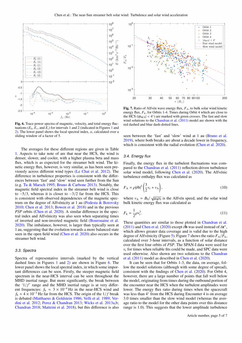
Fig. 6. Trace power spectra of magnetic, velocity, and total energy fluc-tuations (Eb, Ev, and Et) for intervals 1 and 2 (indicated in Figures 1 and2). The lower panel shows the local spectral index, α, calculated over asliding window of a factor of 5.

The averages for these different regions are given in Table1. Aspects to take note of are that near the HCS, the wind isdenser, slower, and cooler, with a higher plasma beta and massflux, which is as expected for the streamer belt wind. The ki-netic energy flux, however, is very similar, as has been seen pre-viously across different wind types (Le Chat et al. 2012). Thedifference in turbulence properties is consistent with the differ-ences between ‘fast’ and ‘slow’ wind seen further from the Sun(e.g. Tu & Marsch 1995; Bruno & Carbone 2013). Notably, themagnetic field spectral index in the streamer belt wind is closeto −5/3, whereas it is closer to −3/2 far from the HCS. Thisis consistent with observed dependencies of the magnetic spec-trum on the degree of Alfvénicity at 1 au (Podesta & Borovsky2010; Chen et al. 2013; Bowen et al. 2018) and in the previousPSP orbits (Chen et al. 2020). A similar difference in the spec-tral index and Alfvénicity was also seen when separating timesof inverted and non-inverted magnetic field (Bourouaine et al.2020). The imbalance, however, is larger than typically seen at1 au, suggesting that the evolution towards a more balanced stateseen in the open field wind (Chen et al. 2020) also occurs in thestreamer belt wind.

3.3. Spectra

Spectra of representative intervals (marked by the verticaldashed lines in Figures 1 and 2) are shown in Figure 6. Thelower panel shows the local spectral index, in which some impor-tant differences can be seen. Firstly, the steeper magnetic fieldspectrum in the near-HCS interval can be seen throughout theMHD inertial range. But more significantly, the break betweenthe ‘1/ f ’ range and the MHD inertial range is at very differ-ent frequencies: fb ≈ 3 × 10−4 Hz in the near-HCS wind andfb ≈ 4 × 10−3 Hz far from the HCS. The origin of the 1/ f breakis debated (Matthaeus & Goldstein 1986; Velli et al. 1989; Ver-dini et al. 2012; Perez & Chandran 2013; Wicks et al. 2013a,b;Chandran 2018; Matteini et al. 2018), but this difference is also

20 30 40 50 60 70 80 90100 200

10-3

10-2

10-1

100

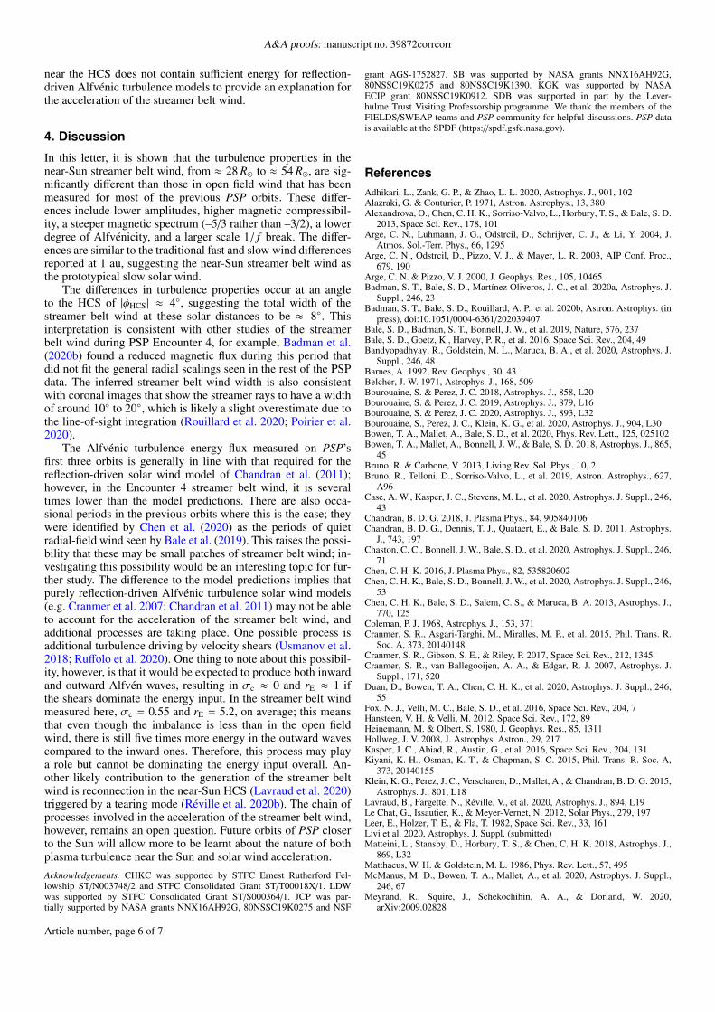
Fig. 7. Ratio of Alfvén wave energy flux, FA, to bulk solar wind kineticenergy flux, Fk, for Orbits 1-4. Times during Orbit 4 which are close tothe HCS (|φHCS| < 4◦) are marked with green crosses. The fast and slowwind solutions to the Chandran et al. (2011) model are shown with thered dashed and blue dash-dotted lines.

seen between the ‘fast’ and ‘slow’ wind at 1 au (Bruno et al.2019), where both breaks are about a decade lower in frequency,which is consistent with the radial evolution (Chen et al. 2020).

3.4. Energy flux

Finally, the energy flux in the turbulent fluctuations was com-pared to the Chandran et al. (2011) reflection-driven turbulencesolar wind model, following Chen et al. (2020). The Alfvénicturbulence enthalpy flux was calculated as

FA = ρ|δb|2(

32

vr + vA

), (10)

where vA = B0/√µ0ρ0 is the Alfvén speed, and the solar wind

bulk kinetic energy flux was calculated as

Fk =12ρv3

r . (11)

These quantities are similar to those plotted in Chandran et al.(2011) and Chen et al. (2020) except δb was used instead of δz+,which allows greater data coverage and is valid due to the highdegree of Alfvénicity (Figure 5). Figure 7 shows the ratio FA/Fk,calculated over 3-hour intervals, as a function of solar distanceover the first four orbits of PSP. The SPAN-I data were used forvr for times when reliable fits could be made, and SPC data wereused otherwise. Also shown are two solutions to the Chandranet al. (2011) model as described in Chen et al. (2020).

It can be seen that for Orbits 1-3, the data, on average, fol-low the model solutions (although with some degree of spread),consistent with the findings of Chen et al. (2020). For Orbit 4,however, there are a large number of points that fall well belowthe model, originating from times during the outbound portion ofthe encounter near the HCS when the turbulent amplitudes werelower. The energy flux ratio during times when the spacecraftwas less than 4◦ from the HCS during Encounter 4 is on average3.0 times smaller than the slow wind model (whereas the aver-age ratio to the model for the other data points over this distancerange is 1.0). This suggests that the lower amplitude turbulence



near the HCS does not contain sufficient energy for reflection-driven Alfvénic turbulence models to provide an explanation forthe acceleration of the streamer belt wind.

4. Discussion

In this letter, it is shown that the turbulence properties in thenear-Sun streamer belt wind, from ≈ 28 R� to ≈ 54 R�, are sig-nificantly different than those in open field wind that has beenmeasured for most of the previous PSP orbits. These differ-ences include lower amplitudes, higher magnetic compressibil-ity, a steeper magnetic spectrum (–5/3 rather than –3/2), a lowerdegree of Alfvénicity, and a larger scale 1/ f break. The differ-ences are similar to the traditional fast and slow wind differencesreported at 1 au, suggesting the near-Sun streamer belt wind asthe prototypical slow solar wind.

The differences in turbulence properties occur at an angleto the HCS of |φHCS| ≈ 4◦, suggesting the total width of thestreamer belt wind at these solar distances to be ≈ 8◦. Thisinterpretation is consistent with other studies of the streamerbelt wind during PSP Encounter 4, for example, Badman et al.(2020b) found a reduced magnetic flux during this period thatdid not fit the general radial scalings seen in the rest of the PSPdata. The inferred streamer belt wind width is also consistentwith coronal images that show the streamer rays to have a widthof around 10◦ to 20◦, which is likely a slight overestimate due tothe line-of-sight integration (Rouillard et al. 2020; Poirier et al.2020).

The Alfvénic turbulence energy flux measured on PSP’sfirst three orbits is generally in line with that required for thereflection-driven solar wind model of Chandran et al. (2011);however, in the Encounter 4 streamer belt wind, it is severaltimes lower than the model predictions. There are also occa-sional periods in the previous orbits where this is the case; theywere identified by Chen et al. (2020) as the periods of quietradial-field wind seen by Bale et al. (2019). This raises the possi-bility that these may be small patches of streamer belt wind; in-vestigating this possibility would be an interesting topic for fur-ther study. The difference to the model predictions implies thatpurely reflection-driven Alfvénic turbulence solar wind models(e.g. Cranmer et al. 2007; Chandran et al. 2011) may not be ableto account for the acceleration of the streamer belt wind, andadditional processes are taking place. One possible process isadditional turbulence driving by velocity shears (Usmanov et al.2018; Ruffolo et al. 2020). One thing to note about this possibil-ity, however, is that it would be expected to produce both inwardand outward Alfvén waves, resulting in σc ≈ 0 and rE ≈ 1 ifthe shears dominate the energy input. In the streamer belt windmeasured here, σc = 0.55 and rE = 5.2, on average; this meansthat even though the imbalance is less than in the open fieldwind, there is still five times more energy in the outward wavescompared to the inward ones. Therefore, this process may playa role but cannot be dominating the energy input overall. An-other likely contribution to the generation of the streamer beltwind is reconnection in the near-Sun HCS (Lavraud et al. 2020)triggered by a tearing mode (Réville et al. 2020b). The chain ofprocesses involved in the acceleration of the streamer belt wind,however, remains an open question. Future orbits of PSP closerto the Sun will allow more to be learnt about the nature of bothplasma turbulence near the Sun and solar wind acceleration.Acknowledgements. CHKC was supported by STFC Ernest Rutherford Fel-lowship ST/N003748/2 and STFC Consolidated Grant ST/T00018X/1. LDWwas supported by STFC Consolidated Grant ST/S000364/1. JCP was par-tially supported by NASA grants NNX16AH92G, 80NSSC19K0275 and NSF

grant AGS-1752827. SB was supported by NASA grants NNX16AH92G,80NSSC19K0275 and 80NSSC19K1390. KGK was supported by NASAECIP grant 80NSSC19K0912. SDB was supported in part by the Lever-hulme Trust Visiting Professorship programme. We thank the members of theFIELDS/SWEAP teams and PSP community for helpful discussions. PSP datais available at the SPDF (https://spdf.gsfc.nasa.gov).

ReferencesAdhikari, L., Zank, G. P., & Zhao, L. L. 2020, Astrophys. J., 901, 102Alazraki, G. & Couturier, P. 1971, Astron. Astrophys., 13, 380Alexandrova, O., Chen, C. H. K., Sorriso-Valvo, L., Horbury, T. S., & Bale, S. D.

2013, Space Sci. Rev., 178, 101Arge, C. N., Luhmann, J. G., Odstrcil, D., Schrijver, C. J., & Li, Y. 2004, J.

Atmos. Sol.-Terr. Phys., 66, 1295Arge, C. N., Odstrcil, D., Pizzo, V. J., & Mayer, L. R. 2003, AIP Conf. Proc.,

679, 190Arge, C. N. & Pizzo, V. J. 2000, J. Geophys. Res., 105, 10465Badman, S. T., Bale, S. D., Martínez Oliveros, J. C., et al. 2020a, Astrophys. J.

Suppl., 246, 23Badman, S. T., Bale, S. D., Rouillard, A. P., et al. 2020b, Astron. Astrophys. (in

press), doi:10.1051/0004-6361/202039407Bale, S. D., Badman, S. T., Bonnell, J. W., et al. 2019, Nature, 576, 237Bale, S. D., Goetz, K., Harvey, P. R., et al. 2016, Space Sci. Rev., 204, 49Bandyopadhyay, R., Goldstein, M. L., Maruca, B. A., et al. 2020, Astrophys. J.

Suppl., 246, 48Barnes, A. 1992, Rev. Geophys., 30, 43Belcher, J. W. 1971, Astrophys. J., 168, 509Bourouaine, S. & Perez, J. C. 2018, Astrophys. J., 858, L20Bourouaine, S. & Perez, J. C. 2019, Astrophys. J., 879, L16Bourouaine, S. & Perez, J. C. 2020, Astrophys. J., 893, L32Bourouaine, S., Perez, J. C., Klein, K. G., et al. 2020, Astrophys. J., 904, L30Bowen, T. A., Mallet, A., Bale, S. D., et al. 2020, Phys. Rev. Lett., 125, 025102Bowen, T. A., Mallet, A., Bonnell, J. W., & Bale, S. D. 2018, Astrophys. J., 865,

45Bruno, R. & Carbone, V. 2013, Living Rev. Sol. Phys., 10, 2Bruno, R., Telloni, D., Sorriso-Valvo, L., et al. 2019, Astron. Astrophys., 627,

A96Case, A. W., Kasper, J. C., Stevens, M. L., et al. 2020, Astrophys. J. Suppl., 246,

43Chandran, B. D. G. 2018, J. Plasma Phys., 84, 905840106Chandran, B. D. G., Dennis, T. J., Quataert, E., & Bale, S. D. 2011, Astrophys.

J., 743, 197Chaston, C. C., Bonnell, J. W., Bale, S. D., et al. 2020, Astrophys. J. Suppl., 246,

71Chen, C. H. K. 2016, J. Plasma Phys., 82, 535820602Chen, C. H. K., Bale, S. D., Bonnell, J. W., et al. 2020, Astrophys. J. Suppl., 246,

53Chen, C. H. K., Bale, S. D., Salem, C. S., & Maruca, B. A. 2013, Astrophys. J.,

770, 125Coleman, P. J. 1968, Astrophys. J., 153, 371Cranmer, S. R., Asgari-Targhi, M., Miralles, M. P., et al. 2015, Phil. Trans. R.

Soc. A, 373, 20140148Cranmer, S. R., Gibson, S. E., & Riley, P. 2017, Space Sci. Rev., 212, 1345Cranmer, S. R., van Ballegooijen, A. A., & Edgar, R. J. 2007, Astrophys. J.

Suppl., 171, 520Duan, D., Bowen, T. A., Chen, C. H. K., et al. 2020, Astrophys. J. Suppl., 246,

55Fox, N. J., Velli, M. C., Bale, S. D., et al. 2016, Space Sci. Rev., 204, 7Hansteen, V. H. & Velli, M. 2012, Space Sci. Rev., 172, 89Heinemann, M. & Olbert, S. 1980, J. Geophys. Res., 85, 1311Hollweg, J. V. 2008, J. Astrophys. Astron., 29, 217Kasper, J. C., Abiad, R., Austin, G., et al. 2016, Space Sci. Rev., 204, 131Kiyani, K. H., Osman, K. T., & Chapman, S. C. 2015, Phil. Trans. R. Soc. A,

373, 20140155Klein, K. G., Perez, J. C., Verscharen, D., Mallet, A., & Chandran, B. D. G. 2015,

Astrophys. J., 801, L18Lavraud, B., Fargette, N., Réville, V., et al. 2020, Astrophys. J., 894, L19Le Chat, G., Issautier, K., & Meyer-Vernet, N. 2012, Solar Phys., 279, 197Leer, E., Holzer, T. E., & Fla, T. 1982, Space Sci. Rev., 33, 161Livi et al. 2020, Astrophys. J. Suppl. (submitted)Matteini, L., Stansby, D., Horbury, T. S., & Chen, C. H. K. 2018, Astrophys. J.,

869, L32Matthaeus, W. H. & Goldstein, M. L. 1986, Phys. Rev. Lett., 57, 495McManus, M. D., Bowen, T. A., Mallet, A., et al. 2020, Astrophys. J. Suppl.,

246, 67Meyrand, R., Squire, J., Schekochihin, A. A., & Dorland, W. 2020,

arXiv:2009.02828



Moncuquet, M., Meyer-Vernet, N., Issautier, K., et al. 2020, Astrophys. J. Suppl.,246, 44

Panasenco, O., Velli, M., D’Amicis, R., et al. 2020, Astrophys. J. Suppl., 246, 54Parashar, T. N., Goldstein, M. L., Maruca, B. A., et al. 2020, Astrophys. J. Suppl.,

246, 58Parker, E. N. 1958, Astrophys. J., 128, 664Parker, E. N. 1965, Space Sci. Rev., 4, 666Perez, J. C., Bourouaine, S., Chen, C. H. K., & Raouafi, N. E. 2020, Astron.

Astrophys. (submitted)Perez, J. C. & Chandran, B. D. G. 2013, Astrophys. J., 776, 124Podesta, J. J. & Borovsky, J. E. 2010, Phys. Plasmas, 17, 112905Poirier, N., Kouloumvakos, A., Rouillard, A. P., et al. 2020, Astrophys. J. Suppl.,

246, 60Réville, V., Velli, M., Panasenco, O., et al. 2020a, Astrophys. J. Suppl., 246, 24Réville, V., Velli, M., Rouillard, A. P., et al. 2020b, Astrophys. J., 895, L20Roberts, D. A., Goldstein, M. L., Matthaeus, W. H., & Ghosh, S. 1992, J. Geo-

phys. Res., 97, 17115Rouillard, A. P., Kouloumvakos, A., Vourlidas, A., et al. 2020, Astrophys. J.

Suppl., 246, 37Ruffolo, D., Matthaeus, W. H., Chhiber, R., et al. 2020, Astrophys. J., 902, 94Shoda, M., Suzuki, T. K., Asgari-Targhi, M., & Yokoyama, T. 2019, Astrophys.

J., 880, L2Szabo, A., Larson, D., Whittlesey, P., et al. 2020, Astrophys. J. Suppl., 246, 47Tu, C.-Y. & Marsch, E. 1995, Space Sci. Rev., 73, 1Usmanov, A. V., Matthaeus, W. H., Goldstein, M. L., & Chhiber, R. 2018, As-

trophys. J., 865, 25van der Holst, B., Sokolov, I. V., Meng, X., et al. 2014, Astrophys. J., 782, 81Velli, M. 1993, Astron. Astrophys., 270, 304Velli, M., Grappin, R., & Mangeney, A. 1989, Phys. Rev. Lett., 63, 1807Verdini, A., Grappin, R., Pinto, R., & Velli, M. 2012, Astrophys. J., 750, L33Verdini, A., Velli, M., Matthaeus, W. H., Oughton, S., & Dmitruk, P. 2010, As-

trophys. J., 708, L116Wicks, R. T., Mallet, A., Horbury, T. S., et al. 2013a, Phys. Rev. Lett., 110,

025003Wicks, R. T., Roberts, D. A., Mallet, A., et al. 2013b, Astrophys. J., 778, 177Woodham, L., Horbury, T. S., Matteini, L., et al. 2020, Astron. Astrophys. (in

press), doi:10.1051/0004-6361/202039415


Documents

solarwind:Turbulenceand solarwind acceleration