SOLAR WIND COMPLEXITY

Iliopoulos A.C., PhD

Democritus University of Thrace

Department of Electrical and Computer Engineering

Xanthi, Greece

The 11th Hellenic Astronomical Conference

8-12 September 2013, Athens

• Microstate

▫ Ion composition and superthermal electrons

▫ Coulomb collisions

▫ Waves and Plasma microinstabilities

▫ Diffusion and Wave-particle interaction

THE SOLAR WIND LABORATORY

• Characteristics

▫ Nonequilibrium thermodynamics

▫ Multicomponent and nuninform

▫ Chaos

▫ Power law scaling

▫ MHD turbulence

▫ Intermittency

▫ Nonextensive statistics

Solar Wind includes ionized and magnetized gas, composed mainly by protons, electrons, alpha particles and heavier ions, continuously flowing away from the solar corona in all directions pervading the interplanetary space.

Solar Wind is a far from equilibrium, chaotic, self similar, multiscale, multifractal and intermittent MHD turbulent system.

e.g. March and Tu, (1997), Burlaga (1993), Carbone et al. (1996), Zelenyi and Milovanov (2004), Macek (2006)

The BMSW instrument (Fast Monitor of the Solar Wind) was specially designed for measuring of solar wind plasma parameters with very high time resolution. The value of ion flux and it’s direction are measured with resolution equal to 31 ms.

The BMSW instrument is installed onboard the high-apogee Spectr-R satellite. This spacecraft was launched on July 18, 2011, into orbit with apogee of ~ 350 000 km, perigee of ~ 50000 km and orbital period of 8.5 days. The BMSW instrument has operated almost permanently since August 6, 2011.

Spectr-R Satellite – BMSW Instrument

Zastenker et al. 2013 (IKI)

Ion Flux (a), density (b), velocity (c), temperature (d) on shock front 26.09.2011

BMSW Data - Solar Wind Parameters

Calm Period Low values, small fluctuations

Shock Period 5 times higher values

Solar wind Ion Flux time series on shock front 26.09.2011 (12:35 UT)

Time Series

N= 604.510 counts

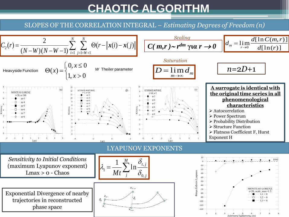
Sensitivity to Initial Conditions (maximum Lyapunov exponent)

Lmax > 0 - Chaos

,

1

0,

1ln

Mt j

j jMt

SLOPES OF THE CORRELATION INTEGRAL – Estimating Degrees of Freedom (n)

Heavyside Function 0, 0

( )1, 0

xx

x

W Theiler parameter

C( m,r ) rdm για r 0 0

[ln ( , )]lim

[ln( )]m

r

d C m rd

d r

n=2D+1

lim mm

D d

2

1 1 1

2( ) ( ( ) ( )

( )( 1)

N N

i j W

C r r i jN W N W

x x

CHAOTIC ALGORITHM

LYAPUNOV EXPONENTS

-2 -1 0 1 2 3 4 5

Ln(r)

0

1

2

3

4

5

6

7

8

Κλίσεις

ΜΟΝΤΕΛΟ LORENZτ=20, w=300

m=3

m=4

m=5

m=6

m=7

m=8

(α)

-4 -2 0 2

Ln(r)

0

1

2

3

4

5

6

7

8

9

10

11

12

13

Κλίσεις

ΛΕΥΚΟΣ ΘΟΡΥΒΟΣτ=1, w=20

m=3

m=4

m=5

m=6

m=7

m=8

m=9

(β)

-5 -4 -3 -2 -1 0 1

Ln(r)

0

1

2

3

4

5

6

7

8

9

10

Κλίσεις

ΕΓΧΡΩΜΟΣ ΘΟΡΥΒΟΣτ=160, w=5

m=3

m=4

m=5

m=6

m=7

m=8

(γ)

1 2 3 4 5 6 7 8 9

Διάσταση Εμβάπτισης (m)

-120

-110

-100

-90

-80

-70

-60

-50

-40

-30

-20

-10

0

10

Φάσμα

Εκθετών

Lya

puno

v

ΜΟΝΤΕΛΟ LORENZτ=20, scale_max=1.5

L1 > 0

L2 = 0

L3 < 0

(στ)

A surrogate is identical with the original time series in all

phenomenological characteristics

Autocorrelation Power Spectrum Probability Distribution Structure Function Flatness Coefficient F, Hurst Exponent H

Exponential Divergence of nearby trajectories in reconstructed

phase space

Scaling

Saturation

Nonequilibrium ( qsen < qstat < qrel) Gaussian-BG equilibrium

(qstat=qsen=qrel=1)

(qstat, qsen, qrel)

(qstat)

TSALLIS q-TRIPLET – Experimental Estimation

12 1[ ] [1 ( 1) ( ) ] q

q qPDF Z A q Z

2ln ( ( ))q i iP z vsz

(qsen)

max min

max min

1sens

a aq

a a

( ) ( 1) qf a qa q D min max( ) ( ) 0f a f a

1lim(log / log )

1

q

q iD p rq

(qrel) 1

relax

sq

s

log ( ) log( )C a s

Multifractal Spectrum Function

Renyi generalized dimension

characterize the attractor set of the dynamics in the phase space of the dynamics

The stationary solutions P(x) describe the probabilistic character of the dynamics on the attractor set of the phase space

The entropy production process is related to the general profile of the attractor set of the dynamics. The profile of the attractor can be described by its multifractality as well as by its sensitivity to initial conditions

Macroscopically, the relaxation to the equilibrium stationary state of some dynamical observable O(t) is related to the evolution of the system in phase space

1ln ( ) ( 1) / (1 )q

q x x q

2

( , ) z

q q

q

G z eC

( )( , ) ( ) ( )i

q q

iq t P t t

( ) ( 1) qq q D

Mass Exponent

TSALLIS q-TRIPLET – Theoretical Estimation

Multifractal Spectrum f(a) – Generalized Dimension D(q)

For the estimation of the multifractal spectrum function we need three parameters (a0, q, X). According to Arimitsu and Arimitsu (2001) we can estimate these parameters by using the equations:

1 1 11 q a a

p - model

2log (1 ) 1q q

qD p p q

The p-model is a one-dimensional model version of a cascade model of eddies. The p-model was introduced to account for the occurrence of intermittency in fully developed turbulence. The best nonlinear fit of the generalized dimension function is represented by

When p = 0.5, then we have a Gaussian Process

21

0 2

( )( ) log [1 (1 ) ] / (1 )

2 ln 2

oa af a D q q

X

1 ( 2)q

( 2)q

2 2

0

(1 )

2 (1 ) (1 ) /

(1 2 ) / [(1 ) ln 2]q

X a q q b

b q

( ) ( 1) qq q D Multifractal Spectrum Function

Intermittency Exponent 2

0 2

2 1( ) 1 [1 log (1 )]

11q

q

Xqq qa C

qC

Calm Period – SOC (Slopes, D = 12 (m=12) – Lyapunov Exponents, Lmax = 0)

Shock Period – CHAOS (Slopes, D = 7.8 (m=12) – Lyapunov Exponents, Lmax > 0)

PHASE TRANSITION

The term ‘‘phase transition process’’ must be understood as a

‘‘metaphase transition’’ process and it is used in order to

characterize the change of the metaequilibrium critical state of the

wind dynamics from the high dimensional solar SOC state to the low

dimensional solar chaos state.

Results – Comparing Calm and Shock Period

Scaling

Saturation

Significant difference

Calm Period – q_stat = 1.38

Shock Period – q_stat = 1.64

Results – Comparing Calm and Shock Period

Strengthening of non-gaussian and Tsallis non-extensive profile

Calm Period – q_sens = - 0.2422 (Singularity Spectrum – Generalized Dimension)

Shock Period – q_sens = 0.2731 (Singularity Spectrum – Generalized Dimension)

Results – Comparing Calm and Shock Period

Intermittency in fully developed

turbulence

Stronger instability and growth of q-entropy production, due to increase of the multifractality

4

2 2

( )

( )

B tF

B t

Results – Studying the Transition

Flatness Coefficient F

4

2 2

( )

( )

B tF

B t

When F = 3, then we have a Gaussian Process

B t B t B t

Increase of long range correlations, non-Gaussian and intermittent character

p – parameter Tsallis entropy

q_sens Multifractal range - Δ(a)

Results – Studying the Transition

Decrease of entropy of the system, self organization, low

complexity level

Timeseries μ * a0 X * q_sen *

Theoretical

q_sen

Experimental

X1 Calm 0.096 1.054±0.001 0.110 -0.251±0.027 -0.2422 ± 0.00009

X2 Calm 0.18 1.103±0.001 0.212 0.224±0.009 0.2713± 0.0024

X3 Calm 0.163 1.093±0.001 0.191 0.160±0.011 0.0904 ± 0.0022

X1 Shock 0.177 1.101±0.001 0.208 0.214±0,010 0.2731 ± 0.0455

X2 Shock 0.255 1.147±0.001 0.303 0.422±0.005 -0.0982 ±0.0031

Results – Studying the Transition

q_stat q_relax

Results – Studying the Transition

Gradual Development of non-Gaussian, non-extensive dynamics

Strengthening of non-Gaussian, non-extensive dynamics (x1 calm vs x1shock)

Large fluctuations

Table 2.

Indices Shock Event

A

Calm

A

Shock

B

Calm

B

Shock

C

Calm

C

Shock

qrel 3.12 3.57 12.89 10.78 8.158 9.772

qstat 1.37 1.52 1.41 1.78 1.38 1.64

qsen 0.0796 0.0217 -0.4384 -0.0071 -0.2422 0.2731

Δα 1.0106 0.9061 0.7023 0.9707 0.7478 1.2045

Δ(Dq) 0.9493 0.8861 0.6661 0.9705 0.6981 1.2106

Tsallis

Entropy

15.47 20.62 199.8 48.05 111 20

Summarizing Results – 3 Shock Events

qstat increases passing from calm to shock period in all cases. However the other two indices changes

depending on the shock event.

Summary of Results

•A phase transition takes place from calm to shock period. In particular, as the estimation of slopes of the correlation dimension and Lyapunov exponent spectrum showed, the calm period corresponds to a self organized critical state while the shock state to a low dimensional chaotic state. • Enhancement of the non-Gaussian character of the dynamics, as the Flatness coefficient F clearly increases to values much higher than 3. • Clear non extensive statistical character of solar wind was observed during the calm or shock periods. • The Tsallis q-triplet parameters increase from calm to shock period. • The multifractal character is strengthened passing from the calm to the shock period, as it is concluded by the profile of singularity spectrum f(α) and the width variation from the calm to the shock state Δ(a). •The parameter p of the p-model estimated from the nonlinear best fitting of the data was found to increase passing from calm to shock period. • Strong reduction of Tsallis entropy production was observed 60-90 minutes before the main shock event. •The intermittency exponent (μ) also increase passing from the calm to shock state. •Faithfull coincidence can be observed between the experimentally estimated singularity spectrum f(α) and the qsen parameter values and the correspondent values estimated using the Tsallis q-entropy principle. •Fluctuations of all parameters were found, a result which indicates the presence of fracton dynamics. • The study of three shock events showed changes in Tsallis q-triplet statistics. Only, the qstat

index increases in all cases. This result needs further investigation.

• Existence of a dynamical non-equilibrium phase transition process related to the solar wind shock event from the original solar wind complex calm state to states which include enhancement of self organization and intermittency.

• Possible precursory phenomena observed minutes before the main shock event.

• The results presented before can be connected with Zelenyi and Milovanov (2004) hypothesis, that the complex character of the solar wind plasma can be described as non-equilibrium (quasi)-stationary states (NESS) having the topology of a percolating fractal set. These scales include multi-scale interactions of fields and particles (currents) and can be related to the simultaneous development of numerous instabilities interfering with each other.

• Finally, the results indicate that the solar wind plasma system can include fracton excitations and fracton dynamics where fracton formations are waves on fractal structures. Fracton dynamics can cause the oscillations of statistical parameters observed during shock events development.

Conclusions

THANK YOU for your attention