SOLAR-HYDROGEN STAND-ALONE POWER SYSTEM

DESIGN AND SIMULATIONS

A THESIS SUBMITTED TO THE GRADUATE SCHOOL OF NATURAL AND APPLIED SCIENCES

OF MIDDLE EAST TECHNICAL UNIVERSITY

BY

ARMAN ULUOĞLU

IN PARTIAL FULFILLMENT OF THE REQUIREMENTS FOR

THE DEGREE OF MASTER OF SCIENCE IN

MECHANICAL ENGINEERING

MAY 2010

Approval of the thesis:

SOLAR-HYDROGEN STAND-ALONE POWER SYSTEM DESIGN AND

SIMULATIONS

submitted by ARMAN ULUOĞLU in partial fulfillment of the requirements for the degree of Master of Science in Mechanical Engineering, Middle East Technical University by,

Prof. Dr. Canan Özgen _______________ Dean, Graduate School of Natural and Applied Sciences Prof. Dr. Suha Oral _______________ Head of Department, Mechanical Engineering Dept., METU

Asst. Prof. Dr. İlker Tarı _______________ Supervisor, Mechanical Engineering Dept., METU Examining Committee Members: Assoc. Prof. Dr. Cemil Yamalı _____________________ Mechanical Engineering Dept., METU Asst. Prof. Dr. İlker Tarı _____________________ Mechanical Engineering Dept., METU Assoc. Prof. Dr. Derek K. Baker _____________________ Mechanical Engineering Dept., METU Asst. Prof. Dr. Tuba Okutucu Özyurt _____________________ Mechanical Engineering Dept., METU Assoc. Prof. Dr. Yüksel Kaplan _____________________ Mechanical Engineering Dept., Niğde University

Date: ______________

iii

I hereby declare that all information in this document has been obtained and presented in accordance with academic rules and ethical conduct. I also declare that, as required by these rules and conduct, I have fully cited and referenced all material and results that are not original to this work.

Name, Last name: Arman Uluoğlu

Signature:

iv

ABSTRACT

SOLAR-HYDROGEN STAND-ALONE POWER SYSTEM DESIGN AND

SIMULATIONS

Uluoğlu, Arman

M.Sc., Department of Mechanical Engineering

Supervisor: Asst. Prof. Dr. İlker Tarı

May 2010, 107 pages

In this thesis, solar-hydrogen Stand-Alone Power System (SAPS) which is planned

to be built for the emergency room of a hospital is designed. The system provides

continuous, off-grid electricity during the whole period of a year without any

external electrical power supply. The system consists of Photovoltaic (PV) panels,

Proton Exchange Membrane (PEM) based electrolyzers, PEM based fuel cells,

hydrogen tanks, batteries, a control mechanism and auxiliary equipments such as

DC/AC converters, water pump, pipes and hydrogen dryers. The aim of this work is

to investigate the optimal system configuration and component sizing which yield

to high performance and low cost for different user needs and control strategies.

TRNSYS commercial software is used for the overall system design and

simulations.

Numerical models of the PV panels, the control mechanism and the PEM

electrolyzers are developed by using theoretical and experimental data and the

models are integrated into TRNSYS. Overall system models include user-defined

components as well as the default software components. The electricity need of

v

the emergency room without any shortage is supplied directly from the PV panels

or by the help of the batteries and the fuel cells when the solar energy is not

enough. The pressure level in the hydrogen tanks and the overall system efficiency

are selected as the key design parameters. The major component parameters and

various control strategies affecting the hydrogen tank pressure and the system

efficiency are analyzed and the results are presented.

Keywords: Stand-Alone Power Systems, TRNSYS, Photovoltaic cells, PEM

electrolyzers, fuel cells, hydrogen.

vi

ÖZ

GÜNEŞ ENERJİSİ VE HİDROJENLİ ŞEBEKEDEN BAĞIMSIZ ENERJİ SİSTEMİ

TASARIMI VE SAYISAL ANALİZİ

Uluoğlu, Arman

Yüksek Lisans, Makina Mühendisliği Bölümü

Tez Yöneticisi: Y. Doç. Dr. İlker Tarı

Mayıs 2010, 107 Sayfa

Bu tezde, bir hastanenin acil servisine kurulması planlanan güneş enerji sistemi

tasarlanmıştır. Bu sistemin tek enerji kaynağı güneş enerjisidir. Sistem tüm yıl

boyunca şebeke elektriğinden yararlanmadan acil servise kesintisiz elektrik enerjisi

sağlar. Güneş enerji sistemi, Fotovoltaik (PV) paneller, PEM bazlı elektrolizörler,

PEM yakıt hücreleri, hidrojen tankı, piller, control mekanizması ve DC/AC

dönüştürücüler, su pompası, borular ve hidrojen kurutucular gibi yan

ekipmanlardan oluşmaktadır. Bu çalışmanın amacı, değişik kullanıcı ihtiyaçlarına ve

control stratejilere göre yüksek performansta ve düşük maliyette çalışacak sistem

konfigürasyonlarını ve ekipman seçimlerini araştırmaktır. Sistemi tümüyle

tasarlamak ve analiz etmek için TRNSYS ticari yazılımı kullanılmıştır. PV

panellerinin, kontrol mekanizmasının ve PEM elektrolizörün sayısal modelleri,

deneysel ve teorik bilgilerden yararlanılarak oluşturulmuş ve TRNSYS yazılımına

eklenmiştir. Tümüyle tasarlanmış system modelleri bu kullanıcı tanımlı elemanlar ve

yazılım içerisinde yer alan varsayılan elemanlar kullanılarak oluşturulmuştur. Acil

servise ihtiyacı olan enerji doğrudan PV panellerinden ya da güneş enerjisi yeterli

olmadığı zamanlar piller ve yakıt hücreleri yardımıyla sürekli ve eksiksiz biçimde

vii

sağlanmaktadır. Hidrojen tankındaki basınç seviyesi ve sistemin toplam verimi

anahtar parametreler olarak seçilmiştir. Bu anahtar parametreleri etkileyen

ekipman seçimleri ve boyutlandırmaları ile control stratejileri incelenmiş ve

sonuçları sunulmuştur.

Anahtar Sözcükler: Şebekeden bağımsız enerji sistemleri, TRNSYS, fotovoltaik

piller, PEM elektrolizörler, yakıt pilleri, hidrojen.

viii

To My Family

ix

ACKNOWLEDGEMENTS

The author wishes to express his deepest gratitude to his supervisor Asst. Prof. Dr.

İlker Tarı for his close guidance, invaluable supervision, encouragements and

insight throughout the study.

I wish to express my sincere appreciation to Prof. Dr. Haluk Aksel for his

understanding and help about using CFD laboratory.

The author would like to thank TUBITAK (project no: Tübitak 106G130) for

supporting this research.

The author would also like to thank his colleague Mr. Ender Özden, for his help and

support throughout the study.

The author gratefully thanks to his family for their continuous encouragement,

understanding and support.

x

TABLE OF CONTENTS

ABSTRACT ………………………………………………………………………………………………… iv

ÖZ …………………………………………………………………………………………………………… vi

ACKNOWLEDGEMENTS ……………………………………………………………………………… ix

TABLE OF CONTENTS ………………………………………………………………………………… x

LIST OF TABLES ………………………………………………………………………………………… xii

LIST OF FIGURES ……………………………………………………………………………………… xiii

LIST OF SYMBOLS ……………………………………………………………………………………… xv

LIST OF ABBREVIATIONS …………………………………………………………………………… xvii

CHAPTERS

1. INTRODUCTION ................................................................................1 

1.1 Renewable Energy........................................................................1 

1.2 Stand Alone Power Systems ..........................................................2 

1.3 TRNSYS .......................................................................................4 

1.4 Literature Survey..........................................................................5 

1.4.1 Experimental Works............................................................5 

1.4.2 Component and System Modeling........................................8 

1.5 Brief Outline...............................................................................11 

2. COMPONENT MODELING..................................................................12 

2.1 Photovoltaic Panel ......................................................................12 

2.1.1 Electrical Model ................................................................13 

2.1.2 Thermal Model .................................................................19 

2.1.3 Maximum Power Point Tracking Model ...............................21 

2.1.4 PV Pane Model Results and Discussion...............................22 

2.2 Proton Exchange Membrane (PEM) Electrolyzer............................27 

2.2.1 Electrolyzer Description.....................................................30 

2.2.2 Electrolyzer Modeling ........................................................31 

3. SYSTEM SIMULATIONS ....................................................................34 

3.1 System Description .....................................................................34 

3.2 Results and Discussions ..............................................................39 

xi

3.2.1 Systems without battery storage .......................................39 

3.2.2 Systems with battery storage ............................................60 

3.2.2 Auxiliary Equipment ..........................................................76 

3.3 TRNSYS Simulations of a Prototype System...........................79 

4. CONCLUSIONS ................................................................................83 

4.1 Results ......................................................................................83 

4.2 Future Work...............................................................................84 

REFERENCES …………………………………………………………………………………………… 86

APPENDICES

A. Data sheet of Kyocera 130W PV panel………………………………………… 90

B. FORTRAN Code of PV Panel Model …………………………………………… 92

C. FORTRAN Code of PEM Electrolyzer Model ………………………………… 96

D. Input files of the system elements……………………………………………… 99

E. Component parameters and experimental models……………………… 105

xii

LIST OF TABLES

TABLES

Table 3-1 PV surface slope and monthly energy production (kWh) ………………… 36

Table 3-2 Description of the energy flows in the system………………………………… 39

Table 3-3 System parameters ……………………………………………………………………… 40

Table 3-4 Component sizes for different systems ………………………………………… 44

Table 3-5 Annual energy flows for different systems (MWh)………………………… 46

Table 3-6 PV surface slope and seasonal energy production ………………………… 57

Table 3-7 Component parameters for different systems ………………………………… 63

Table 3-8 Annual energy flows for different systems (MWh)………………………… 64

Table 3-9 Energy distribution within the system…………………………………………… 81

Table A-1 Electrical specifications………………………………………………………………… 86

Table A-2 Thermal properties……………………………………………………………………… 86

Table E-1 Technical data of the PEM electrolyzer system………………………………… 101

Table E-2 Specification for the PEM fuel cell system……………………………………… 101

xiii

LIST OF FIGURES

FIGURES

Figure 1-1: Stand Alone Power System scheme……………………………………………… 3

Figure 2-1 Equivalent circuit of a solar cell…………………………………………………… 13

Figure 2-2: Cell temperatures for 3 different thermal models………………………… 21

Figure 2-3. Flowchart of Maximum Power Point Tracking………………………………… 22

Figure 2-4. Output power vs. solar irradiation for Kyocera 130……………………… 23

Figure 2-5. PV voltage vs. solar irradiation for Kyocera 130…………………………… 24

Figure 2-6. PV current vs. solar irradiation for Kyocera 130…………………………… 25

Figure 2-7. Output Power of the PV panel with respect to cell temperature …… 26

Figure 2-8. Current-voltage characteristics of the Kyocera 130 PV panel with

respect to cell temperature ………………………………………………………………………… 26

Figure 2-9. Schematics of PEM electrolysis…………………………………………………… 29

Figure 2-10. Voltage-current-temperature characteristic of PEM electrolyzer…… 30

Figure 2-11. Voltage-current-temperature characteristic of PEM electrolyzer…… 32

Figure 3-1. Load profile……………………………………………………………………………… 35

Figure 3-2 TRNSYS schematics of the system………………………………………………… 37

Figure 3-3 Energy flow chart in the system…………………………………………………… 38

Figure 3-4 Power output of PV panels ………………………………………………………… 41

Figure 3-5a Power profile of the components for a summer day …………………… 42

Figure 3-5b Power profile of the components for a winter day ……………………… 43

Figure 3-6 Pressure in the hydrogen tank for system 1…………………………………… 47

Figure 3-7 Power consumed by electrolyzer for system 1……………………………… 48

Figure 3-8 Pressure in the hydrogen tank for system 2…………………………………… 50

Figure 3-9 Cell temperature of the electrolyzer for system 2 ………………………… 51

Figure 3-10 Pressure in hydrogen tank for system 3……………………………………… 53

Figure 3-11 Pressure in hydrogen tank for system 5……………………………………… 55

Figure 3-12 Pressure in hydrogen tank for system 7……………………………………… 56

Figure 3-13 Pressure in hydrogen tank for system 10…………………………………… 59

xiv

Figure 3-14 TRNSYS schematics of the system with battery pack…………………… 62

Figure 3-15 Pressure in hydrogen tank and battery SOC for system 1……………… 66

Figure 3-16 Battery, PV, load and fuel cell power profiles……………………………… 67

Figure 3-17 Annual fuel cell power for system 1…………………………………………… 68

Figure 3-18 Pressure in hydrogen tank and battery SOC for system 3……………… 70

Figure 3-19 Annual fuel cell power for system 3…………………………………………… 71

Figure 3-20 Pressure in hydrogen tank and battery SOC for system 4……………… 73

Figure 3-21 Annual fuel cell power for system 4…………………………………………… 74

Figure 3-22 Pressure in hydrogen tank and battery SOC………………………………… 78

Figure 3-23a Measured battery SOC vs. time………………………………………………… 81

Figure 3-23b Simulated battery SOC vs. time………………………………………………… 81

Figure 3-24a Measured hydrogen SOC vs. time……………………………………………… 82

Figure 3-24b Simulated hydrogen SOC vs. time…………………………………………… 82

Figure A-1 Current-voltage characteristic of PV module KC130TM at various cell

temperatures (adapted from [32])……………………………………………………………… 87

Figure A-2 Current-voltage characteristic of PV module KC130TM at various

irradiance levels (adapted from [32])…………………………………………………………… 87

Figure E-1 Measured current-voltage characteristic at four different electrolyzer

stack-temperatures (adapted from [31]) ……………………………………………………… 102

Figure E-2 Measured current-voltage curves at three different fuel cell stack-

temperatures (adapted from [31]) ……………………………………………………………… 102

Figure E-3 PV power (above) and load (below) profiles emulated by the

programmable power supply used in the experiments (adapted from [31]) …… 103

xv

LIST OF SYMBOLS

Apem PEM surface area

Eg Band gap energy at 0 K

F Faraday constant

I Output current

I0 Reverse saturation current

I0e Exchange current

I0ref Reverse saturation current at Standard Test Conditions

ID Diode current

Iel Electrolyzer current

IL Light current

IPH Photo generated current

Isc,ref Short circuit current at reference conditions

ISH Shunt current

k Boltzmann’s constant

n Diode ideality factor

N Normal conditions (0.101325 MPa and 273.15K)

Ncell Total cell number

ṅh2 Hydrogen molar production rate

Nm3 Volume of the gas calculated at normal conditions which are 273K and 1 Atm in m3

q Elementary charge

R Universal gas constant

RS Series resistance

RSH Shunt resistance

T Absolute cell temperature

xvi

Tc Cell temperature

Tcell,ref Cell temperature at reference conditions

U Cell voltage

Ueq Equilibrium voltage

UPV Convective heat transfer coefficient

V Output voltage

Vt Thermoneutral voltage

w Wind speed m/s

α Absorption coefficient of the cell

αe Symmetry factor

β Temperature coefficient of the PV array

γ Solar irradiance coefficient of the PV array

η PV panel efficiency

ηF Faraday efficiency

ηr Efficiency of the PV array at reference conditions

μIsc Temperature coefficient of short circuit

τ Transmittance of the cell cover

Φ Solar irradiation (mW/cm2)

xvii

LIST OF ABBREVIATIONS

NOCT Nominal Operating Cell Temperature

PEM Proton Exchange Membrane

SAPS Stand Alone Power System

SOC Stane of Charge

STC Standart Test Conditions

TMY Typical Meteorological Year

1 2 CHAPTER 1

INTRODUCTION

1.1 Renewable Energy

As awareness of global warming increases and conventional fuel sources begin to

drain, alternative energy sources attract the attention of the community more and

more every day. Since the political issues decrease the desirability of nuclear

power, a large amount of research and investments focus on renewable energy.

Renewable energy is generated from natural resources like sunlight, wind, hydro,

geothermal energies or from biodiesel fuels. Energy produced from renewable

resources have no major waste products and the resources are naturally

replenished. Although the resources are cost-free and environmentally friendly,

current high initial costs of equipment, low energy conversion efficiencies and

intermittent nature of energy sources decrease economic viability of the renewable

energy against the fossil fuels. However, as the renewable technologies step

forward, the practical use of renewables is growing. During the last decade, many

governments have advanced their support for renewables. According to the

Renewable Energy Policy Network [1] research, 15% of global electricity

production is provided from large hydropower plants and 3.4% from new

renewables (solar, wind, geothermal, biofuels, tidal) in year 2006. In year 2008,

the total investment on new renewable energies has been doubled with respect to

the year 2006 and the total energy production capacity has been increased by

40%. For the majority of analysts, renewable energy industry is a “guaranteed-

growth” sector and even “crisis-proof” because of the worldwide trends and

enormous development in the past decade [2].

1

Solar energy is one of the major sources of renewable energy with the amount of

solar radiation reaching the Earth from the Sun. It is a well known fact that the

world’s one year energy demand can be supplied by the Sun in one hour if it was

possible to collect all the solar energy falling on the earth. There are two

commonly used ways of benefiting from sunlight; solar energy can be used to

produce hot water or air via thermal solar panels or it is possible to convert solar

energy into electricity by photovoltaic (PV) cells. Photovoltaic electricity generation

has various advantages and disadvantages. Main disadvantages are; high initial

cost of the equipment, low efficiency in converting solar energy into electricity and

intermittent energy production due to natural reasons such as no sunlight being

available during the night and low solar radiation throughout the winter seasons.

But, once the PV panels are built, the operation cost of the system is very low and

the panels can work up to 20 years without any special maintenance need. Energy

produced by the PV panels is cost-free and there is not any waste product. With

conventional PV technologies 12 to 18% of solar energy can be converted into

electricity however there are new technologies under development where the

conversion efficiency reaches 40% [3]. Because of the discontinuous energy

production, energy storage or a backup power system is needed for photovoltaic

systems. Batteries can be used for daily storage but for seasonal storage batteries

are not practical because of the low storage capacity. Storing energy in the form of

hydrogen is a possible solution for both daily and seasonal storage.

1.2 Stand Alone Power Systems

A Stand Alone Power System (SAPS) is an off-grid electricity system that can

operate without any external power input. Energy input to the system is usually

from a renewable source. Stand alone power systems are mostly used in remote

locations where transporting electricity is either very difficult or expensive. A

typical solar-hydrogen based stand alone power system, which will be investigated

in this study, with minimum system elements is shown in Figure 1-1 [4]. Main

elements of such systems are the solar energy source, photovoltaic panels,

electrolyzer, fuel-cell and the hydrogen tank. Also some auxiliary equipment is

needed for the system to work properly. The system is controlled by a universal

2

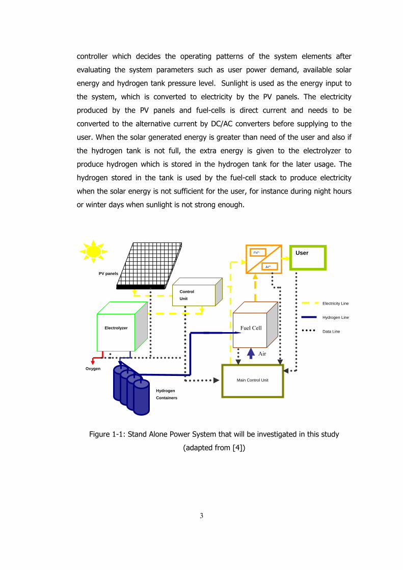
controller which decides the operating patterns of the system elements after

evaluating the system parameters such as user power demand, available solar

energy and hydrogen tank pressure level. Sunlight is used as the energy input to

the system, which is converted to electricity by the PV panels. The electricity

produced by the PV panels and fuel-cells is direct current and needs to be

converted to the alternative current by DC/AC converters before supplying to the

user. When the solar generated energy is greater than need of the user and also if

the hydrogen tank is not full, the extra energy is given to the electrolyzer to

produce hydrogen which is stored in the hydrogen tank for the later usage. The

hydrogen stored in the tank is used by the fuel-cell stack to produce electricity

when the solar energy is not sufficient for the user, for instance during night hours

or winter days when sunlight is not strong enough.

Figure 1-1: Stand Alone Power System that will be investigated in this study

(adapted from [4])

DC

AC

Fuel Cell

Control

Unit

Electrolyzer

Hydrogen

Containers

User

Main Control Unit

Air

Electricity Line

Hydrogen Line

Data Line

PV panels

Oxygen

3

To protect the fuel cell from the harmful effects of switching on and off or

fluctuating operating power, a battery pack can also be installed to the system.

They can be used to help the fuel cell during the peak hours which decreases the

fuel cell power and increases the fuel cell efficiency. Also, batteries can supply

electricity if the user needs very low amount of energy when it is not safe for fuel

cells to operate. Since, the total energy can be stored in batteries is low, they are

not suitable for seasonal storage or daily storage where the user power demand is

high.

It is important to see the behavior of the system before making the final decision

on the singular elements that will be used in the system. To optimize the system

size and quality, it is needed to see how the system works under certain

circumstances, how the system responds to the variations, how efficient the

system is or whether we can supply the demand of the user or not. There are

many commercial software’s available focused on simulating such systems such as

TRNSYS, HOMER and HYBRID2. Also it is possible to simulate these systems by

Matlab, FORTRAN, and other programming languages.

1.3 TRNSYS

During this work TRNSYS (The Transient Energy System Simulation Tool) is used

for the simulations. It is a dynamic simulation program developed in University of

Wisconsin. This tool is one of the most common software for simulations of

thermal energy systems in the literature. The software includes many default

elements that can be used in a stand-alone power system and also it is a flexible

tool that allows any user with a FORTRAN compiler to define their own elements

into the software if necessary. Each component in the software is a FORTRAN

subroutine with input, output and calculation parameters. Every component can be

linked to each other with output/input relations. For instance; a fuel cell

component reads its input such as inlet pressures, physical properties, cell current,

number of cells, cooling data and membrane properties then runs the subroutine

and calculates the output data such as cell voltage, power and temperature,

hydrogen consumption or energy efficiency. By linking the hydrogen consumption

4

output of the fuel cell and hydrogen production output of the electrolyzer to the

hydrogen outflow and hydrogen inflow inputs of the hydrogen tank respectively,

hydrogen tank subroutine can calculate the hydrogen level in the tank. Upon

linking the hydrogen tank output, user power demand and electricity production

output of the PV panels to the system controller, the controller can decide how the

system should work.

TRNSYS has a wide range of use in HVAC applications, hydronics, building projects

and renewable energy systems. Additional component and project libraries can be

added to the software. Simulation periods and time step of simulations are very

flexible and can vary between a second and several years.

1.4 Literature Survey

Stand-Alone Power Systems based on different renewable energies is a developing

topic in the literature. Most of the studies serve as “proof of concept” to using

hydrogen as seasonal energy storage for intermittent renewable energy sources.

The main focus of studies is proving technical viability of this kind of systems.

According to economic point of view, the systems are usually evaluated as not

being feasible with the current prices and efficiencies of the equipments used.

Investment return is usually found to be over 20 years. Detailed knowledge about

renewable energy and system equipment is required to design Stand-Alone Power

Systems. Experimental testing or computational techniques can provide the

necessary information. There are several works in the literature on the design,

operation and simulation processes of renewable energy systems.

1.4.1 Experimental Works

In several studies, performance and viability of renewable energy systems has

been experimentally investigated. Hollmuller et al. [5], Miland and Ulleberg [6],

Vanhanen et al. [7], Galli and Stefanoni [8], Chaparro et al. [9], Sasitharanuwat et

al. [10], Agbossou et al. [11], Shapiro et al. [12] and Kelly et al. [13] have

reported experimental results of prototype or actual systems.

5

Hollmuller et al. [5] studied the performance of a privately owned photovoltaic

hydrogen production and storage installation in a single-family house in

Switzerland. The system is manually controlled. It consists of an array of roof

mounted PV solar panels, a DC–DC converter , an alkaline membrane electrolyzer,

a hydrogen purification unit, a compressor, two metal hydride storage tanks and a

hydrogen operated minibus. The aim of the study is to investigate commercial and

technical viability of using solar energy for seasonal hydrogen storage. It is

observed that using automatic control unit, a hydrogen purification unit that does

not consume hydrogen and larger hydrogen storage via compressed gas cylinders

would increase the system efficiency and performance.

Miland and Ulleberg [6] used a test facility to report the system performance and

operational experience of individual components, subsystems and complete

renewable power systems. To be able to investigate seasonal performance of the

system, PV arrays have been emulated using a programmable power supply unit.

Since a real time testing during a whole year is very time consuming, 7 days with

different solar energy profiles have been selected to investigate seasonal behavior

of the system in a weekly testing. The programmable power supply feeds the

emulated PV power to the system consisting of PEM electrolyzer and fuel cell,

metal hydride tank, hydrogen purifier, control panels and load. The efficiencies of

singular component, subsystems and complete system have been found and ways

to improve them have been proposed. The real time operating efficiency of

system, excluding PV array efficiency, has been found over 50%.

Vanhanen et al. [7] performed an analysis on small scale seasonal energy storage

in the form of hydrogen. Using solid polymer electrolyzers and fuel cells are found

to be more efficient than using alkaline electrolyzers and phosphoric acid fuel cells.

The hydrogen cycle efficiency is around 40-45% and the system is offered to be

viable for small scale stand alone power system which are far away from grid

power.

6

Galli and Stefanoni [8] tested and investigated commercial solar-hydrogen

technologies in a demonstrative solar-hydrogen plant built near Rome. Long term

reliability of solid polymer fuel cell, alkaline electrolyzer and metal hydride and

pressurized storage tank is evaluated. Also the efficiency of storing energy in the

form of hydrogen and the performance losses due to intermittent operation is

investigated. Weather conditions and the performances of PV panels, electrolyzer,

fuel cell and hydrogen tanks are individually monitored.

Chaparro et al. [9] investigated a solar-hydrogen stand alone power system which

supplies 3-5 kWh daily energy throughout a year. The electrolyzer works under

high pressure to avoid hydrogen compression steps but it is found that absorption-

temperature mechanics of metal hydride storage tank is a limiting factor for system

performance. 6-7% of the total solar irradiation is found to be supplied to the user

at the end of the testing year. Hydrogen cycle is reported to be essential because

of the continuous power need, even though the efficiency of this cycle is low.

Sasitharanuwat et al. [10] reported the results of a stand alone power system that

has been built with 3 different types of commercial PV panels in an isolated

building. They system fails to supply continuous energy to the user since a battery

pack was used as the only energy storage. Combining the PV system with a micro-

grid is offered to be as a solution. The excess energy from the PV panels during

day times would be supplied to the micro-grid and during night times electricity

could be drawn from the grid.

Agbossou et al. [11] investigated the performance of a hydrogen stand alone

power system. A wind turbine and PV panels are used together as the energy

generators. Alkaline electrolyzers, PEM fuel cells, hydrogen storage, batteries,

controllers, DC/DC convertors and DC/AC inverters are the other components of

the system. The controller defines the flow path of energy in the system. Batteries

are used to cover energy demand during peak load powers and load power

transients. After 30 days of operation, stand alone power system based on

hydrogen as energy storage is found to be safe and reliable.

7

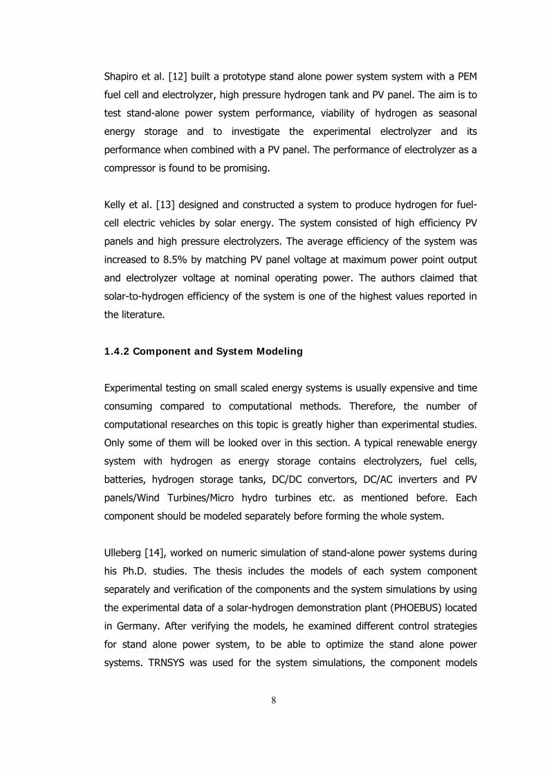
Shapiro et al. [12] built a prototype stand alone power system system with a PEM

fuel cell and electrolyzer, high pressure hydrogen tank and PV panel. The aim is to

test stand-alone power system performance, viability of hydrogen as seasonal

energy storage and to investigate the experimental electrolyzer and its

performance when combined with a PV panel. The performance of electrolyzer as a

compressor is found to be promising.

Kelly et al. [13] designed and constructed a system to produce hydrogen for fuel-

cell electric vehicles by solar energy. The system consisted of high efficiency PV

panels and high pressure electrolyzers. The average efficiency of the system was

increased to 8.5% by matching PV panel voltage at maximum power point output

and electrolyzer voltage at nominal operating power. The authors claimed that

solar-to-hydrogen efficiency of the system is one of the highest values reported in

the literature.

1.4.2 Component and System Modeling

Experimental testing on small scaled energy systems is usually expensive and time

consuming compared to computational methods. Therefore, the number of

computational researches on this topic is greatly higher than experimental studies.

Only some of them will be looked over in this section. A typical renewable energy

system with hydrogen as energy storage contains electrolyzers, fuel cells,

batteries, hydrogen storage tanks, DC/DC convertors, DC/AC inverters and PV

panels/Wind Turbines/Micro hydro turbines etc. as mentioned before. Each

component should be modeled separately before forming the whole system.

Ulleberg [14], worked on numeric simulation of stand-alone power systems during

his Ph.D. studies. The thesis includes the models of each system component

separately and verification of the components and the system simulations by using

the experimental data of a solar-hydrogen demonstration plant (PHOEBUS) located

in Germany. After verifying the models, he examined different control strategies

for stand alone power system, to be able to optimize the stand alone power

systems. TRNSYS was used for the system simulations, the component models

8

were integrated into the software. The current commercial version of TRNSYS also

includes many of these components.

Ulleberg [15] also investigated the control strategy for a PV system with a

hydrogen subsystem using TRNSYS. The investigated system involves an

electrolyzer, a pressurized hydrogen gas storage, and a fuel cell. Detailed

computer simulation models are developed, tested, and verified against a

reference system. The basic control strategy and main logical control variables for

a PV-hydrogen system are described. The results from a time series simulation for

a typical year are presented.

Dufo-Lopez et al. [16] developed a method for controlling stand-alone hybrid

renewable electrical systems with hydrogen storage. The method optimized the

control of the hybrid system by minimizing the total cost throughout its lifetime.

The optimized hybrid system can be composed of renewable sources, batteries,

fuel cell, AC generator and electrolyzer. Also, the control strategy optimizes how

the spare energy is used. The important point of this study is; the control strategy

determines the most economical way to meet the energy deficit, when the amount

of energy demanded by the loads is higher than the one produced by the

renewable sources.

Santarelli et al. [17] investigated a stand-alone energy system supplied just with

renewable energy sources. This system contains an electrolyzer, a hydrogen tank

and a proton exchange membrane fuel cell. The energy systems have been

designed in order to supply the electricity needs of a residential user in a mountain

environment in Italy during a complete year. In this study, three different

renewable sources have been considered : solar irradiance, hydraulic energy and

wind speed.

Pedrazzi et al [18] developed a complete mathematical model for a solar hydrogen

energy system. Each component and subsystem has been modeled separately by

using the information available in the literature. Then the individual models were

combined together to form the virtual system. The simulations were conducted on

9

commercial software MATLAB Simulink. The annual simulations suggested that the

system was able to perform as a stand alone power system without any energy

need from grid. Thermodynamic, exergy and economic analysis’s was planned to

be done by using the reference system modeled.

Samaniego et al. [19] models a hydrogen stand alone power system with wind

turbine using TRNSYS 15 software. The main aim of the study is to investigate the

system performance with respect to 2 different electrolyzer control strategy;

electrolyzer working at constant power or varying power. The default component

models in the software were used to form the system model. The initial cost of the

system is lower with an electrolyzer working at constant power but the system

performance is lower and the system returns the investment in 30 years. Although

the initial cost of the system is higher with second case, the system returns the

investment in 24 years. The investment return is period is found to be excessively

long because of the high equipment cost.

Deshmukh and Boehm [20] modeled individuals components for PV array, wind

turbine, micro-hydro turbine, electrolyzer, fuel cell and compressed hydrogen,

metal hydride and carbon based storages. Electrical and thermal energy

consumption of a typical residential house is also modeled. The authors announced

the physics of equipments such as PV, fuel cell or hydrogen storages are well

understood because of the long investigations and careful attentions on them. But

PEM electrolyzer models were not yet to be very accurate as the number of studies

on them is very limited on the literature as well.

Nelson et al. [21] developed a computer program using MATLAB to evaluate

economics of a hybrid wind/solar hydrogen generation system. The hydrogen

generation system is compared with traditional battery storage. The performances

of both systems were investigated. The authors offered that battery pack is

economically superior to hydrogen as energy storage because of the low efficiency

of fuel cell-electrolyzer hydrogen cycle. But they also added that with the

improvement in fuel cell and electrolyzer technology they can be competitive in the

near future.

10

Onar et al. [22,23] developed a dynamic model for a solar/wind/hydrogen/ultra-

capacitor (UC) energy system using MATLAB Simulink. Wind turbine and PV array

were used to generate input energy to the system, while hydrogen cycle contains

electrolyzer and fuel cells. UC was set to meet the load demand above maximum

power of fuel cell. The components and subsystems are modeled separately.

Dynamic responses of the components to load, solar irradiation and wind speed

changes are investigated and found to be efficient.

1.5 Brief Outline

In the following chapter, PV panel and electrolyzer are mathematically modeled

and the model performances are discussed. In Chapter 3, the effects of different

system parameters such as PV panel size and surface slope, electrolyzer size,

hydrogen tank capacity, auxiliary equipment, battery pack energy capacity and

operation strategies of batteries on the system performance are analyzed. First,

different stand alone power system configurations without battery pack are

simulated and the results are discussed. Then, detailed analysis on stand alone

power systems with battery pack is discussed and energy consumption of auxiliary

equipment is briefly discussed. TRNSYS simulation of a small scale actual system is

conducted in the last part of Chapter 3. In the last chapter, the results are

discussed, some conclusions are drawn and the future work is suggested.

11

3 4 CHAPTER 2

COMPONENT MODELING

Various components of the solar-hydrogen energy system and related modeling

approaches are presented in this chapter.

2.1 Photovoltaic Panel

A photovoltaic panel is an assembly of PV cells which are semi-conductor materials

generating electricity from electro-magnetic radiation. When the source of

radiation is the Sun, the PV cells are called solar cells. Most of the commercial solar

panels are produced from silicon based solar cells. According to the quality of the

cell, the energy conversion efficiency of the devices from solar power into direct

current can be in the range of 5% to 20%. Because of the low energy conversion

efficiencies and high cost of the solar panels, practical use of these devices are

mostly limited to electricity generation in rural and remote areas, to

telecommunication stations and to spacecrafts.

In the following sub-sections, a mathematical model of solar panels will be

introduced. The model will be able to predict the output parameters of the PV

panel such as power production, cell temperature and efficiency for a given set of

meteorological data. In addition, it will be possible to measure the different

commercial panel performances in generating electricity by changing the input

data provided by producers. In order to use this PV model in the software TRNSYS

which is used to model the complete energy system, the code of the model is

written in FORTRAN programming language.

12

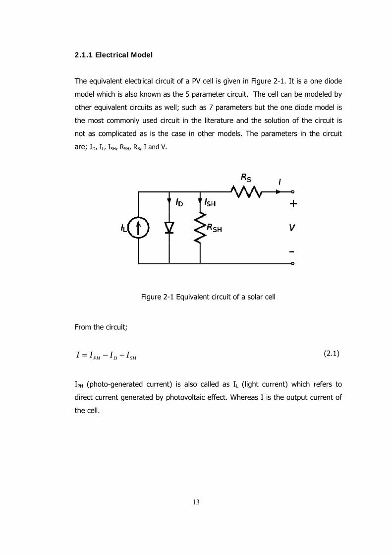
2.1.1 Electrical Model

The equivalent electrical circuit of a PV cell is given in Figure 2-1. It is a one diode

model which is also known as the 5 parameter circuit. The cell can be modeled by

other equivalent circuits as well; such as 7 parameters but the one diode model is

the most commonly used circuit in the literature and the solution of the circuit is

not as complicated as is the case in other models. The parameters in the circuit

are; ID, IL, ISH, RSH, RS, I and V.

Figure 2-1 Equivalent circuit of a solar cell

From the circuit;

PH D SHI I I I (2.1)

IPH (photo-generated current) is also called as IL (light current) which refers to

direct current generated by photovoltaic effect. Whereas I is the output current of

the cell.

13

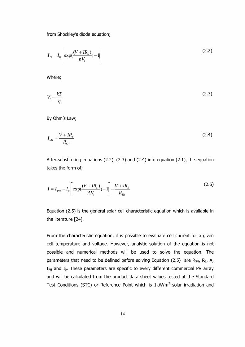
from Shockley’s diode equation;

0

( )exp( ) 1S

Dt

V IRI I

nV

(2.2)

Where;

t

kTV

q

(2.3)

By Ohm’s Law;

SSH

SH

V IRI

R

(2.4)

After substituting equations (2.2), (2.3) and (2.4) into equation (2.1), the equation

takes the form of;

0

( )exp( ) 1S S

PHt SH

V IR V IRI I I

AV R

(2.5)

Equation (2.5) is the general solar cell characteristic equation which is available in

the literature [24].

From the characteristic equation, it is possible to evaluate cell current for a given

cell temperature and voltage. However, analytic solution of the equation is not

possible and numerical methods will be used to solve the equation. The

parameters that need to be defined before solving Equation (2.5) are RSH, RS, A,

IPH and I0. These parameters are specific to every different commercial PV array

and will be calculated from the product data sheet values tested at the Standard

Test Conditions (STC) or Reference Point which is 1kW/m2 solar irradiation and

14

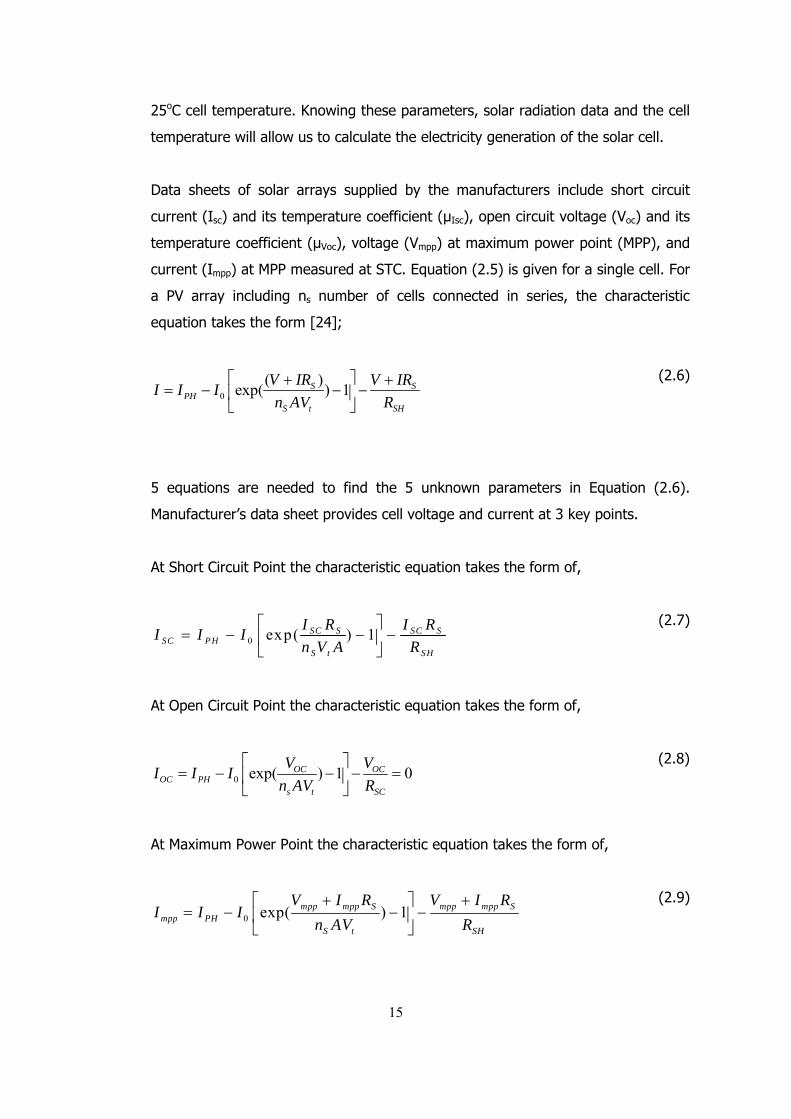
25oC cell temperature. Knowing these parameters, solar radiation data and the cell

temperature will allow us to calculate the electricity generation of the solar cell.

Data sheets of solar arrays supplied by the manufacturers include short circuit

current (Isc) and its temperature coefficient (μIsc), open circuit voltage (Voc) and its

temperature coefficient (μVoc), voltage (Vmpp) at maximum power point (MPP), and

current (Impp) at MPP measured at STC. Equation (2.5) is given for a single cell. For

a PV array including ns number of cells connected in series, the characteristic

equation takes the form [24];

0

( )exp( ) 1S S

PHS t SH

V IR V IRI I I

n AV R

(2.6)

5 equations are needed to find the 5 unknown parameters in Equation (2.6).

Manufacturer’s data sheet provides cell voltage and current at 3 key points.

At Short Circuit Point the characteristic equation takes the form of,

0 exp( ) 1SC S SC SSC PH

S t SH

I R I RI I I

n V A R

(2.7)

At Open Circuit Point the characteristic equation takes the form of,

0 exp( ) 1 0OC OCOC PH

s t SC

V VI I I

n AV R

(2.8)

At Maximum Power Point the characteristic equation takes the form of,

0 exp( ) 1mpp mpp S mpp mpp Smpp PH

S t SH

V I R V I RI I I

n AV R

(2.9)

15

Derivative of the power with respect to voltage at the maximum power point is

equal to zero by the definition of the maximum power point.

0 exp( ) 1( )

0

mpp mpp S mpp mpp SPH mpp

S t SH

V I R V I Rd I I V

n AV RdP d IV

dV dV dV

(2.10)

At 3 key points, there are 4 equations written. There should be 1 more equation to

extract the 5 unknown parameters. Since the series resistance is relatively small

with respect to shunt resistance, IL can be assumed to be equal to ISH Ulleberg

[14].

L SCI I

(2.11)

When equation (2.11) is integrated into previous 4 equations, the number of

unknown parameters decreases to 4. To solve the 4 non-linear equations with 4

unknowns, modified Newton-Raphson method is used. In this method, by using

the derivatives of the equations, non-linear equations are linearized and linear set

of equations can be solved with Gauss elimination method.

Reorganizing the equations (2.7), (2.8), (2.9) and (2.10) respectively;

01 0 exp( ) 1SC S SC SPH SC

S t SH

I R I Rf I I I

n V A R

(2.12)

02 0 exp( ) 1OC OCPH

s t SC

V Vf I I

n AV R

(2.13)

03 0 exp( ) 1 Impp mpp S mpp mpp SPH mpp

S t SH

V I R V I Rf I I

n AV R

(2.14)

16

0 exp( ) 1( )

4 0

mpp mpp S mpp mpp SPH mpp

S t SH

V I R V I Rd I I V

n AV Rd IVf

dV dV

(2.15)

Expanding the solution format given for single equation single unknown to multiple

variable case yields the following set of equations;

There are 4 linear equations with 4 unknowns,

This set of linear equations is solved by Gauss elimination method for the

unknowns. With forward elimination the 4x4 matrix is reduced into upper-triangle

matrix and with backward substitution unknown parameters are calculated. The

code starts from the 4 non-linear equations with initial estimation for the unknown

parameters and replaces them with calculated ones after the backward

1 1 10 1 00 0

1 1 1 1 1 1 1 11

i i i i i i

i i i i i i i iS sh i i S sh i

S sh S sh

f f f f f f f fR R I A f R R I A

R R I A R R I A

1 1 10 1 00 0

2 2 2 2 2 2 2 22

i i i i i i

i i i i i i i iS sh i i S sh i

S sh S sh

f f f f f f f fR R I A f R R I A

R R I A R R I A

1 1 10 1 00 0

3 3 3 3 3 3 3 33

i i i i i i

i i i i i i i iS sh i i S sh i

S sh S sh

f f f f f f f fR R I A f R R I A

R R I A R R I A

1 1 10 1 00 0

4 4 4 4 4 4 4 44

i i i i i i

i i i i i i i iS sh i i S sh i

S sh S sh

f f f f f f f fR R I A f R R I A

R R I A R R I A

1 1 1

1 1 1

1 1 1

1 1 1

1 1 1 0 1 1

2 2 2 0 2 1

3 3 3 0 3 1

4 4 4 0 4 1

. . . .

. . . .

. . . .

. . . .

i i i

i i i

i i i

i i i

S sh i

S sh i

S sh i

S sh i

a R b R c I d A j

a R b R c I d A k

a R b R c I d A l

a R b R c I d A m

17

substitution. The iteration is repeated until the desired value of convergence is

reached. The convergence of Newton-Raphson method highly depends on the

initial guesses of the unknowns and the nature of the functions. With good

knowledge of the parameters in the electrical model of a PV cell, the initial guesses

should be predicated to increase the effectiveness of the method. There are some

cases where this method performs poorly such as; multiple roots or zero slope of a

function.

The parameters evaluated after the iterative process are valid for STC; but the cell

temperature affects these parameters. There are numerous different models for I0

and IPH in the literature. One of the commonly used temperature dependency of

the parameters is given below by Vachtsevanos and Kalaitzakis [25]. Total solar

radiation on the PV surface (Φ) is read by the panel model from the meteorological

data for a given location.

30 0

, ,

1 1( ) exp ( )gcell

refcell ref cell ref cell

qETI I

T kA T T

(2.16)

, , )(1000PH sc ref Isc cell cell refI I T T

(2.17)

The temperature dependency of the parameters RSH, RS and A are given in

Deshmukh and Boehm [20].

ref

pvref

pv

TA A

T

(2.18)

ref

ref

pv

sh shpv

R R

(2.19)

re fS SR R (2.20)

18

2.1.2 Thermal Model

The performance of the PV array is significantly affected by the cell temperature.

The experiments conducted by Mattei et al. [26] show that the output power of

the array decreases from 0.3% up to 0.6% per oC increase in the cell temperature.

Mattei et al. [26] investigate the thermal models of PV cells in the literature,

compares their accuracy and offers their own model. One of the common models

for calculating cell temperatures given in equation (2.21) by using the Nominal

Operating Cell Temperature (NOCT), measured at w=1 m/s wind speed, Ta=20oC

ambient temperature and Φ=800W/m2 solar radiation.

( 20 )800

oc aT T NOCT C

(2.21)

The experiments by Mattei et al. show that this model functions adequately under

certain circumstances. However, since the effect of wind speed is not included into

the model, it does not yield satisfying results under windy environmental

conditions.

Another common thermal model, using absorption coefficient ( ) and

transmittance of the cell cover ( ), is in the form of equation (2.22)

( )PV c aU T T

(2.22)

and the most known cell efficiency equation is given below;

1 ( )r c rT T Log

(2.23)

Combining equations (2.22) and (2.23)

19

( )PV a r r rc

PV r

U T TT

U

(2.24)

Mattei et al. studied the results of many other authors using the same thermal

balance equation but using different convective heat transfer coefficients and they

offer a heat transfer coefficient given in Equation (2.25).

2o24.1 2.9 (W / m C)PVU w (2.25)

A simple TRNSYS software simulation is made to examine and to compare with the

default 5-parameter PV array model developed by Beckman et al. [27] in the

software.

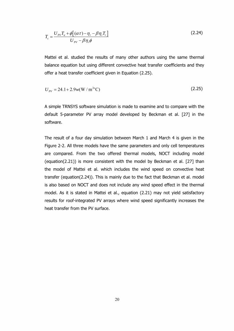
The result of a four day simulation between March 1 and March 4 is given in the

Figure 2-2. All three models have the same parameters and only cell temperatures

are compared. From the two offered thermal models, NOCT including model

(equation(2.21)) is more consistent with the model by Beckman et al. [27] than

the model of Mattei et al. which includes the wind speed on convective heat

transfer (equation(2.24)). This is mainly due to the fact that Beckman et al. model

is also based on NOCT and does not include any wind speed effect in the thermal

model. As it is stated in Mattei et al., equation (2.21) may not yield satisfactory

results for roof-integrated PV arrays where wind speed significantly increases the

heat transfer from the PV surface.

20

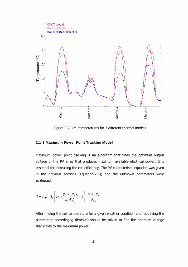
Figure 2-2: Cell temperatures for 3 different thermal models

2.1.3 Maximum Power Point Tracking Model

Maximum power point tracking is an algorithm that finds the optimum output

voltage of the PV array that produces maximum available electrical power. It is

essential for increasing the cell efficiency. The PV characteristic equation was given

in the previous sections (Equation(2.6)) and the unknown parameters were

evaluated.

0

( )exp( ) 1S S

PHS t SH

V IR V IRI I I

n AV R

After finding the cell temperature for a given weather condition and modifying the

parameters accordingly; dP/dV=0 should be solved to find the optimum voltage

that yields to the maximum power.

-NOCT model -Model of Mattei et al. -Model of Beckman et al.

Mar

ch 4

Mar

ch 3

Mar

ch 2

Mar

ch 1

40

31

22

4

-5

Tem

pera

ture

(o C

)

13

21

( )0

dP d IV dII V

dV dV dV

(2.26)

Solution algorithm for the MPPT is given in Figure 2-3. For the initial estimation of

cell voltage, the cell current is evaluated from the characteristic equation then the

derivative of cell power with respect to the voltage is calculated. If the derivative is

lesser than zero, the cell voltage is larger than the optimum value and the

calculations are repeated after the cell voltage is reduced by the defined step size.

If the derivative is larger than zero, the cell voltage is lesser than the optimum

value and the calculations are repeated after the cell voltage is increased by a

defined step size. The process is repeated until the derivative of cell power with

respect to voltage reaches 0.

Figure 2-3. Flowchart of Maximum Power Point Tracking

2.1.4 PV Panel Model Results and Discussion

The model performance is compared with the experimental data of Kyocera 130W

panels collected in Hidronerji building in Ostim/ANKARA. Manufacturer’s data sheet

of the panel is given in Appendix A. Fortran codes of the PV panel model are given

Initial V

Find I from Eq’n (2.6)

Check dP/dV from Eq’n (2.26)

dP/dV= 0

Pmax= Vnew * Inew

dP/dV>0 dP/dV<0

Vnew=Vold+h Vnew=Vold-h

22

in Appendix B. Manufacturer’s data sheet parameters, total radiation on the PV

surface, the ambient temperature and the wind speed are the input of the model.

Then, the model evaluates the output power, the voltage and current, the energy

efficiency and the cell temperature.

PV power vs. Total solar irradiation

0

50

100

150

200

250

300

350

400

0 100 200 300 400 500 600 700 800

Solar irradiation (W/m2)

Po

wer

(W

)

Experimental DataAmbient T=20 CAmbient T=15 CAmbient T=0 C

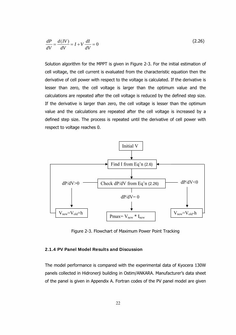
Figure 2-4 Output power vs. solar irradiation for Kyocera 130W

Figure 2-4 shows the comparison between the measured output power and output

power of the numerical model with respect to total solar irradiation. There are 4 PV

panels in Hidronerji. The connection setup of the PV panels is 2 in series and 2 in

parallel. The output current and voltage are both doubled by this configuration.

The data collected by Hidronerji does not include the thermal data such as ambient

temperature, the wind speed and the cell temperature; therefore the experimental

medium cannot be fully projected on the numerical analysis. Three different

ambient temperatures are used during the simulation of the mathematical model.

Variations in cell temperature and angle between the sun and the PV panels are

the possible reasons of the variations in PV power between 450 W and 550 W total

solar irradiation. Output voltage and current comparisons of the numerical model

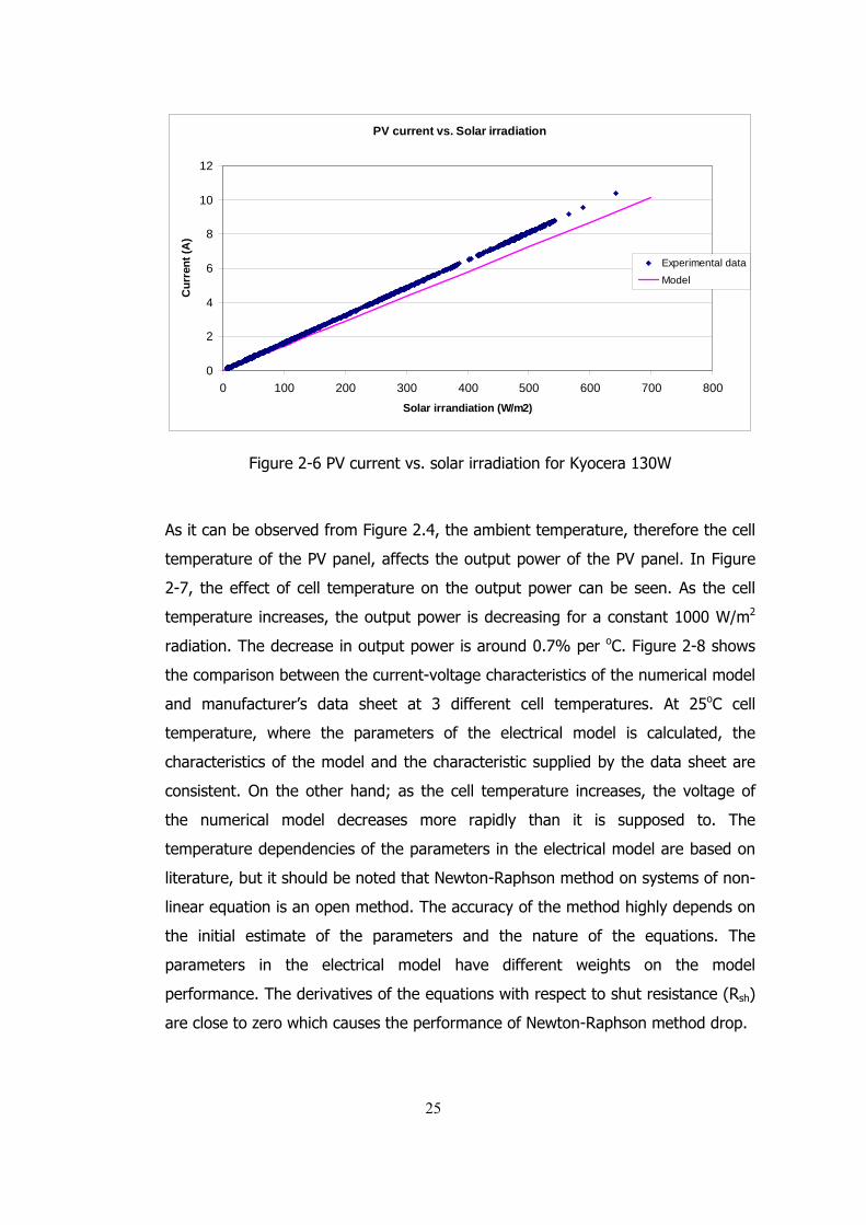
23

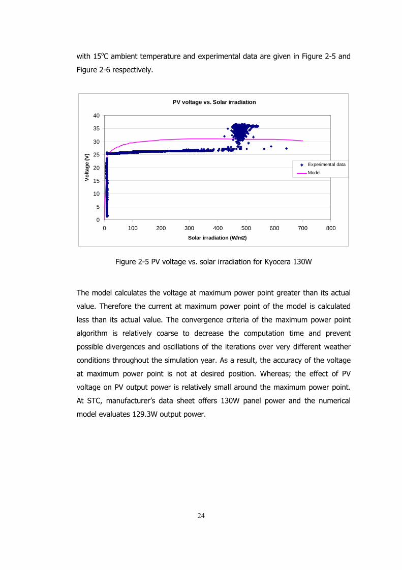
with 15oC ambient temperature and experimental data are given in Figure 2-5 and

Figure 2-6 respectively.

PV voltage vs. Solar irradiation

0

5

10

15

20

25

30

35

40

0 100 200 300 400 500 600 700 800

Solar irradiation (W/m2)

Vo

ltag

e (V

)

Experimental data

Model

Figure 2-5 PV voltage vs. solar irradiation for Kyocera 130W

The model calculates the voltage at maximum power point greater than its actual

value. Therefore the current at maximum power point of the model is calculated

less than its actual value. The convergence criteria of the maximum power point

algorithm is relatively coarse to decrease the computation time and prevent

possible divergences and oscillations of the iterations over very different weather

conditions throughout the simulation year. As a result, the accuracy of the voltage

at maximum power point is not at desired position. Whereas; the effect of PV

voltage on PV output power is relatively small around the maximum power point.

At STC, manufacturer’s data sheet offers 130W panel power and the numerical

model evaluates 129.3W output power.

24

PV current vs. Solar irradiation

0

2

4

6

8

10

12

0 100 200 300 400 500 600 700 800

Solar irrandiation (W/m2)

Cu

rren

t (A

)

Experimental data

Model

Figure 2-6 PV current vs. solar irradiation for Kyocera 130W

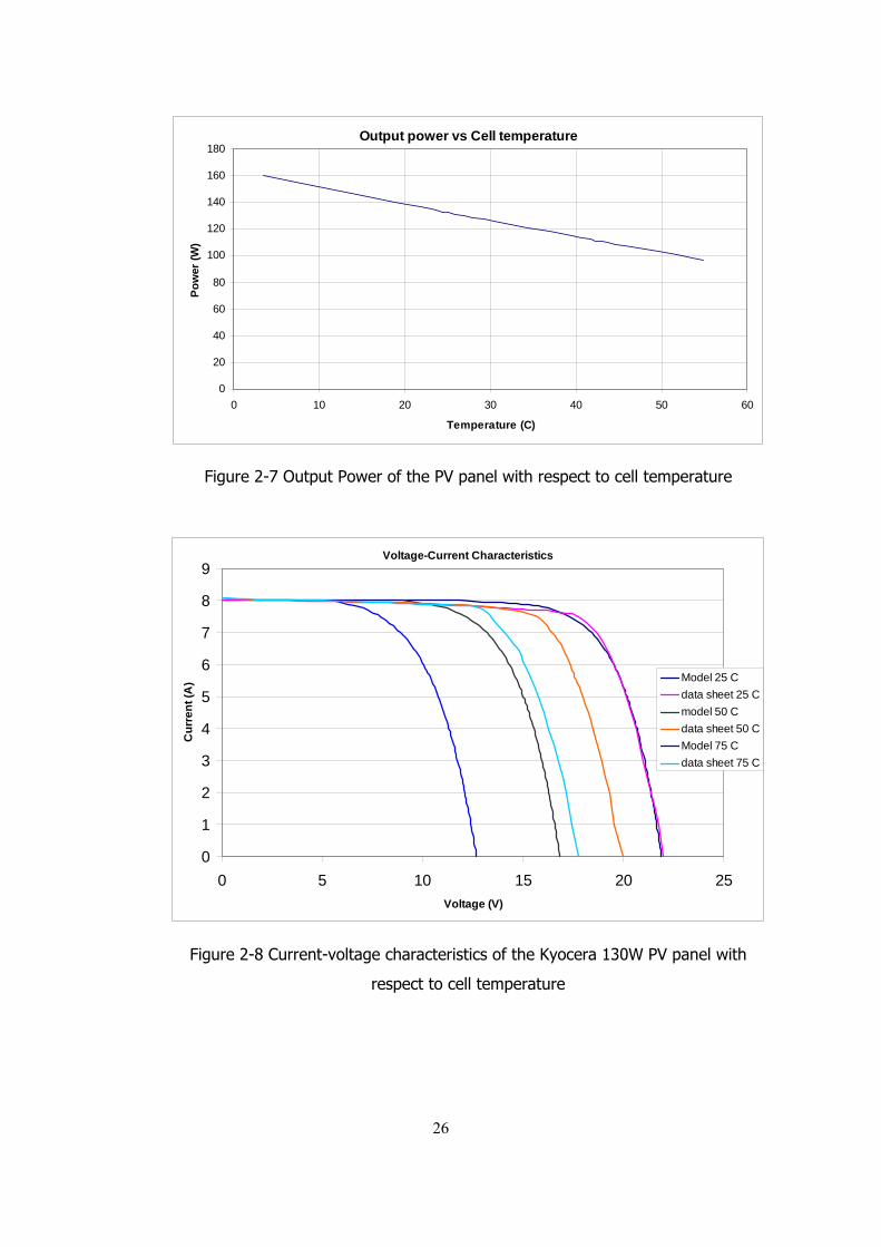
As it can be observed from Figure 2.4, the ambient temperature, therefore the cell

temperature of the PV panel, affects the output power of the PV panel. In Figure

2-7, the effect of cell temperature on the output power can be seen. As the cell

temperature increases, the output power is decreasing for a constant 1000 W/m2

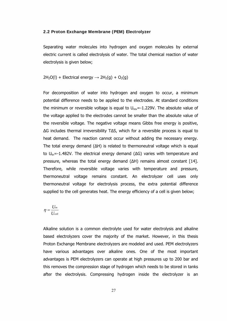
radiation. The decrease in output power is around 0.7% per oC. Figure 2-8 shows

the comparison between the current-voltage characteristics of the numerical model

and manufacturer’s data sheet at 3 different cell temperatures. At 25oC cell

temperature, where the parameters of the electrical model is calculated, the

characteristics of the model and the characteristic supplied by the data sheet are

consistent. On the other hand; as the cell temperature increases, the voltage of

the numerical model decreases more rapidly than it is supposed to. The

temperature dependencies of the parameters in the electrical model are based on

literature, but it should be noted that Newton-Raphson method on systems of non-

linear equation is an open method. The accuracy of the method highly depends on

the initial estimate of the parameters and the nature of the equations. The

parameters in the electrical model have different weights on the model

performance. The derivatives of the equations with respect to shut resistance (Rsh)

are close to zero which causes the performance of Newton-Raphson method drop.

25

Output power vs Cell temperature

0

20

40

60

80

100

120

140

160

180

0 10 20 30 40 50 60

Temperature (C)

Po

wer

(W

)

Figure 2-7 Output Power of the PV panel with respect to cell temperature

Voltage-Current Characteristics

0

1

2

3

4

5

6

7

8

9

0 5 10 15 20 25

Voltage (V)

Cu

rre

nt

(A) Model 25 C

data sheet 25 C

model 50 C

data sheet 50 C

Model 75 C

data sheet 75 C

Figure 2-8 Current-voltage characteristics of the Kyocera 130W PV panel with

respect to cell temperature

26

2.2 Proton Exchange Membrane (PEM) Electrolyzer

Separating water molecules into hydrogen and oxygen molecules by external

electric current is called electrolysis of water. The total chemical reaction of water

electrolysis is given below;

2H2O(l) + Electrical energy → 2H2(g) + O2(g)

For decomposition of water into hydrogen and oxygen to occur, a minimum

potential difference needs to be applied to the electrodes. At standard conditions

the minimum or reversible voltage is equal to Urev=-1.229V. The absolute value of

the voltage applied to the electrodes cannot be smaller than the absolute value of

the reversible voltage. The negative voltage means Gibbs free energy is positive,

ΔG includes thermal irreversibility TΔS, which for a reversible process is equal to

heat demand. The reaction cannot occur without adding the necessary energy.

The total energy demand (ΔH) is related to thermoneutral voltage which is equal

to Utn=-1.482V. The electrical energy demand (ΔG) varies with temperature and

pressure, whereas the total energy demand (ΔH) remains almost constant [14].

Therefore, while reversible voltage varies with temperature and pressure,

thermoneutral voltage remains constant. An electrolyzer cell uses only

thermoneutral voltage for electrolysis process, the extra potential difference

supplied to the cell generates heat. The energy efficiency of a cell is given below;

tn

cell

U

U

Alkaline solution is a common electrolyte used for water electrolysis and alkaline

based electrolyzers cover the majority of the market. However, in this thesis

Proton Exchange Membrane electrolyzers are modeled and used. PEM electrolyzers

have various advantages over alkaline ones. One of the most important

advantages is PEM electrolyzers can operate at high pressures up to 200 bar and

this removes the compression stage of hydrogen which needs to be stored in tanks

after the electrolysis. Compressing hydrogen inside the electrolyzer is an

27

isothermal process which is the most efficient way to compress hydrogen. PEM

electrolyzers have less parasitic losses and higher efficiency than alkaline

electrolyzers which also decreases the cost of hydrogen production.

In addition, highly pure hydrogen can be produced with a long life time by PEM

electrolyzers. Since there is no chemical electrolyte such as KOH used, they are

ecologically clean. Moreover, PEM electrolyzers have smaller sizes and mass

because of the simple and compact design. On the other hand, there are also

some disadvantages; high initial cost of equipment like the membrane cost and

special alloys for the casings, pure water needs to be supplied, low efficiency at

high pressures because of hydrogen permeation and safety issues at low loads in

case of hydrogen mixing with oxygen. Since PEM fuel cells and electrolyzers use

similar materials and have similar design, they have improving technology parallel

to fuel cells.

The schematics of PEM electrolysis is given in Figure 2-9. Water molecules are split

into oxygen and hydrogen at the anode by direct voltage which needs to be higher

than thermoneutral voltage. Hydrogen atoms pass through the proton exchange

membrane and forms hydrogen molecules at the cathode. The proton exchange

membrane is a porous medium which only lets hydrogen atoms pass through. The

electrodes are also porous and the flow fields are between electrodes and end

plates.

28

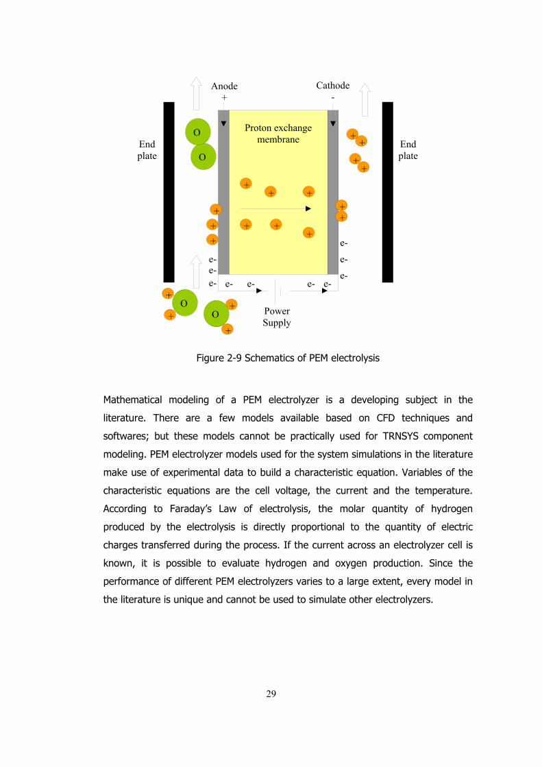
Figure 2-9 Schematics of PEM electrolysis

Mathematical modeling of a PEM electrolyzer is a developing subject in the

literature. There are a few models available based on CFD techniques and

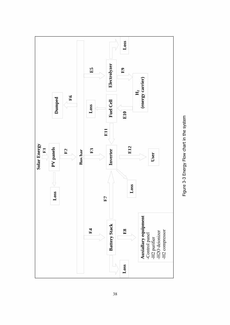
softwares; but these models cannot be practically used for TRNSYS component

modeling. PEM electrolyzer models used for the system simulations in the literature

make use of experimental data to build a characteristic equation. Variables of the

characteristic equations are the cell voltage, the current and the temperature.

According to Faraday’s Law of electrolysis, the molar quantity of hydrogen

produced by the electrolysis is directly proportional to the quantity of electric

charges transferred during the process. If the current across an electrolyzer cell is

known, it is possible to evaluate hydrogen and oxygen production. Since the

performance of different PEM electrolyzers varies to a large extent, every model in

the literature is unique and cannot be used to simulate other electrolyzers.

Anode +

Cathode -

Proton exchange membrane

+O

O

O

O

+

+

+

+ ++

++ +

+

+

+ ++

++

++

e- e- e- e- e- e- e-

e-

e-

e-

Power Supply

End plate

End plate

29

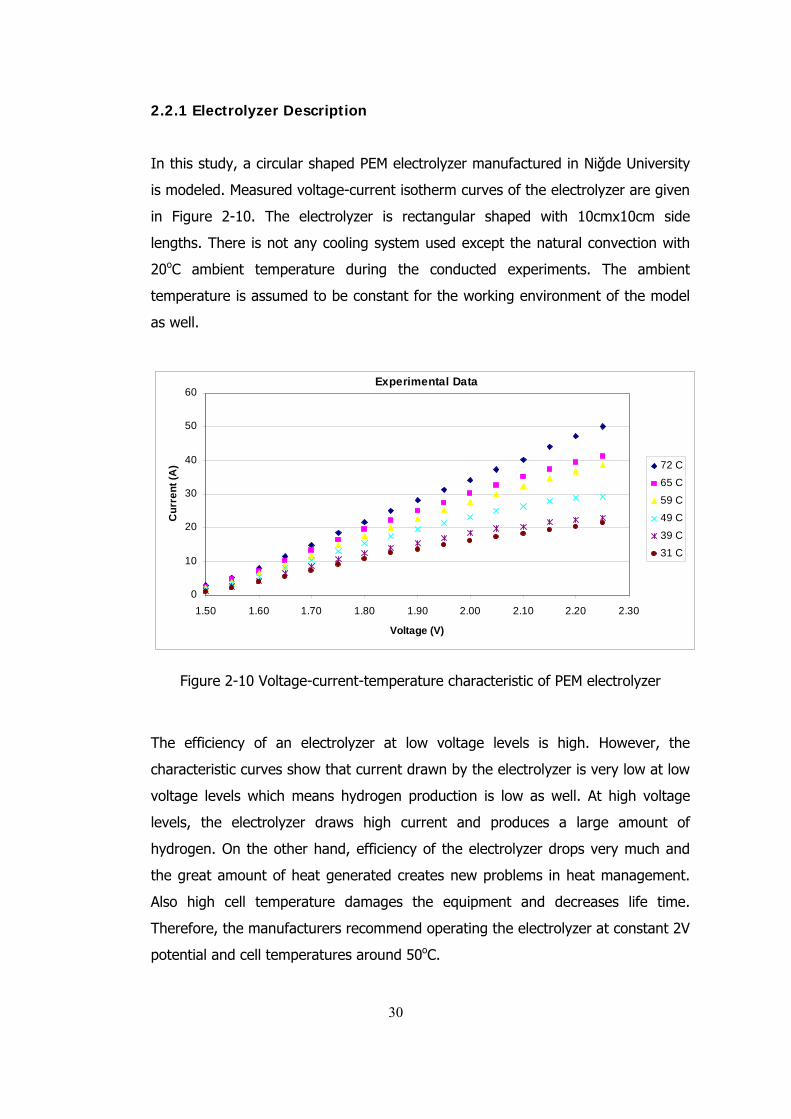
2.2.1 Electrolyzer Description

In this study, a circular shaped PEM electrolyzer manufactured in Niğde University

is modeled. Measured voltage-current isotherm curves of the electrolyzer are given

in Figure 2-10. The electrolyzer is rectangular shaped with 10cmx10cm side

lengths. There is not any cooling system used except the natural convection with

20oC ambient temperature during the conducted experiments. The ambient

temperature is assumed to be constant for the working environment of the model

as well.

Experimental Data

0

10

20

30

40

50

60

1.50 1.60 1.70 1.80 1.90 2.00 2.10 2.20 2.30

Voltage (V)

Cu

rre

nt

(A) 72 C

65 C

59 C

49 C

39 C

31 C

Figure 2-10 Voltage-current-temperature characteristic of PEM electrolyzer

The efficiency of an electrolyzer at low voltage levels is high. However, the

characteristic curves show that current drawn by the electrolyzer is very low at low

voltage levels which means hydrogen production is low as well. At high voltage

levels, the electrolyzer draws high current and produces a large amount of

hydrogen. On the other hand, efficiency of the electrolyzer drops very much and

the great amount of heat generated creates new problems in heat management.

Also high cell temperature damages the equipment and decreases life time.

Therefore, the manufacturers recommend operating the electrolyzer at constant 2V

potential and cell temperatures around 50oC.

30

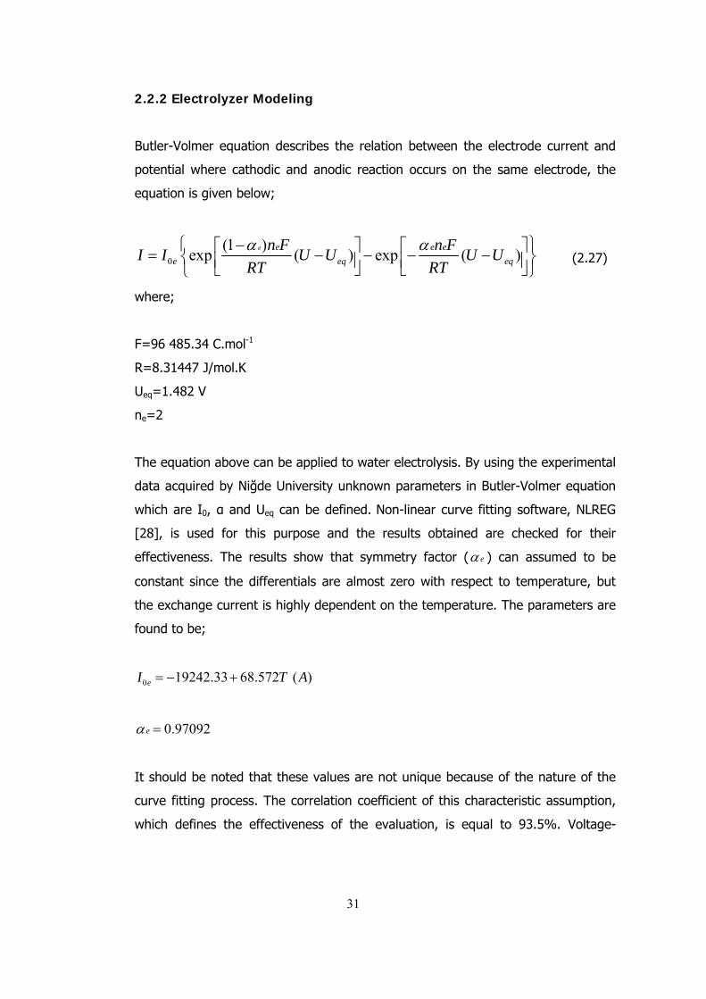
2.2.2 Electrolyzer Modeling

Butler-Volmer equation describes the relation between the electrode current and

potential where cathodic and anodic reaction occurs on the same electrode, the

equation is given below;

0

(1 )exp ( ) exp ( )

e e e e

e eq eq

n F n FI I U U U U

RT RT

(2.27)

where;

F=96 485.34 C.mol-1

R=8.31447 J/mol.K

Ueq=1.482 V

ne=2

The equation above can be applied to water electrolysis. By using the experimental

data acquired by Niğde University unknown parameters in Butler-Volmer equation

which are I0, α and Ueq can be defined. Non-linear curve fitting software, NLREG

[28], is used for this purpose and the results obtained are checked for their

effectiveness. The results show that symmetry factor ( e ) can assumed to be

constant since the differentials are almost zero with respect to temperature, but

the exchange current is highly dependent on the temperature. The parameters are

found to be;

0 19242.33 68.572 ( )eI T A

0.97092e

It should be noted that these values are not unique because of the nature of the

curve fitting process. The correlation coefficient of this characteristic assumption,

which defines the effectiveness of the evaluation, is equal to 93.5%. Voltage-

31

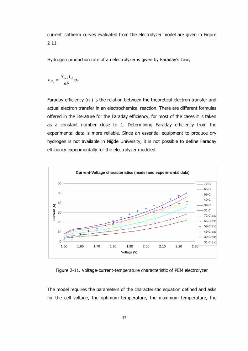
current isotherm curves evaluated from the electrolyzer model are given in Figure

2-11.

Hydrogen production rate of an electrolyzer is given by Faraday’s Law;

2

cell elFH

N In

nF

Faraday efficiency (ηF) is the relation between the theoretical electron transfer and

actual electron transfer in an electrochemical reaction. There are different formulas

offered in the literature for the Faraday efficiency, for most of the cases it is taken

as a constant number close to 1. Determining Faraday efficiency from the

experimental data is more reliable. Since an essential equipment to produce dry

hydrogen is not available in Niğde University, it is not possible to define Faraday

efficiency experimentally for the electrolyzer modeled.

Current-Voltage characteristics (model and experimental data)

0

10

20

30

40

50

60

1.50 1.60 1.70 1.80 1.90 2.00 2.10 2.20 2.30

Voltage (V)

Cu

rre

nt

(A)

72 C

65 C

59 C

49 C

39 C

31 C

72 C exp

65 C exp

59 C exp

49 C exp

39 C exp

31 C exp

Figure 2-11. Voltage-current-temperature characteristic of PEM electrolyzer

The model requires the parameters of the characteristic equation defined and asks

for the cell voltage, the optimum temperature, the maximum temperature, the

32

number of series connected cells in a stack, total number of parallel connected

stacks and power supplied to the electrolyzer. The model first evaluates the

maximum power that the electrolyzer operate at from the given inputs number of

cells, number of stacks and maximum temperature. If the power supplied is

greater than maximum power, the extra power is dumped away. The model tries

to operate as close as possible to optimum temperature provided by the user. With

respect to supplied electrical power, the number of electrolyzer stacks in operation

is optimized to have the cell temperature as close as possible to optimum

temperature. By this way, electrolyzer produces a respectable amount of hydrogen

with decent efficiency and temperature. 50oC optimum temperature and 2V cell

voltage is selected for the simulations as the manufacturers offer. FORTRAN code

of the model is given in Appendix C.

33

5 CHAPTER 3

SYSTEM SIMULATIONS

System simulations are conducted with TRNSYS. PV panel and PEM electrolyzer

models have been implemented in the software. Together with the user-defined

and default components, a solar stand alone power system is simulated. Different

system scenarios and component sizes are tested for yearly simulations.

3.1 System Description

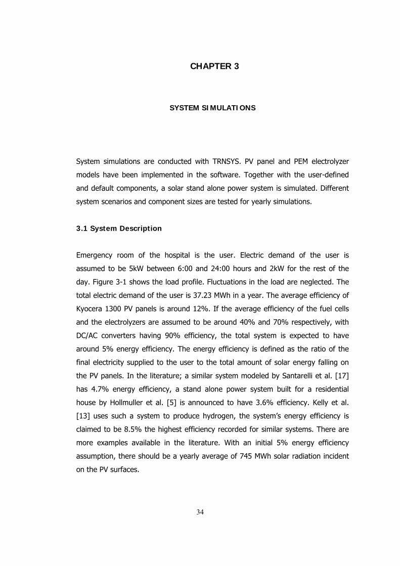
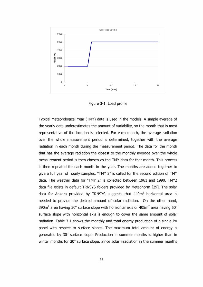
Emergency room of the hospital is the user. Electric demand of the user is

assumed to be 5kW between 6:00 and 24:00 hours and 2kW for the rest of the

day. Figure 3-1 shows the load profile. Fluctuations in the load are neglected. The

total electric demand of the user is 37.23 MWh in a year. The average efficiency of

Kyocera 1300 PV panels is around 12%. If the average efficiency of the fuel cells

and the electrolyzers are assumed to be around 40% and 70% respectively, with

DC/AC converters having 90% efficiency, the total system is expected to have

around 5% energy efficiency. The energy efficiency is defined as the ratio of the

final electricity supplied to the user to the total amount of solar energy falling on

the PV panels. In the literature; a similar system modeled by Santarelli et al. [17]

has 4.7% energy efficiency, a stand alone power system built for a residential

house by Hollmuller et al. [5] is announced to have 3.6% efficiency. Kelly et al.

[13] uses such a system to produce hydrogen, the system’s energy efficiency is

claimed to be 8.5% the highest efficiency recorded for similar systems. There are

more examples available in the literature. With an initial 5% energy efficiency

assumption, there should be a yearly average of 745 MWh solar radiation incident

on the PV surfaces.

34

User load vs time

0

1000

2000

3000

4000

5000

6000

0 6 12 18 24

Time (hour)

Po

we

r (W

)

Figure 3-1. Load profile

Typical Meteorological Year (TMY) data is used in the models. A simple average of

the yearly data underestimates the amount of variability, so the month that is most

representative of the location is selected. For each month, the average radiation

over the whole measurement period is determined, together with the average

radiation in each month during the measurement period. The data for the month

that has the average radiation the closest to the monthly average over the whole

measurement period is then chosen as the TMY data for that month. This process

is then repeated for each month in the year. The months are added together to

give a full year of hourly samples. “TMY 2” is called for the second edition of TMY

data. The weather data for “TMY 2” is collected between 1961 and 1990. TMY2

data file exists in default TRNSYS folders provided by Meteonorm [29]. The solar

data for Ankara provided by TRNSYS suggests that 440m2 horizontal area is

needed to provide the desired amount of solar radiation. On the other hand,

390m2 area having 30o surface slope with horizontal axis or 405m2 area having 50o

surface slope with horizontal axis is enough to cover the same amount of solar

radiation. Table 3-1 shows the monthly and total energy production of a single PV

panel with respect to surface slopes. The maximum total amount of energy is

generated by 30o surface slope. Production in summer months is higher than in

winter months for 30o surface slope. Since solar irradiation in the summer months

35

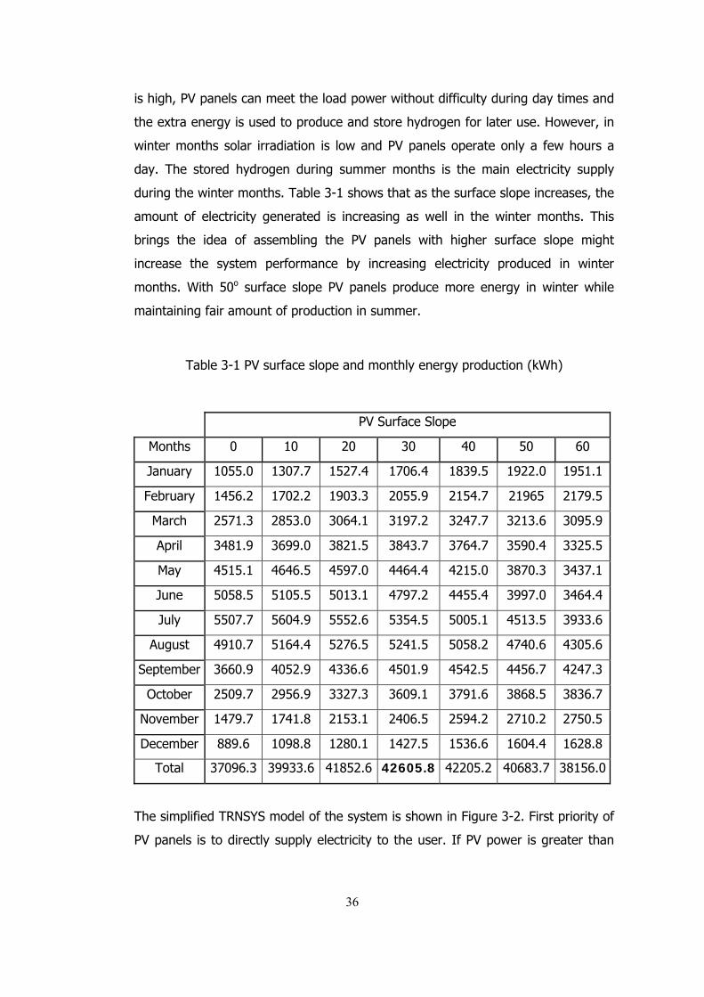
is high, PV panels can meet the load power without difficulty during day times and

the extra energy is used to produce and store hydrogen for later use. However, in

winter months solar irradiation is low and PV panels operate only a few hours a

day. The stored hydrogen during summer months is the main electricity supply

during the winter months. Table 3-1 shows that as the surface slope increases, the

amount of electricity generated is increasing as well in the winter months. This

brings the idea of assembling the PV panels with higher surface slope might

increase the system performance by increasing electricity produced in winter

months. With 50o surface slope PV panels produce more energy in winter while

maintaining fair amount of production in summer.

Table 3-1 PV surface slope and monthly energy production (kWh)

PV Surface Slope

Months 0 10 20 30 40 50 60

January 1055.0 1307.7 1527.4 1706.4 1839.5 1922.0 1951.1

February 1456.2 1702.2 1903.3 2055.9 2154.7 21965 2179.5

March 2571.3 2853.0 3064.1 3197.2 3247.7 3213.6 3095.9

April 3481.9 3699.0 3821.5 3843.7 3764.7 3590.4 3325.5

May 4515.1 4646.5 4597.0 4464.4 4215.0 3870.3 3437.1

June 5058.5 5105.5 5013.1 4797.2 4455.4 3997.0 3464.4

July 5507.7 5604.9 5552.6 5354.5 5005.1 4513.5 3933.6

August 4910.7 5164.4 5276.5 5241.5 5058.2 4740.6 4305.6

September 3660.9 4052.9 4336.6 4501.9 4542.5 4456.7 4247.3

October 2509.7 2956.9 3327.3 3609.1 3791.6 3868.5 3836.7

November 1479.7 1741.8 2153.1 2406.5 2594.2 2710.2 2750.5

December 889.6 1098.8 1280.1 1427.5 1536.6 1604.4 1628.8

Total 37096.3 39933.6 41852.6 42605.8 42205.2 40683.7 38156.0

The simplified TRNSYS model of the system is shown in Figure 3-2. First priority of

PV panels is to directly supply electricity to the user. If PV power is greater than

36

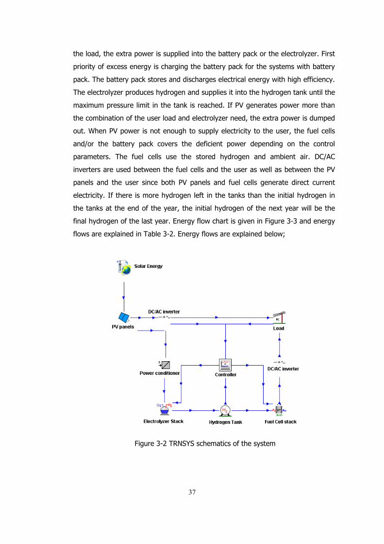
the load, the extra power is supplied into the battery pack or the electrolyzer. First

priority of excess energy is charging the battery pack for the systems with battery

pack. The battery pack stores and discharges electrical energy with high efficiency.

The electrolyzer produces hydrogen and supplies it into the hydrogen tank until the

maximum pressure limit in the tank is reached. If PV generates power more than

the combination of the user load and electrolyzer need, the extra power is dumped

out. When PV power is not enough to supply electricity to the user, the fuel cells

and/or the battery pack covers the deficient power depending on the control

parameters. The fuel cells use the stored hydrogen and ambient air. DC/AC

inverters are used between the fuel cells and the user as well as between the PV

panels and the user since both PV panels and fuel cells generate direct current

electricity. If there is more hydrogen left in the tanks than the initial hydrogen in

the tanks at the end of the year, the initial hydrogen of the next year will be the

final hydrogen of the last year. Energy flow chart is given in Figure 3-3 and energy

flows are explained in Table 3-2. Energy flows are explained below;

Figure 3-2 TRNSYS schematics of the system

37

Figu

re 3

-3 E

nerg

y Fl

ow c

hart

in t

he s

yste

m

PV

pan

els

Bu

sb

ar

Bat

tery

Sta

ck

Inve

rter

Au

xial

lary

eq

uip

men

t -C

ontr

ol p

anel

-H

2 pu

rifi

er

-H2O

dei

oniz

er

-H2

com

pres

sor

Ele

ctro

lyze

r

H2

(e

ner

gy c

arri

er)

Fu

el C

ell

Use

r

Du

mp

ed

Los

s

Los

s

Los

s L

oss

Los

s

E1

E2 E3

E4

E5

E6

E7

E8

E9

E10

E11

E12

Sol

ar E

ner

gy

38

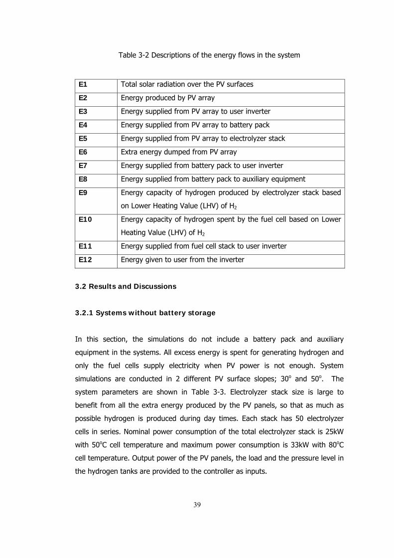
Table 3-2 Descriptions of the energy flows in the system

3.2 Results and Discussions

3.2.1 Systems without battery storage

In this section, the simulations do not include a battery pack and auxiliary

equipment in the systems. All excess energy is spent for generating hydrogen and

only the fuel cells supply electricity when PV power is not enough. System

simulations are conducted in 2 different PV surface slopes; 30o and 50o. The

system parameters are shown in Table 3-3. Electrolyzer stack size is large to

benefit from all the extra energy produced by the PV panels, so that as much as

possible hydrogen is produced during day times. Each stack has 50 electrolyzer

cells in series. Nominal power consumption of the total electrolyzer stack is 25kW

with 50oC cell temperature and maximum power consumption is 33kW with 80oC

cell temperature. Output power of the PV panels, the load and the pressure level in

the hydrogen tanks are provided to the controller as inputs.

E1 Total solar radiation over the PV surfaces

E2 Energy produced by PV array

E3 Energy supplied from PV array to user inverter

E4 Energy supplied from PV array to battery pack

E5 Energy supplied from PV array to electrolyzer stack

E6 Extra energy dumped from PV array

E7 Energy supplied from battery pack to user inverter

E8 Energy supplied from battery pack to auxiliary equipment

E9 Energy capacity of hydrogen produced by electrolyzer stack based

on Lower Heating Value (LHV) of H2

E10 Energy capacity of hydrogen spent by the fuel cell based on Lower

Heating Value (LHV) of H2

E11 Energy supplied from fuel cell stack to user inverter

E12 Energy given to user from the inverter

39

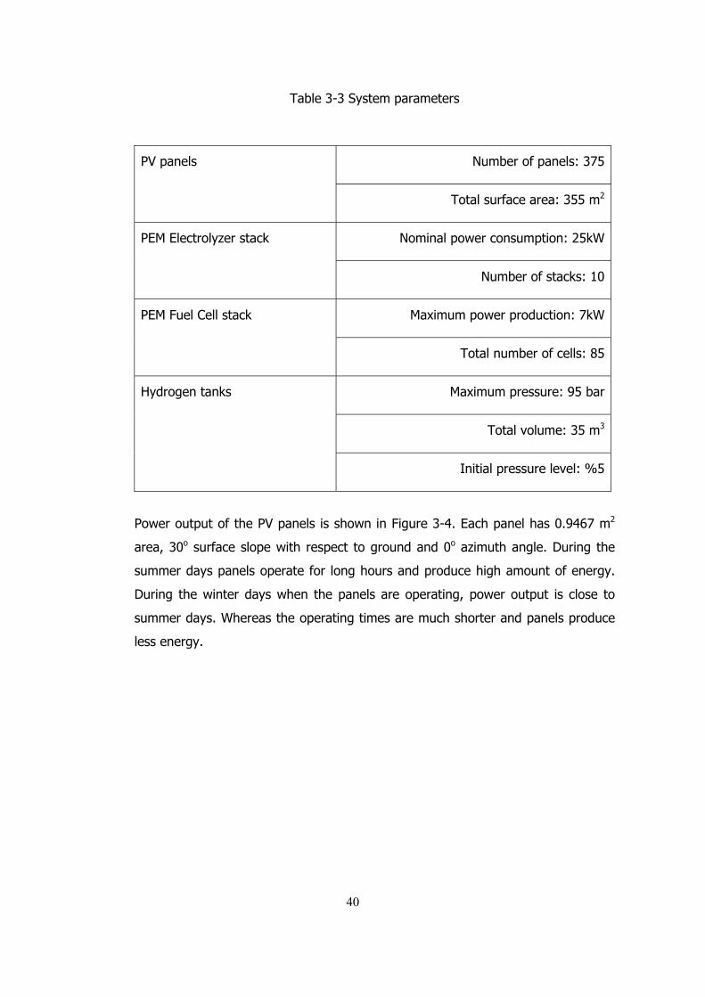
Table 3-3 System parameters

Number of panels: 375PV panels

Total surface area: 355 m2

Nominal power consumption: 25kWPEM Electrolyzer stack

Number of stacks: 10

Maximum power production: 7kW PEM Fuel Cell stack

Total number of cells: 85

Maximum pressure: 95 bar

Total volume: 35 m3

Hydrogen tanks

Initial pressure level: %5

Power output of the PV panels is shown in Figure 3-4. Each panel has 0.9467 m2

area, 30o surface slope with respect to ground and 0o azimuth angle. During the

summer days panels operate for long hours and produce high amount of energy.

During the winter days when the panels are operating, power output is close to

summer days. Whereas the operating times are much shorter and panels produce

less energy.

40

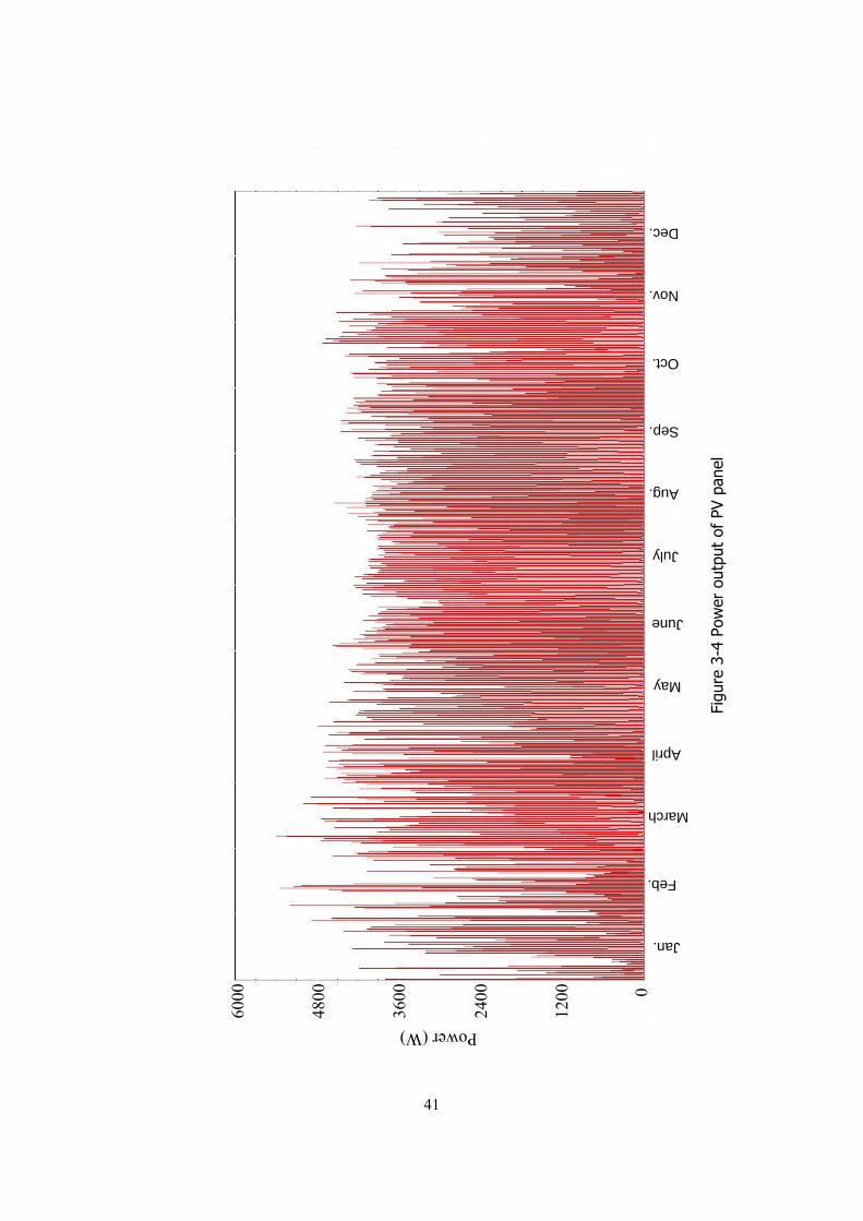
Figu

re 3

-4 P

ower

out

put

of P

V pa

nel

Dec.

Nov.

Feb.

Jan.

March

April

May

June

July

Aug.

Sep.

Oct.

6000

4800

3600

2400

1200

0

Power (W)

41

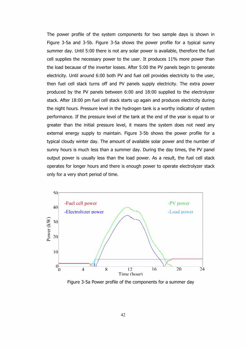
The power profile of the system components for two sample days is shown in

Figure 3-5a and 3-5b. Figure 3-5a shows the power profile for a typical sunny

summer day. Until 5:00 there is not any solar power is available, therefore the fuel

cell supplies the necessary power to the user. It produces 11% more power than

the load because of the inverter losses. After 5:00 the PV panels begin to generate

electricity. Until around 6:00 both PV and fuel cell provides electricity to the user,

then fuel cell stack turns off and PV panels supply electricity. The extra power

produced by the PV panels between 6:00 and 18:00 supplied to the electrolyzer

stack. After 18:00 pm fuel cell stack starts up again and produces electricity during

the night hours. Pressure level in the hydrogen tank is a worthy indicator of system

performance. If the pressure level of the tank at the end of the year is equal to or

greater than the initial pressure level, it means the system does not need any

external energy supply to maintain. Figure 3-5b shows the power profile for a

typical cloudy winter day. The amount of available solar power and the number of

sunny hours is much less than a summer day. During the day times, the PV panel

output power is usually less than the load power. As a result, the fuel cell stack

operates for longer hours and there is enough power to operate electrolyzer stack

only for a very short period of time.

Figure 3-5a Power profile of the components for a summer day

50

40

30

20

10

0

Pow

er (

kW)

-Fuel cell power

-Electrolyzer power

-PV power

-Load power

4 8 12 16 20 24Time (hour)

0

42

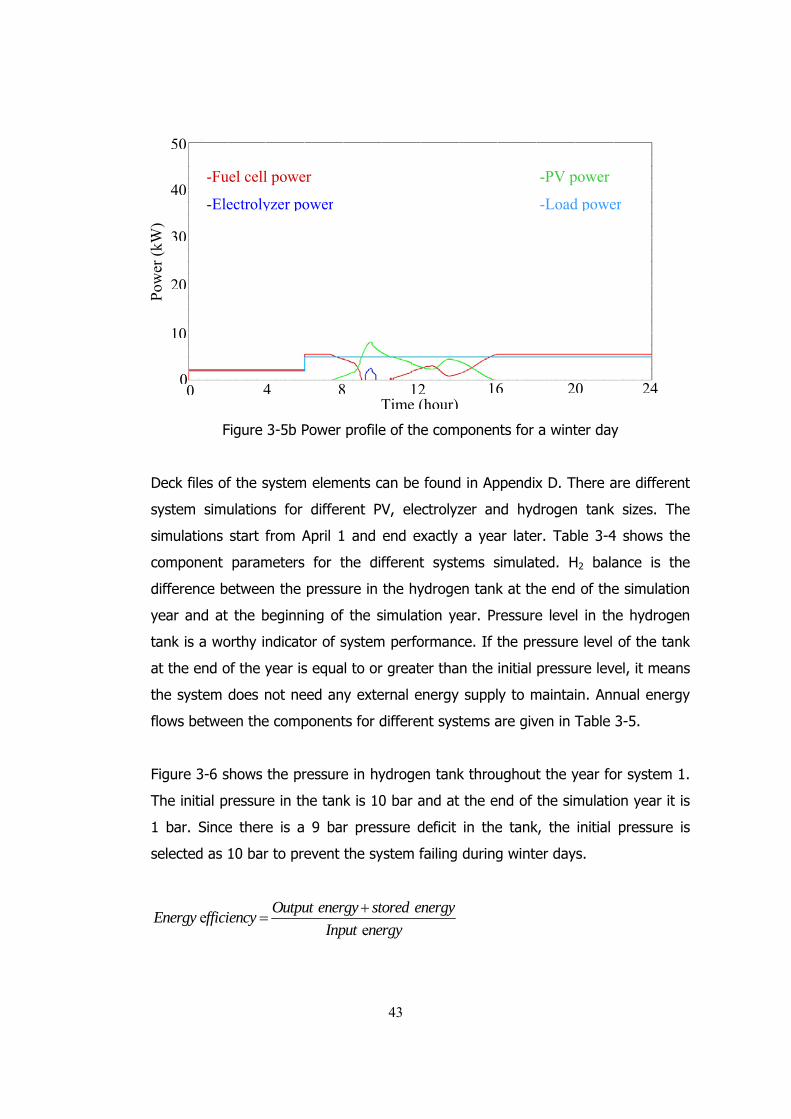
Figure 3-5b Power profile of the components for a winter day

Deck files of the system elements can be found in Appendix D. There are different

system simulations for different PV, electrolyzer and hydrogen tank sizes. The

simulations start from April 1 and end exactly a year later. Table 3-4 shows the

component parameters for the different systems simulated. H2 balance is the

difference between the pressure in the hydrogen tank at the end of the simulation

year and at the beginning of the simulation year. Pressure level in the hydrogen

tank is a worthy indicator of system performance. If the pressure level of the tank

at the end of the year is equal to or greater than the initial pressure level, it means

the system does not need any external energy supply to maintain. Annual energy

flows between the components for different systems are given in Table 3-5.

Figure 3-6 shows the pressure in hydrogen tank throughout the year for system 1.

The initial pressure in the tank is 10 bar and at the end of the simulation year it is

1 bar. Since there is a 9 bar pressure deficit in the tank, the initial pressure is

selected as 10 bar to prevent the system failing during winter days.

e

e

Output energy stored energyEnergy fficiency

Input nergy

50

40

30

20

10

0

Pow

er (

kW)

-Fuel cell power

-Electrolyzer power

-PV power

-Load power

4 8 12 16 20 24Time (hour)

0

43

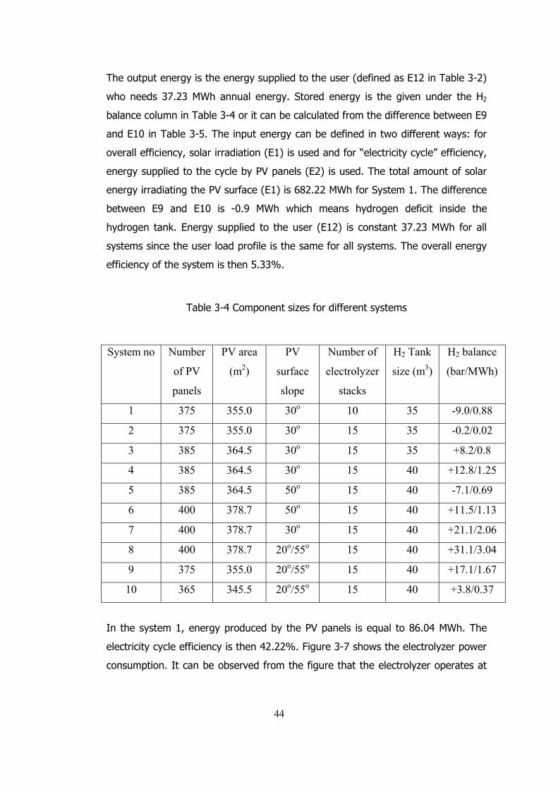
The output energy is the energy supplied to the user (defined as E12 in Table 3-2)

who needs 37.23 MWh annual energy. Stored energy is the given under the H2

balance column in Table 3-4 or it can be calculated from the difference between E9

and E10 in Table 3-5. The input energy can be defined in two different ways: for

overall efficiency, solar irradiation (E1) is used and for “electricity cycle” efficiency,

energy supplied to the cycle by PV panels (E2) is used. The total amount of solar

energy irradiating the PV surface (E1) is 682.22 MWh for System 1. The difference

between E9 and E10 is -0.9 MWh which means hydrogen deficit inside the

hydrogen tank. Energy supplied to the user (E12) is constant 37.23 MWh for all

systems since the user load profile is the same for all systems. The overall energy

efficiency of the system is then 5.33%.

Table 3-4 Component sizes for different systems

System no Number

of PV

panels

PV area

(m2)

PV

surface

slope

Number of

electrolyzer

stacks

H2 Tank

size (m3)

H2 balance

(bar/MWh)

1 375 355.0 30o 10 35 -9.0/0.88

2 375 355.0 30o 15 35 -0.2/0.02

3 385 364.5 30o 15 35 +8.2/0.8

4 385 364.5 30o 15 40 +12.8/1.25

5 385 364.5 50o 15 40 -7.1/0.69

6 400 378.7 50o 15 40 +11.5/1.13

7 400 378.7 30o 15 40 +21.1/2.06

8 400 378.7 20o/55o 15 40 +31.1/3.04

9 375 355.0 20o/55o 15 40 +17.1/1.67

10 365 345.5 20o/55o 15 40 +3.8/0.37

In the system 1, energy produced by the PV panels is equal to 86.04 MWh. The

electricity cycle efficiency is then 42.22%. Figure 3-7 shows the electrolyzer power

consumption. It can be observed from the figure that the electrolyzer operates at

44

the maximum allowable power of 33kW and at the maximum allowable

temperature of 80oC for long hours. As a result of this, the efficiency of electrolyzer

and the electrolyzer life-time drop because of the high cell temperature. Also 1.52

MWh energy is dumped from the electrolyzer stack to avoid further heating in the

cells. These losses can be reduced by increasing the number of stacks, but it will

increase the initial cost of the system as well.

45

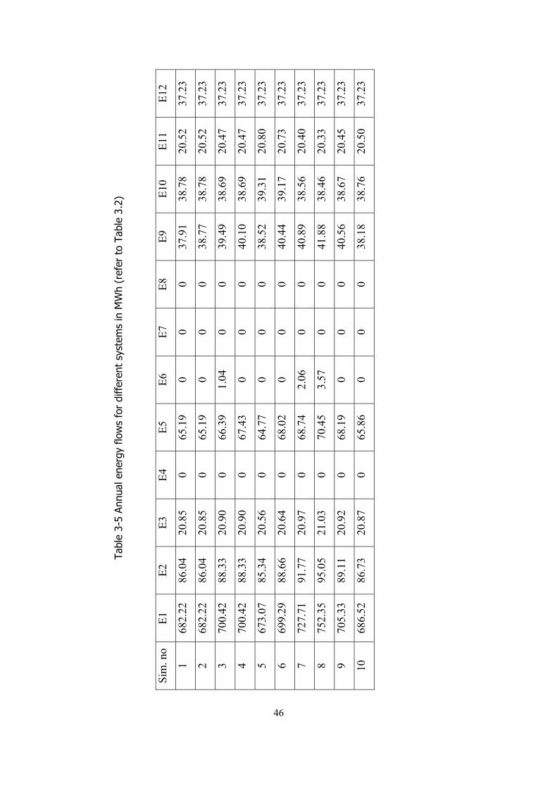
Tabl

e 3-

5 An

nual

ene

rgy

flow

s fo

r di

ffer

ent

syst

ems

in M

Wh

(ref

er t

o Ta

ble

3.2)

Sim

. no

E1

E2

E3

E4

E5

E6

E7

E8

E9

E10

E

11

E12

1 68

2.22

86

.04

20.8

5 0

65.1

9 0

0 0

37.9

1 38

.78

20.5

2 37

.23

2 68

2.22

86

.04

20.8

5 0

65.1

9 0

0 0

38.7

7 38

.78

20.5

2 37

.23

3 70

0.42

88

.33

20.9

0 0

66.3

9 1.

04

0 0

39.4

9 38

.69

20.4

7 37

.23

4 70

0.42

88

.33

20.9

0 0

67.4

3 0

0 0

40.1

0 38

.69

20.4

7 37

.23

5 67

3.07

85

.34

20.5

6 0

64.7

7 0

0 0

38.5

2 39

.31

20.8

0 37

.23

6 69

9.29

88

.66

20.6

4 0

68.0

2 0

0 0

40.4

4 39

.17

20.7

3 37

.23

7 72

7.71

91

.77

20.9

7 0

68.7

4 2.

06

0 0

40.8

9 38

.56

20.4

0 37

.23

8 75

2.35

95

.05

21.0

3 0

70.4

5 3.

57

0 0

41.8

8 38

.46

20.3

3 37

.23

9 70

5.33

89

.11

20.9

2 0

68.1

9 0

0 0

40.5

6 38

.67

20.4

5 37

.23

10

686.

52

86.7

3 20

.87

0 65

.86

0 0

0 38

.18

38.7

6 20

.50

37.2

3

46

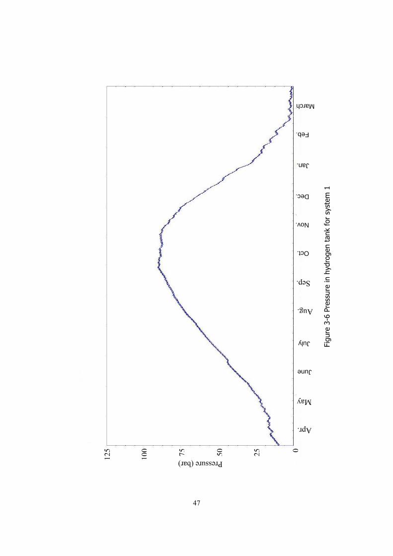
Figu

re 3

-6 P

ress

ure

in h

ydro

gen

tank

for

sys

tem

1

March

Feb.

May

Apr.

June

July

Aug.

Sep.

Oct.

Nov.

Dec.

Jan.

125

100 75 50 25 0

Pressure (bar)

47

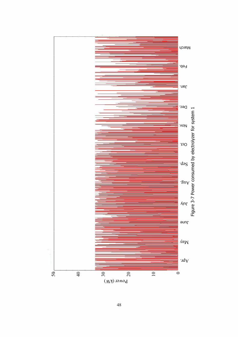
Figu

re 3

-7 P

ower

con

sum

ed b

y el

ectr

olyz

er f

or s

yste

m 1

March

Feb.

May

Apr.

June

July

Aug.

Sep.

Oct.

Nov.

Dec.

Jan.

50

40

30

20

10

0

Power (kW)

48

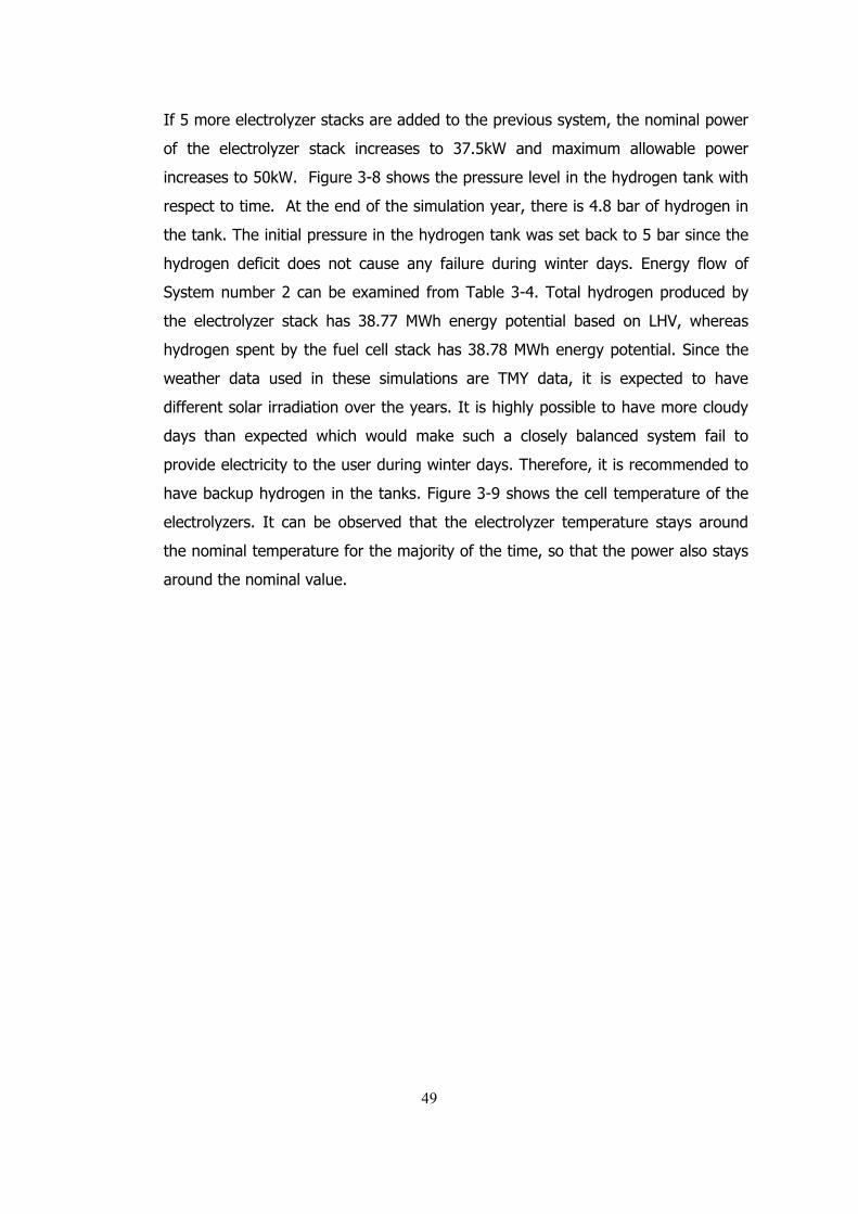
If 5 more electrolyzer stacks are added to the previous system, the nominal power

of the electrolyzer stack increases to 37.5kW and maximum allowable power

increases to 50kW. Figure 3-8 shows the pressure level in the hydrogen tank with

respect to time. At the end of the simulation year, there is 4.8 bar of hydrogen in

the tank. The initial pressure in the hydrogen tank was set back to 5 bar since the

hydrogen deficit does not cause any failure during winter days. Energy flow of

System number 2 can be examined from Table 3-4. Total hydrogen produced by

the electrolyzer stack has 38.77 MWh energy potential based on LHV, whereas

hydrogen spent by the fuel cell stack has 38.78 MWh energy potential. Since the

weather data used in these simulations are TMY data, it is expected to have

different solar irradiation over the years. It is highly possible to have more cloudy

days than expected which would make such a closely balanced system fail to

provide electricity to the user during winter days. Therefore, it is recommended to

have backup hydrogen in the tanks. Figure 3-9 shows the cell temperature of the

electrolyzers. It can be observed that the electrolyzer temperature stays around

the nominal temperature for the majority of the time, so that the power also stays

around the nominal value.

49

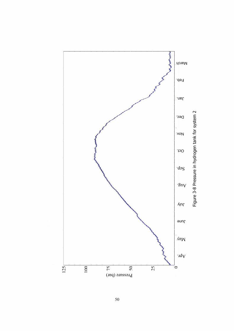
Figu

re 3

-8 P

ress

ure

in h

ydro

gen

tank

for

sys

tem

2

March

Feb.

May

Apr.

June

July

Aug.

Sep.

Oct.

Nov.

Dec.

Jan.

125

100 75 50 25 0

Pressure (bar)

50

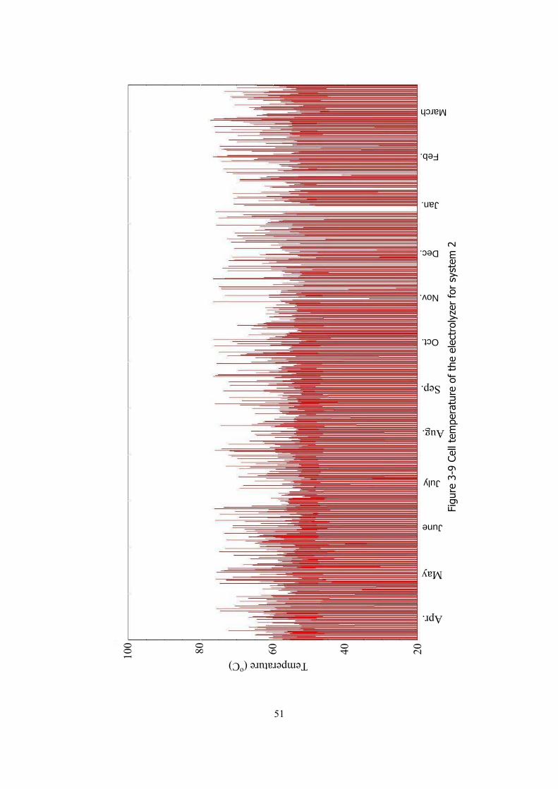
Fig

ure

3-9

Cell

tem

pera

ture

of

the

elec

trol

yzer

for

sys

tem

2

March

Feb.

May

Apr.

June

July

Aug.

Sep.

Oct.

Nov.

Dec.

Jan.

10

0

80

60

40

20

Temperature (oC)

51

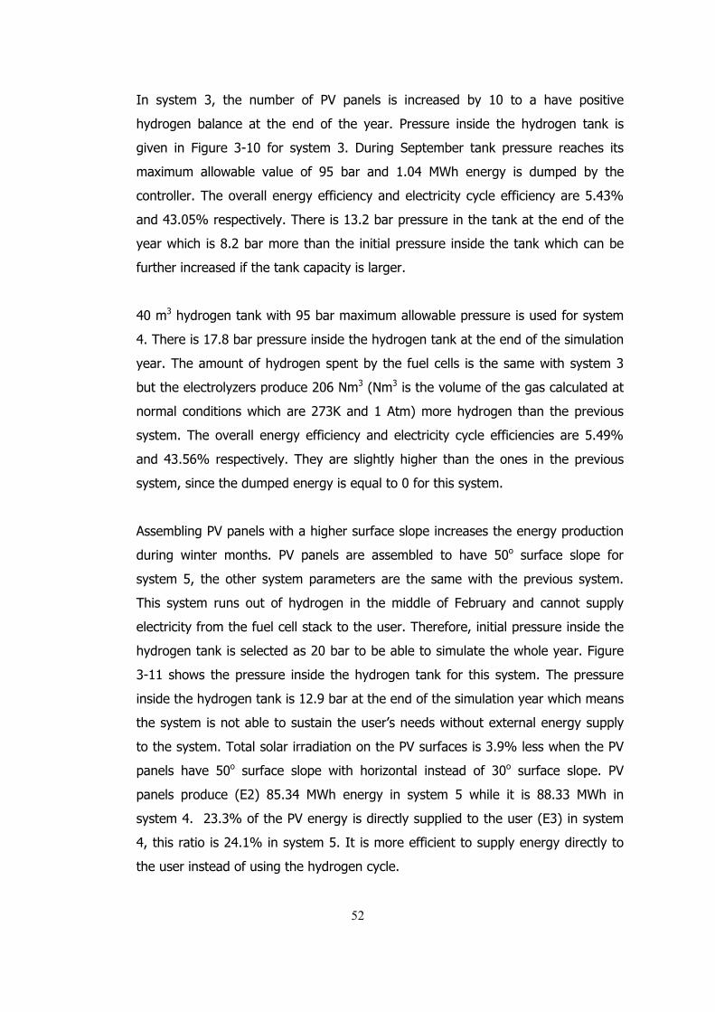
In system 3, the number of PV panels is increased by 10 to a have positive

hydrogen balance at the end of the year. Pressure inside the hydrogen tank is

given in Figure 3-10 for system 3. During September tank pressure reaches its

maximum allowable value of 95 bar and 1.04 MWh energy is dumped by the

controller. The overall energy efficiency and electricity cycle efficiency are 5.43%

and 43.05% respectively. There is 13.2 bar pressure in the tank at the end of the

year which is 8.2 bar more than the initial pressure inside the tank which can be

further increased if the tank capacity is larger.

40 m3 hydrogen tank with 95 bar maximum allowable pressure is used for system

4. There is 17.8 bar pressure inside the hydrogen tank at the end of the simulation

year. The amount of hydrogen spent by the fuel cells is the same with system 3

but the electrolyzers produce 206 Nm3 (Nm3 is the volume of the gas calculated at

normal conditions which are 273K and 1 Atm) more hydrogen than the previous

system. The overall energy efficiency and electricity cycle efficiencies are 5.49%

and 43.56% respectively. They are slightly higher than the ones in the previous

system, since the dumped energy is equal to 0 for this system.

Assembling PV panels with a higher surface slope increases the energy production

during winter months. PV panels are assembled to have 50o surface slope for

system 5, the other system parameters are the same with the previous system.

This system runs out of hydrogen in the middle of February and cannot supply

electricity from the fuel cell stack to the user. Therefore, initial pressure inside the

hydrogen tank is selected as 20 bar to be able to simulate the whole year. Figure

3-11 shows the pressure inside the hydrogen tank for this system. The pressure

inside the hydrogen tank is 12.9 bar at the end of the simulation year which means

the system is not able to sustain the user’s needs without external energy supply

to the system. Total solar irradiation on the PV surfaces is 3.9% less when the PV

panels have 50o surface slope with horizontal instead of 30o surface slope. PV

panels produce (E2) 85.34 MWh energy in system 5 while it is 88.33 MWh in

system 4. 23.3% of the PV energy is directly supplied to the user (E3) in system

4, this ratio is 24.1% in system 5. It is more efficient to supply energy directly to

the user instead of using the hydrogen cycle.

52

Figu

re 3

-10

Pres

sure

in h

ydro

gen

tank

for

sys

tem

3

March

Feb.

May

Apr.

June

July

Aug.

Sep.

Oct.

Nov.

Dec.

Jan.

125

100 75 50 25 0

Pressure (bar)

53

On the other hand, more hydrogen is spent in system 5 by the fuel cell stack

because the total amount of E3 is less than it was in the system 4. In system 4,

12897 Nm3 hydrogen is spent by the fuel cells while 13368 Nm3 hydrogen is

produced by the electrolyzers. Whereas; in system 5, 13103 Nm3 hydrogen is

spent by the fuel cells while 12841 Nm3 hydrogen is produced by the electrolyzer

stack. With 50o PV surface slope, the system produces less hydrogen and spends

more hydrogen. The overall and electricity efficiencies are 5.43% and 42.81%

respectively, they are less as well for this system.

In order to have positive hydrogen balance with 50o PV surface slope, the PV area

is increased for system 6. 400 PV panels are used in this system. The pressure

inside the hydrogen tank is 11.5 bar more than the initial value. Energy produced

by 400 PV panels with 50o surface slope is almost the same with the energy

produced by 385 PV panels with 30o surface slope. The overall and electricity

efficiencies are 5.49% and 43.27%. In system 7, PV surface slope is changed back

to 30o while keeping everything else the same as system 6. There is 26.1 bar

pressure inside the hydrogen tank at the end of the year. The overall and electric

efficiencies are 5.4% and 42.81% which are lower than the previous system. The

reason for this is 2.06 MWh energy dumped (E6) by the controller. The maximum

allowable tank pressure is reached during September as it can be observed from

Figure 3-12.

54

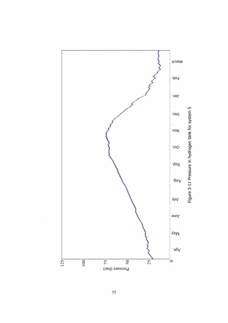
Figu

re 3

-11

Pres

sure

in h

ydro

gen

tank

for

sys

tem

5

March

Feb.

May

Apr.

June

July

Aug.

Sep.

Oct.

Nov.

Dec.

Jan.

125

100 75 50 25 0

Pressure (bar)

55

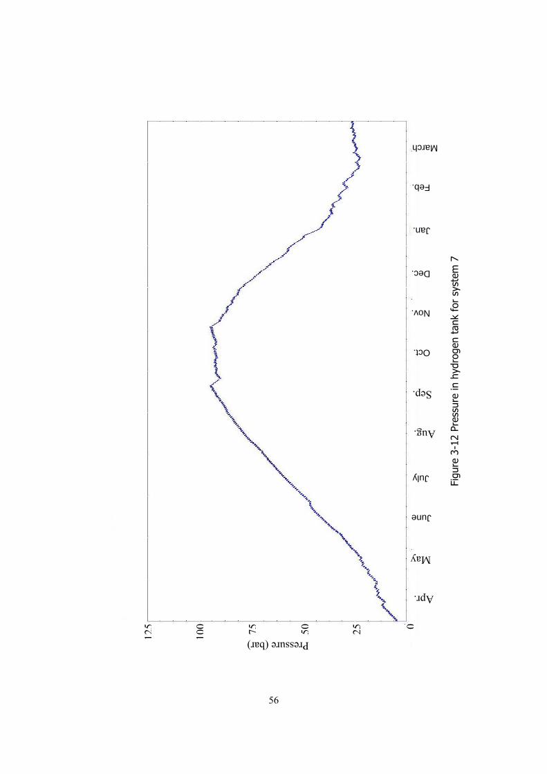
Figu

re 3

-12

Pres

sure

in h

ydro

gen

tank

for

sys

tem

7

March

Feb.

May

Apr.

June

July

Aug.

Sep.

Oct.

Nov.

Dec.

Jan.

125

100 75 50 25 0

Pressure (bar)

56

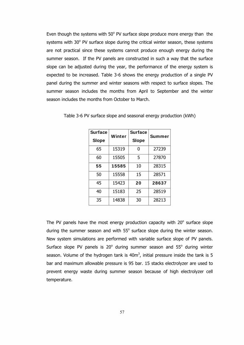
Even though the systems with 50o PV surface slope produce more energy than the

systems with 30o PV surface slope during the critical winter season, these systems

are not practical since these systems cannot produce enough energy during the

summer season. If the PV panels are constructed in such a way that the surface

slope can be adjusted during the year, the performance of the energy system is

expected to be increased. Table 3-6 shows the energy production of a single PV

panel during the summer and winter seasons with respect to surface slopes. The

summer season includes the months from April to September and the winter

season includes the months from October to March.

Table 3-6 PV surface slope and seasonal energy production (kWh)

Surface

Slope Winter

Surface

Slope Summer

65 15319 0 27239

60 15505 5 27870

55 15585 10 28315

50 15558 15 28571

45 15423 20 28637

40 15183 25 28519

35 14838 30 28213

The PV panels have the most energy production capacity with 20o surface slope

during the summer season and with 55o surface slope during the winter season.

New system simulations are performed with variable surface slope of PV panels.

Surface slope PV panels is 20o during summer season and 55o during winter

season. Volume of the hydrogen tank is 40m3, initial pressure inside the tank is 5

bar and maximum allowable pressure is 95 bar. 15 stacks electrolyzer are used to

prevent energy waste during summer season because of high electrolyzer cell

temperature.

57

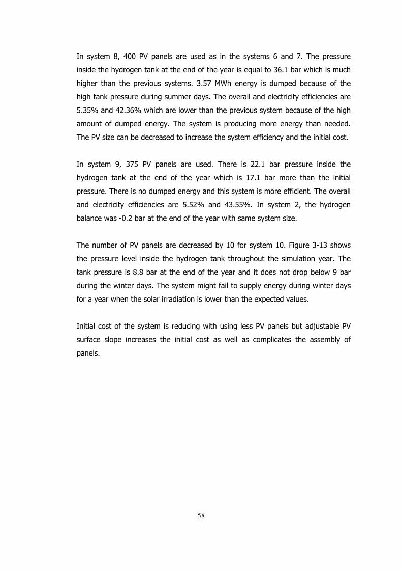
In system 8, 400 PV panels are used as in the systems 6 and 7. The pressure

inside the hydrogen tank at the end of the year is equal to 36.1 bar which is much

higher than the previous systems. 3.57 MWh energy is dumped because of the

high tank pressure during summer days. The overall and electricity efficiencies are

5.35% and 42.36% which are lower than the previous system because of the high

amount of dumped energy. The system is producing more energy than needed.

The PV size can be decreased to increase the system efficiency and the initial cost.

In system 9, 375 PV panels are used. There is 22.1 bar pressure inside the

hydrogen tank at the end of the year which is 17.1 bar more than the initial

pressure. There is no dumped energy and this system is more efficient. The overall

and electricity efficiencies are 5.52% and 43.55%. In system 2, the hydrogen

balance was -0.2 bar at the end of the year with same system size.

The number of PV panels are decreased by 10 for system 10. Figure 3-13 shows

the pressure level inside the hydrogen tank throughout the simulation year. The

tank pressure is 8.8 bar at the end of the year and it does not drop below 9 bar

during the winter days. The system might fail to supply energy during winter days

for a year when the solar irradiation is lower than the expected values.

Initial cost of the system is reducing with using less PV panels but adjustable PV

surface slope increases the initial cost as well as complicates the assembly of

panels.

58

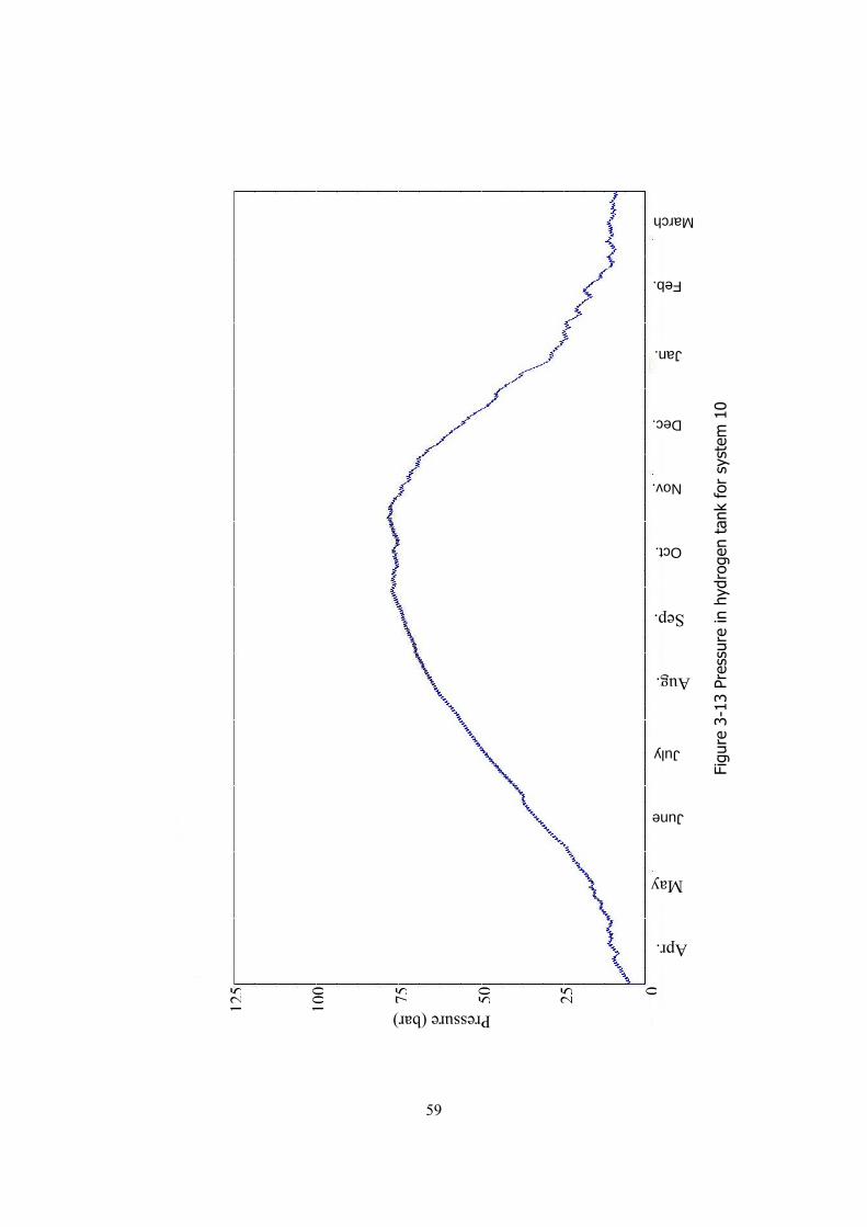
Figu

re 3

-13

Pres

sure

in h

ydro

gen

tank

for

sys

tem

10

March

Feb.

May

Apr.

June

July

Aug.

Sep.

Oct.

Nov.

Dec.

Jan.

125

100 75 50 25 0

Pressure (bar)

59

3.2.2 Systems with battery storage

The electrolyzer manufactured by Niğde Uni. works at 75% energy efficiency at the

operating conditions and PEM fuel cell used in the simulations has an average 40%

efficiency. Energy efficiency of the electrolyzer is defined as the ratio between

thermoneutral cell voltage and cell operating voltage. The electrolyzer cells are

designed to work at constant 2V. The total efficiency of the electrolyzer decreases

more when Faraday efficiency is taken into account as well which defines the

relation between actual and ideal flow rate of product hydrogen. If it is assumed

that there is no other loss in the hydrogen cycle and no auxiliary equipment energy

consumption, converting electric energy into chemical energy by means of

hydrogen and converting the chemical energy back to electric energy has less than

30% efficiency. When the energy consumption of water pumps, hydrogen and

water purifiers, controllers and inverters is added to the calculation, the overall

hydrogen cycle efficiency drops further more. On the other hand, batteries have

high efficiencies and do not require any auxiliary equipment, a usual Lead-acid

battery has more than 90% charging efficiency. It is more efficient and economic

to use batteries instead of hydrogen cycle for storing energy. However, energy

storage capacity of a battery is considerably low with respect to hydrogen storage

equipment. Because of this reason, it is not practical to use batteries for seasonal

storage, yet they can be used for daily storage.

Operating strategy of the battery stack is to help fuel cell during low insolation

hours. The aim is to increase the fuel cell efficiency by decreasing its load and

supplying a portion of the required electrical power by the battery stack that has a

high energy conversion efficiency. The simplified TRNSYS schematics of the system

is shown in Figure 3-14. A maximum desired operating power of the fuel cell is set

for the new system with battery stack. When the user needs more power than the

fuel cell maximum desired operating power, the battery stack will provide the

electricity. By this way, the energy spent on the inefficient hydrogen cycle will be

decreased and fuel cell efficiency will be increased since the fuel cells operate

more efficient at lower loads. The battery stack has a maximum and a minimum

allowable fractional state of charges (SOCmax and SOCmin) set to 0.8 and 0.4

60

because of the safety and efficiency reasons. Fractional state of charge is the ratio

between the total amount of energy stored in the battery and the total energy

capacity of the battery. For usual Lead-acid batteries, charging efficiency drops if

SOC is over 0.9 and life time of batteries becomes shorter if they operate at low

SOC levels. When battery SOC drops below the minimum allowable value, fuel cell

supplies all of the load power. Extra energy provided by the PV array is first

supplied to the battery stack if SOC is lower than SOCmax. When SOCmax is reached

or PV power is greater than the maximum allowable charging power (which is

selected as 20kW for this battery stack), extra power from the PV array is supplied

to the electrolyzer for hydrogen production.

The system parameters for the conducted simulations are given in Table 3-7.

Constant PV surface slope of 30o and electrolyzer size of 15 stacks are used

considering the results in the previous section. Hydrogen tank size is kept at 35 m3

since there is the battery pack also helping to the energy storage. Battery start up

power is equal to the maximum desired power of the fuel cells. When the power

deficit between the user load and the solar energy is less than the battery start up

power, only the fuel cells will work. When the power deficit is more than the

battery start up power, battery stack will also supply the power with the fuel cells.

The energy flow values are given in Table 3-8 for the different systems. E8 is equal

to 0 for all systems since no auxiliary equipment is used in systems in this section.

The effects of the auxiliary equipment will be examined in the next section.

61

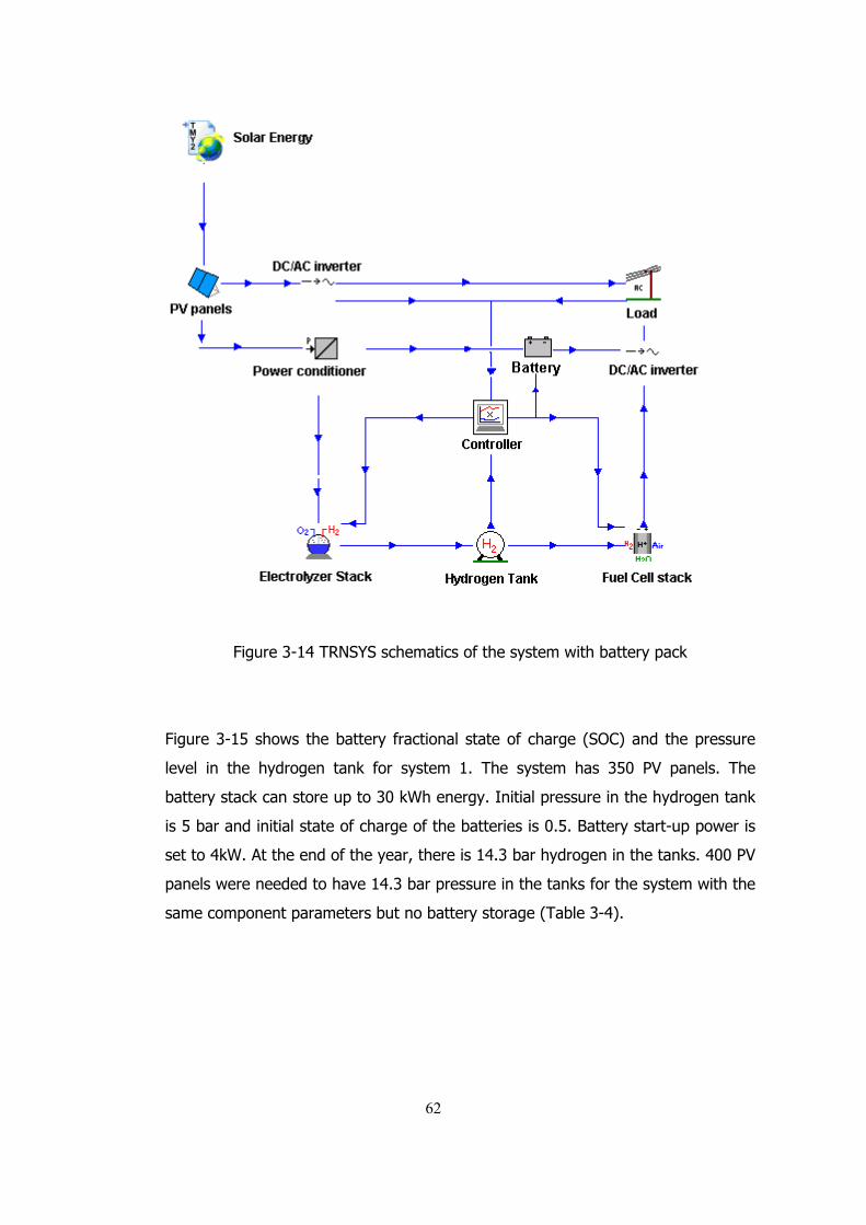
Figure 3-14 TRNSYS schematics of the system with battery pack

Figure 3-15 shows the battery fractional state of charge (SOC) and the pressure

level in the hydrogen tank for system 1. The system has 350 PV panels. The

battery stack can store up to 30 kWh energy. Initial pressure in the hydrogen tank

is 5 bar and initial state of charge of the batteries is 0.5. Battery start-up power is

set to 4kW. At the end of the year, there is 14.3 bar hydrogen in the tanks. 400 PV

panels were needed to have 14.3 bar pressure in the tanks for the system with the

same component parameters but no battery storage (Table 3-4).

62

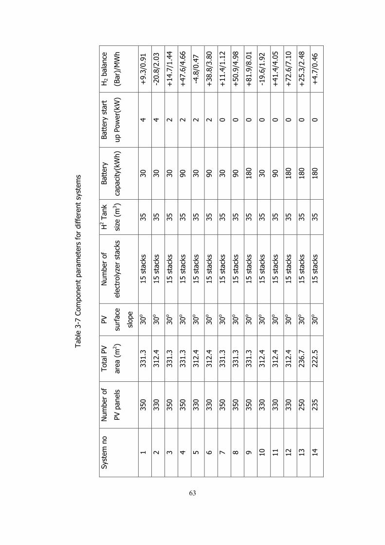
Tabl

e 3-

7 Co

mpo

nent

par

amet

ers

for

diff

eren

t sy

stem

s

Syst

em n

o N

umbe

r of

PV p

anel

s

Tota

l PV

area

(m

2 )

PV

surf

ace

slop

e

Num

ber

of

elec

trol

yzer

sta

cks

H2 T

ank

size

(m

3 )

Batt

ery

capa

city

(kW

h)

Batt

ery

star

t

up P

ower

(kW

)

H2

bala

nce

(Bar

)/M

Wh

1 35

0 33

1.3

30o

15 s

tack

s 35

30

4

+9.

3/0.

91

2 33

0 31

2.4

30o

15 s

tack

s 35

30

4

-20.

8/2.

03

3 35

0 33

1.3

30o

15 s

tack

s 35

30

2

+14

.7/1

.44

4 35

0 33

1.3

30o

15 s

tack

s 35

90

2

+47

.6/4

.66

5 33

0 31

2.4

30o

15 s

tack

s 35

30

2

-4.8

/0.4

7

6 33

0 31

2.4

30o

15 s

tack

s 35

90

2

+38

.8/3

.80

7 35

0 33

1.3

30o

15 s

tack

s 35

30

0

+11

.4/1

.12

8 35

0 33

1.3

30o

15 s

tack

s 35

90

0

+50

.9/4

.98

9 35

0 33

1.3

30o

15 s

tack

s 35

18

0 0

+81

.9/8

.01

10

330

312.

4 30

o 15

sta

cks

35

30

0 -1

9.6/

1.92

11

330

312.

4 30

o 15

sta

cks

35

90

0 +

41.4

/4.0

5

12

330

312.

4 30

o 15

sta

cks

35

180

0 +

72.6

/7.1

0

13

250

236.

7 30

o 15

sta

cks

35

180

0 +

25.3

/2.4

8

14

235

222.

5 30

o 15

sta

cks

35

180

0 +

4.7/

0.46

63

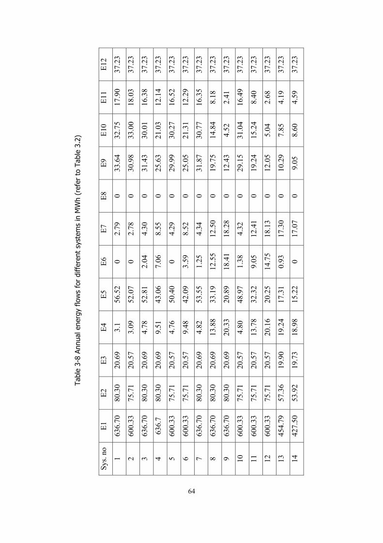
Tabl

e 3-

8 An

nual

ene

rgy

flow

s fo

r di

ffer

ent

syst

ems

in M

Wh

(ref

er t

o Ta

ble

3.2)

Sys

. no

E1

E2

E3

E4

E5

E6

E7

E8

E9

E10

E

11

E12

1 63

6.70

80

.30

20.6

9 3.

1 56

.52

0 2.

79

0 33

.64

32.7

5 17

.90

37.2

3

2 60

0.33

75

.71

20.5

7 3.

09

52.0

7 0

2.78

0

30.9

8 33

.00

18.0

3 37

.23

3 63

6.70

80

.30

20.6

9 4.

78

52.8

1 2.

04

4.30

0

31.4

3 30

.01

16.3

8 37

.23

4 63

6.7

80.3

0 20

.69

9.51

43

.06

7.06

8.

55

0 25

.63

21.0

3 12

.14

37.2

3

5 60

0.33

75

.71

20.5

7 4.

76

50.4

0 0

4.29

0

29.9

9 30

.27

16.5

2 37

.23

6 60

0.33

75

.71

20.5

7 9.

48

42.0

9 3.

59

8.52

0

25.0

5 21

.31

12.2

9 37

.23

7 63

6.70

80

.30

20.6

9 4.

82

53.5

5 1.

25

4.34

0

31.8

7 30

.77

16.3

5 37

.23

8 63

6.70

80

.30

20.6

9 13

.88

33.1

9 12

.55

12.5

0 0

19.7

5 14

.84

8.18

37

.23

9 63

6.70

80

.30

20.6

9 20

.33

20.8

9 18

.41

18.2

8 0

12.4

3 4.

52

2.41

37

.23

10

600.

33

75.7

1 20

.57

4.80

48

.97

1.38

4.

32

0 29

.15

31.0

4 16

.49

37.2

3

11

600.

33

75.7

1 20

.57

13.7

8 32

.32

9.05

12

.41

0 19

.24

15.2

4 8.

40

37.2

3

12

600.

33

75.7

1 20

.57

20.1

6 20

.25

14.7

5 18

.13

0 12

.05

5.04

2.

68

37.2

3

13

454.

79

57.3

6 19

.90

19.2

4 17

.31

0.93

17

.30

0 10

.29

7.85

4.

19

37.2

3

14

427.

50

53.9

2 19

.73

18.9

8 15

.22

0 17

.07

0 9.

05

8.60

4.

59

37.2

3

64

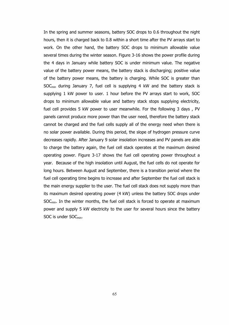
In the spring and summer seasons, battery SOC drops to 0.6 throughout the night

hours, then it is charged back to 0.8 within a short time after the PV arrays start to

work. On the other hand, the battery SOC drops to minimum allowable value

several times during the winter season. Figure 3-16 shows the power profile during

the 4 days in January while battery SOC is under minimum value. The negative

value of the battery power means, the battery stack is discharging; positive value

of the battery power means, the battery is charging. While SOC is greater than

SOCmin during January 7, fuel cell is supplying 4 kW and the battery stack is

supplying 1 kW power to user. 1 hour before the PV arrays start to work, SOC

drops to minimum allowable value and battery stack stops supplying electricity,

fuel cell provides 5 kW power to user meanwhile. For the following 3 days , PV

panels cannot produce more power than the user need, therefore the battery stack

cannot be charged and the fuel cells supply all of the energy need when there is

no solar power available. During this period, the slope of hydrogen pressure curve

decreases rapidly. After January 9 solar insolation increases and PV panels are able

to charge the battery again, the fuel cell stack operates at the maximum desired

operating power. Figure 3-17 shows the fuel cell operating power throughout a

year. Because of the high insolation until August, the fuel cells do not operate for

long hours. Between August and September, there is a transition period where the

fuel cell operating time begins to increase and after September the fuel cell stack is

the main energy supplier to the user. The fuel cell stack does not supply more than

its maximum desired operating power (4 kW) unless the battery SOC drops under

SOCmin. In the winter months, the fuel cell stack is forced to operate at maximum

power and supply 5 kW electricity to the user for several hours since the battery

SOC is under SOCmin.

65

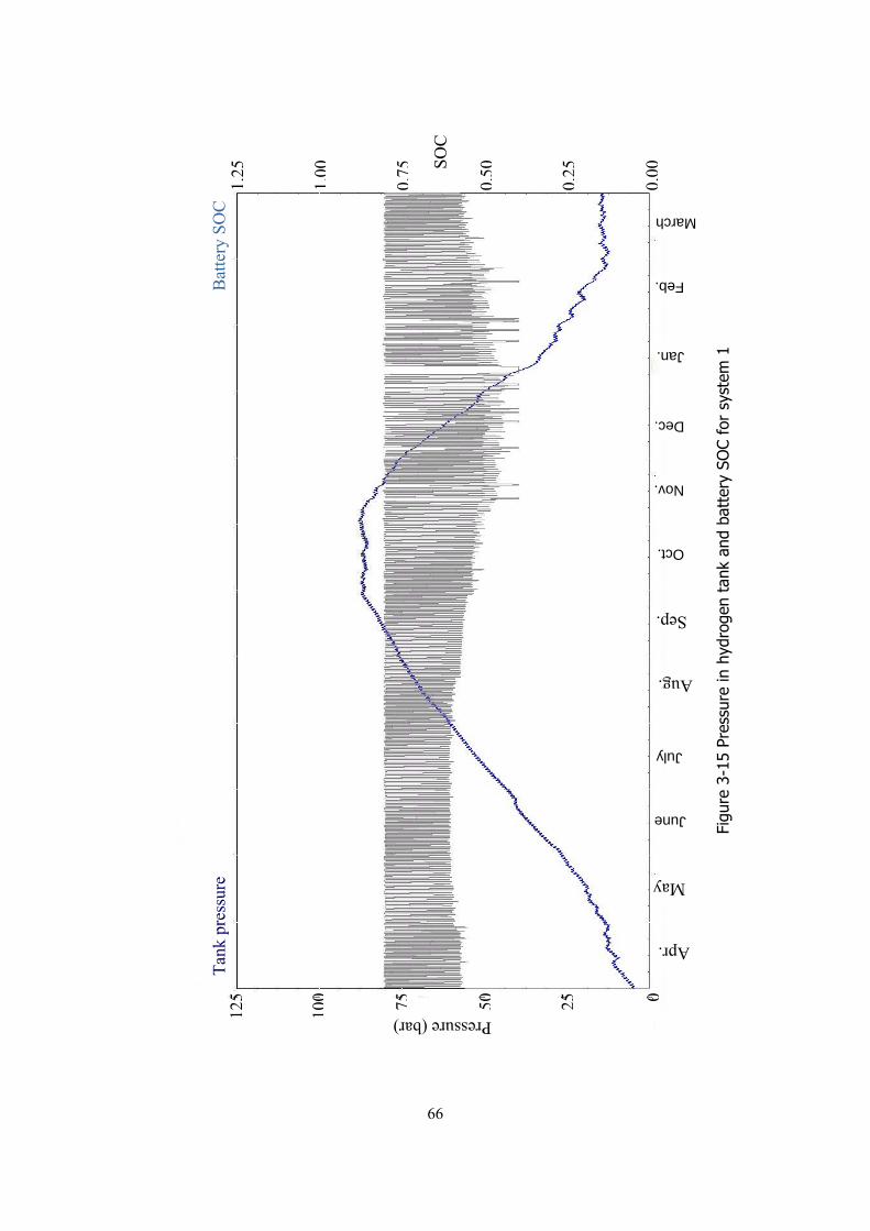
Figu

re 3

-15

Pres

sure

in h

ydro

gen

tank

and

bat

tery

SO

C fo

r sy

stem

1

March

Feb.

May

Apr.

June

July

Aug.

Sep.

Oct.

Nov.

Dec.

Jan.

Tan

k pr

essu

re

Bat

tery

SO

C

1.25

1.00

0.75

0.50

0.25

0.00SO

C

125

100 75 50 25 0

Pressure (bar)

66

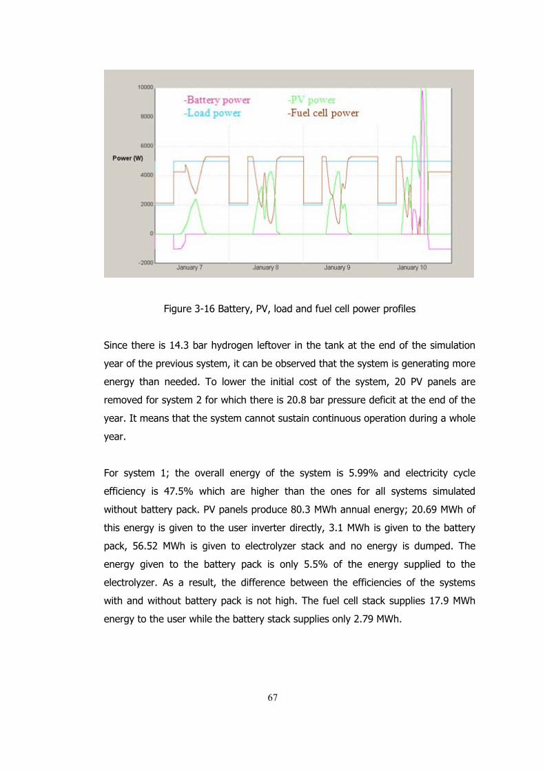
Figure 3-16 Battery, PV, load and fuel cell power profiles

Since there is 14.3 bar hydrogen leftover in the tank at the end of the simulation

year of the previous system, it can be observed that the system is generating more

energy than needed. To lower the initial cost of the system, 20 PV panels are

removed for system 2 for which there is 20.8 bar pressure deficit at the end of the

year. It means that the system cannot sustain continuous operation during a whole

year.

For system 1; the overall energy of the system is 5.99% and electricity cycle

efficiency is 47.5% which are higher than the ones for all systems simulated

without battery pack. PV panels produce 80.3 MWh annual energy; 20.69 MWh of

this energy is given to the user inverter directly, 3.1 MWh is given to the battery

pack, 56.52 MWh is given to electrolyzer stack and no energy is dumped. The

energy given to the battery pack is only 5.5% of the energy supplied to the

electrolyzer. As a result, the difference between the efficiencies of the systems

with and without battery pack is not high. The fuel cell stack supplies 17.9 MWh

energy to the user while the battery stack supplies only 2.79 MWh.

67

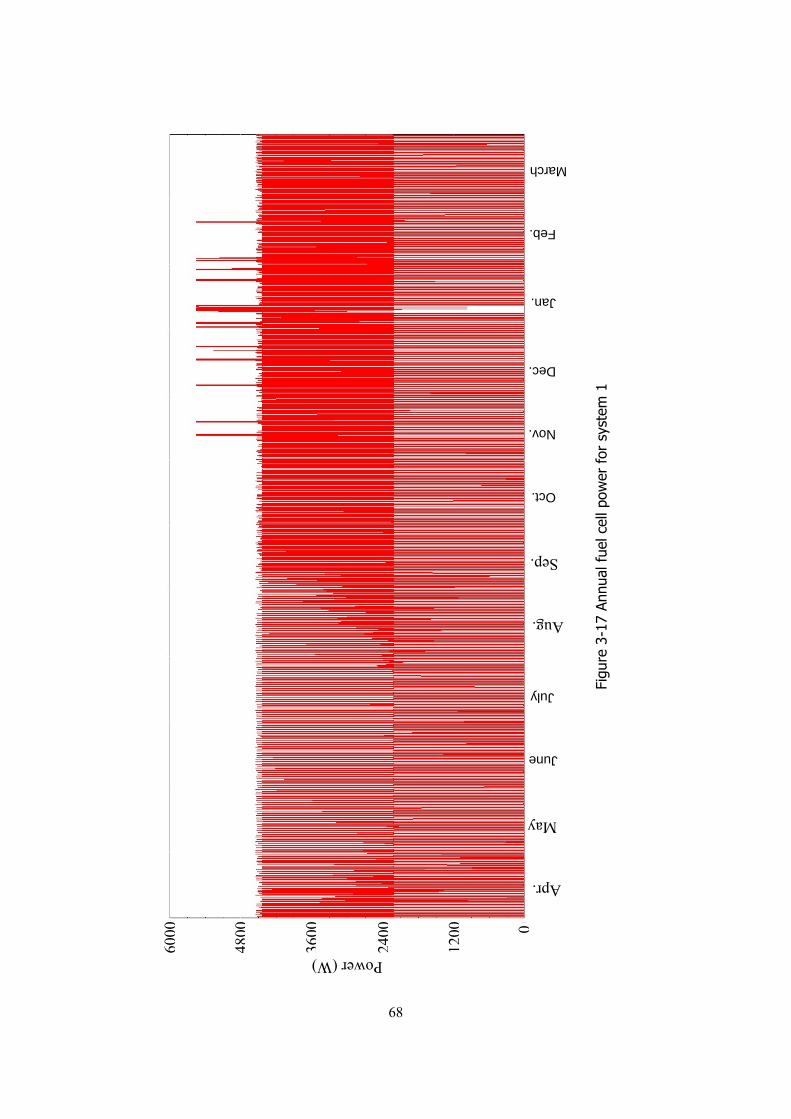
Figu

re 3

-17

Annu

al f

uel c

ell p

ower

for

sys

tem

1

March

Feb.

May

Apr.

June

July

Aug.

Sep.

Oct.

Nov.

Dec.

Jan.

6000

4800

3600

2400

1200 0

Power (W)

68

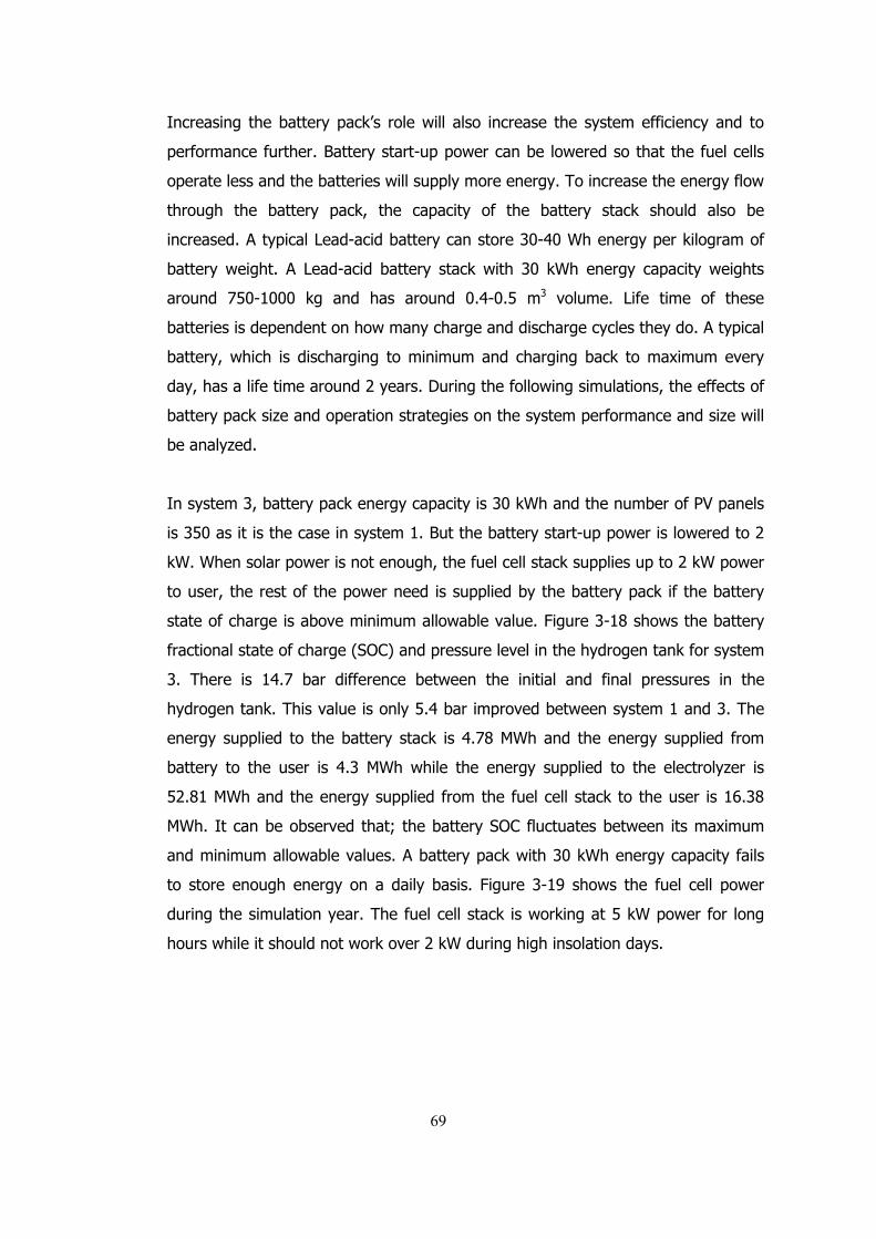
Increasing the battery pack’s role will also increase the system efficiency and to

performance further. Battery start-up power can be lowered so that the fuel cells

operate less and the batteries will supply more energy. To increase the energy flow

through the battery pack, the capacity of the battery stack should also be

increased. A typical Lead-acid battery can store 30-40 Wh energy per kilogram of

battery weight. A Lead-acid battery stack with 30 kWh energy capacity weights

around 750-1000 kg and has around 0.4-0.5 m3 volume. Life time of these

batteries is dependent on how many charge and discharge cycles they do. A typical

battery, which is discharging to minimum and charging back to maximum every

day, has a life time around 2 years. During the following simulations, the effects of

battery pack size and operation strategies on the system performance and size will

be analyzed.

In system 3, battery pack energy capacity is 30 kWh and the number of PV panels

is 350 as it is the case in system 1. But the battery start-up power is lowered to 2

kW. When solar power is not enough, the fuel cell stack supplies up to 2 kW power

to user, the rest of the power need is supplied by the battery pack if the battery

state of charge is above minimum allowable value. Figure 3-18 shows the battery

fractional state of charge (SOC) and pressure level in the hydrogen tank for system

3. There is 14.7 bar difference between the initial and final pressures in the

hydrogen tank. This value is only 5.4 bar improved between system 1 and 3. The

energy supplied to the battery stack is 4.78 MWh and the energy supplied from

battery to the user is 4.3 MWh while the energy supplied to the electrolyzer is

52.81 MWh and the energy supplied from the fuel cell stack to the user is 16.38

MWh. It can be observed that; the battery SOC fluctuates between its maximum

and minimum allowable values. A battery pack with 30 kWh energy capacity fails

to store enough energy on a daily basis. Figure 3-19 shows the fuel cell power

during the simulation year. The fuel cell stack is working at 5 kW power for long

hours while it should not work over 2 kW during high insolation days.

69

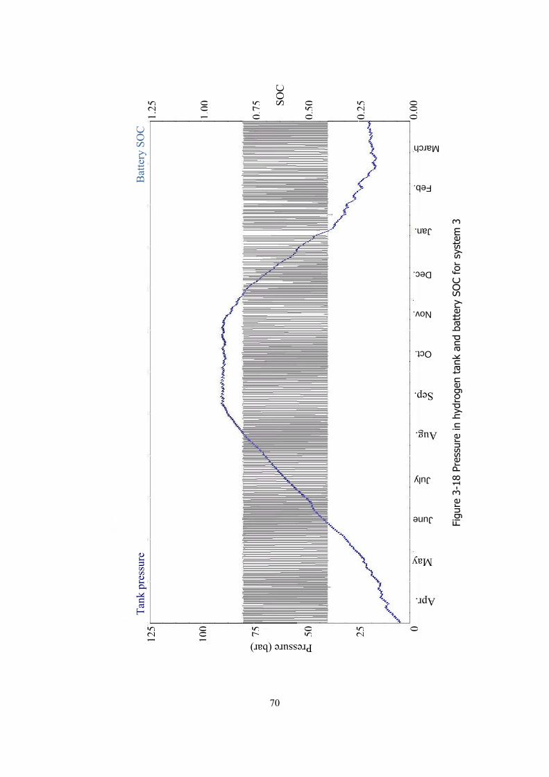
Figu

re 3

-18

Pres

sure

in h

ydro

gen

tank

and

bat

tery

SO

C fo

r sy

stem

3

March

Feb.

May

Apr.

June

July

Aug.

Sep.

Oct.

Nov.

Dec.

Jan.

Tan

k pr

essu

re

Bat

tery

SO

C

1.25

1.00

0.75

0.50

0.25

0.00SO

C

125

100 75 50 25 0

Pressure (bar)

70

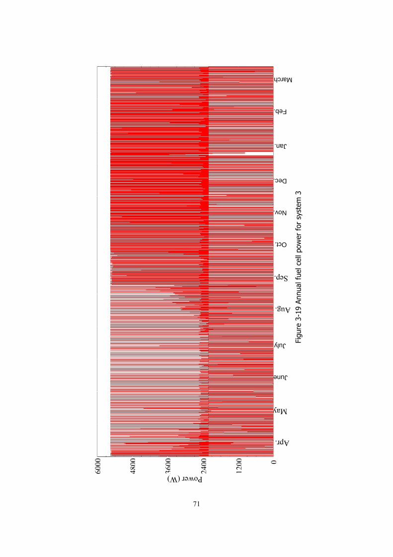
Figu

re 3

-19

Annu

al f

uel c

ell p

ower

for

sys

tem

3

March

Feb.

May

Apr.

June

July

Aug.

Sep.

Oct.

Nov.

Dec.

Jan.

6000

4800

3600

2400

1200 0

Power (W)

71

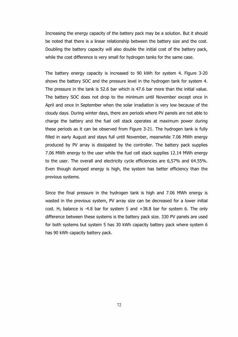
Increasing the energy capacity of the battery pack may be a solution. But it should

be noted that there is a linear relationship between the battery size and the cost.

Doubling the battery capacity will also double the initial cost of the battery pack,

while the cost difference is very small for hydrogen tanks for the same case.

The battery energy capacity is increased to 90 kWh for system 4. Figure 3-20

shows the battery SOC and the pressure level in the hydrogen tank for system 4.

The pressure in the tank is 52.6 bar which is 47.6 bar more than the initial value.

The battery SOC does not drop to the minimum until November except once in

April and once in September when the solar irradiation is very low because of the

cloudy days. During winter days, there are periods where PV panels are not able to

charge the battery and the fuel cell stack operates at maximum power during

these periods as it can be observed from Figure 3-21. The hydrogen tank is fully

filled in early August and stays full until November, meanwhile 7.06 MWh energy

produced by PV array is dissipated by the controller. The battery pack supplies

7.06 MWh energy to the user while the fuel cell stack supplies 12.14 MWh energy

to the user. The overall and electricity cycle efficiencies are 6,57% and 64.55%.

Even though dumped energy is high, the system has better efficiency than the

previous systems.

Since the final pressure in the hydrogen tank is high and 7.06 MWh energy is

wasted in the previous system, PV array size can be decreased for a lower initial

cost. H2 balance is -4.8 bar for system 5 and +38.8 bar for system 6. The only

difference between these systems is the battery pack size. 330 PV panels are used

for both systems but system 5 has 30 kWh capacity battery pack where system 6

has 90 kWh capacity battery pack.

72

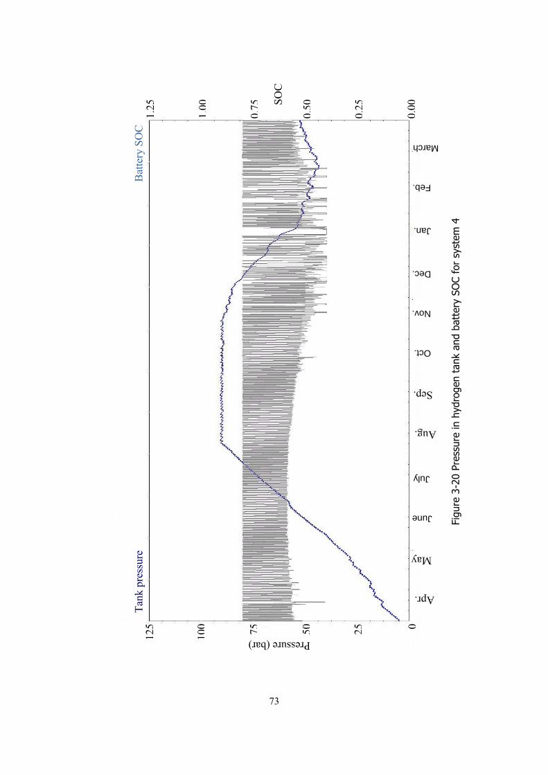
Figu

re 3

-20

Pres

sure

in h

ydro

gen

tank

and

bat

tery

SO

C fo

r sy

stem

4

March

Feb.

May

Apr.

June

July

Aug.

Sep.

Oct.

Nov.

Dec.

Jan.

Tan

k pr

essu

re

Bat

tery

SO

C

1.25

1.00

0.75

0.50

0.25

0.00SO

C

125

100 75 50 25 0

Pressure (bar)

73

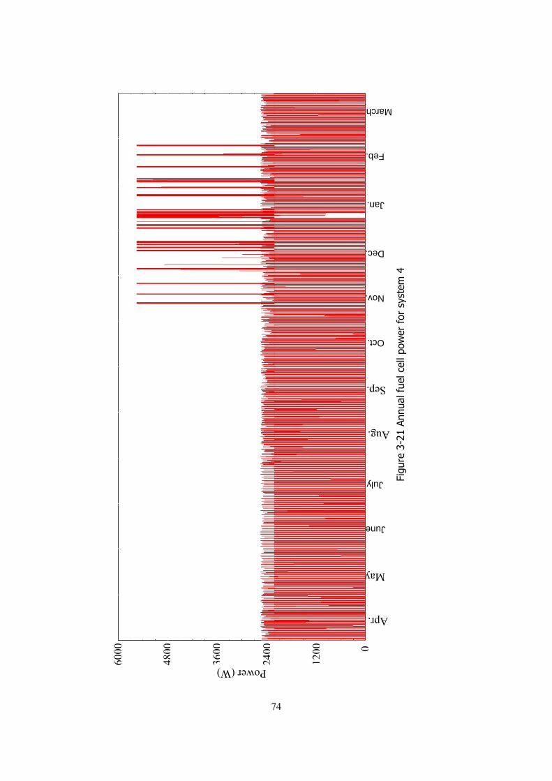
Figu

re 3

-21

Annu

al f

uel c

ell p

ower

for

sys

tem

4

March

Feb.

May

Apr.

June

July

Aug.

Sep.

Oct.

Nov.

Dec.

Jan.

6000

4800

3600

2400

1200 0

Power (W)

74

Another approach to managing solar energy is to use only the batteries for the

daily storage and to store hydrogen for the seasonal storage. The load profile of

the emergency room is shown in Figure 3-1, the daily energy need of the user is

102 kWh. The battery storage size should be more than this value because of the

maximum and minimum allowable state of charges and life time considerations of

the batteries. The battery pack always has priority to provide electricity to the

user. The fuel cell stack stays as a backup supplier and begins to operate during

the times when battery SOC drops under minimum allowable value. 8 different

simulations (system 7-14) are conducted for different PV and battery sizes. It can

be observed from Table 3-7 and Table 3-8, using battery packs with 90 kWh or

180 kWh energy capacity increases system performance significantly with respect

to using battery packs with 30 kWh energy capacity. The amounts of final

hydrogen in the tanks are high while systems with 30 kWh energy capacity

batteries are not sufficient for such systems. The dumped energies are more than

9 MWh for systems 8, 9, 11, and 12 the systems with 330 or 350 PV panels and

using 90 kWh or 180 kWh energy capacity battery packs. To avoid such high

losses, the PV panel size can be decreased considerably.

235 PV panels and 180 kWh energy capacity battery pack is used for system 14.

The final pressure of the hydrogen tank is 9.7 bar. 53.92 MWh energy is produced

by the PV panels. 19.73 MWh of this energy is supplied directly to the user, 18.98

MWh is used to charge the battery pack and 15.22 MWh is supplied to the

electrolyzer. The battery pack provides 17.07 MWh energy to the user while the

fuel cell only provides 4.59 MWh. The battery pack feeds 3.8 times more energy to

the user than the fuel cells so that the effects of inefficient hydrogen cycle are

minimized. The overall efficiency is 8.81% and the electricity cycle efficiency is

69.88%.

Operating strategy of batteries mainly depends on the pack size. As the battery

size increased, it is possible to decrease the PV size. For Stand-Alone power

systems based on solar power, the main initial cost of the system comes from the

PV panels. However, it should be noted that the life time of the PV panels are

usually more than 20 years whereas lead-acid batteries have 2-5 years life time

75

usually. Also the cost of storing energy in a battery pack increases linearly unlike to

storing energy in the form of hydrogen. It can be observed from the simulations

that the increasing battery stack size does not decrease the number of PV panels

linearly. A detailed cost optimization can be made by drawing cost curves for

different components and finding the intersections.

3.2.3 Auxiliary Equipment

PV panels, electrolyzers, fuel cells and batteries are the main elements of a Stand-

alone power system. These components should be supported with other

equipment for stable operation. PEM electrolyzers are only able to operate with

deionized water, hydrogen should be purified before storing and supplying to the

PEM fuel cells, a water pump is needed to provide pressurized water to

electrolyzer, the main control panel of the system works with electricity, safety

valves are needed for safe operation, direct current produced by the PV array and

the fuel cell stack must be converted to alternative current before supplying to the

user. DC/AC inverters have already been implemented into the previous systems.

The power consumption and effects on system performance of the hydrogen

purifier and the compressor, the water deionizer and the control panel will be

investigated. The water pump is ignored because of the very low water flow rate

and energy consumption.

Figure 3-22 shows the battery fractional state of charge SOC and the pressure

level in the hydrogen tank for an annual system simulation. The system has 400

PV panels, 15 stacks of electrolyzers and 35m3 hydrogen tank capacity with

maximum pressure 95 bar. PV surface slope is constant 30o. Battery stack can

store up to 30 kWh energy. The battery stack provides energy for auxiliary

equipment. The fuel cell stack charges the battery pack to sustain continuous

operation of auxiliary equipment when the battery SOC is lower than SOCmin. Initial

pressure in the hydrogen tank is 5 bar and the initial state of charge of the

batteries is 0.5. Maximum desired operating power of the fuel cell is set to 4kW;

the excess power need of the user will be supplied by the battery stack if the state

of charge is greater than SOCmin. At the end of the year, there is 9 bar hydrogen in

76

the tanks. The hydrogen tank stays full during summer days and extra energy is

dumped by the controller. But during the winter months, the system spends more

hydrogen with auxiliary equipment power included.

The modeled electrolyzer in the simulations operates at 20 bar. When the pressure

inside the hydrogen tank is above 20 bar, a compressor will pump the hydrogen

into the tank. Default hydrogen compressor in TRNSYS library is used in the

simulation. The annual energy consumption of the hydrogen compressor is 348

kWh. The control panel and the safety equipment is assumed to operate at 500 W

constant power as it was offered for a similar system in the literature [30] and

uses 4.34 MWh annual energy.

Silica-gel can be used as hydrogen purifier and a high level of purity can be

achieved without using any energy. But the life-time of silica-gels is low for high

flow rate hydrogen. They need to be replaced every 6 month. There are electronic

purifiers in the market as well. But Silica-gel will be used in the TUBİTAK project.

77

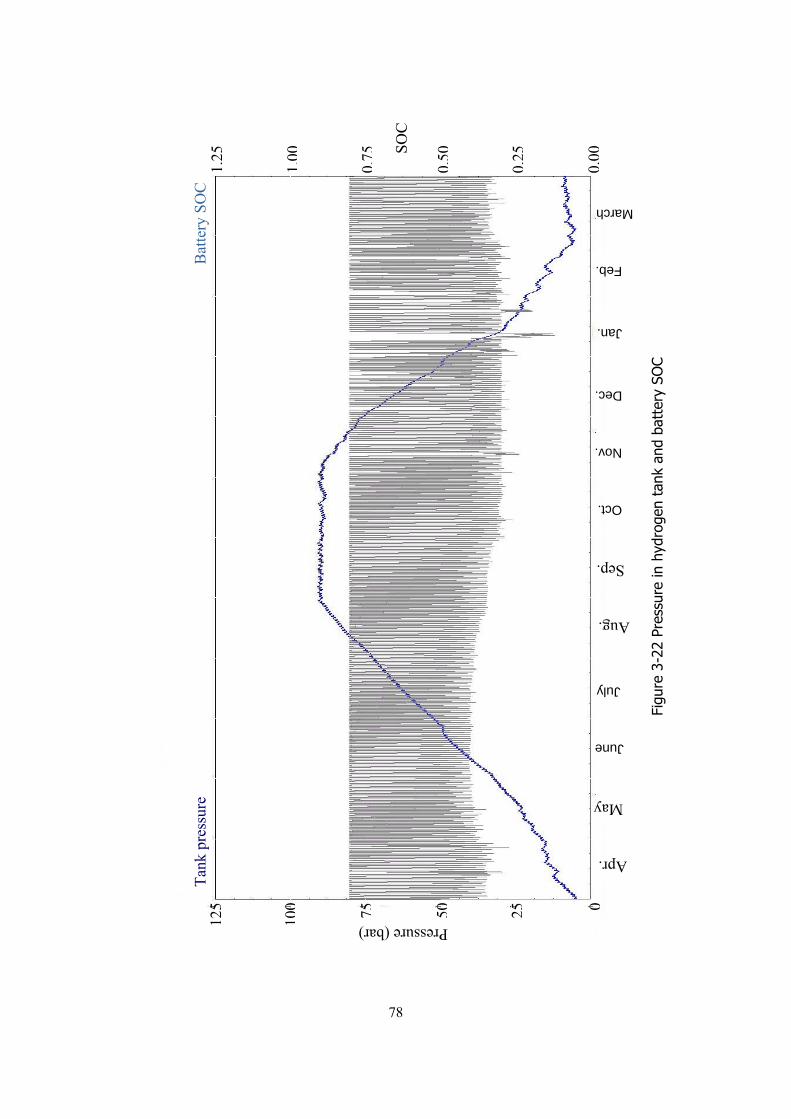
Figu

re 3

-22

Pres

sure

in h

ydro

gen

tank

and

bat

tery

SO

C

March

Feb.

May

Apr.

June

July

Aug.

Sep.

Oct.

Nov.

Dec.

Jan.

Tan

k pr

essu

re

Bat

tery

SO

C

1.25

1.00

0.75

0.50

0.25

0.00SO

C

125

100 75 50 25 0

Pressure (bar)

78

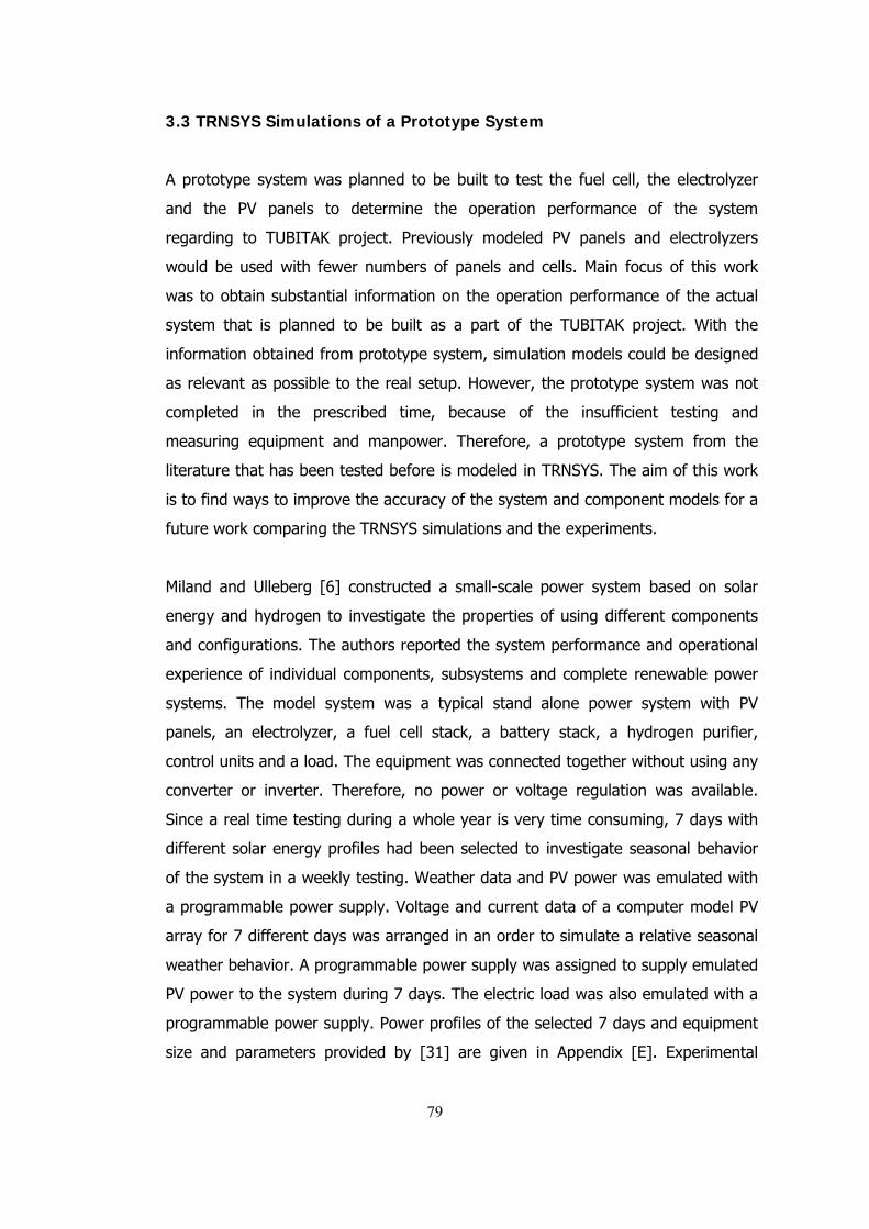
3.3 TRNSYS Simulations of a Prototype System

A prototype system was planned to be built to test the fuel cell, the electrolyzer

and the PV panels to determine the operation performance of the system

regarding to TUBITAK project. Previously modeled PV panels and electrolyzers

would be used with fewer numbers of panels and cells. Main focus of this work

was to obtain substantial information on the operation performance of the actual

system that is planned to be built as a part of the TUBITAK project. With the

information obtained from prototype system, simulation models could be designed

as relevant as possible to the real setup. However, the prototype system was not

completed in the prescribed time, because of the insufficient testing and

measuring equipment and manpower. Therefore, a prototype system from the

literature that has been tested before is modeled in TRNSYS. The aim of this work

is to find ways to improve the accuracy of the system and component models for a

future work comparing the TRNSYS simulations and the experiments.

Miland and Ulleberg [6] constructed a small-scale power system based on solar

energy and hydrogen to investigate the properties of using different components

and configurations. The authors reported the system performance and operational

experience of individual components, subsystems and complete renewable power

systems. The model system was a typical stand alone power system with PV

panels, an electrolyzer, a fuel cell stack, a battery stack, a hydrogen purifier,

control units and a load. The equipment was connected together without using any

converter or inverter. Therefore, no power or voltage regulation was available.

Since a real time testing during a whole year is very time consuming, 7 days with

different solar energy profiles had been selected to investigate seasonal behavior

of the system in a weekly testing. Weather data and PV power was emulated with

a programmable power supply. Voltage and current data of a computer model PV

array for 7 different days was arranged in an order to simulate a relative seasonal

weather behavior. A programmable power supply was assigned to supply emulated

PV power to the system during 7 days. The electric load was also emulated with a

programmable power supply. Power profiles of the selected 7 days and equipment

size and parameters provided by [31] are given in Appendix [E]. Experimental

79

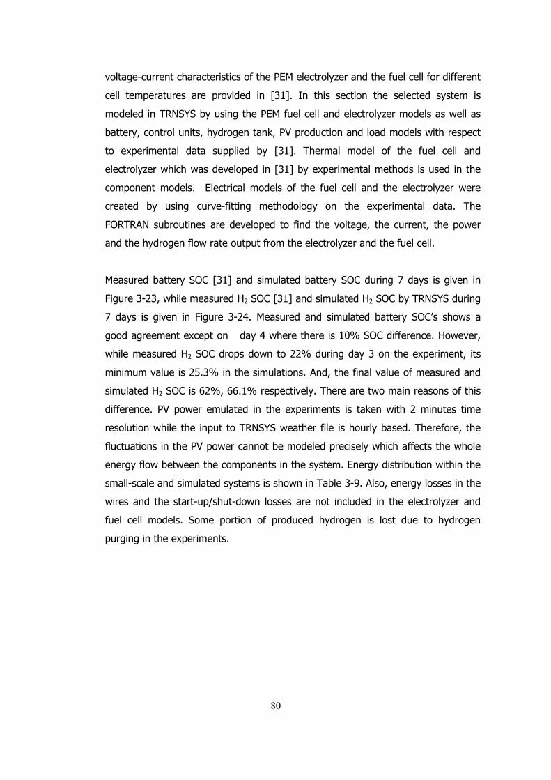
voltage-current characteristics of the PEM electrolyzer and the fuel cell for different

cell temperatures are provided in [31]. In this section the selected system is

modeled in TRNSYS by using the PEM fuel cell and electrolyzer models as well as

battery, control units, hydrogen tank, PV production and load models with respect

to experimental data supplied by [31]. Thermal model of the fuel cell and

electrolyzer which was developed in [31] by experimental methods is used in the

component models. Electrical models of the fuel cell and the electrolyzer were

created by using curve-fitting methodology on the experimental data. The

FORTRAN subroutines are developed to find the voltage, the current, the power

and the hydrogen flow rate output from the electrolyzer and the fuel cell.

Measured battery SOC [31] and simulated battery SOC during 7 days is given in

Figure 3-23, while measured H2 SOC [31] and simulated H2 SOC by TRNSYS during

7 days is given in Figure 3-24. Measured and simulated battery SOC’s shows a

good agreement except on day 4 where there is 10% SOC difference. However,

while measured H2 SOC drops down to 22% during day 3 on the experiment, its

minimum value is 25.3% in the simulations. And, the final value of measured and

simulated H2 SOC is 62%, 66.1% respectively. There are two main reasons of this

difference. PV power emulated in the experiments is taken with 2 minutes time

resolution while the input to TRNSYS weather file is hourly based. Therefore, the

fluctuations in the PV power cannot be modeled precisely which affects the whole

energy flow between the components in the system. Energy distribution within the

small-scale and simulated systems is shown in Table 3-9. Also, energy losses in the

wires and the start-up/shut-down losses are not included in the electrolyzer and

fuel cell models. Some portion of produced hydrogen is lost due to hydrogen

purging in the experiments.

80

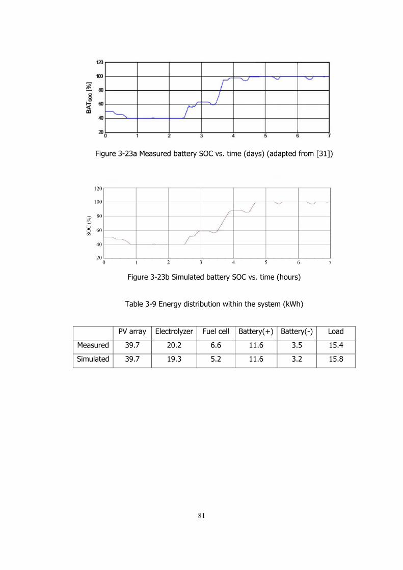
Figure 3-23a Measured battery SOC vs. time (days) (adapted from [31])

Figure 3-23b Simulated battery SOC vs. time (hours)

Table 3-9 Energy distribution within the system (kWh)

PV array Electrolyzer Fuel cell Battery(+) Battery(-) Load

Measured 39.7 20.2 6.6 11.6 3.5 15.4

Simulated 39.7 19.3 5.2 11.6 3.2 15.8

100

80

60

40

120

20

SO

C (

%)

0 1 2 3 4 5 6 7

81

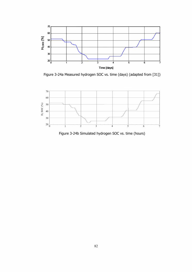
Figure 3-24a Measured hydrogen SOC vs. time (days) (adapted from [31])

Figure 3-24b Simulated hydrogen SOC vs. time (hours)

60

50

40

30

70

20

H2

SO

C (

%)

0 1 2 3 4 5 6 7

82

6 CHAPTER 4

CONCLUSIONS

4.1 Results

In this study, stand alone power systems are modeled and system parameters are

analyzed using a commercial software. The study is focused on the effects of

system components and on the total performance of the system. The photovoltaic

panels and the PEM electrolyzers are modeled individually using FORTRAN

subroutines. Numerical outputs of these components are compared with the

experimental results. The study shows how pressure in the hydrogen tank can be

used as a key system performance indicator, provided that no system constraints

are violated. The performance of the system can be significantly affected by the

small variations made on the system elements.

Hydrogen is the only energy storage for a Stand-Alone Power System without a

battery pack. The system is based on electricity-to-hydrogen and hydrogen-to-

electricity conversion which is an inefficient way of handling the extra energy.

Assembling PV panels with 50o surface slope reduces the amount of this

conversion and expected to increase the system performance and thus reduce the

size of the equipments used. However, PV panels produce 5% more energy if they

are assembled at 30o surface slope, and only 20% of this additional energy is lost

during the electricity-hydrogen conversions. Therefore, the system performance is

improved by installing the PV panels with 30o surface slope compared to the panels

with 50o surface slope. Assembling the PV panels in such a way that the surface

slope can be adjusted manually or automatically during the year develops the

system performance.

83

Increasing the number of electrolyzer cells adds additional initial cost to the system

but also increases the system efficiency and life time of the whole electrolyzer

stack.

Adding a battery pack plays an important role on the system performance and

efficiency as well as the size of other components in the system. Increasing the

number of batteries used also increases the system efficiency and decreases the

other component sizes. On the other hand, the cost of the battery pack increases

with a high rate while cost of other equipments decreases with a lesser rate.

Energy and power densities of lead-acid batteries are much lower than the

hydrogen tanks and the fuel cells. A 100 bar hydrogen tank can store 5 times more

energy than a battery pack having the same volume. The trade-offs between the

battery pack and the other components in the system should be examined

accurately.

Auxiliary equipment brings extra load on the system but they are essential for

steady and continuous operation of a stand-alone power system. If grid electricity

is not used for auxiliary equipment, a battery pack or a fuel cell stack working

continuously should provide energy to these equipment. Since the control panel

and similar equipment should work continuously.

4.2 Future Work

Typical Meteorological Year data is used in the system models. Since the weather

shows variations throughout the years, it is definite that there will be years with

lower solar energy available. The worst case scenarios should be taken into

account for the simulations and backup solutions should be considered such as

using grid power or extra hydrogen storage.

The load profile used in the simulations is constant for long hours, however the

actual load profile of an emergency service has power fluctuations and peak-

powers. Fuel cell performance is significantly affected by the load. The

performance of the fuel cell and thus the system will change if an actual load

84

profile is used. Control strategy of the fuel cell should be examined such as the

fuel cells can operate under constant power or variable power. Operating the fuel

cells under constant power and using batteries for the small fluctuations in the

load can perform better than operating the fuel cells under variable power. Also

batteries can be used for during peak-hours to reduce the load on the fuel cell

since the fuel cell efficiency drops as the load increases. Hydrogen leakage from

the connections and storage tank and electrical loses in the wires can be modeled

to improve numerical models.

A detailed life-time cost analysis for the modeled systems should be performed to

see the actual effects of the parameters. It is necessary to avoid the operating

schemes that reduce the life of the electrochemical equipment which are

electrolyzers, fuel cells and batteries. Therefore, other system parameters, such as

number of start-ups and stops of the fuel cells and electrolyzers, the amount of

time when these components are operating under high or low power levels, should

also be considered.

85

REFERENCES

[1] Renewable Energy Policy Network for the 21st Century, “Renewables 2007

Global Status Report”, 2007.

[2] Renewable Energy Policy Network for the 21st Century, “Renewables 2009

Global Status Report”, 2009.

[3] N. Gupta, G.F. Alapatt, R. Podila, R. Singh, K.F. Poole, “Prospects of

nanostructure-based solar cells for manufacturing future generations of

photovoltaic modules”, International Journal of Photoenergy, vol. 2009, id:

154059, 2009.

[4] TUBITAK Project no: 106G130 Project Proposal, 2006.

[5] P. Hollmuller, J.M. Joubert, B. Lachal, K. Yvon, “Evaluation of a 5kWp

photovoltaic hydrogen production and storage installation for a residential home in

Switzerland”, International Journal of Hydrogen Energy, vol. 25, pp. 97-109, 2000.

[6] H. Miland, O. Ulleberg, “Testing of a small-scale stand-alone power system

based on solar energy and hydrogen”, Solar Energy, In Press, Uncorrected Proof,

Available online (http://www.sciencedirect.com/science/article/B6V50-4SNPWJF-

1/2/4d362d10af5abe0bf1c5a1aaf22c3bea)

[7] J.P. Vanhanen, P.D. Lund, J.S. Tolonen, “Electrolyser-metal hydride-fuel cell

system for seasonal energy storage”, International Journal of Hydrogen Energy,

vol. 23, No 4, pp 267-271, 1998.

[8] S. Galli, M. Stefanoni, “Development of a Solar-hydrogen cycle in Italy”, Int. J.

Hydrogen Energy, vol 22, pp. 453-458, 1997.

86

[9] A.M. Chaparro, J. Soler, M.J. Escudero, E.M.L. de Ceballos, U. Wittstadt, L.

Daza, “Date results and operational experience with a solar hydrogen system”,

Journal of Power Sources, vol. 144, pp. 165-169, 2005.

[10] A. Sasitharanuwat, W. Rakwichian, N. Ketjoy, S. Yammen, “Performance

evaluation of a 10 kWp PV power system prototype for isolated building in

Thailand”, Renewable Energy, vol. 32, pp. 1288-1300, 2007.

[11] K. Agbossou, M. Kolhe, J. Hamelin, T.K. Bose, “Performance of a sand-aone

rnewable eergy sstem based on eergy storage as hydrogen”, IEEE Transactions on

Energy Conversion, vol. 19, pp. 633-640, 2004.

[12] D. Shapiro, J. Duffy, M. Kimble, M. Pien, “Solar-powered regenerative PEm

electrolyzer/fuel cell system”, Solar Energy, vol. 79, pp. 544-550, 2005.

[13] A.N. Kelly, L.T. Gibson, D.B. Ouwerkerk, “A solar-powered, high-efficiency

hydrogen fueling system using high pressure electrolysis of water: Design and

initial results” International Journal of Hydrogen Energy, vol.33, pp.2747-2764,

2008.

[14] O. Ulleberg, “Stand-alone power systems for the future: Optimal design,

operation & control of solar-hydrogen energy systems”, Ph.D. dissertation,

Norwegian University of Science and Technology Trondheim, Norway, 1998.

[15] O. Ulleberg, “The importance of control strategies in PV-hydrogen systems”,

Solar Energy, vol. 76, pp. 323-329, 2004.

[16] R. Dufo-Lopez, J.L. Bernal-Agustin, J. Contreras, “Optimization of Control

Strategies for Stand-Alone Renewable Energy Systems with Hydrogen Storage”,

Renewable Energy, vol. 32, pp. 1102-1126, 2007.

87

[17] M. Santarelli, M. Cali, S. Macagno, “Design and analysis of stand-alone

hydrogen systems with different renewable sources”, Internal Journal of Hydrogen

Energy, vol. 29, pp. 1571-1586, 2004.

[18] S. Pedrazzi, G. Sini, P. Tartarini, “Complete modeling and software

implementation of a virtual solar hydrogen hybrid system”, Energy Conversion and

Management, vol. 51, pp.122-129, 2010.

[19] J. Samaniego, F. Alija, S. Sanz, C. Valmaseda, F. Frechoso, “Economic and

technical analysis of a hybrid wind fuel cell energy system”, Renewable Energy,

vol. 33, pp. 839-845, 2008.

[20] S.S. Deshmukh, R.F. Boehm, “Reviews of modeling details revealed to

renewably powered hydrogen systems”, Renewable and Sustainable Energy

Reviews, vol. 12, pp. 2301-2330, 2007.

[21] D.B. Nelson, M.H. Nehrir, C. Wang, “Unit sizing and cost analysis of stand-

alone hybrid wind/PV/fuel cell power generation systems” Renewable Energy, vol.

31, pp. 1641-1656, 2006.

[22] O.C. Onar, M. Uzunoglu, M.S. Alam, “Dynamic modeling, design and

simulation of a wind/fuel cell/ultra-capacitor-based hybrid power generation

system”, Journal of Power Sources, vol. 161, pp. 707-722, 2006.

[23] O.C. Onar, M. Uzunoglu, M.S. Alam, “Modeling, control and simulation of a

PV/FC/UC based hybrid power generation system for stand-alone applications”,

Renewable Energy, vol. 34, pp. 509-520, 2009.

[24] D. Sera, R. Teodorescu, P. Rodriguez, “PV panel model based on datasheet

values”, Industrial Electronics, 2007. ISIE 2007. IEEE International Symposium, pp.

2392-2396, 2007.

88

[25] G. Vachtsevanos, K. Kalaitzakis, “A hybrid photovoltaic simulator for utility

interactive studies”, IEEE Power Engineering Society summer meeting, Mexico City,

1986.

[26] M. Mattei, G. Notton, C. Cristofari, M. Muselli, P. Poggi, “Calculation of a

polycrystalline PV module temperature using a simple method of energy balance”,

Renewable Energy, vol. 31, pp. 553-567, 2005.

[27] W.A. Beckman, W. Desoto, S.A. Klein, “Improvement and validation of a

model for photovoltaic array performance” Solar Energy, vol. 80, pp. 78-88, 2006.

[28] Nonlinear Regression and Curve fitting,

http://www.nlreg.com, last accessed at April 2010.

[29] N. Gupta, G.F. Alapatt, R. Podila, R. Singh, K.F. Poole, “Prospects of

nanostructure-based solar cells for manufacturing future generations of

photovoltaic modules”, International Journal of Photoenergy, vol. 2009, id:

154059, 2009.

[30] D.A. Bechrakis, E.J. McKeogh, P.D. Gallagher, “Simulation and operational

assessment for a small autonomous wind-hydrogen energy system”, Energy

Conversion and Management, vol. 47, pp. 46-59, 2006.

[31] H. Miland, “Operational experience and control strategies for a stand-alone

power system based on renewable energy and hydrogen”, Ph.D. dissertation,

Norwegian University of Science and Technology Trondheim, Norway, 2005.

[32] Model KC130TM data sheet, Kyocera Corporation.

89

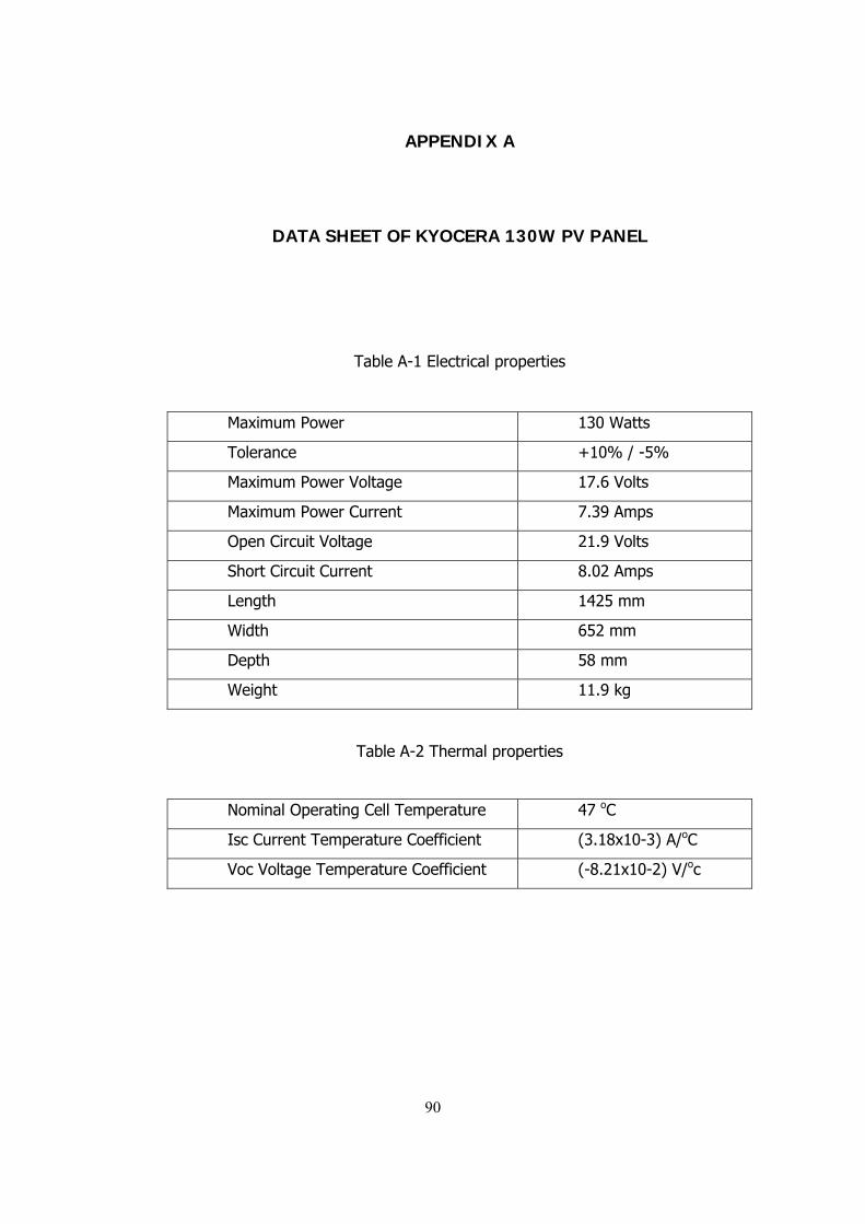
APPENDIX A

DATA SHEET OF KYOCERA 130W PV PANEL

Table A-1 Electrical properties

Maximum Power 130 Watts

Tolerance +10% / -5%

Maximum Power Voltage 17.6 Volts

Maximum Power Current 7.39 Amps

Open Circuit Voltage 21.9 Volts

Short Circuit Current 8.02 Amps

Length 1425 mm

Width 652 mm

Depth 58 mm

Weight 11.9 kg

Table A-2 Thermal properties

Nominal Operating Cell Temperature 47 oC

Isc Current Temperature Coefficient (3.18x10-3) A/oC

Voc Voltage Temperature Coefficient (-8.21x10-2) V/oc

90

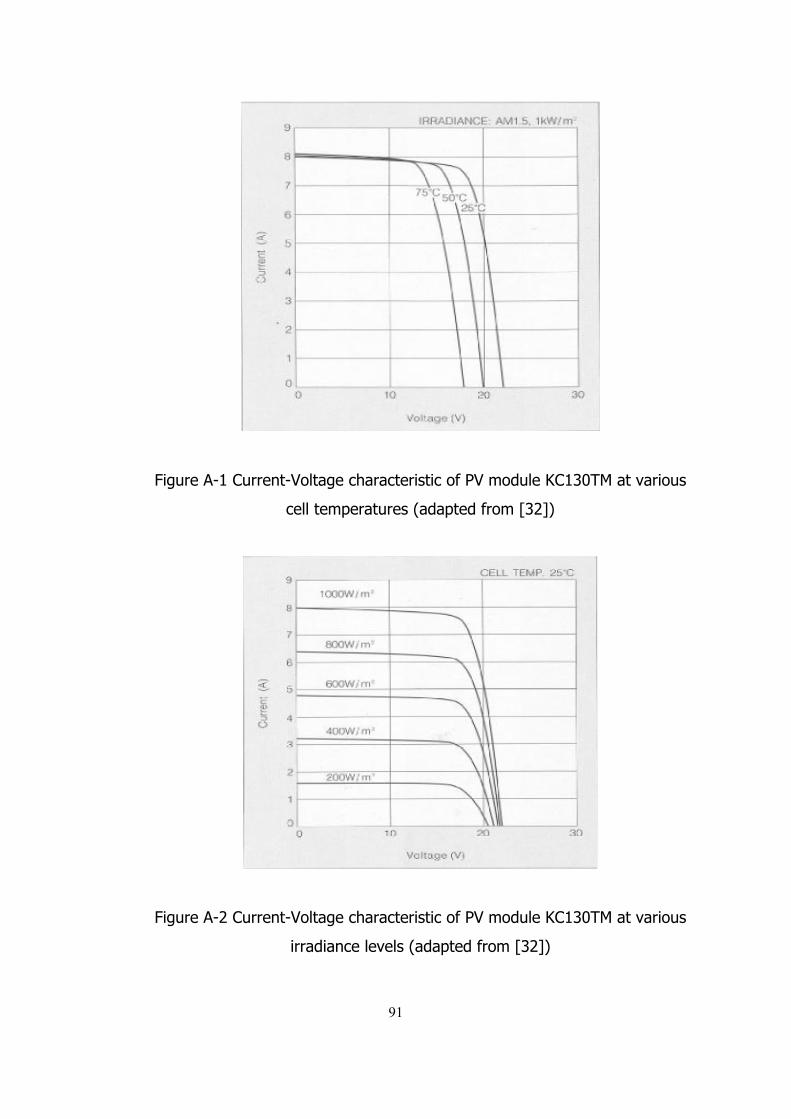
Figure A-1 Current-Voltage characteristic of PV module KC130TM at various

cell temperatures (adapted from [32])

Figure A-2 Current-Voltage characteristic of PV module KC130TM at various

irradiance levels (adapted from [32])

91

APPENDIX B

FORTRAN CODE OF PV PANEL MODEL

C Initial estimations for the PV parameters

Rs=0.8

Rsh=100

A=0.8

I0=0.00001

x(1)=Rs

x(2)=Rsh

x(3)=A

x(4)=I0

N=1

10 N=N+1

DO 15 i=1,4

xold(i)=x(i)

15 CONTINUE

u(1)=Iph-Isc-(x(4)*(exp((Isc*x(1))/(ns*Vt*x(3)))-1))-((Isc*x(1))/

.x(2))

u(2)=Iph-Impp-(x(4)*(exp((Vmpp+Impp*x(1))/(ns*x(3)*Vt))-1))-

.((Vmpp+Impp*x(1))/x(2))

u(3)=Iph-x(4)*(exp((Vmpp+Impp*x(1))/(x(3)*Vt*ns))-1)-((Vmpp+Impp*

.x(1))/x(2))-Vmpp*((1/x(2))+((x(4)*exp((Vmpp+Impp*x(1))/(x(3)*Vt*

.ns)))/(x(3)*Vt*ns)))

u(4)=Iph-(x(4)*(exp(Voc/(ns*Vt*x(3)))-1))-(Voc/x(2))

C partial derivatives of FIsc wrt. Rs, Rsh, A and I0 respectively

FIscdRs=-(Isc/Rsh)-((I0*Isc*exp((Isc*Rs)/(A*Vt*ns)))/(A*Vt*ns))

coef(1,1)=FIscdRs

FIscdRsh=(Isc*Rs)/(Rsh*Rsh)

coef(1,2)=FIscdRsh

FIscdA=(I0*Isc*Rs*exp((Isc*Rs)/(A*Vt*ns)))/(A*A*Vt*ns)

coef(1,3)=FIscdA

FIscdI0=1-exp((Isc*Rs)/(ns*Vt*A))

coef(1,4)=FIscdI0

C partial derivatives of FMpp wrt. Rs, Rsh, A and I0 respectively

FMppdRs=-(Impp/Rsh)-((I0*Impp*exp((Vmpp+Impp*Rs)/(A*Vt*ns)))/

.(A*Vt*ns))

coef(2,1)=FMppdRs

FMppdRsh=(Vmpp+Impp*Rs)/(Rsh*Rsh)

92

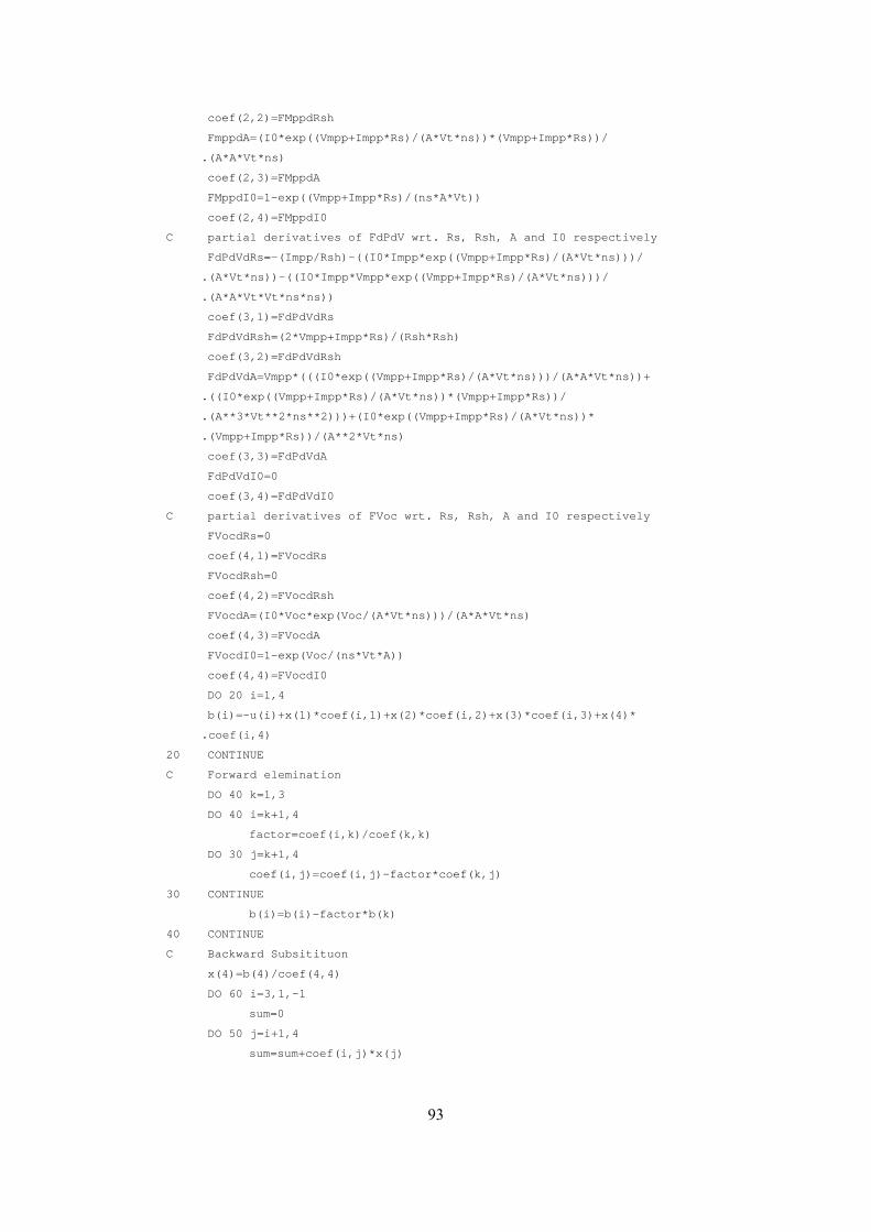
coef(2,2)=FMppdRsh

FmppdA=(I0*exp((Vmpp+Impp*Rs)/(A*Vt*ns))*(Vmpp+Impp*Rs))/

.(A*A*Vt*ns)

coef(2,3)=FMppdA

FMppdI0=1-exp((Vmpp+Impp*Rs)/(ns*A*Vt))

coef(2,4)=FMppdI0

C partial derivatives of FdPdV wrt. Rs, Rsh, A and I0 respectively

FdPdVdRs=-(Impp/Rsh)-((I0*Impp*exp((Vmpp+Impp*Rs)/(A*Vt*ns)))/

.(A*Vt*ns))-((I0*Impp*Vmpp*exp((Vmpp+Impp*Rs)/(A*Vt*ns)))/

.(A*A*Vt*Vt*ns*ns))

coef(3,1)=FdPdVdRs

FdPdVdRsh=(2*Vmpp+Impp*Rs)/(Rsh*Rsh)

coef(3,2)=FdPdVdRsh

FdPdVdA=Vmpp*(((I0*exp((Vmpp+Impp*Rs)/(A*Vt*ns)))/(A*A*Vt*ns))+

.((I0*exp((Vmpp+Impp*Rs)/(A*Vt*ns))*(Vmpp+Impp*Rs))/

.(A**3*Vt**2*ns**2)))+(I0*exp((Vmpp+Impp*Rs)/(A*Vt*ns))*

.(Vmpp+Impp*Rs))/(A**2*Vt*ns)

coef(3,3)=FdPdVdA

FdPdVdI0=0

coef(3,4)=FdPdVdI0

C partial derivatives of FVoc wrt. Rs, Rsh, A and I0 respectively

FVocdRs=0

coef(4,1)=FVocdRs

FVocdRsh=0

coef(4,2)=FVocdRsh

FVocdA=(I0*Voc*exp(Voc/(A*Vt*ns)))/(A*A*Vt*ns)

coef(4,3)=FVocdA

FVocdI0=1-exp(Voc/(ns*Vt*A))

coef(4,4)=FVocdI0

DO 20 i=1,4

b(i)=-u(i)+x(1)*coef(i,1)+x(2)*coef(i,2)+x(3)*coef(i,3)+x(4)*

.coef(i,4)

20 CONTINUE

C Forward elemination

DO 40 k=1,3

DO 40 i=k+1,4

factor=coef(i,k)/coef(k,k)

DO 30 j=k+1,4

coef(i,j)=coef(i,j)-factor*coef(k,j)

30 CONTINUE

b(i)=b(i)-factor*b(k)

40 CONTINUE

C Backward Subsitituon

x(4)=b(4)/coef(4,4)

DO 60 i=3,1,-1

sum=0

DO 50 j=i+1,4

sum=sum+coef(i,j)*x(j)

93

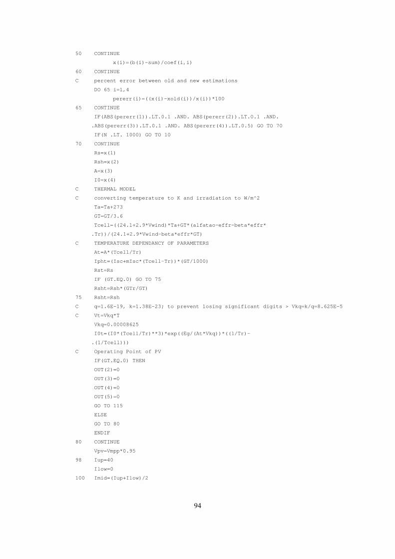
50 CONTINUE

x(i)=(b(i)-sum)/coef(i,i)

60 CONTINUE

C percent error between old and new estimations

DO 65 i=1,4

pererr(i)=((x(i)-xold(i))/x(i))*100

65 CONTINUE

IF(ABS(pererr(1)).LT.0.1 .AND. ABS(pererr(2)).LT.0.1 .AND.

.ABS(pererr(3)).LT.0.1 .AND. ABS(pererr(4)).LT.0.5) GO TO 70

IF(N .LT. 1000) GO TO 10

70 CONTINUE

Rs=x(1)

Rsh=x(2)

A=x(3)

I0=x(4)

C THERMAL MODEL

C converting temperature to K and irradiation to W/m^2

Ta=Ta+273

GT=GT/3.6

Tcell=((24.1+2.9*Vwind)*Ta+GT*(alfatao-effr-beta*effr*

.Tr))/(24.1+2.9*Vwind-beta*effr*GT)

C TEMPERATURE DEPENDANCY OF PARAMETERS

At=A*(Tcell/Tr)

Ipht=(Isc+mIsc*(Tcell-Tr))*(GT/1000)

Rst=Rs

IF (GT.EQ.0) GO TO 75

Rsht=Rsh*(GTr/GT)

75 Rsht=Rsh

C q=1.6E-19, k=1.38E-23; to prevent losing significant digits > Vkq=k/q=8.625E-5

C Vt=Vkq*T

Vkq=0.00008625

I0t=(I0*(Tcell/Tr)**3)*exp((Eg/(At*Vkq))*((1/Tr)-

.(1/Tcell)))

C Operating Point of PV

IF(GT.EQ.0) THEN

OUT(2)=0

OUT(3)=0

OUT(4)=0

OUT(5)=0

GO TO 115

ELSE

GO TO 80

ENDIF

80 CONTINUE

Vpv=Vmpp*0.95

98 Iup=40

Ilow=0

100 Imid=(Iup+Ilow)/2

94

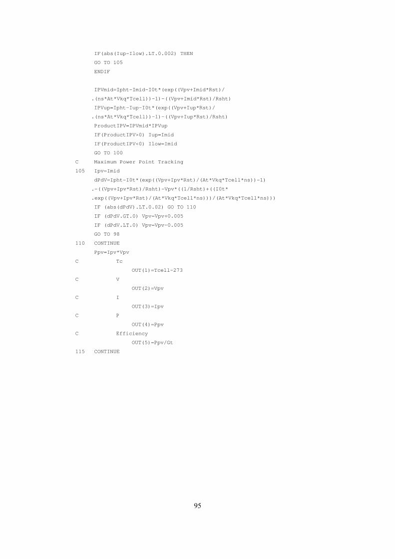
IF(abs(Iup-Ilow).LT.0.002) THEN

GO TO 105

ENDIF

IPVmid=Ipht-Imid-I0t*(exp((Vpv+Imid*Rst)/

.(ns*At*Vkq*Tcell))-1)-((Vpv+Imid*Rst)/Rsht)

IPVup=Ipht-Iup-I0t*(exp((Vpv+Iup*Rst)/

.(ns*At*Vkq*Tcell))-1)-((Vpv+Iup*Rst)/Rsht)

ProductIPV=IPVmid*IPVup

IF(ProductIPV>0) Iup=Imid

IF(ProductIPV<0) Ilow=Imid

GO TO 100

C Maximum Power Point Tracking

105 Ipv=Imid

dPdV=Ipht-I0t*(exp((Vpv+Ipv*Rst)/(At*Vkq*Tcell*ns))-1)

.-((Vpv+Ipv*Rst)/Rsht)-Vpv*((1/Rsht)+((I0t*

.exp((Vpv+Ipv*Rst)/(At*Vkq*Tcell*ns)))/(At*Vkq*Tcell*ns)))

IF (abs(dPdV).LT.0.02) GO TO 110

IF (dPdV.GT.0) Vpv=Vpv+0.005

IF (dPdV.LT.0) Vpv=Vpv-0.005

GO TO 98

110 CONTINUE

Ppv=Ipv*Vpv

C Tc

OUT(1)=Tcell-273

C V

OUT(2)=Vpv

C I

OUT(3)=Ipv

C P

OUT(4)=Ppv

C Efficiency

OUT(5)=Ppv/Gt

115 CONTINUE

95

APPENDIX C

FORTRAN CODE OF PEM ELECTROLYZER MODEL

C Calculating maximum power that can electrolyzer work at

Tmax=Tmax+273

Pmin=25*ns

Tambient=20

10 Iup=200

Ilow=0

15 Imid=(Iup+Ilow)/2

IF(abs(Iup-Ilow).LT.0.000001) THEN

GO TO 20

ENDIF

Ielemid=(A*(Ioa*Tmax+Iob)*(exp(((1-alfa)*n*F*(Vcell-Veq))/

. (R*Tmax))-exp(((-alfa)*n*F*(Vcell-Veq))/(R*Tmax))))-Imid

Ieleup=(A*(Ioa*Tmax+Iob)*(exp(((1-alfa)*n*F*(Vcell-Veq))/

. (R*Tmax))-exp(((-alfa)*n*F*(Vcell-Veq))/(R*Tmax))))-Iup

ProductIele=Ielemid*Ieleup

IF(ProductIele>0) Iup=Imid

IF(ProductIele<0) Ilow=Imid

GO TO 15

20 CONTINUE

Imax=Imid

Pmaxcell=Imax*Vcell

Pmaxele=Pmaxcell*ns*npmax

Pwasted=Pmaxele-Pele

IF(Pwasted>0) Pwasted=0

IF(Pele>Pmaxele) Pele=Pmaxele

IF(Pele.LT.Pmin) THEN

Pele=0

Ic=0

Tcell=Tambient

Efficiency=0

Vh2actual=0

npar=0

GO TO 60

ELSE

CONTINUE

96

END IF

C Calculating the optimum number of parallel electrolyzer stacks that would make

the electrolyzer work as close as possible to reference cell temperature

25 Iup=200

Ilow=0

30 Imid=(Iup+Ilow)/2

IF(abs(Iup-Ilow).LT.0.000001) THEN

GO TO 35

ENDIF

Ielemid=(A*(Ioa*Tcref+Iob)*(exp(((1-alfa)*n*F*(Vcell-Veq))/

. (R*Tcref))-exp(((-alfa)*n*F*(Vcell-Veq))/(R*Tcref))))-Imid

Ieleup=(A*(Ioa*Tcref+Iob)*(exp(((1-alfa)*n*F*(Vcell-Veq))/

. (R*Tcref))-exp(((-alfa)*n*F*(Vcell-Veq))/(R*Tcref))))-Iup

ProductIele2=Ielemid*Ieleup

IF(ProductIele2>0) Iup=Imid

IF(ProductIele2<0) Ilow=Imid

GO TO 30

35 CONTINUE

Ic=Imid

nstack=Pele/((Ic*Vcell)*ns)

npar=NINT(nstack)

IF(npar.GT.npmax) npar=npmax

Pc=Pele/(ns*npar)

Ic=Pc/Vcell

C Calculating cell temperature for given stack number

40 Tup=1000

Tlow=200

45 Tmid=(Tup+Tlow)/2

IF(abs(Tup-Tlow).LT.0.000001) THEN

GO TO 50

ENDIF

Telemid=(A*(Ioa*Tmid+Iob)*(exp(((1-alfa)*n*F*(Vcell-Veq))/

. (R*Tmid))-exp(((-alfa)*n*F*(Vcell-Veq))/(R*Tmid))))-Ic

Teleup=(A*(Ioa*Tup+Iob)*(exp(((1-alfa)*n*F*(Vcell-Veq))/

. (R*Tup))-exp(((-alfa)*n*F*(Vcell-Veq))/(R*Tup))))-Ic

ProductTele=Telemid*Teleup

IF(ProductTele>0) Tup=Tmid

IF(ProductTele<0) Tlow=Tmid

GO TO 45

50 CONTINUE

Tcell=Tmid-273

Tstan=0

Nh2ideal=ns*npar*(Ic/(2*F))

Vh2ideal=(Nh2ideal*R*(Tstan+273)*3600)/100000

Vh2actual=Vh2ideal*Feff

97

Efficiency=Vtn/Vcell

60 CONTINUE

C Pused

OUT(1)=Pele

C Iele

OUT(2)=Ic*npar

C Tc

OUT(3)=Tcell

C Efficiency

OUT(4)=Efficiency

C Vh2

OUT(5)=Vh2actual

C np

OUT(6)=npar

C Vo2

OUT(7)=Vh2actual/2

C-----------------------------------------------------------------------------------

------------------------------------

C EVERYTHING IS DONE - RETURN FROM THIS SUBROUTINE AND MOVE ON

RETURN 1

END

98

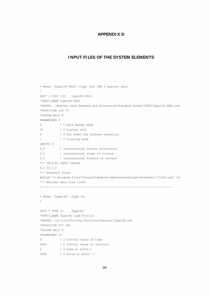
APPENDIX D

INPUT FILES OF THE SYSTEM ELEMENTS

* Model "Type109-TMY2" (Type 109) TMY 2 weather data

*

UNIT 3 TYPE 109 Type109-TMY2

*$UNIT_NAME Type109-TMY2

*$MODEL .\Weather Data Reading and Processing\Standard Format\TMY2\Type109-TMY2.tmf

*$POSITION 148 72

*$LAYER Main #

PARAMETERS 4

2 ! 1 Data Reader Mode

34 ! 2 Logical unit

4 ! 3 Sky model for diffuse radiation

1 ! 4 Tracking mode

INPUTS 3

0,0 ! [unconnected] Ground reflectance

0,0 ! [unconnected] Slope of surface

0,0 ! [unconnected] Azimuth of surface

*** INITIAL INPUT VALUES

0.2 30 0.0

*** External files

ASSIGN "C:\Program Files\Trnsys16\Weather\Meteonorm\Europe\TR-Ankara-171300.tm2" 34

*|? Weather data file |1000

*------------------------------------------------------------------------------

* Model "Type14h" (Type 14)

*

UNIT 7 TYPE 14 Type14h

*$UNIT_NAME Type14h Load Profile

*$MODEL .\Utility\Forcing Functions\General\Type14h.tmf

*$POSITION 247 245

*$LAYER Main #

PARAMETERS 10

0 ! 1 Initial value of time

2000 ! 2 Initial value of function

6 ! 3 Time at point-1

2000 ! 4 Value at point -1

99

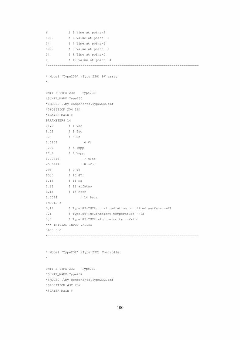
6 ! 5 Time at point-2

5000 ! 6 Value at point -2

24 ! 7 Time at point-3

5000 ! 8 Value at point -3

24 ! 9 Time at point-4

0 ! 10 Value at point -4

*------------------------------------------------------------------------------

* Model "Type230" (Type 230) PV array

*

UNIT 5 TYPE 230 Type230

*$UNIT_NAME Type230

*$MODEL .\My components\Type230.tmf

*$POSITION 254 164

*$LAYER Main #

PARAMETERS 14

21.9 ! 1 Voc

8.02 ! 2 Isc

72 ! 3 Ns

0.0259 ! 4 Vt

7.36 ! 5 Impp

17.6 ! 6 Vmpp

0.00318 ! 7 mIsc

-0.0821 ! 8 mVoc

298 ! 9 Tr

1000 ! 10 GTr

1.16 ! 11 Eg

0.81 ! 12 alfatao

0.16 ! 13 effr

0.0044 ! 14 Beta

INPUTS 3

3,18 ! Type109-TMY2:total radiation on tilted surface ->GT

3,1 ! Type109-TMY2:Ambient temperature ->Ta

3,3 ! Type109-TMY2:wind velocity ->Vwind

*** INITIAL INPUT VALUES

3600 0 0

*------------------------------------------------------------------------------

* Model "Type232" (Type 232) Controller

*

UNIT 2 TYPE 232 Type232

*$UNIT_NAME Type232

*$MODEL .\My components\Type232.tmf

*$POSITION 432 292

*$LAYER Main #

100

PARAMETERS 11

0 ! 1 PfcMin

5200 ! 2 PfcMax

4000 ! 3 PfcNom

0 ! 4 PeleMin

40000 ! 5 PeleMax

0.9 ! 6 SOCmax

0.2 ! 7 SOCmin

0.2 ! 8 SOCfclimit

0.95 ! 9 PLEVup

0.9 ! 10 PLEVlow

0.90 ! 11 InverterEff

INPUTS 4

Pout ! Equa:Pout ->Ppv

7,1 ! Type14h:Average value of function ->Pload

0,0 ! [unconnected] SOC

12,3 ! Type164a:PLEV ->PLEV

*** INITIAL INPUT VALUES

0 10000 0.95 0.9

*------------------------------------------------------------------------------

* Model "Type48a" (Type 48) Inverter

*

UNIT 10 TYPE 48 Type48a

*$UNIT_NAME Type48a

*$MODEL .\Electrical\Regulators and Inverters\System w_o battery storage\Type48a.tmf

*$POSITION 390 566

*$LAYER Main #

PARAMETERS 2

0 ! 1 Mode

0.95 ! 2 Efficiency

INPUTS 2

8,1 ! Type170f:P_FC ->Input power

7,1 ! Type14h:Average value of function ->Load power

*------------------------------------------------------------------------------

* Model "Type170f" (Type 170) Fuel Cell

*

UNIT 8 TYPE 170 Type170f

*$UNIT_NAME Type170f

*$MODEL .\Hydrogen Systems\Fuel Cells\PEMFC\Air-H2\TMODE=2\RTCTMODE=3\Type170f.tmf

*$POSITION 390 449

*$LAYER Main #

*$# OXMODE=1. Air on the cathode side.

*$# TMODE=2. TSTACK is calculated

101

*$# RTCTMODE=3. User supplied R_t & C_t values

PARAMETERS 12

1 ! 1 OXMODE

2 ! 2 TMODE

85 ! 3 NCELLS

1 ! 4 NSTACKS

260 ! 5 A_PEM

0.0118 ! 6 T_PEM

0.0 ! 7 GAMMA

0.7 ! 8 UC_MIN

700 ! 9 IC_MAX

3 ! 10 RTCTMODE

0.06179 ! 11 Rt

32197 ! 12 Ct

INPUTS 11

2,5 ! Type232:FCswitch ->SWITCH

11,2 ! Type175a-2:Iout ->IFC

0,0 ! [unconnected] TSTACKin

0,0 ! [unconnected] p_H2_in

0,0 ! [unconnected] p_O2_in

0,0 ! [unconnected] S_H2

0,0 ! [unconnected] S_O2

0,0 ! [unconnected] Tamb

0,0 ! [unconnected] TCWin

0,0 ! [unconnected] DELTATCW

0,0 ! [unconnected] Xevap

*** INITIAL INPUT VALUES

1 160 70 3 3 1.15 2.5 20 30 20 0.25

*------------------------------------------------------------------------------

* Model "Type175a-2" (Type 175)

*

UNIT 11 TYPE 175 Type175a-2 Power Conditioner

*$UNIT_NAME Type175a-2

*$MODEL .\Electrical\Power Conditioning\Power INPUT is known\Type175a.tmf

*$POSITION 339 366

*$LAYER Main #

*$# MODE=1. Input power (power source) is known.

PARAMETERS 7

1 ! 1 Mode

10000 ! 2 Pn

0 ! 3 P0Pn

2.06 ! 4 Us

50 ! 5 RiPn

1 ! 6 MP

0 ! 7 Paux

INPUTS 3

102

8,2 ! Type170f:Ustack ->Uin

8,2 ! Type170f:Ustack ->Uout_set

2,1 ! Type232:Pfc ->P

*** INITIAL INPUT VALUES

22E3 135 0

*------------------------------------------------------------------------------

* Model "Type231" (Type 231) Electrolyzer

*

UNIT 13 TYPE 231 Type231

*$UNIT_NAME Type231

*$MODEL .\My components\Type231.tmf

*$POSITION 701 196

*$LAYER Main #

PARAMETERS 14

0.0025 ! 1 A

50 ! 2 ns

15 ! 3 npmax

1.482 ! 4 Veq

0.97092 ! 5 alfa

68.572 ! 6 Ioa

-19242.33 ! 7 Iob

2 ! 8 n

96485.34 ! 9 F

8.314472 ! 10 R

323 ! 11 Tcref

80 ! 12 Tmax

0.95 ! 13 Feff

20 ! 14 Pressure

INPUTS 2

0,0 ! [unconnected] Vcell

2,2 ! Type232:Pele ->Pele

*** INITIAL INPUT VALUES

2 0

*------------------------------------------------------------------------------

* Model "Type164a" (Type 164) Hydrogen tank

*

UNIT 12 TYPE 164 Type164a

*$UNIT_NAME Type164a

*$MODEL .\Hydrogen Systems\Compressed Gas Storage\Hydrogen\Ideal Gas\Type164a.tmf

*$POSITION 659 449

*$LAYER Main #

*$# PMODE=1. Ideal Gas.

PARAMETERS 4

1 ! 1 PMODE

103

100 ! 2 PMAX

35 ! 3 VOL

2.016 ! 4 MOLAR

INPUTS 4

13,5 ! Type231:Vh2 ->VDOT_IN

8,6 ! Type170f:V_H2 ->VDOT_OUT

0,0 ! [unconnected] TGAS

0,0 ! [unconnected] PLEV_INI

*** INITIAL INPUT VALUES

0 0 20 0.05

*------------------------------------------------------------------------------

END

104

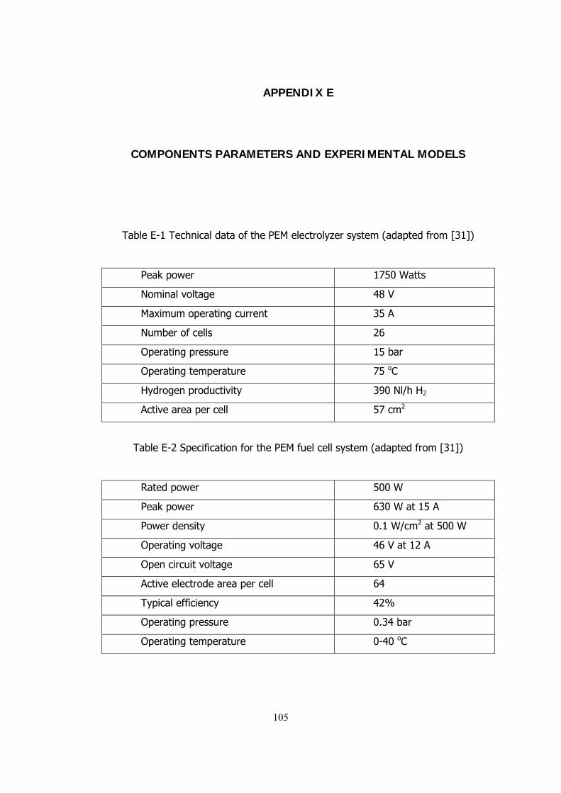
APPENDIX E

COMPONENTS PARAMETERS AND EXPERIMENTAL MODELS

Table E-1 Technical data of the PEM electrolyzer system (adapted from [31])

Peak power 1750 Watts

Nominal voltage 48 V

Maximum operating current 35 A

Number of cells 26

Operating pressure 15 bar

Operating temperature 75 oC

Hydrogen productivity 390 Nl/h H2

Active area per cell 57 cm2

Table E-2 Specification for the PEM fuel cell system (adapted from [31])

Rated power 500 W

Peak power 630 W at 15 A

Power density 0.1 W/cm2 at 500 W

Operating voltage 46 V at 12 A

Open circuit voltage 65 V

Active electrode area per cell 64

Typical efficiency 42%

Operating pressure 0.34 bar

Operating temperature 0-40 oC

105

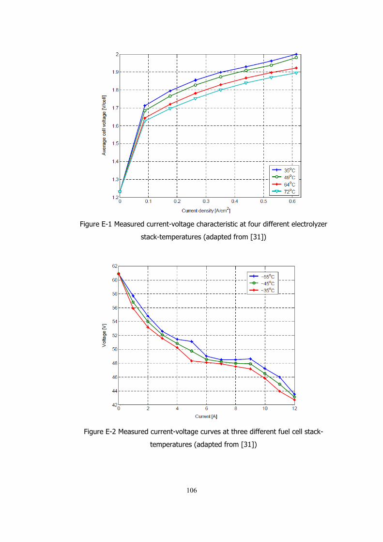
Figure E-1 Measured current-voltage characteristic at four different electrolyzer

stack-temperatures (adapted from [31])

Figure E-2 Measured current-voltage curves at three different fuel cell stack-

temperatures (adapted from [31])

106

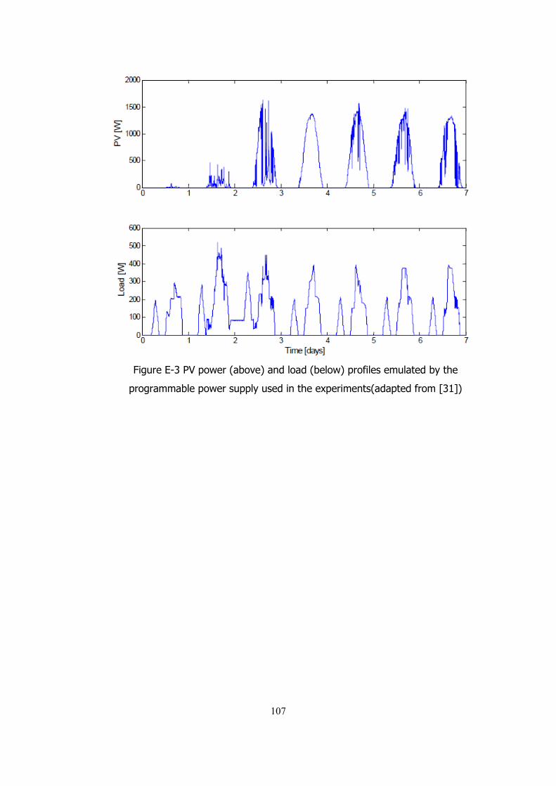
Figure E-3 PV power (above) and load (below) profiles emulated by the

programmable power supply used in the experiments(adapted from [31])

107