Embed Size (px)
Citation preview

ME 555 – DESIGN OPTIMIZATION COURSE UNDER THE INVALUABLE GUIDANCE OF PROF. MICHAEL KOKKOLARAS, UNIVERSITY OF MICHIGAN, ANN ARBOR
Solar Car System Optimization
Final Report
Team 6: Chiao-Ting Li, Yogita Pai, Zhenzhong Jia
4/14/2008
ABSTRACT: This paper formulates the optimization of a solar car based on UM Solar Car Team’s
Continuum. For this study three subsystems have been defined. These subsystems were modeled
independently. The first subsystem is the solar array/battery subsystem. The objective of this subsystem
is to maximize the nominal power production with the primary constraints being on the area of solar
cells, upper cover surface of Continuum. The second subsystem, models the long term racing strategy
for the solar car. The long term strategy will utilize the battery as energy buffer and determine cruise
speeds for each predefined route segment to minimize total racing time. The third subsystem, models
the short term racing strategy for the solar car. The short term strategy aims at optimizing the driving
strategy in order to minimize the total amount of energy required to travel over a hill and stop-n-go a
traffic signal. Based on the reference cruise speed taken from the long term strategy, the velocities,
acceleration and deceleration distances will be optimized.

2
Acknowledgement
The objective of this project was to develop a racing strategy for the solar car. A strategy is a
long-term plan of action designed to achieve a particular goal, most often a “winning” goal. We
treated this “strategy” as a design problem. Time based mathematical models were created for all
the subsystems and computational results obtained. These results obtained through optimization
were found to be fairly realistic.
Our involvement in this project has been one of the most significant academic challenges we
have ever had to face. Without the support, patience and guidance of the following people and
the team, this study would not have been completed. It is to them that we owe our deepest
gratitude.
We sincerely thank the UM solar car team for providing us with useful insight into this
project. We sincerely hope that our optimization study will benefit the team.
GSI Jarod Kelly who undertook to guide us despite his many other academic and
professional commitment. His wisdom, knowledge and commitment to the highest standard
inspired and motivated us.
Prof. Michael Kokkolaras for giving us an opportunity to work on this project and providing
all the encouragement and profound understanding.
Thanks is too mild a word to express our profound gratitude; however, the least we can say is
Thank you, Jarod and Prof. Kokkolaras.

3
Table of contents
1. Introduction…………………………………………………………………………………….7
SUBSYSTEM 1: SOLAR ARRAY OPTIMIZATION……………………………………......11
2.1 Problem Statement………………………………………..............…...………...…………...11
2.2 Modeling……………………………...………………………………...…………...……….12
2.2.1 Design Objective Simplification…..…...……………..……………...…...………..12
2.2.2 Identify the design variables and parameters…...……….….………..…...………..14
2. 2.3 Pre-processing of the original data.………………………......……....…...………15
2.2.4 Normal direction and area of each quad.………….………………….…...……….16
2.2.5 Update the quad_marker matrix to implement a specified design…...…...………..18
2.2.6 Energy production Calculation.…………………….…………….…..…...……….20
2.3 Meta-model Construction and Numerical Calculating.………………………...…...……….23
2.4 Mathematical Model and Summary Model.…………………………………...…...………..27
2.5 Model Analysis.…………………………………...………………………………...……….29
2.6 Summary and Discussion.…………………………………….………………...…...……….29
SUBSYSTEM 2: LONG TERM STRATEGY OPTIMIZATION OF A SOLAR CAR…….31
3.1 Problem statement……………………………………………………………………………32
3.2 Nomenclature………………………………………………………………………………...33
3.3 Mathematical models…………………………………………………………………….…..34
3.3.1 Assumptions…………………………………………………………………….….34
3.3.2 Route partition………………………………………………………………….….34
3.3.3 True model…………………………………………………………………………35
3.3.3.1 Vehicle model……………………………………………………………35

4
3.3.3.2 Array model……………………………………………………………...36
3.3.4 Metamodel…………………………………………………………………………38
3.3.4.1 Sunrise/Sunset charging curve fits……………………………………….38
3.3.4.2 Running/pull-in charging surface fits……………………………………40
3.3.4.3 Battery remnant…………………………………………………………..42
3.3.4.4 Metamodel validation……………………………………………………44
3.3.5 Objective function…………………………………………………………………45
3.3.6 Design variables and parameters…………………………………………………..46
3.3.7 Constraints…………………………………………………………………………47
3.4 Summary model……………………………………………………………………………...47
3.5 Model analysis……………………………………………………………………………….49
3.5.1 Equality constraints………………………………………………………………...49
3.5.2 Constraint redundancy……………………………………………………………..49
3.5.3 Feasible Set………………………………………………………………………...49
3.5.4 Monotonicity……………………………………………………………………….50
3.5.5 Well-boundedness………………………………………………………………….50
2.5.6 Model Simplification………………………………………………………………51
3.6 Numerical results…………………………………………………………………………….51
3.6.1 Unbounded variable………………………………………………………………..51
3.6.2 Released constraints………………………………………………………………..52
3.6.3 Constrained optimization…………………………………………………………..53
3.7 Parametric study……………………………………………………………………………...54
3.7.1 Vehicle weight (mass) ……………………………………………………………..54

5
3.7.2 Array max power…………………………………………………………………...55
3.7.3 Battery capacity……………………………………………………………………57
3.7.4 Initial battery remnant……………………………………………………………...58
3.7.5 Parametric interim conclusion……………………………………………………..59
3.8 Discussion…………………………………………………………………………………....59
3.8.1 Model-wise discussion…………………………………………………………….59
3.8.2 Race-wise discussion………………………………………………………………61
SUBSYSTEM 3: SHORT TERM STRATEGY OPTIMIZATION OF A SOLAR CAR…...63
4.1 Problem statement…………………………………………………………………………....63
4.2 Nomenclature………………………………………………………………………………...64
4.3 Mathematical Model………………………………………………………………………....65
4.3.1 Objective function…………………………………………………………………65
4.3.2 Constraints………………………………………………………………………....67
4.3.3 Design variables and Parameters…………………………………………………..69
4.3.4 Model summary…………………………………………………………………....70
4.3.5 Model analysis……………………………………………………………………..71
4.4 Hill scenario……...…………………………………………………………………………..71
4.4.1 Optimization study………………………………………………………………...71
4.4.1.1 Discretization…………………………………………………………….71
4.4.1.2 Metamodel generation…………………………………………………...72
4.4.1.3 Matlab fmincon Optimization results……………………………………74
4.4.2 Parametric study…………………………………………………………………....77
4.5 Stop-n-Go a traffic signal scenario…………………………………………………………..80

6
4.5.1 Optimization study…………………………………………………………………80
4.5.2 Parametric study…………………………………………………………………....81
4.6 Discussion of results………………………………………………………………………....85
SYSTEM INTEGRATION…………………………………………………………………….86
5.1 Integration Architecture……………………………………………………………………...86
5.2 Nomenclature………………………………………………………………………………...87
5.3 Mathematical model………………………………………………………………………….87
5.3.1 Array model simplification………………………………………………………...87
5.3.2 Integration of long term and short term running…………………………………...90
5.3.3 Model summary……………………………………………………………………93
5.3.4 Model analysis……………………………………………………………………..93
5.3.4.1 Monotonicity analysis……………………………………………………93
5.4 Numerical results…………………………………………………………………………….94
5.5 Parametric study……………………………………………………………………………...95
References………………………………………………………………………………………100
7
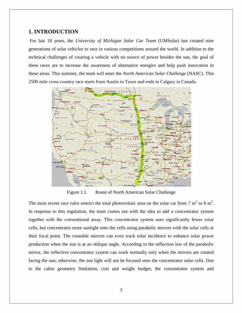
1. INTRODUCTION
For last 18 years, the University of Michigan Solar Car Team (UMSolar) has created nine
generations of solar vehicles to race in various competitions around the world. In addition to the
technical challenges of creating a vehicle with no source of power besides the sun, the goal of
these races are to increase the awareness of alternative energies and help push innovation in
these areas. This summer, the team will enter the North American Solar Challenge (NASC). This
2500 mile cross country race starts from Austin in Taxes and ends in Calgary in Canada.
Figure 1.1. Route of North American Solar Challenge
The most recent race rules restrict the total photovoltaic area on the solar car from 7 m2 to 6 m
2.
In response to this regulation, the team comes out with the idea to add a concentrator system
together with the conventional array. This concentrator system uses significantly fewer solar
cells, but concentrates more sunlight onto the cells using parabolic mirrors with the solar cells at
their focal point. The rotatable mirrors can even track solar incidence to enhance solar power
production when the sun is at an oblique angle. According to the reflection law of the parabolic
mirror, the reflective concentrator system can work normally only when the mirrors are rotated
facing the sun; otherwise, the sun light will not be focused onto the concentrator solar cells. Due
to the cabin geometry limitation, cost and weight budget, the concentrator system and

8
conventional arrays will coexist on the solar car. Here comes the opportunity to optimize the
layout of the solar cells for the 2008 North American Solar Challenge (NASC 2008).
Figure 1.2. The solar car, Continuum, 07‟-08‟ generation
For the 2500-mile long race route, the best team can finish it in four days while a new team
might end up by more than ten days. The total energy used is 80kWh~120kWh. So the pre-
charged 5kWh in the battery is nowhere enough to finish the race. (The race rules restrict the
battery capacity to be less than 5kWh). However the battery is a crucial component in viewpoint
of strategy; it serves as an energy buffer. At noon, the sun will provide excessive power to drive
the solar car. The surplus power will be charged into the battery for later use. In early morning
and late afternoon, the solar car will run on both solar power and battery power. The long term
race strategy aims to provide average cruising speed over a long distance by manipulating the
battery remnant to compromise the solar radiation variation due to sunrise and sunset. The
alternate goal is to run as fast as possible to win the trophy. Hence it would be beneficial to drain
out every watt when arriving at the finish line. While this problem is more like a decision making
process, we tried to interpret it as a design problem that is to determine daily battery remnant and
overall average speed to minimize total race time.
Figure 1.3. The battery is located behind the driver

9
The solar races are on the public expressways .Territory undulation, stop signs and traffic signals
are expected frequently. Under these circumstances, the solar car will not be able to run at the
cruising speed derived from long term strategy. Also potential energy due to altitude difference
could be utilized to coast down the hill without using any power. Other studies indicate that it is
possible to take advantage from the stop-and-go driving and hill ascending/descending by
adjusting speed in advance and resuming back to original cruising speed after passing such
traffic event.
In conclusion, we formulate the solar car problem in two senses: power production, and power
consumption. The first subsystem (solar array optimization), will try to optimize the solar car
power income. The second subsystem (long term race strategy optimization), and the third
subsystem (short term race strategy optimization), will deal with the utilization of such
limited solar power to finish the race. The trade-offs among the three subsystems are weight,
energy available and speed. The increase in weight due to concentrator system for more power
production will harm the long term speed performance and short term hill climbing capability.
The long term battery scheduling may be limited by the solar array production and battery
capacity. We will try to integrate the three subsystems while considering weight, battery and
speed at one time.
Solar Array
Long Term Strategy
Vcruise
Short Term Strategy
Energy/weight
Weight
Minimum Run Time
Solar Angle
Vehicle Parameters
Route Conditions
Race Rules etc.
Figure 1.4. Three subsystem overview
10
Today, a typical competitive solar car can finish its race with an average speed around 90 km/h
in the World Solar Challenge (WSC). For the North American Solar Challenge, this value will be
smaller due to the relatively less solar irradiation and rough terrain (UM‟s Momentum finished
the challenge at an average speed of 74.4 km/h as the champion in the nearest 2005 NASC
competition).
Aerodynamic drag serves as the main resistance at a high speed than rolling friction between the
tire and road. Thus, aerodynamics is one of the most important issues in the designing of a solar
car. Continuum is designed by using Computational Fluid Dynamics (CFD) software and
previous experience. It has a low aerodynamic drag coefficient and a small cross section area,
resulting in a less aerodynamic drag. It also provides enough area for the conventional solar cells
and even more space which was used for the concentrator system.
Continuum finished 7th
in WSC 2007 even after an accident at the beginning of the game which
cost 10 hours of racing time repairing the car. It finished in 44hrs55m while the world champion
Nuna4 finished in 33hrs00m. Therefore, the objective of this course project is to optimize the
performance of Continuum for the coming NASC. It should be pointed out that the whole project
is mainly based on but not restricted on data from Continuum.

11
Subsystem 1: Solar array Optimization – Zhenzhong Jia
2.1 Problem Statement
The solar racing car is a very complex system. We do not do any optimization on the
aerodynamic design (mainly the shape and size) although the air drag will dominate the
resistance when the car is racing at a high speed which is always true for a racing car. The 1st
place of all US teams in the WSC 2007, Continuum has a very good aerodynamic efficiency.
The main body is developed with help of Computational Fluid Dynamics software. Therefore,
for this course project, we just simply assume there is no need to optimize the aerodynamic
efficiency (the shape of the main body). Thus, all the following design will be based on the
upper-surface of current Continuum.
Another important design issue is the power module – the solar array subsystem, which serves as
energy source for the vehicle. A good design of this sub-system will make the car very
competitive since the only energy available for the car during the whole competition is generated
by the solar cells from the sunshine. Currently, there are three types of solar arrays in the power
module: (1) the conventional solar array (attached in the surface for the car); (2) concentrator
unit (use parabolic mirror to focus light); (3) booster module (only used when the car is in the
charging station). The following figure is a picture of these three solar arrays when the car is at a
charging station.
Figure 2.1. Continuum is at a charging station in WSC 2007
Booster Module Concentrator Unit
Attached conventional
solar cells

12
Different types of constraints for the array design are as following: (1) geometric surface of the
upper body which determines the suitable area for the attached solar cells; (2) suitable space for
the placement of the concentrator unit; (3) total area of the solar cells should be no more than 6
m2; (4) the area of the cross section of the car in the horizontal plane should be no more than 9
m2. The first two types of constraints cannot be easily described by using mathematical equation
since the geometry of the car is in very complex. The last two types of constraints are determined
by the racing rule.
Another constraint for the whole system design (which will not be considered in the solar array
subsystem) is that the battery‟s capacity should not be more than 5 kWh.
2.2 Modeling
There is no available model which can be used to implement the design and calculate the energy
production achieving the desired purpose as stated above. Unlike the other subsystem, the
modeling is the most important work for the solar array subsystem. .If we consider an inexact
model, the optimization work will not make sense. 1215 lines of Matlab code was written to
implement the design and calculate the energy production. Subsequently a meta-model for this
subsystem based on the acquired data was created. The optimization work is relatively simple
compared with the modeling process. The following sections describes the modeling process.
2.2.1 Design Objective Simplification
The objective of the array design is to enhance the capability of power production of the car
considering the overall route. However, it is difficult to give an exact mathematical model to
describe this relatively vague objective because the power production is time-dependent and
highly related to the location and orientation of the car.
There are thousands of cells in the solar car. The power generated by a certain cell will depend
on the following: (1) location of the car in the route (latitude, longitude); (2) date & time; (3)
area of the cell; (4) orientation of the cell (also called direction normal for a planar cell); (5)
energy efficiency of the cell. We do not consider the effect of clouds, wind, temperature, etc.
when calculating the solar production. For a specific solar cell factor 3 and 5 are given.
By getting factor 1 and 2, the solar irradiation corresponding to that time will be determined. The
power generated by this cell can be calculated by:

13
( , )cell sun cellE A dot direction normal (2.1)
where is the cell efficiency, A is the cell area, sundirection is the direction of the sun in the
world frame, cellnormal is the normal direction of the cell in the same frame. Therefore, the
overall power production at given time will be the summation of power generated by all the
cells. The energy production during a given time period (e.g. 8AM to 5PM) will the integration
of the power production over the time period. Therefore, it is difficult to construct a model to
calculate power production.
C
DE
A
B
Figure 2.2. Route approximation for problem simplification
We simplified the design objective without considering the effect of the long-term speed.
As shown in figure 2.2, the route of NASC can be divided into two segments: one is from south
to north (Austin to Winnipeg) and the other from east to west (Winnipeg to Calgary). We
simplify the problem by substituting the first segment by line CD and the second segment by line
DE. A is the midpoint of CD and B is midpoint of DE. The forward direction of the car will be
from south to north in line CD and from east to west in line DE. In order to exclude the effect of
long-term velocity, we just calculate the energy generated by the solar cells for certain day under
the rules of competition when the car is stop at point A (Eng_A) and point B (Eng_B). The meta-

14
model for Eng_A and Eng_B will be discussed in later section. The design objective is maximize
the nominal energy function Enorm
Enorm= αA∙Eng_A + αB∙Eng_B (2.2)
The weight coefficients αA and αB are design parameters.
2.2.2 Identify the design variables and parameters
Concentrator
Unit
Booster
Module
Flat conventional cells
under Acrylic Cover
Attached conventional
solar cells
L_tail
L_cstr
L_bst
Figure 2.3. Illustration of design variables and different module
After talking to the solar car team and group discussion the following variables were considered:
L_tail, L_cstr, A_cstr and L_bst. The first design variable determines the position of the
concentrator unit. The second and the third design variable determine the concentrator unit. The
last variable determines the booster module. The conventional solar cells are used in two
modules: (1) attached conventional solar cells and (2) flat conventional solar cells under Acrylic
cover. The concentrator type solar cells are used in two modules: (1) concentrator unit and (2)
the booster module .Currently, Continuum uses conventional cells for the booster module.

15
The design parameter and variables are displayed below.
Table 1. Design variables for the solar array subsystem
Variable Unit Upper
bound
Lower
bound Description
L_tail mm 1240 1480 length of cnv cells at tail
L_cstr mm 1100 1400 projected length of cstr unit in the H-plane
A_cstr deg 0 12 angle between cstr unit and H-plane
L_bst mm 0 1040 length of the booster module
Table 2. Design variables for the solar array subsystem
Parameter Unit Value Description EPS_CNV 1 0.25 efficiency parameter of conventional solar cells
EPS_CSTR 1 0.30 efficient parameter of concentrator cells
cstr_ratio 1 1/16 area of cstr_cell over cstr_mirror
mirro_ratio 1 0.98 Reflective efficiency of the mirror
cover_ratio 1 0.93 transparent ratio of the Acrylic cover
w_mirror mm 120 width of small mirror, fit into a constraint
w_cstr mm 1720 width of the concentrator unit
w_bst mm 520 width of the booster module 260*2
w_bst_cell mm 10 width of the booster module cells
αA 1 0.6 weight coefficient of Eng_A
αB 1 0.4 weight coefficient of Eng_B
2. 2.3 Pre-processing of the original data
Figure 2.4. Pre-processing of original data (load it into Matlab)
FUNC: griddata
Hyper-mesh Original Solidworks file
Excel file of data points generated by
hyper-mesh software
Data-points coordinate after
curve fitting

16
Figure 2.5. Plot of the data-point coordinates after function griddata
The mechanical parts of Continuum were designed by using Solidworks software. It is difficult to
get access to the data directly. Thus, some pre-processing work is needed. The Solidworks file
was saved as .iges format. Using Hypermesh software the upper surface of the solar car was
divided into 30,000 divisions of small quads each with length 20mm. The XYZ coordinates of
these quad vertexes can be stored and transferred to Excel file. The data from Microsoft excel
was exported into Matlab and function griddata was used to fit curves based on data points
generated by Hypermesh. The following work will be based on the coordinate of these fitted
points (length interval is 20mm in X and Y direction, respectively). The coordinate of a point is
(X(i,j), Y(i,j), Z(i,j)) where i is the x-axis index and j is the y-axis index. The result is showed in
the figure above.
2.2.4 Normal direction and area of each quad
The entire surface is not suitable for attaching solar cells. The useful area is called as suitable
area. Thus, a node_marker matrix was constructed to indicate whether a point lies on the suitable
area, i.e. A point (X(i,j), Y(i,j), Z(i,j)) lies on the suitable area if node_marker(i,j)=1 and vice
versa. A small point will not generate energy because its area is infinitely small. It is easy to see
that a quad lies on the suitable area if and only if all of its 4 vertex are on the area. For each
quad, there are two properties associated with it: quad_normal (the normal direction of the center
Canopy
Upper-surface
Y axis
X axis
17
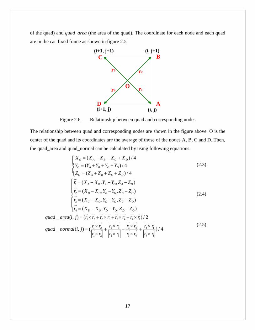
of the quad) and quad_area (the area of the quad). The coordinate for each node and each quad
are in the car-fixed frame as shown in figure 2.5.
(i+1, j)
(i+1, j+1) (i, j+1)
(i, j)
r1
r2r3
r4O
B
A
C
D
Figure 2.6. Relationship between quad and corresponding nodes
The relationship between quad and corresponding nodes are shown in the figure above. O is the
center of the quad and its coordinates are the average of those of the nodes A, B, C and D. Then,
the quad_area and quad_normal can be calculated by using following equations.
( ) / 4
( ) / 4
( ) / 4
O A B C D
O A B C D
O A B C D
X X X X X
Y Y Y Y Y
Z Z Z Z Z
(2.3)
1
2
3
4
( , , )
( , , )
( , , )
( , , )
A O A O A O
B O B O B O
C O C O C O
D O D O D O
r X X Y Y Z Z
r X X Y Y Z Z
r X X Y Y Z Z
r X X Y Y Z Z
(2.4)
1 2 2 3 3 4 4 1
2 3 3 41 2 4 1
1 2 2 3 3 4 4 1
_ ( , ) ( ) / 2
_ ( , ) ( ) / 4
quad area i j r r r r r r r r
r r r rr r r rquad normal i j
r r r r r r r r
(2.5)

18
Figure 2.7. Quad and normal direction plot for the upper surface
Figure 2.7 shows the directional normal of each quad. The cell_normal(i,j) matrix was
constructed to indicate the normal direction of each cell. The cell_normal(i,j) is different from
quad_normal(i,j) for the flat conventional cell, booster module and concentrator unit which is
always fixed to the sun.
2.2.5 Update the quad_marker matrix to implement a specified design
After following above steps, the design problem can be implemented in Matlab by updating the
quad_marker(i,j) to specify what type of solar array is used in the quad in a given design.
Different types of quad_marker(i,j) are given in the following table.
Table 3. Quad_marker table
Module quad_marker(i,j) cell_normal(i,j) Note
not_used 0 0 Not used area, will not generated energy
cnv_attach 1 quad_normal(i,j) Attached solar cells on upper surface
cnv_flat 0.5 [0 0 1]T Flat solar cells under the Acrylic cover
Cstr 2 facing to the sun Concentrator Unit, cell_normal(i,j) depends
on the sun, and will be addressed later
Bst 1.5 [0 0 1]T Booster module, only used in charging time

19
(node_marker(i,j)==2) &&
(node_marker(i+1,j)==2) &&
(node_marker(i,j+1)==2) &&
(node_marker(i+1,j+1)==2)
decide whether a quad is within the cstr unit area
quad_marker(i,j)=2
(5000 - L_tail - L_cstr <= X(i,j)) &&
(X(i,j) <= 5000-L_tail) &&
(abs(Y(i,j)) <= W_cstr/2)
decide whether a node is within the cstr unit area
node_marker(i,j)=2
(quad_x(i,j)>=1000+10 &&
quad_x(i,j)<=1000+L_bst-10 &&
abs(quad_y(i,j))<=300)
&& (quad_marker(i,j)==0)
decide whether a quad is used for the booster module
quad_marker(i,j)=1.5
Implement the Concentrator Unit Implement the Booster Module
area_cstr_cell = cstr_ratio * L_cstr * W_cstr / cos(theta_cstr);
area_bst_cell = L_bst * W_bst_cell;
N_flat = floor(max((6*10^6 - (area_attach_cnv + area_cstr_cell + area_bst_cell))/
step^2, 0));
temp_flat=N_flat; % temp counter
L_flat = max(5000 - L_tail - L_cstr - 2040, 0);
temp_x=floor((5000 - L_tail - L_cstr)/step);
if (L_flat > 0) % if there is space to place flat cnv cells
for j=1:temp_x % in fact, do not need temp_x, coz cstr have laready
overwrite corresponding portion
for i=1:N-1
if (quad_marker(i,j) == 0.5)
temp_flat=temp_flat-1;
if (temp_flat<=0) % no more flat cell to place
quad_marker(i,j) = 0;
end
end
end
end
end
Implement the 6m^2 constraintLoad the design variables
L_tail % lenth of cnv cells at tail
L_cstr % projected lenth of cstr unit in the H-plane
A_cstr % angle between cstr unit and H-plane
L_bst % length of the booster module
Figure 2.8. Flow chart of implementing a specified design
Figure 2.8 illustrates the rules of updating the quad_marker(i,j) in Matlab code. First, the values
of the design variables that are stored in the workspace are retrieved. Then, the quad is used for
the concentrator unit is determined. This process can be divided into two parts: (1) Checking
whether a node is in the concentrator unit; (2) Checking whether a quad is in the concentrator
unit. After that, implement the booster module, notice that the booster module use concentrator
cells. Finally, the 6 m2 total solar cell constraints are implemented and number of cells used in
the conventional solar cells under the Acrylic cover is decided. This order of updating the
quad_marker matrix will ensure that the energy production is best under the given design
variable value. The above process can also be called as the rules for implementing a specified
design. The updated quad_marker(i,j) matrix can be plotted to make sure the design is right
(refer to figure 2.3).
20
2.2.6 Energy production Calculation
Extraterrestrial Radiation
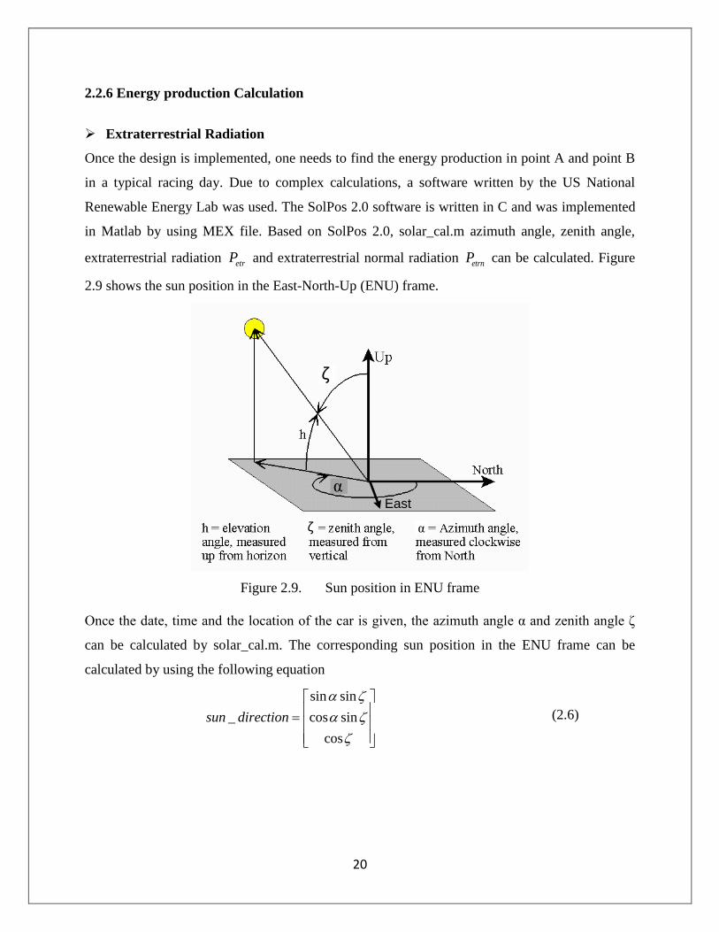
Once the design is implemented, one needs to find the energy production in point A and point B
in a typical racing day. Due to complex calculations, a software written by the US National
Renewable Energy Lab was used. The SolPos 2.0 software is written in C and was implemented
in Matlab by using MEX file. Based on SolPos 2.0, solar_cal.m azimuth angle, zenith angle,
extraterrestrial radiation etrP and extraterrestrial normal radiation etrnP can be calculated. Figure
2.9 shows the sun position in the East-North-Up (ENU) frame.
ζ
α
ζ α
East
Figure 2.9. Sun position in ENU frame
Once the date, time and the location of the car is given, the azimuth angle α and zenith angle ζ
can be calculated by solar_cal.m. The corresponding sun position in the ENU frame can be
calculated by using the following equation
sin sin
_ cos sin
cos
sun direction
(2.6)

21
Orientation of the car
We need to express the vector in car-fixed frame with respect to the ENU frame to calculate the
energy production. There are two cases: (1) the car heading towards north which corresponds to
the situation of the car in segment CD; (2) the car heading towards west which corresponds to
the situation of the car in segment DE.
x
yz
East
North
UpEast
North
Up
x
yz
(a) the car is heading to the north (b) the car is heading to the west
Figure 2.10. Relationship between the car-fixed frame and ENU frame
The figure above shows that the car is parallel to the horizontal plane (racing in a flat road). The
relationship between the two frames can be calculated by using the following equations.
ENU carV RV (2.7)
Where ENUV is the coordinate of the vector express in the ENU frame, carV is the coordinate of the
same vector expressed in the car-fixed frame. R is the corresponding rotation matrix. R=R1 for
situation (a) while R=R2 for situation (b). For faster computation, the components of the vector
are directly used instead of calling function dot.
1
0 1 0
1 0 0
0 0 1
R
, 2 3R I (2.8)
When the car is in charging station, it will be facing sun directly. It is relatively complex to
calculate the rotation matrix R. Notice that the effect is the same as if the sun is shining from the
top when we do not consider the atmospheric losses. Thus, we can use the following relation.
_ [0 0 1]Tsun direction (2.9)

22
Atmospheric Losses
The extraterrestrial normal radiation etrnP calculated by solar_cal.m is just radiation on the top of
the atmosphere. When the sun light transfers over the air, there will some losses. Ferman gave
several equations in his report, however, they simply assume that there will be about 6% losses
due to the atmosphere instead of adopting these complicated equations [2]
. However, this method
does not consider the length of the sun light path. Carroll gives the following empirical model [1]
0.3[cos( )]sq etrnP P (2.10)
where sqP is the power per square-meter produced by the solar cell when considering the energy
losses due to the transmission in atmosphere, etrnP is extraterrestrial normal radiation at the top of
atmosphere, ζ is the zenith angle of the sun. Thus, the power produced by a solar cell can be
calculated by using the following equation
0.3[cos( )] ( _ , _ )etrnP A P dot sun direction R cell normal (2.11)
where is the efficiency of the cell, A is the area of the cell, R is the rotation matrix in eq(8),
_cell normal is normal direction of the cell expressed in the car-fixed frame and _sun direction
is the position of the sun in ENU frame.
Energy calculation
The 2 points (A and B in figure 5) are used in solar_cal.m are as following:
%% point A: Omaham(mid pt of US route), heading to the NORTH lat = 41.257568; %Omaham(mid pt of US route) lon = -95.93718; yr = 2008; daynum = 195; %July-13-2008 zone = -6; % time zone sec = 00; % point B: Regina (mid pt of Canada route), heading to the WEST lat = 50.448015;%Regina (mid pt of Canada route) lon = -104.595179;
yr = 2008; daynum = 199; %July-17-2008 zone = -7; sec = 00;
The energy calculation is very complex and the flow chart is given in the figure below. Each case
corresponds to certain lines of Matlab code. Then for a specified design, design.m is executed

23
implement your design, then run solar_cal.m, energyA.m and energyB.m to get the result. Refer
to the matlab code for more information.
Charging time?
Racing time?
Iteration over time
quad_marker == 0.5?
quad_marker == 1?
quad_marker == 1.5?
quad_marker == 2?
Attached
conventional type
flat conventional
cells under cover
Booster module
Concentrator unit
Sun_direction = [0 0 1]’
Facing to the sun
Facing to the sun
Facing to the sun
Iteration over the
quad_marker
matrix
quad_marker == 0.5?
quad_marker == 1?
quad_marker == 2?
Attached
conventional type
flat conventional
cells under cover
Concentrator unit
Facing to the sun
Controlled by
motor
Iteration over the
quad_marker
matrix
Summation
Energy
production
Figure 2.11. Energy calculation flow chart
2.3 Meta-model Construction and Numerical Calculating
7 levels for each of the 4 design variables that were considered are given in the table below.
Variable Unit Upper
bound
Lower
bound Levels
L_tail mm 1240 1480 1240 1280 1320 1360 1400 1440 1480
L_cstr mm 1100 1400 1100 1160 1200 1260 1300 1360 1400
A_cstr deg 0 12 0 2 4 6 8 10 12
L_bst mm 0 1040 0 180 360 540 720 900 1040
Then, the energy production for each design is calculated. The results are plotted as following :

24
(a) L_tail = 1240 mm
(b) L_tail = 1280 mm
1100 1150 1200 1250 1300 1350 140005
10
0
200
400
600
800
1000
1200
Eng A (KWh), %L
tail =1240mm
Lcstr
(mm)A
cstr (deg)
Lbst (
mm
)
1100 1150 1200 1250 1300 1350 140005
10
0
200
400
600
800
1000
1200
Eng B (KWh), %L
tail =1240mm
Lcstr
(mm)A
cstr (deg)
Lbst (
mm
)
1100 1150 1200 1250 1300 1350 140005
10
0
200
400
600
800
1000
1200
Eng A (KWh), %L
tail =1280mm
Lcstr
(mm)A
cstr (deg)
Lbst (
mm
)
1100 1150 1200 1250 1300 1350 140005
10
0
200
400
600
800
1000
1200
Eng B (KWh), %L
tail =1280mm
Lcstr
(mm)A
cstr (deg)
Lbst (
mm
)

25
(c) L_tail = 1320 mm
(d) L_tail = 1360 mm
1100 1150 1200 1250 1300 1350 140005
10
0
200
400
600
800
1000
1200
Eng A (KWh), %L
tail =1320mm
Lcstr
(mm)A
cstr (deg)
Lbst (
mm
)
1100 1150 1200 1250 1300 1350 140005
10
0
200
400
600
800
1000
1200
Eng B (KWh), %L
tail =1320mm
Lcstr
(mm)A
cstr (deg)
Lbst (
mm
)
1100 1150 1200 1250 1300 1350 140005
10
0
200
400
600
800
1000
1200
Eng A (KWh), %L
tail =1360mm
Lcstr
(mm)A
cstr (deg)
Lbst (
mm
)
1100 1150 1200 1250 1300 1350 140005
10
0
200
400
600
800
1000
1200
Eng B (KWh), %L
tail =1360mm
Lcstr
(mm)A
cstr (deg)
Lbst (
mm
)
26
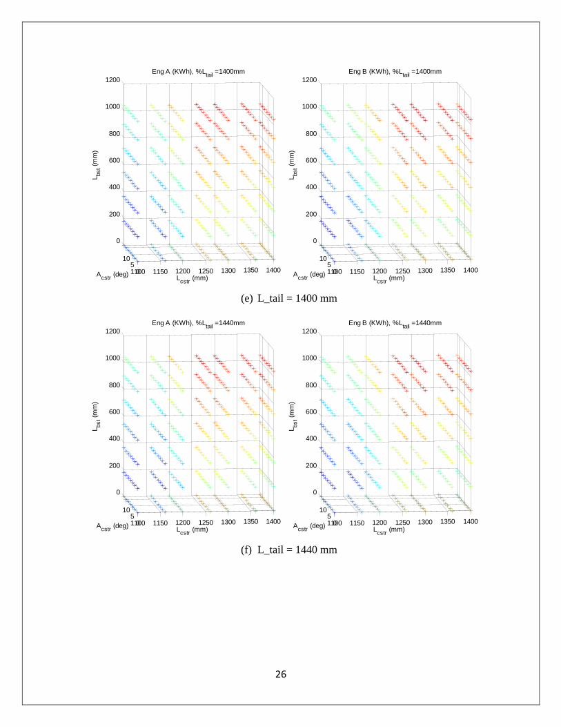
(e) L_tail = 1400 mm
(f) L_tail = 1440 mm
1100 1150 1200 1250 1300 1350 140005
10
0
200
400
600
800
1000
1200
Eng A (KWh), %L
tail =1400mm
Lcstr
(mm)A
cstr (deg)
Lbst (
mm
)
1100 1150 1200 1250 1300 1350 140005
10
0
200
400
600
800
1000
1200
Eng B (KWh), %L
tail =1400mm
Lcstr
(mm)A
cstr (deg)
Lbst (
mm
)
1100 1150 1200 1250 1300 1350 140005
10
0
200
400
600
800
1000
1200
Eng A (KWh), %L
tail =1440mm
Lcstr
(mm)A
cstr (deg)
Lbst (
mm
)
1100 1150 1200 1250 1300 1350 140005
10
0
200
400
600
800
1000
1200
Eng B (KWh), %L
tail =1440mm
Lcstr
(mm)A
cstr (deg)
Lbst (
mm
)
27
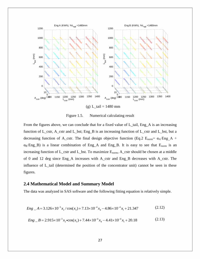
(g) L_tail = 1480 mm
Figure 1.5. Numerical calculating result
From the figures above, we can conclude that for a fixed value of L_tail, Eng_A is an increasing
function of L_cstr, A_cstr and L_bst; Eng_B is an increasing function of L_cstr and L_bst, but a
decreasing function of A_cstr. The final design objective function (Eq.2 Enorm= αA∙Eng_A +
αB∙Eng_B) is a linear combination of Eng_A and Eng_B. It is easy to see that Enorm is an
increasing function of L_cstr and L_bst. To maximize Enorm, A_cstr should be chosen at a middle
of 0 and 12 deg since Eng_A increases with A_cstr and Eng_B decreases with A_cstr. The
influence of L_tail (determined the position of the concentrator unit) cannot be seen in these
figures.
2.4 Mathematical Model and Summary Model
The data was analyzed in SAS software and the following fitting equation is relatively simple.
3 4 4
2 3 4 1_ 3.126 10 / cos( ) 7.13 10 4.86 10 21.347Eng A x x x x (2.12)
3 4 4
2 3 4 1_ 2.915 10 cos( ) 7.44 10 4.41 10 20.18Eng B x x x x (2.13)
1100 1150 1200 1250 1300 1350 140005
10
0
200
400
600
800
1000
1200
Eng A (KWh), %L
tail =1480mm
Lcstr
(mm)A
cstr (deg)
Lbst (
mm
)
1100 1150 1200 1250 1300 1350 140005
10
0
200
400
600
800
1000
1200
Eng B (KWh), %L
tail =1480mm
Lcstr
(mm)A
cstr (deg)
Lbst (
mm
)
28
Where
1
2
3
4
_
_
_
_
x L tail
x L cstr
x A cstr
x L bst
R-square(A) = 0.8365, F-value(A)=4087.85; R-square(B)=0.8425, F-value(B)=4273.13. These
values indicates that the model is very good. We can further modify the model as following
2 3 4 1
2 3 4 1
_ 3.126 / cos( ) 0.713 0.486 21.347
_ 2.915 cos( ) 0.744 0.441 20.18
Eng A x x x x
Eng B x x x x
where
3
1
3
2
3
3
4
10 _
10 _
_
10 _
x L tail
x L cstr
x A cstr
x L bst
Recall Eq(2), where we have Enorm= αA∙Eng_A + αB∙Eng_B, where αA = 0.6 and αB = 0.4. The
objective function can be stated as below.
1 2 3 4
2 3 3 4 1, , ,
(1.8756/ cos 1.166cos ) 0.7254 0.468 20.88max normx x x x
E x x x x x (2.14)
The mathematical model (which is also the summary model) is given as following
1 2 3 4
2 3 3 4 1, , ,
1 1
2 1
3 2
4 2
5 3
6 3
7 4
8 4
(1.8756 / cos 1.166cos ) 0.7254 0.468 20.88
. .
:1.24 0
: 1.48 0
:1.1 0
: 1.4 0
: 0
: 12 0
: 0
: 1.04 0
minx x x x
f x x x x x
s t
g x
g x
g x
g x
g x
g x
g x
g x
(2.15)
29
2.5 Model Analysis
The mathematical model of this subsystem is simple. It can be easily seen from Eq(15) that the
objective function f is an increasing function of 1x , and decreasing function of 2x and 4x .
Therefore, by MP1,
1 1
2 2
4 4
1.24
1.4
1.04
lb
ub
ub
x x
x x
x x
The design problem can be further simplified as:
3
3 3
5 3
6 3
(2.656 / cos 1.6324cos ) 21.0544
. .
: 0
: 12 0
minx
f x x
s t
g x
g x
(2.16)
Let 3cost x , then the design problem can be transferred into
1
2
' (2.656 / 1.6324 ) 21.0544
. .
: cos(12 ) 0.9781 0
: 1 0
mint
f t t
s t
g t t
g t
(2.17)
The first order derivative of f‟ with respect to t is 21.6432 2.656 / t , which is positive in the
feasible set [0.9781,1]t , which indicates that f‟ is an increasing function of t. Therefore, t
should selected as the lower bound, which is 0.9781. For
1 1 2 2 3 2 4 41.24, 1.4, 12, 1.04lb ub ub ubx x x x x x x x
Enorm has the max value, and max(Enorm)=25.3665..
The original Enorm before curve fitting, calculated by Matlab code for this design variable is
25.2902, which is nearly the same as the fitting result.
2.6 Summary and Discussion
Most solar cars just have the conventional attached solar cells. Continuum has4 types of solar
cell sub-module: (1) conventional attached solar cells; (2) conventional solar cells under the
Acrylic cover; (3) booster module; (4) concentrator system, all of which makes the modeling
work complex. The problem dealt as following and a mathematical model was developed.

30
(1) The upper-surface was divided into 20000 small quads. The quad_marker matrix was
formed to identify which type of solar array the small quad will be use. Two properties
quad_area and quad_normal associated with quad_marker matrix are used. Therefore,
one can manipulate the data of the solar car directly through Matlab instead of
Solidworks. This was the foundation of the solar array subsystem optimization.
(2) Four design variables L_tail, L_cstr, A_cstr and L_bst were identified and implement for
the design process in Matlab. The design process was transformed by updating the
quad_marker matrix according the value of design variables and constraints.
(3) The energy production was calculated considering 7 scenarios for a point.
(4) The results were plotted in Matlab and the data was analyzed in SAS.A simple
mathematical model was formed using the SAS software. The R-square value and the F-
value is very good in the sense of statistics.
The model was also analyzed using monotonicity principle, the model agrees well to the
original data calculated by Matlab. The optimal design for the subsystem was derived.
The reason for the strong monotonicity of the design variables in the design objective is because
of the unused area on the upper surface .Although the direction normal is very complex for the
whole system. For example, the unused result in the code was traced and it was found that the
unused area is a decreasing function of L_cstr, A_cstr and L_bst, and is an increasing function of
L_tail. The energy productions at these two points have the opposite monotocity as the unused
area except Eng_B with respect to A_cstr. The reason might be the solar car is heading to the
west at point B.
It should be pointed out that due to the physical difficulties for implementation; the space left for
the solar array subsystem optimization is relatively small. Further one can focus on serial and
parallel drives in order to generate certain voltage and current to drive the motor link of these
solar cells.

31
Subsystem 2: Long Term Strategy Optimization –Chiao-Ting Li
Solar car long term race strategy aims at optimizing cruising speeds in order to finish the race as
fast as possible while still taking into account the race rules, battery and motor hardware
realities. The race starts at Dallas and ends at Calgary; totally 3578 km long with 4 stage stops
and 6 check points on the way (see Figure 3.1. and Table 3.1. ). According to the rule, solar cars
are asked to pull in for 30 minutes at the stage stops and check points. The solar array is allowed
to tilt toward the sun in these 30-minute charging to have better charging. Solar car can resume
and keep running after check point pull-in, but stage stops are mandatory camp sites. Solar car
teams are asked to camp there overnight. At the stage stop camping, solar car battery will be
impounded after the 30-minute pull-in charging and released at 6 PM to allow the evening sunset
charging. Later in this section the stage stops and check points will be called as pull-in events.
The distance between pull-in events ranges 200 ~ 400 km, and a solar car is expected to pass one
or two of them in every running day. The charging hour can be from sunrise to sunset, but no
early than 6:30AM and no later than 8:30PM. A regular day running hour is 8 AM to 6 PM,
while a stage start day running hour is 9 AM to 6 PM. The purpose of stage stops and check
points is to provide opportunity for media and public to see the teams in action, and also create a
chance to let the slower teams to catch up and make the race more competitive. The winner is the
one has the shortest running time.
Figure 3.1. NASC race route

32
Table 3.1. Preliminary schedule of 08‟ NASC by town
Event City Dist. (km) Nomenclature
Start Dallas, Texas, USA -
Checkpoint McAlester, OK, USA 274 dist1
Stage Stop Neosho, MO, USA 288 dist2
Checkpoint Topeka, KS, USA 370 dist3
Checkpoint Omaha, Nebraska, USA 267 dist4
Stage Stop Sioux Falls, South Dakota, USA 291 dista
Checkpoint Fargo, North Dakota, USA 390 dist7
Stage Stop Winnipeg, Manitoba, CANADA 355 dist8
Checkpoint Brandon, Manitoba, CANADA 214 dist9
Checkpoint Regina, Saskatchewan, CANADA 362 dist10
Stage Stop Medicine Hat, Alberta, CANADA 472 distb
Finish Calgary, Alberta, CANADA 293 dist13
3.1 Problem Statement
The solar array power production varies because solar incident angle changes with time. The
power production is characterized as a concave function of time, which has maximum at noon,
and increases in the morning and decreases in the afternoon. This characteristic makes battery
play an important role in the long term strategy: to use it as energy buffer and maintain solar car
at constant speed throughout the race.
A constant speed running has been mathematically proved to be the optimal strategy for ideal flat
route [3].Constant power or constant torque are then brought out as practical alternatives. Some
control approaches are also seen in the literature [7,9]. However, they don‟t really take into
account battery remnant balance or the 30-minute stops in to consideration. The secondary goal
(besides minimizing running time) of this optimization is to have the program iterate out the
optimal battery remnant at end of running every day instead of having the strategist manually
specify it by trail-and-error.
The stage stops and check points make the long term strategy problem somehow discontinuous
and complex. A previous modeling idea was to partition the race route into several segments, and
define two small optimization problems according to different running scenarios. However, since
the ultimate race goal is to minimize total running time, the same partition idea is used, but the
partitioned segments are connected together and the race route is modeled as a whole instead of
several distributed segments, and the optimization problem is to find the thirteen speed variables

33
at one go to have shortest racing time. The route partition is described in section 3.3.1.
3.2 Nomenclature
Table 3.1. Nomenclature for long term strategy subsystem
Name Unit Description Classification
m kg Vehicle mass Parameter
g m/s2 9.81, gravitational constant Constant
Crr - Coefficient of rolling resistance Parameter
Cd - Coefficient of aerodynamic drag Parameter
Cl - Coefficient of lift force Parameter
A m2 Frontal area Parameter
ρ kg/m3 1.23, air density Constant
vi m/s Vehicle speed of the i-th segment Variable
vL m/s US highway speed limit Constant
η - Powertrain efficiency Parameter
E Ws Energy Interim term
Pv W Solar car power consumption Interim term
Parray W Solar array power production Interim term
P’array W Inclined solar array power production Interim term
Pmax W Solar array maximum power production Parameter
Pmisc W Solar car miscellaneous power consumption Parameter
z degree Zenith angle Interim term
BRini Ws Initial battery remnant Parameter
BRi Ws Battery remnant of the beginning or end of a day Interim term
BRfull Ws Battery capacity Parameter
ti min Time used in the i-th running segment Interim term
tstr,1 min 480, starting hour of day 1 (i.e 8AM) Constant
tstr,2 min 540, starting hour of day 2 (i.e 9AM) Constant
tstr,3 min 480, starting hour of day 3 Constant
tstr,4 min 540, starting hour of day 4 Constant
tstr,5 min 540, starting hour of day 5 Constant
tstr,6 min 480, starting hour of day 6 Constant
tstr,7 min 540, starting hour of day 7 Constant
tavail,1 min 600, available running hours of day 1 (i.e. 10 hours) Constant
tavail,2 min 540, available running hours of day 2 (i.e. 9 hours) Constant
tavail,3 min 600, available running hours of day 3 Constant
tavail,4 min 540, available running hours of day 4 Constant
tavail,5 min 540, available running hours of day 5 Constant
tavail,6 min 600, available running hours of day 6 Constant
tavail,7 min 540, available running hours of day 7 Constant
dist5 km Distance of the 5-th running segment Interim
dist6 km Distance of the 6-th running segment Interim
dist11 km Distance of the 11-th running segment Interim
34
dist12 km Distance of the 12-th running segment Interim
R m Tire radius, 0.254 Parameter
T Nm Vehicle load Interim term
3.3 Mathematical Model
A true model was built to understand the behavior of the system, especially the battery remnant
drop and events of over-discharge/overcharge hazards. Then a great deal of curve fits and surface
fits are utilized to build a metamodel. Comparison of the true model and the metamodel are done
for validation.
3.3.1 Assumptions
To simplify the long term strategy and focus on balance of solar power production and vehicle
power consumption in a long time scale, route details and other disturbances are not included in
the model but left to the short term strategy. The following assumptions are been made:
No grade route.
All sunny weather.
No winds.
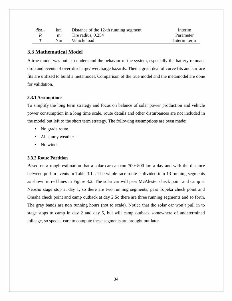
3.3.2 Route Partition
Based on a rough estimation that a solar car can run 700~800 km a day and with the distance
between pull-in events in Table 3.1. . The whole race route is divided into 13 running segments
as shown in red lines in Figure 3.2. The solar car will pass McAlester check point and camp at
Neosho stage stop at day 1, so there are two running segments; pass Topeka check point and
Omaha check point and camp outback at day 2.So there are three running segments and so forth.
The gray bands are non running hours (not to scale). Notice that the solar car won‟t pull in to
stage stops to camp in day 2 and day 5, but will camp outback somewhere of undetermined
mileage, so special care to compute these segments are brought out later.

35
Far
go
Ba
tte
ry r
em
na
nt
Time
Day 1 Day 2 Day 3 Day 4 Day 5 Day 6 Day 7
McA
lest
er
Topek
a
Om
aha
Win
nip
eg
Bra
ndon
Reg
ina
Cal
gar
y
Outb
ack
Outb
ack
v1
v2
v3
v4
v5
v6
v7
v8
v9
v10
v11
v12 v13
Neo
sho
BR1
BR2
BR3BR7
BR4
Sio
ux F
alls
BR6 BR8
BR9
BR10
BR11
Med
icin
e H
atBR5
BR12
BR13
Figure 3.2. Route partition
3.3.3 True Model
The true model consists of two parts: vehicle model which computes power consumption, and
array model which computes power production.
3.3.3.1 Vehicle Model
Firstly, aero drag force and lift force are calculated:
21
2aero dF C Av (3.1)
21
2lift lF C Av (3.2)
Then rolling resistance force can be found using following relation:
roll rr liftF C mg F (3.3)
The vehicle power consumption is due to aero drag, rolling resistance and miscellaneous power.
The expression is given below.
2 2
1
1 1 1
2 2
v aero roll misc
d rr l mv isc
P F F v P
C Av C mg C AvP P
(3.4)
The power train efficiency η is calculated by an experimental fit formula:
0.1765T
(3.5)
where ω is the motor revolution speed, T is the vehicle load:

36
v
R (3.6)
aero rollT F F v (3.7)
Figure 3.3. gives the vehicle power as an increasing function of speed.
Figure 3.3. Vehicle power consumption
Although the lift force and powertrain efficiency make the vehicle power consumption equation
not explicitly cubic polynomial, the overall vehicle power curve are still quite close to cubic
function.
3.3.3.2 Array Model
A simplified array power production is used here rather than the detailed model in array
optimization subsystem. The solar array power production is approximated as maximum array
output times solar incident angle [1]:
1.3
cosarray maxP = P z (3.8)
where z is the zenith angle (see Figure 3.4. ), the 1.3 order is experimental fit coefficient for
atmosphere diffusion correction. SolPos 2.0, an existing piece of C code written by the US
National Renewable Energy Lab, is used to calculate the zenith angle. SolPos 2.0 does not use
the circular orbit assumption and instead uses the more exact elliptical orbit of the earth around

37
the sun that it is able to gain an accuracy up to ± 0.0003 degrees[2]. A MALAB MEX wrapper is
written to interface the SolPos C code and MATLAB.
Inclined array power production is approximated by another experimental fit equation:
0.3
cosarray maxP = P z (3.9)
Figure 3.4. Solar incident angle
After two programs for power consumption and production are created, the true model computes
the accumulated net energy in a for loop by 1 minute time discretization with initial speed
assumptions and updates mileage and battery remnants for every minute. Figure 3.5. shows the
SOC history of day 1 with the initial speed assumption as 28 m/s for the first two running
segments. Notice that although Ws unit is used for battery remnant in calculation, unit
conversion to Wh is made when plotting throughout the long term strategy section to give the
reader a more human sensible scale about the remnant. It indicates that the solar car will pull in
to the first check point at 10:47AM, which corresponds to the first SOC bounce in Figure 3.5.
and pull in to the first stage stop at 2:03 PM. The dash line indicates that the battery is
impounded after the 30-minute charging at the stage stop.

38
Figure 3.5. Day 1 SOC history
The true model was built to only simulate single day running to study the system behavior, and
one needs to manually input the speed for every running segments for every simulation and there
is no optimization been imposed onto the true model.
MATLAB is slow in computing multiple cascade loops hence a metamodel was built to lump the
array power computation.
3.3.4 Metamodel
Four lumped curves/surfaces are generated and put together as the metamodel to ease the array
power computation.
3.3.4.1 Sunrise/Sunset Charging Curve Fits
Using 1-minute time discretization, the sunrise power throughout the race route was calculated in
advance and accumulated as total energy income. So every data point holds energy, not just
power. By visual examination, a quadratic fit was chosen to fit the curve. The true model data is
shown is Figure 3.6. . Because of the time zone crossing, the curve shape has a twist in the
middle. The resulting curve fit equation is as:
2 60.2496 641 7.291 10SRE x x x (3.10)

39
where x is the mileage in km, and ESR is the sunrise charging energy in Ws. The fit confidence,
R-square is 0.9566, which indicates quadratic function is adequate for our purpose here.
Figure 3.6. Sunrise charging energy and its quadratic curve fit
Similar approach is implemented for sunset charging curve, but instead a linear fit was chosen
this time. The true model data is plotted in Figure 3.7. and the resulting line equation is:
2 62188 4.584 10SSE x x (3.11)
where x is again the mileage in km, and ESS is the sunset charging energy in Ws. The fit
confidence, R-square is 0.989, which indicates linear function is enough to do this fit.
Figure 3.7. Sunset charging and its linear curve fit
40
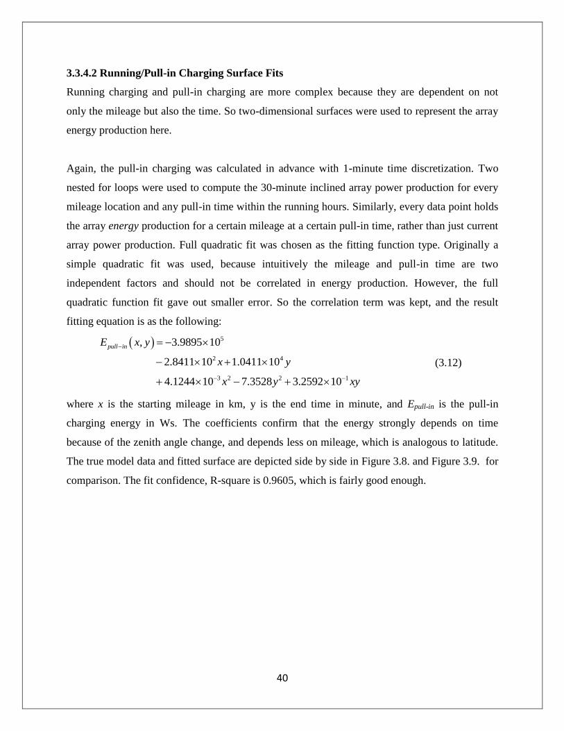
3.3.4.2 Running/Pull-in Charging Surface Fits
Running charging and pull-in charging are more complex because they are dependent on not
only the mileage but also the time. So two-dimensional surfaces were used to represent the array
energy production here.
Again, the pull-in charging was calculated in advance with 1-minute time discretization. Two
nested for loops were used to compute the 30-minute inclined array power production for every
mileage location and any pull-in time within the running hours. Similarly, every data point holds
the array energy production for a certain mileage at a certain pull-in time, rather than just current
array power production. Full quadratic fit was chosen as the fitting function type. Originally a
simple quadratic fit was used, because intuitively the mileage and pull-in time are two
independent factors and should not be correlated in energy production. However, the full
quadratic function fit gave out smaller error. So the correlation term was kept, and the result
fitting equation is as the following:
5
2 4
3 2 2 1
, 3.9895 10
2.8411 10 1.0411 10
4.1244 10 7.3528 3.2592 1
,
, 0
pull in
Pull i
pull in
n
E x y
E
E x y
x y
x yy xyx
(3.12)
where x is the starting mileage in km, y is the end time in minute, and Epull-in is the pull-in
charging energy in Ws. The coefficients confirm that the energy strongly depends on time
because of the zenith angle change, and depends less on mileage, which is analogous to latitude.
The true model data and fitted surface are depicted side by side in Figure 3.8. and Figure 3.9. for
comparison. The fit confidence, R-square is 0.9605, which is fairly good enough.

41
Figure 3.8. Pull-in charging from true model
Figure 3.9. Pull-in charging from surface fit
The same surface equation generation procedure is repeated for running charging, but the fitting
function type selection is different. A first glance of the true data (see Figure 3.10. ) shows that
the energy merely depends on the mileage, so a plane function was first tried, but the error
statistics was large.This led to use higher order surface functions. The second try was a full
quadratic fit. Although the R-square was nice, but there were numbers below zero, which might
cause troubles in later stage, so full cubic equation was chosen in the end, and the resulting
equation is as the following.
7
4 5
2 2 2 1
5 3 1 3 4 2 2 2
, 4.2325 10
1.2776 10 3.0275 10
1.1595 5.6088 10 2.8114 10
8.6998 10 2.5457 10 5.3458 10 1.4422 1
,
,
0,
run
run
Run
Run
E x y
xE x y
E x y
E
y
x y xy
x y y xyx y x
(3.13)
where x is the starting mileage in km, y is the end time in minute, and Erun is the running
charging energy in Ws. The coefficients of higher order terms of x are very small indicating it is
over fit to use such high order polynomial to do the fit. As stated above such high order function
is just for resolving the less-than-zero problem. The cubic fit confidence, R-square, is 0.9994.
The data from true model is shown in Figure 3.10. and the comparison of quadratic and cubic
fits is shown in Figure 3.11. and Figure 3.12. .
0
2000
4000
8 10 12 14 16 18
2
2.2
2.4
2.6
2.8
3
3.2
3.4
x 106
Dist [km]Time [hr]
Energ
y [
W-s
]
0
2000
4000
8 10 12 14 16 18
2.2
2.4
2.6
2.8
3
3.2
3.4
x 106
Dist [km]Time [hr]
Energ
y [
W-s
]

42
Figure 3.10. Running charge from true model
Figure 3.11. Running charging and
quadratic surface fit
Figure 3.12. Running charging
and cubic surface fit
3.3.4.3 Battery Remnant
The true model study shows that the interim SOC can never be higher than that at start of the
day, and never be less than that at end of the day. Hence in the metamodel, the battery remnant is
simplified as computing SOC when start out and camp, which are the BR1 to BR13 in Figure 3.2. .
01000
20003000
4000
810121416180
1
2
3
4
5
x 107
Dist [km]Time [hr]
Energ
y [
W-s
]
01000
20003000
4000
81012141618-1
0
1
2
3
4
5
6
x 107
Ture
Fit
Dist [km]Time [hr]
Energ
y [
W-s
]
01000
20003000
4000
81012141618-1
0
1
2
3
4
5
6
x 107
Dist [km]
TureFitting
Running charge, cubic fit
Time [hr]
Energ
y [
W-s
]

43
1 2
2
1 0 ,1 1 2 1 ,1 1 1 2
1
, 30 , run i str pull in str v v
i
BR BR E dist t t t E dist t t P t P t
(3.14)
2 2 2
2 1 ,1 1 2
1 1 1
, 30pull in i str SR i SS i
i i i
BR BR E dist t t t E dist E dist
(3.15)
3 4 5
5
3 2 ,2 ,2
1
3 4
,2 3 ,2 3 4
1
3
1
3 4 5
3
,
, , 30
run i str avail
i
pull in i str pull in i str
i i
v v v
BR BR E dist t t
E dist t t E dist t t t
P t P t P t
BR
BR
(3.16)
5 5
4 3
1 1
SR i SS i
i i
BR BR E dist E dist
(3.17)
6
6
5 4 ,3 6 6
1
, run i str v
i
BR BR E dist t t P t
(3.18)
6 6 6
6 5 ,3 6
1 1 1
, pull in i str SR i SS i
i i i
BR BR E dist t t E dist E dist
(3.19)
7 8
8 7
7 6 ,4 7 8 ,4 7
1 1
7 87
, 30 , run i str pull in i str
i i
v v
BR BR E dist t t t E dist t t
P tBR P t
(3.20)
8 8 8
8 7 ,4 7 8
1 1 1
, 30pull in i str SR i SS i
i i i
BR BR E dist t t t E dist E dist
(3.21)
9 10 11
11
9 8 ,5 ,5
1
9 10
,5 9 ,5 9 10
1 1
9 10 11
9
9
,
, , 30
run i str avail
i
pull in i str pull in i str
i i
v v v
BR BR E dist t t
E dist t t E dist t t t
P t P t P
BR
tBR
(3.22)
11 11
10 9
1 1
SR i SS i
i i
BR BR E dist E dist
(3.23)
12
12
11 10 ,6 12 12
1
, run i str v
i
BR BR E dist t t P t
(3.24)

44
12 12
12 11
1 1
SR i SS i
i i
BR BR E dist E dist
(3.25)
13
13
13 12 ,7 13 13
1
, run i str v
i
BR BR E dist t t P t
(3.26)
3.3.4.4 Metamodel Validation
So now one can take a set of speed initial guess and compute the segment time by the equations
in section 3.3.5 and plug in the segment time and the mileage into the 4 lumped energy
equations. Then the battery remnant can be found in less than one second compare to couple of
seconds or so in the true model simulation. Figure 3.13. shows the SOC trajectory of day 2 with
an arbitrary set of speed initial guess for every segment. The SOC points are connected simply
by straight line for better illustration, but one should keep in mind that the metamodel actually
computes the battery remnant for beginning and end of the day only.
Figure 3.13. Day 2 simulation by the metamodel
A comparison between the true model and the metamodel has been made to validate if the
metamodel functions reasonably. Figure 3.14. shows the day 1 SOC true model simulation and
metamodel results with all speed initial guess as 28 m/s. the results are quite consistent. The true
model predicted BR1 (SOC at around 2 PM in the figure) to be 1277592 Ws, while the
metamodel predicted BR1 as 512953 Ws. The absolute difference seems large, but actually it

45
corresponds to only 5% capacity of the 5kWh (18000000 Ws) battery bank, which is acceptable
for our purpose to solve the long term strategy as a design problem.
Figure 3.14. Comparison of the day 1 SOC simulation results
of true model and metamodel
3.3.5 Objective Function
Now we have a suitable route partition and metamodel to describe the solar car running. The
next is to form an optimization problem to find optimal speed for every running segment.
The objective function of long term strategy is the total running time:
1 2 3 4 5 6 7 8 9 10 11 12 13f t t t t t t t t t t t t t (3.27)
where
8 9 10 11 12 13 14 15 16 17 180
500
1000
1500
2000
2500
3000
3500
4000
4500
5000
Time [hr]
Batt
ery
SO
C [
Wh]
true mdl
metamdl

46
31 2 41 2 3 4
1 2 3 4
5 ,2 3 4
5 5 5
6 5
6 7 8 9 106 7 8 9 10
6 7 8 9 10
11 ,5 9 10
11 11
, , ,
30 30
, , , ,
30 30
avail
a
avail
distdist dist distt t t t
v v v v
t t t t
dist v t
dist dist dist
dist dist dist dist distt t t t t
v v v v v
t t t t
dist v t
11
12 11
131212 13
12 13
,
bdist dist dist
distdistt t
v v
(3.28)
Notice that t5 and t11 are different than others that they are not the simple distance dividing by
speed because as mentioned before that the camp mileage of day 2 and day 5 are undetermined,
so the corresponding running segment time is computed by subtracting the available running
hours from the used time of previous running segments of the current day.
3.3.6 Design Variables and Parameters
The design variables are the thirteen speeds v1 ~ v13. There is upper bound from the US highway
speed limit to be 65 mph (~29 m/s). The maximum speed of Continuum solar car is more than 80
mph, which is higher than the highway speed limit. So we don‟t use that as the upper bound for
our design variable and the speeds need to be positive.
0 , 1...13i Lv v i (3.29)
As listed in Table 3.1. , design parameters are vehicle mass, m, array max power Pmax, battery
capacity BRfull, battery initial BRini, and couple of vehicle specification values, including Crr, Cd,
Cl, A, R, Pmisc. The first four (m, Pmax, BRfull, BRini) will be examined during the parametric study
in later section 3.7 as the preparation for system integration.
3.3.7 Constraints
There are inequality constrains on battery remnants, and segment times.
The battery should not overcharge or over-discharge, so the corresponding constraints are:
0 , 1...13i fullBR BR i (3.30)

47
The inequality constraints on segment times make sure that the solar car really runs along the
defined route partition, and also help to fulfill the time reduction when pull-in to stage stops.
1 2 ,1avilt t ct
6 ,3avilt t
7 8 ,4avilt t t
12 ,6avilt t
13 ,7availt t
(3.31)
Furthermore, there are two equality constraints imposed amount t3, t4, t5 and t9, t10, t11 when
computing t5 and t11 in section 3.3.4.3. They are again summarized here:
3 4 5 ,2availt t t t
9 10 11 ,5availt t t t (3.32)
3.4 Summary Model
The long term strategy running time minimization optimization problem is summarized in
negative null form as:

48
1 2 3 4 5 6 7 8 9 10 11 12 130 , 1...13
mini Lv v i
f t t t t t t t t t t t t t
1 1
2 1
3 2
4 2
5 3
6 3
7 4
8 4
9 5
10 5
11 6
12 6
13 7
14 7
15 8
16 8
s.t.
0
0
0
0
0
0
0
0
0
0
0
0
0
0
0
full
full
full
full
full
full
full
ful
g BR
g BR BR
g BR
g BR BR
g BR
g BR BR
g BR
g BR BR
g BR
g BR BR
g BR
g BR BR
g BR
g BR BR
g BR
g BR BR
17 9
18 9
19 10
20 10
21 11
22 11
23 12
24 12
25 13
26 13
27 1 2 ,1
28 6 ,3
29 7 8 ,4
3
0
0
0
0
0
0
0
0
0
0
0
0
0
0
l
full
full
full
full
full
avail
avail
avail
g BR
g BR BR
g BR
g BR BR
g BR
g BR BR
g BR
g BR BR
g BR
g BR BR
g t t t
g t t
g t t t
g
0 12 ,6
31 13 ,7
0
0
avail
avail
t t
g t t
(3.33)

49
1 3 4 5 ,2
2 9 10 11 ,5
0
0
avail
avail
h t t t t
h t t t t
(3.34) contd.
3.5 Model Analysis
3.5.1 Equality Constraints
The two equality constraints, h1 and h2, are plugged into the objective function .The objective
function becomes:
1 2 ,2 6 7 8 ,5 12 13avail availf t t t t t t t t t (3.35)
In this way, the design variables, v3, v4, v5 and v9, v10, v11 are not seen in the objective function
any more, but they still show in the constraints and have effects on the optimization problem.
3.5.2 Constraint Redundancy
From intuition and the true model simulation, one can simply see that the battery remnant at
beginning of a day (BR2, BR4, BR6, BR8, BR10, BR12) tend to have overcharge because of the
sunset charging lest evening and sunrise charging in the early morning. So the lower bound
constraints are inactive for these terms (g3, g7, g11, g15, g19, g23). On the other hand, the battery
remnant at end of a day (BR1, BR3, BR5, BR7, BR9, BR11, BR13) tend to have over discharge, and
the upper bound constraints are inactive for these terms (g2, g6, g10, g14, g18, g22, g26).
3.5.3 Feasible Set
The objective contour of only day 1 running times (i.e. 1 2f t t only) is depicted in Figure
3.15. to further study the feasible set. The x1 in horizontal-axis and x2 in vertical-axis are the two
design variable v1 and v2 in day 1. The related variable bounds and constraints are plotted by
black bold lines. It was found that the feasible set is quite small, which is due to the somehow
too optimistic array model. The array model will be examined further during the parametric
study in section 3.7. Also it can be seen that the segment time constraint, g27, is far loose than the
battery remnant constraints g4. Although couldn‟t prove mathematically, it is quite sure that the
battery remnant upper bound constraints in the stage stop days will dominate the segment time
constraints (g4 dominates g27, g12 dominate g28, g16 dominates g29, and g24 dominate g30). So even
though the segment time constraints, g27 ~ g30, have the same monotonicity as the objective
function does, they can be ruled out.

50
300
350
350
40
0
400
400
45
0
450
450
50
0
500
500
55
0
550
550
550
60
0
600
600
600
65
0
650
650
650
70
0
70
0
700
700700
75
0
75
0
750
750750
80
0
80
0
800
800800
85
085
0
850
850850
90
090
0
900
900900950
950
95
0
95
0
1000
1000
10
00
1050
10
50
1100
11
00
1150
12001250
13001350
x1
x2
Objective contoure
10 15 20 25 30
10
15
20
25
30
g1
g4
Feasible set
g27
Figure 3.15. Feasible set of one day running
Feasible set with more design variables are not depicted because of the dimension is more than
three and cannot be represented spatially.
3.5.4 Monotonicity
According to the simplified objective function equation in section 3.5.1, it is apparent that the
objective is monotonically increasing with respect to t1, t2, t6, t7, t8, t12, and t13, so is
monotonically decreasing with respect to design variables v1, v2, v6, v7, v8, v12, and v13. However,
because of the accumulated battery remnant constraints, it is almost impossible to derive explicit
equation expression design variables and draw conclusions about monotonicity of the
constraints.
3.5.5 Well-Boundedness
A feasible solution was found by trail-and-error, which confirms that the feasible set is non
empty. This solution is then used as initial guess in the optimization later. Also the design
variables are bounded from top and bottom, so the problem will at least have bounded optima.

51
3.5.6 Model Simplification
After the model analysis, the model is simplified and summarized as the following
1 2 ,2 6 7 8 ,5 12 130 , ...13
mini L
avail availv v i
f t t t t t t t t t
1 1
2 2
3 3
4 4
5 5
6 6
7 7
8 8
9 9
10 10
11 11
12 12
13 13
s.t.
0
0
0
0
0
0
0
0
0
0
0
0
0
full
full
full
full
full
full
g BR
g BR BR
g BR
g BR BR
g BR
g BR BR
g BR
g BR BR
g BR
g BR BR
g BR
g BR BR
g BR
(3.36)
3.6 Numerical Results
The optimization function fmincon in MATLAB was used to solve the solar car long term
strategy speed optimization problem. The constrained solution was found; unbounded design
variables and released constraints solutions were also studied.
3.6.1 Unbounded variable
The unbounded variable case was probed to understand if the problem is well-constrained
without design variable bounds. The answer turned out to be yes, and constraints g2, g6, g7, g10,
g12, g13 are active. The SOC history of whole race route and speed minimizers is plotted in
Figure 3.16. , and the total running time (optimal function value) is 2330.22 minute.
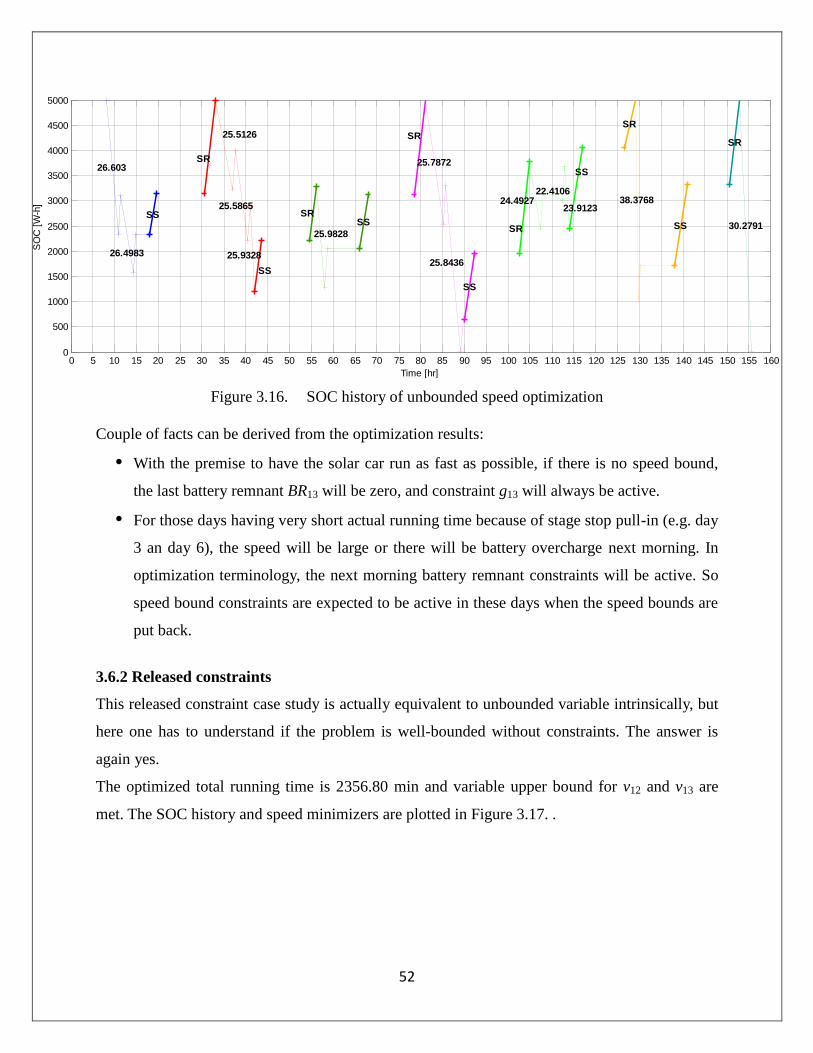
52
Figure 3.16. SOC history of unbounded speed optimization
Couple of facts can be derived from the optimization results:
With the premise to have the solar car run as fast as possible, if there is no speed bound,
the last battery remnant BR13 will be zero, and constraint g13 will always be active.
For those days having very short actual running time because of stage stop pull-in (e.g. day
3 an day 6), the speed will be large or there will be battery overcharge next morning. In
optimization terminology, the next morning battery remnant constraints will be active. So
speed bound constraints are expected to be active in these days when the speed bounds are
put back.
3.6.2 Released constraints
This released constraint case study is actually equivalent to unbounded variable intrinsically, but
here one has to understand if the problem is well-bounded without constraints. The answer is
again yes.
The optimized total running time is 2356.80 min and variable upper bound for v12 and v13 are
met. The SOC history and speed minimizers are plotted in Figure 3.17. .
0 5 10 15 20 25 30 35 40 45 50 55 60 65 70 75 80 85 90 95 100 105 110 115 120 125 130 135 140 145 150 155 1600
500
1000
1500
2000
2500
3000
3500
4000
4500
5000
Time [hr]
SO
C [
W-h
]
Whole soc history estimation
26.603
26.4983
SS
SR
25.5126
25.5865
25.9328
SS
SR
25.9828
SS
SR
25.7872
25.8436
SS
SR
24.492722.4106
23.9123
SS
SR
38.3768
SS
SR
30.2791
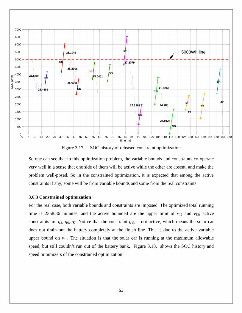
53
Figure 3.17. SOC history of released constraint optimization
So one can see that in this optimization problem, the variable bounds and constraints co-operate
very well in a sense that one side of them will be active while the other are absent, and make the
problem well-posed. So in the constrained optimization, it is expected that among the active
constraints if any, some will be from variable bounds and some from the real constraints.
3.6.3 Constrained optimization
For the real case, both variable bounds and constraints are imposed. The optimized total running
time is 2358.86 minutes, and the active bounded are the upper limit of v12 and v13; active
constraints are g2, g6, g7. Notice that the constraint g13 is not active, which means the solar car
does not drain out the battery completely at the finish line. This is due to the active variable
upper bound on v13. The situation is that the solar car is running at the maximum allowable
speed, but still couldn‟t run out of the battery bank. Figure 3.18. shows the SOC history and
speed minimizers of the constrained optimization.
0 5 10 15 20 25 30 35 40 45 50 55 60 65 70 75 80 85 90 95 100 105 110 115 120 125 130 135 140 145 150 155 1600
500
1000
1500
2000
2500
3000
3500
4000
4500
5000
5500
6000
6500
7000
Time [hr]
SO
C [
W-h
]
Whole soc history estimation
25.5484
25.4465
SS
SR
25.1943
25.2906
25.6166
SS
SR
25.6451SS
SR
27.2079
27.2361
SS
SR25.8767
24.788
24.9128
SS
SR
29
SS
SR
29
5000Wh line

54
Figure 3.18. SOC history of constrained optimization
After the exercise of optimization case studies, a complementary activity among variable bounds
and constraints is observed in this problem. If one variable bound is active, the corresponding
constraints will be inactive and vice versa. This fits to the 1 degree of freedom of one running
segment that one either chooses the speed for this running segment or chooses the battery
remnant at end of the running segment. One cannot choose both.
3.7 Parametric study
There are many parameters on a solar car that affect the power consumption and array
production. Four key parameters mainly, vehicle mass m, array max power Pmax, battery capacity
BRfull, and battery initial remnant BRini, are chosen for further parametric studies.
3.7.1 Vehicle weight (mass)
It is apparent that the weight has negative effect on the solar car performance, and this is
numerically proven in the vehicle weight parametric study. A ±10% mass change was put into
the vehicle model, and five sets of constrained optimization problems were solved. The relative
changes in objective optimum are plotted in Figure 3.19. , and the segment velocities are plotted
in Figure 3.20. . Black dots in the figures represent the baseline (the original design parameters).
The result confirms the objective (opposite to solar car performance) is increasing with respect to
vehicle mass gain, and corresponding segment speed is decreasing beside those having bound
0 5 10 15 20 25 30 35 40 45 50 55 60 65 70 75 80 85 90 95 100 105 110 115 120 125 130 135 140 145 150 155 1600
500
1000
1500
2000
2500
3000
3500
4000
4500
5000
Time [hr]
SO
C [
W-h
]
Whole soc history estimation
26.6031
26.4983
SS
SR
25.5133
25.5859
25.9442
SS
SR
25.9763
SS
SR
25.7865
25.8443
SS
SR
25.8571
24.7542
24.8988
SS
SR
29
SS
SR
29

55
constraints active. The constraint and variable bounds activities are unchanged in this parametric
study.
Figure 3.19. Objective variation due to mass change
Figure 3.20. Segment speed variation due to mass change
3.7.2 Array max power
Opposite to vehicle mass, array max power has positive effect on the solar car performance.
±10% array max power change was examined in this parametric study. However, the +10%
-10 -5 0 5 10-100
-80
-60
-40
-20
0
20
40
60
80
100
Mass change [%]
Obje
ctive c
hange (
rela
tive t
o b
ase c
ase)
[min
]
1 2 3 4 5 6 7 8 9 10 11 12 1321
22
23
24
25
26
27
28
29
30
Segment number
Speed [
m/s
]
+10%
+5%
0%
-5%
-10%

56
optimization ends up with no feasible solution because of battery remnant overcharge
constraints. So in Figure 3.21. and Figure 3.22. the parameter change ranges only from -10% to
+8%. The constraint and variable bounds activities remain unchanged in the -10% ~ +8%
parameter ranges though.
Figure 3.21. Objective variation due to array max power change
Figure 3.22. Segment speed variation due to array max power change
-10 -5 0 5 10-100
-80
-60
-40
-20
0
20
40
60
80
100
Array max power change [%]
Obje
ctive c
hange (
rela
tive t
o b
ase c
ase)
[min
]
1 2 3 4 5 6 7 8 9 10 11 12 1321
22
23
24
25
26
27
28
29
30
Segment number
Speed [
m/s
]
+8%
+5%
0%
-5%
-10%

57
3.7.3 Battery capacity
From the small feasible set fact in section 3.5.2 and the infeasibility in the array max power
parametric study in previous section, the original battery capacity seems to be small to the
system, which infers that a larger capacity might be favored. However, the parametric study on
battery capacity did not show bias to large battery. The objective function change (Figure 3.23. )
has freely flat curve. Segment velocities (Figure 3.24. ) have relatively more apparent deviation
around segment 7 and 8, but are almost the same in the other segments.
Figure 3.23. Objective variation due to battery capacity change
Figure 3.24. Segment speed variation due to battery capacity change
-10 -5 0 5 10-100
-80
-60
-40
-20
0
20
40
60
80
100
Battery capacity change [%]
Obje
ctive c
hange (
rela
tive t
o b
ase c
ase)
[min
]
1 2 3 4 5 6 7 8 9 10 11 12 1321
22
23
24
25
26
27
28
29
30
Segment number
Speed [
m/s
]
+10%
+5%
0%
-5%
-10%

58
One possible interpretation is actually the original battery capacity is enough for most of the
running segment, but not for few that have battery constraints active (segments 7 and 8). Larger
battery capacity can help to eliminate overcharge/over-discharge, which means the battery
constraints are looser, but the solar power production would basically remain the same. The solar
car does not have more solar power income by equipping larger battery; the solar power is going
to be the same, and consequently the performance.
3.7.4 Initial battery remnant
Strictly speaking, initial condition for battery is not a design related parameter, but a vehicle
state. However, it is indeed a factor that affects the optimality. Full empty battery initial
conditions were considered and total running time was optimized. The relative change in
objective optima is plotted in Figure 3.25. , and the segment velocities are plotted in Figure 3.26.
. Black dots in the figures represent the baseline (full battery remnant set out). The results show
that full battery set out is much batter. It can be explained from the segment velocities. For a dry
battery start out, the solar car speed will run slowly in the first 3-5 segments, but then the later
running segments are almost identical. So starting out with a dry battery harms the first couple
segments performance, but the bad effect won‟t propagate to later segment. However the bad
start can deteriorate the total running time up to 90 minutes.
Figure 3.25. Objective variation due to different initial batty SOC
empty 20% 40% 60% 80% full-100
-80
-60
-40
-20
0
20
40
60
80
100
Initial battery SOC
Obje
ctive c
hange (
rela
tive t
o b
ase c
ase)
[min
]
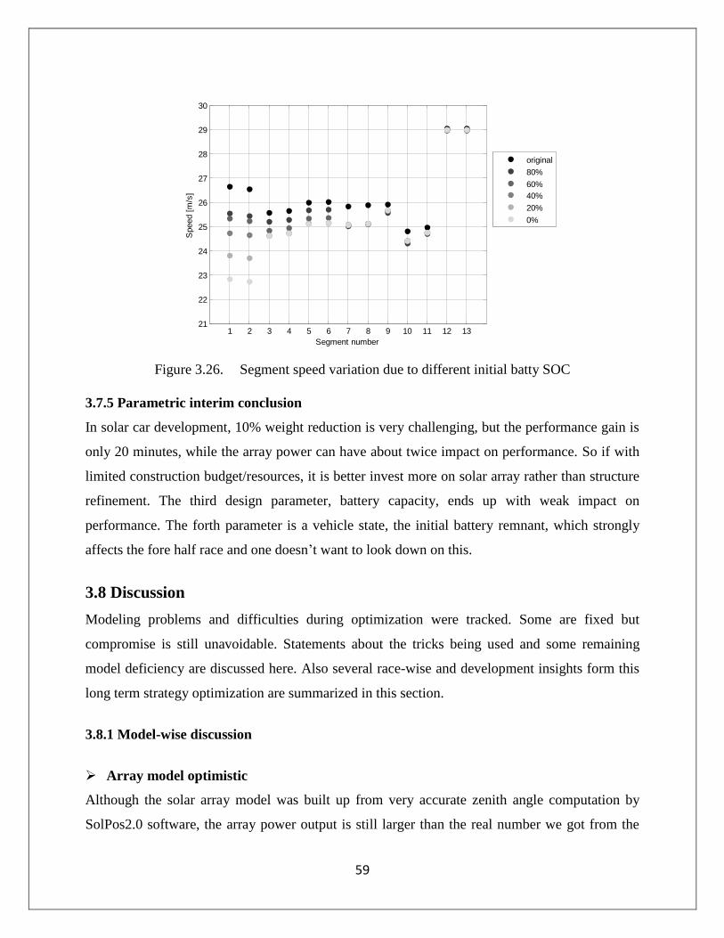
59
Figure 3.26. Segment speed variation due to different initial batty SOC
3.7.5 Parametric interim conclusion
In solar car development, 10% weight reduction is very challenging, but the performance gain is
only 20 minutes, while the array power can have about twice impact on performance. So if with
limited construction budget/resources, it is better invest more on solar array rather than structure
refinement. The third design parameter, battery capacity, ends up with weak impact on
performance. The forth parameter is a vehicle state, the initial battery remnant, which strongly
affects the fore half race and one doesn‟t want to look down on this.
3.8 Discussion
Modeling problems and difficulties during optimization were tracked. Some are fixed but
compromise is still unavoidable. Statements about the tricks being used and some remaining
model deficiency are discussed here. Also several race-wise and development insights form this
long term strategy optimization are summarized in this section.
3.8.1 Model-wise discussion
Array model optimistic
Although the solar array model was built up from very accurate zenith angle computation by
SolPos2.0 software, the array power output is still larger than the real number we got from the
1 2 3 4 5 6 7 8 9 10 11 12 1321
22
23
24
25
26
27
28
29
30
Segment number
Speed [
m/s
]
original
80%
60%
40%
20%
0%

60
solar car team. The empirical equations (3.8) and (3.9) do not well capture the solar array power
output .The speed optimization results is much better than the historical data.The solar car team
participated in the race last year in Australia. Continuum averaged at around 20 m/s in
WSC2007.We have the thirteen optimal cruising speeds average at 25.26 m/s. However, we
believe the solar power output level and trend computed by equation (3.8) and (3.9) is
representative enough for this optimization purpose.
Lack of weather consideration
Weather actually plays an important role in the race especially in American race. We will run
into the rain season in summer time, but the cloud condition is not included into the model. The
sunny weather is one of the assumptions being made for model simplification at beginning of
this subsystem. This is thought to be a major reason that we have optimistic array power output.
Although we could simply include some random clouds to reduce the solar power production . It
is better to keep the model stay in accordance with physics as much as possible instead of
introducing some disturbance to make the model simulation results close to historical data.
Simple meteorology information is under consideration to be included when utilizing this
scheme onto real race this July.
Decision making problem/time dependent modeling
The solar car race strategy is nothing like traditional dimensional design problems, but decision
making problem or control problem. It took some effort to convert the race strategy problem into
the optimization form in our class scope. Also the race strategy strongly entangles with time,
which is also little mentioned in the class, so we also tried hard to come out with the model
having time be included. Gratefully, the results turn out to be good. The objective of a solar
racing car is actually simple, to minimize running time. Having cruising speeds as variables and
battery remnants as constraints turns out to be very good choices that the model actually ends up
in easy function minimization problem after the metamodel was built. The optimization results
and variable behaviors are mapped back to physical quantities and make us able to explain many
intuitive deductions (for example, draining out the battery at the last night of the race) or even
correct some misjudgments.

61
3.8.2 Race-wise discussion
Parametric study on long term performance provides insights for budget allocation
The solar car long term speed performance is strongly related to the solar array rather than other
vehicle parameters (e.g. weight) in real race condition, and the parametric study in this section
quantitatively proved that the maximum array power parameter contributes about three times
objective function (total run time) reduction than the same percentage variation in weight.
Although this conclusion is drawn abruptly because the two parameters physically have different
unit, the run time reduction in array power parametric study was so strongly biased that it‟s clear
that regarding to budget allocation, it is preferred to hold higher priority on array investment than
structural development. This is actually also the truth in real solar car team execution.
It is told from the solar car people that to change those solar array parameters (e.g. enlarge array
area) by a certain percentage, the cost may be ten times higher than to achieve the same
percentage change in structural parameters, but the cost is not included in any of subsystems.
The value of long term strategy optimization
For recent race results, the best team runs almost as twice faster than mediocre teams, and still
there are about half of the participants not able to finish the race within the race time frame; the
solar array matters a lot. However, after the solar array is installed onto the upper shell, the
vehicle structural developments are pretty much done. The important thing that can affect the
race results now falls on to the race strategy, especially long term speed scheduling and battery
scheduling. Before this procedure being conducted, the solar car has raced on empirical
estimations or forward simulations for many generations. No optimization has really been
implemented in race strategy. Now this subsystem development has achieved that the speed
scheduling and battery scheduling are determined with optimization theorem/algorithm
supporting behind the scenes, the battery remnant constraints are retained, and certain optimality
is guaranteed although global optimality is not checked. The battery scheduling is very important
to practical race execution, and is the factor that bothers the strategists the most. In the past, it
mostly depends on the intuition of the strategists to determine the battery remnant for everyday
running, and human judgment goes wrong once in a while. Now the strategy optimization
resolves the battery schedule trouble together while optimizing cruising speeds.

62
As one might recall that one set of feasible cruising speeds was found by hand tuning when
doing metamodel analysis in section 3.5.5, and the fmincon optimization result achieves 43
minutes reduction in total run time. It is not really justifiable to claim how much percentage
improvement has been made here, because the initial guess is just an arbitrary feasible solution.
People may question that we might choose a badly tuned case as baseline on purpose. However,
the value of our work is the significant time reduction which cannot be achieved by hand tuning
the thirteen speed variables simultaneously. Trail-and-error schemes can only improve
performance, but people will not be able to know how far they are away from the optima. This is
also overcome by our work .

63
Subsystem 3: Short term strategy optimization of a solar car – Yogita Pai
4.1. Problem statement
Hills and traffic signals pose an interesting problem in the optimal design of the driving strategy.
The driver has to be alert about where he brakes, accelerates, or coasts when driving over the hill
to minimize the total energy consumption. Different strategies will alter the amount of energy
consumed. If the vehicle travels at too high a speed, more energy will be lost to aerodynamic
drag than necessary. Applying regenerative brakes will put excess energy back into the batteries
and help reduce the total energy consumption. Using the downhill gravitational force will reduce
the energy consumption. All these possibilities will have to be factored into before the realization
of the final goal of the lowest total energy consumption whilst travelling over a hill and passing a
traffic signal.
The short term strategy aims at optimizing the driving strategy in order to minimize the total
amount of energy required to travel over a hill and pass a traffic signal.
Hill scenario
Figure 4.1. Hill scenario
Traffic signal scenario
Figure 4.2. Traffic signal scenario
Based on the reference cruise speed taken
from the long term strategy, the velocity just
before climbing the hill i.e. v1, the velocity at
the top of the hill i.e. v2, the velocity just after
descending the hill i.e.v3, the ahead distance
i.e. x1 and the afterward distance i.e. x2 will
be optimized.
Based on the reference cruise speed taken
from the long term strategy, the braking
distance i.e. x1 and the acceleration
distance i.e. x2 will be optimized.

64
4.2. Nomenclature Symbol Description Unit Type
E
g
ρ
m
Total energy
Acceleration due to gravity
Density of air
Vehicle mass
J
m/s2
kg/m3
kg
Objective
Constant
Constant
Parameter
Crr
Cl
Cd
Coefficient of rolling resistance
Coefficient of Aerodynamic lift
Coefficient of Aerodynamic drag
-
-
-
Parameter
Parameter
Parameter
A
G
vw
vavg
η
Frontal area
Road gradient
Wind velocity
Average or reference vehicle speed
Power train efficiency
-
-
m/s
m/s
-
Parameter
Parameter
Parameter
Parameter
Parameter
D
Da
Dr
F
Pss
Pacc
P
v
a
t
x1
x2
v1
v2
v3
Total drag force
Aerodynamic drag force
Drag force due to rolling resistance
Force applied to the vehicle in the direction of motion
Power required to overcome drag
Power contributing to the acceleration of the vehicle
Power requirement of the vehicle
Velocity of the vehicle
Acceleration / Deceleration of the vehicle
Time
Ahead distance / Braking distance
Afterward distance / Acceleration distance
Velocity just before climbing the hill
Velocity at the tip of the hill
Velocity just after descending the hill
N
N
N
N
W
W
W
m/s
m/s2
sec
m
m
m/s
m/s
m/s
-*
-*
-*
-*
-*
-*
-*
-*
-*
-*
Variable
Variable
Variable
Variable
Variable
*- (dash) means an intermediate calculation term.

65
4.3. Mathematical Model
4.3.1. Objective function
The objective is to optimize the driving strategy in order to minimize the total amount of energy
required to travel over a hill and stop-n-go a traffic signal. The total energy is considered as the
power over a set duration of time which is given by:
𝐸 = 𝑃𝑑𝑡
Here, a positive P corresponds to increasing throttle and a negative P corresponds to regenerative
braking. The power required to propel the vehicle can be split into two components: a steady
state component and an acceleration component.
∴ 𝑃 = 𝑃𝑠𝑠 + 𝑃𝑎𝑐𝑐𝑒𝑙
The power at any time t can be derived from the evaluation of forces applied to the vehicle.
Since
𝐹 = 𝑚𝑎
and
𝑃𝑎𝑐𝑐𝑒𝑙 = 𝐹𝑣
we have
𝑃𝑎𝑐𝑐𝑒𝑙 = 𝑚𝑣𝑎
The forces acting on the car in the steady state condition include the vehicle‟s rolling resistance,
its aerodynamic drag and lift and the gradient of the road surface when moving on a hill [1.3].
Aerodynamic lift can be expressed as:
𝐿𝑖𝑓𝑡 =1
2𝐶𝑙𝐴𝜌𝑣
2
Considering the effect of wind velocity on the vehicle velocity, we have:
𝐿𝑖𝑓𝑡 =1
2𝐶𝑙𝐴𝜌(𝑣 − 𝑣𝑤)2
The rolling resistance can be expressed as:
𝐷𝑟 = 𝑚𝑔 − 𝐿𝑖𝑓𝑡 𝐶𝑟𝑟 = 𝑚𝑔 −1
2𝐶𝑙𝐴𝜌 𝑣 − 𝑣𝑤 2 𝐶𝑟𝑟
Aerodynamic drag can be expressed as:
𝐷𝑎 =1
2𝐶𝑑𝐴𝜌𝑣
2
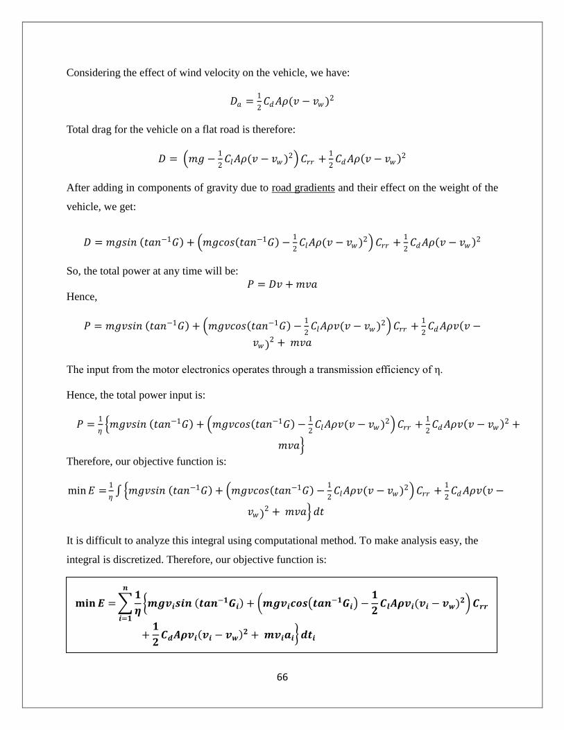
66
Considering the effect of wind velocity on the vehicle, we have:
𝐷𝑎 =1
2𝐶𝑑𝐴𝜌(𝑣 − 𝑣𝑤)2
Total drag for the vehicle on a flat road is therefore:
𝐷 = 𝑚𝑔 −1
2𝐶𝑙𝐴𝜌(𝑣 − 𝑣𝑤 )2 𝐶𝑟𝑟 +
1
2𝐶𝑑𝐴𝜌 𝑣 − 𝑣𝑤 2
After adding in components of gravity due to road gradients and their effect on the weight of the
vehicle, we get:
𝐷 = 𝑚𝑔𝑠𝑖𝑛 𝑡𝑎𝑛−1𝐺 + 𝑚𝑔𝑐𝑜𝑠 𝑡𝑎𝑛−1𝐺 −1
2𝐶𝑙𝐴𝜌(𝑣 − 𝑣𝑤)2 𝐶𝑟𝑟 +
1
2𝐶𝑑𝐴𝜌 𝑣 − 𝑣𝑤 2
So, the total power at any time will be:
𝑃 = 𝐷𝑣 + 𝑚𝑣𝑎 Hence,
𝑃 = 𝑚𝑔𝑣𝑠𝑖𝑛 𝑡𝑎𝑛−1𝐺 + 𝑚𝑔𝑣𝑐𝑜𝑠 𝑡𝑎𝑛−1𝐺 −1
2𝐶𝑙𝐴𝜌𝑣(𝑣 − 𝑣𝑤 )2 𝐶𝑟𝑟 +
1
2𝐶𝑑𝐴𝜌𝑣 𝑣 −
𝑣𝑤 2 + 𝑚𝑣𝑎
The input from the motor electronics operates through a transmission efficiency of η.
Hence, the total power input is:
𝑃 =1
𝜂 𝑚𝑔𝑣𝑠𝑖𝑛 𝑡𝑎𝑛−1𝐺 + 𝑚𝑔𝑣𝑐𝑜𝑠 𝑡𝑎𝑛−1𝐺 −
1
2𝐶𝑙𝐴𝜌𝑣(𝑣 − 𝑣𝑤)2 𝐶𝑟𝑟 +
1
2𝐶𝑑𝐴𝜌𝑣 𝑣 − 𝑣𝑤 2 +
𝑚𝑣𝑎
Therefore, our objective function is:
min 𝐸 =1
𝜂 𝑚𝑔𝑣𝑠𝑖𝑛 𝑡𝑎𝑛−1𝐺 + 𝑚𝑔𝑣𝑐𝑜𝑠 𝑡𝑎𝑛−1𝐺 −
1
2𝐶𝑙𝐴𝜌𝑣(𝑣 − 𝑣𝑤)2 𝐶𝑟𝑟 +
1
2𝐶𝑑𝐴𝜌𝑣 𝑣 −
𝑣𝑤 2 + 𝑚𝑣𝑎 𝑑𝑡
It is difficult to analyze this integral using computational method. To make analysis easy, the
integral is discretized. Therefore, our objective function is:
𝐦𝐢𝐧𝑬 = 𝟏
𝜼 𝒎𝒈𝒗𝒊𝒔𝒊𝒏 𝒕𝒂𝒏−𝟏𝑮𝒊 + 𝒎𝒈𝒗𝒊𝒄𝒐𝒔 𝒕𝒂𝒏
−𝟏𝑮𝒊 −𝟏
𝟐𝑪𝒍𝑨𝝆𝒗𝒊(𝒗𝒊 − 𝒗𝒘)𝟐 𝑪𝒓𝒓
𝒏
𝒊=𝟏
+𝟏
𝟐𝑪𝒅𝑨𝝆𝒗𝒊 𝒗𝒊 − 𝒗𝒘
𝟐 + 𝒎𝒗𝒊𝒂𝒊 𝒅𝒕𝒊
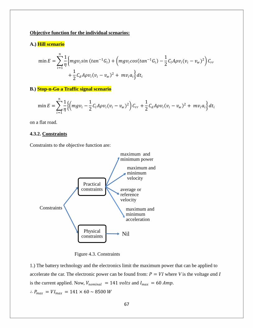
67
Objective function for the individual scenarios:
A.) Hill scenario
min 𝐸 = 1
𝜂 𝑚𝑔𝑣𝑖𝑠𝑖𝑛 𝑡𝑎𝑛−1𝐺𝑖 + 𝑚𝑔𝑣𝑖𝑐𝑜𝑠 𝑡𝑎𝑛
−1𝐺𝑖 −1
2𝐶𝑙𝐴𝜌𝑣𝑖(𝑣𝑖 − 𝑣𝑤 )2 𝐶𝑟𝑟
𝑛
𝑖=1
+1
2𝐶𝑑𝐴𝜌𝑣𝑖 𝑣𝑖 − 𝑣𝑤 2 + 𝑚𝑣𝑖𝑎𝑖 𝑑𝑡𝑖
B.) Stop-n-Go a Traffic signal scenario
min 𝐸 = 1
𝜂 𝑚𝑔𝑣𝑖 −
1
2𝐶𝑙𝐴𝜌𝑣𝑖(𝑣𝑖 − 𝑣𝑤 )2 𝐶𝑟𝑟 +
1
2𝐶𝑑𝐴𝜌𝑣𝑖 𝑣𝑖 − 𝑣𝑤 2 + 𝑚𝑣𝑖𝑎𝑖
𝑛
𝑖=1
𝑑𝑡𝑖
on a flat road.
4.3.2. Constraints
Constraints to the objective function are:
Figure 4.3. Constraints
1.) The battery technology and the electronics limit the maximum power that can be applied to
accelerate the car. The electronic power can be found from: 𝑃 = 𝑉𝐼 where V is the voltage and I
is the current applied. Now, 𝑉𝑛𝑜𝑚𝑖𝑛𝑎𝑙 = 141 𝑣𝑜𝑙𝑡𝑠 and 𝐼𝑚𝑎𝑥 = 60 𝐴𝑚𝑝.
∴ 𝑃𝑚𝑎𝑥 = 𝑉𝐼𝑚𝑎𝑥 = 141 × 60 ~ 8500 𝑊
Constraints
Practical constraints
maximum and minimum power
maximum and minimum velocity
average or reference velocity
maximum and minimum acceleration
Physical constraints Nil
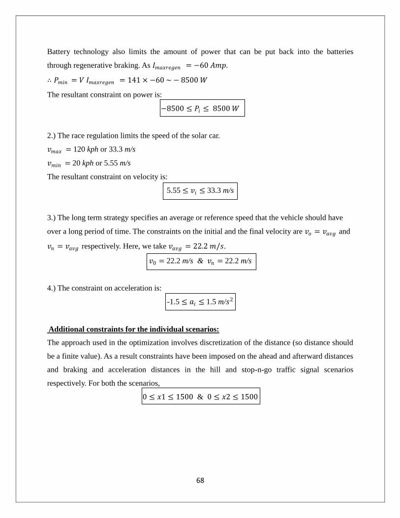
68
Battery technology also limits the amount of power that can be put back into the batteries
through regenerative braking. As 𝐼𝑚𝑎𝑥𝑟𝑒𝑔𝑒𝑛 = −60 𝐴𝑚𝑝.
∴ 𝑃𝑚𝑖𝑛 = 𝑉 𝐼𝑚𝑎𝑥𝑟𝑒𝑔𝑒𝑛 = 141 × −60 ~ − 8500 𝑊
The resultant constraint on power is:
−8500 ≤ 𝑃𝑖 ≤ 8500 𝑊
2.) The race regulation limits the speed of the solar car.
𝑣𝑚𝑎𝑥 = 120 kph or 33.3 m/s
𝑣𝑚𝑖𝑛 = 20 kph or 5.55 m/s
The resultant constraint on velocity is:
5.55 ≤ 𝑣𝑖 ≤ 33.3 m/s
3.) The long term strategy specifies an average or reference speed that the vehicle should have
over a long period of time. The constraints on the initial and the final velocity are 𝑣𝑜 = 𝑣𝑎𝑣𝑔 and
𝑣𝑛 = 𝑣𝑎𝑣𝑔 respectively. Here, we take 𝑣𝑎𝑣𝑔 = 22.2 𝑚/𝑠.
𝑣0 = 22.2 m/s & 𝑣𝑛 = 22.2 m/s
4.) The constraint on acceleration is:
-1.5 ≤ 𝑎𝑖 ≤ 1.5 m/𝑠2
Additional constraints for the individual scenarios:
The approach used in the optimization involves discretization of the distance (so distance should
be a finite value). As a result constraints have been imposed on the ahead and afterward distances
and braking and acceleration distances in the hill and stop-n-go traffic signal scenarios
respectively. For both the scenarios,
0 ≤ 𝑥1 ≤ 1500 & 0 ≤ 𝑥2 ≤ 1500
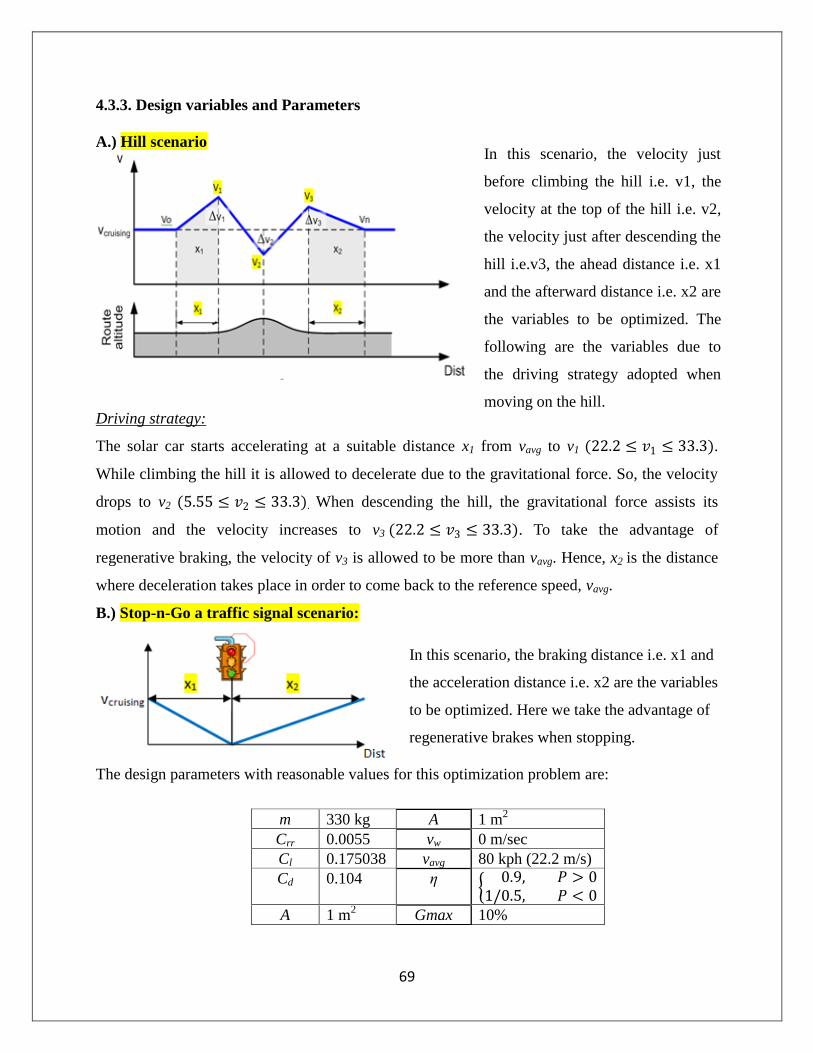
69
4.3.3. Design variables and Parameters
A.) Hill scenario
Driving strategy:
The solar car starts accelerating at a suitable distance x1 from vavg to v1 (22.2 ≤ 𝑣1 ≤ 33.3).
While climbing the hill it is allowed to decelerate due to the gravitational force. So, the velocity
drops to v2 (5.55 ≤ 𝑣2 ≤ 33.3). When descending the hill, the gravitational force assists its
motion and the velocity increases to v3 (22.2 ≤ 𝑣3 ≤ 33.3). To take the advantage of
regenerative braking, the velocity of v3 is allowed to be more than vavg. Hence, x2 is the distance
where deceleration takes place in order to come back to the reference speed, vavg.
B.) Stop-n-Go a traffic signal scenario:
The design parameters with reasonable values for this optimization problem are:
m 330 kg A 1 m2
Crr 0.0055 vw 0 m/sec
Cl 0.175038 vavg 80 kph (22.2 m/s)
Cd 0.104 η
0.9, 𝑃 > 01/0.5, 𝑃 < 0
A 1 m2
Gmax 10%
In this scenario, the velocity just
before climbing the hill i.e. v1, the
velocity at the top of the hill i.e. v2,
the velocity just after descending the
hill i.e.v3, the ahead distance i.e. x1
and the afterward distance i.e. x2 are
the variables to be optimized. The
following are the variables due to
the driving strategy adopted when
moving on the hill.
In this scenario, the braking distance i.e. x1 and
the acceleration distance i.e. x2 are the variables
to be optimized. Here we take the advantage of
regenerative brakes when stopping.

70
4.3.4. Model summary
Hill scenario
Stop-n-Go a traffic signal scenario
min 𝐸 = 1
𝜂 𝑚𝑔𝑣𝑖𝑠𝑖𝑛 𝑡𝑎𝑛−1𝐺𝑖
𝑛
𝑖=1
+ 𝑚𝑔𝑣𝑖𝑐𝑜𝑠 𝑡𝑎𝑛−1𝐺𝑖
−1
2𝐶𝑙𝐴𝜌𝑣𝑖 𝑣𝑖 − 𝑣𝑤 2 𝐶𝑟𝑟
+1
2𝐶𝑑𝐴𝜌𝑣𝑖 𝑣𝑖 − 𝑣𝑤 2
+ 𝑚𝑣𝑖𝑎𝑖 𝑑𝑡𝑖
min 𝐸 = 1
𝜂 𝑚𝑔𝑣𝑖
𝑛
𝑖=1
−1
2𝐶𝑙𝐴𝜌𝑣𝑖 𝑣𝑖 − 𝑣𝑤 2 𝐶𝑟𝑟
+1
2𝐶𝑑𝐴𝜌𝑣𝑖 𝑣𝑖 − 𝑣𝑤 2
+ 𝑚𝑣𝑖𝑎𝑖 𝑑𝑡𝑖
subject to:
𝑎 1, 𝑛 − 1.5 ≤ 0
−𝑎 1, 𝑛 − 1.5 ≤ 0
𝑃 1, 𝑛 − 8500 ≤ 0
−𝑃 1, 𝑛 − 8500 ≤ 0
22.2 − 𝑣1 ≤ 0
𝑣1 − 33.3 ≤ 0
5.55 − 𝑣1 ≤ 0
𝑣1 − 33.3 ≤ 0
22.2 − 𝑣3 ≤ 0
𝑣3 − 33.3 ≤ 0
−𝑥1 ≤ 0
𝑥1 − 1500 ≤ 0
−𝑥2 ≤ 0
𝑥2 − 1500 ≤ 0
subject to:
𝑎 1, 𝑛 − 1.5 ≤ 0
−𝑎 1, 𝑛 − 1.5 ≤ 0
𝑃 1, 𝑛 − 8500 ≤ 0
−𝑃 1, 𝑛 − 8500 ≤ 0
100 − 𝑥1 ≤ 0
𝑥1 − 1000 ≤ 0
100 − 𝑥2 ≤ 0
𝑥2 − 1000 ≤ 0

71
4.3.5. Model analysis
By a mere glance, we observe that by reducing the mass, the coefficient of aerodynamic drag, the
frontal area, the coefficient of rolling resistance and acceleration, the amount of power required
by the car to move at a specified velocity decreases.
As the objective is provided by a highly complicated simulation, monotonicity analysis cannot be
performed. Hence, the constraint activity cannot be determined.
4.4. HILL SCENARIO
4.4.1. Optimization study
The initial optimization study is based on a hill of length 1000m and maximum gradient of 10 %.
4.4.1.1. Discretization:
Figure 4.4. Segment Division
The approach to this problem divides the hill into 4 segments called before climbing AB, when
climbing BC, when descending CD and after descending DE. The aim was to develop a
metamodel using Matlab programming for each of these segments.
The power required can be calculated. Summing the energy at all points gives the total energy
required for motion in each segment.
The individual segments were
discretized into finite grid with
grid size = 0.5 m. Assuming linear
variation of velocity w.r.t.
distance, the velocity can be found
out at each of the discretized
points using similarity of triangles.
Furthermore, the acceleration is
different for each grid.
Figure 4.5. Discretization of segment
AB

72
4.4.1.2. Metamodel generation:
Each segment has 2 variables: 𝐴𝐵 ≡ 𝑥1, 𝑣1 , 𝐵𝐶 ≡ 𝑣1, 𝑣2 , 𝐶𝐷 ≡ 𝑣2, 𝑣3 , 𝐷𝐸 ≡ 𝑣3, 𝑥2 .
Based on different combinations of these variables, we get different energies. For every segment,
more than 6000 such combinations and the corresponding value of energy were obtained. These
values were used to generate a surface fit for each segment as shown in the figure below.
Figure 4.6. Surface fit for (A)x1,v1,E1, (B) v1,v2,E2, (C) v2,v3,E3, (D) x2,v3,E4.
These surfaces were generated using an online tool which also gives the polynomial
approximation to the surface. A full cubic polynomial approximation was used for this purpose.
(D) (C)
(B) (A)

73
The relationship between energy and the variables for individual segments are given below.
%before climbing
E1=(a1+b1*x1+c1*v1+d1*(x1)^2+e1*(v1)^2+f1*(x1)^3+g1*(v1)^3+h1*x1*v1+i1*(x1)^2*v1+j1*x1*(v1)^2)
where
a1 = -8.9096179730351214E+04
b1 = 3.3550475068452783E+01
c1 = -1.4875911962258215E+02
d1 = -1.7322254514067215E-03
e1 = 1.8772653604537641E+02
f1 = -3.2356841002923430E-05
g1 = 2.3237052797142610E-04
h1 = 5.1395937813705217E-01
i1 = 1.0855861821722768E-03
j1 = 1.1402964810445337E-02
%hill climbing
E2=(a2+b2*v1+c2*v2+d2*(v1)^2+e2*(v2)^2+f2*(v1)^3+g2*(v2)^3+h2*v1*v2+i2*(v1)^2*v2+j2*v1*(v2)^2)
where
a2 = 9.0162971045257102E+04
b2 = 8.2744298481203805E+03
c2 = -4.3787635050713325E+03
d2 = -7.4214387536756294E+02
e2 = 6.5704800400868749E+01
f2 = 1.1725362069659374E+01
g2 = 3.5767519648474533E-01
h2 = 5.6312667244938552E+02
i2 = -1.4751389818905363E+01
j2 = 4.4044225410693230E+00
%hill descending
E3=(a3+b3*v2+c3*v3+d3*(v2)^2+e3*(v3)^2+f3*(v2)^3+g3*(v3)^3+h3*v2*v3+i3*(v2)^2*v3+j3*v2*(v3)^2)
where
a3 = 1.1455829434915782E+05
b3 = -1.7519556411221929E+03
c3 = -1.5499465662730792E+04
d3 = -2.4218927623492704E+02
e3 = 3.8751768538788423E+02
f3 = 1.6518426511170361E+00
g3 = 2.8781755367038215E+00
h3 = 4.8051132451072829E+02
i3 = 3.0343553184965435E+00
j3 = -1.4594463103291771E+01
%after descending
E4=(a4+b4*x2+c4*v3+d4*(x2)^2+e4*(v3)^2+f4*(x2)^3+g4*(v3)^3+h4*x2*v3+i4*(x2)^2*v3+j4*x2*(v3)^2)
where
a4 = 5.7951870398372284E+05
b4 = 4.6222780149834853E+02
c4 = -5.9840380855440206E+04
d4 = 8.5489339180245039E-02
e4 = 2.1112314568491197E+03

74
f4 = -1.0797545630109127E-05
g4 = -2.6542209797981897E+01
h4 = -3.1635413444683703E+01
i4 = -2.4125467001529267E-03
j4 = 5.6648021729043241E-01
So the total energy required is given by 𝐸 = 𝐸1 + 𝐸2 + 𝐸3 + 𝐸4. Hence through metamodelling,
we get a new objective function 𝐸 = 𝑓(𝑥1, 𝑣1, 𝑣2 , 𝑣3 , 𝑥2) i.e. energy function in terms of all the
variables.
4.4.1.3. Matlab fmincon optimization and results:
The optimization problem can be restated as:
min 𝐸 = 𝑚𝑖𝑛 𝑓(𝑥1,𝑣1 , 𝑣2, 𝑣3, 𝑥2)
subject to:
22.2 − 𝑣1 ≤ 0
𝑣1 − 33.3 ≤ 0
5.55 − 𝑣1 ≤ 0
𝑣1 − 33.3 ≤ 0
22.2 − 𝑣3 ≤ 0
𝑣3 − 33.3 ≤ 0
−𝑥1 ≤ 0
𝑥1 − 1500 ≤ 0
−𝑥2 ≤ 0
𝑥2 − 1500 ≤ 0
𝑎 1, 𝑛 − 1.5 ≤ 0
−𝑎 1, 𝑛 − 1.5 ≤ 0
𝑃 1, 𝑛 − 8500 ≤ 0
−𝑃 1, 𝑛 − 8500 ≤ 0

75
In spite of reducing the problem, a few hurdles are yet to be overcome. These are the constraints
on acceleration and power at all discretized points. So, for different values of the variables, we
have discretization carried out in the non-linear constraint function. But, because of the way
discretization has been implemented, only the first and the last discretized points of each
segment need to satisfy the acceleration and power constraints.
The result obtained using Matlab fmincon optimization is as follows:
Ahead
distance,
x1* (m)
Velocity just
before climbing
the hill, v1* (m/s)
Velocity at the
top of the hill,
v2* (m/s)
Velocity just
after descending
the hill, v3* (m/s)
Afterward
distance,
x2* (m)
Minimum
energy,
E* (J)
0 22.2 5.55 22.2 0 45480
31.8
5.55
22.2 22.2

76
Figure 4.7. Matlab plots for hill scenario
From the figures, it is clear what the optimization routine would have the driver do.
The optimum values of ahead and afterward distances are 0. This means that the driver need not
accelerate before climbing the hill nor decelerate after descending the hill for minimum energy.
The driver cruises at average speed just before the hill climb. When climbing the hill, the
positive gradient of the hill decelerates the vehicle. Similarly, when descending the hill, its
negative gradient increases its speed.
When moving up the hill its gradient decreases, so the input power required to do work against
the gravity reduces as can be seen in the figure. When moving down the hill its negative gradient
increases. Very little power is utilized by vehicle. In fact at some point due to higher negative
gradient (this may tend to increase the speed of the car beyond the cruising speed), we apply
regenerative brakes.
Min Energy = 45480 J Total time = 83.3 sec

77
The next step is to do a parametric study using the hilly terrain model, and rate the importance of
different parameters in the model on a realistic range. This is very important for the design
because we need to know which aspects of the car have the largest impact on the overall
performance.
4.4.2. Parametric study:
4.4.2.1. Mass
The following parametric study is based on a ±10% mass change of the vehicle. As the mass of
the vehicle reduces, the energy requirement reduces. This result is reasonable, since the vehicle
requires less power to counteract the effects of gravity when driving uphill.
Figure 4.8. Objective variation w.r.t. mass change for hill scenario
4.4.2.2. Gradient of the hill
The maximum gradient was reduced from 10% to 3%. The optimal energy was found to be
35823J with x1*=0, v1*=22.2, v2*=12.9, v3*=22.2, x2*=0 and the time to traverse the hill = 58.4s.
This is consistent with the idea that as the hills become smaller, the more likely the velocity
profile will level off. The power curve obtained is as shown in figure 4.9. When going up the hill,
the driver will be most of the time coasting with a small amount of power applied. When going
down the hill, more power will be required to accelerate to the long term reference cruise speed.
-4000
-3000
-2000
-1000
0
1000
2000
3000
4000
-10 -5 0 (330 kg) 5 10
Ob
ject
ive
ch
ange
(re
lati
ve t
o b
ase
cas
e),
J
Mass change %
Energy requirement
linear variation

78
Figure 4.9. Power v/s Distance for different hill grade
4.4.2.3. Average speed
The following parametric study is based on a ±20% change in the average speed of the vehicle.
For the same maximum gradient, a vehicle climbing at lower average speeds will require more
power to climb the hill. But, when descending the hill, the gravitational assistance may result in
tremendous increase in velocity. To compensate for this effect (so that the velocity increases only
up to the average speed) the driver may have to apply regenerative brakes. At higher average
speeds, the driver will be mostly coasting with a very small amount of power applied when
climbing the hill. But, when descending the hill, more power will be expended to accelerate the
vehicle back to the higher average speed. This description explains figure 4.10. The variation of
energy w.r.t. average speed as shown in figure 4.11. is closely related to these fundamentals.
Further, as average speed increases, the time taken to traverse the hill reduces which is evident in
figure 4.12.
Figure 4.10. Power v/s Distance for various average speeds
-1000
-500
0
500
1000
1500
2000
2500
3000
3500
10%
3%
Hill descending
-2000
0
2000
4000
6000
8000
10000
60 kph
70 kph
80 kph
90 kph
100 kph
Hill climbing
Hill descending Hill climbing

79
Figure 4.11. Objective variation w.r.t. average speed change for hill scenario
Figure 4.12. Total time taken to traverse the hill w.r.t. average speed for hill scenario
-10000
-5000
0
5000
10000
15000
20000
Ob
ject
ive
ch
ange
(re
lati
ve t
o b
ase
cas
e),
J
Average speed change, kph
Energy requirement
Poly. (Energy requirement)
98.990.5
83.377.5 74.9 72.7
0
20
40
60
80
100
120
60 70 80 90 95 100
Toat
l tim
e, s
Average speed, kph
Time to traverse the hill
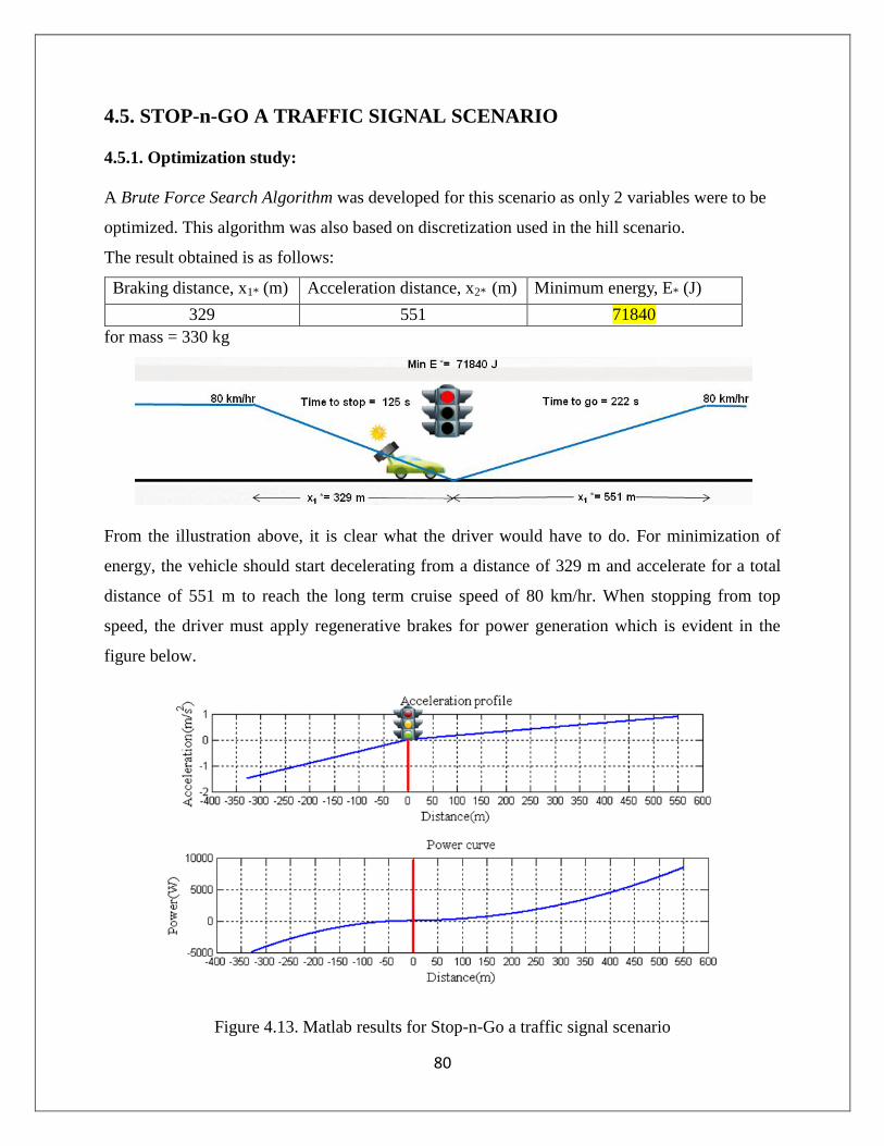
80
4.5. STOP-n-GO A TRAFFIC SIGNAL SCENARIO
4.5.1. Optimization study:
A Brute Force Search Algorithm was developed for this scenario as only 2 variables were to be
optimized. This algorithm was also based on discretization used in the hill scenario.
The result obtained is as follows:
Braking distance, x1* (m) Acceleration distance, x2* (m) Minimum energy, E* (J)
329 551 71840
for mass = 330 kg
From the illustration above, it is clear what the driver would have to do. For minimization of
energy, the vehicle should start decelerating from a distance of 329 m and accelerate for a total
distance of 551 m to reach the long term cruise speed of 80 km/hr. When stopping from top
speed, the driver must apply regenerative brakes for power generation which is evident in the
figure below.
Figure 4.13. Matlab results for Stop-n-Go a traffic signal scenario

81
4.5.2. Parametric study:
4.5.2.1. Mass
When the mass of the vehicle increases, more energy will be generated during regenerative
braking but at the same time, more energy will be expended to accelerate the heavy vehicle.
Figure 4.14. indicates that as the mass increases, more energy will be required. Figure 4.15.
shows the variation of braking and acceleration distance w.r.t. mass change. Figure 4.16. gives
the total time taken to stop-n-go a traffic signal for different mass. The following parametric
study is based on a ±10% mass change of the vehicle.
Figure 4.14. Objective variation w.r.t. mass change for traffic signal scenario
Figure 4.15. Distance w.r.t. mass change for traffic signal scenario
-10000
-8000
-6000
-4000
-2000
0
2000
4000
6000
8000
10000
-10 -5 0(330 kg)
5 10
Ob
ject
ive
ch
ange
(re
lati
ve t
o b
ase
ca
se),
J
Mass change %
Energy requirement
822 850880 909 938
0
100
200
300
400
500
600
700
800
900
1000
-10 -5 0 (330 kg) 5 10
Dis
tan
ce, m
Mass change (relative to base case) %
Total distance to stop-n-go
Braking distance
Acceleration distance

82
Figure 4.16. Total time to stop-n-go w.r.t. mass change
4.5.2.2. Average speed
As the average speed increases, the braking distance and acceleration distance will increase. As a
result, the time to stop and the time to reach the cruising speed increases. Hence, the energy
required increases. This is evident in figure 4.17. The parametric study is based on a ±20%
change in the average speed of the vehicle.
Figure 4.17. Objective variation w.r.t. average speed change for traffic signal scenario
322
334.3
347.9
360.9
374
290
300
310
320
330
340
350
360
370
380
-10 -5 0 (330 kg) 5 10
Toat
l tim
e, s
Mass change %
Total time to stop-n-go
-60000
-40000
-20000
0
20000
40000
60000
80000
Ob
ject
ive
ch
ange
(re
lati
ve t
o b
ase
cas
e),
J
Average speed change, kph
Energy requirement
Poly. (Energy requirement)

83
Figure 4.18. Braking and Acceleration distance variation w.r.t. average speed change
Figure 4.19. Total distance to stop-n-go a traffic signal w.r.t. average speed
-400
-200
0
200
400
600
800
-20 -15 -10 -5 0 5 10 15 20
Bra
kin
g /
Acc
ele
rati
on
dis
tan
ce c
han
ge(r
ela
tive
to
bas
e c
ase
), m
Average speed change, kph
Braking distance
Acceleration distance
404501
603732
880
1050
1247
1475
1719
0
200
400
600
800
1000
1200
1400
1600
1800
2000
60 65 70 75 80 85 90 95 100
Toat
l dis
tan
ce, m
Average speed, kph
Total distance to stop-n-go

84
Figure 4.20. Time variation w.r.t. average speed change for traffic signal scenario
Figure 4.21. Total time to stop-n-go w.r.t. average speed
-150
-100
-50
0
50
100
150
200
250
-20 -15 -10 -5 0 5 10 15 20
Tim
e c
han
ge(r
ela
tive
to
bas
e c
ase
), s
ec
Average speed change, kph
Time to stop
Time to reach cruising speed
192.8226.6
260.5302
347.9
398.8
456.4
521.3
589.4
0
100
200
300
400
500
600
700
60 65 70 75 80 85 90 95 100
Toat
l tim
e, s
Average speed, kph
Total time to stop-n-go

85
4.6. Discussion of results
The goal in this subsystem was to find the optimal driving strategy for the solar car i.e. when
does the driver apply throttle, coast or apply regenerative brakes so as to minimize energy
consumption (E).
The objective function for this optimization is:
min 𝐸 = 1
𝜂 𝑚𝑔𝑣𝑖𝑠𝑖𝑛 𝑡𝑎𝑛−1𝐺𝑖 + 𝑚𝑔𝑣𝑖𝑐𝑜𝑠 𝑡𝑎𝑛
−1𝐺𝑖 −1
2𝐶𝑙𝐴𝜌𝑣𝑖 𝑣𝑖 − 𝑣𝑤 2 𝐶𝑟𝑟
𝑛
𝑖=1
+1
2𝐶𝑑𝐴𝜌𝑣𝑖 𝑣𝑖 − 𝑣𝑤 2 + 𝑚𝑣𝑖𝑎𝑖 𝑑𝑡𝑖
The initial set of parameters and the constraints for this problem gave the minimum energy at
𝑥1, 𝑥2 = 0, 𝑣1 = 22.2, 𝑣2 = 5.55 & 𝑣3 = 22.2 for the hill scenario and 𝑥1 = 329 & 𝑥2 = 551 for
the traffic signal scenario. Less power is used if the driver uses the gravity to add velocity to the
vehicle on the downhill sections of the terrain. Furthermore, the driver may apply regenerative
brakes when stopping.
From the parametric studies, it is evident that the vehicle‟s mass, average speed and road
gradient are very important for the vehicle‟s performance. For a fixed mass, the relationship
between the total energy required and the average speed was established from the parametric
studies. Also the relationship between total time to traverse a hill (also stop-n-go a traffic signal)
and the average speed was obtained. These relationships would be very useful in the system
integration.

86
SECTION 5: System Integration
5.1 Integration architecture
The system integration is a two-step procedure: optimize power income (solar array system) first,
and then optimize power consumption (long term and short term running). The ultimate goal is to
minimize total running time. The two-step integration architecture sketch is shown in Table 5.1. .
Subsystem parametric studies have been preceded and key design variables have been identified,
and minor important design variables (they are parameters to other subsystems) are ruled out
from optimization (kept fixed in system integration). After such design variable elimination
process, the solar array system optimization has only one design variable (concentrator length),
and can be optimized solely to get maximum available solar energy (Evail.). After the solar array
system comes out with the available energy, the second step optimization can start. Long term
strategy will compute cruising speed (Vcruise) based on the optimized available energy and pass
that speed to short term strategy for hill passing and traffic sign passing computation. Both
systems computes time used (TLongTerm and TshortTerm), and a new fmincon problem is formed to
minimize the total running time with cruising speed as design variable.
Solar Array
Long Term Strategy
Short Term Strategy
Eavail.
Vcruise
Minimum Run Time
TLongTerm TShortTerm
Ctr. L. dominates
Array P. dominates
Trf. stop dominates
Solar Array Parametric Study
Long Term Str. Parametric Study
Short Term Str. Parametric Study
Figure 5.1. System integration architecture

87
5.2 Nomenclature
Table 5.1. Integration nomenclature
Symbol Description
m Mass
𝐷 Total distance
𝐷𝑠 Short term distance
𝐷𝑙 Long term distance
𝐷 Distance traversed over the hills
𝐷𝑡 Distance used to stop-n-go a traffic signal
N Number of hills encountered
S Number of traffic signals encountered
L Length of the hill
𝑣𝑎𝑣𝑔 Average speed
T Total time to finish the race
𝑇𝑙 Long term time
𝑇𝑠 Short term time
𝑇 Time to traverse over the hills
𝑇𝑡 Time to stop-n-go traffic signals
E Energy available
𝐸𝑙 Long term energy requirement
𝐸𝑠 Short term energy utilization
𝐸 Energy to traverse over the hills
𝐸𝑡 Energy to stop-n-go traffic signals
5.3 Mathematical model
5.3.1 Array model simplification
In the previous solar array system optimization, the design objective is to maximize the nominal
energy, which is a linear combination of the energy production at point A and point B at a given
date. However, this is not true for the system integration. The power depends on the location
(longitude, latitude), date and time, which means the power production is highly linked to the
long-term strategy. Then, how to handle this problem? Instead of calculating energy in previous
individual subsystem, the power (including charge power, race power and booster power for the
all day) distribution plot with respect to the route and the time of a day for each combination of
the design variables (solar array subsystem) was obtained. Then, the long-term will determine
which segment will be used for racing, which segment will be used for charging, etc.

88
The computation is highly time consuming, thus, previous knowledge about solar array
subsystem design can be employed to eliminate some design variables. The booster module uses
a parabolic mirror concentrator system which can focus 520 mm wide light into 10 mm
concentrator bars. The focus ratio is the largest even considering that the booster module is only
used in charge station. Therefore, the length of the booster (L_bst) can be selected at the upper
bound (it becomes a design parameter) since its „power-to-solar cell area‟ is the best. Next,
considering real world constraint such as concentrator unit and wheel contact avoidance, the
design variable L_tail is fixed at the lower bound (which means that the concentrator is near to
the tail of the car) since it has a little influence in power production and provides more space for
concentrator unit when considering the realization of the concentrator unit. Then the design
variables left are the projected length of the concentrator unit (L_cstr) and the angle (A_cstr)
between the concentrator unit and the horizontal plane. The design variables after simplification
for the solar array are listed in table 5.1.
Table 5.1. Simplified design variables of the solar array
Variable Unit Upper
bound
Lower
bound Levels
L_cstr mm 1100 1400 1100 1180 1260 1320 1400
A_cstr deg 0 12 0 2 4 6 8
In fact, the projected length of the concentrator unit (L_cstr) can also be fixed at the upper bound
because of its strong monotonicity on nominal energy. Even then, the power with respect to
different levels of the length of the concentrator unit was calculated. The result corresponds to
the conclusion of subsystem, i.e. L_cstr should be selected at the upper bound.
Table 5.2. Weight matrix for simplified design variables
L_cstr (mm)\A_cstr (deg) 0 2 4 6 8
1100 26.5 26.5101 26.5403 26.5909 26.6622
1180 27.7 27.7108 27.7432 27.7975 27.8739
1260 28.9 28.9115 28.9462 29.0041 29.0857
1320 29.8 29.8121 29.8483 29.9091 29.9946
1400 31 31.0128 31.0513 31.1157 31.2064

89
The weight matrix for the combination of these design variables is showed in table 5.2 (the base
mass for concentrator unit is 30 Kg). Note that the variation is very small. Thus, we mainly
consider the power production for the selection of solar array design variables.
Figure 5.2. Plot of power with respect to route and time
Figure 5.3. Plot of power with respect to route and time

90
Consider the variation of angle variable, the calculated result for charge power and booster
power are constant because the car is fixed to the sun when under charging. The only complex
result is for race power, under which the car is parallel to the horizontal plane. Figure 5.2 gives
the difference of race power at a given angle and that of zero angle (should be viewed as
electronic version). Recall the route of NASC in figure 2.2, the segment CD is from south to
north and the segment DE is from east to west. Thus, from figure 5.2 and figure 5.3, we know
that it is good to have a small angle (0 deg) for early and late time of the day when the car is
racing in segment CD. For segment DE, it is good to have a large angle in the morning and a
small value in the afternoon. Therefore, it is good to have a mechanism to adjust the angle of the
concentrator unit in real applications. However, for this problem, we cannot have such a
mechanism. To simplify the problem, we select the angle which gives the maximum average race
power. Therefore, we select 8 deg as the angle value for our system integration. The reason
for the upper bound of the angle is 8 deg instead of 12 deg in the subsystem optimization is that
we consider another constraint in real application, i.e. the concentrator unit should never exceed
the upper surface of the car. The constraint is difficult to realize in subsystem design.
Avg(Pwr_race[2deg-0deg]) = 0.0007 KW; Avg(Pwr_race[4deg-0deg]) = 0.0015 KW
Avg(Pwr_race[6deg-0deg]) = 0.0022 KW; Avg(Pwr_race[8deg-0deg]) = 0.0030 KW
Then, we have mass from 330 kg to: m = 331 kg
5.3.2 Integration of long term and short term running
Distance:
Total distance (𝐷) = Long term distance (𝐷𝑙) + Short term distance (𝐷𝑠)
∴ 𝐷𝑙 = 𝐷 − 𝐷𝑠
𝐷 = 2500 miles = 4023360 m
Short term distance (𝐷𝑠) = Distance traversed over the hills (𝐷) + Distance utilized to stop-n-go
traffic signals(𝐷𝑡).
Based on the short term strategy:
Let 𝑑 be the total distance traveled when moving on the hill for minimum energy.
𝑑 = 𝑥1∗ + 𝐿 + 𝑥2∗

91
Since for any case, 𝑥1∗ = 𝑥2∗ = 0
𝑑 = 𝐿 = 1000
∴ 𝐷 = 𝑛 × 𝑑 = 1000 𝑛
Now, 𝑑𝑡 = Braking distance + Acceleration distance
Parametric study (based on mass = 331kg) concerned with the stop-n-go a traffic signal scenario
in the short term strategy gives us relationship between 𝑑𝑡 and 𝑣𝑎𝑣𝑔 .
𝑑𝑡 = 0.2074 𝑣𝑎𝑣𝑔3 − 7.795 𝑣𝑎𝑣𝑔
2 + 152.7𝑣𝑎𝑣𝑔 − 938
∴ 𝐷𝑡 = 𝑠 × 𝑑𝑡 = (0.2074 𝑣𝑎𝑣𝑔3 − 7.795 𝑣𝑎𝑣𝑔
2 + 152.7𝑣𝑎𝑣𝑔 − 938)𝑠
∴ 𝐷𝑠 = 0.2074 𝑣𝑎𝑣𝑔3 − 7.795 𝑣𝑎𝑣𝑔
2 + 152.7𝑣𝑎𝑣𝑔 − 938 𝑠 + 1000 𝑛
∴ 𝐷𝑙 = 4023360 − 0.2074 𝑣𝑎𝑣𝑔3 − 7.795 𝑣𝑎𝑣𝑔
2 + 152.7𝑣𝑎𝑣𝑔 − 938 𝑠 − 1000 𝑛
Time:
The ultimate objective of the solar car is to finish the race in minimum time.
So,
Time to complete the race (𝑇) = Time required to cover the long term distance (𝑇𝑙) + Time
utilized to cover short term distance (𝑇𝑠)
Now
𝑇𝑙 =𝐷𝑙
𝑣𝑎𝑣𝑔
=4023360 − 0.2074 𝑣𝑎𝑣𝑔
3 − 7.795 𝑣𝑎𝑣𝑔2 + 152.7𝑣𝑎𝑣𝑔 − 938 𝑠 − 1000 𝑛
𝑣𝑎𝑣𝑔
Short term time (𝑇𝑠) = Time to traverse over the hills (𝑇) + Time to stop-n-go traffic
signals(𝑇𝑡)
From the parametric study,
𝑡 = 0.08183 𝑣𝑎𝑣𝑔2 − 6 𝑣𝑎𝑣𝑔 + 176.2 / 𝑖𝑙𝑙
𝑡𝑡 = −0.1759 𝑣𝑎𝑣𝑔3 + 12.36 𝑣𝑎𝑣𝑔
2 − 251.6 𝑣𝑎𝑣𝑔 + 1769/𝑠𝑖𝑔𝑛𝑎𝑙
∴ 𝑇 = 𝑛 × 𝑡 = 0.08183 𝑣𝑎𝑣𝑔2 − 6 𝑣𝑎𝑣𝑔 + 176.2 𝑛
& 𝑇𝑡 = 𝑠 × 𝑡𝑡 = −0.1759 𝑣𝑎𝑣𝑔3 + 12.36 𝑣𝑎𝑣𝑔
2 − 251.6 𝑣𝑎𝑣𝑔 + 1769 𝑠
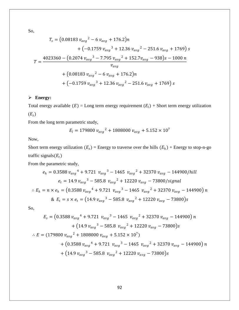
92
So,
𝑇𝑠 = 0.08183 𝑣𝑎𝑣𝑔2 − 6 𝑣𝑎𝑣𝑔 + 176.2 𝑛
+ −0.1759 𝑣𝑎𝑣𝑔3 + 12.36 𝑣𝑎𝑣𝑔
2 − 251.6 𝑣𝑎𝑣𝑔 + 1769 𝑠
𝑇 =4023360 − 0.2074 𝑣𝑎𝑣𝑔
3 − 7.795 𝑣𝑎𝑣𝑔2 + 152.7𝑣𝑎𝑣𝑔 − 938 𝑠 − 1000 𝑛
𝑣𝑎𝑣𝑔
+ 0.08183 𝑣𝑎𝑣𝑔2 − 6 𝑣𝑎𝑣𝑔 + 176.2 𝑛
+ −0.1759 𝑣𝑎𝑣𝑔3 + 12.36 𝑣𝑎𝑣𝑔
2 − 251.6 𝑣𝑎𝑣𝑔 + 1769 𝑠
Energy:
Total energy available (𝐸) = Long term energy requirement (𝐸𝑙) + Short term energy utilization
(𝐸𝑠)
From the long term parametric study,
𝐸𝑙 = 179800 𝑣𝑎𝑣𝑔2 + 1808000 𝑣𝑎𝑣𝑔 + 5.152 × 10⁷
Now,
Short term energy utilization (𝐸𝑠) = Energy to traverse over the hills (𝐸) + Energy to stop-n-go
traffic signals(𝐸𝑡)
From the parametric study,
𝑒 = 0.3588 𝑣𝑎𝑣𝑔4 + 9.721 𝑣𝑎𝑣𝑔
3 − 1465 𝑣𝑎𝑣𝑔2 + 32370 𝑣𝑎𝑣𝑔 − 144900/𝑖𝑙𝑙
𝑒𝑡 = 14.9 𝑣𝑎𝑣𝑔3 − 585.8 𝑣𝑎𝑣𝑔
2 + 12220 𝑣𝑎𝑣𝑔 − 73800/𝑠𝑖𝑔𝑛𝑎𝑙
∴ 𝐸 = 𝑛 × 𝑒 = 0.3588 𝑣𝑎𝑣𝑔4 + 9.721 𝑣𝑎𝑣𝑔
3 − 1465 𝑣𝑎𝑣𝑔2 + 32370 𝑣𝑎𝑣𝑔 − 144900 𝑛
& 𝐸𝑡 = 𝑠 × 𝑒𝑡 = 14.9 𝑣𝑎𝑣𝑔3 − 585.8 𝑣𝑎𝑣𝑔
2 + 12220 𝑣𝑎𝑣𝑔 − 73800 𝑠
So,
𝐸𝑠 = 0.3588 𝑣𝑎𝑣𝑔4 + 9.721 𝑣𝑎𝑣𝑔
3 − 1465 𝑣𝑎𝑣𝑔2 + 32370 𝑣𝑎𝑣𝑔 − 144900 𝑛
+ 14.9 𝑣𝑎𝑣𝑔3 − 585.8 𝑣𝑎𝑣𝑔
2 + 12220 𝑣𝑎𝑣𝑔 − 73800 𝑠
∴ 𝐸 = (179800 𝑣𝑎𝑣𝑔2 + 1808000 𝑣𝑎𝑣𝑔 + 5.152 × 10⁷)
+ 0.3588 𝑣𝑎𝑣𝑔4 + 9.721 𝑣𝑎𝑣𝑔
3 − 1465 𝑣𝑎𝑣𝑔2 + 32370 𝑣𝑎𝑣𝑔 − 144900 𝑛
+ 14.9 𝑣𝑎𝑣𝑔3 − 585.8 𝑣𝑎𝑣𝑔
2 + 12220 𝑣𝑎𝑣𝑔 − 73800 𝑠

93
5.3.3 Model summary
Minimize time
min 𝑇 =4023360 − 0.2074 𝑣𝑎𝑣𝑔
3 − 7.795 𝑣𝑎𝑣𝑔2 + 152.7𝑣𝑎𝑣𝑔 − 938 𝑠 − 1000 𝑛
𝑣𝑎𝑣𝑔
+ 0.08183 𝑣𝑎𝑣𝑔2 − 6 𝑣𝑎𝑣𝑔 + 176.2 𝑛
+ −0.1759 𝑣𝑎𝑣𝑔3 + 12.36 𝑣𝑎𝑣𝑔
2 − 251.6 𝑣𝑎𝑣𝑔 + 1769 𝑠
s.t.
Energy constraint:
179800 𝑣𝑎𝑣𝑔2 + 1808000 𝑣𝑎𝑣𝑔 + 5.152 × 10⁷
+ 0.3588 𝑣𝑎𝑣𝑔4 + 9.721 𝑣𝑎𝑣𝑔
3 − 1465 𝑣𝑎𝑣𝑔2 + 32370 𝑣𝑎𝑣𝑔
− 144900 𝑛
+ 14.9 𝑣𝑎𝑣𝑔3 − 585.8 𝑣𝑎𝑣𝑔
2 + 12220 𝑣𝑎𝑣𝑔 − 73800 𝑠 − 𝐸 ≤ 0
5.3.4 Model analysis
Similar to the long term strategy model analysis, we checked out model monotonicity, and
optimum behaviors of unbounded variables, released constraints, and last constrained
constraints.
5.3.4.1 Monotonicity analysis
The long term running time 0 is conditionally decreasing w.r.t. to design variable cruising speed
within the variable bounds; the short term hill passing time 0 and short term traffic sign passing
time 0 are both increasing, although the hill passing time variation is much small relative to the
other traffic sign passing time as one could see in Figure 5.4. that it is almost a flat line. Further,
long term time decreasing overwhelms the short term time increasing so that the overall run time
is decreasing w.r.t. to design variable, and our hope of having interior optimum won‟t happen.

94
Figure 5.4. Running times of long term and short term events and total race.
5.4 Numerical results
We assume there are 100 hills (n=100) and 100 traffic signs (s=100) in the race route. Parametric
studies on the values of n and s are discussed later.
The optimal cruising speeds and running time results are listed in Table 5.3. , and the time and
energy used by long term and short term running are listed in Table 5.4. and Table 5.5.
respectively. One thing to notice is that the third case bounded and constrained results are the
same as the second case released constraints; they are both bounded optima, which is already
known in monotonicity model analysis in section 5.3.4.1. Also, since energy constraint g1 is not
active in the third case, the solar car won‟t finish with empty battery. Because of the highway
speed limit, solar car cannot run fast enough to completely drain out battery at the finish line.
16 18 20 22 24 26 28 30 320
500
1000
1500
2000
2500
3000
3500
4000
4500
5000
Spd [m/s]
Tim
e [
min
]
Ttot
Tlong
Ttraf
Thill
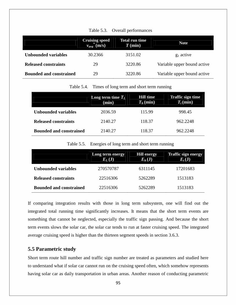
95
Table 5.3. Overall performances
Cruising speed
vavg*
(m/s)
Total run time
T (min) Note
Unbounded variables 30.2366 3151.02 g1 active
Released constraints 29 3220.86 Variable upper bound active
Bounded and constrained 29 3220.86 Variable upper bound active
Table 5.4. Times of long term and short term running
Long term time TL
(min)
Hill time
Th (min)
Traffic sign time
Tt (min)
Unbounded variables 2036.59 115.99 998.45
Released constraints 2140.27 118.37 962.2248
Bounded and constrained 2140.27 118.37 962.2248
Table 5.5. Energies of long term and short term running
Long term energy
EL (J)
Hill energy
Eh (J)
Traffic sign energy
Et (J)
Unbounded variables 270570787 6311145 17201683
Released constraints 22516306 5262289 1513183
Bounded and constrained 22516306 5262289 1513183
If comparing integration results with those in long term subsystem, one will find out the
integrated total running time significantly increases. It means that the short term events are
something that cannot be neglected, especially the traffic sign passing. And because the short
term events slows the solar car, the solar car tends to run at faster cruising speed. The integrated
average cruising speed is higher than the thirteen segment speeds in section 3.6.3.
5.5 Parametric study
Short term route hill number and traffic sign number are treated as parameters and studied here
to understand what if solar car cannot run on the cruising speed often, which somehow represents
having solar car as daily transportation in urban areas. Another reason of conducting parametric

96
study on hill number and traffic sign number is because the only vague short term route
information from we got from the solar car team was just very hilly and full of turns, so we want
to prepare for the worse case and know the limitation of our models (what numbers will make
our program crazy). We explored the hill number (n) and traffic sign number(s) from 0 - 500,
and the results are plotted in Figure 5.5. Figure 5.14. . The baseline case (n=100 and s=100) is
marked with opposite color, so the baseline dot does not apply to the color bar.
While doing the parametric study, we found out many cases are having variable bound active
(see Figure 5.6. , about half plane having speeds same as the baseline case at upper bound), so
several quantities do not change monotonically. For example, one can see the short term stop-
and-go time (Error! Reference source not found.) and energy (Figure 5.12. ) are apparently not
monotonically. However, in general, the total running time is increasing w.r.t. both hill number
and traffic sign number (Table 5.4. ).
0
50
100
150
200
250
300
350
400
450
500
0 100 200 300 400 500
Hill number
Tra
ffic
sig
n n
um
ber
-500
0
500
1000
1500
2000
Base case
Figure 5.5. Objective variation (relative to baseline case)

97
0
50
100
150
200
250
300
350
400
450
500
0 100 200 300 400 500
Hill number
Tra
ffic
sig
n n
um
ber
-10
-9
-8
-7
-6
-5
-4
-3
-2
-1
0
Base case
Figure 5.6. Optimizer (cruise speed) variation (relative to baseline case)
0
50
100
150
200
250
300
350
400
450
500
0 100 200 300 400 500
Hill number
Tra
ffic
sig
n n
um
ber
-200
0
200
400
600
800
1000
1200
Base case
Figure 5.7. Long term time variation
(relative to baseline case)
0
50
100
150
200
250
300
350
400
450
500
0 100 200 300 400 500
Hill number
Tra
ffic
sig
n n
um
ber
-10
-9
-8
-7
-6
-5
-4
-3
-2
-1
0x 10
7
Base case
Figure 5.8. Long term energy variation
(relative to baseline case)

98
0
50
100
150
200
250
300
350
400
450
500
0 100 200 300 400 500
Hill number
Tra
ffic
sig
n n
um
ber
-100
0
100
200
300
400
500
600
Base case
Figure 5.9. Hill time variation
(relative to baseline case)
0
50
100
150
200
250
300
350
400
450
500
0 100 200 300 400 500
Hill number
Tra
ffic
sig
n n
um
ber
-5
0
5
10
15
20
x 106
Base case
Figure 5.10. Hill energy variation
(relative to baseline case)
0
50
100
150
200
250
300
350
400
450
500
0 100 200 300 400 500
Hill number
Tra
ffic
sig
n n
um
ber
-800
-600
-400
-200
0
200
400
600
800
Base case
Figure 5.11. Stop-n-go time variation
(relative to baseline case)
0
50
100
150
200
250
300
350
400
450
500
0 100 200 300 400 500
Hill number
Tra
ffic
sig
n n
um
ber
-1.5
-1
-0.5
0
0.5
1
1.5x 10
7
Base case
Figure 5.12. Stop-n-go energy variation
(relative to baseline case)

99
Figure 5.13. Time variation comparison of long term running, hill passing, traffic sign passing
Figure 5.14. Energy variation comparison of long term running, hill passing, traffic sign
passing
Figure 5.13. and Figure 5.14. especially plot the long term and short term time and energy
together for comparison. The discontinuities on the surfaces are due to the constraint activities
change. One can see that for too large s and n the short term time is almost close to long term
0 100 200 300 400 500 0
200
4000
500
1000
1500
2000
2500
3000
Hill number
Long term
Traf.
Hill
Traffic sign number
0
500
1000
1500
2000
2500
3000

100
time although the energy consumption is still dominated by long term. We are not sure if the race
route has so many short term events that will take up so much time, but the lesson here is the
more often the solar car deviate away from long term cruising speed, the longer the total running
time will be ,which is consistent with intuition.
REFERENCES
[1] Douglas Carroll, “The Winning Solar Car – A Design Guide for Solar Race Car Teams,”
SAE International, 2003, ch. 2.
[2] Jeff Ferman, Jake Ketchum, Ryan Taylor and Blair Willcox, “Investigation into the Projected
Power Yield of a Car-Mounted Solar Concentrator Unit,” The University of Michigan Solar
Car Team Document, 2007.
[3] Peter Pudney, “Optimal energy management for solar-powered cars,” Ph.D. dissertation,
Dept. Applied Math. , Univ. of South Australia, 2000.
[4] UMSolar website, http://www.engin.umich.edu/solarcar/blog/2007/10/continuum-
technology.html, accessed Mar 2007.
[5] Design of Continuum, UM Solar Car Team
[6] D. M. Roche, A. E. T. Schinckel, J. W. V. Storey, C. P. Humphris and M. R. Cuelden, “Speed
of light: The 1996 World Solar Challenge,” Photovoltaics Special Research Centre,
University of New South Wales, Australia, 1997, pp. 43-53.
[7] G. S. Wright, “Optimal Energy Management for Solar Car Race,” Proceedings of the 39th
IEEE Midwest Symposium on Circuits and Systems, Denver, USA, 1996.
[8] Y. Shimizu, Y. Komatsu, M. Torii, and M. Takamuro, “Solar car cruising strategy and its
supporting system,” JSAE Review, vol. 19, pp. 143-149, 1998.
[9] A. Shacklock, M. Duke, N. Burgess, “The 1998 World Solar Rallye: Akita, Japan,” Journal
of Power Sources, vol. 80, pp.199–206, 1998.
[10] NREL SOLPOS 2.0, Solar Position and Intensity,
http://rredc.nrel.gov/solar/codesandalgorithms/solpos/, accessed March 2007.
[12] NOAA ESRL Sunrise/Sunset Calculator,
http://www.srrb.noaa.gov/highlights/sunrise/sunrise.html, accessed March 2007.
[11] Interactive 2-Dimensional and 3-Dimensional Data Modeling, http://zunzun.com/, accessed
March 2007.
[12] “Optimal Driving strategy for a solar electric vehicle” ME 555 final project by Jason
Kramb and Andy Sievers, 2000.