Solar activity over nine millennia: A consistent multi ... · studies were based on individual, sometimes statistically averaged, proxy datasets. Here we aim to provide a new consistent

arX

iv:1

804.

0130

2v1

[as

tro-

ph.S

R]

4 A

pr 2

018

Astronomy & Astrophysics manuscript no. aaa c©ESO 2018April 5, 2018

Solar activity over nine millennia: A consistent multi-proxy

reconstruction

Chi Ju Wu1, I. G. Usoskin2, 3, N. Krivova1, G. A. Kovaltsov4, M. Baroni5, E. Bard5, and S. K. Solanki1, 6

1 Max-Planck-Institut für Sonnensystemforschung, Göttingen, Germany2 Space Climate Research Unit, University of Oulu, Finland3 Sodankylä Geophysical Observatory, University of Oulu, Finland4 Ioffe Physical-Technical Institute, 194021 St. Petersburg, Russia5 CEREGE, Aix-Marseille University, CNRS, Collège de France, Technopôle de l’Arbois, Aix-en-Provence, France6 School of Space Research, Kyung Hee University, Yongin, Gyeonggi-Do,446-701, Republic of Korea

ABSTRACT

Aims. The solar activity in the past millennia can only be reconstructed from cosmogenic radionuclide proxy records in terrestrialarchives. However, because of the diversity of the proxy archives, it is difficult to build a homogeneous reconstruction. All previousstudies were based on individual, sometimes statistically averaged, proxy datasets. Here we aim to provide a new consistent multi-proxy reconstruction of the solar activity over the last 9000 years, using all available long-span datasets of 10Be and 14C in terrestrialarchives.Methods. A new method, based on a Bayesian approach, was applied for the first time to solar activity reconstruction. A Monte Carlosearch (using the χ2 statistic) for the most probable value of the modulation potential was performed to match data from differentdatasets for a given time. This provides a straightforward estimate of the related uncertainties. We used six 10Be series of differentlengths (from 500–10000 years) from Greenland and Antarctica, and the global 14C production series. The 10Be series were resampledto match wiggles related to the grand minima in the 14C reference dataset. The stability of the long data series was tested.Results. The Greenland Ice-core Project (GRIP) and the Antarctic EDML (EPICA Dronning Maud Land) 10Be series diverge fromeach other during the second half of the Holocene, while the 14C series lies in between them. A likely reason for the discrepancyis the insufficiently precise beryllium transport and deposition model for Greenland, which leads to an undercorrection of the GRIPseries for the geomagnetic shielding effect. A slow 6–7-millennia variability with lows at ca. 5500 BC and 1500 AD in the long-term evolution of solar activity is found. Two components of solar activity can be statistically distinguished: the main component,corresponding to the ‘normal’ moderate level, and a component corresponding to grand minima. A possible existence of a componentrepresenting grand maxima is indicated, but it cannot be separated from the main component in a statistically significant manner.Conclusions. A new consistent reconstruction of solar activity over the last nine millennia is presented with the most probable valuesof decadal sunspot numbers and their realistic uncertainties. Independent components of solar activity corresponding to the mainmoderate activity and the grand-minimum state are identified; they may be related to different operation modes of the dynamo.

Key words. Sun:activity - Sun:dynamo

1. Introduction

The Sun is an active star whose magnetic activity varies on dif-ferent timescales, from seconds to millennia. Understanding so-lar variability in detail is important for many reasons, rangingfrom applications in stellar astrophysics and dynamo theory topaleoclimatic and space weather studies. Various direct, partlymultiwavelength spectroscopic solar observations cover the pastfew decades up to a century in the past. They provide knowledgeof the solar variability that is expressed in different indices. Forthe preceding centuries back to 1610, only visual informationfrom simple optical observations in the form of sunspot num-bers (SNs) is available (Hathaway 2015). The quality of the SNseries varies, and the uncertainty increases sufficiently before thenineteenth century (Clette et al. 2014; Usoskin 2017). However,the Maunder minimum in the second half of the seventeenthcentury was observed sufficiently well to conclude that sunspotactivity was exceptionally low (Ribes & Nesme-Ribes 1993;Vaquero et al. 2015; Usoskin et al. 2015). For earlier times, only

indirect proxies can help assessing solar activity 1. Such proxiesare, for example, concentrations of cosmogenic radionuclides ra-diocarbon (14C), beryllium-10 (10Be), or chlorine-36 (36Cl) thatare measured in tree trunks or polar ice cores, respectively. Thesearchives are dated independently. The use of cosmogenic proxiesfor studying the solar activity in the past has been proposed longago (e.g., Stuiver 1961; Stuiver & Quay 1980; Beer et al. 1988),and the method has been developed since then in both measure-ments and modeling (see reviews by Beer et al. 2012; Usoskin2017, and references therein). These data cover timescales of upto ten millennia and more.

Cosmogenic radionuclides are produced as a byproduct ofa nucleonic cascade initiated by galactic cosmic rays (GCR) inthe Earth’s atmosphere. This is the only source of these nuclidesin the terrestrial system (which is why they are called “cos-mogenic”). Radiocarbon 14C is mainly produced as a result ofneutron capture (np−reaction) by nitrogen, which is responsi-ble for > 99% of the natural 14C production. The isotope 10Be

1 Although naked-eye observations of sunspots are available, they donot provide quantitative assessments (Usoskin 2017).

Article number, page 1 of 13

http://arxiv.org/abs/1804.01302v1

A&A proofs: manuscript no. aaa

is produced as a result of spallation reactions of O and N nu-clei caused by energetic GCR particles. After production, thetwo radionuclides have different processes of transport, deposi-tion, and storage in terrestrial archives around the globe. Radio-carbon is mostly measured in dendrochronologically dated an-nual rings of live or dead tree trunks, while 10Be is measuredin glaciologically dated polar ice cores mostly from Greenlandor Antarctica. In addition to the geomagnetic field, the flux ofGCRs impinging on Earth is modulated by large-scale helio-spheric magnetic features (interplanetary magnetic fields and so-lar wind) so that the measured content of the nuclides may serveas a proxy of solar magnetic variability in the past (after the in-fluence of the geomagnetic field has been removed). Differentcosmogenic isotope series exhibit a high degree of similarity ontimescales of a century to a millennium because they share thesame production origin (Bard et al. 1997; Vonmoos et al. 2006;Beer et al. 2012; Usoskin et al. 2009; Delaygue & Bard 2011;Usoskin et al. 2016; Adolphi & Muscheler 2016). However,systematic discrepancies between long-term (multi-millennial)trends in different series can be observed (Vonmoos et al. 2006;Inceoglu et al. 2015; Adolphi & Muscheler 2016; Usoskin et al.2016), probably because of the influence of climate conditions(regional deposition pattern for 10Be or large-scale ocean circu-lation for 14C) or an improper account for the geomagnetic fieldvariation, to which the two isotopes respond differently.

Because of the differences in the isotope records, ear-lier reconstructions of solar activity were obtained basedon individual cosmogenic series, leading to a diversity inthe results. Earlier multi-proxy efforts (e.g., Bard et al. 1997;McCracken et al. 2004; Vonmoos et al. 2006; Muscheler et al.2007; Usoskin et al. 2007; Knudsen et al. 2009) were mostlybased on a simple comparison of individual records. The firstconsistent effort to produce a merged reconstruction was madeby Steinhilber et al. (2012), who used the principle componentanalysis (PCA) to extract the common variability signal (as-sumed to be solar) from the reconstructions based on three cos-mogenic series (global 14C, Antarctic EDML (EPICA DronningMaud Land), and the Greenland Ice-core Project, GRIP, 10Be)and to remove the system effects (e.g., the deposition process,snow accumulation rate, and changes in the carbon cycle anddating uncertainties), which are different for each series. ThePCA method keeps only the relative variability and looses theinformation on the absolute level, which needs further normal-ization. Moreover, this method effectively averages multiple sig-nals without taking the accuracy of each data point and possibletime lags between the signals into account (see Figures S1–S8 inSteinhilber et al. 2012). As discussed by Adolphi & Muscheler(2016), the time mismatch between the 14C and 10Be series maybe as large as 70 years toward the early Holocene, however.

We here introduce a new method for a consistent multi-proxy reconstruction of the solar activity that is based on theBayesian approach to determine the most probable value (andits uncertainties) of the solar activity at any moment in timeby minimizing the χ2-discrepancy between the modeled andthe actually measured cosmogenic isotope data. This methodstraightforwardly accounts for error propagation and providesthe most probable reconstruction and its realistic uncertainties.Since the method is sensitive to the dating accuracy of differentrecords, we redated the 10Be records to match their dating withthat of 14C by applying the standard wiggle-matching method(Cain & Suess 1976; Muscheler et al. 2014) to the official ice-core chronology, as described in Section 3. The solar modulationpotential was assessed using the Bayesian approach from all theavailable datasets (Section 4). Finally, the SN series was calcu-

GMAG.9k

14C

EDML

GRIP

−6760~1900

−6760~1900

−6760~730

−6760~−1650

Dome Fuji

South Pole

NGRIP

Dye3

690~1880

850~1900

1390~1900

1420~1900

−6000 −4000 −2000 0 2000Year (−BC/AD)

Fig. 1. Data series (see Table 1) and temporal coverage. Blue shadingdenotes the cosmogenic isotope series, while green shading shows thegeomagnetic series.

lated (Section 5). Section 6 summarizes our results and conclu-sions.

2. Data

2.1. Cosmogenic isotope records

We here used six 10Be series from Greenland and Antarctica andone global 14C production series, as summarized in Table1 andFigure 1.

The 14C series covers the entire Holocene with homogeneousresolution as given by the globally averaged 14C production ratecomputed by Roth & Joos (2013) from the original International14C Calibration dataset INTCAL09 (Reimer et al. 2009) mea-surements of ∆14C. While this series has a pseudo-annual tempo-ral sampling (Roth & Joos 2013), its true resolution is decadal.The series is provided as an ensemble of 1000 realizations of in-dividual reconstructions. Each realization presents one possiblereconstruction in the sense of a Monte Carlo approach (viz. onerealized path of all possible paths in the parametric space), con-sidering all known uncertainties. This enables directly assessingthe error propagation throughout the entire process.

10Be series have different coverage and temporal resolutions.We reduced them to two cadences. Annual series were keptas they are, while rougher resolved series were resampled todecadal cadence. For each series, we also considered 1000 re-alizations that were synthesized using the mean curve and thestandard deviation (error bars). Two series were updated withrespect to earlier studies. The EDML series was used with thenew Antarctic Ice Core Chronology, version 2012 (AICC2012)(Veres et al. 2013; Bazin et al. 2013). The GRIP series was up-dated from its original ss09(sea) timescale (Johnsen et al. 1995,2001) to the more recent timescale of the Greenland Ice CoreChronology, version 2005 (GICC05) (Vinther et al. 2006).

All 10Be series were converted into units of production/flux[atoms cm−2 sec−1] when possible, which is natural for the iso-tope production by cosmic rays. Originally, 10Be measurementsare given in units of concentration [atoms g−1]. To convert theminto the flux, the independently measured or obtained snow ac-cumulation rate at each site is needed. The accumulation rate


Chi Ju Wu et al.: Solar activity over nine millennia: A consistent multi-proxy reconstruction

was considered individually for each ice core, using the samechronology as for the 10Be data (Veres et al. (2013); Bazin et al.(2013) for EDML on AICC2012 and Rasmussen et al. (2014);Seierstad et al. (2014) for GRIP on the GICC05 timescale). Forthe Dye-3 and South Pole series, accumulation data are not pro-vided, and in these cases, we used concentration data assumingthat the concentration is proportional to the depositional flux,with the scaling factor being a free parameter (Table 1).

2.2. Geomagnetic data

As the geomagnetic data for the last millennia, we used therecent archeo/paleomagnetic model GMAG.9k of the virtualaxial dipole moment (VADM) as published by Usoskin et al.(2016) for the period since ca. 7000 BC. This model pro-vides an ensemble of 1000 individual VADM reconstructionsthat include all the uncertainties. The range of the ensemblereconstruction covers other archeo- and paleomagnetic mod-els (e.g., Genevey et al. 2008; Knudsen et al. 2008; Licht et al.2013; Nilsson et al. 2014; Pavón-Carrasco et al. 2014), as isshown in Figure 2 of Usoskin et al. (2016), which means that therelated uncertainties are covered. The length of the geomagneticseries limits our study to the period since 6760 BC.

3. Data processing

3.1. Temporal synchronization of the records: wigglematching

While the radiocarbon is absolutely dated via dendrochronol-ogy by tree-ring counting, dating of ice cores is less precise. Inprinciple, dating of ice cores can be done, especially on shorttimescales, by counting annual layers of sulfate or sodium whenthe accumulation and the characteristics of the site allow it (e.g.,Sigl et al. 2015). In practice, however, dating of long series isperformed by applying ice-flow models between tie points thatare related to known events, such as volcano eruptions that leaveclear markers in ice. While the accuracy of dating is quite goodaround the tie points, the exact ages of the samples betweenthe tie points may be rather uncertain. This ranges from severalyears during the last millennium to up to 70–100 years in the ear-lier part of the Holocene (Muscheler et al. 2014; Sigl et al. 2015;Adolphi & Muscheler 2016).

Since our method is based on the minimization of the χ2-statistics of all series for a given moment in time, it is crucial thatthese series are well synchronized. Accordingly, we performeda formal synchronization of the series based on the wiggle-matching procedure, which is a standard method for synchro-nizing time series (e.g., Cain & Suess 1976; Hoek & Bohncke2001; Muscheler et al. 2014). We took the 14C chronology as thereference and adjusted the timing of all other series to it.

3.1.1. Choice of wiggles

Since cosmogenic isotope series exhibit strong fluctuations ofvarious possible origins, it is important to match only those wig-gles that can presumably be assigned to the production changes,that is, cosmic ray (solar) variability, and exclude possible re-gional climate spells. One well-suited type of wiggles is relatedto the so-called grand minima of solar activity, which are char-acterized by a fast and pronounced drop in solar activity for sev-eral decades. The most famous example of a grand minimumis the Maunder minimum, which occurred between 1645–1715(Eddy 1976; Usoskin et al. 2015). Grand minima can be clearly

Fig. 2. Typical example of a wiggle in the 14C (red) series comparedwith the original EDML 10Be series (dashed black, scaled up by a factorof 172). Solid and dashed vertical lines denote the middle and the spanof the wiggle considered for 14C. The black sold curve shows the EDML10Be series after the synchronization (see Sect. 3.1.2).

identified in the cosmogenic isotope records as sharp spikes(Usoskin et al. 2007; Inceoglu et al. 2015). A typical (althoughnot the most pronounced) example of such wiggles (grand min-ima) is shown in Figure 2 for the (scaled) original EDML 10Beseries in a dashed curve along with the 14C production data inred. Although the overall variability of the two series looks sim-ilar, the mismatch in the timing between them is clear and isroughly a few decades.

For the further analysis, we selected periods with clear wig-gles (spikes, corresponding to grand minima, as listed in earlierworks – see references in the notes to Table 2) in the 14C seriesas listed in Table 2, along with their centers and time span.

3.1.2. Synchronization of the wiggles

For all the selected wiggles (Table 2), we found the best-fit timeadjustment dT between the analyzed 10Be and the reference 14Cproduction series by maximizing the cross correlation betweenthe series, calculated within a time window centered at the mid-dle of the wiggle. The data were annually interpolated withinthe time windows so that the time step in defining dT was oneyear. The length of the correlation window was chosen as twicethe length of the wiggle (see Table 2). For each wiggle, we re-peatedly calculated the Pearson linear correlation coefficients be-tween the 14C and 10Be series, and we selected the value of dTthat maximized the cross-correlation coefficient R between thetwo series. The standard error (serr) of the correlation coefficientwas calculated using the approximate formula (e.g., Cohen et al.2003):

serr =

√

1 − R2c

n − 2, (1)

where Rc is the maximum correlation coefficient and n is thenumber of the data points within the correlation window. Thisuncertainty serr was translated into the 1σ confidence intervalfor dT , as illustrated in Figure 3, which shows the correlationcoefficient, R (black curve), as a function of the time shift dT .It reaches its maximum Rc = 0.86 at dT = −25 years, as indi-cated by the vertical solid line. The dotted lines bound the 68%confidence interval for dT defined as R = Rc − serr.



Table 1. Temporal coverage, cadence, type of data (production rate, PR; depositional flux, D; or concentration, C) and the resulting best-fit scalingfactors, κ (Section 4), of the cosmogenic isotope series.

Series Location Period (-BC/AD) Cadence Data κ Reference‡

14C: INTCAL09 Global -8000 – 1950 Decadal PR – RJ201310Be: GRIP Greenland -7375 – 1645 Decadal † D 1.028 Yea1997, Mea2004, Vea200610Be: EDML Antarctica -7440 – 730 Decadal † D 0.815 Sea201210Be: NGRIP Greenland 1389 – 1994 Annual D 0.87 Bea200910Be: Dye3 Greenland 1424 – 1985 Annual C 94.4 Bea1990, Mcea200410Be: Dome Fuji (DF) Antarctica 690 – 1880 5-year † D 0.87 Hea200810Be: South Pole (SP) Antarctica 850 – 1960 Decadal C 342.2 Rea1990, Bea1997† Resampled to decadal resolution.‡ References: RJ2013 (Roth & Joos 2013); Yea1997 (Yiou et al. 1997); Mea2005 (Muscheler et al. 2004); Mcea2004(McCracken et al. 2004); Vea2006 (Vonmoos et al. 2006); Sea2012 (Steinhilber et al. 2012); Bea2009 (Berggren et al. 2009);Bea1990 (Beer et al. 1990); Hea2008 (Horiuchi et al. 2008); Rea1990 (Raisbeck et al. 1990); Bea1997 (Bard et al. 1997).

Table 2. Wiggles (central date and the length in years) used for synchronization of the various 10Be time series to 14C (Eddy 1976; Stuiver & Quay1980; Stuiver & Braziunas 1989; Goslar 2003; Inceoglu et al. 2015; Usoskin et al. 2016), and the synchronization time (in years) for the GRIP andEDML series. All dates are given in -BC/AD for dendrochronologically dated 14C.

Date Length dT (EDML) dT (GRIP) Date Length dT (EDML) dT (GRIP)

1680 80 N/A N/A -3325 90 −20+10−11

7+6−7

1480 160 N/A 8+5−6

-3495 50 −23+6−7

6+6−6

1310 80 N/A 2+4−5

-3620 50 −26+21−10

5+6−6

1030 80 N/A 0+4−4

-4030 100 −19+6−6

2+5−4

900 80 N/A 13+4−3

-4160 50 −22+5−6

−3+5−5

690 100 16+8−6

−1+5−5

-4220 30 −24+5−5

−6+5−5

260 80 12+7−6

0+5−4

-4315 50 −26+4−5

4+3−3

-360 120 6+5−6

2+6−3

-5195 50 −19+4−5

7+5−5

-750 70 −18+12−9

0+2−5

-5300 50 −18+4−5

7+5−5

-1385 80 −25+9−7

3+4−5

-5460 40 −22+5−5

18+5−4

-1880 80 −30+7−6

5+6−6

-5610 40 −36+9−4

29+7−8

-2120 40 −27+5−6

6+7−6

-5970 60 −29+14−8

20+6−6

-2450 40 −28+4−5

0+4−3

-6060 60 −27+13−9

15+6−8

-2570 100 −29+4−4

0+3−3

-6385 130 −22+10−11

−4+6−14

-2855 90 −20+7−6

−14+16−10

-6850 100 −19+7−7

−24+8−7

-3020 60 −18+6−8

−7+12−9

-7030 100 −25+6−6

−39+8−12

-3080 60 −32+6−6

−4+11−9

-7150 100 −29+5−5

−49+8−15

Fig. 3. Example of the calculation of the best-fit time adjustment dT =−25 years (solid vertical line) and its 68% confidence interval (dashedlines, -31 and -19 years) for the wiggle case shown in Figure 2. ThePearson linear correlation was calculated between the 14C and EDML10Be series for the ±100-year time window around the center of thewiggle.

The ‘momentary’ time adjustments dT were considered as‘tie points’ (listed in Table 2) for the 10Be series, with a linearinterpolation used between them. Adjustments for the EDML

series, based here on a new Antarctic Ice Core Chronology(AICC2012; Veres et al. 2013), lie within +20/-40 years, whilefor the GRIP series, they vary within +20/-50 years. The adjust-ment range for GRIP is concordant with the Greenland chronol-ogy correction function (e.g., Muscheler et al. 2014) within theuncertainties of the GICC05 timescale (Seierstad et al. 2014).Some discrepancies may be caused by the differences in thedatasets and applied method. There are no earlier results for theEDML synchronization chronology to be compared with. Weemphasize here that we do not pretend to perform a full chrono-logical scale update, but only to match wiggles between a singleberyllium series and 14C data, which is sufficient for this work. Inparticular, earlier synchronization studies produced smooth cor-rection curves (e.g., Knudsen et al. 2009; Muscheler et al. 2014),where individual wiggles may still be slightly mismatched, whilewe are focused here on matching each wiggle in each series sep-arately.

An example of the resulting redated 10Be series compared tothe reference 14C record is shown with the solid black curve inFigure 2. The synchronization obviously improves the cross cor-relation between the series, as shown in Table 3. The improve-ment (in terms of the ratio of R2, which is a measure of the power



Table 3. Squared correlation coefficients between the six 10Be seriesand the 14C series for the originally dated (Ro) and synchronized (Rs)series. The improvement factor f is defined as the ratio of the squaredcorrelation coefficients.

GRIP EDML NGRIP Dye3 DF SP

R2o 0.60 0.18 0.12 0.23 0.57 0.53

R2s 0.66 0.38 0.14 0.26 0.59 0.53

f 1.11 2.14 1.11 1.14 1.03 1.01

of covariability between the original and synchronized series) issignificant for the long (1.1 and 2.14 for the GRIP and EDMLseries, respectively) and shorter Greenland series (NGRIP andDye3), but small for the short Antarctic series.

The pairwise wavelet coherence between long-term series isshown in Figure 4, calculated following the procedure describedin Usoskin et al. (2009), including the significance estimate us-ing the non-parametric random-phase method (Ebisuzaki 1997).The coherence between EDML 10Be and 14C series (panel a)is good on timescales shorter than 1000 years and insignificanton timescales longer than 2000–3000 years, with no coherencein between. The coherence between the GRIP 10Be and 14C se-ries is good at all timescales longer than 400–500 years. The co-herence between the GRIP and EDML series is intermittent ontimescales shorter than 1000 years and insignificant on longertimescales.

4. Reconstruction of the solar modulation potential

Since cosmogenic isotopes are produced by cosmic rays in theEarth’s atmosphere (Beer et al. 2012), their measured produc-tion/depositional flux reflects changes in the cosmic ray fluxin the past. In turn, cosmic rays are modulated by solar mag-netic activity, which is often quantified in terms of the modu-lation potential φ. The latter is a useful parameter to describethe solar modulation of GCRs using the so-called force-fieldparametrization formalism (e.g., Caballero-Lopez & Moraal2004; Usoskin et al. 2005). In an ideal case, when both the pro-duction rate of cosmogenic isotopes and the geomagnetic field ata given time are known, the corresponding modulation parametercan be calculated for the given isotope using a production modelthat considers in great detail all the processes of the nucleonic-muon-electromagnetic cascade that are triggered by energeticcosmic rays in the atmosphere. Here we used the productionmodel by Poluianov et al. (2016), which is a recent update ofthe widely used cosmic ray atmospheric cascade model (CRAC;Kovaltsov & Usoskin 2010; Kovaltsov et al. 2012). This modelprovides absolute production rates and is in full agreementwith other modern models (Pavlov et al. 2017). The modu-lation potential φ is defined here (see the full formalism inUsoskin et al. 2005) for the local interstellar spectrum accord-ing to Burger et al. (2000). Since the modulation potential is amodel-dependent parameter, our result cannot be directly com-pared to the φ−values based on different assumptions (e.g.,Steinhilber et al. 2012) without a recalibration (Herbst et al.2010; Asvestari et al. 2017). Thus, the φ−series is an interme-diate result that is further converted into an physical index of theopen magnetic flux and subsequently into the SNs.

The relation between the isotope production rate and its mea-sured content (∆14C for 14C and depositional flux or concentra-tion for 10Be) depends on the corresponding atmospheric or ter-restrial cycle of the isotope. Radiocarbon is involved, as carbon-dioxide gas, in the global carbon cycle and is almost completely

a) EDML-vs-14C

Pe

rio

d (

Ye

ars

)

Time-6000 -5000 -4000 -3000 -2000 -1000 0

64

128

256

512

1024

2048

4096

b) GRIP-vs-14C

Pe

rio

d (

Ye

ars

)

Time-6000 -5000 -4000 -3000 -2000 -1000 0

64

128

256

512

1024

2048

4096

c) GRIP-vs-EDML

Pe

rio

d (

Ye

ars

)

Time-6000 -5000 -4000 -3000 -2000 -1000 0

64

128

256

512

1024

2048

4096

0.0

0.2

0.4

0.6

0.8

1.0

Fig. 4. Wavelet coherence between long series, redated using the wigglematching, considered here: (a) 10Be EDML vs. 14C, (b) 10Be GRIP vs.14C, and (c) 10Be GRIP vs. 10Be EDML. The color scale ranges from 0(deep blue) to 1 (dark red). Arrows denote the relative phasing betweenthe series: arrows pointing right denote phase matching, while arrowspointing left show the antiphase. The white curves denote the cone ofinfluence (COI) beyond which the result is unreliable.

mixed and homogenized over the global hemisphere. Here weused the globally averaged 14C production rate as computed byRoth & Joos (2013) from the INTCAL09 standard ∆14C dataset



(Reimer et al. 2009) using a new-generation dynamic carboncycle model that includes coupling with the diffusive ocean.However, the effect of extensive fossil fuel burning (Suess ef-fect) makes it difficult to use 14C data after the mid-ninteenthcentury because of large and poorly constrained uncertainties(Roth & Joos 2013). Radiocarbon data cannot be used after the1950s because of man-made nuclear explosions that led to mas-sive production of 14C. Accordingly, we did not extend our anal-ysis to the twentieth century (cf., e.g., Knudsen et al. 2009).

In contrast to 14C, 10Be is not globally mixed, and itstransport or deposition in the atmosphere is quite complicatedand subject to local and regional conditions. Here we appliedthe 10Be production model by Poluianov et al. (2016), and at-mospheric transport and deposition were considered via theparametrization by Heikkilä et al. (2009, 2013), who performeda full 3D simulation of the beryllium transport and deposition inthe Earth’s atmosphere. However, the existing models consideronly the large-scale atmospheric transport and do not addressin full detail the deposition at each specific location; this maydiffer significantly from site to site. This remains an unknownfactor (up to 1.5 in either direction) between the modeled andactually measured deposition flux of 10Be at any given location(e.g., Sukhodolov et al. 2017). On the other hand, a free conver-sion factor exists if the 10Be data are provided in concentrationunits rather than depositional flux. Therefore, we considered asingle scaling factor that enters the production rate Q so that itmatches the measured values. This factor was adjusted for each10Be series separately.

Sporadic solar energetic particle (SEP) events are sometimesproduced by the Sun, with strong fluxes of energetic particlesimpinging on the Earth’s atmosphere. Although these solar par-ticle storms usually have a short duration and soft energy spec-trum, the SEP flux can produce additional cosmogenic isotopesin the atmosphere. For extreme events, the enhancement of theisotope production may greatly exceed the annual yield fromGCR (Usoskin & Kovaltsov 2012). If not properly accountedfor, these events may mimic periods of reduced solar activity(McCracken & Beer 2015), since the enhanced isotope produc-tion is erroneously interpreted in terms of the enhanced GCRflux, and consequently, in terms of reduced solar activity. Twoextreme SEP events are known that can lead to such an erroneousinterpretation (Bazilevskaya et al. 2014): the strongest event oc-curred around 775 AD (Miyake et al. 2012), and a weaker eventwas reported in 994 AD (Miyake et al. 2013). The energy spec-tra of these events have been assessed elsewhere (Usoskin et al.2013; Mekhaldi et al. 2015). The production effect of the eventon the 10Be data in polar ice was calculated by Sukhodolov et al.(2017) and removed from the original data. One potential candi-date around 5480 BC studied by Miyake et al. (2017) appears tobe an unusual solar minimum rather than an SEP event. Accord-ingly, we kept it as a wiggle and did not correct for the possibleSEP effect.

Here we first calculated the modulation potential φ in the pastfor each series individually, and then for all series together. Thereconstruction process is described in detail below.

4.1. Reducing the series to the reference geomagneticconditions

The temporal variability of cosmogenic isotope production con-tains two signals: solar modulation, and changes in geomagneticfield. These signals are independent of each other and can thus beseparated. Since here we are interested in the solar variability, weremoved the geomagnetic signal by reducing all production rates

Fig. 5. (a) Original (black) mean 14C production rate (Roth & Joos2013) and the one reduced to the standard geomagnetic conditions (red).(b) mean VADM reconstruction (Usoskin et al. 2016).

to the reference geomagnetic conditions, defined as follows: thegeomagnetic field is dipole-like, aligned with the geographicalaxis, and its virtual axial dipole moment (VADM) is 8 × 1022 Am2. The exact VADM value is not important for the procedure,therefore we chose a rounded value close to the mean value forthe twentieth century. The reduction was made in two steps:

(1) From the given isotope production rate Q(t) and the geomag-netic VADM M(t), we calculated the value of φ(t) using theproduction model by Poluianov et al. (2016).

(2) From the value of φ(t) computed in step 1, we calculatedthe reduced production rate Q∗(t) using the same productionmodel, but now fixing the VADM at M = 8 × 1022 A m2.This value roughly corresponds to conditions in the twentiethcentury. This yields the isotope production rate as it wouldhave been during time t if the geomagnetic field had beenkept constant at this value of M.

The new Q∗ series is now free (in the framework of the adoptedmodel) of the geomagnetic changes and is used in the subse-quent reconstructions. An example of the original series and theseries corrected for variations in the geomagnetic field is shownin Figure 5.

4.2. Reconstruction based solely on 14C

First, we calculated the solar modulation potential based solelyon the radiocarbon data using a Monte Carlo method similar tothe method developed by Usoskin et al. (2014, 2016). The re-construction includes the following steps:

(1) For each moment t in time, we used 1000 realizations Qi(t)of the full ensemble provided by Roth & Joos (2013). Theserealizations include uncertainties of the carbon cycle and ofthe measurement errors. At the same time, we also used 1000realizations of the VADM M j(t) from Usoskin et al. (2016),which include uncertainties and cover the range of availablearcheomagnetic reconstructions to calculate 106 values of



Fig. 6. Example of the χ2 vs. φ dependence for 805 AD for the 14Cseries. The dashed lines represent the 68% confidence interval for φ.

Fig. 7. Series of the modulation potential φ computed based only on the14C data. Shading denotes the 68% confidence interval.

Q∗i j

(t), as described in Section 4.1. The whole ensemble pro-

vides a natural way to represent the range and uncertaintiesof the reconstructed quantities (Q or VADM). For this Q∗

i j(t)

ensemble, we calculated the mean 〈Q∗(t)〉 and the standarddeviation σQ(t).

(2) Using the statistics of the Q∗(t) ensemble, we defined foreach time t, the best-fit φ(t) that minimizes the value of χ2:

χ2(φ) =

(

〈Q∗〉 − Q′(φ)

σQ

)2

, (2)

where Q′(φ) is the value of Q∗ computed for a given valueof φ, which was scanned over the range 0 – 2000 MeV. Thebest-fit value of φ0 is defined as the value corresponding tothe minimum χ2

0(→ 0 for a single series used). The 68% con-

fidence interval of φ is defined as the interval bounded by thevalues of χ2 = χ2

0+ 1. An example of the χ2(φ) dependence

and definition of the best-fit φvalues and its uncertainties isshown in Figure 6.

(3) The series of reconstructed φ based on 14C (φ14C) was thencomputed, along with the uncertainties, as shown in Fig. 7.

4.3. Comparison between the long 10Be and 14C series

Next we compared the long-term behavior, in the sense of thescaling factors, of the long-running 10Be series versus the ref-erence 14C series. First we considered a 1000-year window and

Fig. 8. The 10Be scaling factor κ, with 68% uncertainties indicated bythe grey shading, in the sliding 1000-year window as a function of time.Panels a and b are for the GRIP and EDML series, respectively. Dashedlines depict the κ factor defined for the entire period (Section 4.5).

calculated the mean value of 〈φ14C〉 within this period, as de-scribed in Section 4.2. We then scaled each 10Be series individu-ally with a scaling factor κ and reconstructed the value of φκ forthe rescaled 10Be series in this time window. The value of κ wasdefined such that the mean value of φ10Be agrees with the valuefor 14C for the same period, that is, 〈φ10Be〉 = 〈φ14C〉. Then, the1000-year window was moved by 100 years and the procedurewas repeated. The resulting 10Be scaling factors κ are shown asa function of time in Figure 8.

The κ-factor for the GRIP series is relatively stable duringthe period 6760 BC – 3000 BC and depicts a steady monotonousdecrease around 3000 BC and reaching -12% with respect to thefinal κGRIP around 1000 AD. The Pearson squared correlationbetween the two curves is significant, R2 =0.78 (p−value 0.02)2 , implying a possible residual effect of the geomagnetic field inthe reconstruction.

It is interesting to note that the two 10Be series show verydifferent trends during the second half of the Holocene. The κ-factor for the EDML series shows a weak growing trend againstthe 14C series over the entire period of their overlap, with κ vary-ing from -5% to +10%. A shallow wavy variability can be no-ticed, with a quasi-period of approximately 2400 years, whichis probably related to the Hallstatt cycle (Damon & Sonett 1991;Usoskin et al. 2016). The correlation between the κ−factor forEDML and the VADM is insignificant R2 = 0.52 (p = 0.12).This suggests that the under-corrected geomagnetic field effectis most likely only related to the GRIP series.

The discrepancy between GRIP and 14C series is well known(e.g., Vonmoos et al. 2006; Inceoglu et al. 2015), but has typi-cally been ascribed to the early part of the Holocene becauseboth series are normalized to the modern period. With this nor-malization, the records agree with each other over the last mil-lennia but diverge before ca. 2000 BC (Inceoglu et al. 2015).This discrepancies has sometimes (e.g., Usoskin 2017, and ref-

2 The significance is estimated using the non-parametric random-phasemethod by Ebisuzaki (1997).



erences therein) also been explained as a possible delayed effect(not perfectly stable thermohaline circulation) of the deglacia-tion in the carbon cycle (e.g., Muscheler et al. 2004). However,as we show here, this explanation is unlikely for two reasons.

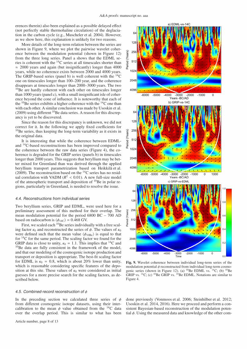
More details of the long-term relation between the series areshown in Figure 9, where we plot the pairwise wavelet coher-ence between the modulation potential (shown in Figure 12)from the three long series. Panel a shows that the EDML se-ries is coherent with the 14C series at all timescales shorter than≈ 2000 years and again (but insignificantly) longer than 4000years, while no coherence exists between 2000 and 4000 years.The GRIP-based series (panel b) is well coherent with the 14Cone on timescales longer than 100–200 year, and the coherencedisappears at timescales longer than 2000–3000 years. The two10Be are hardly coherent with each other on timescales longerthan 1000 years (panel c), with a small insignificant isle of coher-ence beyond the cone of influence. It is noteworthy that each ofthe 10Be series exhibits a higher coherence with the 14C one thanwith each other. A similar conclusion was made by Usoskin et al.(2009) using different 10Be data series. A reason for this discrep-ancy is yet to be discovered.

Since the reason for this discrepancy is unknown, we did notcorrect for it. In the following we apply fixed coefficients for10Be series, thus keeping the long-term variability as it exists inthe original data.

It is interesting that while the coherence between EDML-and 14C-based reconstructions has been improved compared tothe coherence between the raw data series (Figure 4), the co-herence is degraded for the GRIP series (panels b) in timescaleslonger than 2000 years. This suggests that beryllium may be bet-ter mixed for Greenland than was derived through the appliedberyllium transport parametrization based on Heikkilä et al.(2009). The reconstruction based on the 14C series has no resid-ual correlation with VADM (R2 < 0.01). A new full-size modelof the atmospheric transport and deposition of 10Be in polar re-gions, particularly in Greenland, is needed to resolve the issue.

4.4. Reconstructions from individual series

Two beryllium series, GRIP and EDML, were used here for apreliminary assessment of this method for their overlap. Themean modulation potential for the period 6800 BC – 700 ADbased on radiocarbon is 〈φ14C〉 = 0.468 GV.

First, we scaled each 10Be series individually with a free scal-ing factor κ0 and reconstructed the series of φ. The values of κ0were defined such that the mean value 〈φ10Be〉 is equal to thatfor 14C for the same period. The scaling factor we found for theGRIP data is close to unity, κ0 = 1.1. This implies that 14C and10Be data are fully consistent in the framework of the model,and that our modeling of the cosmogenic isotope production andtransport or deposition is appropriate. The best-fit scaling factorfor EDML is κ0 = 0.8, which is about 20% lower than unity,which is reasonable considering specific features of the depo-sition at this site. These values of κ0 were considered as initialguesses for a more precise search for the scaling factors, as de-scribed below.

4.5. Combined-record reconstruction of φ

In the preceding section we calculated three series of φfrom different cosmogenic isotope datasets, using their inter-calibration to the mean φ value obtained from the 14C dataover the overlap period. This is similar to what has been

a) EDML-vs-14C

Period (

Years

)

Years -BC/AD

-6000 -5000 -4000 -3000 -2000 -1000 0

64

128

256

512

1024

2048

4096

Period (

Years

)

Years -BC/AD

b) GRIP-vs-14C

-6000 -5000 -4000 -3000 -2000 -1000 0 1000

64

128

256

512

1024

2048

4096

Pe

rio

d (

Ye

ars

)

Time

c) GRIP-vs-EDML

-6000 -5000 -4000 -3000 -2000 -1000 0

64

128

256

512

1024

2048

4096

0.0

0.2

0.4

0.6

0.8

1.0

Fig. 9. Wavelet coherence between individual long-term series of themodulation potential φ reconstructed from individual long-term cosmo-genic series (shown in Figure 12). (a) 10Be EDML vs. 14C; (b) 10BeGRIP vs. 14C; (c) 10Be GRIP vs. 10Be EDML. Notations are similar toFigure 4.

done previously (Vonmoos et al. 2006; Steinhilber et al. 2012;Usoskin et al. 2014, 2016). Here we proceed and perform a con-sistent Bayesian-based reconstruction of the modulation poten-tial φ. Using the measured data and knowledge of the other com-



Fig. 10. Dependence of χ2 (Eq. 3) on φ for the decade centered at 2095BC: (a) 14C with no scaling, (b) 10Be GRIP with scaling (κ = 1.028), (c)EDML with scaling κ = 0.815, and (d) sum of the three χ2 components.

plementary parameters, we determine for each moment in timethe most probable value of φ and its uncertainty.

(1) First, we fixed the scaling factors for the GRIP and EDMLseries at their initial guess values κ0 as described above.

(2) We then calculated, as described in Section 4.2 (step 1), 106

realizations of the isotope production rates Q∗(t) reduced tothe standard geomagnetic conditions.

(3) The mean 〈Q∗(t)〉 and the standard deviationσQ∗ (t) were cal-

culated over the 106 ensemble members for each time pointt.

(4) For each t, the value of χ2(φ) was calculated as

χ2(φ) =

3∑

i=1

(

〈Q∗i〉 − Q′

i(φ)

σQi

)2

, (3)

where the index i takes values 1 through 3 for the 14C, GRIP,and EDML series, respectively. An example of χ2 as a func-tion of φ at one point in time for the three individual series aswell as for their sum is shown in Figure 10. Each of the indi-vidual datasets (panels a–c, each similar to Figure 6) yieldsa very sharp and well-defined dip in the χ2 value; this dipapproaches zero. The reason is that for a given single valueof Q, the corresponding value of φ can be defined precisely.However, the obtained individual φ−values are not identicalfor different datasets, which leads to a smooth overall χ2-vs-φ dependence (panel d), the minimum χ2 of which is about1.7 or 0.85 per degree of freedom (DoF). This implies thatthe same value of φ = 0.58 GV satisfies all three isotope datarecords within statistical confidence.

(5) We calculated the sum of individual χ2 values (Eq. 3) asχ2Σ=

∑

t χ2(t) over all 750 time points during 6760 BC – 730

AD. The corresponding sum is χ2Σ= 4347 or ≈ 2.9 per DoF,

indicating a likely systematic difference between the series.The DoF number is defined as 750 × 3 (number of points in

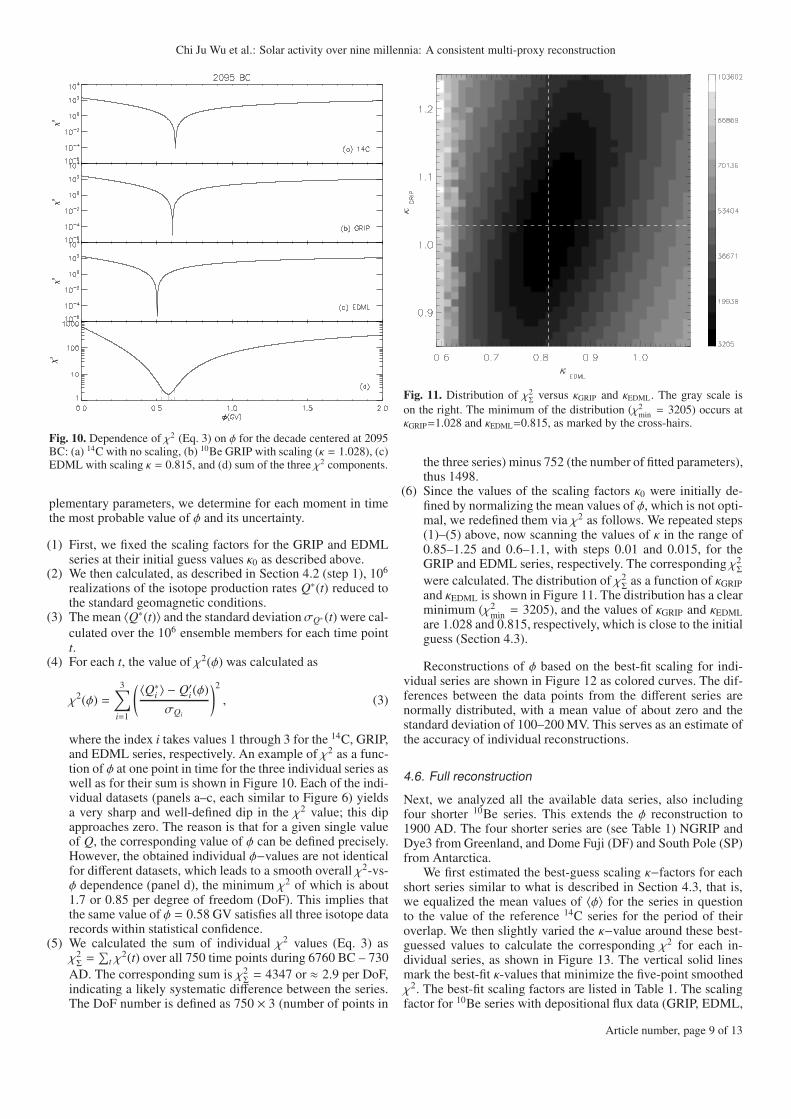
Fig. 11. Distribution of χ2Σ

versus κGRIP and κEDML. The gray scale is

on the right. The minimum of the distribution (χ2min= 3205) occurs at

κGRIP=1.028 and κEDML=0.815, as marked by the cross-hairs.

the three series) minus 752 (the number of fitted parameters),thus 1498.

(6) Since the values of the scaling factors κ0 were initially de-fined by normalizing the mean values of φ, which is not opti-mal, we redefined them via χ2 as follows. We repeated steps(1)–(5) above, now scanning the values of κ in the range of0.85–1.25 and 0.6–1.1, with steps 0.01 and 0.015, for theGRIP and EDML series, respectively. The corresponding χ2

Σ

were calculated. The distribution of χ2Σ

as a function of κGRIP

and κEDML is shown in Figure 11. The distribution has a clearminimum (χ2

min= 3205), and the values of κGRIP and κEDML

are 1.028 and 0.815, respectively, which is close to the initialguess (Section 4.3).

Reconstructions of φ based on the best-fit scaling for indi-vidual series are shown in Figure 12 as colored curves. The dif-ferences between the data points from the different series arenormally distributed, with a mean value of about zero and thestandard deviation of 100–200 MV. This serves as an estimate ofthe accuracy of individual reconstructions.

4.6. Full reconstruction

Next, we analyzed all the available data series, also includingfour shorter 10Be series. This extends the φ reconstruction to1900 AD. The four shorter series are (see Table 1) NGRIP andDye3 from Greenland, and Dome Fuji (DF) and South Pole (SP)from Antarctica.

We first estimated the best-guess scaling κ−factors for eachshort series similar to what is described in Section 4.3, that is,we equalized the mean values of 〈φ〉 for the series in questionto the value of the reference 14C series for the period of theiroverlap. We then slightly varied the κ−value around these best-guessed values to calculate the corresponding χ2 for each in-dividual series, as shown in Figure 13. The vertical solid linesmark the best-fit κ-values that minimize the five-point smoothedχ2. The best-fit scaling factors are listed in Table 1. The scalingfactor for 10Be series with depositional flux data (GRIP, EDML,



Fig. 12. Reconstruction of the modulation potential φ using only in-dividual cosmogenic isotope series (color curves as denoted in the leg-end) with the best-fit scaling (see Table 1) and the final composite series(thick black curve). The top and bottom panels depict the two halves ofthe entire interval. Only mean values are shown without uncertainties.

NGRIP, and Dome Fuji, see Table 1 and Figure 8) are close tounity (within 20%), which again implies that our model is quiterealistic. The 68% uncertainties are defined as corresponding to(

χ2min+ 1

)

.

Next, we performed the full reconstruction using the χ2

method described in Section 4.5, but now for all the series (seeFig. 12). The number of different series used to reconstruct in-dividual data points varied in time between two and five (seeFigure 1). The mean χ2 per DoF is 0.57, for 84% of data pointsχ2 < 1 per DoF, implying that the agreement between differentseries is good.

5. Reconstruction of the sunspot number

The modulation potential series alone are not very useful as asolar activity proxy since the modulation potential is a relativeindex whose absolute value is model dependent (Usoskin et al.2005; Herbst et al. 2010, 2017). Therefore, we converted themodulation potential, reconstructed in Section 4, into a moredefinitive index, the SN. This was done via the open solarmagnetic flux Fo, following an established procedure (e.g.,Usoskin et al. 2003; Solanki et al. 2004; Usoskin et al. 2016).Applying the updated SATIRE-M model (Vieira & Solanki2010; Vieira et al. 2011; Wu et al. 2018), we can write the re-lation (Usoskin et al. 2007, see the Appendix therein) betweenthe two indices as

SNi = 116 × φi + 33 × (φi+1 − φi) − 16, (4)

where the SN during the ith decade, SNi, is defined by the modu-lation potential (expressed in GV) during the contemporary andthe following decades. The negative offset term (-16) reflects thefact that zero SN during grand minima does not imply the ab-sence of GCR modulation, so that even when S N = 0, the valueof φ is about 0.14 GV (e.g., Owens et al. 2012). Since SNs can-not be negative, the SN was assigned zero values when the val-ues of φ dropped below the sunspot formation threshold. The

Fig. 13. Values of χ2 versus the scaling factors κ for four short 10Beseries, as marked in each panel. The five-point running mean curvesare shown in red. The locations of the best-fit κ−values are shown asstraight black lines.

uncertainties of the reconstructed S N values were defined byconverting the low- and upper-bound (68%) φ values (definedas described above) for each decade into SNs. The reconstructedSN series 3 is shown in Figure 14 along with its 68% confidenceinterval and is compared with the international SN series (SILSOISN version 2, Clette et al. 2014)4. Since we used SNs in their‘classical’ definition, the ISN v.2 data were scaled down by afactor 0.6 (as described in Clette et al. 2014).

The reconstructed solar activity varies at different timescalesfrom decades to millennia. In particular, a long period with rel-atively high activity occurred between roughly 4000 BC and1500 BC, and periods of lower activity occurred at ca. 5500BC and 1500 AD. The origin of this is unclear. For example,Usoskin et al. (2016) suggested, based on the fact that the GRIPand 14C series behave differently at this timescale, that it is aglobal climate effect rather than solar. As a result, they removedthis wave from the data in an ad hoc manner. However, as weshow here, it is more likely related to the undercorrection of theGRIP-based series and therefore may be related to solar activity,so that we retained it in the final dataset.

The new series is generally consistent with previous recon-structions (e.g., Usoskin et al. 2016), but it also has some newfeatures. In particular, it implies a lower activity during thesixth millennium BC. We note that a possible overestimation of

3 Available as a table in the supplementary ma-terials and at the MPS sun-climate web-pagehttp://www.mps.mpg.de/projects/sun-climate/data4 File SN_y_tot_V2.0.txt available at http://www.sidc.be/silso/ infos-nytot


http://www.mps.mpg.de/projects/sun-climate/data

http://www.sidc.be/silso/


Fig. 14. Reconstructed sunspot number along with its 68% confidence interval (gray shading). This series is available in the ancillary data. Thered line depicts the decadally resampled international sunspot number (version 2, scaled by 0.6) from Clette et al. (2014). The dashed line denotesthe level of SN=10.

the solar activity for this period has been suspected previously(Usoskin et al. 2007; Usoskin et al. 2016).

Although the overall level of solar activity may vary signif-icantly, the periods of grand minima may correspond to a spe-cial state of the solar dynamo (Schmitt et al. 1996; Küker et al.1999; Moss et al. 2008; Choudhuri & Karak 2012; Käpylä et al.2016) and thus are expected to provide roughly the same lowlevel of activity, corresponding to a virtual absence of sunspots.Thus, the level of the reconstructed activity during clearly dis-tinguishable grand minima may serve as a rough estimate of the‘stability’ of the reconstruction when we assume that activity al-ways drops to the same nearly zero level during each grand mini-mum (Sokoloff& Nesme-Ribes 1994; Usoskin et al. 2014). Theexpected level of solar activity during grand minima (SN→0) isindicated by the horizontal dashed line in Figure 14. The levelof the reconstructed grand minima (observed as sharp dips) isroughly consistent with SN→0 throughout almost the entire pe-riod, considering an uncertainty on the order of 10 in SN units.However, periods of 3500 BC – 2500 BC and before 5500 BCare characterized by a slightly higher SN level during the grandminima, suggesting a possible overestimation of activity duringthese times. Interestingly, no clear grand minima occurred dur-ing 2500 BC – 1000 BC, suggesting that it was a long period ofstable operation of the solar activity main mode.

The overall level of solar activity remained roughly con-stant, around 45–50, during most of the time, but appeared some-what lower (around 40) before 5000 BC, suggesting a possibleslow variability with a timescale of about 6–7 millennia (cf.,Usoskin et al. 2016). The reason for this is unknown, but it mightbe due to (1) climate influence, although this is expected to affect14C and 10Be isotopes differently; (2) solar activity, or (3) largesystematic uncertainty in the geomagnetic field reconstruction,which is poorly known before about 3000 BC.

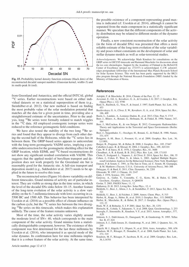
Figure 15 shows the kernel density estimation of the proba-bility density function (KDF) of the reconstructed decadal SNsfor the entire period (877 decades). The high peak of the distribu-tion with values around 40 is clearly visible; this corresponds to

moderate activity. A low-activity component with values below15 is clearly visible as well; this corresponds to a grand mini-mum. In addition, a bump is faintly visible at the high-activitytail (SN greater than 60, visible only as a small excess abovethe main Gaussian curve), suggesting a grand maximum compo-nent. In order to illustrate this, we applied a formal multi-peak(Gaussian) fit to the KDF, which is shown as the blue dottedcurves. The main peak is centered at decadal SN=42 (σ = 10)and represents the main component. Another peak can be foundas a small bump around SN=27 (σ = 6), but it is not sufficientlyseparated from the main component to justify calling it a sepa-rate component. The grand minimum component (Gaussian withσ = 6 centered at SN=12) is significantly separated from themain component (statistical significance p < 0.05). The separa-tion of the grand maximum component, while visible by eye asa deviation from the Gaussian shape at high values, is not statis-tically significant. The statistical separation of the special grandminimum component was first shown by Usoskin et al. (2014)for the last three millennia, while the result for the grand maxi-mum component was inconclusive.

Here we fully confirm this result over nine millennia, whichimplies that grand minimum and normal activity componentsform a robust feature of solar variability. This also suggests thatthe new reconstruction is more robust and less noisy than previ-ous reconstructions (e.g., Steinhilber et al. 2012; Usoskin et al.2016) and allows statistically identifying the grand minimumcomponent over 9000 years.

6. Conclusions

We have provided a new fully consistent multi-proxy reconstruc-tion of the solar activity over about nine millennia, based forthe first time on a Bayesian approach. We used all the availabledatasets of cosmogenic radioisotopes with sufficient length andquality in terrestrial archives and up-to-date models of isotopeproduction and transport or deposition as well as a recent archeo-magnetic model. We used six 10Be series of different lengths



0 10 20 30 40 50 60 70

1E-3

0.01

PD

F

Decadal SN

Fig. 15. Probability kernel density function estimate (black dots) of thereconstructed decadal sunspot numbers (Gaussian kernel, width=3) andits multi-peak fit (red).

from Greenland and Antarctica, and the official INTCAL global14C series. Earlier reconstructions were based on either indi-vidual datasets or on a statistical superposition of them (e.g.,Steinhilber et al. 2012). Our new method is based on findingthe most probable value of the solar modulation potential thatmatches all the data for a given point in time, providing also astraightforward estimate of the uncertainties. Prior to the anal-ysis, long 10Be series were formally redated to match wigglesin the 14C data. All employed cosmogenic isotope series werereduced to the reference geomagnetic field conditions.

We have also tested the stability of the two long 10Be se-ries and found that they appear to diverge from each other dur-ing the second half of the Holocene, while the 14C series lies inbetween them. The GRIP-based series appears to anticorrelatewith the long-term geomagnetic VADM series, implying a pos-sible undercorrection for the geomagnetic shielding effect for theGRIP location, while EDML and 14C-based reconstructions donot show any significant residual correlation with VADM. Thissuggests that the applied model of beryllium transport and de-position does not work properly for the Greenland site but isreasonably good for the Antarctic site. A full-size transport anddeposition model (e.g., Sukhodolov et al. 2017) needs to be ap-plied in the future to resolve this issue.

The reconstructed series (Figure 14) shows variability on dif-ferent timescales. Grand minima of activity are of particular in-terest. They are visible as strong dips in the time series, in whichthe level of the decadal SNs sinks below 10–15. Another featureof the long-term evolution of the solar activity is a slow vari-ability on the 6–7-millennia timescale with lows occurring in ca.5500 BC and 1500 AD. This behavior has been interpreted byUsoskin et al. (2016) as a possible effect of climate influence onthe carbon cycle, but the 14C series lies between the two diverg-ing 10Be series on this timescale, which makes this explanationunlikely. The cause of the feature remains unknown.

Most of the time, the solar activity varies slightly aroundthe moderate level of SN≈ 40, which corresponds to the maincomponent of the solar activity. Grand minima form a statisti-cally distinguishable component, however. The existence of thiscomponent was first determined for the last three millennia byUsoskin et al. (2014), who interpreted it as special mode of thesolar dynamo. Its confirmation here for nine millennia impliesthat it is a robust feature of the solar activity. At the same time,

the possible existence of a component representing grand max-ima is indicated (cf. Usoskin et al. 2014), although it cannot beseparated from the main component in a statistically significantmanner. We speculate that the different components of the activ-ity distribution may be related to different modes of the dynamooperation.

Finally, a new consistent reconstruction of the solar activity(in the form of decadal SNs) was presented that offers a morereliable estimate of the long-term evolution of the solar variabil-ity and poses robust constraints on the development of solar andstellar dynamo models as well as solar-terrestrial studies.

Acknowledgements. We acknowledge Mads Knudsen for consultations on theGRIP series in GICC05 timescale and Raimund Muscheler for discussions aboutthe ice core chronologies. Support by the Academy of Finland to the ReSoLVECenter of Excellence (project no. 272157) is acknowledged. C.J.W. acknowl-edges postgraduate fellowship of the International Max Planck Research Schoolfor Solar System Science. This work has been partly supported by the BK21plus program through the National Research Foundation (NRF) funded by theMinistry of Education of Korea.

References

Adolphi, F. & Muscheler, R. 2016, Climate of the Past, 12, 15Asvestari, E., Gil, A., Kovaltsov, G. A., & Usoskin, I. G. 2017, J. Geophys. Res.

(Space Phys.), 122, 9790Bard, E., Raisbeck, G., Yiou, F., & Jouzel, J. 1997, Earth Planet. Sci. Lett., 150,

453Bazilevskaya, G. A., Cliver, E. W., Kovaltsov, G. A., et al. 2014, Space Sci. Rev.,

186, 409Bazin, L., Landais, A., Lemieux-Dudon, B., et al. 2013, Clim. Past, 9, 1715Beer, J., Blinov, A., Bonani, G., Hofmann, H., & Finkel, R. 1990, Nature, 347,

164Beer, J., McCracken, K., & von Steiger, R. 2012, Cosmogenic Radionuclides:

Theory and Applications in the Terrestrial and Space Environments (Berlin:Springer)

Beer, J., Siegenthaler, U., Oeschger, H., Bonani, G., & Finkel, R. 1988, Nature,331, 675

Berggren, A.-M., Beer, J., Possnert, G., et al. 2009, Geophys. Res. Lett., 36,L11801,

Burger, R., Potgieter, M., & Heber, B. 2000, J. Geophys. Res., 105, 27447Caballero-Lopez, R. & Moraal, H. 2004, J. Geophys. Res., 109, A01101Cain, W. F. & Suess, H. E. 1976, J. Geophys. Res., 81, 3688Choudhuri, A. R. & Karak, B. B. 2012, Phys. Rev. Lett., 109, 171103Clette, F., Svalgaard, L., Vaquero, J., & Cliver, E. 2014, Space Sci. Rev., 186, 35Cohen, J., Cohen, P., West, S., & Aiken, L. 2003, Applied Multiple Regres-

sion/Correlation Analysis for the Behavioral Sciences (New York: Routledge)Damon, P. & Sonett, C. 1991, in The Sun in Time, ed. C. Sonett, M. Giampapa,

& M. Matthews (Tucson, U.S.A.: University of Arizona Press), 360–388Delaygue, G. & Bard, E. 2011, Clim. Dynamics, 36, 2201Ebisuzaki, W. 1997, J. Climate, 10, 2147Eddy, J. 1976, Science, 192, 1189Genevey, A., Gallet, Y., Constable, C. G., Korte, M., & Hulot, G. 2008,

Geochem., Geophys., Geosyst., 9, Q04038Goslar, T. 2003, PAGES News, 11, 12Hathaway, D. H. 2015, Living Rev. Solar Phys., 12, 4Heikkilä, U., Beer, J., Abreu, J. A., & Steinhilber, F. 2013, Space Sci. Rev., 176,

321Heikkilä, U., Beer, J., & Feichter, J. 2009, Atmos. Chem. Phys., 9, 515Herbst, K., Kopp, A., Heber, B., et al. 2010, J. Geophys. Res., 115, D00I20Herbst, K., Muscheler, R., & Heber, B. 2017, J. Geophys. Res. (Space Phys.),

122, 23Hoek, W. Z. & Bohncke, S. J. P. 2001, Quat. Sci. Rev., 20, 1251Horiuchi, K., Uchida, T., Sakamoto, Y., et al. 2008, Quat. Geochronology, 3, 253Inceoglu, F., Simoniello, R., Knudsen, V. F., et al. 2015, Astron. Astrophys., 577,

A20Johnsen, S. J., Dahl-Jensen, D., Dansgaard, W., & Gundestrup, N. 1995, Tellus

Ser. B, 47, 624Johnsen, S. J., Dahl-Jensen, D., Gundestrup, N., et al. 2001, J. Quatern. Sci., 16,

299Käpylä, M. J., Käpylä, P. J., Olspert, N., et al. 2016, Astro, Astrophys., 589, A56Knudsen, M. F., Riisager, P., Donadini, F., et al. 2008, Earth Planet. Sci. Lett.,

272, 319Knudsen, M. F., Riisager, P., Jacobsen, B. H., et al. 2009, Geophys. Res. Lett.,

36, L16701



Kovaltsov, G., Mishev, A., & Usoskin, I. 2012, Earth Planet. Sci. Lett., 337, 114Kovaltsov, G. & Usoskin, I. 2010, Earth Planet.Sci.Lett., 291, 182Küker, M., Arlt, R., & Rüdiger, G. 1999, Astron. Astrophys., 343, 977Licht, A., Hulot, G., Gallet, Y., & Thébault, E. 2013, Phys. Earth Planet. Inter.,

224, 38McCracken, K., McDonald, F., Beer, J., Raisbeck, G., & Yiou, F. 2004, J. Geo-

phys. Res., 109, 12103McCracken, K. G. & Beer, J. 2015, Solar Phys., 290, 3051Mekhaldi, F., Muscheler, R., Adolphi, F., et al. 2015, Nature Comm., 6, 8611Miyake, F., Jull, A. J. T., Panyushkina, I. P., et al. 2017, Proc. Nat. Acad. Sci.,

114, 881Miyake, F., Masuda, K., & Nakamura, T. 2013, Nature Comm., 4, 1748Miyake, F., Nagaya, K., Masuda, K., & Nakamura, T. 2012, Nature, 486, 240Moss, D., Sokoloff, D., Usoskin, I., & Tutubalin, V. 2008, Solar Phys., 250, 221Muscheler, R., Adolphi, F., & Knudsen, M. F. 2014, Quat. Sci. Rev., 106, 81Muscheler, R., Beer, J., Wagner, G., et al. 2004, Earth Planet. Sci. Lett., 219, 325Muscheler, R., Joos, F., Beer, J., et al. 2007, Quater. Sci. Rev., 26, 82Nilsson, A., Holme, R., Korte, M., Suttie, N., & Hill, M. 2014, Geophys. J. Int.,

198, 229Owens, M. J., Usoskin, I., & Lockwood, M. 2012, Geophys. Res. Lett., 39,

L19102Pavlov, A. K., Blinov, A. V., Frolov, D. A., et al. 2017, Journal of Atmospheric

and Solar-Terrestrial Physics, 164, 308Pavón-Carrasco, F. J., Osete, M. L., Torta, J. M., & De Santis, A. 2014, Earth

Planet. Sci. Lett., 388, 98Poluianov, S. V., Kovaltsov, G. A., Mishev, A. L., & Usoskin, I. G. 2016, J.

Geophys. Res. (Atm.), 121, 8125Raisbeck, G., Yiou, F., Jouzel, J., & Petit, J. 1990, Royal Soc. London Philos.

Trans. Ser. A, 330, 463Rasmussen, S. O., Bigler, M., Blockley, S. P., et al. 2014, Quat. Sci. Rev., 106,

14Reimer, P. J., Baillie, M. G. L., Bard, E., et al. 2009, Radiocarbon, 51, 1111Ribes, J. & Nesme-Ribes, E. 1993, Astron. Astrophys., 276, 549Roth, R. & Joos, F. 2013, Clim. Past, 9, 1879Schmitt, D., Schüssler, M., & Ferriz-Mas, A. 1996, Astron. Astrophys., 311, L1Seierstad, I. K., Abbott, P. M., Bigler, M., et al. 2014, Quat. Sci. Rev., 106, 29Sigl, M., Winstrup, M., McConnell, J. R., et al. 2015, Nature, 523, 543Sokoloff, D. & Nesme-Ribes, E. 1994, Astron. Astrophys., 288, 293Solanki, S. K., Usoskin, I. G., Kromer, B., Schüssler, M., & Beer, J. 2004, Nature,

431, 1084Steinhilber, F., Abreu, J., Beer, J., et al. 2012, Proc. Nat. Acad. Sci. USA, 109,

5967Stuiver, M. 1961, J. Geophys. Res., 66, 273Stuiver, M. & Braziunas, T. 1989, Nature, 338, 405Stuiver, M. & Quay, P. 1980, Science, 207, 11Sukhodolov, T., Usoskin, I., Rozanov, E., et al. 2017, Sci. Rep., 7, 45257Usoskin, I. G. 2017, Living Rev. Solar Phys., 14, 3Usoskin, I. G., Alanko-Huotari, K., Kovaltsov, G. A., & Mursula, K. 2005, J.

Geophys. Res., 110, A12108Usoskin, I. G., Arlt, R., Asvestari, E., et al. 2015, Astron. Astrophys., 581, A95Usoskin, I. G., Gallet, Y., Lopes, F., Kovaltsov, G. A., & Hulot, G. 2016, Astron.

Astrophys., 587, A150Usoskin, I. G., Horiuchi, K., Solanki, S., Kovaltsov, G. A., & Bard, E. 2009, J.

Geophys. Res., 114, A03112Usoskin, I. G., Hulot, G., Gallet, Y., et al. 2014, Astron. Astrophys., 562, L10Usoskin, I. G. & Kovaltsov, G. A. 2012, Astrophys. J., 757, 92Usoskin, I. G., Kromer, B., Ludlow, F., et al. 2013, Astron. Astrophys., 552, L3Usoskin, I. G., Solanki, S. K., & Kovaltsov, G. A. 2007, Astron. Astrophys., 471,

301Usoskin, I. G., Solanki, S. K., Schüssler, M., Mursula, K., & Alanko, K. 2003,

Phys. Rev. Lett., 91, 211101Vaquero, J. M., Kovaltsov, G. A., Usoskin, I. G., Carrasco, V. M. S., & Gallego,

M. C. 2015, Astron. Astrophys., 577, A71Veres, D., Bazin, L., Landais, A., et al. 2013, Clim. Past, 9, 1733Vieira, L. E. A. & Solanki, S. K. 2010, Astron. Astrophys., 509, A100Vieira, L. E. A., Solanki, S. K., Krivova, N. A., & Usoskin, I. 2011, Astron.

Astrophys., 531, A6Vinther, B. M., Clausen, H. B., Johnsen, S. J., et al. 2006, J. Geophys. Res.

(Atm.), 111, D13102Vonmoos, M., Beer, J., & Muscheler, R. 2006, J. Geophys. Res., 111, A10105Wu, C.-J., Krivova, N. A., Solanki, S. K., & Usoskin, I. G. 2018, Astron. Astro-

phys., (submitted)Yiou, F., Raisbeck, G., Baumgartner, S., et al. 1997, J. Geophys. Res., 102, 26783


Documents

Solar activity over nine millennia: A consistent multi ... · studies were based on individual, sometimes statistically averaged, proxy datasets. Here we aim to provide a new consistent