SOIL SALINITY MAPPING USING MULTITEMPORAL LANDSAT … · SOIL SALINITY MAPPING USING MULTITEMPORAL LANDSAT DATA. ... [email protected]. ... the most severe problems among the

SOIL SALINITY MAPPING USING MULTITEMPORAL LANDSAT DATA

A. Azabdaftari a, F. Sunarb

aIstanbul Technical University, Informatics Inistitue, Communication Systems Dept.,34469, Maslak Istanbul, Turkey

[email protected] bIstanbul Technical University, Civil Engineering Faculty, Geomatics Engineering Dept., 34469, Maslak Istanbul, Turkey

[email protected]

Commission VII, WG VII/1

KEY WORDS: Remote sensing, Soil salinity, Landsat data, Salinity index, Vegetation index

ABSTRACT:

Soil salinity is one of the most important problems affecting many areas of the world. Saline soils present in agricultural areas reduce the annual yields of most crops. This research deals with the soil salinity mapping of Seyhan plate of Adana district in Turkey from the years 2009 to 2010, using remote sensing technology. In the analysis, multitemporal data acquired from LANDSAT 7-

ETM+ satellite in four different dates (19 April 2009, 12 October 2009, 21 March 2010, 31 October 2010) are used. As a first step, preprocessing of Landsat images is applied. Several salinity indices such as NDSI (Normalized Difference Salinity Index), BI (Brightness Index) and SI (Salinity Index) are used besides some vegetation indices such as NDVI (Normalized Difference Vegetation Index), RVI (Ratio Vegetation Index), SAVI (Soil Adjusted Vegetation Index) and EVI (Enhamced Vegetation Index) for the soil salinity mapping of the study area. The field’s electrical conductivity (EC) measurements done in 2009 and 2010, are used as a ground truth data for the correlation analysis with the original band values and different index image bands values. In the correlation analysis, two regression models, the simple linear regression (SLR) and multiple linear regression (MLR) are considered. According to the highest correlation obtained, the 21st March, 2010 dataset is chosen for production of the soil salinity map in the area. Finally, the efficiency of the remote sensing technology in the soil salinity mapping is outlined.

1. INTRODUCTION

Soil salinity is one of the widespread environmental hazards

all around the world, especially in arid and semiarid

regions. Soil salinization that mainly occurs due to

irrigation and other intensified agricultural activities, is one of

the most severe problems among the many forms of soil

degradation (Akramkhanov, 2011). The development of saline

soils is a dynamic phenomenon, which needs to be monitored

regularly in order to secure up to date knowledge of their

extent, degree of severity, spatial distribution, nature and

magnitude. For monitoring dynamic processes, like

salinization, remotely sensed data has great potential; it uses

aerial photography, thermal infrared or multispectral data

acquired from platforms such as Landsat satellite (Allbed and

Kumar, 2013). Previously, soil salinity has been measured

by collecting soil samples in the region of interest, and then

the samples were analyzed in laboratory in order to

determine the amount of electric conductivity in the soil but

this method was time and cost consuming. However, remote

sensing data offer more efficiently and economically rapid

means and techniques for monitoring and mapping soil

salinity. There are many satellites and sensors, which are

useful in detecting and monitoring the saline soil.

Multispectral data such as LANDSAT, SPOT, IKONOS, EO-

1, IRS, and Terra-ASTER with the resolution can be ranged

from medium to high as well as hyperspectral sensors.

The sensors scan only the soil surface, while the entire soil

profile is involved and should be considered. This limitation

highlights the necessity of using other data and techniques, in

combination with remote sensing (Farifteh, 2006). The main

objectives of this study are: (i) to understand the spectral

reflectance characteristics of saline soil in Seyhan plate, (ii) to

explore the potential of Landsat imagery to detect and map the

soil salinity over the study area, (iii) to analyse the correlation

between field measurements and Landsat imagery, and (iv) to

produce the soil salinity map according to high, moderate and

low saline content.

2. STUDY AREA

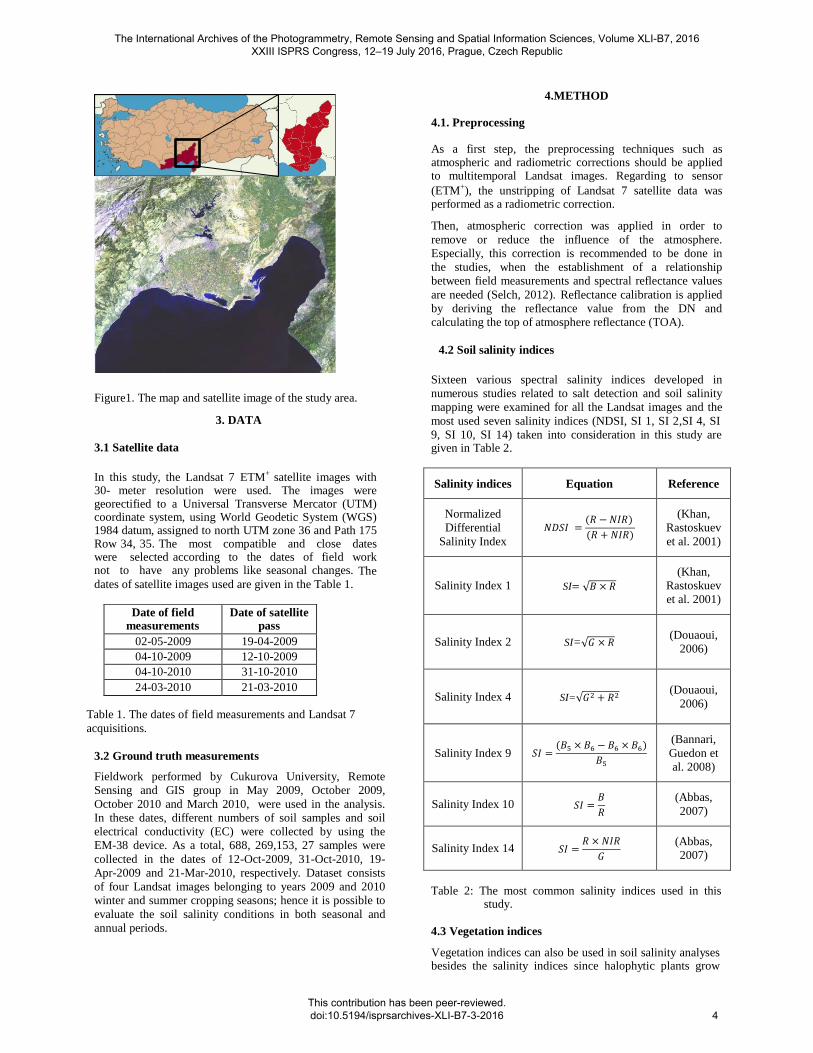
Çukurova is a district in south central of Turkey covering the provinces of Adana and Mersin (Figure 1). It is located in the coordinates of 37°02′52″ North latitudes and 35°17′54″ East longitudes. The total area of the Çukurova is about 38,000 km2, Turkey’s biggest delta plain with a large stretch of flat and fertile land, which is among the most agriculturally productive areas of the world. The climate is relatively mild and humid in the winter months and the alluvial soils make the area highly suitable for agriculture. Akarsu irrigation basin and Seyhan plate are located in Çukurova plain.

The International Archives of the Photogrammetry, Remote Sensing and Spatial Information Sciences, Volume XLI-B7, 2016 XXIII ISPRS Congress, 12–19 July 2016, Prague, Czech Republic

This contribution has been peer-reviewed. doi:10.5194/isprsarchives-XLI-B7-3-2016

3

mailto:[email protected]




http://en.wikipedia.org/wiki/Turkey

http://en.wikipedia.org/wiki/Adana_Province

4.METHOD

4.1. Preprocessing

As a first step, the preprocessing techniques such as atmospheric and radiometric corrections should be applied to multitemporal Landsat images. Regarding to sensor

(ETM+), the unstripping of Landsat 7 satellite data was performed as a radiometric correction.

Then, atmospheric correction was applied in order to

remove or reduce the influence of the atmosphere.

Especially, this correction is recommended to be done in

the studies, when the establishment of a relationship

between field measurements and spectral reflectance values

are needed (Selch, 2012). Reflectance calibration is applied

by deriving the reflectance value from the DN and

calculating the top of atmosphere reflectance (TOA).

Figure1. The map and satellite image of the study area.

3. DATA

3.1 Satellite data

In this study, the Landsat 7 ETM+ satellite images with 30- meter resolution were used. The images were georectified to a Universal Transverse Mercator (UTM) coordinate system, using World Geodetic System (WGS) 1984 datum, assigned to north UTM zone 36 and Path 175 Row 34, 35. The most compatible and close dates were selected according to the dates of field work not to have any problems like seasonal changes. The dates of satellite images used are given in the Table 1.

Table 1. The dates of field measurements and Landsat 7

acquisitions.

3.2 Ground truth measurements

Fieldwork performed by Cukurova University, Remote

Sensing and GIS group in May 2009, October 2009,

October 2010 and March 2010, were used in the analysis.

In these dates, different numbers of soil samples and soil

electrical conductivity (EC) were collected by using the

EM-38 device. As a total, 688, 269,153, 27 samples were

collected in the dates of 12-Oct-2009, 31-Oct-2010, 19-

Apr-2009 and 21-Mar-2010, respectively. Dataset consists

of four Landsat images belonging to years 2009 and 2010

winter and summer cropping seasons; hence it is possible to

evaluate the soil salinity conditions in both seasonal and

annual periods.

4.2 Soil salinity indices

Sixteen various spectral salinity indices developed in

numerous studies related to salt detection and soil salinity

mapping were examined for all the Landsat images and the

most used seven salinity indices (NDSI, SI 1, SI 2,SI 4, SI

9, SI 10, SI 14) taken into consideration in this study are given in Table 2.

Salinity indices Equation Reference

Normalized

Differential

Salinity Index

(Khan,

Rastoskuev

et al. 2001)

Salinity Index 1 SI √

(Khan,

Rastoskuev

et al. 2001)

Salinity Index 2 SI=√ (Douaoui,

2006)

Salinity Index 4 SI=√ (Douaoui,

2006)

Salinity Index 9

(Bannari,

Guedon et

al. 2008)

Salinity Index 10

(Abbas,

2007)

Salinity Index 14

(Abbas,

2007)

Table 2: The most common salinity indices used in this

study.

4.3 Vegetation indices

Vegetation indices can also be used in soil salinity analyses besides the salinity indices since halophytic plants grow

Date of field measurements

Date of satellite pass

02-05-2009 19-04-2009

04-10-2009 12-10-2009

04-10-2010 31-10-2010

24-03-2010 21-03-2010



4

naturally in saline soils, and can be adapted to high soil

salinity. Therefore, vegetation has been used as an indirect

indicator to predict and map soil salinity. Four different

vegetation indices were applied and among them two most

common vegetation indices (Table 3) showing better

correlation were taken into consideration.

Vegetation

Indices Equation

Normalized

Differential

Vegetation Index

Soil Adjusted

Vegetation Index

Table 3. The vegetation indices used in this study.

4.5 Correlation

In this step, the correlation between electrical conductivity

of the collected field samples and band values of satellite

images is carried out to find the relationship between these

variables and assess their efficiency in predicting soil

salinity using Simple Linear Regression (SLR) and

Multiple Linear Regression (MLR) techniques. Regression

modeling techniques are widely used for predicting a

variable’s spatial distribution (Palialexis, 2011).

4.5.1 Simple linear regression

The SLR model was applied by using a single band values

for predicting soil salinity. To compute the single band

correlation, the digital values corresponding to each sample

was extracted for each band in the Landsat images and this

has been carried out for all data set (2009 - 2010) to

develop the relationship with in-situ electrical conductivity

measurements done in both vertical and horizontal

orientations. The same process was applied to the

radiometrically corrected TOA value of sample points in

order to evaluate the correlation with salinity

measurements. The correlation of in-situ EC values with

both DN and TOA values was assessed.

The univariate analysis showed that all bands are not

statistically significant predictors of salinity, and not any

specific differences were found between the correlation of

EC value with either DN or TOA in all satellite image

dataset. As a second step, twenty indices including sixteen

salinity indices and four vegetation indices were used as a

part of the correlation analysis. These indices were chosen

with regard to the relevant literature based on their

efficiencies in the soil salinity mapping. Hence, the

correlation analyses between each indices with EC value in

each date was performed using linear regression method to

investigate the strongest correlation with the sampled soil

salinity values. Similar to correlation of DN and EC values,

the correlation of different indices with the in-situ soil

salinity measurements was not sufficient

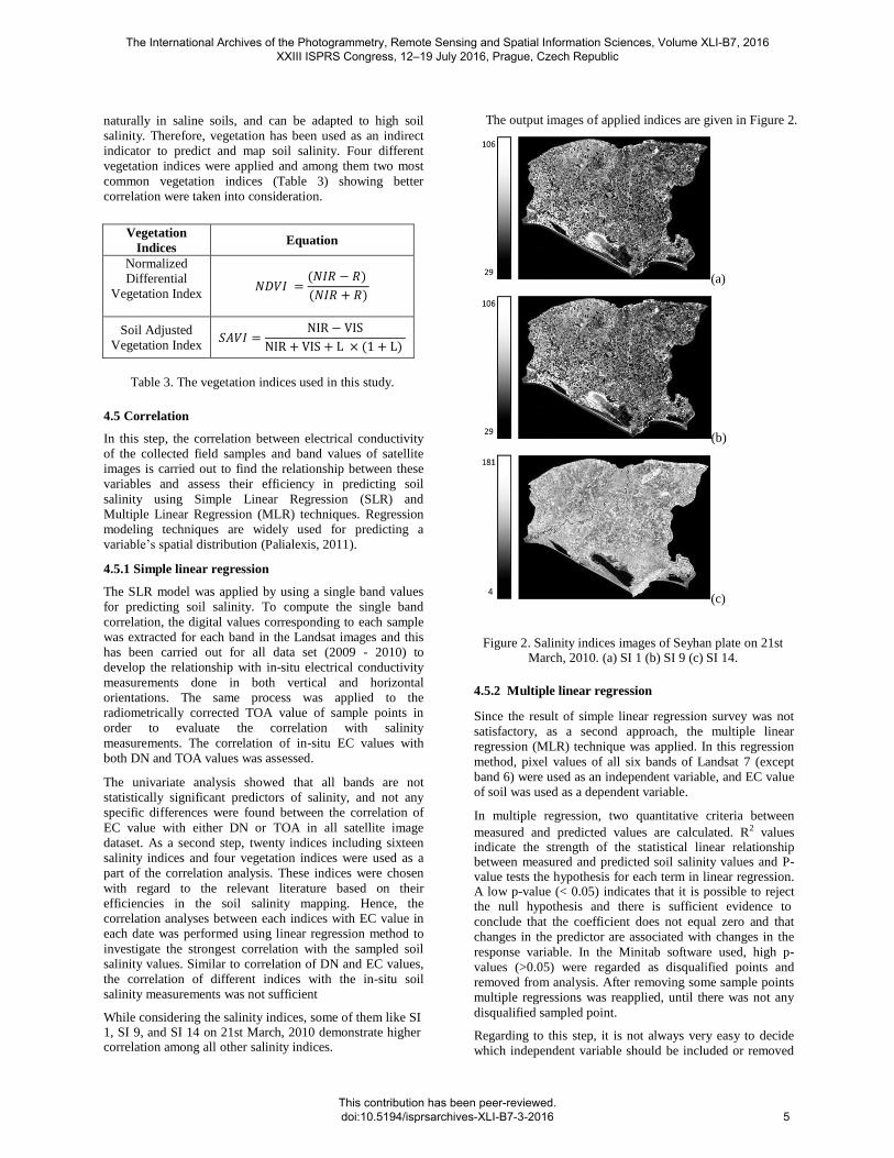
While considering the salinity indices, some of them like SI 1, SI 9, and SI 14 on 21st March, 2010 demonstrate higher correlation among all other salinity indices.

The output images of applied indices are given in Figure 2.

(a)

(b)

(c)

Figure 2. Salinity indices images of Seyhan plate on 21st March, 2010. (a) SI 1 (b) SI 9 (c) SI 14.

4.5.2 Multiple linear regression

Since the result of simple linear regression survey was not

satisfactory, as a second approach, the multiple linear

regression (MLR) technique was applied. In this regression

method, pixel values of all six bands of Landsat 7 (except

band 6) were used as an independent variable, and EC value

of soil was used as a dependent variable.

In multiple regression, two quantitative criteria between

measured and predicted values are calculated. R2 values indicate the strength of the statistical linear relationship between measured and predicted soil salinity values and P- value tests the hypothesis for each term in linear regression. A low p-value (< 0.05) indicates that it is possible to reject the null hypothesis and there is sufficient evidence to

conclude that the coefficient does not equal zero and that

changes in the predictor are associated with changes in the

response variable. In the Minitab software used, high p-

values (>0.05) were regarded as disqualified points and

removed from analysis. After removing some sample points

multiple regressions was reapplied, until there was not any

disqualified sampled point.

Regarding to this step, it is not always very easy to decide

which independent variable should be included or removed



5

http://blog.minitab.com/blog/adventures-in-statistics/how-to-correctly-interpret-p-values

from the regression, since the use of too much variables

may lead to poor prediction. Therefore, stepwise regression

was used as a solution to overcome this issue.

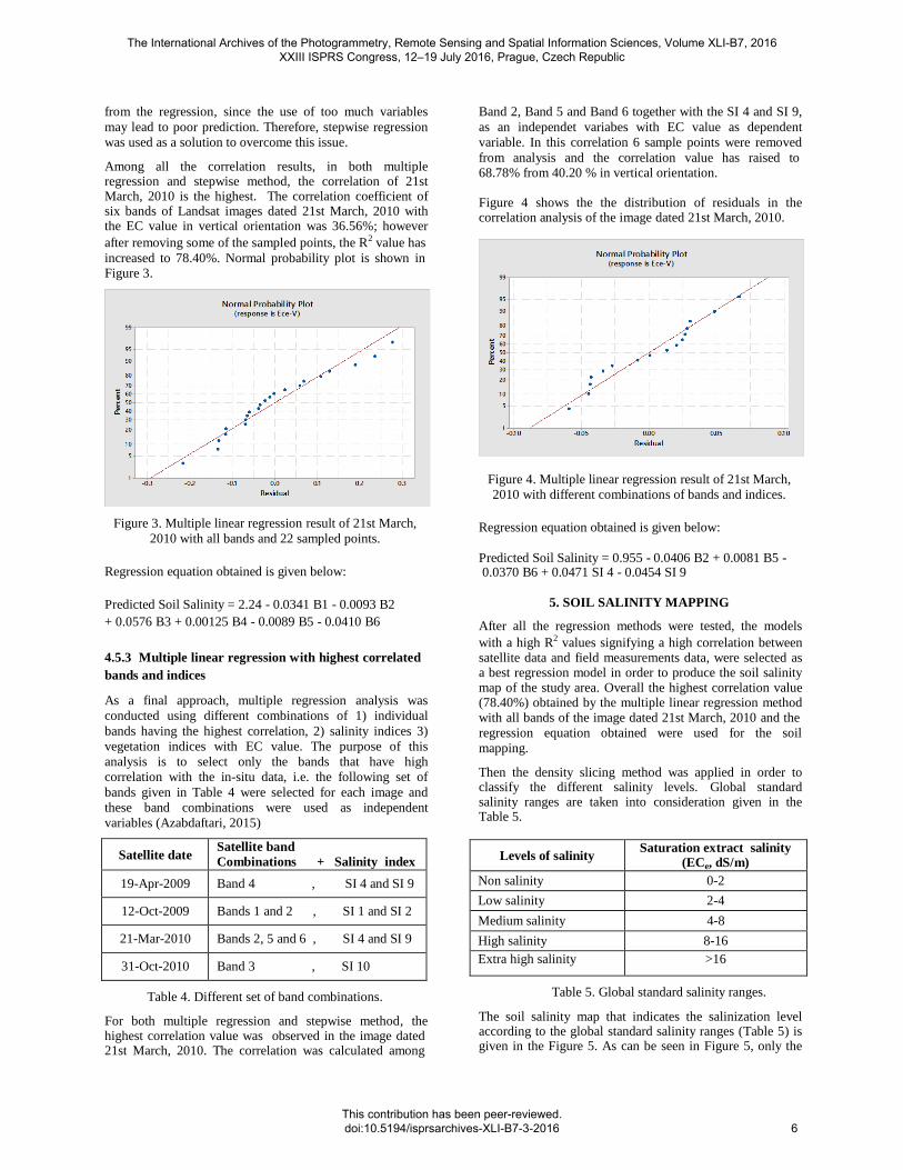
Among all the correlation results, in both multiple regression and stepwise method, the correlation of 21st March, 2010 is the highest. The correlation coefficient of six bands of Landsat images dated 21st March, 2010 with the EC value in vertical orientation was 36.56%; however

after removing some of the sampled points, the R2 value has

increased to 78.40%. Normal probability plot is shown in Figure 3.

Figure 3. Multiple linear regression result of 21st March,

2010 with all bands and 22 sampled points.

Regression equation obtained is given below:

Predicted Soil Salinity = 2.24 - 0.0341 B1 - 0.0093 B2

+ 0.0576 B3 + 0.00125 B4 - 0.0089 B5 - 0.0410 B6

4.5.3 Multiple linear regression with highest correlated

bands and indices

As a final approach, multiple regression analysis was

conducted using different combinations of 1) individual

bands having the highest correlation, 2) salinity indices 3)

vegetation indices with EC value. The purpose of this

analysis is to select only the bands that have high

correlation with the in-situ data, i.e. the following set of

bands given in Table 4 were selected for each image and

these band combinations were used as independent

variables (Azabdaftari, 2015)

Satellite date Satellite band Combinations + Salinity index

19-Apr-2009 Band 4 , SI 4 and SI 9

12-Oct-2009 Bands 1 and 2 , SI 1 and SI 2

21-Mar-2010 Bands 2, 5 and 6 , SI 4 and SI 9

31-Oct-2010 Band 3 , SI 10

Table 4. Different set of band combinations.

For both multiple regression and stepwise method, the highest correlation value was observed in the image dated 21st March, 2010. The correlation was calculated among

Band 2, Band 5 and Band 6 together with the SI 4 and SI 9,

as an independet variabes with EC value as dependent

variable. In this correlation 6 sample points were removed

from analysis and the correlation value has raised to 68.78% from 40.20 % in vertical orientation. Figure 4 shows the the distribution of residuals in the correlation analysis of the image dated 21st March, 2010.

Figure 4. Multiple linear regression result of 21st March,

2010 with different combinations of bands and indices.

Regression equation obtained is given below:

Predicted Soil Salinity = 0.955 - 0.0406 B2 + 0.0081 B5 - 0.0370 B6 + 0.0471 SI 4 - 0.0454 SI 9

5. SOIL SALINITY MAPPING

After all the regression methods were tested, the models

with a high R2 values signifying a high correlation between satellite data and field measurements data, were selected as a best regression model in order to produce the soil salinity map of the study area. Overall the highest correlation value (78.40%) obtained by the multiple linear regression method with all bands of the image dated 21st March, 2010 and the

regression equation obtained were used for the soil

mapping.

Then the density slicing method was applied in order to classify the different salinity levels. Global standard salinity ranges are taken into consideration given in the Table 5.

Levels of salinity Saturation extract salinity

(ECe, dS/m)

Non salinity 0-2

Low salinity 2-4

Medium salinity 4-8

High salinity 8-16

Extra high salinity >16

Table 5. Global standard salinity ranges.

The soil salinity map that indicates the salinization level according to the global standard salinity ranges (Table 5) is given in the Figure 5. As can be seen in Figure 5, only the



6

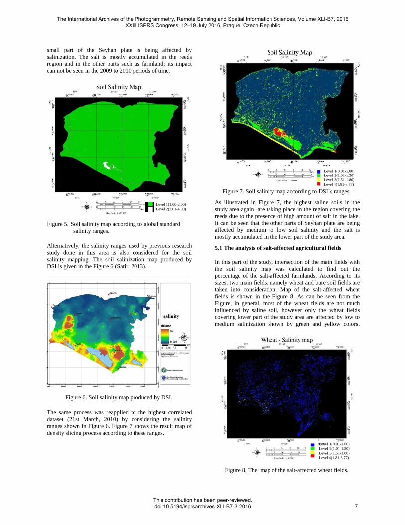
small part of the Seyhan plate is being affected by

salinization. The salt is mostly accumulated in the reeds

region and in the other parts such as farmland; its impact

can not be seen in the 2009 to 2010 periods of time.

Level 1(0.01-1.00)

Level 2(1.01-1.50)

Level 3(1.51-1.80)

Level 4(1.81-3.77)

Level 1(1.00-2.00)

Level 2(2.01-4.00)

Figure 5. Soil salinity map according to global standard

salinity ranges.

Alternatively, the salinity ranges used by previous research

study done in this area is also considered for the soil

salinity mapping. The soil salinization map produced by

DSI is given in the Figure 6 (Satir, 2013).

Figure 6. Soil salinity map produced by DSI.

The same process was reapplied to the highest correlated

dataset (21st March, 2010) by considering the salinity

ranges shown in Figure 6. Figure 7 shows the result map of

density slicing process according to these ranges.

Figure 7. Soil salinity map according to DSI’s ranges.

As illustrated in Figure 7, the highest saline soils in the

study area again are taking place in the region covering the

reeds due to the presence of high amount of salt in the lake.

It can be seen that the other parts of Seyhan plate are being

affected by medium to low soil salinity and the salt is

mostly accumulated in the lower part of the study area.

5.1 The analysis of salt-affected agricultural fields

In this part of the study, intersection of the main fields with

the soil salinity map was calculated to find out the

percentage of the salt-affected farmlands. According to its

sizes, two main fields, namely wheat and bare soil fields are

taken into consideration. Map of the salt-affected wheat

fields is shown in the Figure 8. As can be seen from the

Figure, in general, most of the wheat fields are not much

influenced by saline soil, however only the wheat fields

covering lower part of the study area are affected by low to

medium salinization shown by green and yellow colors.

Level 1(0.01-1.00)

Level 2(1.01-1.50)

Level 3(1.51-1.80)

Level 4(1.81-3.77)

Figure 8. The map of the salt-affected wheat fields.



7

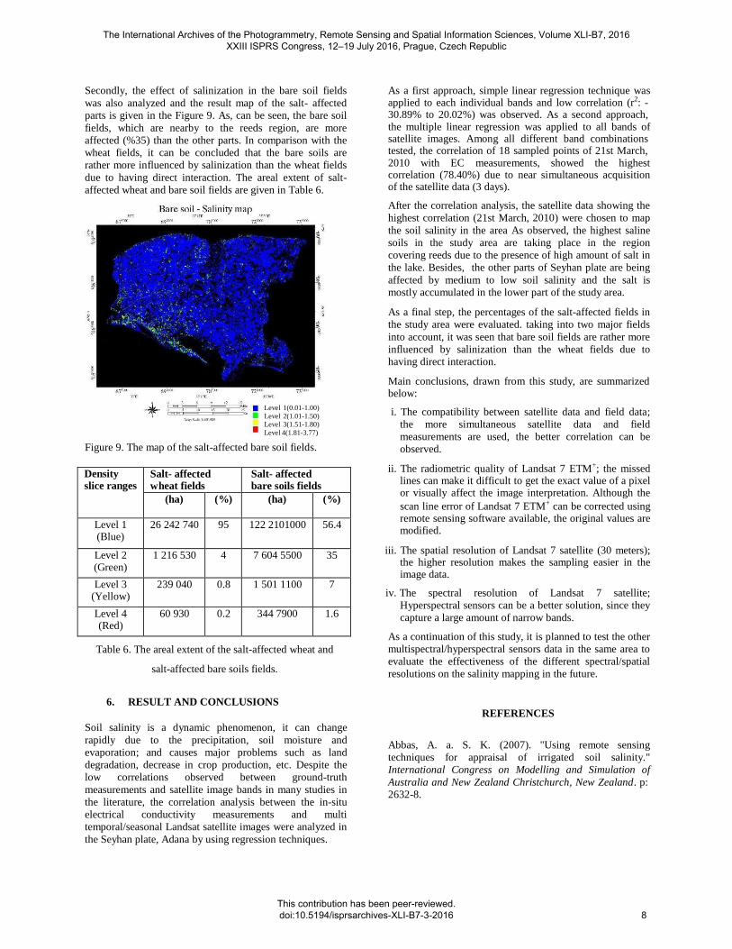
Secondly, the effect of salinization in the bare soil fields

was also analyzed and the result map of the salt- affected

parts is given in the Figure 9. As, can be seen, the bare soil

fields, which are nearby to the reeds region, are more

affected (%35) than the other parts. In comparison with the

wheat fields, it can be concluded that the bare soils are

rather more influenced by salinization than the wheat fields

due to having direct interaction. The areal extent of salt-

affected wheat and bare soil fields are given in Table 6.

Level 1(0.01-1.00)

Level 2(1.01-1.50)

Level 3(1.51-1.80)

Level 4(1.81-3.77)

Figure 9. The map of the salt-affected bare soil fields.

Density slice ranges

Salt- affected wheat fields

Salt- affected bare soils fields

(ha) (%) (ha) (%)

Level 1 (Blue)

26 242 740 95 122 2101000 56.4

Level 2 (Green)

1 216 530 4 7 604 5500 35

Level 3 (Yellow)

239 040 0.8 1 501 1100 7

Level 4 (Red)

60 930 0.2 344 7900 1.6

Table 6. The areal extent of the salt-affected wheat and

salt-affected bare soils fields.

6. RESULT AND CONCLUSIONS

Soil salinity is a dynamic phenomenon, it can change

rapidly due to the precipitation, soil moisture and

evaporation; and causes major problems such as land

degradation, decrease in crop production, etc. Despite the

low correlations observed between ground-truth

measurements and satellite image bands in many studies in

the literature, the correlation analysis between the in-situ

electrical conductivity measurements and multi

temporal/seasonal Landsat satellite images were analyzed in

the Seyhan plate, Adana by using regression techniques.

As a first approach, simple linear regression technique was applied to each individual bands and low correlation (r2: - 30.89% to 20.02%) was observed. As a second approach, the multiple linear regression was applied to all bands of satellite images. Among all different band combinations tested, the correlation of 18 sampled points of 21st March, 2010 with EC measurements, showed the highest correlation (78.40%) due to near simultaneous acquisition of the satellite data (3 days).

After the correlation analysis, the satellite data showing the

highest correlation (21st March, 2010) were chosen to map

the soil salinity in the area As observed, the highest saline

soils in the study area are taking place in the region

covering reeds due to the presence of high amount of salt in

the lake. Besides, the other parts of Seyhan plate are being

affected by medium to low soil salinity and the salt is

mostly accumulated in the lower part of the study area.

As a final step, the percentages of the salt-affected fields in

the study area were evaluated. taking into two major fields

into account, it was seen that bare soil fields are rather more

influenced by salinization than the wheat fields due to

having direct interaction.

Main conclusions, drawn from this study, are summarized below:

i. The compatibility between satellite data and field data;

the more simultaneous satellite data and field

measurements are used, the better correlation can be

observed.

ii. The radiometric quality of Landsat 7 ETM+; the missed lines can make it difficult to get the exact value of a pixel or visually affect the image interpretation. Although the

scan line error of Landsat 7 ETM+ can be corrected using remote sensing software available, the original values are modified.

iii. The spatial resolution of Landsat 7 satellite (30 meters); the higher resolution makes the sampling easier in the image data.

iv. The spectral resolution of Landsat 7 satellite;

Hyperspectral sensors can be a better solution, since they

capture a large amount of narrow bands.

As a continuation of this study, it is planned to test the other

multispectral/hyperspectral sensors data in the same area to

evaluate the effectiveness of the different spectral/spatial

resolutions on the salinity mapping in the future.

REFERENCES

Abbas, A. a. S. K. (2007). "Using remote sensing

techniques for appraisal of irrigated soil salinity."

International Congress on Modelling and Simulation of

Australia and New Zealand Christchurch, New Zealand. p: 2632-8.



8

Akramkhanov, A., C. Martius, S. J. Park and J. M. H.

Hendrickx (2011). "Environmental factors of spatial

distribution of soil salinity on flat irrigated terrain."

Geoderma, 163(1-2): 55-62.

Allbed, A. and L. Kumar (2013). "Soil salinity mapping and monitoring in arid and semi-arid regions using remote sensing technology: A review." Advances in Remote Sensing 2013 (2): 373-385.

Azabdaftari, A. (2015). "Soil salinity mapping by

integrating remote sensing data with ground measurements;

A case study in lower seyhan plate, Adana, Turkey."

Informatic Inistitute, Istanbul Technical University.

Bannari, A., A. Guedon, A. El‐Harti, F. Cherkaoui and A.

El‐Ghmari (2008). "Characterization of Slightly and

Moderately Saline and Sodic Soils in Irrigated Agricultural

Land using Simulated Data of Advanced Land Imaging

(EO‐1) Sensor." Communications in soil science and plant

analysis 39(19-20): 2795-2811.

Douaoui, A. E. K., H. Nicolas and C. Walter (2006).

"Detecting salinity hazards within a semiarid context by

means of combining soil and remote-sensing data."

Geoderma 134(1): 217-230.

Farifteh, J., A. Farshad and R. George (2006). "Assessing

salt-affected soils using remote sensing, solute modelling,

and geophysics." Geoderma 130(3): 191-206.

Khan, N. M., V. V. Rastoskuev, E. V. Shalina and Y. Sato (2001). "Mapping salt-affected soils using remote sensing indicators-a simple approach with the use of GIS IDRISI." 22nd Asian Conference on Remote Sensing, 5(9).

Palialexis, A., S. Georgakarakos, I. Karakassis, K. Lika and

V. Valavanis (2011). "Fish distribution predictions from

different points of view: comparing associative neural

networks, geostatistics and regression models."

Hydrobiologia 670(1): 165-188.

Satır, O. (2013). "Aşağı Seyhan ovası'nda uzaktan algılama

ve coğrafi bilgi sistemleri yardımıyla tarımsal alan kullanım

uygunluğunun belirlenmesi." Graduate School of Science,

Engineering and Technology, Çukurova University.

Selch, D. (2012). Comparing salinity models in Whitewater Bay using remote sensing, Florida Atlantic University.



9

Documents

SOIL SALINITY MAPPING USING MULTITEMPORAL LANDSAT … · SOIL SALINITY MAPPING USING MULTITEMPORAL LANDSAT DATA. ... [email protected]. ... the most severe problems among the