Soil Physics Simulation of Overwinter Soil Water and Soil …. zizhon… · · 2017-08-02viving through the cold winter (Lauriault et al., 2002; Lauriault et al., 2005). ... and

Soil Science Society of America Journal

Soil Sci. Soc. Am. J. 76:1548–1563 doi:10.2136/sssaj2011.0434 Received 16 Dec. 2011. *Corresponding author ([email protected]). © Soil Science Society of America, 5585 Guilford Rd., Madison WI 53711 USA All rights reserved. No part of this periodical may be reproduced or transmitted in any form or by any means, electronic or mechanical, including photocopying, recording, or any information storage and retrieval system, without permission in writing from the publisher. Permission for printing and for reprinting the material contained herein has been obtained by the publisher.

Simulation of Overwinter Soil Water and Soil Temperature with SHAW and RZ-SHAW

Soil Physics

Soil physical, chemical, and biological processes in agricultural systems and other terrestrial ecosystems depend greatly on soil water and temperature con-ditions. The latter conditions are especially critical to overwintering crops sur-

viving through the cold winter (Lauriault et al., 2002; Lauriault et al., 2005). Under a severe winter condition, cold injury of overwinter crops is a major concern, whereas under a mild winter condition, drought may affect the survival of winter crops more than soil temperature. However, it is not easy to acquire information of soil water and temperature during the severe winter because of difficult working conditions and spatial-temporal variability of these soil properties, which has limited the advance-ment of soil science for frozen conditions. Some models have been developed to sim-ulate overwinter soil moisture and temperature ( Jame and Norum, 1980; Hayhoe, 1994). One such model is the SHAW model, which simulates heat, water, and solute

Zizhong Li* Dep. of Soil and Water Sciences China Agricultural Univ.Beijing 100193, China

Liwang MaUSDA-ARS Agric. Systems Res. UnitFort Collins, CO 80526

Gerald N. FlerchingerUSDA-ARS Northwest Watershed Res. CenterBoise, ID 83712

Lajpat R. AhujaUSDA-ARS Agric. Systems Res. UnitFort Collins, CO 80526

Hao WangDep. of Soil and Water SciencesChina Agricultural Univ.Beijing 100193, China

Zishuang LiDezhou Academy of Agric. SciencesDezhou, Shandong 253015, China

Correct simulation of overwinter condition is important for the growth of winter crops and for initial growth of spring crops. The objective of this study was to investigate overwinter soil water and temperature dynamics with the simultaneous heat and water (SHAW) model and with its linkage to the root zone water quality model (RZWQM), a hybrid model of RZWQM and SHAW (RZ-SHAW) in a Siberian wildrye grassland under two irrigation treatments (non-irrigation and pre-winter irrigation) in two seasons (2005–2006 and 2006–2007). Experimental results showed that pre-winter irrigation considerably increased soil water content for the top 60-cm soil profile in the following spring, but had little effect on soil temperature. Both SHAW and RZ-SHAW simulated these irrigation effects equally well, which demonstrated a correct linkage between RZWQM and SHAW. Across the treatments and years, the average root mean square deviation (RMSD) for simulated total soil water content (liquid plus frozen) was 0.031 m3 m–3 for both RZ-SHAW and SHAW models, and that for liquid water content alone was 0.028 m3 m–3 for both models. Both models provided better simulation of total and liquid soil water contents under non-irrigation condition than under pre-winter irrigation conditions. On average, RZ-SHAW simulated soil temperature slightly better with an average RMSD of 1.4°C compared to that of 1.8°C by SHAW. Both RZ-SHAW and SHAW simulated the soil freezing process well, but were less accurate in simulating the soil thawing processes, where further improvements are desirable. These simulation results show that the SHAW model is correctly implemented in RZWQM (RZ-SHAW), which adds the capability of RZWQM in simulating overwinter soil conditions that are critical for winter crops.

Abbreviations: CK, non-irrigation treatment; ET, evapotranspiration; ME, model efficiency; RMSD, root mean square deviation; RZ-SHAW, a hybrid model of the root zone water quality model and the simultaneous heat and water model; RZWQM, the root zone water quality model; SHAW, the Simultaneous Heat and Water model; TDR, time domain reflectometry; WI, irrigation treatment before winter.

www.soils.org/publications/sssaj 1549

transfer within a one-dimensional profile (Flerchinger and Saxton, 1989a). This model has been tested under a wide range of con-ditions for predicting soil temperature, soil water content, snow cover, and freeze-and-thaw depth (Flerchinger and Saxton, 1989b; Hayhoe, 1994). SHAW simulates evapotranspiration (ET) by the latent heat component of the energy balance and calculates plant water uptake or transpiration by solving a set of sequential equa-tions iteratively with the leaf energy balance of canopy layers and soil water available in the root zone. However, the SHAW model has no plant growth module and assumes a known plant canopy structure for calculating plant transpiration and canopy energy balance (Yu et al., 2007).

The RZWQM is a comprehensive agricultural system model that includes detailed soil physical, chemical, nutrient cycling, pesticide, and plant growth processes, and management effects (Ahuja et al., 2000). RZWQM uses the Neumann-type condition for the lower soil temperature boundary, but assumes that surface temperature equals air temperature when it solves the heat equations. This assumption for surface boundary condition limits the accuracy of heat transfer within the soil during the winter and even nonwinter period, especially when the surface is covered with plant canopy or residue, or when there is high solar loading on a bare soil surface. RZWQM also uses the extended Shuttleworth–Wallace potential ET as the upper boundary condition for actual ET, with actual evaporation estimated by solving the Richards equation and actual transpiration with the Nimah–Hanks equation (Ahuja et al., 2000; Ma et al., 2012a). The Green–Ampt equation is used to simulate infiltration process and the Richards equation is used to simulate soil water redistribution process. Soil freezing and thawing processes have not been included in RZWQM.

Therefore, it was a natural evolution to combine these two models. The addition of the modules for surface boundary and frozen conditions from the SHAW model enables the RZWQM to simulate the varying surface conditions and management scenarios, and to simulate long-term crop rotations and management for multiple seasons (Flerchinger et al., 2000). This is particularly important in many areas in northern China, where fall and winter irrigation is a common practice. Yu et al. (2007) evaluated the energy balance simulation in a wheat (Triticum aestivum L.) canopy during the growing season using RZ-SHAW, and demonstrated a successful coupling of RZWQM and SHAW in terms of crop canopy energy balance simulation. Kozak et al. (2007) also evaluated RZ-SHAW for surface energy balance by comparing simulated net radiation, soil temperatures, and water contents with experimental results during the fallow period of a wheat residue-covered plot (NT) and a plot with wheat residue incorporated into the soil (RT). The results showed that RZ-SHAW improved simulations of net radiation, soil water, and soil temperature during nonwinter conditions. Ma et al. (2012a) tested an improved version of the RZ-SHAW for net radiation, sensible heat, latent heat, ground heat flux, canopy, and soil temperature, ET, and soil water content during the growing period in the soybean [Glycine max (L.) Merr.]

field, and showed that the new RZ-SHAW was an improvement over the original RZWQM in simulating soil temperature and moisture, in addition to its ability to provide complete energy balance and canopy temperature.

Flerchinger et al. (2000) conducted the first test of RZ-SHAW using measured data throughout winter under varying tillage and residue conditions, and showed that statistically the RZ-SHAW and the SHAW model were similar, and in some cases, the RZ-SHAW simulations were better than the SHAW model. But in their study, the maximum observed freeze depth was within 10 cm, the minimum soil temperature was above –5°C, and simulated liquid water content was not compared with measured data. Additionally, the improved version of RZ-SHAW reported by Ma et al. (2012a) has not been tested for winter conditions. The objective of this study was to further evaluate the version of the RZ-SHAW model reported by Ma et al. (2012a) for simulated total water content, liquid water content, soil temperature, and the freeze-and-thaw depths within a 60-cm soil profile under non-irrigated and pre-winter irrigation conditions and under a wider range of soil temperature conditions. The simulation results were also compared with the original SHAW model.

MATERIALS AND METHODSExperimental Site

The field experiment was conducted at the Yu’ershan Demonstration Pasture of National Grassland Ecosystem Station located in Bashang Plateau (116°11' E, 41°45' N, elevation of 1460 m) from October 2005 to April 2006 and from October 2006 to April 2007. The area is an alpine cold region of North China, and has a semiarid continental monsoon climate with an annual mean temperature of 1°C, and monthly mean temperatures ranging from –18.6°C in January to 17.6°C in July.

Annual freezing weather conditions span from late October to early April, with minimum air temperatures as low as –30°C; soils freeze to more than 1.5-m deep between late December to early April (Li and Wang, 2010). Annual precipitation ranges from 300 to 400 mm, of which about 279 mm falls during the growing season from May to September. July and August are the wettest months averaging 98 and 79 mm rainfall, respectively. May and September are dry with average monthly rainfall lower than 50 mm. The precipitation in winter from October to April averages 59.5 mm. Annual pan evaporation is 1736 mm. The soil is a typical sandy loam (coarse loamy, mixed, superactive, calcic Cryi-ustic Mollisols) within the surface 65-cm soil profile, derived from the diluvial deposits. The primary soil properties were measured in the laboratory (Table 1).

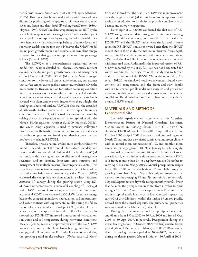
During the experiments, cumulative precipitation was 41 and 61 mm from 1 Oct. 2005 to 30 Apr. 2006 and from 1 Oct. 2006 to 30 Apr. 2007, respectively. Precipitation during the initial freezing (about 1 October–30 November) and the frozen period (about 1 December–10 March) of 2005–2006 was more than that during the same period of 2006–2007, but was less during the thawing period (about 11 March– 30 April) of 2005–

1550 Soil Science Society of America Journal

2006 than that of 2006–2007 (Fig. 1). The frozen period lasted more than 3 mo and had minimum air temperatures of –33.4°C for 2005–2006 and –28.4°C for 2006–2007 (Fig. 1).

Experimental Treatments and ManagementThe experimental design included two plots receiving no

irrigation before winter (CK) and two plots receiving irrigation

before winter in later October to bring the soil water storage in the 0- to 60-cm profile to field capacity (WI). All four plots were arranged in a randomized design with two replications, namely CK01, CK02, WI01, and WI02, and planted in Siberian wildrye (Elymus sibiricus L.), a perennial forage crop with high drought and cold tolerance widely planted in this region (Dong et al., 2007; Chen and He, 2004).

Table 1. Calibrated soil hydraulic properties for both RZ-SHAW and SHAW models using data from 2005–2006.

DepthBulk

densityl for

RZWQM†b for

SHAW†Bubbling pressure†

Saturated hydro-

conductivity

Field capacity† (1/3Bar)

Wilting point† (15Bar)

Saturated water

content

Particle size distribution Organic

matterpH

Electrical conductivity

Sand Silt Clay

cm kg m–3 m cm h–1 –––––– m3 m–3 –––––– –––– % –––– g kg–1 mS cm–1

0–15 1400 0.215 4.65 –0.43 1.83 0.303 0.134 0.472 70 17 13 28.94 8.20 0.15

15–30 1490 0.179 5.60 –0.40 2.10 0.300 0.152 0.438 72 16 12 25.07 8.32 0.15

30–45 1630 0.149 6.71 –0.32 2.25 0.271 0.154 0.385 76 13 11 16.89 8.42 0.1545–65 1590 0.144 6.54 –0.20 2.21 0.266 0.154 0.400 79 10 11 6.67 8.48 0.14† l is pore size distribution index in the modified Brooks–Corey model (BC model), b is pore size distribution index in the modified Campbell

model (C model), and Bubbling pressure units are centimeters in the BC model and meters in the C model. The parameters l, b, bubbling pressure, field capacity, and wilting point were calibrated based on the measured values during the simulation.

Fig. 1. Air temperature and precipitation during (a) 2005–2006 and (b) 2006–2007.


Seedbeds were conventionally tilled. Siberian wildrye was sown using a drill with a row spacing of 33 cm on 15 June 2005 at a seeding rate of 25 kg ha–1and a seeding depth of 3 to 5 cm. The plot size was 8 m wide by 20 m long, and there was a 1.5-m wide buffer zone between plots to minimize interference between treatments. Water was applied by a removable sprinkler system mounted on a rubber pipe. Two sprinklers were located on both sides of the irrigated plots. This system was designed to ensure uniform water coverage and distribution. The irrigation amount was calculated based on the irrigated area and water volume from a water meter. The equivalent depth of water applied was 26 mm (WI01) and 31 mm (WI02) on 18 Oct. 2005, and 57 mm (WI01) and 49 mm (WI02) on 19 Oct. 2006, respectively. Chemical fertilizers (75 kg ha–1 N and 20 kg ha–1

P) were incorporated in the top 10-cm soil layer before seeding in 2005 and again applied on the soil surface in May of both years.

MeasurementsDry mass and thickness of surface residue layer along

with fraction of surface residue cover were measured in late September after harvest. The aboveground residue was collected in an area of 3 × 3 m for dry mass measurement. The residue samples were oven-dried at 75°C for 72 h (Ercoli et al., 1999). Total soil volumetric water content in the 0- to 15-, 15- to 30-, 30- to 45- and 45- to 60-cm soil depths were measured by sampling soil with a soil auger (20 mm inner diameter) every 2 mo during winter. Liquid water contents were measured in situ by time domain reflectometry (TDR) using TDR100 (Campbell Scientific, Logan, UT) with

Fig. 2. Relationship between measured and simulated (a and b) soil total water content and (c and d) total water storage for non-irrigation (CK) and winter irrigation (WI) treatments using RZ-SHAW and SHAW combing two plots of each treatment and two winters.


CS605 probes with three rods horizontally installed at soil depths of 7.5, 22.5, 37.5, 52.5, and 62.5 cm. Soil temperatures were measured in situ with thermocouples (AV-10T, Avalon Scientific, Jersey City, NJ) horizontally installed at the same soil depths as the CS605 probes. Liquid water content equaled total water content in unfrozen soil. Liquid water contents and soil temperatures were measured at 0900 h every 3 to 5 d. The freeze and thaw depths in the 0- to 150-cm profile were monitored by frost-tubes every 3 d. Air temperature, wind speed, relative humidity, precipitation, and sunshine hours were measured hourly at the nearest meteorological station (Guyuan Station, elevation of 1412 m) located 20 km from the experimental site, since no weather data were recorded during winter on the experiment site. Incoming shortwave

radiation was calculated with the Angstrom formula, which relates solar radiation to extraterrestrial radiation and relative sunshine duration, in FAO 56 (Allen et al., 1998). Precipitation was measured at the experimental site during the growing season. Camargo and Hubbard (1999) reported that for a separation distance of 50 km between two weather stations in the United States high plains, there were lesser standard errors for the solar radiation (0.8–2.0 MJ m–2) and potential ET (0.3–0.8 mm) from October to March than during the other months, and that the standard errors of maximum and minimum air temperature were from 1.0 to 2.0°C. Differences in precipitation and air temperature between the Guyuan Station and the experimental site may partially be responsible for the simulation errors in this study.

Fig. 3. Comparison of measured and simulated total water content for (a) non-irrigation and (b) winter irrigation treatments using RZ-SHAW and SHAW during 2006–2007 period.


Development of the RZ-SHAW ModelThe RZ-SHAW uses routines from the SHAW model to

simulate the energy balance in the canopy, residue, snowpack, and soil layers; soil water freezing and thawing or ice content; and soil temperature, while keeping its own soil water movement routines using the Green–Ampt equation for infiltration and the Richards equation for soil liquid water redistribution (Ahuja et al., 2000). The SHAW routines are called only during the redistribution phase of water movement. In RZ-SHAW model, the evaporative flux from solving the Richards equation in RZWQM routines is exported to the SHAW routines for latent heat and soil temperature calculations. Since plant transpiration is calculated as part of the canopy energy balance in SHAW, RZWQM routines import the simulated transpiration from SHAW routines at each time step to make sure that the simulated ET in RZWQM routines agree with the latent heat from SHAW routine (Ma et al., 2012a). At each time step of solving the Richards equation, RZWQM routines provide the SHAW routines with evaporation flux, liquid soil water content, and plant information (leaf area index, plant height, and rooting depth). In return, the SHAW routines provide RZWQM routines with soil temperature, updated liquid water content after freeze-and-thaw adjustment, and

transpiration flux to be used at the next time step, along with all components of energy balance (latent heat, sensible heat, ground heat flux, and total net radiation).

Since the SHAW model and the RZ-SHAW model simulate rainfall infiltration using the Green–Ampt equation and water redistribution by solving the Richards equation, the difference between RZ-SHAW and SHAW is minimal in water movement. In RZ-SHAW, the actual evaporation flux is determined by the ability of soil surface water flux (by solving the Richards equation) to meet a potential evaporation estimated by the Shuttleworth–Wallace equation (Ahuja et al., 2000), whereas the SHAW evaporation is calculated by vapor pressure differences between soil and air. Another difference between RZ-SHAW and SHAW is in the freezing-and-thawing process. Although RZ-SHAW model uses the same routine as in SHAW, we have to limit the minimum water potential for soil freeze to the same minimum potential (i.e., –35,000 cm) for solving the Richards equation in the RZWQM routines. The SHAW uses the actual vapor pressure as the boundary condition in solving the Richards equation without the need to specify a minimum soil water potential. The third difference between RZ-SHAW and SHAW is that the energy balance and the soil freeze-and-thaw subroutines are called only during the redistribution phase

Table 2. Model performance for simulated total water content and soil water storage during the two winters (October–April).

Year DepthCK01 plot CK02 plot WI01 plot WI02 plot

RMSD† ME RMSD ME RMSD ME RMSD ME

cmRZ-SHAW

2005–2006 7.5 0.017 –0.50 0.014 0.06 0.030 0.34 0.031 0.32

22.5 0.043 –8.36 0.025 –8.70 0.030 –1.02 0.055 –2.02

37.5 0.030 –9.51 0.036 –13.12 0.045 –4.91 0.058 –2.0852.5 0.012 –2.00 0.021 –0.10 0.049 –12.77 0.035 0.22

Mean 0.026 –5.09 0.024 –5.47 0.038 –4.59 0.045 –0.89SWS‡ 0–60 5.4 –2.60 11.1 –2.38 9.1 0.45 19.1 –0.70

2006–2007 7.5 0.019 0.65 0.020 0.52 0.032 0.64 0.031 0.46

22.5 0.015 –3.16 0.023 –18.73 0.030 0.77 0.042 0.26

37.5 0.025 –65.94 0.014 –3.43 0.040 0.46 0.026 0.5452.5 0.016 –9.30 0.018 –6.26 0.051 –3.97 0.033 0.09

Mean 0.019 –19.44 0.019 –6.97 0.038 –0.52 0.033 0.34SWS 0–60 8.6 –2.14 8.2 –2.88 9.0 0.89 10.7 0.73

SHAW

2005–2006 7.5 0.016 –0.44 0.036 –5.57 0.020 0.70 0.050 –0.80

22.5 0.042 –7.56 0.024 –7.65 0.015 0.52 0.050 –1.48

37.5 0.033 –11.31 0.032 –10.40 0.034 –2.39 0.061 –2.3252.5 0.024 –10.94 0.019 0.09 0.071 –27.50 0.029 0.45

Mean 0.029 –7.56 0.028 –5.88 0.035 –7.17 0.047 –1.04SWS 0–60 6.3 –3.84 8.9 –1.16 5.3 0.81 15.6 –0.14

2006–2007 7.5 0.020 0.61 0.025 0.26 0.037 0.54 0.080 –2.57

22.5 0.016 –3.44 0.024 –21.16 0.021 0.89 0.032 0.56

37.5 0.023 –53.23 0.014 –3.31 0.035 0.59 0.025 0.5752.5 0.018 –11.69 0.020 –7.83 0.063 –6.49 0.039 –0.28

Mean 0.019 –16.94 0.020 –8.01 0.039 –1.12 0.044 –0.43SWS 0–60 8.5 –2.03 9.3 –4.01 9.6 0.88 18.5 0.18† RMSD, root mean square difference, mm for SWS and m3 m–3 for soil water content; ME, model efficiency.‡ SWS, soil water storage.


of water movement in the RZ-SHAW model, which was shown to not be a problem in several previous tests of RZ-SHAW (Yu et al., 2007; Ma et al., 2012a).

Models SimulationsRZ-SHAW and SHAW simulations were performed for

two winters from 1 Oct. 2005 to 28 Apr. 2006 and from 6 Oct. 2006 to 25 Apr. 2007 using hourly meteorological data. Soil water retention parameters were calculated based on measured soil temperature and liquid water content in the two WI plots from October 2005 to April 2006 using the approach outlined by Flerchinger et al. (2006), and validated with the data set from October 2006 to April 2007. The soil water retention curve is described by Brooks–Corey equation (Eq.[1]) in RZ-SHAW models and by Campbell equation (Eq.[2]) in SHAW.

(θ – θr)/( θs – θr ) = (h/hb)–λ [1]

ψ = ψe(θ/ θs)–b [2]

Here, θ, θr, and θs are volumetric soil water content (m3 m–3), residual water content (m3 m–3, assumed to be 0), and satu-rated soil water content (m3 m–3), respectively. Ψ and ψe are matric potential (m) and air-entry potential (m), respectively. h and hb are pressure head (m) and air-entry pressure head (m), λ is the pore size distribution index in the Brooks–Corey equation and b is the pore size distribution index in modified Campbell equation (λ = 1/b). The two equations are equiva-lent when the residual water content is assumed to be zero in the Campbell equation. Parameters were calibrated based on

Fig. 4. Comparison of measured and simulated soil total water storage for (a) non-irrigation and (b) winter irrigation treatments using RZ-SHAW and SHAW for the 2005–2006 and 2006–2007 winter periods.


total water content and liquid water content for the simulated period in the 2005–2006 (Table 1).

The models were initialized with measured soil water content and soil temperature. Initial residue was 0.9 t ha–1 with 5 cm height and 50 d age for the period of 2005–2006, and 1.8 t ha–1 with 10 cm height and 50 d age for the 2006–2007 simulation period. Fraction of surface residue coverage was 0.5 m2 m–2 in the SHAW model and was calculated in the RZ-SHAW based on residue weight. Albedo value of residue was set at 0.25 m2 m–2 for all models runs.

Model efficiency (ME) and root mean squared deviation (RMSD) were used to evaluate model performance. The ME is analogous to the coefficient of determination (r2), with the

exception that ME ranges from negative infinity to 1.0; negative ME values indicate that the mean observation is a better predictor than simulated values (Eq. [3]). RMSD is a measure of the absolute difference between simulated and measured values (Eq. [4]).

2

1

2

1

( )ME 1

( )

ˆN

i iiN

ii

Y YY Y

[3]

1/22

1

1RMSD ( )ˆN

i iiN Y Y

[4]

Fig. 5. Relationship between measured and simulated (a and b) soil liquid water content and (c and d) liquid water storage for non-irrigation (CK) and winter irrigation (WI) treatments using RZ-SHAW and SHAW combing two plots of each treatment and two winters.


Here, Y i is the simulated value, Yi is the observed value, Y is the mean of observed values, and N is the number of observation.

RESULTS AND DISCUSSIONSimulation of Total Water Content

For the non-irrigation treatment, total soil water content in each soil layer was better simulated than under irrigation treatment for both models possibly due to smaller variations in soil water content under non-irrigation treatment (Fig. 2a, 2b, and 3). For the RZ-SHAW model, the average RMSD was 0.025 m3 m–3 in 2005–2006, and 0.019 m3 m–3 in 2006–2007 for the non-irrigation treatment, and 0.039 m3 m–3 for both years for the irrigation treatment (Table 2). For the SHAW model, average RMSD was 0.029 m3 m–3 in 2005–2006, and 0.020 m3 m–3 in 2006–2007 under non-irrigation condition, respectively. It was 0.041 m3 m–3 and 0.042 m3 m–3 for the two winter periods under irrigation condition (Table 2). As

shown in Fig. 3, RZ-SHAW under predicted total soil water content at the soil surface, which may be partially due to overprediction of soil evaporation by RZ-SHAW to meet the potential evaporation estimated by the Shuttleworth–Wallace equation. Overprediction of soil evaporation by RZWQM was also reported by Fang et al. (2010). In contrast, the SHAW underpredicted soil evaporation, which could have resulted in overprediction of surface soil water content (Fig. 3). Nonetheless, simulated total water content with the RMSD from 0.012 to 0.058 m3 m–3 by RZ-SHAW was comparable to the RMSD range from 0.020 to 0.070 m3 m–3 in Flerchinger et al. (2000). The simulated RMSD range from 0.014 to 0.080 m3 m–3 by SHAW was similar to the RMSD of 0.018 to 0.050 m3 m–3 in Kozak et al. (2007).

Simulated total soil water storage in the top 60-cm soil profile for the non-irrigation treatment between the two models were very close to the experimental measurements (Fig. 2c).

Fig. 6. Comparison of measured and simulated liquid water content for (a) non-irrigation and (b) winter irrigation treatments using RZ-SHAW and SHAW during the 2006–2007 winter period.


However, there was considerable difference between the two models in simulating soil water storage for the pre-winter irrigation treatment (Fig. 4), notably after the freezing period under irrigation treatment. The RMSD of total soil water storage simulated by RZ-SHAW ranged from 5.4 to 11.1 mm in 2005–2006 and from 8.2 to 8.6 mm in 2006–2007 for the non-irrigation treatment, and from 9.1 to 19.1 mm in 2005–2006 and from 9.0 to 10.7 mm to 2006–2007 for the irrigation treatment. Correspondingly, RMSD from SHAW model ranged from 6.3 to 8.9 mm in 2005–2006 and from 8.5 to 9.3 mm in 2006–2007 for the non-irrigation treatment, and from 5.3 to 15.6 mm in 2005–2006 and from 9.6 to 18.5 mm in 2006–2007 for the irrigation treatment (Table 2). Both models better simulated soil water storage under the non-irrigation treatment than under the irrigation treatment (Fig. 2c, 2d, and 4). The RZ-SHAW model under predicted soil water storage for the irrigation treatments in 2005–2006 season, whereas the SHAW model overpredicted total water storage in the 2006–2007 season. Both models underestimated total soil water storage in early spring of 2006 during the thawing stage for the CK02 and WI02 treatments (Fig. 4). One possible reason may be that the high initial soil water before the winter in 2005–2006 resulted in overestimation of ET by RZ-SHAW model during the freezing

period, which resulted in underestimation of soil water storage in the 2005–2006 season. Nonetheless, overall performance of the two models was very similar as reported by Flerchinger et al. (2000), Kozak et al. (2007), and Ma et al. (2012a).

Model efficiency of simulated total water content for most soil layers were either negative or <0.5 (Table 2) which resulted from relatively small variations of total water content from 0.10 to 0.35 m3 m–3 (Fig. 4) and relatively large simulation errors with RMSD from 0.012 to 0.080 m3 m–3 (Table 2). It is interesting to note that ME for the irrigation treatment were better than those for the non-irrigation treatment in spite of larger RMSD for the irrigation treatment. Therefore, the results of ME in simulation of total water content are not good because only two data points were measured during the frozen period and may not reflect the variations of total water content. Low ME for simulation of soil water content was also found in Ma et al. (2012b).

Simulation of Liquid Water ContentBoth models provided acceptable simulations of liquid

water content for all soil layers except for the two bottom soil layers (Fig. 5a, 5b, and 6) while generally performing better for the non-irrigation treatment than for the irrigation treatment (Fig. 5a). Both models underestimated liquid soil water after

Table 3. Model performance for simulated liquid water content and soil liquid water storage during the two winters (October–April).



cmRZ-SHAW

2005–2006 7.5 0.017 0.72 0.021 0.72 0.034 0.57 0.030 0.6222.5 0.035 0.52 0.024 0.80 0.025 0.79 0.041 0.59

37.5 0.033 –1.76 0.030 0.70 0.037 0.59 0.040 0.5552.5 0.023 0.02 0.020 0.80 0.055 –8.11 0.030 0.69

Mean 0.027 –0.13 0.024 0.75 0.038 –1.54 0.035 0.61SWS‡ 0–60 7.2 0.83 11.4 0.82 12.1 0.78 16.2 0.71

2006–2007 7.5 0.018 0.60 0.014 0.71 0.029 0.63 0.022 0.70

22.5 0.009 0.51 0.018 0.01 0.025 0.80 0.026 0.75

37.5 0.029 –42.28 0.014 0.32 0.036 0.60 0.028 0.6752.5 0.020 –25.91 0.019 –1.03 0.059 –6.64 0.028 0.68

Mean 0.019 –16.77 0.016 0.00 0.037 –1.15 0.026 0.70SWS 0–60 8.9 –1.00 8.2 0.31 10.8 0.82 11.9 0.78

SHAW

2005–2006 7.5 0.014 0.81 0.020 0.76 0.014 0.92 0.029 0.64

22.5 0.033 0.56 0.020 0.86 0.022 0.84 0.036 0.69

37.5 0.037 –2.31 0.026 0.77 0.031 0.71 0.037 0.6152.5 0.030 –0.68 0.019 0.81 0.070 –13.66 0.025 0.78

Mean 0.028 –0.41 0.021 0.80 0.034 –2.80 0.032 0.68SWS 0–60 9.3 0.72 9.3 0.88 13.5 0.72 12.5 0.83

2006–2007 7.5 0.017 0.58 0.017 0.56 0.024 0.75 0.051 –0.68

22.5 0.010 0.33 0.021 –0.32 0.031 0.68 0.039 0.43

37.5 0.028 –37.94 0.015 0.27 0.032 0.69 0.032 0.5652.5 0.022 –32.74 0.020 –1.10 0.072 –10.12 0.033 0.55

Mean 0.019 –17.44 0.018 –0.15 0.040 –2.00 0.039 0.21SWS 0–60 9.9 –1.56 10.1 –0.03 16.6 0.56 20.4 0.34† RMSD, root mean square difference, mm for SWS and m3 m–3 for soil water content; ME, model efficiency.‡ SWS, soil liquid water storage.


irrigation and during thawing for the 30- to 45-cm soil layer, but overestimated liquid soil water for the 45- to 60-cm soil layer during the same periods, which suggested that the models simulated too much water draining from the 30- to 45-cm soil layer to the 45- to 60-cm soil layer (Fig. 6). Such an over charge of liquid soil water between soil layers may be corrected by reducing the soil hydraulic conductivity or increasing the field capacity for the 30- to 45-cm soil layer. The increase in liquid water in the subsurface soil layers in early spring showed that both models predicted a rapid thawing process, which corresponded to the quick disappearance of frozen depth as discussed later. In terms of RMSD, simulated liquid water content by both models was comparable (Table 3). Model efficiency of liquid water content simulation for most soil layers were above 0.5 (Table 3), which also suggested that the model performance was acceptable.

For the non-irrigation treatment, both models yielded good simulations of liquid water storage (Fig. 5c and 7) with mean RMSD values for CK01 and CK02 plots ranging from 8.6 to 9.3 mm for RZ-SHAW and from 9.3 to 10.0 mm for SHAW (Table 3). For the non-irrigation treatment, the RMSD of simulated liquid water storage ranged from 7.2 to 11.4 mm for 2005–2006 and from 8.2 to 8.9 mm for 2006–2007 by RZ-SHAW, and 9.3 mm for 2005–2006 and from 9.9 to 10.1 mm for 2006–2007 by SHAW (Table 3). Simulated RMSD of liquid water storage were larger for the irrigation treatment for both models (Table 3, Fig. 5d and 7). Again, the discrepancy between simulated and measured total liquid water content was due to rapid thawing of ice in the lower soil layers simulated by both models. Since goodness of simulation of liquid water content varied from plot to plot and from year to year, there was no agreement on which model was better than the other (Table 3).

Fig. 7. Comparison of measured and simulated liquid water storage for (a) non-irrigation and (b) winter irrigation treatments using RZ-SHAW and SHAW for the 2005–2006 and 2006–2007 periods.


Simulation of Soil TemperatureRZ-SHAW simulated soil temperature slightly better than

SHAW (Fig. 8 and 9). The accuracy of soil temperature prediction increased with soil depth for both models, probably because the measured soil temperature at 62.5 cm was used as the lower boundary condition in both models (Table 4, Fig. 8 and 9). Both

models simulated more temperature fluctuation at the soil surface than measured values, which could be due to less frequent sampling (Fig. 9). For two soil layers beneath the soil surface, both models simulated higher temperature than experimentally measured, which may be the cause for the simulated early and rapid thawing. On average, RZ-SHAW simulated better soil

Fig. 8. Relationship of measured and simulated soil temperature for winter irrigation (WI) treatment using RZ-SHAW and SHAW.


temperature than the SHAW model for all the four plots in both years (Table 4). The slightly worse prediction by the SHAW model was attributed to an overestimation of soil temperature during the freezing and part of the frozen period, and underestimation of soil temperature during part of the frozen and thawing period (Fig. 9). Such discrepancy in soil temperature simulation by SHAW could be partially due to a fixed percentage residue cover used in the SHAW, whereas the RZ-SHAW model calculates residue coverage based on surface residue mass that varies from time to time during our experimental period (Farahani and DeCoursey, 2000). In addition, RZ-SHAW provided more consistent prediction between the two winter periods than the SHAW model (Table 4). Simulated soil temperature with RMSD from 0.5 to 2.9°C by RZ-SHAW was comparable to the results of the RMSD of 2.18 and 2.23°C at both 1.5- and 4.5-cm depths from Ma et al. (2012a) and the RMSD from 1.43 to 2.49°C in Kozak et al. (2007). The RMSD of soil temperature

from 0.5 to 4.2°C by SHAW was also comparable to the results of the RMSE from 0.4 to 4.4°C in Flerchinger et al. (2000). The ME was much better than total soil water and liquid water simulations (ME = 0.74–0.99) (Table 4), which was mainly due to a large variation in soil temperature measurements during the simulation periods (Fig. 9).

Simulation of Freeze and Thaw DepthsRZ-SHAW and SHAW models provided good simulations

for soil freeze depth on all plots except for the CK01 plot during 2006–2007, but poor simulations for the thaw depth (Fig. 10). It seems that the entire frozen soil disappeared suddenly at the beginning of spring, which could be due to lower ice content simulated in the soil profile. Another possible reason was the higher temperature simulated in early spring (Fig. 9). The reason that a thaw depth of 3 to 10 cm was simulated by SHAW during the frozen period (e.g., non-irrigation treatment) was due to the

Fig. 9. Comparison of measured and simulated soil temperature for (a) non-irrigation and (b) winter irrigation treatments using RZ-SHAW and SHAW during the 2006–2007 period.


low soil water content of <0.10 m3 m–3 in winter. Ice formation in such a dry soil requires soil temperature well below 0°C (Flerchinger and Saxton, 1989b). Otherwise, no ice was formed because soil water was hygroscopic water with a much lower freezing point.

The measured temperature differences between irrigation and non-irrigation treatments were statistically significant during the simulated period (mean p = 0.523), specially for surface soil. Soil temperature increase due to irrigation in the winter was better simulated by the SHAW model than by the RZ-SHAW model, which could be attributed to lower simulated soil water content in the RZ-SHAW model (Fig. 4). The difference between treatments was only 1 to 2°C during the frozen and thawing periods, which was within the simulation error of 1 to 4°C. Therefore, it was difficult to simulate soil temperature difference resulting from irrigation practice.

CONCLUSIONSAs expected, RZ-SHAW model showed similar performance

compared to the original SHAW model in simulating total water content, liquid water content, and soil temperature. The average RMSD for RZ-SHAW model was 0.030 m3 m–3 for total water content, 0.028 m3 m–3 for liquid water content, and 1.4°C for soil temperature. Both models provided better simulations of total soil water and liquid soil water under non-irrigation than under irrigation treatment, but the simulations of soil temperature were similar for all plots. The mean RMSD for total water content was 0.022 m3 m–3 under non-irrigation and 0.039 m3 m–3

under irrigation treatment, 0.022 and 0.034 m3 m–3 for liquid water content, and 1.5 and 1.4°C for soil temperature. Both RZ-SHAW and SHAW simulated the soil freezing process well, but the simulation of soil thawing process was poor. The results demonstrated that the SHAW routines were incorporated into RZWQM correctly, which makes the hybrid model, RZ-SHAW, a better tool for simulating winter conditions (soil water and soil temperature) and their effects on plant growth in future studies. However, we do not expect RZ-SHAW to improve the simulation of soil water and temperature in the winter over that of SHAW because of the similarity between the two models in soil water movement. Future work should evaluate RZ-SHAW for simulating the growth of winter crops (e.g., winter wheat).

ACKNOWLEDGMENTSThis work was supported by the National Natural Science Foundation of China (no. 30471228, no. 41128001 and no. 41071153) and the National Key Technology Research and Development Program (no. 2006BAD16B01). We also appreciate researchers at the National Grassland Ecosystem Station located in Bashang Plateau, Hebei Province, for their help with the field experiments.

REFERENCESAhuja, L.R., K.W. Rojas, J.D. Hanson, M.J. Shaffer, and L. Ma. 2000. Root Zone

Water Quality Model: Modeling management effects on water quality and crop productivity. Water Resour. Publ., Highlands Ranch, CO.

Allen, R.G., L.S. Pereira, D. Raes, and M. Smith. 1998. Crop evapotranspiration: Guidelines for computing crop water requirements. Irrigation and Drainage Paper 56. FAO, Rome.

Camargo, M.B.P., and K.G. Hubbard. 1999. Spatial and temporal variability of daily weather variables in sub-humid and semi-arid areas of the united

Table 4. Model performance for simulated soil temperature during the two winters (October–April).



cmRZ-SHAW

2005–2006 7.5 2.9 0.80 2.5 0.83 2.3 0.85 2.5 0.82

22.5 1.3 0.95 1.4 0.94 1.4 0.94 1.3 0.95

37.5 1.2 0.95 1.0 0.96 1.4 0.92 1.1 0.9652.5 0.5 0.99 0.8 0.98 0.5 0.99 0.5 0.99

Mean 1.5 0.92 1.4 0.93 1.4 0.93 1.3 0.93

2006–2007 7.5 2.8 0.88 2.6 0.90 2.4 0.90 2.3 0.91

22.5 1.5 0.95 1.5 0.95 1.6 0.95 1.2 0.97

37.5 1.3 0.96 1.0 0.98 1.2 0.97 1.0 0.9852.5 0.9 0.98 0.5 0.99 0.6 0.99 0.7 0.99

Mean 1.6 0.94 1.4 0.95 1.4 0.95 1.3 0.96

SHAW

2005–2006 7.5 2.4 0.86 2.3 0.86 2.1 0.88 1.9 0.89

22.5 2.1 0.87 2.0 0.87 1.8 0.90 1.5 0.93

37.5 1.3 0.94 1.0 0.96 1.3 0.94 1.0 0.9652.5 0.6 0.98 0.7 0.98 0.5 0.99 0.6 0.99

Mean 1.6 0.92 1.5 0.92 1.4 0.92 1.3 0.94

2006–2007 7.5 4.2 0.74 4.1 0.74 3.3 0.81 3.3 0.81

22.5 2.9 0.82 2.4 0.87 2.6 0.86 2.4 0.87

37.5 1.5 0.95 1.6 0.93 1.2 0.96 1.6 0.9452.5 0.7 0.99 0.8 0.98 0.7 0.99 1.0 0.97

Mean 2.3 0.87 2.2 0.88 2.0 0.91 2.1 0.90† RMSD, root mean square difference, °C; ME, model efficiency.


states high plains. Agric. For. Meteorol. 93:141–148. doi:10.1016/S0168-1923(98)00122-1

Chen, G., and L.F. He. 2004. Evaluation of ecological adaptability and productivity of two species of Elymus in alpine region. (In Chinese with English abstract.) Pratacultural Sci. 21:39–42.

Dong, S.K., M.Y. Kang, X.J. Yun, R.J. Long, and Z.Z. Hu. 2007. Economic comparison of forage production form annual crops, perennial pasture and native grassland in the alpine region of the Qinghai-Tibetan Plateau, China. Grass Forage Sci. 62:405–415. doi:10.1111/j.1365-2494.2007.00594.x

Ercoli, L., M. Mariotti, A. Masoni, and E. Bonari. 1999. Effect of irrigation and nitrogen fertilization on biomass yield and efficiency of energy use in crop

production of Miscantbus. Field Crops Res. 63:3–11.Fang, Q.X., T.R. Green, L. Ma, R.W. Malone, R.H. Erskine, and L.R. Ahuja.

2010. Optimizing soil hydraulic parameters in RZWQM2 using automated calibration methods. Soil Sci. Soc. Am. J. 74:1897–1913. doi:10.2136/sssaj2009.0380

Farahani, H.J., and D.G. DeCoursey. 2000. Evaporation and transpiration processes in the soil-residue-canopy system. In: L.R. Ahuja, K.W. Rojas, J.D. Hanson, M.J. Shaffer, and L. Ma, editors, The Root Zone Water Quality Model. Water Resources Publ., Highlands Ranch, CO. p. 51–80.

Flerchinger, G.N., R.M. Aiken, K.W. Rojas, and L.R. Ahuja. 2000. Development

Fig. 10. Comparison of measured and simulated freeze and thaw depths using (a) RZ-SHAW and (b) SHAW for the 2005–2006 and 2006–2007 periods.


of the root zone water quality model (RZWQM) for over-winter conditions. Trans. ASAE 43(1):59–68.

Flerchinger, G.N., and K.E. Saxton. 1989a. Simultaneous heat and water model of a freezing snow-residue-soil system I. Theory and development. Trans. ASAE 32(2):565–571.

Flerchinger, G.N., and K.E. Saxton. 1989b. Simultaneous heat and water model of a freezing snow-residue-soil system II. Field verification. Trans. ASAE 32(2):573–578.

Flerchinger, G.N., M.S. Seyfried, and S.P. Hardegree. 2006. Using soil freezing characteristic to model multi-season soil water dynamics. Vadose Zone J. 5:1143–1153. doi:10.2136/vzj2006.0025

Hayhoe, H.N. 1994. Field testing of simulated soil freezing and thawing by the SHAW model. Can. Agric. Eng. 36(4):279–285.

Jame, Y., and D.I. Norum. 1980. Heat and mass transfer in a freezing unsaturated porous medium. Water Resour. Res. 16(4):811–819. doi:10.1029/WR016i004p00811

Kozak, J.A.R.M., G.N. Flerchinger, D.C. Nielsen, L. Ma, and L.R. Ahuja. 2007. Comparison of modeling approaches to quantify residue architecture effects on soil temperature and water. Soil Tillage Res. 95:84–96. doi:10.1016/j.still.2006.11.006

Lauriault, L.M., R.E. Kirksey, and G.B. Donart. 2002. Irrigated and nitrogen effects on tall wheatgrass yield in the Southern High Plains. Agron. J. 94:792–797. doi:10.2134/agronj2002.0792

Lauriault, L.M., R.E. Kirksey, and D.M. van Leeuwen. 2005. Performance of perennial cool- season forage grasses in diverse soil moisture environments, southern high plains, USA. Crop Sci. 45:909–915. doi:10.2135/cropsci2004.0280

Li, Z., and H. Wang. 2010. Effects of winter irrigation on soil moisture and thermal condition of artificial grassland during the winter in agro-pastoral ecotone of China. (In Chinese with English abstract.) Agric. Res. in the Arid Areas 28(4):7–13.

Ma, L., L.R. Ahuja, B.T. Nolan, R.W. Malone, T.J. Trout, and Z. Qi. 2012b. Root Zone Water Quality Model (RZWQM2): Model use, calibration and validation. Trans. ASABE (In press.)

Ma, L., G.N. Flerchinger, L.R. Ahuja, T.J. Saucer, J.H. Prueger, R.W. Malone, and J.L. Hatfield. 2012a. Simulating the surface energy balance in a soybean canopy with SHAW and RZ-SHAW models. Trans. ASABE 55:175–179.

Yu, Q., G.N. Flerchinger, S. Xu, J. Kozak, L. Ma, and L. Ahuja. 2007. Energy balance simulation of a wheat canopy using the RZ-SHAW (RZWQM-SHAW) model. Trans. ASABE 50(5):1507–1516.

Documents

Soil Physics Simulation of Overwinter Soil Water and Soil …. zizhon… · · 2017-08-02viving through the cold winter (Lauriault et al., 2002; Lauriault et al., 2005). ... and