Contents lists available at ScienceDirect

Soil Dynamics and Earthquake Engineering

journal homepage: www.elsevier.com/locate/soildyn

Empirical correlations between the effective number of cycles and otherintensity measures of ground motions

Wenqi Dua,⁎, Gang Wangb

a Institute of Catastrophe Risk Management, Nanyang Technological University, 50 Nanyang Avenue Singaporeb Dept. of Civil and Environmental Engineering, The Hong Kong University of Science and Technology, Clear Water Bay, Kowloon Hong Kong

A R T I C L E I N F O

Keywords:Effective number of cyclesCorrelation coefficientNGA databaseGround motion selectionLiquefaction potential

A B S T R A C T

The effective number of cycles is an important ground motion parameter for the assessment of liquefactionpotential. In this paper, empirical correlations for two measures of the effective number of cycles with sevenamplitude-, cumulative-, and duration-based intensity measures (IMs) are studied and compared, based on theNGA strong motion database and several ground motion prediction equations. The adopted definitions of theeffective number of cycles include an absolute measure (NA) and a relative measure (NR). It is shown that NA ishighly correlated with high-frequency IMs, such as spectral acceleration (SA) at short periods, Arias intensity,and negatively correlated with signification durations (Ds). On the other hand, NR shows generally negativecorrelations with both amplitude- and cumulative-based IMs. NR also exhibits small-to-moderate positive cor-relations with Ds, which are commonly regarded as similar parameters to the effect number of cycles. Simpleparametric functions are provided to describe the NA-SA and NR-SA correlations for various cases. The im-portance of considering multiple IMs rather than SA only in ground-motion selection is also briefly demon-strated.

1. Introduction

The number of cycles of ground motions has been widely recognizedas one of the critical parameters in geotechnical earthquake en-gineering. Many studies (e.g., [1,2]) have concluded that the number ofcycles of shakings is strongly correlated with the buildup of pore waterpressure in liquefiable soils. As summarized by Hancock and Bommer[3], there are dozens of definitions to count the effective number ofcycles, by converting all irregular amplitude cycles to an equivalentnumber of uniform cycles. The concept of equivalent number of cyclesis commonly used for evaluating liquefaction potential [4–6].

Due to the complex features of ground motion time histories, singleground motion intensity measure (IM) cannot adequately characterizeearthquake loadings. Therefore, a set of IMs (vector-IMs) is often re-quired in some practical applications, such as the estimation of earth-quake-induced slope displacement [7,8]. Since current ground motionprediction equations (GMPEs) only provide the means and standarddeviations for specific IMs, empirical correlations among the residualsof these IMs are then the key requirement to contrast the joint dis-tribution of vector-IMs. These empirical correlations are indispensablein vector-based probabilistic seismic hazard analysis [9] and scenario-based ground motion selection approaches, e.g., [10–12].

Recently a number of researchers have studied empirical correla-tions between the residuals of multiple IMs, such as spectral accelera-tions (SA) at multiple periods, Arias intensity (Ia), cumulative absolutevelocity (CAV), and significant durations (Ds), e.g., [13–18]. However,to the knowledge of the authors, there are no existing correlationmodels involving the number of effective cycles. Bommer et al. [19] hasstudied the correlations between several duration parameters and ef-fective numbers of ground motion cycles. Yet, they did not aim atevaluating the correlations between the residuals of these IMs, makingit difficult to be used in some applications such as ground motion se-lection.

The objective of this paper is to examine the empirical correlationsbetween the effective number of cycles and other commonly used IMs.The definitions of these employed IMs are firstly discussed, associatedwith the utilized GMPEs and ground motion database. Secondly, theestimated correlation coefficients between the residuals of these IMs arepresented; simple parametric models are also proposed to readily pre-dict the empirical correlations. The influence of rupture distance (Rrup)on the resulting correlation coefficients is then examined. Finally, basedon the correlation results, some recommendations are provided re-garding the use of different definitions of the effective number of cyclesfor practical applications.

http://dx.doi.org/10.1016/j.soildyn.2017.08.014Received 17 November 2015; Received in revised form 9 July 2017; Accepted 25 August 2017

⁎ Corresponding author.E-mail address: wqdu@ntu.edu.sg (W. Du).

Soil Dynamics and Earthquake Engineering 102 (2017) 65–74

0267-7261/ © 2017 Elsevier Ltd. All rights reserved.

MARK

2. Selected IMs and ground motion database

2.1. Effective number of cycles

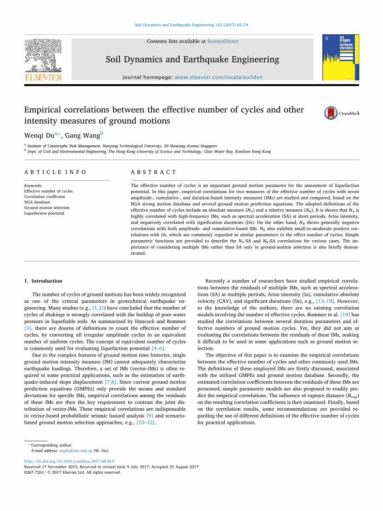
As summarized in Hancock and Bommer [3], there are many cycle-counting definitions in the literature, which can be mainly classifiedinto several categories: peak counting, level crossing counting, rangecounting, and indirect counting methods. These cycle-counting defini-tions were developed for low-cycle fatigue testing [20]. Among thesedefinitions, the rainflow range-counting method is the most popularsince it quantifies both the high-frequency and low-frequency cyclicwaves in broadband signals. This method counts a history of peaks andtroughs in sequence which can be regarded as starting and endingpoints for defining each cycle. The algorithm can be simplified as: (i),the signal is turned clockwise as 90°; (ii), an imagined source of waterwill flow down the “pagoda roofs” from their upper tops; (iii), the waterwill drip down when it reaches the edge. It will stop when it comes to apoint that is already wet (quantified by previous flow), or it reachesopposite beyond the vertical of the starting point; (iv), the steps (ii)-(iii)can be repeated to get a series of half-cycles. The detailed algorithm ofthis approach can be found in References [3,21]. Fig. 1 shows a simpleexample about the application of the rainflow-counting technique.Total five half-cycles and one full-cycle are identified for this wave.Besides, prediction equations for the effective number of cycles basedon the rainflow-counting approach have been proposed [22], which canbe directly used to account for the statistical distributions of these IMs.

Similar to the cyclic damage parameter for low-cycle fatigue failureused by Malhotra [23], the absolute definition of the effective numberof cycles can be expressed as:

∑==

N uAi

T

i1

22

n

(1)

where ui is the amplitude of the i-th half cycle obtained by the rainflowrange-counting method; Tn is the total number of cycles; and NA is theabsolute measure of the effective number of cycles. It is noted that theexponent coefficient is set as 2 herein, which reflects the relative im-portance of different amplitude cycles. A higher value of the exponentcoefficient represents a larger contribution caused by large-amplitudecycles.

Relative definitions of the effective number of cycles are commonlyused in earthquake engineering. A typical relative definition of thenumber of cycles, in which each amplitude ui is normalized by themaximum amplitude of all half-cycles, umax, is expressed as:

∑ ⎜ ⎟= ⎛⎝

⎞⎠=

N uu

12R

i

Ti

1

2

max

2n

(2)

where NR is the relative measure of the effective cycles. A value of 2 isalso adopted for the exponent coefficient.

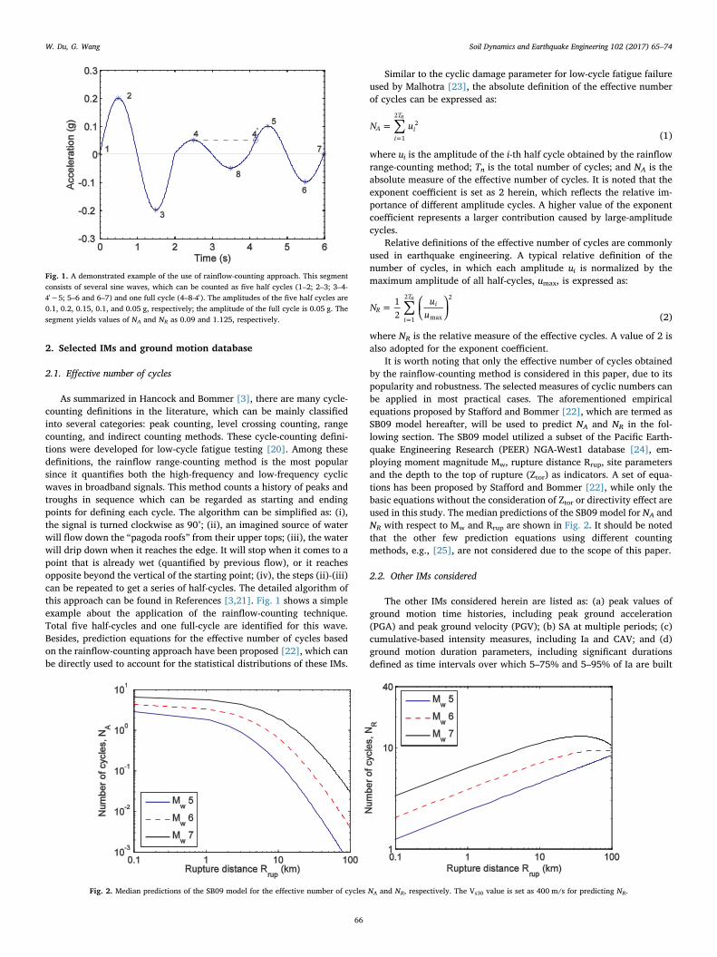
It is worth noting that only the effective number of cycles obtainedby the rainflow-counting method is considered in this paper, due to itspopularity and robustness. The selected measures of cyclic numbers canbe applied in most practical cases. The aforementioned empiricalequations proposed by Stafford and Bommer [22], which are termed asSB09 model hereafter, will be used to predict NA and NR in the fol-lowing section. The SB09 model utilized a subset of the Pacific Earth-quake Engineering Research (PEER) NGA-West1 database [24], em-ploying moment magnitude Mw, rupture distance Rrup, site parametersand the depth to the top of rupture (Ztor) as indicators. A set of equa-tions has been proposed by Stafford and Bommer [22], while only thebasic equations without the consideration of Ztor or directivity effect areused in this study. The median predictions of the SB09 model for NA andNR with respect to Mw and Rrup are shown in Fig. 2. It should be notedthat the other few prediction equations using different countingmethods, e.g., [25], are not considered due to the scope of this paper.

2.2. Other IMs considered

The other IMs considered herein are listed as: (a) peak values ofground motion time histories, including peak ground acceleration(PGA) and peak ground velocity (PGV); (b) SA at multiple periods; (c)cumulative-based intensity measures, including Ia and CAV; and (d)ground motion duration parameters, including significant durationsdefined as time intervals over which 5–75% and 5–95% of Ia are built

Fig. 1. A demonstrated example of the use of rainflow-counting approach. This segmentconsists of several sine waves, which can be counted as five half cycles (1–2; 2–3; 3–4-′4 −5; 5–6 and 6–7) and one full cycle (4–8- ′4 ). The amplitudes of the five half cycles are0.1, 0.2, 0.15, 0.1, and 0.05 g, respectively; the amplitude of the full cycle is 0.05 g. Thesegment yields values of NA and NR as 0.09 and 1.125, respectively.

Fig. 2. Median predictions of the SB09 model for the effective number of cycles NA and NR, respectively. The Vs30 value is set as 400 m/s for predicting NR.

W. Du, G. Wang Soil Dynamics and Earthquake Engineering 102 (2017) 65–74

66

up (termed as Ds5–75 and Ds5–95, respectively). The selected IMs cover arange of amplitude-, intensity-, and duration-based parameters, re-presenting various characteristics of earthquake loadings. The IMsconsidered as well as their definitions are summarized in Table 1.

Several GMPEs are needed to predict the statistical distributions(medians and standard deviations) of these IMs. For PGA, PGV, and SA,since the SB09 model for NA and NR was developed using the NGA-West1 database, it seems not necessary to select the recently proposedNGA-West2 GMPEs. Instead, the GMPEs of the NGA-West1 project forshallow crustal earthquakes in active tectonic regions are adopted:Abrahamson and Silva [26], Boore and Atkinson [27], Campbell andBozorgnia [28], and Chiou and Youngs [29]. They are referred to asAS08, BA08, CB08, and CY08, respectively. The GMPEs proposed byTravasarou and Bray [30], Foulser-Piggott and Stafford [31], andCampbell and Bozorgnia [32] are chosen to estimate the statisticaldistribution of Ia. For CAV, only two GMPEs [33,34] were developedusing the global ground motion database, so they are adopted.

The GMPEs proposed by Kempton and Stewart [35] (KS06),Bommer et al. [36] (BSA09), and Du and Wang [37] (DW17) are usedfor predicting the significant durations Ds5–75 and Ds5–95. The KS06model was developed based on the analysis of magnitude effects onsource duration, while the BSA09 and DW17 models were empiricallyderived using subsets of the NGA database. Only the base function(without the consideration of fault type or directivity effect) of the KS06model is used herein. All the selected GMPEs as well as their ab-breviations are also summarized in Table 1.

2.3. Ground motion database

A subset of the NGA database is selected to calculate the empiricalvalues of the IMs considered. The ground motion database selected isalmost identical to that used in deriving the CB08 model [28], including1560 recordings from 64 earthquakes with moment magnitudes from4.3 to 7.9 and rupture distances from 0.1 to 199 km. The completerecording list regarding the database can be found in Campbell andBozorgnia [38]. Fig. 3(a) shows the distribution of moment magnitudeand rupture distance contained in the database.

It should be noted that each recorded time history has a usableperiod range, in order to eliminate low-frequency or high-frequencynoises. Therefore, SA at periods larger than the maximum usable periodshould not be used for subsequent correlation analyses. The number ofusable ground motions is expected to decrease as vibration period in-creases, as is shown in Fig. 3(b).

3. Empirical correlation analyses

3.1. Computational procedures for correlation coefficients

Current GMPEs usually assume that IMs are logarithmically nor-mally distributed, which can be shown as:

= + +IM IM η εln( ) ln( )i i i i (3)

where IMln( )i and IMln( )i denote the measured (geometric mean of twohorizontal components of each record) and the predicted logarithmic i-th IM (e.g., SA, Ia, NA), respectively. ηi and εi represent the inter-eventand intra-event residuals of the i-th IM (normally distributed with zerosmeans and standard deviations τ and σ), respectively. The total standarddeviation σT is given as = +σ τ σT

2 2 2 . The values of τ, σ, and σT forvarious IMs are generally provided by GMPEs.

The Pearson product-moment correlation coefficient is a widelyused measure of linear correlation between two variables [39]. Thecorrelation coefficients between the inter-event or intra-event residualsof different IMs can be estimated as:

=∑ − −

∑ − ∑ −=

= =

ρx x x x

x x x x

( )( )

( ) ( )x x

in i i

in i

jn j

1 1( )

1 2( )

2

1 1( )

12

1 2( )

221, 2

(4)

where x1 and x2 are random variables (e.g., η1 and η2 for the inter-event residuals of IM1 and IM2); n is the total number of the randomvariables considered (i.e., number of earthquakes for the inter-eventcorrelation, or number of ground motion records for the intra-eventcorrelation); and x1 and x2 denote the sample mean of variables x1and x2, respectively. In this paper, IM1 refers to NA or NR, and IM2

refers to the other aforementioned measures such as PGA, SA, and Ia.For each pair of IMs, ρη η1, 2

and ρε ε1, 2 can be computed via Eq. (4).Under the assumption that ηi and εi are independent [40], the

correlation between the total residuals can be expressed as:

=⋅

+( )ρσ σ

ρ τ τ ρ σ σ1ε ε

T Tη η ε ε1 2 1 2T T1, 2

1 21, 2 1, 2 (5)

where τk, σk, and σTk (k = 1, 2) are the standard deviations of the inter-event, intra-event, and total residuals for the k-th IM, respectively.Thus, the correlation between the total residuals for each pair of IMscan be calculated via Eqs. (4) and (5) accordingly.

The above statistical analysis only provides the point-estimate of thecorrelation coefficient, while the uncertainty of ρ should also be ac-counted for carefully. Such uncertainty is due to the finite number ofsample size, as well as different ground motion models used in its de-termination. A bootstrap method is often used to construct the con-fidence intervals of correlation coefficients [39]. The basic idea of thismethod is to re-sample the observed dataset by random sampling withreplacement from the original dataset, and then the correlation coeffi-cients of these bootstrap replicates can be calculated. This process needsto be repeated a certain number of times to accurately estimate thevariance of ρ.

In addition to the bootstrap method, another widely used method isthe Fisher z transformation [41]. This method converts the correlationcoefficient ρ into a transformed variable z via:

⎜ ⎟= ⎛⎝

+−

⎞⎠

= −zρρ

ρ12

ln11

tanh 1

(6)

where ρ is the Pearson correlation coefficient; −tanh 1 is the inverse

Table 1Summary of the IMs considered in this study.

IM parameters Definition* GMPEs used

Abbreviations Reference

NA Shown in Eq. (1) SB09 Stafford andBommer [22]NR Shown in Eq. (2)

PGA a tmax( ( ) ) AS08 Abrahamson andSilva [26]

BA08 Boore and Atkinson[27]

PGV v tmax( ( ) ) CB08 Campbell andBozorgnia [28]

SA(T) Peak response of a linearelastic system

CY08 Chiou and Youngs[29]

Ia ∫ a t dt( )πg

t2 0

max 2 [44] TBA03 Travasarou et al.[30]

FS12 Foulser-Piggott andStafford [31]

CB12 Campbell andBozorgnia [32]

CAV ∫ a t dt( )t0

max [45] CB10 Campbell andBozorgnia [33]

DW13 Du and Wang [34]Ds5-75 Time interval between

5% to 75% of IaKS06 Kempton and

Stewart [35]BSA09 Bommer et al. [36]Ds5-95 Time interval between

5% to 95% of Ia DW17 Du and Wang [37]

* a(t): Acceleration-time history; v(t):velocity-time history; tmax: total duration of theground motion time history and g is gravitational acceleration.

W. Du, G. Wang Soil Dynamics and Earthquake Engineering 102 (2017) 65–74

67

hyperbolic tangent function; and z is the transformed correlationcoefficient which is approximately normally distributed. The varianceof ρ usually becomes smaller when it approaches 1 or −1, whereas thevariance of the transformed variable z can keep approximately constantfor all ρ values. Therefore, if the mean and standard deviation of thetransformed variable z are denoted as μz and σz, respectively, the cor-responding median correlation coefficient ρ50 can be computed as:

⎜ ⎟= ⎛⎝

−+

⎞⎠

=ρ ee

μ11

tanh( )μ

μ z50

2

2

z

z (7)

Similarly, a certain percentile of ρ can be obtained using μz and σz

(e.g., = +ρ μ σtanh( )z z84 ; = −ρ μ σtanh( )z z16 ).

3.2. Correlations of cyclic numbers with PGA, PGV, and SA

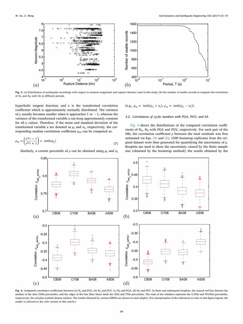
Fig. 4 shows the distributions of the computed correlation coeffi-cients of NA, NR with PGA and PGV, respectively. For each pair of theIMs, the correlation coefficient ρ between the total residuals was firstestimated via Eqs. (4) and (5); 1500 bootstrap replicates from the ori-ginal dataset were then generated for quantifying the uncertainty of ρ.Boxplots are used to show the uncertainty caused by the finite samplesize (obtained by the bootstrap method); the results obtained by the

(a) (b)

Fig. 3. (a) Distribution of earthquake recordings with respect to moment magnitude and rupture distance used in this study; (b) the number of usable records to compute the correlationof NA and NR with SA at different periods.

(a) (b)

(c) (d)

Fig. 4. Computed correlation coefficients between (a) NA and PGA, (b) NA and PGV, (c) NR and PGA, (d) NR and PGV. In these and subsequent boxplots, the central red line denotes themedian of the data (50th percentile), and the edges of the box (blue lines) mark the 25th and 75th percentiles. The ends of the whiskers represent the 0.35th and 99.65th percentiles,respectively; the red plus symbols denote outliers. The results obtained by various GMPEs are shown in each subplot. (For interpretation of the references to color in this figure legend, thereader is referred to the web version of this article.)

W. Du, G. Wang Soil Dynamics and Earthquake Engineering 102 (2017) 65–74

68

four aforementioned GMPEs are shown in each boxplot. Fig. 4(a) and(b) illustrate that the correlations of NA with PGA and PGV are positivewith median values of approximately 0.78 and 0.4, respectively. This isnot surprising, since NA represents the summation of the amplitude foreach half cycle, which is expected to be larger if PGA of a groundmotion is higher. Fig. 4(c) and (d) show the computed correlations ofNR with PGA and PGV, respectively. Unlike the case of NA, the corre-lations of NR-PGA and NR-PGV are generally negative, with medianvalues of approximately −0.36 and −0.46, respectively. Hence, as arelative definition, NR has a much weaker correlation with PGA com-pared with NA because of the normalization process. For PGV, NR ex-hibits slightly stronger correlation than NA, although the NR-PGV cor-relation is found to be negative. Besides, it can also be seen that theuncertainty (i.e., 25th and 75th percentiles represented by the edges ofthe box) due to the finite sample size is generally in the range of0.02–0.03, whereas the variability from the use of different GMPEs ismore notable. There appears to be no specific GMPE which yields sys-tematically higher or lower correlations. The results (a number of ρbased on the bootstrap method) obtained by various GMPEs werecombined together in a logic-tree framework with equal weight as-signed. The combined results were then transformed via Eq. (6) toevaluate μz and σz. The calculated median correlation coefficients ρ50, aswell as σz are listed in Table 2.

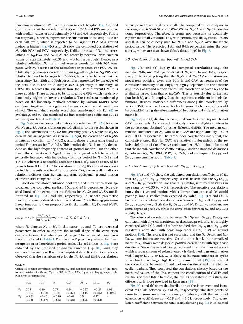
Fig. 5 shows the computed empirical correlations [Eq. (5)] betweenNA, NR and SA versus vibration period. Similar to the results shown inFig. 4, the correlations of NA-SA are generally positive, while the NR-SAcorrelations are negative. As seen in Fig. 5(a), the correlation of NA-SAis generally constant for T<0.2 s, and it shows a decreasing trend asperiod T increases for T>0.2 s. This implies that NA is mainly depen-dent on the high-frequency content of ground motions. On the otherhand, the correlation of NR-SA is in the range of −0.4 to −0.1. Itgenerally increases with increasing vibration period for T< 0.1 s andT>1 s, whereas a noticeable decreasing trend of ρ can be observed forperiods from 0.1 s to 1 s. The variation of the NR-SA correlation versusperiod is presently not feasible to explain. Yet, the overall small cor-relation indicates that NR can represent additional ground motioncharacteristics compared to SA.

Based on the aforementioned bootstrap and z transformation ap-proaches, the computed median, 16th and 84th percentiles (blue da-shed lines) of the correlation coefficients for NA-SA and NR-SA are il-lustrated in Fig. 6(a) and (b), respectively. A smooth parametricfunction is usually desirable for practical use. The following piecewiselinear function is then proposed to fit the median NA-SA and NR-SAcorrelations:

= + − ≤ ≤+

+ +ρ a T TT T

a a T T Tln( / )ln( / )

( )nn

n nn n n nNx,SA

11 1

(8)

where Nx denotes NA or NR in this paper; an and Tn are regressedparameters in order to capture the overall shape of the correlationcoefficients over the whole period range. The values of these para-meters are listed in Table 3. For any give T, ρ can be predicted by linearinterpolation in logarithmic period scale. The solid lines in Fig. 6 areobtained by the proposed parametric function [Eq. (8)], and theycompare reasonably well with the empirical data. Besides, it can also beobserved that the variations of ρ for the NA-SA and NR-SA correlations

versus period T are relatively small. The computed values of σz are inthe ranges of 0.03–0.07 and 0.03–0.05 for NA-SA and NR-SA correla-tions, respectively. Therefore, it seems not necessary to accuratelycapture the small variations of σz with periods, and the σz values of 0.05and 0.04 can be directly used for NA-SA and NR-SA over the wholeperiod range. The predicted 16th and 84th percentiles using the con-stant σz values are also shown (black dotted line) in Fig. 6.

3.3. Correlation of cyclic numbers with Ia and CAV

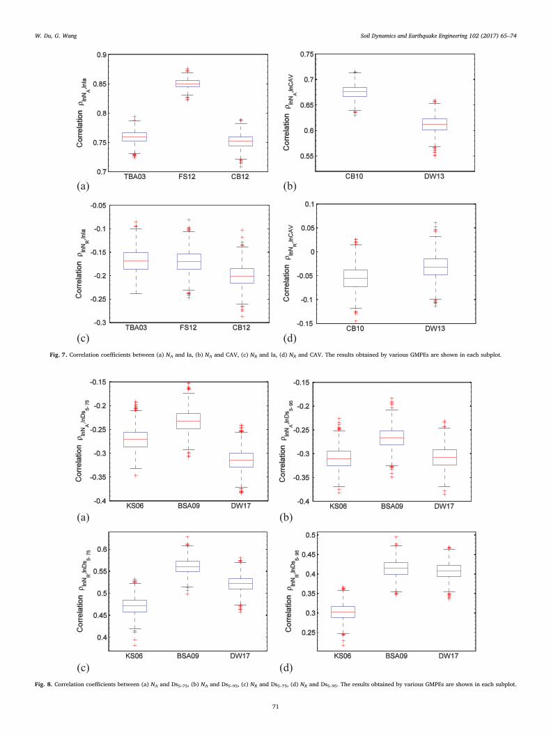
Fig. 7(a) and (b) display the computed correlations (e.g., themedian, 25th, and 75th percentiles) of NA with Ia and CAV, respec-tively. It is not surprising that the NA-Ia and NA-CAV correlations aremoderately positive, given that both Ia and CAV, as measures of thecumulative intensity of shakings, are highly dependent on the absoluteamplitudes of ground motion cycles. The correlation between NA and Iais slightly larger than that of NA-CAV. This is possibly due to the factthat both NA and Ia employ 2 as the exponent coefficient in their de-finitions. Besides, noticeable differences among the correlations byvarious GMPEs can be observed for both figures. Such uncertainty couldbe quantified using the aforementioned bootstrap and z transformationmethods.

Fig. 7(c) and (d) display the computed correlations of NR with Ia andCAV, respectively. As observed previously, there are slight variations inthe correlations obtained by using different GMPEs. The median cor-relation coefficients of NR with Ia and CAV are approximately −0.19and −0.04, respectively. The rather poor correlations imply that, thecumulative-based IMs (Ia, CAV) are relatively independent of the re-lative definition of the effective cyclic number (NR). It should be notedthat the median correlation coefficients ρ50, and the standard deviationsσz between NA, NR, PGA, PGV, Ia, CAV, and subsequent Ds5–75 andDs5–95, are summarized in Table 2.

3.4. Correlation of cyclic numbers with Ds5-75 and Ds5-95

Fig. 8(a) and (b) show the calculated correlation coefficients of NA

with Ds5–75 and Ds5–95, respectively. It can be seen that the NA-Ds5–75and NA-Ds5–95 correlations are generally similar, with median values inthe range of −0.35 to −0.2, respectively. The negative correlationsimply that a ground motion with a longer than expected Ds wouldpossibly have a smaller than expected NA value. Fig. 8(c) and (d) il-lustrate the calculated correlation coefficients of NR with Ds5–75 andDs5–95, respectively. Both the NR-Ds5–75 and NR-Ds5–95 correlations aresome degree of positive, while the correlation between NR and Ds5–75 isslightly larger.

The observed correlations between NA, NR and Ds5–75, Ds5–95 areconsistent with physical intuitions. As discussed previously, NA is highlycorrelated with PGA, and it has been studied that Ds5–75 and Ds5–95 arenegatively correlated with peak amplitudes (PGA, PGV) of groundmotions [14]. Therefore, it is not surprising that the NA-Ds5–75 and NA-Ds5–95 correlations are negative. On the other hand, the normalizedmeasure NR shows some degree of positive correlations with significantdurations. Since Ds5–75 and Ds5–95 represent the time interval acrosswhich a great amount of seismic energy is dissipated, a ground motionwith longer Ds5–75 or Ds5–95 is likely to be more numbers of cyclicwaves (and hence larger NR). Besides, Bommer et al. [19] also studiedthe correlations between ground motion durations and the effectivecyclic numbers. They computed the correlations directly based on themeasured values of the IMs, without the consideration of GMPEs andresiduals of these IMs. Therefore, the results presented in this study aredifferent with those provided in Reference [19].

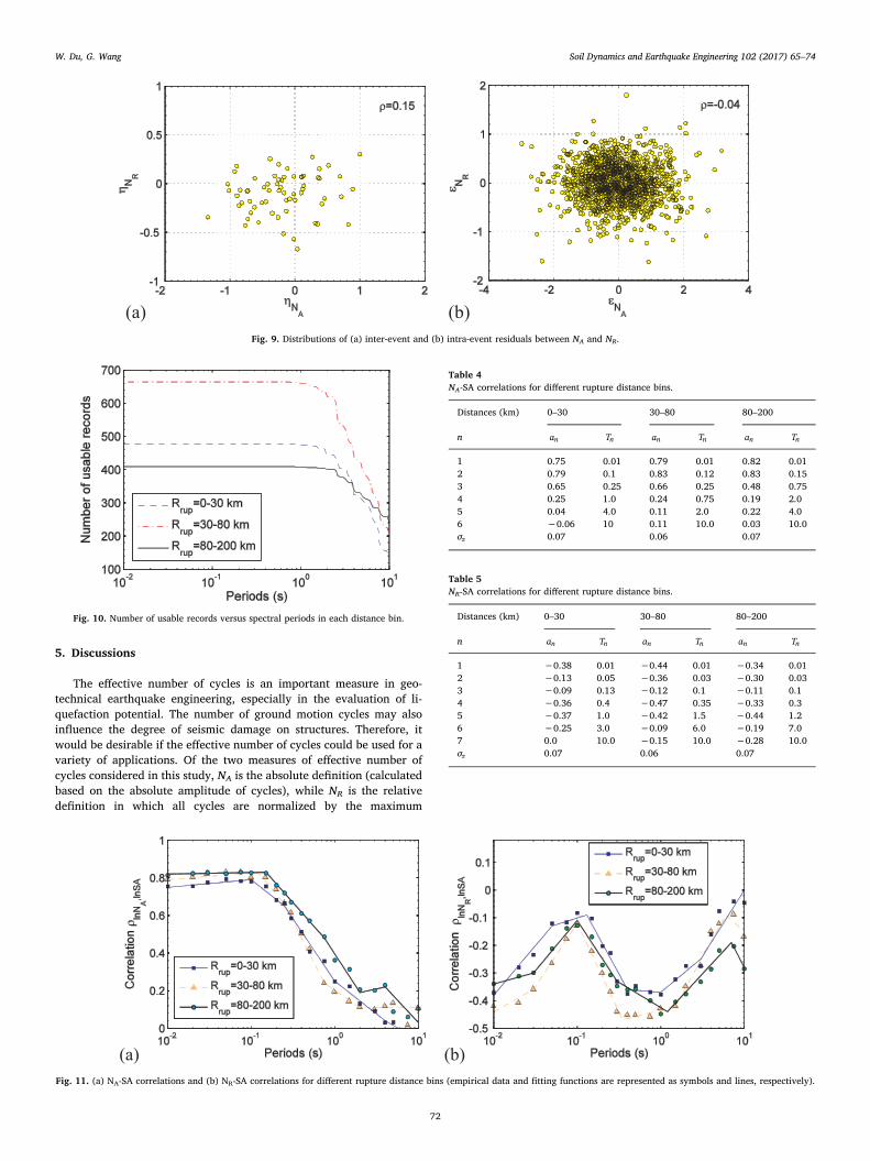
Fig. 9(a) and (b) show the distribution of the inter-event and intra-event residuals between NA and NR, respectively. The data points ofthese two figures are almost randomly distributed, with the computedcorrelation coefficients as +0.15 and −0.04, respectively. The corre-lation coefficient between the total residuals using Eq. (5) is calculated

Table 2Computed median correlation coefficients ρ50 and standard deviations σz of the trans-formed variable z for NA and NR with PGA, PGV, Ia, CAV, Ds5–75, and Ds5–95, respectively.σz is given in parentheses.

PGA PGV Ia CAV Ds5-75 Ds5-95 NR

NA 0.78(0.057)

0.40(0.043)

0.79(0.13)

0.64(0.061)

−0.27(0.045)

−0.29(0.035)

0.03(0.025)

NR −0.35(0.046)

−0.46(0.057)

−0.19(0.032)

−0.04(0.029)

0.51(0.056)

0.37(0.064)

–

W. Du, G. Wang Soil Dynamics and Earthquake Engineering 102 (2017) 65–74

69

as 0.03. Such poor correlation indicates that, although both NA and NR

represent the effective numbers of cycles of a ground motion, thephysical interpretations of these two measures are significantly dif-ferent. Therefore, NA and NR are better suited for different applications.

4. Influence of rupture distance on NA-SA and NR-SA correlations

It is tempting to examine the influence of causal parameters (i.e.,Mw, Rrup) on the NA-SA and NR-SA correlations. The influence of mag-nitude Mw on the correlations is found to be less significant than Rrup.Therefore, only the influence of rupture distance on the correlations isinvestigated in this section.

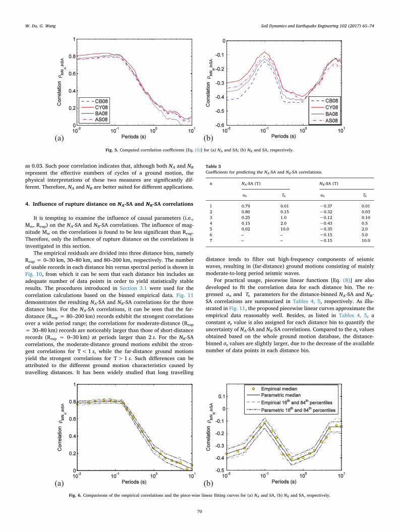
The empirical residuals are divided into three distance bins, namelyRrup = 0–30 km, 30–80 km, and 80–200 km, respectively. The numberof usable records in each distance bin versus spectral period is shown inFig. 10, from which it can be seen that each distance bin includes anadequate number of data points in order to yield statistically stableresults. The procedures introduced in Section 3.1 were used for thecorrelation calculations based on the binned empirical data. Fig. 11demonstrates the resulting NA-SA and NR-SA correlations for the threedistance bins. For the NA-SA correlations, it can be seen that the far-distance (Rrup = 80–200 km) records exhibit the strongest correlationsover a wide period range; the correlations for moderate-distance (Rrup

= 30–80 km) records are noticeably larger than those of short-distancerecords (Rrup = 0–30 km) at periods larger than 2 s. For the NR-SAcorrelations, the moderate-distance ground motions exhibit the stron-gest correlations for T< 1 s, while the far-distance ground motionsyield the strongest correlations for T> 1 s. Such differences can beattributed to the different ground motion characteristics caused bytravelling distances. It has been widely studied that long travelling

distance tends to filter out high-frequency components of seismicwaves, resulting in (far-distance) ground motions consisting of mainlymoderate-to-long period seismic waves.

For practical usage, piecewise linear functions [Eq. (8)] are alsodeveloped to fit the correlation data for each distance bin. The re-gressed an and Tn parameters for the distance-binned NA-SA and NR-SA correlations are summarized in Tables 4, 5, respectively. As illu-strated in Fig. 11, the proposed piecewise linear curves approximate theempirical data reasonably well. Besides, as listed in Tables 4, 5, aconstant σz value is also assigned for each distance bin to quantify theuncertainty of NA-SA and NR-SA correlations. Compared to the σz valuesobtained based on the whole ground motion database, the distance-binned σz values are slightly larger, due to the decrease of the availablenumber of data points in each distance bin.

(a) (b)

Fig. 5. Computed correlation coefficients [Eq. (5)] for (a) NA and SA; (b) NR and SA, respectively.

(a) (b)

Fig. 6. Comparisons of the empirical correlations and the piece-wise linear fitting curves for (a) NA and SA, (b) NR and SA, respectively.

Table 3Coefficients for predicting the NA-SA and NR-SA correlations.

n NA-SA (T) NR-SA (T)

an Tn an Tn

1 0.79 0.01 −0.37 0.012 0.80 0.15 −0.32 0.033 0.25 1.0 −0.12 0.104 0.15 2.0 −0.43 0.55 0.02 10.0 −0.35 2.06 – – −0.15 5.07 – – −0.15 10.0

W. Du, G. Wang Soil Dynamics and Earthquake Engineering 102 (2017) 65–74

70

(a) (b)

(c) (d)

Fig. 7. Correlation coefficients between (a) NA and Ia, (b) NA and CAV, (c) NR and Ia, (d) NR and CAV. The results obtained by various GMPEs are shown in each subplot.

(a) (b)

(c) (d)

Fig. 8. Correlation coefficients between (a) NA and Ds5–75, (b) NA and Ds5–95, (c) NR and Ds5–75, (d) NR and Ds5–95. The results obtained by various GMPEs are shown in each subplot.

W. Du, G. Wang Soil Dynamics and Earthquake Engineering 102 (2017) 65–74

71

5. Discussions

The effective number of cycles is an important measure in geo-technical earthquake engineering, especially in the evaluation of li-quefaction potential. The number of ground motion cycles may alsoinfluence the degree of seismic damage on structures. Therefore, itwould be desirable if the effective number of cycles could be used for avariety of applications. Of the two measures of effective number ofcycles considered in this study, NA is the absolute definition (calculatedbased on the absolute amplitude of cycles), while NR is the relativedefinition in which all cycles are normalized by the maximum

(a) (b)

Fig. 9. Distributions of (a) inter-event and (b) intra-event residuals between NA and NR.

Fig. 10. Number of usable records versus spectral periods in each distance bin.

(a) (b)

Fig. 11. (a) NA-SA correlations and (b) NR-SA correlations for different rupture distance bins (empirical data and fitting functions are represented as symbols and lines, respectively).

Table 4NA-SA correlations for different rupture distance bins.

Distances (km) 0–30 30–80 80–200

n an Tn an Tn an Tn

1 0.75 0.01 0.79 0.01 0.82 0.012 0.79 0.1 0.83 0.12 0.83 0.153 0.65 0.25 0.66 0.25 0.48 0.754 0.25 1.0 0.24 0.75 0.19 2.05 0.04 4.0 0.11 2.0 0.22 4.06 −0.06 10 0.11 10.0 0.03 10.0σz 0.07 0.06 0.07

Table 5NR-SA correlations for different rupture distance bins.

Distances (km) 0–30 30–80 80–200

n an Tn an Tn an Tn

1 −0.38 0.01 −0.44 0.01 −0.34 0.012 −0.13 0.05 −0.36 0.03 −0.30 0.033 −0.09 0.13 −0.12 0.1 −0.11 0.14 −0.36 0.4 −0.47 0.35 −0.33 0.35 −0.37 1.0 −0.42 1.5 −0.44 1.26 −0.25 3.0 −0.09 6.0 −0.19 7.07 0.0 10.0 −0.15 10.0 −0.28 10.0σz 0.07 0.06 0.07

W. Du, G. Wang Soil Dynamics and Earthquake Engineering 102 (2017) 65–74

72

amplitude of cycles. It has been found that NA is highly correlated withhigh-frequency IMs such as PGA, Ia, and SA at short periods. Comparedto PGA, NA considers not only the effect of the single cycle with peakamplitude, but also the effect of a number of secondary cycles. Hence,NA can be regarded as a surrogate of PGA in some cases, in which theestimation of cyclic deformation demand is important [42]. In contrast,NR exhibits small-to-moderate negative correlations with PGA, PGV, Ia,and SA, indicating that NR can provide some supplementary informa-tion regarding the ground motion characteristics compared with theseIMs. Therefore, although NR alone may not be very useful, NR in con-junction with primary IMs (e.g., PGA, SA) would be favorable in someengineering applications.

It is not surprising that NA, as an amplitude-based indicator, exhibitsnegative correlations with Ds5–75 and Ds5–95. The correlations of NR

with Ds5–75 and Ds5–95 are just moderately positive (with maximum ρ50as 0.51), which may contradict the assumption that duration measurescan effectively represent the number of cycles of ground motions. Theseresults are some degree of consistent with a previous study which statedthat the correlations between ground motion durations and the numberof effective cycles are weak [19].

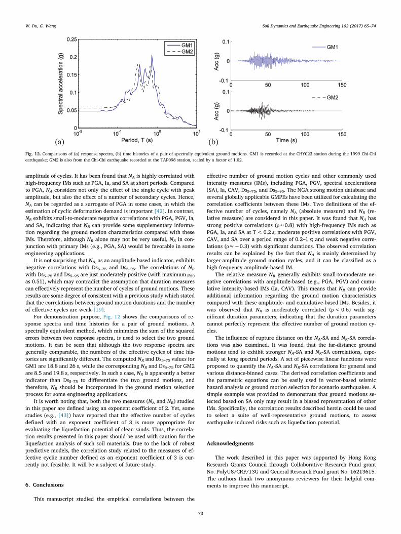
For demonstration purpose, Fig. 12 shows the comparisons of re-sponse spectra and time histories for a pair of ground motions. Aspectrally equivalent method, which minimizes the sum of the squarederrors between two response spectra, is used to select the two groundmotions. It can be seen that although the two response spectra aregenerally comparable, the numbers of the effective cycles of time his-tories are significantly different. The computed NR and Ds5–75 values forGM1 are 18.8 and 26 s, while the corresponding NR and Ds5–75 for GM2are 8.5 and 19.8 s, respectively. In such a case, NR is apparently a betterindicator than Ds5–75 to differentiate the two ground motions, andtherefore, NR should be incorporated in the ground motion selectionprocess for some engineering applications.

It is worth noting that, both the two measures (NA and NR) studiedin this paper are defined using an exponent coefficient of 2. Yet, somestudies (e.g., [43]) have reported that the effective number of cyclesdefined with an exponent coefficient of 3 is more appropriate forevaluating the liquefaction potential of clean sands. Thus, the correla-tion results presented in this paper should be used with caution for theliquefaction analysis of such soil materials. Due to the lack of robustpredictive models, the correlation study related to the measures of ef-fective cyclic number defined as an exponent coefficient of 3 is cur-rently not feasible. It will be a subject of future study.

6. Conclusions

This manuscript studied the empirical correlations between the

effective number of ground motion cycles and other commonly usedintensity measures (IMs), including PGA, PGV, spectral accelerations(SA), Ia, CAV, Ds5–75, and Ds5–95. The NGA strong motion database andseveral globally applicable GMPEs have been utilized for calculating thecorrelation coefficients between these IMs. Two definitions of the ef-fective number of cycles, namely NA (absolute measure) and NR (re-lative measure) are considered in this paper. It was found that NA hasstrong positive correlations (ρ≈0.8) with high-frequency IMs such asPGA, Ia, and SA at T<0.2 s; moderate positive correlations with PGV,CAV, and SA over a period range of 0.2–1 s; and weak negative corre-lations (ρ≈−0.3) with significant durations. The observed correlationresults can be explained by the fact that NA is mainly determined bylarger-amplitude ground motion cycles, and it can be classified as ahigh-frequency amplitude-based IM.

The relative measure NR generally exhibits small-to-moderate ne-gative correlations with amplitude-based (e.g., PGA, PGV) and cumu-lative intensity-based IMs (Ia, CAV). This means that NR can provideadditional information regarding the ground motion characteristicscompared with these amplitude- and cumulative-based IMs. Besides, itwas observed that NR is moderately correlated (ρ<0.6) with sig-nificant duration parameters, indicating that the duration parameterscannot perfectly represent the effective number of ground motion cy-cles.

The influence of rupture distance on the NA-SA and NR-SA correla-tions was also examined. It was found that the far-distance groundmotions tend to exhibit stronger NA-SA and NR-SA correlations, espe-cially at long spectral periods. A set of piecewise linear functions wereproposed to quantify the NA-SA and NR-SA correlations for general andvarious distance-binned cases. The derived correlation coefficients andthe parametric equations can be easily used in vector-based seismichazard analysis or ground motion selection for scenario earthquakes. Asimple example was provided to demonstrate that ground motions se-lected based on SA only may result in a biased representation of otherIMs. Specifically, the correlation results described herein could be usedto select a suite of well-representative ground motions, to assessearthquake-induced risks such as liquefaction potential.

Acknowledgments

The work described in this paper was supported by Hong KongResearch Grants Council through Collaborative Research Fund grantNo. PolyU8/CRF/13G and General Research Fund grant No. 16213615.The authors thank two anonymous reviewers for their helpful com-ments to improve this manuscript.

(a) (b)

Fig. 12. Comparisons of (a) response spectra, (b) time histories of a pair of spectrally equivalent ground motions. GM1 is recorded at the CHY023 station during the 1999 Chi-Chiearthquake; GM2 is also from the Chi-Chi earthquake recorded at the TAP098 station, scaled by a factor of 1.02.

W. Du, G. Wang Soil Dynamics and Earthquake Engineering 102 (2017) 65–74

73

References

[1] Seed HB, Lee KL. Liquefaction of saturated sands during cyclic loading. J Soil MechFound Div 1966;92(6):105–34.

[2] Martin GR, Finn WL, Seed HB. Fundementals of liquefaction under cyclic loading. JGeotech Geoenviron Eng (ASCE) 1975. [101(ASCE# 11231 Proceeding)].

[3] Hancock J, Bommer JJ. The effective number of cycles of earthquake ground mo-tion. Earthq Eng Struct Dyn 2005;34(6):637–64.

[4] Annaki M, Lee KL. Equivalent uniform cycle concept for soil dynamics. J GeotechEng Div (ASCE) 1977;103(6):549–64.

[5] Kramer SL. Geotechnical earthquake engineering. New Jersey: Practice Hall; 1996.p. 653.

[6] Green RA, Terri GA. Number of equivalent cycles concept for liquefactionevaluations—Revisited. J Geotech Geoenviron Eng 2005;131(4):477–88.

[7] Rathje EM, Saygili G. Probabilistic seismic hazard analysis for the sliding dis-placement of slopes: scalar and vector approaches. J Geotech Geoenviron Eng2008;134(6):804–14.

[8] Du W, Wang G. Fully probabilistic seismic displacement analysis of spatially dis-tributed slopes using spatially correlated vector intensity measures. Earthq EngStruct Dyn 2014;43(5):661–79.

[9] Baker JW, Cornell AC. A vector-valued ground motion intensity measure consistingof spectral acceleration and epsilon. Earthq Eng Struct Dyn 2005;34(10):1193–217.

[10] Wang G. A ground motion selection and modification method capturing responsespectrum characteristics and variability of scenario earthquakes. Soil Dyn EarthqEng 2011;31(4):611–25.

[11] Jayaram N, Lin T, Baker JW. A computationally efficient ground-motion selectionalgorithm for matching a target response spectrum mean and variance. EarthqSpectra 2011;27(3):797–815.

[12] Bradley BA. A ground motion selection algorithm based on the generalized condi-tional intensity measure approach. Soil Dyn Earthq Eng 2012;40:48–61.

[13] Baker JW, Jayaram N. Correlation of spectral acceleration values from NGA groundmotion models. Earthq Spectra 2008;24(1):299–317.

[14] Bradley BA. Correlation of significant duration with amplitude and cumulative in-tensity measures and its use in ground motion selection. J Earthq Eng2011;15(6):809–32.

[15] Bradley BA. Empirical correlations between peak ground velocity and spectrum-based intensity measures. Earthq Spectra 2012;28(1):17–35.

[16] Bradley BA. Correlation of arias intensity with amplitude, duration and cumulativeintensity measures. Soil Dyn Earthq Eng 2015;78:89–98.

[17] Wang G, Du W. Empirical correlations between cumulative absolute velocity andspectral accelerations from NGA ground motion database. Soil Dyn Earthq Eng2012;43:229–36.

[18] Du W. Empirical correlations of frequency content parameters of ground motionswith other intensity measures. J Earthq Eng 2017. http://dx.doi.org/10.1080/13632469.2017.1342303. (published online).

[19] Bommer JJ, Hancock J, Alarcón JE. Correlations between duration and number ofeffective cycles of earthquake ground motion. Soil Dyn Earthq Eng2006;26(1):1–13.

[20] Dowling NE. Fatigue failure predictions for complicated stress-strain histories. JMater 1972;7(1):71–87.

[21] Amzallag C, Gerey JP, Robert JL, Bahuaud J. Standardization of the rainflowcounting method for fatigue analysis. Int J Fatigue 1994;16(4):287–93.

[22] Stafford PJ, Bommer JJ. Empirical equations for the prediction of the equivalentnumber of cycles of earthquake ground motion. Soil Dyn Earthq Eng2009;29(11):1425–36.

[23] Malhotra PK. Cyclic-demand spectrum. Earthq Eng Struct Dyn 2002;31(7):1441–57.

[24] Chiou B, Darragh R, Gregor N, Silva W. NGA project strong-motion database. EarthqSpectra 2008;24(1):23–44.

[25] Liu AH, Stewart JP, Abrahamson NA, Moriwaki Y. Equivalent number of uniformstress cycles for soil liquefaction analysis. J Geotech Geoenviron Eng2001;127(12):1017–26.

[26] Abrahamson NA, Silva WJ. Summary of the Abrahamson & Silva NGA ground-mo-tion relations. Earthq Spectra 2008;24(1):67–97.

[27] Boore DM, Atkinson GM. Ground-motion prediction equations for the averagehorizontal component of PGA, PGV and 5%-damped PSA at spectral periods be-tween 0.01s and 10 s. Earthq Spectra 2008;24(1):99–138.

[28] Campbell KW, Bozorgnia Y. NGA ground motion model for the geometric meanhorizontal component of PGA, PGV, PGD and 5% damped linear elastic responsespectra for periods ranging from 0.1 to 10 s. Earthq Spectra 2008;24(1):139–71.

[29] Chiou BJ, Youngs RR. An NGA model for the average horizontal component of peakground motion and response spectra. Earthq Spectra 2008;24(1):173–215.

[30] Travasarou T, Bray JD. Empirical attenuation relationship for Arias Intensity.Earthq Eng Struct Dyn 2003;32(7):1133–55.

[31] Foulser-Piggott RF, Stafford PJ. A predictive model for Arias intensity at multiplesites and consideration of spatial correlations. Earthq Eng Struct Dyn2012;41(3):431–51.

[32] Campbell KW, Bozorgnia Y. A comparison of ground motion prediction equationsfor Arias intensity and cumulative absolute velocity developed using a consistentdatabase and functional form. Earthq Spectra 2012;28(3):931–41.

[33] Campbell KW, Bozorgnia Y. A ground motion prediction equation for the horizontalcomponent of cumulative absolute velocity (CAV) based on the PEER-NGA strongmotion database. Earthq Spectra 2010;26(3):635–50.

[34] Du W, Wang G. A simple ground-motion prediction model for cumulative absolutevelocity and model validation. Earthq Eng Struct Dyn 2013;42(8):1189–202.

[35] Kempton JJ, Stewart JP. Prediction equations for significant duration of earthquakeground motions considering site and near-source effects. Earthq Spectra2006;22(4):985–1013.

[36] Bommer JJ, Stafford PJ, Alarcón JE. Empirical equations for the prediction of thesignificant, bracketed, and uniform duration of earthquake ground motion. BullSeismol Soc Am 2009;99(6):3217–33.

[37] Du W, Wang G. Prediction equations for ground-motion significant durations usingthe NGA-West2 database. Bull Seismol Soc Am 2017;107(1):319–33.

[38] Campbell KW, Bozorgnia Y. Campbell-Bozorgnia NGA ground motion relations forthe geometric mean horizontal component of peak and spectral ground motionparameters. Berkeley: Pacific Earthquake Engineering Research Center, Universityof California; 2007. p. 238. (PEER Report No. 2007/02).

[39] Ang AHS, Tang WH. Probability concepts in engineering: emphasis on applicationsin civil and environmental engineering. John Wiley & Sons; 2007.

[40] Abrahamson NA, Youngs RR. A stable algorithm for regression analysis using therandom effects model. Bull Seismol Soc Am 1992;82(1):505–10.

[41] Kutner MH, Nachtsheim CJ, Neter J. Applied linear regression models. 4th editionMcGraw-Hill; 2004.

[42] Kunnath SK, Chai YH. Cumulative damage-based inelastic cyclic demand spectrum.Earthq Eng Struct Dyn 2004;33(4):499–520.

[43] Idriss IM, Boulanger RW. Soil liquefaction during earthquakes. EarthquakeEngineering Research Institute; 2008. (MNO-12).

[44] Arias A. A measure of earthquake intensity. In: Hansen RJ, editor. Seismic designfor nuclear power plants. Cambridge, MA: MIT Press; 1970. p. 438–83.

[45] Electrical Power Research Institute (EPRI). A criterion for determining exceedanceof the operating basis earthquake, Report No. EPRI NP-5930, Palo Alto, California;1988.

W. Du, G. Wang Soil Dynamics and Earthquake Engineering 102 (2017) 65–74

74