SOIL CARBON AND NITROGEN MAPPING: HOW THESE RELATE TO

NEW MARKETS AND PUBLIC POLICY

E.D. Lund G. Kweon C. R. Maxton P.E. Drummond Veris Technologies, Inc.

Salina Kansas

ABSTRACT

An impending soil measurement challenge involves accurately identifying soil carbon levels. This arises out of the need to reduce atmospheric carbon by increasing the amount of carbon stored in the soil. At the same time, there is an emerging demand for crop residue to be used in the production of cellulosic ethanol, yet with controlled effects on soil carbon. Both markets represent important potential sources of farm income, and both will require soil carbon measurements. Measuring soil carbon levels accurately is challenging, due to the amount of carbon variability within many fields. While C sequestration and bio-fuels position agriculture to aid in greenhouse gas reductions, nitrous oxide emissions from excess nitrogen applied in crop production make agriculture a significant contributor of greenhouse gas emissions. Improving estimates of N that will become available during the growing season can provide growers with a rationale to reduce the amount of N applied, and to consider applying it site-specifically. Accurately mapping C and N, along with other properties, is an important component of these emerging markets and the policy debate surrounding them. Recently, a soil sensor for mapping C and N has been commercialized. Results from this technology will be presented, and discussed in view of the measurement criteria currently being considered for carbon verification programs. Keywords: carbon, nitrogen, soil, sensors, near-infrared, NIR, sequestration, cap-and-trade

INTRODUCTION

Accurately mapping soil properties within a field has proven challenging for soil scientists and precision agriculture practitioners. The sampling density needed to capture small spatial scale variability may be cost-prohibitive to characterize precisely using conventional sampling and analysis methods (McBratney and Pringle, 1997). Alternate methods involve the use of various on-the-go sensor technologies. The use of on-the-go soil sensors to delineate variability, in

conjunction with follow-up laboratory calibrations has the potential to improve overall accuracy of field maps of soil constituents (Adamchuk et al., 2007). On-the-go soil sensing technology can be categorized as electrical/electromagnetic, optical/radiometric, electro-chemical, mechanical, and acoustic and pneumatic (Adamchuk. et al., 2004). Three ongoing public policy debates have emerged that involve soil measurement challenges. The first relates to accurately identifying soil carbon sequestration levels, and arises out of the need to reduce atmospheric carbon by increasing the amount of carbon stored in the soil. This would involve contracting with growers to sequester carbon in their soils, and would require accurate measurements to verify the amount of carbon stored. What makes measuring changes in soil carbon levels difficult, is that the expected carbon increase is small relative to the amount of carbon variability within many fields. While growers may be anxious to collect payments for sequestering C, nitrous oxide emissions from excess nitrogen applied in crop production make agriculture a significant contributor of greenhouse gas emissions (EPA, 2006). In the ongoing policy debate over farm emissions of nitrous oxide gases, improving nitrogen use efficiency could be a part of future government policies regarding greenhouse gas emissions. This would lead to the second soil measurement challenge: highly detailed field maps of organic carbon and nitrogen that would help improve estimates of the N that will become available during the growing season. These would provide growers with a rationale to reduce the amount of N applied, and to consider applying it site-specifically. Finally, there is considerable interest in the use of plant material for cellulosic ethanol production. An important concern is how much crop residue can be removed without decreasing organic matter and affecting soil health. In order to accurately assess these effects, soil carbon measuring and monitoring will be required. The sensor technology category with significant potential for C and N mapping is optical. Infrared reflectance is highly influenced by molecules containing strong bonds between relatively light atoms. These bonds tend to absorb energy at overtones and combinations of the mid infrared fundamental vibration frequencies. The predominant absorbers in the infrared region are the C-H, N-H, and O-H functional groups, making this region ideal for quantifying forms of carbon, nitrogen and water respectively. Laboratory studies have demonstrated the effectiveness of NIR in performing quantitative analysis of soils, including soil C (Reeves et al., 1999). In addition, several researchers have proposed and tested spectrophotometers for on-the-go in-situ reflectance measurements (Christy et al., 2003; Shibusawa et al., 1999; Sudduth and Hummel, 1993). The objective for this study was to determine whether soil maps produced by on-the-go sensors can accurately depict soil properties important to possible future government policies. Three components of this objective were considered: 1) measuring soil-sequestered carbon with the accuracy needed for carbon payments, 2) measuring organic carbon and nitrogen with the resolution needed for creating variable rate nitrogen prescriptions, and 3) measuring soil carbon levels to determine impacts of crop cellulose removal on soil quality.

MATERIALS AND METHODS

Field equipment

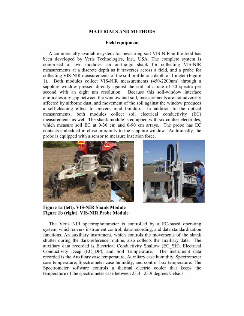
A commercially available system for measuring soil VIS-NIR in the field has been developed by Veris Technologies, Inc., USA. The complete system is comprised of two modules: an on-the-go shank for collecting VIS-NIR measurements at a discrete depth as it traverses across a field, and a probe for collecting VIS-NIR measurements of the soil profile to a depth of 1 meter (Figure 1). Both modules collect VIS-NIR measurements (450-2200nm) through a sapphire window pressed directly against the soil, at a rate of 20 spectra per second with an eight nm resolution. Because this soil-window interface eliminates any gap between the window and soil, measurements are not adversely affected by airborne dust, and movement of the soil against the window produces a self-cleaning effect to prevent mud buildup. In addition to the optical measurements, both modules collect soil electrical conductivity (EC) measurements as well. The shank module is equipped with six coulter electrodes, which measure soil EC at 0-30 cm and 0-90 cm arrays. The probe has EC contacts embedded in close proximity to the sapphire window. Additionally, the probe is equipped with a sensor to measure insertion force.

Figure 1a (left). VIS-NIR Shank Module

Figure 1b (right). VIS-NIR Probe Module The Veris NIR spectrophotometer is controlled by a PC-based operating system, which covers instrument control, data-recording, and data standardization functions. An auxiliary instrument, which controls the movements of the shank shutter during the dark-reference routine, also collects the auxiliary data. The auxiliary data recorded is Electrical Conductivity Shallow (EC_SH), Electrical Conductivity Deep (EC_DP), and Soil Temperature. The instrument data recorded is the Auxiliary case temperature, Auxiliary case humidity, Spectrometer case temperature, Spectrometer case humidity, and control box temperature. The Spectrometer software controls a thermal electric cooler that keeps the temperature of the spectrometer case between 23.4– 23.9 degrees Celsius.

Mapping and Sampling

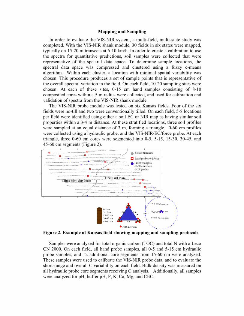
In order to evaluate the VIS-NIR system, a multi-field, multi-state study was completed. With the VIS-NIR shank module, 30 fields in six states were mapped, typically on 15-20 m transects at 6-10 km/h. In order to create a calibration to use the spectra for quantitative predictions, soil samples were collected that were representative of the spectral data space. To determine sample locations, the spectral data space was compressed and clustered using a fuzzy c-means algorithm. Within each cluster, a location with minimal spatial variability was chosen. This procedure produces a set of sample points that is representative of the overall spectral variation in the field. On each field, 10-20 sampling sites were chosen. At each of these sites, 0-15 cm hand samples consisting of 8-10 composited cores within a 5 m radius were collected, and used for calibration and validation of spectra from the VIS-NIR shank module. The VIS-NIR probe module was tested on six Kansas fields. Four of the six fields were no-till and two were conventionally tilled. On each field, 5-8 locations per field were identified using either a soil EC or NIR map as having similar soil properties within a 3-4 m distance. At these stratified locations, three soil profiles were sampled at an equal distance of 3 m, forming a triangle. 0-60 cm profiles were collected using a hydraulic probe, and the VIS-NIR/EC/force probe. At each triangle, three 0-60 cm cores were segmented into 0-5, 5-15, 15-30, 30-45, and 45-60 cm segments (Figure 2).

Figure 2. Example of Kansas field showing mapping and sampling protocols Samples were analyzed for total organic carbon (TOC) and total N with a Leco CN 2000. On each field, all hand probe samples, all 0-5 and 5-15 cm hydraulic probe samples, and 12 additional core segments from 15-60 cm were analyzed. These samples were used to calibrate the VIS-NIR probe data, and to evaluate the short-range and overall C variability on each field. Bulk density was measured on all hydraulic probe core segments receiving C analysis. Additionally, all samples were analyzed for pH, buffer pH, P, K, Ca, Mg, and CEC.

Calibration and Validation

The spectra were pretreated using the following pretreatments: spectra only, and spectra with SNV, 1st Derivative, 1st Derivative SNV, 2nd Derivative, and 2nd Derivative SNV. As the pretreatments were being completed, outliers were calculated using a Mahalanobis Distance algorithm. The outliers were removed and not used for the calibration. Each target (soil property of interest) was analyzed to remove outliers that were not within three times the standard deviation from the mean. In addition, each target was transformed using a Box-Cox transform and outliers were calculated the same way. Whichever method provided the least number of outliers was used for the calibration. All data were mean centered before the PLS regression was used to predict each sampled target value. For every calibration dataset, each pretreatment was applied and a target estimate was calculated, then for each target and pretreatment combination all auxiliary data was individually applied to calculate a target estimate. If any of the auxiliary data improved the calibration, multiple auxiliaries were added to see if there was continued improvement by including more information. All these possible calibrations were done automatically, and the best calibrations were selected at the end of the program. Once the calibration step decided the optimal calibrations for every target, those criteria were applied to the field data to make estimates. Field spectra was averaged and filtered as follows: 25 spectra were averaged to create a single set of spectra for each second, and field spectra were filtered with a Mahalanobis Distance algorithm. In this study, three validation methods were used: leave one out cross-validation, leave ½ of the data out, and leave one field out. Error and correlation statistics are based upon each set of predicted values.

Carbon measurement standards

In order to establish protocols for the measurement, monitoring, and verification of soil C change, a set of protocols was developed by the Nicholas Institute at Duke University (Willey and Chameides, 2007). The measurement standard calls for a sampling strategy that would achieve an error in the mean of 10% or less at the 90% confidence level. Based on anticipated rates of C change of 10% or less over a 10 year period (Willey and Chameides, 2007), there may not be a verifiable change in C, unless the confidence interval is kept small. Confidence intervals are based on the variability within a sampled area, and the number of samples. The costs required to significantly reduce confidence intervals may be cost-prohibitive, using conventional soil sampling and laboratory analysis. Proper use of on-the-go sensors may be able to affordably reduce confidence intervals, and two methods were tested on the six Kansas fields. First, using soil sensors maps to stratify fields into regions of similar values. This is a method of reducing variability within strata, although the Duke standard stipulates that strata boundaries must be based on biological reasoning (Willey and Chameides, 2007). Sampling triangles described above were selected from sensor maps in an attempt

to place these in areas of homogeneous soils, and to represent a full range of soil variability. This approach allowed standard deviations and confidence intervals to be compared by stratification method—none, field, soil type, and soil sensor. The second method tested involved using the sensor data points as soil ‘samples’. This method would release the power of intense measurements and, if effective, would have a significant effect on the confidence interval statistic. One of the key metrics in the second approach is measurement bias, and this was measured on the study fields. In order to evaluate the financial implications of various approaches, hypothetical carbon revenues were calculated and compared.

RESULTS

Overall results

Multiple fields in six states were mapped with the VIS-NIR shank module and sampled according the methods described above. Results show that VIS-NIR correlated well with C in four of the six states, with Ratio of Prediction to Deviation (RPD) scores of 2 or better (Table 1).

Table 1. Results of VIS-NIR C calibrations from 30 fields in 6 states.

When maps are generated from the calibration estimations and lab samples overlaid, the spatial structure of the field C levels and the correlation between the VIS-NIR system and lab-analyzed samples are evident (Figure 3).

Figure 3. C estimation from VIS-NIR shank module with lab values overlaid.

C Results--shank N RPD R² RMSE %C Std Dev. %C

6 Maryland fields 63 1.26 0.43 0.19 0.24

6 Illinois fields 64 3.26 0.9 0.23 0.75

6 Iowa fields 56 2.06 0.74 0.52 1.07

6 Kansas fields 64 2.00 0.76 0.14 0.27

5 Oklahoma fields 31 1.50 0.54 0.11 0.16

1 Nebraska field 10 2.79 0.86 0.15 0.41

Relationships to other properties were also evaluated (Figure 4). Interestingly, the VIS-NIR measurements on the Maryland fields were more highly correlated with P and K than with C. Two of the six Maryland fields had been treated with applications of municipal sludge and/or dairy manure, which may have contributed to these results.

Figure 4. Results for all measured soil properties in all four states.

In addition to the leave one sample out methodology, a leave one field out validation was also attempted on six fields from Illinois. This approach is a more rigorous test, as soil conditions, tillage, and other factors may vary between fields. A calibration that predicts well across this plurality of factors is especially robust. This more rigorous method showed that VIS-NIR can be a good predictor of soil properties, even without any calibration samples from the field (Figure 5).

Figure 5. Comparison of leave one out and leave one field out cross

validations.

Carbon measurements and confidence intervals

Results from the six fields in Kansas that were mapped with the VIS-NIR shank and probe modules and sampled using the methods described above, show that the probe sensors correlated well with C, with RPD scores of 1.8 or better. On four fields, the VIS-NIR shank achieved similar results (Table 2).

Table 2. Correlation and error statistics for Veris sensor measurements of carbon from six Kansas fields compared to laboratory measurements.

The array of sensors used in the probe—VIS-NIR, EC, and force, are frequently correlated to soil moisture, texture, and soil strength. As a result, this combination of measurements may be able to estimate bulk density, an important factor in measuring carbon change. While results were mixed, estimations of bulk density on three of the six fields were satisfactory (Table 3).

Table 3. Correlation and error statistics for Veris probe measurements of

bulk density compared to laboratory measurements.

N RPD R² RMSE SD

Drummond 27 1.11 0.21 0.12 0.14

Kejr 36 1.28 0.40 0.13 0.17

Lund_CT 23 2.09 0.76 0.07 0.14

Lund_NT 25 2.16 0.78 0.08 0.18

Markley 23 2.05 0.76 0.10 0.21

Tarn 12 1.59 0.61 0.11 0.17

Reducing confidence intervals: using sensor maps to stratify carbon zones

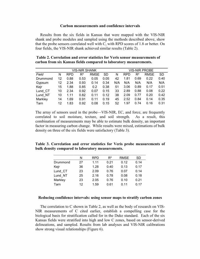
The correlation to C shown in Table 2, as well as the body of research on VIS-NIR measurements of C cited earlier, establish a compelling case for the biological basis for stratification called for in the Duke standard. Each of the six Kansas fields were stratified into high and low C zones, based on sensor-derived delineations, and sampled. Results from lab analyses and VIS-NIR calibrations show strong visual relationships (Figure 6).

VIS-NIR SHANK VIS-NIR PROBE

Field N RPD R² RMSE SD N RPD R² RMSE SD

Drummond 12 0.88 0.53 0.05 0.05 42 1.81 0.69 0.22 0.40

Gypsum 12 2.34 0.93 0.14 0.34 N/A N/A N/A N/A N/A

Kejr 15 1.88 0.85 0.2 0.38 51 3.06 0.89 0.17 0.51

Lund_CT 10 2.34 0.92 0.07 0.15 33 2.89 0.88 0.08 0.22

Lund_NT 10 1.11 0.82 0.11 0.12 38 2.09 0.77 0.20 0.42

Markley 14 1.69 0.91 0.11 0.19 45 2.52 0.84 0.14 0.35

Tarn 12 1.83 0.92 0.08 0.15 52 1.97 0.74 0.16 0.31

Figure 6. Kansas field example with all sample locations, and sensor data

calibrated to lab-analyzed % C. The confidence intervals obtained from sensor-based stratified sampling were compared with those from whole field sampling and NRCS soil survey-based stratification. The cores used in this analysis were collected with the hydraulic probe, with bulk density measured. This allows the carbon percentage to be expressed in Mg C per hectare. Results show a 25% reduction in confidence interval over whole field sampling and 13% reduction versus stratifying by soil survey soil units.

Table 4. Confidence interval comparison from various sampling

methodologies.

Reducing confidence intervals: using sensor data to increase sample number The on-the-go NIRS system delivers 200 to 400 readings per hectare depending upon speed and swath width. This high sample intensity greatly enhances the ability to estimate the mean carbon in the field with a minimum of variance. Specifically, if it is assumed that the carbon measurements are normally distributed and that the spatial coverage is uniform, the variance of the mean is:

2 2 /m s Nσ σ=

Confidence Intervals

whole field

soil type sensor strata

Drummond 1.59 1.59 1.30

Gypsum 2.76 2.77 2.34

Kejr 2.74 1.74 2.38

Lund CT 0.85 0.90 0.63

Lund NT 1.07 1.06 0.85

Markley 2.28 1.83 1.18

Tarn 1.65 1.68 0.93

All fields 0.68 0.60 0.51

where m designates the variance of the mean estimate, s designates the variance of the samples, and N is the number of samples in the average [Peebles, 2001]. Consequently, as N is increased the estimate improves. In the case of the carbon estimated by the VIS-NIR shank on the Kansas fields, the confidence interval is lowered to a miniscule amount (Table 5). This effect of averaging will apply to any type of carbon measurement. The actual confidence interval on the mean will be altered somewhat depending upon the accuracy of the instrument.

Table 5. Confidence intervals in % C from VIS-NIR shank data.

Measurement error can be broken down into two primary components: precision and accuracy. Precision describes how widely scattered replicate measurements would be while accuracy describes the position of these measurements relative to the true value. Any bias in the measurement would cause the estimates to be consistently high or low and thereby reduce accuracy. Such bias would not be reduced by averaging and would affect any estimate of the mean or total field carbon. Consequently, bias is an important measurement metric. For the six study fields in each of the four states, ½ of the samples were used for calibration and ½ for validation. Results show that VIS-NIR calibrations can be made with low bias (Table 6).

Table 6. Predicted % C and bias from multi-field multi-state studies.

Predicted

% C Actual % C Difference

Maryland 6 flds 1.2415 1.2187 0.0228

Iowa 6 flds 3.1757 3.2069 -0.0312

Illinois 6 flds 2.2650 2.2445 0.0205

Kansas 6 flds 1.1510 1.1649 -0.0138

Total 24 fields 1.9276 1.9279 -0.0003

Confidence Intervals % C

N Ave. % C Std dev Conf. Interval

Drummond 5875 1.164 0.05 0.001

Gypsum 3165 1.139 0.34 0.010

Kejr 4364 0.985 0.38 0.009

Lund CT 3291 1.188 0.15 0.004

Lund NT 860 1.303 0.12 0.007

Markley 2667 1.125 0.19 0.006

Tarn 4486 1.168 0.15 0.004

All fields 24708 1.153 0.20 0.002

Using sensor maps to vary nitrogen inputs

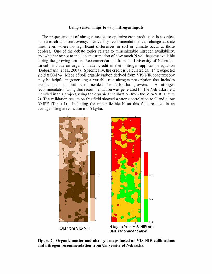
The proper amount of nitrogen needed to optimize crop production is a subject of research and controversy. University recommendations can change at state lines, even where no significant differences in soil or climate occur at those borders. One of the debate topics relates to mineralizable nitrogen availability, and whether or not to include an estimation of how much N will become available during the growing season. Recommendations from the University of Nebraska-Lincoln include an organic matter credit in their nitrogen application equation (Dobermann, et al., 2007). Specifically, the credit is calculated as: .14 x expected yield x OM %. Maps of soil organic carbon derived from VIS-NIR spectroscopy may be helpful in generating a variable rate nitrogen prescription that includes credits such as that recommended for Nebraska growers. A nitrogen recommendation using this recommendation was generated for the Nebraska field included in this project, using the organic C calibration from the VIS-NIR (Figure 7). The validation results on this field showed a strong correlation to C and a low RMSE (Table 1). Including the mineralizable N on this field resulted in an average nitrogen reduction of 56 kg/ha.

Figure 7. Organic matter and nitrogen maps based on VIS-NIR calibrations

and nitrogen recommendation from University of Nebraska.

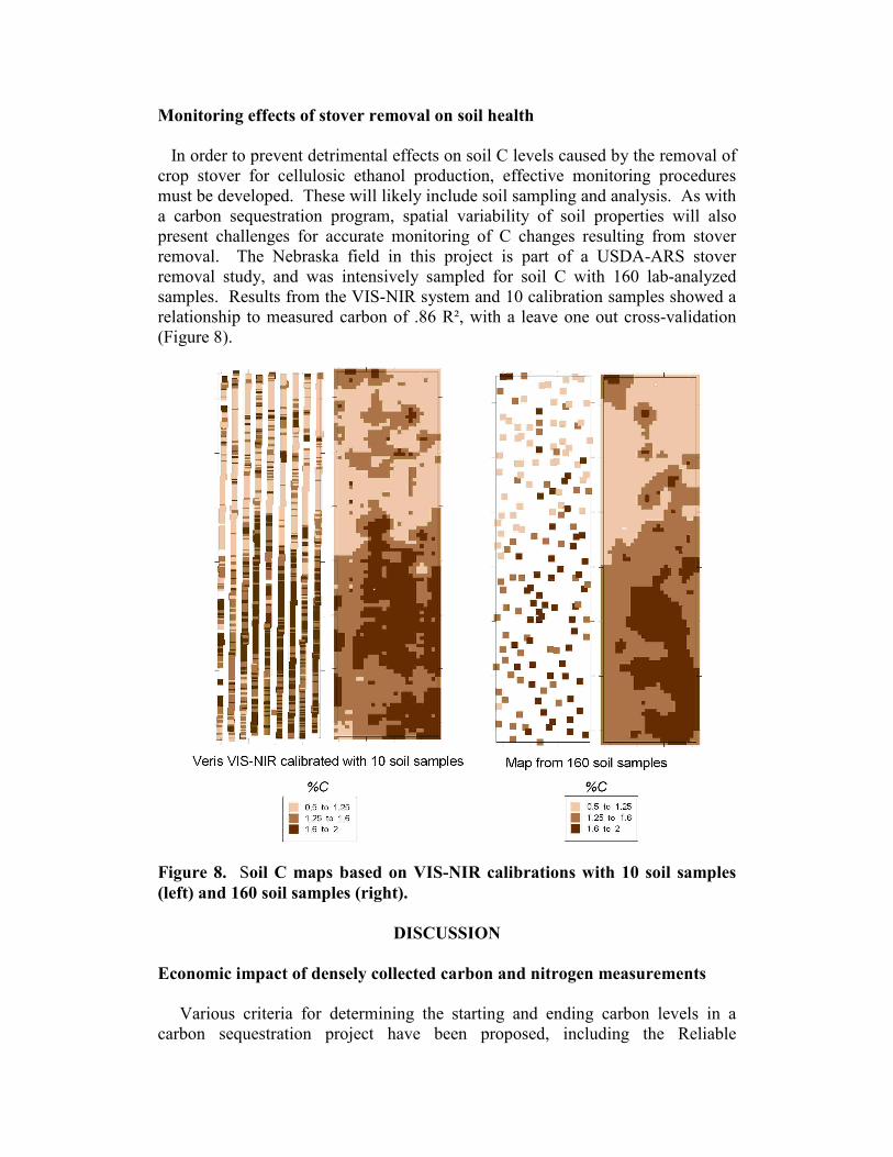
Monitoring effects of stover removal on soil health

In order to prevent detrimental effects on soil C levels caused by the removal of crop stover for cellulosic ethanol production, effective monitoring procedures must be developed. These will likely include soil sampling and analysis. As with a carbon sequestration program, spatial variability of soil properties will also present challenges for accurate monitoring of C changes resulting from stover removal. The Nebraska field in this project is part of a USDA-ARS stover removal study, and was intensively sampled for soil C with 160 lab-analyzed samples. Results from the VIS-NIR system and 10 calibration samples showed a relationship to measured carbon of .86 R², with a leave one out cross-validation (Figure 8).

Figure 8. Soil C maps based on VIS-NIR calibrations with 10 soil samples

(left) and 160 soil samples (right).

DISCUSSION

Economic impact of densely collected carbon and nitrogen measurements

Various criteria for determining the starting and ending carbon levels in a carbon sequestration project have been proposed, including the Reliable

Minimum Estimate (RME). This conservative method calculates the difference between the mean C plus confidence interval at the beginning, from the mean C minus confidence interval at the end (Brown et al., 2004). The result of using this approach on the amount of carbon measurable is shown on one of the Kansas fields (Table 7). On this 16 ha field, 18 samples would not be enough to discern any measurable carbon change, assuming an actual mean C change of 10% had actually occurred. Using sensors to stratify the field reduces the confidence interval and allows a C change of slightly less than one Mg/ha to be verified. If densely collected sensor data can be used to increase sample size, the effect on confidence intervals would be dramatic, with 92% of the mean C change able to be verified.

Table 7. Measurable RME of sequestered Mg C ha from various sampling

methodologies.

Method

90% C.I. N

Mean starting C

Mean starting C plus C.I.

Mean ending C (10% increase)

Mean ending C minus C.I.

Mg C ha measurable

Whole Field 1.65 18 27.3 28.95 30.03 28.38 -0.569

Sensor Strata 0.93 18 27.3 28.23 30.03 29.10 0.870

Sensors as samples 0.10 4486 27.3 27.40 30.03 29.93 2.521

Payment amounts for carbon offsets under a regulated carbon economy are unknown, however prices of $10-20/Mg have been suggested (Dole and Daschle, 2007). At those prices, each increase in measurable C of 0.1 Mg C ha would generate an additional $10-20/ha over a ten-year contract. The 25% lower confidence interval using the sensor stratification approach would generate $17-34/ha in additional revenue. Even more significant increases in measurable carbon could be achieved by using sensor measurements as samples, as shown in Table 7. The reduction in nitrogen rates made possible through detailed maps of soil organic carbon, can produce an economic return in two ways: One, the savings in nitrogen is immediate. At current fertilizer prices, the 56 kg/ha of N not needed on the field shown in Figure 7, represents a savings of over $50/ha. Second, reductions of applied nitrogen may also qualify for a greenhouse gas reduction payment in the future. The global warming potential of nitrous oxide gases is nearly 300 times that of CO2 on a per unit basis (Dalal et al., 2003). If growers are compensated for reductions in nitrous oxide emissions on a CO2 equivalent basis, the payments for a 56 kg/ha reduction could be more than $10/ha.

Improvements in measurements and interpretation

While the results from the six Kansas fields showed an advantage for stratification of carbon zones using sensors, future measurements should benefit from lessons learned in this initial attempt. These fields were stratified with out-of-state calibrations and with soil EC maps, as they were the first Kansas fields

mapped with the 450-2200 nm wavelength spectrometers. Using calibrations from local fields should help improve strata delineations. Only two strata, high and low C, were used. Expanding this to 3-5 strata could reduce variability within each stratum. Improvements in soil bulk density estimation may be achievable as well, by using larger diameter cores, and by improving probe VIS-NIR data quality in top few centimeters. Using sensor data to increase sample size is a crucial step in unleashing the power of intense measurements to reduce confidence intervals. An improved understanding of the bias and accuracy issues surrounding that strategy is needed. Highly detailed maps of soil C and soil N should be able to improve N efficiency. Some questions that arise are: can C:N ratios from VIS-NIR calibrations be used to better determine nitrogen mineralization potential? With VIS-NIR measurements achieving statistically significant correlations to other soil properties such as pH, calcium, and magnesium, and with EC sensors that relate to soil texture, can these datasets be mined to improve yield goals and estimates of nitrogen need? Could an initiative developed for carbon offset verification also generate map layers that empower a wider range of precision practices?

CONCLUSIONS

While exact criteria for measurements of soil C have not yet been established, VIS-NIR spectroscopy has shown an ability to reduce measurement confidence intervals. A reasonable improvement was found by delineating strata of similar carbon values. By using VIS-NIR to directly measure of soil C, the improvement in measurable carbon was rather significant. Both of these approaches require additional field research in a wider geographical range. The maps developed for soil carbon inventories can be used as a basis for variable rate nitrogen applications, provided N mineralization rates for organic carbon levels have been established.

REFERENCES

Adamchuk, V.I., J.W. Hummel, M.T. Morgan, and S.K. Upadhyaya. 2004. On- the-go soil sensors for precision agriculture. Computers and Electronics in Agriculture 44(1): 71 91. Adamchuk, V.I., E. Lund, T.M. Reed, R.B. Ferguson. 2007. Evaluation of an on- the-go technology for soil pH mapping. Precision Agric. 8:139-149 Brown, S, D. Shoch, T. Pearson, M. Delaney. 2004. Methods for Measuring and Monitoring Forestry Carbon Projects in California. Available on-line at: www.energy.ca.gov/reports/2004-10-29_500-04-072.PDF

Christy, C.D., P. Drummond, and D.A. Laird. 2003. An on-the-go Spectral Reflectance Sensor for Soil. ASAE Paper 031044. Presented at the 2003 ASAE annual meeting July 27-30, 2003. Las Vegas, NV. Dalal, R.C., W. Wang, G. P Robertson, and W.J. Parton. 2003. Nitrous Oxide Emission from Australian Agricultural Lands and Mitigation Options: a Review. Australian Journal of Soil Research 41 (2) 165-195 Dobermann, A., R. Ferguson, G. Hergert, C. Shapiro, D. Tarkalson, D.T. Walters, C. Wortmann. 2007. Nitrogen Response In High-Yielding Corn Systems Of Nebraska. Available on-line at: http://soilfertility.unl.edu Dole, R. and T. Daschle. 2007. Competing and Succeeding in the 21st Century.

21st Century Agriculture Policy Project. www.21stcenturyag.org Environmental Protection Agency. 2006. Nitrous Oxide Sources and Emissions. Available at: www.epa.gov.nitrousoxide/sources McBratney, A.B. and M.J. Pringle. 1997. Spatial variability in soil – implications for precision agriculture. In: Stafford, J. (Ed.), Precision Agriculture, 2. BIOS Scientific Publishing, Oxford, pp. 3-31. Peebles, Payton Z. Jr., 2001. Probability, Random Variables and Random Signal Principles. McGraw Hill. Reeves, J.B., G.W. McCarty, and J.J. Meisinger. 1999. Near infrared reflectance spectroscopy for the analysis of agricultural soils. Journal of Near Infrared Spectroscopy 9 (1), 25-34. Shibusawa, S., M.Z. Li, K Sakai, A. Sasao, and H. Sato, 1999. Spectrophotometer for real-time underground soil sensing. ASAE Paper No. 99-3030. St. Joseph, Mich.: ASAE. Sudduth, K.A. and J.W. Hummel. 1993. Portable, near-infrared spectrophotometer for rapid soil analysis. Transactions of the ASAE, vol. 36, pp. 185-193