Embed Size (px)
Citation preview

Theoretical Documentation
Version 2009
Soil & Water
Assessment Tool
TR-406

COLLEGE OF AGRICULTURE AND LIFE SCIENCES
TR-406
2011
Soil and Water Assessment Tool Theoretical Documentation
Version 2009
By S.L. Neitsch, J.G. Arnold, J.R. Kiniry, J.R. Williams
Grassland, Soil and Water Research Laboratory – Agricultural Research Service Blackland Research Center – Texas AgriLife Research
September 2011
Texas Water Resources Institute Technical Report No. 406 Texas A&M University System
College Station, Texas 77843-2118

SOIL AND WATER
ASSESSMENT TOOL THEORETICAL
DOCUMENTATION VERSION 2009
S.L. NEITSCH, J.G. ARNOLD, J.R. KINIRY, J.R. WILLIAMS
AUGUST, 2009
GRASSLAND, SOIL AND WATER RESEARCH LABORATORY ○ AGRICULTURAL RESEARCH SERVICE 808 EAST BLACKLAND ROAD ○ TEMPLE, TEXAS 76502
BLACKLAND RESEARCH CENTER ○ TEXAS AGRICULTURAL EXPERIMENT STATION
720 EAST BLACKLAND ROAD ○ TEMPLE, TEXAS 76502
TR-406


ACKNOWLEDGEMENTS The SWAT model is a continuation of thirty years of non-point source modeling. In addition to the Agricultural Research Service and Texas A&M University, several federal agencies including the US Environmental Protection Agency, Natural Resources Conservation Service, National Oceanic and Atmospheric Administration and Bureau of Indian Affairs have contributed to the model. We also want to thank all the state environmental agencies (with special thanks to Wisconsin Department of Natural Resources), state NRCS offices (with special thanks to the Texas State Office), numerous universities in the United States and abroad, and consultants who contributed to all aspects of the model. We appreciate your contributions and look forward to continued collaboration.


CONTENTS INTRODUCTION 1 0.1 DEVELOPMENT OF SWAT 3 0.2 OVERVIEW OF SWAT 6 LAND PHASE OF THE HYDROLOGIC CYCLE 9 ROUTING PHASE OF THE HYDROLOGIC CYCLE 21 0.3 REFERENCES 24
SECTION 1: CLIMATE
CHAPTER 1:1 EQUATIONS: ENERGY 29 1:1.1 SUN-EARTH RELATIONSHIPS 30 DISTANCE BETWEEN EARTH AND SUN 30 SOLAR DECLINATION 30 SOLAR NOON, SUNRISE, SUNSET, AND DAYLENGTH 31 1:1.2 SOLAR RADIATION 32 EXTRATERRESTRIAL RADIATION 32 SOLAR RADIATION UNDER CLOUDLESS SKIES 34 DAILY SOLAR RADIATION 34 HOURLY SOLAR RADIATION 35 DAILY NET RADIATION 36 1:1.3 TEMPERATURE 39 DAILY AIR TEMPERATURE 39

HOURLY AIR TEMPERATURE 40 SOIL TEMPERATURE 40 WATER TEMPERATURE 45 1:1.4 WIND SPEED 46 1:1.5 NOMENCLATURE 47 1:1.6 REFERENCES 49 CHAPTER 1:2 EQUATIONS: ATMOSPHERIC WATER 51 1:2.1 PRECIPITATION 52 1:2.2 MAXIMUM HALF-HOUR RAINFALL 53 1:2.3 WATER VAPOR 53 1:2.4 SNOW COVER 56 1:2.5 SNOW MELT 59 SNOW PACK TEMPERATURE 59 SNOW MELT EQUATION 60 1:2.6 NOMENCLATURE 61 1:2.7 REFERENCES 62 CHAPTER 1:3 EQUATIONS: WEATHER GENERATOR 65 1:3.1 PRECIPITATION 66 OCCURRENCE OF WET OR DRY DAY 66 AMOUNT OF PRECIPITATION 67 1:3.2 MAXIMUM HALF-HOUR RAINFALL 68 MONTHLY MAXIMUM HALF-HOUR RAIN 68 DAILY MAXIMUM HALF-HOUR RAIN VALUE 69 1:3.3 DISTRIBUTION OF RAINFALL WITHIN DAY 71 NORMALIZED INTENSITY DISTRIBUTION 71 GENERATED TIME TO PEAK INTENSITY 73 TOTAL RAINFALL AND DURATION 74 1:3.4 SOLAR RADIATION & TEMPERATURE 76 DAILY RESIDUALS 76 GENERATED VALUES 78 ADJUSTMENT FOR CLEAR/OVERCAST CONDITIONS 79 1:3.5 RELATIVE HUMIDITY 81 MEAN MONTHLY RELATIVE HUMIDITY 81 GENERATED DAILY VALUE 82

ADJUSTMENT FOR CLEAR/OVERCAST CONDITIONS 83 1:3.6 WIND SPEED 85 1:3.7 NOMENCLATURE 85 1:3.8 REFERENCES 87 CHAPTER 1:4 EQUATIONS: CLIMATE CUSTOMIZATION 90 1:4.1 ELEVATION BANDS 91 1:4.2 CLIMATE CHANGE 93 1:4.3 WEATHER FORECAST INCORPORATION 95 1:4.4 NOMENCLATURE 96
SECTION 2: HYDROLOGY
CHAPTER 2:1 EQUATIONS: SURFACE RUNOFF 98 2:1.1 RUNOFF VOLUME: SCS CURVE NUMBER PROCEDURE 99 SCS CURVE NUMBER 100 2:1.2 RUNOFF VOLUME: GREEN & AMPT INFILTRATION METHOD 107 2:1.3 PEAK RUNOFF RATE 110 TIME OF CONCENTRATION 110 RUNOFF COEFFICIENT 113 RAINFALL INTENSITY 114 MODIFIED RATIONAL FORMULA 115 2:1.4 SURFACE RUNOFF LAG 115 2:1.5 TRANSMISSION LOSSES 117 2:1.6 NOMENCLATURE 119 2:1.7 REFERENCES 120 CHAPTER 2:2 EQUATIONS: EVAPOTRANSPIRATION 123 2:2.1 CANOPY STORAGE 124 2:2.2 POTENTIAL EVAPOTRANSPIRATION 125 PENMAN-MONTEITH METHOD 126 PRIESTLEY-TAYLOR METHOD 132 HARGREAVES METHOD 132

2:2.3 ACTUAL EVAPOTRANSPIRATION 134 EVAPORATION OF INTERCEPTED RAINFALL 134 TRANSPIRATION 135 SUBLIMATION AND EVAPORATION FROM THE SOIL 135 2:2.4 NOMENCLATURE 140 2:2.5 REFERENCES 142 CHAPTER 2:3 EQUATIONS: SOIL WATER 146 2:3.1 SOIL STRUCTURE 147 2:3.2 PERCOLATION 151 2:3.3 BYPASS FLOW 152 2:3.4 PERCHED WATER TABLE 158 2:3.5 LATERAL FLOW 160 LATERAL FLOW LAG 162 2:3.6 NOMENCLATURE 164 2:3.7 REFERENCES 166
CHAPTER 2:4 EQUATIONS: GROUNDWATER 168 2:4.1 GROUNDWATER SYSTEMS 169 2:4.2 SHALLOW AQUIFER 171 RECHARGE 172 PARTITIONING OF RECHARGE BETWEEN SHALLOW AND DEEP AQUIFER 173
GROUNDWATER/BASE FLOW 173 REVAP 176 PUMPING 177 GROUNDWATER HEIGHT 177 2:4.3 DEEP AQUIFER 178 2:4.4 NOMENCLATURE 179 2:4.5 REFERENCES 180

SECTION 3: NUTRIENTS/PESTICIDES CHAPTER 3:1 EQUATIONS: NITROGEN 182 3:1.1 NITROGEN CYCLE IN THE SOIL 183 INITIALIZATION OF SOIL NITROGEN LEVELS 185 3:1.2 MINERALIZATION & DECOMPOSITION/ IMMOBILIZATION 187 HUMUS MINERALIZATION 188 RESIDUE DECOMPOSITION & MINERALIZATION 189 3:1.3 NITRIFICATION & AMMONIA VOLATILIZATION 191 3:1.4 DENITRIFICATION 194 3:1.5 ATMOSPHERIC DEPOSITION 195 NITROGEN IN RAINFALL 196 NITROGEN DRY DEPOSITION 197 3:1.6 FIXATION 198 3:1.7 UPWARD MOVEMENT OF NITRATE IN WATER 198 3:1.8 LEACHING 198 3:1.9 NITRATE IN THE SHALLOW AQUIFER 199 3:1.10 NOMENCLATURE 201 3:1.11 REFERENCES 203 CHAPTER 3:2 EQUATIONS: PHOSPHORUS 206 3:2.1 PHOSPHORUS CYCLE 207 INITIALIZATION OF SOIL PHOSPHORUS LEVELS 208 3:2.2 MINERALIZATION & DECOMPOSITION/ IMMOBILIZATION 210 HUMUS MINERALIZATION 211 RESIDUE DECOMPOSITION & MINERALIZATION 212 3:2.3 SORPTION OF INORGANIC P 214 3:2.4 LEACHING 216 3:2.5 PHOSPHORUS IN THE SHALLOW AQUIFER 217 3:2.6 NOMENCLATURE 217 3:2.7 REFERENCES 218

CHAPTER 3:3 EQUATIONS: PESTICIDES 221 3:3.1 WASH-OFF 222 3:3.2 DEGRADATION 223 3:3.3 LEACHING 225 3:3.4 NOMENCLATURE 225 3:3.5 REFERENCES 225
CHAPTER 3:4 EQUATIONS: BACTERIA 227 3:4.1 WASH-OFF 229 3:4.2 BACTERIA DIE-OFF/RE-GROWTH 229 3:4.3 LEACHING 233 3:4.4 NOMENCLATURE 234 3:4.5 REFERENCES 236
CHAPTER 3:5 EQUATIONS: CARBON 238 3:5.1 SUB-MODEL DESCRIPTION 239 3:5.2 CHANGES FROM PREVIOUS VERSION 243 3:5.3 ANALYTICAL SOLUTIONS 244 3:5.4 NOMENCLATURE 247 3:5.5 REFERENCES 248
SECTION 4: EROSION
CHAPTER 4:1 EQUATIONS: SEDIMENT 251 4:1.1 MUSLE 252 SOIL ERODIBILITY FACTOR 253 COVER AND MANAGEMENT FACTOR 256 SUPPORT PRACTICE FACTOR 257 TOPOGRAPHIC FACTOR 259 COARSE FRAGMENT FACTOR 259 4:1.2 USLE 260

RAINFALL ERODIBILITY INDEX 260 4:1.3 SNOW COVER EFFECTS 263 4:1.4 SEDIMENT LAG IN SURFACE RUNOFF 263 4:1.5 SEDIMENT IN LATERAL & GROUNDWATER FLOW 264 4:1.6 NOMENCLATURE 265 4:1.7 REFERENCES 266 CHAPTER 4:2 EQUATIONS: NUTRIENT TRANSPORT 268 4:2.1 NITRATE MOVEMENT 269 4:2.2 ORGANIC N IN SURFACE RUNOFF 271 ENRICHMENT RATIO 271 4:2.3 SOLUBLE PHOSPHORUS MOVEMENT 272 4:2.4 ORGANIC & MINERAL P ATTACHED TO SEDIMENT
IN SURFACE RUNOFF 273 ENRICHMENT RATIO 274 4:2.5 NUTRIENT LAG IN SURFACE RUNOFF AND LATERAL FLOW 275 4:2.6 NOMENCLATURE 276 4:2.7 REFERENCES 278 CHAPTER 4:3 EQUATIONS: PESTICIDE TRANSPORT 280 4:3.1 PHASE DISTRIBUTION OF PESTICIDE 281 4:3.2 MOVEMENT OF SOLUBLE PESTICIDE 282 4:3.3 TRANSPORT OF SORBED PESTICIDE 285 ENRICHMENT RATIO 286 4:3.4 PESTICIDE LAG IN SURFACE RUNOFF AND LATERAL FLOW 287 4:3.5 NOMENCLATURE 288 4:3.6 REFERENCES 289 CHAPTER 4:4 EQUATIONS: BACTERIA TRANSPORT 291 4:4.1 BACTERIA IN SURFACE RUNOFF 292 4:4.2 BACTERIA ATTACHED TO SEDIMENT IN SURFACE RUNOFF 292 ENRICHMENT RATIO 293 4:4.3 BACTERIA LAG IN SURFACE RUNOFF 294

4:4.4 NOMENCLATURE 296 CHAPTER 4:5 EQUATIONS: WATER QUALITY PARAMETERS 298 4:5.1 ALGAE 299 4:5.2 CARBONACEOUS BIOLOGICAL OXYGEN DEMAND 299 ENRICHMENT RATIO 300 4:5.3 DISSOLVED OXYGEN 301 OXYGEN SATURATION CONCENTRATION 301 4:5.4 NOMENCLATURE 302 4:5.5 REFERENCES 302
SECTION 5: LAND COVER/PLANT
CHAPTER 5:1 EQUATIONS: GROWTH CYCLE 304 5:1.1 HEAT UNITS 305 HEAT UNIT SCHEDULING 307 5:1.2 DORMANCY 310 5:1.3 PLANT TYPES 312 5:1.4 NOMENCLATURE 313 5:1.5 REFERENCES 314 CHAPTER 5:2 EQUATIONS: OPTIMAL GROWTH 316 5:2.1 POTENTIAL GROWTH 317
BIOMASS PRODUCTION 317 CANOPY COVER AND HEIGHT 321 ROOT DEVELOPMENT 324 MATURITY 325 5:2.2 WATER UPTAKE BY PLANTS 326 IMPACT OF LOW SOIL WATER CONTENT 328 ACTUAL WATER UPTAKE 329 5:2.3 NUTRIENT UPTAKE BY PLANTS 330 NITROGEN UPTAKE 330 PHOSPHORUS UPTAKE 335

5:2.4 CROP YIELD 338 5:2.5 NOMENCLATURE 340 5:2.6 REFERENCES 344 CHAPTER 5:3 EQUATIONS: ACTUAL GROWTH 346 19.1 GROWTH CONSTRAINTS 347 WATER STRESS 347 TEMPERATURE STRESS 347 NITROGEN STRESS 348 PHOSPHORUS STRESS 349 19.2 ACTUAL GROWTH 350 BIOMASS OVERRIDE 350 19.3 ACTUAL YIELD 351 HARVEST INDEX OVERRIDE 351 HARVEST EFFICIENCY 352 19.4 NOMENCLATURE 353
SECTION 6: MANAGEMENT PRACTICES
CHAPTER 6:1 EQUATIONS: GENERAL MANAGEMENT 355 6:1.1 PLANTING/BEGINNING OF GROWING SEASON 356 6:1.2 HARVEST OPERATION 357 6:1.3 GRAZING OPERATION 358 6:1.4 HARVEST & KILL OPERATION 359 6:1.5 KILL/END OF GROWING SEASON 360 6:1.6 TILLAGE 360 BIOLOGICAL MIXING 361 6:1.7 FERTILIZER APPLICATION 362 6:1.8 AUTO-APPLICATION OF FERTILIZER 365 6:1.9 CONTINUOUS APPLICATION OF FERTILIZER 368 6:1.10 PESTICIDE APPLICATION 369 6:1.11 NOMENCLATURE 371 6:1.12 REFERENCES 372

CHAPTER 6:2 EQUATIONS: WATER MANAGEMENT 374 6:2.1 IRRIGATION 375 MANUAL APPLICATION OF IRRIGATION 375 AUTO APPLICATION OF IRRIGATION 376 6:2.2 TILE DRAINAGE 377 6:2.3 IMPOUNDED/DEPRESSIONAL AREAS 377 6:2.4 WATER TRANSFER 378 6:2.5 CONSUMPTIVE WATER USE 378 6:2.6 POINT SOURCE LOADINGS 379 6:2.7 NOMENCLATURE 380
CHAPTER 6:3 EQUATIONS: URBAN AREAS 382 6:3.1 CHARACTERISTICS OF URBAN AREAS 383 6:3.2 SURFACE RUNOFF FROM URBAN AREAS 384 6:3.3 USGS REGRESSION EQUATIONS 385 6:3.4 BUILD UP/WASH OFF 386 STREET CLEANING 389 6:3.5 NOMENCLATURE 391 6:3.3 REFERENCES 392
CHAPTER 6:4 EQUATIONS: SEPTIC SYSTEMS 394 6:4.1 BIOZONE ALGORITHM 395 BUILDUP OF LIVE BACTERIAL BIOMASS 395 FATE AND TRANSPORT OF BACTERIA BIOMASS 396 FIELD CAPACITY 397 CLOGGING EFFECT ON HYDRAULIC CONDUCTIVITY 398 SOIL MOISTURE AND PERCOLATION 398 NITROGEN, BOD, FECAL COLIFORM 399 PHOSPHORUS REMOVAL 400 MODEL ASSUMPTIONS 401 6:4.2 INTEGRATION OF BIOZONE ALGORITHM 402 SIMULATING ACTIVE AND FAILING SYSTEMS 403 6:4.3 NOMENCLATURE 406

6:4.4 REFERENCES 407
CHAPTER 6:5 EQUATIONS: FILTER STRIPS AND GRASSED WATERWAYS 409 6:5.1 FILTER STRIPS 411 EMPERICAL MODEL DEVELOPMENT 411 SEDIMENT REDUCTION MODEL 414 NUTRIENT REDUCTION MODELS 416 VFS SWAT MODEL STRUCTURE 419 6:5.2 GRASSED WATERWAYS 421 6:5.3 NOMENCLATURE 423 6:5.4 REFERENCES 423
SECTION 7: MAIN CHANNEL PROCESSES
CHAPTER 7:1 EQUATIONS: WATER ROUTING 428 7:1.1 CHANNEL CHARACTERISTICS 429 7:1.2 FLOW RATE AND VELOCITY 431 7:1.3 VARIABLE STORAGE ROUTING METHOD 433 7:1.4 MUSKINGUM ROUTING METHOD 435 7:1.5 TRANSMISSION LOSSES 438 7:1.6 EVAPORATION LOSSES 439 7:1.7 BANK STORAGE 439 7:1.8 CHANNEL WATER BALANCE 441 7:1.9 NOMENCLATURE 442 7:1.10 REFERENCES 443 CHAPTER 7:2 EQUATIONS: SEDIMENT ROUTING 445 7:2.1 LANDSCAPE CONTRIBUTION TO SUBBASIN ROUTING 446 7:2.2 SEDIMENT ROUTING IN STREAM CHANNELS 447 SIMPLIFIED BANGOLD EQUATION 447 PHYSICS BASED APPROACH FOR CHANNEL EROSION 450

7:2.3 CHANNEL ERODIBILITY FACTOR 459 7:2.4 CHANNEL COVER FACTOR 460 7:2:5 CHANNEL DOWNCUTTING AND WIDENING 461 7:2.5 NOMENCLATURE 463 7:2.6 REFERENCES 464 CHAPTER 7:3 EQUATIONS: IN-STREAM NUTRIENT PROCESSES 467 7:3.1 ALGAE 468 CHLOROPHYLL A 468 ALGAL GROWTH 468 7:3.2 NITROGEN CYCLE 475 ORGANIC NITROGEN 475 AMMONIUM 476 NITRITE 477 NITRATE 478 7:3.3 PHOSPHORUS CYCLE 479 ORGANIC PHOSPHORUS 479 INORGANIC/SOLUBLE PHOSPHORUS 480 7:3.4 CARBONACEOUS BIOLOGICAL OXYGEN DEMAND 482 7:3.5 OXYGEN 483 OXYGEN SATURATION CONCENTRATION 484 REAERATION 485 7:3.6 NOMENCLATURE 488 7:3.7 REFERENCES 490 CHAPTER 7:4 EQUATIONS: IN-STREAM PESTICIDE TRANSFORMATIONS 493 7:4.1 PESTICIDE IN THE WATER 494 SOLID-LIQUID PARTITIONING 494 DEGREDATION 495 VOLATILIZATION 495 SETTLING 497 OUTFLOW 497 7:4.2 PESTICIDE IN THE SEDIMENT 498 SOLID-LIQUID PARTITIONING 498 DEGRADATION 499

RESUSPENSION 500 DIFFUSION 500 BURIAL 501 7:4.3 MASS BALANCE 501 7:4.4 NOMENCLATURE 502 7:4.5 REFERENCES 503
CHAPTER 7:5 EQUATIONS: BACTERIA ROUTING 505 7:5.1 BACTERIA DECAY 506 7:5.1 BACTERIA SEDIMENT 507 7:5.1 NOMENCLATURE 509 7:5.1 REFERENCES 509
CHAPTER 7:6 EQUATIONS: HEAVY METAL ROUTING 512
SECTION 8: WATER BODIES
CHAPTER 8:1 EQUATIONS: IMPOUNDMENT WATER ROUTING 514 8:1.1 RESERVOIRS 515 SURFACE AREA 516 PRECIPITATION 516 EVAPORATION 517 SEEPAGE 517 OUTFLOW 517 8:1.2 PONDS/WETLANDS 521 SURFACE AREA 522 PRECIPITATION 523 INFLOW 523
EVAPORATION 523 SEEPAGE 524 OUTFLOW 524 8:1.3 DEPRESSIONS/POTHOLES 526 SURFACE AREA 526

PRECIPITATION 527 INFLOW 527
EVAPORATION 528 SEEPAGE 528 OUTFLOW 529 8:1.4 NOMENCLATURE 530 8:1.5 REFERENCES 531 CHAPTER 8:2 EQUATIONS: SEDIMENT IN WATER BODIES 533 8:2.1 MASS BALANCE 534 8:2.2 SETTLING 534 8:2.3 SEDIMENT OUTFLOW 537 8:2.4 NOMENCLATURE 537 8:2.5 REFERENCES 537 CHAPTER 8:3 EQUATIONS: NUTRIENTS IN WATER BODIES 539 8:3.1 NUTRIENT TRANSFORMATIONS 540 8:3.2 TOTAL BALANCE 544 8:3.3 EUTROPHICATION 544 PHOSPHORUS/CHLOROPHYLL a CONCENTRATIONS 545 CHLOROPHYLL a/SECCHI DEPTH CORRELATIONS 546 8:3.4 NOMENCLATURE 547 8:3.5 REFERENCES 547
CHAPTER 8:4 EQUATIONS: PESTICIDES IN WATER BODIES 550 8:4.1 PESTICIDE IN THE WATER 551 SOLID-LIQUID PARTITIONING 551 DEGRADATION 552 VOLATILIZATION 553 SETTLING 554 OUTFLOW 555 8:4.2 PESTICIDE IN THE SEDIMENT 555

SOLID-LIQUID PARTITIONING 555 DEGRADATION 557 RESUSPENSION 557 DIFFUSION 558 BURIAL 559 8:4.3 MASS BALANCE 559 8:4.4 NOMENCLATURE 560 8:4.5 REFERENCES 561 CHAPTER 8:5 EQUATIONS: BACTERIA IN WATER BODIES 563 8:5.1 BACTERIA DECAY 564 8:5.2 NOMENCLATURE 565 8:5.3 REFERENCES 565 APPENDIX A LIST OF VARIABLES 567
APPENDIX B REFERENCES 597

SOIL AND WATER ASSESSMENT TOOL

1
INTRODUCTION
SWAT is the acronym for Soil and Water Assessment Tool, a river
basin, or watershed, scale model developed by Dr. Jeff Arnold for the USDA
Agricultural Research Service (ARS). SWAT was developed to predict the impact
of land management practices on water, sediment and agricultural chemical yields
in large complex watersheds with varying soils, land use and management
conditions over long periods of time. To satisfy this objective, the model
is physically based. Rather than incorporating regression equations to
describe the relationship between input and output variables, SWAT
requires specific information about weather, soil properties,
topography, vegetation, and land management practices occurring in
the watershed. The physical processes associated with water

2 SWAT THEORETICAL DOCUMENTATION, VERSION 2009
movement, sediment movement, crop growth, nutrient cycling, etc. are
directly modeled by SWAT using this input data.
Benefits of this approach are
watersheds with no monitoring data (e.g. stream gage data) can be modeled
the relative impact of alternative input data (e.g. changes in management practices, climate, vegetation, etc.) on water quality or other variables of interest can be quantified
uses readily available inputs. While SWAT can be used to study more
specialized processes such as bacteria transport, the minimum data
required to make a run are commonly available from government
agencies.
is computationally efficient. Simulation of very large basins or a
variety of management strategies can be performed without excessive
investment of time or money.
enables users to study long-term impacts. Many of the problems
currently addressed by users involve the gradual buildup of pollutants
and the impact on downstream water bodies. To study these types of
problems, results are needed from runs with output spanning several
decades.
SWAT is a continuous time model, i.e. a long-term yield model. The
model is not designed to simulate detailed, single-event flood routing.

INTRODUCTION 3
0.1 DEVELOPMENT OF SWAT
SWAT incorporates features of several ARS models and is a direct
outgrowth of the SWRRB1 model (Simulator for Water Resources in Rural
Basins) (Williams et al., 1985; Arnold et al., 1990). Specific models that
contributed significantly to the development of SWAT were CREAMS2
(Chemicals, Runoff, and Erosion from Agricultural Management Systems)
(Knisel, 1980), GLEAMS3 (Groundwater Loading Effects on Agricultural
Management Systems) (Leonard et al., 1987), and EPIC4 (Erosion-Productivity
Impact Calculator) (Williams et al., 1984).
Development of SWRRB began with modification of the daily rainfall
hydrology model from CREAMS. The major changes made to the CREAMS
hydrology model were: a) the model was expanded to allow simultaneous
computations on several subbasins to predict basin water yield; b) a groundwater
or return flow component was added; c) a reservoir storage component was added
to calculate the effect of farm ponds and reservoirs on water and sediment yield;
d) a weather simulation model incorporating data for rainfall, solar radiation, and
temperature was added to facilitate long-term simulations and provide temporally
and spatially representative weather; e) the method for predicting the peak runoff
rates was improved; f) the EPIC crop growth model was added to account for
annual variation in growth; g) a simple flood routing component was added; h)
sediment transport components were added to simulate sediment movement
1 SWRRB is a continuous time step model that was developed to simulate nonpoint source loadings from watersheds. 2 In response to the Clean Water Act, ARS assembled a team of interdisciplinary scientists from across the U.S. to develop a process -based, nonpoint source simulation model in the early 1970s. From that effort CREAMS was developed. CREAMS is a field scale model designed to simulate the impact of land management on water, sediment, nutrients and pesticides leaving the edge of the field. A number of other ARS models such as GLEAMS, EPIC, SWRRB and AGNPS trace their origins to the CREAMS model. 3 GLEAMS is a nonpoint source model which focuses on pesticide and nutrient groundwater loadings. 4 EPIC was originally developed to simulate the impact of erosion on crop productivity and has now evolved into a comprehensive agricultural management, field scale, nonpoint source loading model.
4 SWAT THEORETICAL DOCUMENTATION, VERSION 2009
through ponds, reservoirs, streams and valleys; and i) calculation of transmission
losses was incorporated.
The primary focus of model use in the late 1980s was water quality
assessment and development of SWRRB reflected this emphasis. Notable
modifications of SWRRB at this time included incorporation of: a) the GLEAMS
pesticide fate component; b) optional SCS technology for estimating peak runoff
rates; and c) newly developed sediment yield equations. These modifications
extended the model’s capability to deal with a wide variety of watershed
management problems.
In the late 1980s, the Bureau of Indian Affairs needed a model to estimate
the downstream impact of water management within Indian reservation lands in
Arizona and New Mexico. While SWRRB was easily utilized for watersheds up
to a few hundred square kilometers in size, the Bureau also wanted to simulate
stream flow for basins extending over several thousand square kilometers. For an
area this extensive, the watershed under study needed to be divided into several
hundred subbasins. Watershed division in SWRRB was limited to ten subbasins
and the model routed water and sediment transported out of the subbasins directly
to the watershed outlet. These limitations led to the development of a model
called ROTO (Routing Outputs to Outlet) (Arnold et al., 1995), which took output
from multiple SWRRB runs and routed the flows through channels and reservoirs.
ROTO provided a reach routing approach and overcame the SWRRB subbasin
limitation by “linking” multiple SWRRB runs together. Although this approach
was effective, the input and output of multiple SWRRB files was cumbersome
and required considerable computer storage. In addition, all SWRRB runs had to
be made independently and then input to ROTO for the channel and reservoir
routing. To overcome the awkwardness of this arrangement, SWRRB and ROTO
were merged into a single model, SWAT. While allowing simulations of very
extensive areas, SWAT retained all the features which made SWRRB such a
valuable simulation model.

INTRODUCTION 5
Since SWAT was created in the early 1990s, it has undergone continued
review and expansion of capabilities. The most significant improvements of the
model between releases include:
SWAT94.2: Multiple hydrologic response units (HRUs) incorporated.
SWAT96.2: Auto-fertilization and auto-irrigation added as
management options; canopy storage of water incorporated; a CO2
component added to crop growth model for climatic change studies;
Penman-Monteith potential evapotranspiration equation added; lateral
flow of water in the soil based on kinematic storage model
incorporated; in-stream nutrient water quality equations from
QUAL2E added; in-stream pesticide routing.
SWAT98.1: Snow melt routines improved; in-stream water quality
improved; nutrient cycling routines expanded; grazing, manure
applications, and tile flow drainage added as management options;
model modified for use in Southern Hemisphere.
SWAT99.2: Nutrient cycling routines improved, rice/wetland routines
improved, reservoir/pond/wetland nutrient removal by settling added;
bank storage of water in reach added; routing of metals through reach
added; all year references in model changed from last 2 digits of year
to 4-digit year; urban build up/wash off equations from SWMM added
along with regression equations from USGS.
SWAT2000: Bacteria transport routines added; Green & Ampt
infiltration added; weather generator improved; allow daily solar
radiation, relative humidity, and wind speed to be read in or generated;
allow potential ET values for watershed to be read in or calculated; all
potential ET methods reviewed; elevation band processes improved;
enabled simulation of unlimited number of reservoirs; Muskingum
routing method added; modified dormancy calculations for proper
simulation in tropical areas.
6 SWAT THEORETICAL DOCUMENTATION, VERSION 2009
SWAT2009: Bacteria transport routines improved; weather forecast
scenarios added; subdaily precipitation generator added; the retention
parameter used in the daily CN calculation may be a function of soil
water content or plant evapotranspiration; update to vegetative filter
strip model; wet and dry deposition of nitrate and ammonium
improved; modeling of on-site wastewater systems.
In addition to the changes listed above, interfaces for the model have been
developed in Windows (Visual Basic), GRASS, and ArcView. SWAT has also
undergone extensive validation.
0.2 OVERVIEW OF SWAT
SWAT allows a number of different physical processes to be simulated in
a watershed. These processes will be briefly summarized in this section. For more
detailed discussions of the various procedures, please consult the chapter devoted
to the topic of interest.
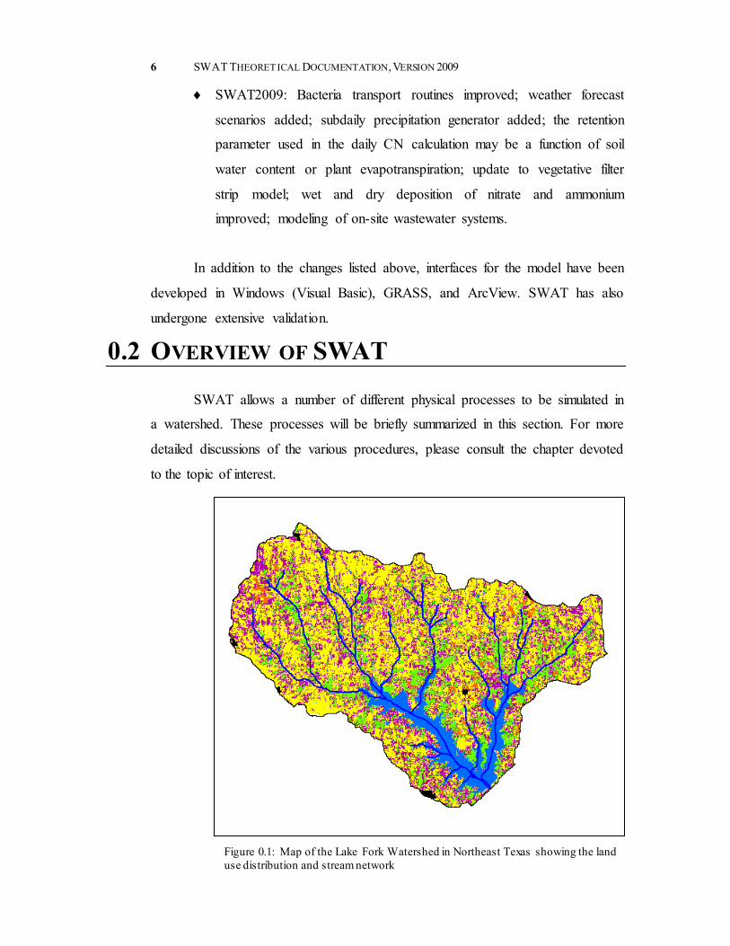
Figure 0.1: Map of the Lake Fork Watershed in Northeast Texas showing the land use distribution and stream network
INTRODUCTION 7
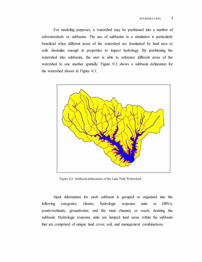
For modeling purposes, a watershed may be partitioned into a number of
subwatersheds or subbasins. The use of subbasins in a simulation is particularly
beneficial when different areas of the watershed are dominated by land uses or
soils dissimilar enough in properties to impact hydrology. By partitioning the
watershed into subbasins, the user is able to reference different areas of the
watershed to one another spatially. Figure 0.2 shows a subbasin delineation for
the watershed shown in Figure 0.1.
Input information for each subbasin is grouped or organized into the
following categories: climate; hydrologic response units or HRUs;
ponds/wetlands; groundwater; and the main channel, or reach, draining the
subbasin. Hydrologic response units are lumped land areas within the subbasin
that are comprised of unique land cover, soil, and management combinations.
Figure 0.2: Subbasin delineation of the Lake Fork Watershed.

8 SWAT THEORETICAL DOCUMENTATION, VERSION 2009
No matter what type of problem studied with SWAT, water balance is the
driving force behind everything that happens in the watershed. To accurately
predict the movement of pesticides, sediments or nutrients, the hydrologic cycle
as simulated by the model must conform to what is happening in the watershed.
Simulation of the hydrology of a watershed can be separated into two major
divisions. The first division is the land phase of the hydrologic cycle, depicted in
Figure 0.3. The land phase of the hydrologic cycle controls the amount of water,
sediment, nutrient and pesticide loadings to the main channel in each subbasin.
The second division is the water or routing phase of the hydrologic cycle which
can be defined as the movement of water, sediments, etc. through the channel
network of the watershed to the outlet.
Figure 0.3: Schematic representation of the hydrologic cycle.
INTRODUCTION 9
0.2.1 LAND PHASE OF THE HYDROLOGIC CYCLE The hydrologic cycle as simulated by SWAT is based on the water balance
equation:
)(1
0 gwseepasurfday
t
i
t QwEQRSWSW
where SWt is the final soil water content (mm H2O), SW0 is the initial soil water
content on day i (mm H2O), t is the time (days), Rday is the amount of precipitation
on day i (mm H2O), Qsurf is the amount of surface runoff on day i (mm H2O), Ea is
the amount of evapotranspiration on day i (mm H2O), wseep is the amount of water
entering the vadose zone from the soil profile on day i (mm H2O), and Qgw is the
amount of return flow on day i (mm H2O).
The subdivision of the watershed enables the model to reflect differences
in evapotranspiration for various crops and soils. Runoff is predicted separately
for each HRU and routed to obtain the total runoff for the watershed. This
increases accuracy and gives a much better physical description of the water
balance.
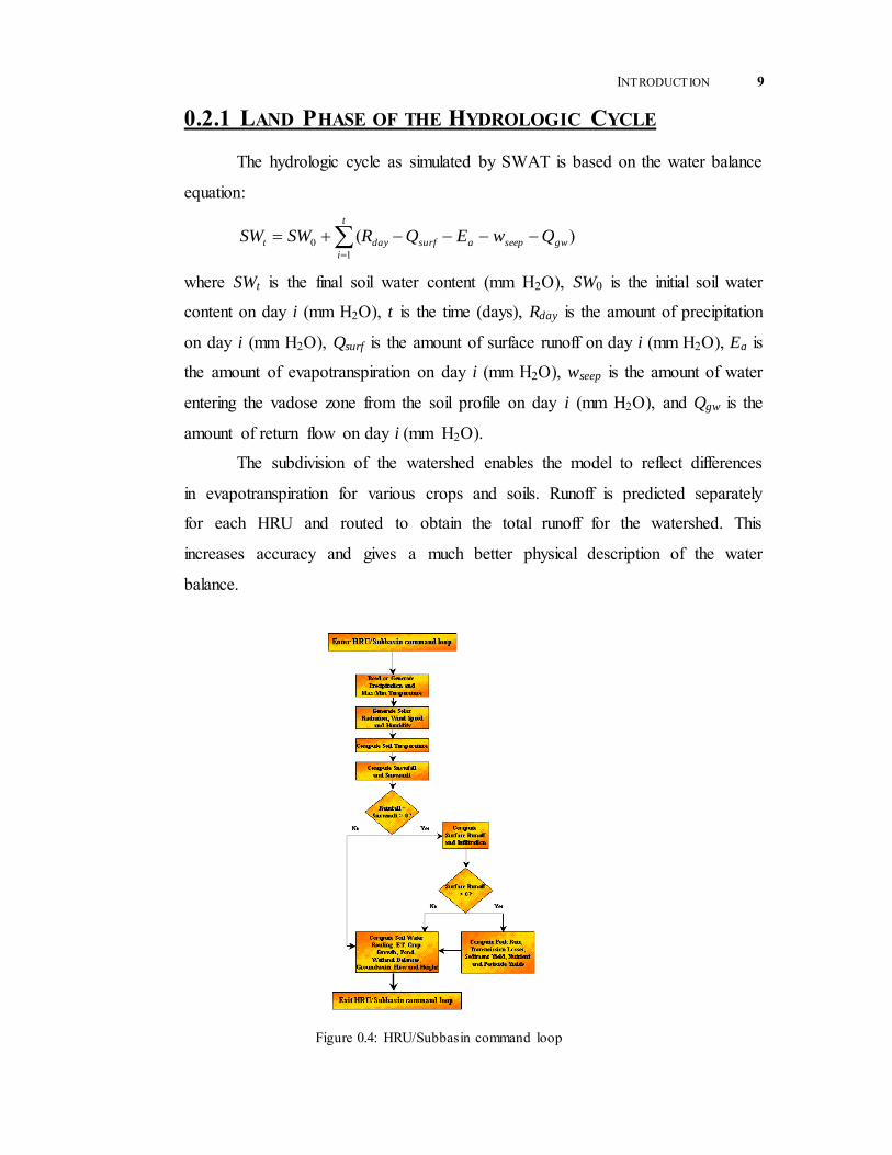
Figure 0.4: HRU/Subbasin command loop

10 SWAT THEORETICAL DOCUMENTATION, VERSION 2009
Figure 0.4 shows the general sequence of processes used by SWAT to
model the land phase of the hydrologic cycle. The different inputs and processes
involved in this phase of the hydrologic cycle are summarized in the following
sections.
0.2.1.1 CLIMATE
The climate of a watershed provides the moisture and energy inputs that
control the water balance and determine the relative importance of the different
components of the hydrologic cycle.
The climatic variables required by SWAT consist of daily precipitation,
maximum/minimum air temperature, solar radiation, wind speed and relative
humidity. The model allows values for daily precipitation, maximum/minimum
air temperatures, solar radiation, wind speed and relative humidity to be input
from records of observed data or generated during the simulation.
WEATHER GENERATOR. Daily values for weather are generated from average monthly values. The model generates a set of weather data for each subbasin. The values for any one subbasin will be generated independently and there will be no spatial correlation of generated values between the different subbasins.
GENERATED PRECIPITATION. SWAT uses a model developed by Nicks (1974) to generate daily precipitation for simulations which do not read in measured data. This precipitation model is also used to fill in missing data in the measured records. The precipitation generator uses a first-order Markov chain model to define a day as wet or dry by comparing a random number (0.0-1.0) generated by the model to monthly wet-dry probabilities input by the user. If the day is classified as wet, the amount of precipitation is generated from a skewed distribution or a modified exponential distribution.
SUB-DAILY RAINFALL PATTERNS. If sub-daily precipitation values are needed, a double exponential function is used to represent the intensity patterns within a storm. With the double exponential distribution, rainfall intensity exponentially increases with time to a maximum, or peak, intensity. Once the peak intensity is reached, the rainfall intensity exponentially decreases with time until the end of the storm GENERATED AIR TEMPERATURE AND SOLAR RADIATION. Maximum and minimum air temperatures and solar radiation are generated from a normal distribution. A continuity equation is incorporated into the generator to

INTRODUCTION 11
account for temperature and radiation variations caused by dry vs. rainy conditions. Maximum air temperature and solar radiation are adjusted downward when simulating rainy conditions and upwards when simulating dry conditions. The adjustments are made so that the long-term generated values for the average monthly maximum temperature and monthly solar radiation agree with the input averages. GENERATED WIND SPEED. A modified exponential equation is used to generate daily mean wind speed given the mean monthly wind speed. GENERATED RELATIVE HUMIDITY. The relative humidity model uses a triangular distribution to simulate the daily average relative humidity from the monthly average. As with temperature and radiation, the mean daily relative humidity is adjusted to account for wet- and dry-day effects.
SNOW. SWAT classifies precipitation as rain or freezing rain/snow using the average daily temperature.
SNOW COVER. The snow cover component of SWAT has been updated from a simple, uniform snow cover model to a more complex model which allows non-uniform cover due to shading, drifting, topography and land cover. The user defines a threshold snow depth above which snow coverage will always extend over 100% of the area. As the snow depth in a subbasin decreases below this value, the snow coverage is allowed to decline non-linearly based on an areal depletion curve. SNOW MELT. Snow melt is controlled by the air and snow pack temperature, the melting rate, and the areal coverage of snow. If snow is present, it is melted on days when the maximum temperature exceeds 0C using a linear function of the difference between the average snow pack-maximum air temperature and the base or threshold temperature for snow melt. Melted snow is treated the same as rainfall for estimating runoff and percolation. For snow melt, rainfall energy is set to zero and the peak runoff rate is estimated assuming uniformly melted snow for a 24 hour duration. ELEVATION BANDS. The model allows the subbasin to be split into a maximum of ten elevation bands. Snow cover and snow melt are simulated separately for each elevation band. By dividing the subbasin into elevation bands, the model is able to assess the differences in snow cover and snow melt caused by orographic variation in precipitation and temperature.
SOIL TEMPERATURE. Soil temperature impacts water movement and the decay rate of residue in the soil. Daily average soil temperature is calculated at the soil surface and the center of each soil layer. The temperature of the soil surface is a function of snow cover, plant cover and residue cover, the bare soil surface temperature, and the previous day’s soil surface temperature. The temperature of a soil layer is a function of the surface temperature, mean annual air temperature and the depth in the soil at which variation in temperature due to changes in

12 SWAT THEORETICAL DOCUMENTATION, VERSION 2009
climatic conditions no longer occurs. This depth, referred to as the damping depth, is dependent upon the bulk density and the soil water content. 0.2.1.2 HYDROLOGY As precipitation descends, it may be intercepted and held in the vegetation
canopy or fall to the soil surface. Water on the soil surface will infiltrate into the
soil profile or flow overland as runoff. Runoff moves relatively quickly toward a
stream channel and contributes to short-term stream response. Infiltrated water
may be held in the soil and later evapotranspired or it may slowly make its way to
the surface-water system via underground paths. The potential pathways of water
movement simulated by SWAT in the HRU are illustrated in Figure 0.5.
CANOPY STORAGE. Canopy storage is the water intercepted by vegetative surfaces (the canopy) where it is held and made available for evaporation. When using the curve number method to compute surface runoff, canopy storage is taken into account in the surface runoff calculations. However, if methods such as Green & Ampt are used to model infiltration and runoff, canopy storage must be modeled separately. SWAT allows the user to input the maximum amount of water that can be stored in the canopy at the maximum leaf area index for the land cover. This value and the leaf area index are used by the model to compute the maximum storage at any time in the growth cycle of the land cover/crop. When evaporation is computed, water is first removed from canopy storage. INFILTRATION. Infiltration refers to the entry of water into a soil profile from the soil surface. As infiltration continues, the soil becomes increasingly wet, causing the rate of infiltration to decrease with time until it reaches a steady value. The initial rate of infiltration depends on the moisture content of the soil prior to the introduction of water at the soil surface. The final rate of infiltration is equivalent to the saturated hydraulic conductivity of the soil. Because the curve number method used to calculate surface runoff operates on a daily time-step, it is unable to directly model infiltration. The amount of water entering the soil profile is calculated as the difference between the amount of rainfall and the amount of surface runoff. The Green & Ampt infiltration method does directly model infiltration, but it requires precipitation data in smaller time increments. REDISTRIBUTION. Redistribution refers to the continued movement of water through a soil profile after input of water (via precipitation or irrigation) has ceased at the soil surface. Redistribution is caused by differences in water content in the profile. Once the water content throughout the entire profile is uniform, g

INTRODUCTION 13

14 SWAT THEORETICAL DOCUMENTATION, VERSION 2009
redistribution will cease. The redistribution component of SWAT uses a storage routing technique to predict flow through each soil layer in the root zone. Downward flow, or percolation, occurs when field capacity of a soil layer is exceeded and the layer below is not saturated. The flow rate is governed by the saturated conductivity of the soil layer. Redistribution is affected by soil temperature. If the temperature in a particular layer is 0C or below, no redistribution is allowed from that layer. EVAPOTRANSPIRATION. Evapotranspiration is a collective term for all processes by which water in the liquid or solid phase at or near the earth's surface becomes atmospheric water vapor. Evapotranspiration includes evaporation from rivers and lakes, bare soil, and vegetative surfaces; evaporation from within the leaves of plants (transpiration); and sublimation from ice and snow surfaces. The model computes evaporation from soils and plants separately as described by Ritchie (1972). Potential soil water evaporation is estimated as a function of potential evapotranspiration and leaf area index (area of plant leaves relative to the area of the HRU). Actual soil water evaporation is estimated by using exponential functions of soil depth and water content. Plant transpiration is simulated as a linear function of potential evapotranspiration and leaf area index.
POTENTIAL EVAPOTRANSPIRATION. Potential evapotranspiration is the rate at which evapotranspiration would occur from a large area completely and uniformly covered with growing vegetation which has access to an unlimited supply of soil water. This rate is assumed to be unaffected by micro-climatic processes such as advection or heat-storage effects. The model offers three options for estimating potential evapotranspiration: Hargreaves (Hargreaves et al., 1985), Priestley-Taylor (Priestley and Taylor, 1972), and Penman-Monteith (Monteith, 1965).
LATERAL SUBSURFACE FLOW. Lateral subsurface flow, or interflow, is streamflow contribution which originates below the surface but above the zone where rocks are saturated with water. Lateral subsurface flow in the soil profile (0-2m) is calculated simultaneously with redistribution. A kinematic storage model is used to predict lateral flow in each soil layer. The model accounts for variation in conductivity, slope and soil water content. SURFACE RUNOFF. Surface runoff, or overland flow, is flow that occurs along a sloping surface. Using daily or subdaily rainfall amounts, SWAT simulates surface runoff volumes and peak runoff rates for each HRU.
SURFACE RUNOFF VOLUME is computed using a modification of the SCS curve number method (USDA Soil Conservation Service, 1972) or the Green & Ampt infiltration method (Green and Ampt, 1911). In the curve number method, the curve number varies non-linearly with the moisture content of the soil. The curve number drops as the soil approaches the wilting point and increases to near 100 as the soil approaches saturation. The Green & Ampt method requires sub-daily precipitation data and calculates infiltration as a function of the wetting front matric potential and effective hydraulic conductivity. Water that does not infiltrate

INTRODUCTION 15
becomes surface runoff. SWAT includes a provision for estimating runoff from frozen soil where a soil is defined as frozen if the temperature in the first soil layer is less than 0°C. The model increases runoff for frozen soils but still allows significant infiltration when the frozen soils are dry.
PEAK RUNOFF RATE predictions are made with a modification of the rational method. In brief, the rational method is based on the idea that if a rainfall of intensity i begins instantaneously and continues indefinitely, the rate of runoff will increase until the time of concentration, tc, when all of the subbasin is contributing to flow at the outlet. In the modified Rational Formula, the peak runoff rate is a function of the proportion of daily precipitation that falls during the subbasin tc, the daily surface runoff volume, and the subbasin time of concentration. The proportion of rainfall occurring during the subbasin tc is estimated as a function of total daily rainfall using a stochastic technique. The subbasin time of concentration is estimated using Manning’s Formula considering both overland and channel flow.
PONDS. Ponds are water storage structures located within a subbasin which intercept surface runoff. The catchment area of a pond is defined as a fraction of the total area of the subbasin. Ponds are assumed to be located off the main channel in a subbasin and will never receive water from upstream subbasins. Pond water storage is a function of pond capacity, daily inflows and outflows, seepage and evaporation. Required inputs are the storage capacity and surface area of the pond when filled to capacity. Surface area below capacity is estimated as a non-linear function of storage.
TRIBUTARY CHANNELS. Two types of channels are defined within a subbasin: the main channel and tributary channels. Tributary channels are minor or lower order channels branching off the main channel within the subbasin. Each tributary channel within a subbasin drains only a portion of the subbasin and does not receive groundwater contribution to its flow. All flow in the tributary channels is released and routed through the main channel of the subbasin. SWAT uses the attributes of tributary channels to determine the time of concentration for the subbasin.
TRANSMISSION LOSSES. Transmission losses are losses of surface flow via leaching through the streambed. This type of loss occurs in ephemeral or intermittent streams where groundwater contribution occurs only at certain times of the year, or not at all. SWAT uses Lane’s method described in Chapter 19 of the SCS Hydrology Handbook (USDA Soil Conservation Service, 1983) to estimate transmission losses. Water losses from the channel are a function of channel width and length and flow duration. Both runoff volume and peak rate are adjusted when transmission losses occur in tributary channels.
RETURN FLOW. Return flow, or base flow, is the volume of streamflow originating from groundwater. SWAT partitions groundwater into two aquifer systems: a shallow, unconfined aquifer which contributes return flow to streams

16 SWAT THEORETICAL DOCUMENTATION, VERSION 2009
within the watershed and a deep, confined aquifer which contributes return flow to streams outside the watershed (Arnold et al., 1993). Water percolating past the bottom of the root zone is partitioned into two fractions—each fraction becomes recharge for one of the aquifers. In addition to return flow, water stored in the shallow aquifer may replenish moisture in the soil profile in very dry conditions or be directly removed by plant. Water in the shallow or deep aquifer may be removed by pumping.
0.2.1.3 LAND COVER/PLANT GROWTH SWAT utilizes a single plant growth model to simulate all types of land
covers. The model is able to differentiate between annual and perennial plants.
Annual plants grow from the planting date to the harvest date or until the
accumulated heat units equal the potential heat units for the plant. Perennial plants
maintain their root systems throughout the year, becoming dormant in the winter
months. They resume growth when the average daily air temperature exceeds the
minimum, or base, temperature required. The plant growth model is used to assess
removal of water and nutrients from the root zone, transpiration, and
biomass/yield production.
POTENTIAL GROWTH. The potential increase in plant biomass on a given day is defined as the increase in biomass under ideal growing conditions. The potential increase in biomass for a day is a function of intercepted energy and the plant's efficiency in converting energy to biomass. Energy interception is estimated as a function of solar radiation and the plant’s leaf area index. POTENTIAL AND ACTUAL TRANSPIRATION. The process used to calculate potential plant transpiration is described in the section on evapotranspiration. Actual transpiration is a function of potential transpiration and soil water availability.
NUTRIENT UPTAKE. Plant use of nitrogen and phosphorus are estimated with a supply and demand approach where the daily plant nitrogen and phosphorus demands are calculated as the difference between the actual concentration of the element in the plant and the optimal concentration. The optimal concentration of the elements varies with growth stage as described by Jones (1983). GROWTH CONTRAINTS. Potential plant growth and yield are usually not achieved due to constraints imposed by the environment. The model estimates stresses caused by water, nutrients and temperature.

INTRODUCTION 17
0.2.1.4 EROSION
Erosion and sediment yield are estimated for each HRU with the Modified
Universal Soil Loss Equation (MUSLE) (Williams, 1975). While the USLE uses
rainfall as an indicator of erosive energy, MUSLE uses the amount of runoff to
simulate erosion and sediment yield. The substitution results in a number of
benefits: the prediction accuracy of the model is increased, the need for a delivery
ratio is eliminated, and single storm estimates of sediment yields can be
calculated. The hydrology model supplies estimates of runoff volume and peak
runoff rate which, with the subbasin area, are used to calculate the runoff erosive
energy variable. The crop management factor is recalculated every day that runoff
occurs. It is a function of above-ground biomass, residue on the soil surface, and
the minimum C factor for the plant. Other factors of the erosion equation are
evaluated as described by Wischmeier and Smith (1978).
0.2.1.5 NUTRIENTS
SWAT tracks the movement and transformation of several forms of
nitrogen and phosphorus in the watershed. In the soil, transformation of nitrogen
from one form to another is governed by the nitrogen cycle as depicted in Figure
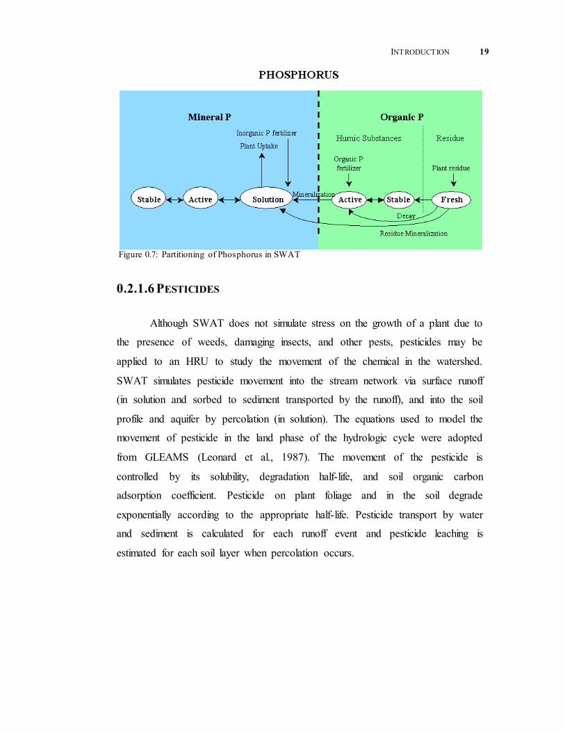
0.6. The transformation of phosphorus in the soil is controlled by the phosphorus
cycle shown in Figure 0.7. Nutrients may be introduced to the main channel and
transported downstream through surface runoff and lateral subsurface flow.
NITROGEN. The different processes modeled by SWAT in the HRUs and the various pools of nitrogen in the soil are depicted in Figure 1.6. Plant use of nitrogen is estimated using the supply and demand approach described in the section on plant growth. In addition to plant use, nitrate and organic N may be removed from the soil via mass flow of water. Amounts of NO3-N contained in runoff, lateral flow and percolation are estimated as products of the volume of water and the average concentration of nitrate in the layer. Organic N transport with sediment is calculated with a loading function developed by McElroy et al. (1976) and modified by Williams and Hann (1978) for application to individual runoff events. The loading function estimates the daily organic N runoff loss based on the concentration of organic N in the top soil layer, the sediment yield, and the enrichment ratio. The enrichment ratio is the concentration of organic N in the sediment divided by that in the soil.

18 SWAT THEORETICAL DOCUMENTATION, VERSION 2009
Figure 0.6: Partitioning of Nitrogen in SWAT
PHOSPHORUS. The different processes modeled by SWAT in the HRUs and the various pools of phosphorus in the soil are depicted in Figure 1.7. Plant use of phosphorus is estimated using the supply and demand approach described in the section on plant growth. In addition to plant use, soluble phosphorus and organic P may be removed from the soil via mass flow of water. Phosphorus is not a mobile nutrient and interaction between surface runoff with solution P in the top 10 mm of soil will not be complete. The amount of soluble P removed in runoff is predicted using solution P concentration in the top 10 mm of soil, the runoff volume and a partitioning factor. Sediment transport of P is simulated with a loading function as described in organic N transport.
INTRODUCTION 19
Figure 0.7: Partitioning of Phosphorus in SWAT
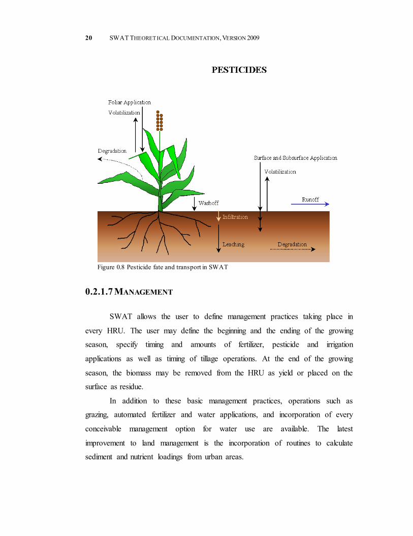
0.2.1.6 PESTICIDES Although SWAT does not simulate stress on the growth of a plant due to
the presence of weeds, damaging insects, and other pests, pesticides may be
applied to an HRU to study the movement of the chemical in the watershed.
SWAT simulates pesticide movement into the stream network via surface runoff
(in solution and sorbed to sediment transported by the runoff), and into the soil
profile and aquifer by percolation (in solution). The equations used to model the
movement of pesticide in the land phase of the hydrologic cycle were adopted
from GLEAMS (Leonard et al., 1987). The movement of the pesticide is
controlled by its solubility, degradation half-life, and soil organic carbon
adsorption coefficient. Pesticide on plant foliage and in the soil degrade
exponentially according to the appropriate half-life. Pesticide transport by water
and sediment is calculated for each runoff event and pesticide leaching is
estimated for each soil layer when percolation occurs.
20 SWAT THEORETICAL DOCUMENTATION, VERSION 2009
Figure 0.8 Pesticide fate and transport in SWAT
0.2.1.7 MANAGEMENT SWAT allows the user to define management practices taking place in
every HRU. The user may define the beginning and the ending of the growing
season, specify timing and amounts of fertilizer, pesticide and irrigation
applications as well as timing of tillage operations. At the end of the growing
season, the biomass may be removed from the HRU as yield or placed on the
surface as residue.
In addition to these basic management practices, operations such as
grazing, automated fertilizer and water applications, and incorporation of every
conceivable management option for water use are available. The latest
improvement to land management is the incorporation of routines to calculate
sediment and nutrient loadings from urban areas.

INTRODUCTION 21
ROTATIONS. The dictionary defines a rotation as the growing of different crops in succession in one field, usually in a regular sequence. A rotation in SWAT refers to a change in management practices from one year to the next. There is no limit to the number of years of different management operations specified in a rotation. SWAT also does not limit the number of land cover/crops grown within one year in the HRU. However, only one land cover can be growing at any one time.
WATER USE. The two most typical uses of water are for application to agricultural lands or use as a town's water supply. SWAT allows water to be applied on an HRU from any water source within or outside the watershed. Water may also be transferred between reservoirs, reaches and subbasins as well as exported from the watershed.
0.2.2 ROUTING PHASE OF THE HYDROLOGIC CYCLE
Once SWAT determines the loadings of water, sediment, nutrients and
pesticides to the main channel, the loadings are routed through the stream network
of the watershed using a command structure similar to that of HYMO (Williams
and Hann, 1972). In addition to keeping track of mass flow in the channel, SWAT
models the transformation of chemicals in the stream and streambed. Figure 0.9
illustrates the different in-stream processes modeled by SWAT.
Figure 0.9: In-stream processes modeled by SWAT

22 SWAT THEORETICAL DOCUMENTATION, VERSION 2009
0.2.2.1 ROUTING IN THE MAIN CHANNEL OR REACH Routing in the main channel can be divided into four components: water,
sediment, nutrients and organic chemicals.
FLOOD ROUTING. As water flows downstream, a portion may be lost due to evaporation and transmission through the bed of the channel. Another potential loss is removal of water from the channel for agricultural or human use. Flow may be supplemented by the fall of rain directly on the channel and/or addition of water from point source discharges. Flow is routed through the channel using a variable storage coefficient method developed by Williams (1969) or the Muskingum routing method. SEDIMENT ROUTING. The transport of sediment in the channel is controlled by the simultaneous operation of two processes, deposition and degradation. Previous versions of SWAT used stream power to estimate deposition/degradation in the channels (Arnold et al, 1995). Bagnold (1977) defined stream power as the product of water density, flow rate and water surface slope. Williams (1980) used Bagnold’s definition of stream power to develop a method for determining degradation as a function of channel slope and velocity. In this version of SWAT, the equations have been simplified and the maximum amount of sediment that can be transported from a reach segment is a function of the peak channel velocity. Available stream power is used to reentrain loose and deposited material until all of the material is removed. Excess stream power causes bed degradation. Bed degradation is adjusted for stream bed erodibility and cover. NUTRIENT ROUTING. Nutrient transformations in the stream are controlled by the in-stream water quality component of the model. The in-stream kinetics used in SWAT for nutrient routing are adapted from QUAL2E (Brown and Barnwell, 1987). The model tracks nutrients dissolved in the stream and nutrients adsorbed to the sediment. Dissolved nutrients are transported with the water while those sorbed to sediments are allowed to be deposited with the sediment on the bed of the channel. CHANNEL PESTICIDE ROUTING. While an unlimited number of pesticides may be applied to the HRUs, only one pesticide may be routed through the channel network of the watershed due to the complexity of the processes simulated. As with the nutrients, the total pesticide load in the channel is partitioned into dissolved and sediment-attached components. While the dissolved pesticide is transported with water, the pesticide attached to sediment is affected by sediment transport and deposition processes. Pesticide transformations in the dissolved and sorbed phases are governed by first-order decay relationships. The major in-stream processes simulated by the model are settling, burial, resuspension, volatilization, diffusion and transformation.

INTRODUCTION 23
0.2.2.2 ROUTING IN THE RESERVOIR The water balance for reservoirs includes inflow, outflow, rainfall on the
surface, evaporation, seepage from the reservoir bottom and diversions.
RESERVOIR OUTFLOW. The model offers three alternatives for estimating outflow from the reservoir. The first option allows the user to input measured outflow. The second option, designed for small, uncontrolled reservoirs, requires the users to specify a water release rate. When the reservoir volume exceeds the principle storage, the extra water is released at the specified rate. Volume exceeding the emergency spillway is released within one day. The third option, designed for larger, managed reservoirs, has the user specify monthly target volumes for the reservoir. SEDIMENT ROUTING. Sediment inflow may originate from transport through the upstream reaches or from surface runoff within the subbasin. The concentration of sediment in the reservoir is estimated using a simple continuity equation based on volume and concentration of inflow, outflow, and water retained in the reservoir. Settling of sediment in the reservoir is governed by an equilibrium sediment concentration and the median sediment particle size. The amount of sediment in the reservoir outflow is the product of the volume of water flowing out of the reservoir and the suspended sediment concentration in the reservoir at the time of release.
RESERVOIR NUTRIENTS. A simple model for nitrogen and phosphorus mass balance was taken from Chapra (1997). The model assumes: 1) the lake is completely mixed; 2) phosphorus is the limiting nutrient; and, 3) total phosphorus is a measure of the lake trophic status. The first assumption ignores lake stratification and intensification of phytoplankton in the epilimnon. The second assumption is generally valid when non-point sources dominate and the third assumption implies that a relationship exists between total phosphorus and biomass. The phosphorus mass balance equation includes the concentration in the lake, inflow, outflow and overall loss rate. RESERVOIR PESTICIDES. The lake pesticide balance model is taken from Chapra (1997) and assumes well mixed conditions. The system is partitioned into a well mixed surface water layer underlain by a well mixed sediment layer. The pesticide is partitioned into dissolved and particulate phases in both the water and sediment layers. The major processes simulated by the model are loading, outflow, transformation, volatilization, settling, diffusion, resuspension and burial.

24 SWAT THEORETICAL DOCUMENTATION, VERSION 2009
0.3 REFERENCES
Arnold, J.G., P.M. Allen, and G. Bernhardt. 1993. A comprehensive surface-
groundwater flow model. J. Hydrol. 142:47-69.
Arnold, J.G., J.R. Williams, A.D. Nicks, and N.B. Sammons. 1990. SWRRB: A
basin scale simulation model for soil and water resources management.
Texas A&M Univ. Press, College Station, TX.
Arnold, J.G., J.R. Williams and D.R. Maidment. 1995. Continuous-time water and
sediment-routing model for large basins. Journal of Hydraulic Engineering
121(2):171-183.
Bagnold, R.A. 1977. Bedload transport in natural rivers. Water Resources Res.
13(2):303-312.
Brown, L.C. and T.O. Barnwell, Jr. 1987. The enhanced water quality models
QUAL2E and QUAL2E-UNCAS documentation and user manual. EPA
document EPA/600/3-87/007. USEPA, Athens, GA.
Chapra, S.C. 1997. Surface water-quality modeling. McGraw-Hill, Boston.
Green, W.H. and G.A. Ampt. 1911. Studies on soil physics, 1. The flow of air and
water through soils. Journal of Agricultural Sciences 4:11-24.
Hargreaves, G.L., G.H. Hargreaves, and J.P. Riley. 1985. Agricultural benefits for
Senegal River Basin. J. Irrig. and Drain. Engr. 111(2):113-124.
Jones, C.A. 1983. A survey of the variability in tissue nitrogen and phosphorus
concentrations in maize and grain sorghum. Field Crops Res. 6:133-147.
Knisel, W.G. 1980. CREAMS, a field scale model for chemicals, runoff and
erosion from agricultural management systems. USDA Conservation
Research Rept. No. 26.
Leonard, R.A. and R.D. Wauchope. 1980. Chapter 5: The pesticide submodel. p.
88-112. In Knisel, W.G. (ed). CREAMS: A field-scale model for
chemicals, runoff, and erosion from agricultural management systems.
U.S. Department of Agriculture, Conservation research report no. 26.

INTRODUCTION 25
Leonard, R.A., W.G. Knisel, and D.A. Still. 1987. GLEAMS: Groundwater
loading effects on agricultural management systems. Trans. ASAE
30(5):1403-1428.
McElroy, A.D., S.Y. Chiu, J.W. Nebgen, A. Aleti, and F.W. Bennett. 1976.
Loading functions for assessment of water pollution from nonpoint
sources. EPA document EPA 600/2-76-151. USEPA, Athens, GA.
Monteith, J.L. 1965. Evaporation and the environment. p. 205-234. In The state
and movement of water in living organisms. 19th Symposia of the Society
for Experimental Biology. Cambridge Univ. Press, London, U.K.
Nicks, A.D. 1974. Stochastic generation of the occurrence, pattern and location of
maximum amount of daily rainfall. p. 154-171. In Proc. Symp. Statistical
Hydrology, Tucson, AZ. Aug.-Sept. 1971. USDA Misc. Publ. 1275. U.S.
Gov. Print. Office, Washington, DC.
Priestley, C.H.B. and R.J. Taylor. 1972. On the assessment of surface heat flux
and evaporation using large-scale parameters. Mon. Weather Rev. 100:81-
92.
Ritchie, J.T. 1972. A model for predicting evaporation from a row crop with
incomplete cover. Water Resour. Res. 8:1204-1213.
USDA Soil Conservation Service. 1983. National Engineering Handbook Section
4 Hydrology, Chapter 19.
USDA Soil Conservation Service. 1972. National Engineering Handbook Section
4 Hydrology, Chapters 4-10.
Williams, J.R. 1980. SPNM, a model for predicting sediment, phosphorus, and
nitrogen yields from agricultural basins. Water Resour. Bull. 16(5):843-
848.
Williams, J.R. 1975. Sediment routing for agricultural watersheds. Water Resour.
Bull. 11(5):965-974.
Williams, J.R. 1969. Flood routing with variable travel time or variable storage
coefficients. Trans. ASAE 12(1):100-103.
Williams, J.R., A.D. Nicks, and J.G. Arnold. 1985. Simulator for water resources
in rural basins. Journal of Hydraulic Engineering 111(6): 970-986.

26 SWAT THEORETICAL DOCUMENTATION, VERSION 2009
Williams, J.R. and R.W. Hann. 1978. Optimal operation of large agricultural
watersheds with water quality constraints. Texas Water Resources
Institute, Texas A&M Univ., Tech. Rept. No. 96.
Williams, J.R. and R.W. Hann. 1972. HYMO, a problem-oriented computer
language for building hydrologic models. Water Resour. Res. 8(1):79-85.
Williams, J.R., C.A. Jones and P.T. Dyke. 1984. A modeling approach to
determining the relationship between erosion and soil productivity. Trans.
ASAE 27(1):129-144.
Wischmeier, W.H., and D.D. Smith. 1978. Predicting rainfall losses: A guide to
conservation planning. USDA Agricultural Handbook No. 537. U.S. Gov.
Print. Office, Washington, D. C.

INTRODUCTION 27

CLIMATE
The climatic inputs to the model are
reviewed first because it is these inputs that
provide the moisture and energy that drive
all other processes simulated in the
watershed. The climatic processes modeled
in SWAT consist of precipitation, air
temperature, soil temperature and solar
radiation. Depending on the method used to
calculate potential evapotranspiration, wind
speed and relative humidity may also be
modeled.

29
SECTION 1 CHAPTER 1
EQUATIONS:
ENERGY
Once water is introduced to the system as precipitation, the available
energy, specifically solar radiation, exerts a major control on the movement of
water in the land phase of the hydrologic cycle. Processes that are greatly affected
by temperature and solar radiation include snow fall, snow melt and evaporation.
Since evaporation is the primary water removal mechanism in the watershed, the
energy inputs become very important in reproducing or simulating an accurate
water balance.

30 SWAT THEORETICAL DOCUMENTATION, VERSION 2009
1:1.1 SUN-EARTH RELATIONSHIPS
A number of basic concepts related to the earth's orbit around the sun are
required by the model to make solar radiation calculations. This section
summarizes these concepts. Iqbal (1983) provides a detailed discussion of these
and other topics related to solar radiation for users who require more information.
1:1.1.1 DISTANCE BETWEEN EARTH AND SUN The mean distance between the earth and the sun is 1.496 x 10⁸ km and is
called one astronomical unit (AU). The earth revolves around the sun in an
elliptical orbit and the distance from the earth to the sun on a given day will vary
from a maximum of 1.017 AU to a minimum of 0.983 AU.
An accurate value of the earth-sun distance is important because the solar
radiation reaching the earth is inversely proportional to the square of its distance
from the sun. The distance is traditionally expressed in mathematical form as a
Fourier series type of expansion with a number of coefficients. For most
engineering applications a simple expression used by Duffie and Beckman (1980)
is adequate for calculating the reciprocal of the square of the radius vector of the
earth, also called the eccentricity correction factor, E0, of the earth's orbit:
3652cos033.01200 ndrrE 1:1.1.1
where r0 is the mean earth-sun distance (1 AU), r is the earth-sun distance for any
given day of the year (AU), and dn is the day number of the year, ranging from 1
on January 1 to 365 on December 31. February is always assumed to have 28
days, making the accuracy of the equation vary due to the leap year cycle.
1:1.1.2 SOLAR DECLINATION The solar declination is the earth's latitude at which incoming solar rays
are normal to the earth's surface. The solar declination is zero at the spring and
fall equinoxes, approximately +23½° at the summer solstice and approximately
-23½° at the winter solstice.
A simple formula to calculate solar declination from Perrin de
Brichambaut (1975) is:

CHAPTER 1:1: EQUATIONS—ENERGY 31
82
3652sin4.0sin 1
nd
1:1.1.2
where δ is the solar declination reported in radians, and dn is the day number of
the year.
1:1.1.3 SOLAR NOON, SUNRISE, SUNSET AND DAYLENGTH The angle between the line from an observer on the earth to the sun
and a vertical line extending upward from the observer is called the zenith angle,
θz (Figure 1:1-1). Solar noon occurs when this angle is at its minimum value for
the day.
Figure 1:1-1: Diagram illustrating zenith angle
For a given geographical position, the relationship between the sun and a
horizontal surface on the earth's surface is:
tz coscoscossinsincos 1:1.1.3
where δ is the solar declination in radians, is the geographic latitude in radians,
is the angular velocity of the earth's rotation (0.2618 rad h-1 or 15˚ h-1), and t is
the solar hour. t equals zero at solar noon, is a positive value in the morning and is
a negative value in the evening. The combined term t is referred to as the hour
angle.
Sunrise, TSR, and sunset, TSS, occur at equal times before and after solar
noon. These times can be determined by rearranging the above equation as:

32 SWAT THEORETICAL DOCUMENTATION, VERSION 2009
tantancos 1
SRT 1:1.1.4
and
tantancos 1
SST 1:1.1.5
Total daylength, TDL, is calculated:
tantancos2 1
DLT 1:1.1.6
At latitudes above 66.5 or below -66.5, the absolute value of [-tan tan] can
exceed 1 and the above equation cannot be used. When this happens, there is
either no sunrise (winter) or no sunset (summer) and TDL must be assigned a value
of 0 or 24 hours, respectively.
To determine the minimum daylength that will occur during the year,
equation 1:1.1.6 is solved with the solar declination set to -23.5 (-0.4102 radians)
for the northern hemisphere or +23.5 (0.4102 radians) for the southern
hemisphere.
The only SWAT input variable used in the calculations reviewed in
Section 1:1.1 is given in Table 1:1-1.
Table 1:1-1: SWAT input variables that used in earth-sun relationship calculations.
Variable name
Definition
File Name
SUB_LAT Latitude of the subbasin (degrees). .sub
1:1.2 SOLAR RADIATION
1:1.2.1 EXTRATERRESTRIAL RADIATION The radiant energy from the sun is practically the only source of energy
that impacts climatic processes on earth. The solar constant, ISC, is the rate of total
solar energy at all wavelengths incident on a unit area exposed normally to rays of
the sun at a distance of 1 AU from the sun. Quantifying this value has been the

CHAPTER 1:1: EQUATIONS—ENERGY 33
object of numerous studies through the years. The value officially adopted by the
Commission for Instruments and Methods of Observation in October 1981 is
ISC = 1367 W m-2 = 4.921 MJ m-2 h-1
On any given day, the extraterrestrial irradiance (rate of energy) on a
surface normal to the rays of the sun, I0n, is:
00 EII SCn 1:1.2.1
where E0 is the eccentricity correction factor of the earth's orbit, and I0n has the
same units as the solar constant, ISC.
To calculate the irradiance on a horizontal surface, I0,
zSCzn EIII coscos 000 1:1.2.2
where cos θz is defined in equation 1:1.1.3.
The amount of energy falling on a horizontal surface during a day is given
by
ssss
srdtIdtIH
0 000 2 1:1.2.3
where H0 is the extraterrestrial daily irradiation (MJ m-2 d-1), sr is sunrise, and ss
is sunset. Assuming that E0 remains constant during the one day time step and
converting the time dt to the hour angle, the equation can be written
SRT
SC tdtEIH
000 coscoscossinsin24 1:1.2.4
or
SRSRSC TTEIH
sincoscossinsin2400 1:1.2.5
where ISC is the solar constant (4.921 MJ m-2 h-1), E0 is the eccentricity correction
factor of the earth's orbit, is the angular velocity of the earth's rotation (0.2618
rad h-1), the hour of sunrise, TSR, is defined by equation 1:1.1.4, δ is the solar
declination in radians, and is the geographic latitude in radians. Multiplying all
the constants together gives
SRSR TTEH sincoscossinsin59.37 00 1:1.2.6

34 SWAT THEORETICAL DOCUMENTATION, VERSION 2009
1:1.2.2 SOLAR RADIATION UNDER CLOUDLESS SKIES When solar radiation enters the earth's atmosphere, a portion of the energy
is removed by scattering and adsorption. The amount of energy lost is a function
of the transmittance of the atmosphere, the composition and concentration of the
constituents of air at the location, the path length the radiation travels through the
air column, and the radiation wavelength.
Due to the complexity of the process and the detail of the information
required to accurately predict the amount of radiant energy lost while passing
through the atmosphere, SWAT makes a broad assumption that roughly 20% of
the extraterrestrial radiation is lost while passing through the atmosphere under
cloudless skies. Using this assumption, the maximum possible solar radiation,
HMX, at a particular location on the earth's surface is calculated as:
SRSRMX TTEH sincoscossinsin0.30 0 1:1.2.7
where the maximum possible solar radiation, HMX, is the amount of radiation
reaching the earth's surface under a clear sky (MJ m-2 d-1).
1:1.2.3 DAILY SOLAR RADIATION The solar radiation reaching the earth's surface on a given day, Hday, may
be less than HMX due to the presence of cloud cover. The daily solar radiation data
required by SWAT may be read from an input file or generated by the model.
The variable SLRSIM in the master watershed (file.cio) file identifies the
method used to obtain solar radiation data. To read in daily solar radiation data, the
variable is set to 1 and the name of the solar radiation data file and the number of
solar radiation records stored in the file are set. To generate daily solar radiation
values, SLRSIM is set to 2. The equations used to generate solar radiation data in
SWAT are reviewed in Chapter 1:3. SWAT input variables that pertain to solar
radiation are summarized in Table 1:1-2.

CHAPTER 1:1: EQUATIONS—ENERGY 35
Table 1:1-2: SWAT input variables used in solar radiation calculations. Variable
name
Definition File
Name SUB_LAT Latitude of the subbasin (degrees). .sub SLRSIM Solar radiation input code: 1-measured, 2-generated file.cio NSTOT Number of solar radiation records within the .slr file (required if SLRSIM = 1) file.cio SLRFILE Name of measured solar radiation input file (.slr) (required if SLRSIM = 1) file.cio ISGAGE Number of solar radiation record used within the subbasin (required if
SLRSIM = 1) .sub
see description of .slr file in the User’s Manual for input and format requirements if measured
daily solar radiation data is being used
1:1.2.4 HOURLY SOLAR RADIATION
The extraterrestrial radiation falling on a horizontal surface during one
hour is given by the equation:
tEII SC coscoscossinsin00 1:1.2.8
where I0 is the extraterrestrial radiation for 1 hour centered around the hour angle
t.
An accurate calculation of the radiation for each hour of the day requires a
knowledge of the difference between standard time and solar time for the
location. SWAT simplifies the hourly solar radiation calculation by assuming that
solar noon occurs at 12:00pm local standard time.
When the values of I0 calculated for every hour between sunrise and
sunset are summed, they will equal the value of H0. Because of the relationship
between I0 and H0, it is possible to calculate the hourly radiation values by
multiplying H0 by the fraction of radiation that falls within the different hours of
the day. The benefit of this alternative method is that assumptions used to
estimate the difference between maximum and actual solar radiation reaching the
earth’s surface can be automatically incorporated in calculations of hourly solar
radiation at the earth’s surface.
SWAT calculates hourly solar radiation at the earth’s surface with the
equation:
dayfrachr HII 1:1.2.9
where Ihr is the solar radiation reaching the earth’s surface during a specific hour
of the day (MJ m-2 hr-1), Ifrac is the fraction of total daily radiation falling during

36 SWAT THEORETICAL DOCUMENTATION, VERSION 2009
that hour, and Hday is the total solar radiation reaching the earth’s surface on that
day.
The fraction of total daily radiation falling during an hour is calculated
SS
SRt
ifrac
t
tI
coscoscossinsin
coscoscossinsin 1:1.2.10
where ti is the solar time at the midpoint of hour i.
1:1.2.5 DAILY NET RADIATION
Net radiation requires the determination of both incoming and reflected
short-wave radiation and net long-wave or thermal radiation. Expressing net
radiation in terms of the net short-wave and long-wave components gives:
LLdaydaynet HHHHH 1:1.2.11
or
bdaynet HHH 1 1:1.2.12
where Hnet is the net radiation (MJ m-2 d-1), Hday is the short-wave solar radiation
reaching the ground (MJ m-2 d-1), is the short-wave reflectance or albedo, HL is
the long-wave radiation (MJ m-2 d-1), Hb is the net incoming long-wave radiation
(MJ m-2 d-1) and the arrows indicate the direction of the radiation flux.
1:1.2.5.1 NET SHORT-WAVE RADIATION
Net short-wave radiation is defined as dayH1 . SWAT
calculates a daily value for albedo as a function of the soil type, plant
cover, and snow cover. When the snow water equivalent is greater than
0.5 mm,
8.0 1:1.2.13
When the snow water equivalent is less than 0.5 mm and no plants are
growing in the HRU,
soil 1:1.2.14

CHAPTER 1:1: EQUATIONS—ENERGY 37
where soil is the soil albedo. When plants are growing and the snow water
equivalent is less than 0.5 mm,
solsoilsolplant covcov 1 1:1.2.15
where plant is the plant albedo (set at 0.23), and covsol is the soil cover
index. The soil cover index is calculated
CVcovsol 5100.5exp 1:1.2.16
where CV is the aboveground biomass and residue (kg ha-1).
1:1.2.5.2 NET LONG-WAVE RADIATION Long-wave radiation is emitted from an object according to the
radiation law:
4KR TH 1:1.2.17
where HR is the radiant energy (MJ m-2 d-1), is the emissivity, is the
Stefan-Boltzmann constant (4.903 10-9 MJ m-2 K-4 d-1), and TK is the
mean air temperature in Kelvin (273.15 + C).
Net long-wave radiation is calculated using a modified form of
equation 1:1.2.17 (Jensen et al., 1990):
4Kvsacldb TfH 1:1.2.18
where Hb is the net long-wave radiation (MJ m-2 d-1), fcld is a factor to
adjust for cloud cover, a is the atmospheric emittance, and vs is the
vegetative or soil emittance.
Wright and Jensen (1972) developed the following expression for
the cloud cover adjustment factor, fcld:
bH
Haf
MX
day
cld 1:1.2.19
where a and b are constants, Hday is the solar radiation reaching the ground
surface on a given day (MJ m-2 d-1), and HMX is the maximum possible
solar radiation to reach the ground surface on a given day (MJ m-2 d-1).

38 SWAT THEORETICAL DOCUMENTATION, VERSION 2009
The two emittances in equation 1:1.2.18 may be combined into a
single term, the net emittance . The net emittance is calculated using an
equation developed by Brunt (1932):
ebavsa 11 1:1.2.20
where a1 and b1 are constants and e is the vapor pressure on a given day
(kPa). The calculation of e is given in Chapter 1:2.
Combining equations 1:1.2.18, 1:1.2.19, and 1:1.2.20 results in a
general equation for net long-wave radiation:
411 K
MX
day
b TebabH
HaH
1:1.2.21
Experimental values for the coefficients a, b, a1 and b1 are
presented in Table 1:1.3. The default equation in SWAT uses coefficent
values proposed by Doorenbos and Pruitt (1977):
4139.034.01.09.0 K
MX
day
b TeH
HH
1:1.2.22
Table 1:1-3: Experimental coefficients for net long-wave radiation equations (from Jensen et al., 1990)
Region (a, b) (a1, b1) Davis, California (1.35, -0.35) (0.35, -0.145) Southern Idaho (1.22, -0.18) (0.325, -0.139)
England not available (0.47, -0.206) England not available (0.44, -0.253) Australia not available (0.35, -0.133) General (1.2, -0.2) (0.39, -0.158)
General-humid areas (1.0, 0.0) General-semihumid areas (1.1, -0.1)
Table 1:1-4: SWAT input variables used in net radiation calculations. Variable
name
Definition File
Name SOL_ALB soil: moist soil albedo .sol MAX TEMP Tmx: Daily maximum temperature (C) .tmp MIN TEMP Tmn: Daily minimum temperature (C) .tmp SOL_RAD Hday: Daily solar radiation reaching the earth’s surface (MJ m-2 d-1) .slr
CHAPTER 1:1: EQUATIONS—ENERGY 39
1:1.3 TEMPERATURE Temperature influences a number of physical, chemical and biological
processes. Plant production is strongly temperature dependent, as are organic
matter decomposition and mineralization. Daily air temperature may be input to
the model or generated from average monthly values. Soil and water temperatures
are derived from air temperature.
1:1.3.1 DAILY AIR TEMPERATURE SWAT requires daily maximum and minimum air temperature. This data
may be read from an input file or generated by the model. The user is strongly
recommended to obtain measured daily temperature records from gages in or near
the watershed if at all possible. The accuracy of model results is significantly
improved by the use of measured temperature data.
The variable TMPSIM in the master watershed (file.cio) file identifies the
method used to obtain air temperature data. To read in daily maximum and
minimum air temperature data, the variable is set to 1 and the name of the
temperature data file(s) and the number of temperature records stored in the file
are set. To generate daily air temperature values, TMPSIM is set to 2. The
equations used to generate air temperature data in SWAT are reviewed in Chapter
1:3. SWAT input variables that pertain to air temperature are summarized in
Table 1:1-5.
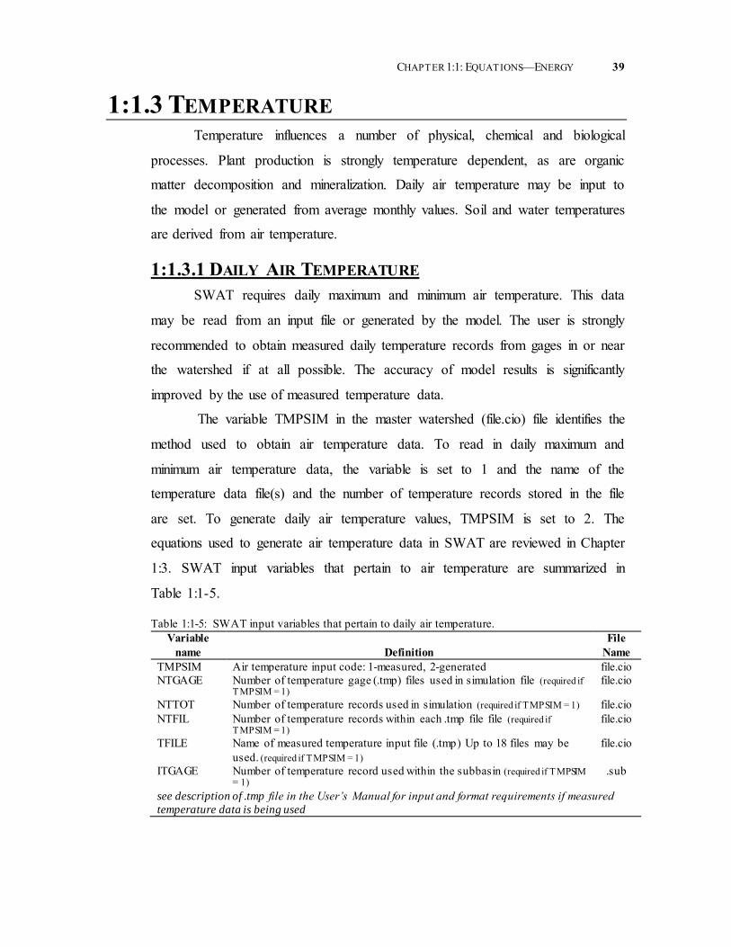
Table 1:1-5: SWAT input variables that pertain to daily air temperature. Variable
name
Definition File
Name TMPSIM Air temperature input code: 1-measured, 2-generated file.cio NTGAGE Number of temperature gage (.tmp) files used in simulation file (required if
TMPSIM = 1) file.cio
NTTOT Number of temperature records used in simulation (required if TMPSIM = 1) file.cio NTFIL Number of temperature records within each .tmp file file (required if
TMPSIM = 1) file.cio
TFILE Name of measured temperature input file (.tmp) Up to 18 files may be used. (required if TMPSIM = 1)
file.cio
ITGAGE Number of temperature record used within the subbasin (required if TMPSIM = 1)
.sub
see description of .tmp file in the User’s Manual for input and format requirements if measured
temperature data is being used

40 SWAT THEORETICAL DOCUMENTATION, VERSION 2009
1:1.3.2 HOURLY AIR TEMPERATURE
Air temperature data are usually provided in the form of daily maximum
and minimum temperature. A reasonable approximation for converting these to
hourly temperatures is to assume a sinusoidal interpolation function between the
minimum and maximum daily temperatures. The maximum daily temperature is
assumed to occur at 1500 hours and the minimum daily temperature at 300 hours
(Campbell, 1985). The temperature for the hour is then calculated with the
equation:
152618.0cos
2
hr
TTTT mnmx
avhr 1:1.3.1
where Thr is the air temperature during hour hr of the day (C), avT is the average
temperature on the day (C), Tmx is the daily maximum temperature (C), and Tmn
is the daily minimum temperature (C).
Table 1:1-6: SWAT input variables that pertain to hourly air temperature. Variable
name
Definition File
Name MAX TEMP Tmx: Daily maximum temperature (C) .tmp MIN TEMP Tmn: Daily minimum temperature (C) .tmp
1:1.3.3 SOIL TEMPERATURE Soil temperature will fluctuate due to seasonal and diurnal variations in
temperature at the surface. Figure 1:1-2 plots air temperature and soil temperature
at 5 cm and 300 cm below bare soil at College Station, Texas.
Figure 1:1-2: Four-year average air and soil temperature at College Station, Texas.

CHAPTER 1:1: EQUATIONS—ENERGY 41
This figure illustrates several important attributes of temperature variation
in the soil. First, the annual variation in soil temperature follows a sinusoidal
function. Second, the fluctuation in temperature during the year (the amplitude of
the sine wave) decreases with depth until, at some depth in the soil, the
temperature remains constant throughout the year. Finally, the timing of
maximum and minimum temperatures varies with depth. Note in the above graph
that there is a three month difference between the recording of the minimum
temperature at the surface (January) and the minimum temperature at 300 cm
(March).
Carslaw and Jaeger (1959) developed an equation to quantify the seasonal
variation in temperature:
ddzdddzATdzT ntmpsurfAAnsoil /sin/exp, 1:1.3.2
where Tsoil(z,dn) is the soil temperature (C) at depth z (mm) and day of the year
dn, AAT is the average annual soil temperature (C), Asurf is the amplitude of the
surface fluctuations (C), dd is the damping depth (mm), and tmp is the angular
frequency. When z = 0 (soil surface), equation 1:1.3.2 reduces to
ntmpsurfAAnsoil dATdT sin,0 . As z , equation 1:1.3.2 becomes
AAnsoil TdT , .
In order to calculate values for some of the variables in this equation, the
heat capacity and thermal conductivity of the soil must be known. These are
properties not commonly measured in soils and attempts at estimating values from
other soil properties have not proven very effective. Consequently, an equation
has been adopted in SWAT that calculates the temperature in the soil as a function
of the previous day’s soil temperature, the average annual air temperature, the
current day’s soil surface temperature, and the depth in the profile.
The equation used to calculate daily average soil temperature at the center
of each layer is:
ssurfssurfAAairnsoilnsoil TTTdfz,dTz,dT 0.11 1:1.3.3

42 SWAT THEORETICAL DOCUMENTATION, VERSION 2009
where Tsoil(z,dn) is the soil temperature (C) at depth z (mm) and day of the year
dn, is the lag coefficient (ranging from 0.0 to 1.0) that controls the influence of
the previous day’s temperature on the current day’s temperature, Tsoil(z,dn-1) is the
soil temperature (C) in the layer from the previous day, df is the depth factor that
quantifies the influence of depth below surface on soil temperature, AAairT is the
average annual air temperature (C), and Tssurf is the soil surface temperature on
the day. SWAT sets the lag coefficient, , to 0.80. The soil temperature from the
previous day is known and the average annual air temperature is calculated from
the long-term monthly maximum and minimum temperatures reported in the
weather generator input (.wgn) file. This leaves the depth factor, df, and the soil
surface temperature, Tssurf, to be defined.
The depth factor is calculated using the equation:
zdzd
zddf
078.2867.0exp 1:1.3.4
where zd is the ratio of the depth at the center of the soil layer to the damping
depth:
dd
zzd 1:1.3.5
where z is the depth at the center of the soil layer (mm) and dd is the damping
depth (mm).
From the previous three equations (1:1.3.3, 1:1.3.4 and 1:1.3.5) one can
see that at depths close to the soil surface, the soil temperature is a function of the
soil surface temperature. As the depth increases, soil temperature is increasingly
influenced by the average annual air temperature, until at the damping depth, the
soil temperature is within 5% of AAairT .
The damping depth, dd, is calculated daily and is a function of the
maximum damping depth, bulk density and soil water. The maximum damping
depth, ddmax, is calculated:
bb
bdd
63.5exp68625001000max
1:1.3.6

CHAPTER 1:1: EQUATIONS—ENERGY 43
where ddmax is the maximum damping depth (mm), and b is the soil bulk density
(Mg/m3).
The impact of soil water content on the damping depth is incorporated via
a scaling factor,, that is calculated with the equation:
totb z
SW
144.0356.0 1:1.3.7
where SW is the amount of water in the soil profile expressed as depth of water in
the profile (mm H2O), b is the soil bulk density (Mg/m3), and ztot is the depth
from the soil surface to the bottom of the soil profile (mm).
The daily value for the damping depth, dd, is calculated:
2
maxmax 1
1500lnexp
dddddd 1:1.3.8
where ddmax is the maximum damping depth (mm), and is the scaling factor for
soil water.
The soil surface temperature is a function of the previous day’s
temperature, the amount of ground cover and the temperature of the surface when
no cover is present. The temperature of a bare soil surface is calculated with the
equation:
2
mnmxsravbare
TTTT
1:1.3.9
where Tbare is the temperature of the soil surface with no cover (C), avT is the
average temperature on the day (C), Tmx is the daily maximum temperature (C),
Tmn is the daily minimum temperature (C), and sr is a radiation term. The
radiation term is calculated with the equation:
20141
day
sr
H 1:1.3.10
where Hday is the solar radiation reaching the ground on the current day (MJ m-2 d-1),
and is the albedo for the day.
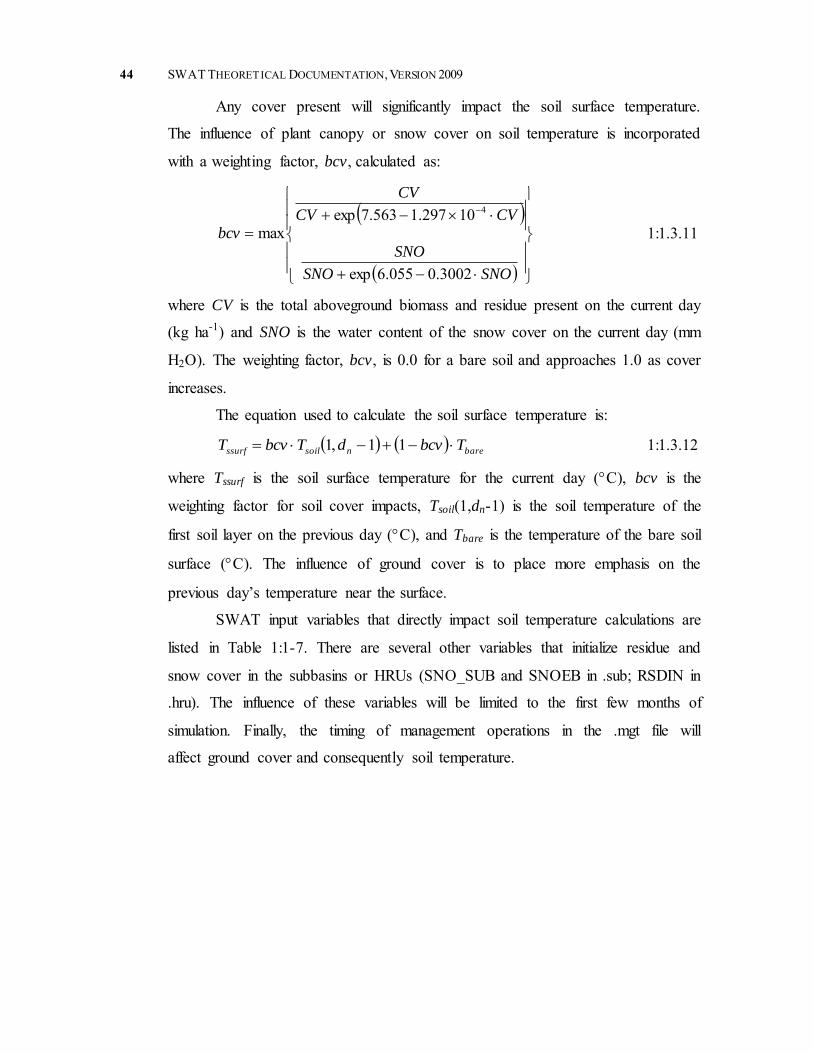
44 SWAT THEORETICAL DOCUMENTATION, VERSION 2009
Any cover present will significantly impact the soil surface temperature.
The influence of plant canopy or snow cover on soil temperature is incorporated
with a weighting factor, bcv, calculated as:
SNOSNO
SNO
CVCV
CV
bcv
3002.0055.6exp
10297.1563.7expmax
4
1:1.3.11
where CV is the total aboveground biomass and residue present on the current day
(kg ha-1) and SNO is the water content of the snow cover on the current day (mm
H2O). The weighting factor, bcv, is 0.0 for a bare soil and approaches 1.0 as cover
increases.
The equation used to calculate the soil surface temperature is:
barensoilssurf TbcvdTbcvT 11,1 1:1.3.12
where Tssurf is the soil surface temperature for the current day (C), bcv is the
weighting factor for soil cover impacts, Tsoil(1,dn-1) is the soil temperature of the
first soil layer on the previous day (C), and Tbare is the temperature of the bare soil
surface (C). The influence of ground cover is to place more emphasis on the
previous day’s temperature near the surface.
SWAT input variables that directly impact soil temperature calculations are
listed in Table 1:1-7. There are several other variables that initialize residue and
snow cover in the subbasins or HRUs (SNO_SUB and SNOEB in .sub; RSDIN in
.hru). The influence of these variables will be limited to the first few months of
simulation. Finally, the timing of management operations in the .mgt file will
affect ground cover and consequently soil temperature.

CHAPTER 1:1: EQUATIONS—ENERGY 45
Table 1:1-7: SWAT input variables that pertain to soil temperature.
Variable name
Definition
File Name
TMPMX Average maximum air temperature for month (C) .wgn TMPMN Average minimum air temperature for month (C) .wgn SOL_Z z: Depth from soil surface to bottom of layer (mm) .sol SOL_BD b: Moist bulk density (Mg m-3 or g cm-3) .sol SOL_ALB Moist soil albedo. .sol MAX TEMP Tmx: Daily maximum temperature (C) .tmp MIN TEMP Tmn: Daily minimum temperature (C) .tmp
1:1.3.4 WATER TEMPERATURE Water temperature is required to model in-stream biological and water
quality processes. SWAT uses an equation developed by Stefan and Preud’homme
(1993) to calculate average daily water temperature for a well-mixed stream:
avwater TT 75.00.5 1:1.3.13
where Twater is the water temperature for the day (C), and avT is the average air
temperature on the day (C).
Due to thermal inertia of the water, the response of water temperature to a
change in air temperature is dampened and delayed. When water and air
temperature are plotted for a stream or river, the peaks in the water temperature
plots usually lag 3-7 hours behind the peaks in air temperature. As the depth of the
river increases, the lag time can increase beyond this typical interval. For very
large rivers, the lag time can extend up to a week. Equation 1:1.3.13 assumes that
the lag time between air and water temperatures is less than 1 day.
In addition to air temperature, water temperature is influenced by solar
radiation, relative humidity, wind speed, water depth, ground water inflow,
artificial heat inputs, thermal conductivity of the sediments and the presence of
impoundments along the stream network. SWAT assumes that the impact of these
other variables on water temperature is not significant.
Table 1:1-8: SWAT input variables that pertain to water temperature. Variable
name
Definition File
Name MAX TEMP Tmx: Daily maximum temperature (C) .tmp MIN TEMP Tmn: Daily minimum temperature (C) .tmp
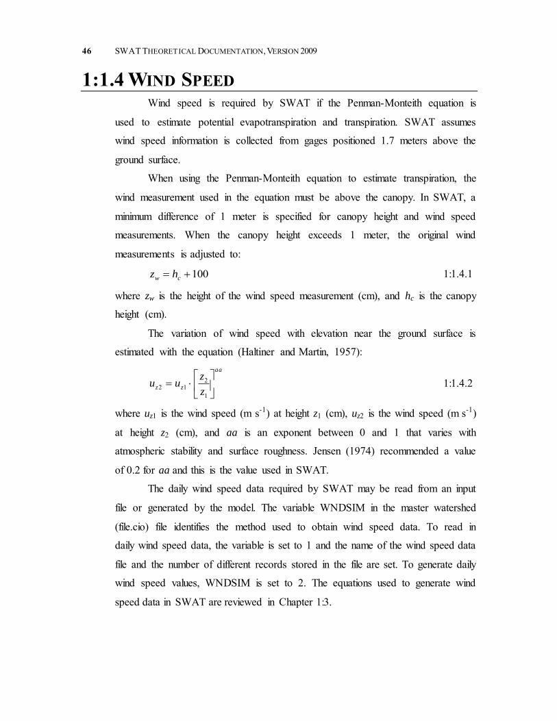
46 SWAT THEORETICAL DOCUMENTATION, VERSION 2009
1:1.4 WIND SPEED Wind speed is required by SWAT if the Penman-Monteith equation is
used to estimate potential evapotranspiration and transpiration. SWAT assumes
wind speed information is collected from gages positioned 1.7 meters above the
ground surface.
When using the Penman-Monteith equation to estimate transpiration, the
wind measurement used in the equation must be above the canopy. In SWAT, a
minimum difference of 1 meter is specified for canopy height and wind speed
measurements. When the canopy height exceeds 1 meter, the original wind
measurements is adjusted to:
100 cw hz 1:1.4.1
where zw is the height of the wind speed measurement (cm), and hc is the canopy
height (cm).
The variation of wind speed with elevation near the ground surface is
estimated with the equation (Haltiner and Martin, 1957):
aa
zzz
zuu
1
212 1:1.4.2
where uz1 is the wind speed (m s-1) at height z1 (cm), uz2 is the wind speed (m s-1)
at height z2 (cm), and aa is an exponent between 0 and 1 that varies with
atmospheric stability and surface roughness. Jensen (1974) recommended a value
of 0.2 for aa and this is the value used in SWAT.
The daily wind speed data required by SWAT may be read from an input
file or generated by the model. The variable WNDSIM in the master watershed
(file.cio) file identifies the method used to obtain wind speed data. To read in
daily wind speed data, the variable is set to 1 and the name of the wind speed data
file and the number of different records stored in the file are set. To generate daily
wind speed values, WNDSIM is set to 2. The equations used to generate wind
speed data in SWAT are reviewed in Chapter 1:3.

CHAPTER 1:1: EQUATIONS—ENERGY 47
Table 1:1-9: SWAT input variables used in wind speed calculations. Variable
name
Definition File
Name WNDSIM Wind speed input code: 1-measured, 2-generated file.cio NWTOT Number of wind speed records within the .wnd file (required if WNDSIM = 1) file.cio WNDFILE Name of measured wind speed input file (.wnd) (required if WNDSIM = 1) file.cio IWGAGE Number of wind speed record used within the subbasin (required if WNDSIM
= 1) .sub
see description of .wnd file in the User’s Manual for input and format requirements if measured
daily wind speed data is being used
1:1.5 NOMENCLATURE Asurf Amplitude of the surface fluctuations in soil temperature (C) AU Astronomical unit (1 AU = 1.496 x 10⁸ km) CV Total aboveground biomass and residue present on current day (kg ha-1) E0 Eccentricity correction factor of earth (r0/r)2 H0 Extraterrestrial daily irradiation (MJ m-2 d-1) Hb Net outgoing long-wave radiation (MJ m-2 d-1) Hday Solar radiation reaching ground on current day of simulation (MJ m-2 d-1) HL Long-wave radiation (MJ m-2 d-1) HMX Maximum possible solar radiation (MJ m-2 d-1) Hnet Net radiation on day (MJ m-2 d-1) HR Radiant energy (MJ m-2 d-1) Ifrac Fraction of daily solar radiation falling during specific hour on current day of
simulation Ihr Solar radiation reaching ground during specific hour on current day of simulation
(MJ m-2 h-1) ISC Solar constant (4.921 MJ m-2 h-1) I0 Extraterrestrial daily irradiance incident on a horizontal surface (MJ m-2 h-1) I0n Extraterrestrial daily irradiance incident on a normal surface (MJ m-2 h-1) SNO Water content of snow cover on current day (mm H2O) SW Amount of water in soil profile (mm H2O) Tbare Temperature of soil surface with no cover (C) TDL Daylength (h) Thr Air temperature during hour (C) TK Mean air temperature in Kelvin (273.15 + C) Tmn Minimum air temperature for day (C) Tmx Maximum air temperature for day (C) Tsoil Soil temperature (C) Tssurf Soil surface temperature (C) TSR Time of sunrise in solar day (h) TSS Time of sunset in solar day (h) Twater Average daily water temperature (C)
AAT Average annual soil temperature (C)

48 SWAT THEORETICAL DOCUMENTATION, VERSION 2009
AAairT Average annual air temperature (C) avT Average air temperature for day (C)
a Constant in equation used to calculate the cloud cover adjustment factor a1 Constant in equation used to calculate net emissivity aa Exponent between 0 and 1 that varies with atmospheric stability and surface
roughness that is used in calculating wind speed at different heights
b Constant in equation used to calculate the cloud cover adjustment factor b1 Constant in equation used to calculate net emissivity
bcv weighting factor for impact of ground cover on soil surface temperature covsol Soil cover index for albedo determination dn Day number of year, 1 on January 1 and 365 on December 31 dd Damping depth (mm) ddmax Maximum damping depth (mm) df Depth factor used in soil temperature calculations e Vapor pressure (actual) on a given day (kPa) fcld Factor to adjust for cloud cover in net long-wave radiation calculation
hc Canopy height (cm) hr Hour of day (1-24) r Actual earth-sun distance (AU) r0 Mean earth-sun distance, 1 AU t Number of hours before (+) or after (-) solar noon ti Solar time at the midpoint of the hour i uz1 Wind speed (m s-1) at height z1 (cm) uz2 Wind speed (m s-1) at height z2 (cm) z Depth below soil surface (mm) z1 Height of wind speed measurement (cm) z2 Height of wind speed measurement (cm) ztot Depth to bottom of soil profile (mm) zw Height of the wind speed measurement (cm) zd Ratio of depth in soil to damping depth Short-wave reflectance or albedo plant Plant albedo (set at 0.23) soil Soil albedo δ Solar declination (radians) Emissivity Net emittance a Atmospheric emittance sr Radiation term for bare soil surface temperature calculation vs Vegetative or soil emittance Lag coefficient that controls influence of previous day’s temperature on current
days temperature Stefan-Boltzmann constant (4.903 10-9 MJ m-2 K-4 d-1) θz Zenith angle (radians)

CHAPTER 1:1: EQUATIONS—ENERGY 49
Latitude in radians b Soil bulk density (Mg m-3) Scaling factor for impact of soil water on damping depth Angular velocity of the earth's rotation (0.2618 radians h-1) tmp Angular frequency in soil temperature variation
1:1.6 REFERENCES
Brunt, D. 1932. Notes on radiation in the atmosphere. Quart. J. Roy. Meteorol. Soc. 58: 389-418.
Campbell, G.S. 1985. Soil physics with BASIC: transport models for soil-plant systems. Elsevier, Amsterdam.
Carslaw, H.S. and J.C. Jaeger. 1959. Conduction of heat in solids. Oxford University Press, London.
Doorenbos, J. and W.O. Pruitt. 1977. Guidelines for predicting crop water requirements. FAO Irrig. and Drain. Paper No. 24, 2nd ed. FAO, Rome.
Duffie, J.A. and W.A. Beckman. 1980. Solar engineering of thermal processes. Wiley, N.Y.
Haltiner, G.J. and F.L. Martin. 1957. Dynamical and physical meteorology. McGraw-Hill, New York.
Iqbal, M. 1983. An introduction to solar radiation. Academic Press, N.Y. Jensen, M.E. (ed.) 1974. Consumptive use of water and irrigation water
requirements. Rep. Tech. Com. on Irrig. Water Requirements, Irrig. and Drain. Div., ASCE.
Jensen, M.E., R.D. Burman, and R.G. Allen (ed). 1990. Evapotranspiration and irrigation water requirements. ASCE Manuals and Reports on Engineering Practice No. 70, ASCE, N.Y.
Perrin de Brichambaut, Chr. 1975. Cahiers A.F.E.D.E.S., supplément au no 1. Editions Européennes Thermique et Industrie, Paris.
Stefan, H.G. and E.B. Preud’homme. 1993. Stream temperature estimation from air temperature. Water Resources Bulletin 29(1): 27-45.
Wright, J.L. and M.E. Jensen. 1972. Peak water requirements of crops in Southern Idaho. J. Irrig. and Drain. Div., ASCE, 96(IR1):193-201.

50 SWAT THEORETICAL DOCUMENTATION, VERSION 2009
51
SECTION 1 CHAPTER 2
EQUATIONS:
ATMOSPHERIC WATER
Precipitation is the mechanism by which water enters the land phase of the
hydrologic cycle. Because precipitation controls the water balance, it is critical
that the amount and distribution of precipitation in space and time is accurately
simulated by the model.

52 SWAT THEORET ICAL DOCUMENTATION, VERSION 2009
52
1:2.1 PRECIPITATION
The precipitation reaching the earth's surface on a given day, Rday, may be
read from an input file or generated by the model. Users are strongly
recommended to incorporate measured precipitation into their simulations any
time the data is available. The ability of SWAT to reproduce observed stream
hydrographs is greatly improved by the use of measured precipitation data.
Unfortunately, even with the use of measured precipitation the model user
can expect some error due to inaccuracy in precipitation data. Measurement of
precipitation at individual gages is subject to error from a number of causes and
additional error is introduced when regional precipitation is estimated from point
values. Typically, total or average areal precipitation estimates for periods of a
year or longer have relative uncertainties of 10% (Winter, 1981).
Point measurements of precipitation generally capture only a fraction of
the true precipitation. The inability of a gage to capture a true reading is primarily
caused by wind eddies created by the gage. These wind eddies reduce the catch of
the smaller raindrops and snowflakes. Larson and Peck (1974) found that
deficiencies of 10% for rain and 30% for snow are common for gages projecting
above the ground surface that are not designed to shield wind effects. Even when
the gage is designed to shield for wind effects, this source of error will not be
eliminated. For an in-depth discussion of this and other sources of error as well as
methods for dealing with the error, please refer to Dingman (1994).
The variable PCPSIM in the master watershed file (file.cio) identifies the
method used to obtain precipitation data. To read in precipitation data, the variable
is set to 1 and the names of the precipitation data files and the number of
precipitation records stored in the files are defined. To generate precipitation
values, PCPSIM is set to 2. The equations used to generate precipitation data in
SWAT are reviewed in Chapter 1:3. SWAT input variables that pertain to
precipitation are summarized in Table 1:2-1.

CHAPTER 1:2: EQUATIONS—ATMOSPHERIC WATER
53
53
Table 1:2-1: SWAT input variables used in precipitation calculations. Variable
name
Definition File
Name PCPSIM Precipitation input code: 1-measured, 2-generated file.cio NRGAGE Number of precipitation gage files (.pcp) used (required if PCPSIM = 1) file.cio NRTOT Total number of precipitation records used in simulation (required if PCPSIM
= 1) file.cio
NRGFIL Number of precipitation records in each .pcp file (required if PCPSIM = 1) file.cio RFILE Name of measured precipitation input file(s) (.pcp) (required if PCPSIM = 1) file.cio IRGAGE Number of precipitation record used within the subbasin (required if PCPSIM
= 1) .sub
see description of .pcp file in the User’s Manual for input and format requirements if measured
daily precipitation data is being used
1:2.2 MAXIMUM HALF-HOUR RAINFALL The maximum half-hour rainfall is required by SWAT to calculate the
peak runoff rate. The maximum half-hour rainfall is reported as a fraction of the
total daily rainfall, 0.5. If sub-daily precipitation data is used in the model,
SWAT will calculate the maximum half-hour rainfall fraction directly from the
precipitation data. If daily precipitation data is used, SWAT generates a value for
0.5 using the equations summarized in Chapter 1:3.
1:2.3 WATER VAPOR
Relative humidity is required by SWAT if the Penman-Monteith or
Priestley-Taylor equation is used to estimate potential evapotranspiration. It is
also used to calculate the vapor pressure deficit on plant growth. The Penman-
Monteith equation includes terms that quantify the effect of the amount of water
vapor in the air near the evaporative surface on evaporation. Both Penman-
Monteith and Priestley-Taylor require the actual vapor pressure, which is
calculated from the relative humidity.
Relative humidity is the ratio of an air volume’s actual vapor pressure to
its saturation vapor pressure:
oh
e
eR 1:2.3.1

54 SWAT THEORET ICAL DOCUMENTATION, VERSION 2009
54
where Rh is the relative humidity on a given day, e is the actual vapor pressure on
a given day (kPa), and oe is the saturation vapor pressure on a given day (kPa).
The saturation vapor pressure is the maximum vapor pressure that is
thermodynamically stable and is a function of the air temperature. SWAT
calculates saturation vapor pressure using an equation presented by Tetens (1930)
and Murray (1967):
3.2379.11678.16exp
av
avo
T
Te 1:2.3.2
where oe is the saturation vapor pressure on a given day (kPa) and avT is the
mean daily air temperature (C). When relative humidity is known, the actual
vapor pressure can be calculated by rearranging equation 1:2.3.1:
o
h eRe 1:2.3.3
The saturation vapor pressure curve is obtained by plotting equation
1:2.3.2. The slope of the saturation vapor pressure curve can be calculated by
differentiating equation 1:2.3.2:
23.237
4098
av
o
T
e 1:2.3.4
where is the slope of the saturation vapor pressure curve (kPa C-1), oe is the
saturation vapor pressure on a given day (kPa) and avT is the mean daily air
temperature (C).
The rate of evaporation is proportional to the difference between the vapor
pressure of the surface layer and the vapor pressure of the overlying air. This
difference is termed the vapor pressure deficit:
eevpd o 1:2.3.5
where vpd is the vapor pressure deficit (kPa), oe is the saturation vapor pressure
on a given day (kPa), and e is the actual vapor pressure on a given day (kPa). The
greater the value of vpd the higher the rate of evaporation.
The latent heat of vaporization, , is the quantity of heat energy that must
be absorbed to break the hydrogen bonds between water molecules in the liquid

CHAPTER 1:2: EQUATIONS—ATMOSPHERIC WATER
55
55
state to convert them to gas. The latent heat of vaporization is a function of
temperature and can be calculated with the equation (Harrison, 1963):
avT 310361.2501.2 1:2.3.6
where is the latent heat of vaporization (MJ kg-1) and avT is the mean daily air
temperature (C).
Evaporation involves the exchange of both latent heat and sensible heat
between the evaporating body and the air. The psychrometric constant, ,
represents a balance between the sensible heat gained from air flowing past a wet
bulb thermometer and the sensible heat converted to latent heat (Brunt, 1952) and
is calculated:
622.0Pcp 1:2.3.7
where is the psychrometric constant (kPa C-1), cp is the specific heat of moist
air at constant pressure (1.013 10-3 MJ kg-1 C-1), P is the atmospheric pressure
(kPa), and is the latent heat of vaporization (MJ kg-1).
Calculation of the psychrometric constant requires a value for atmospheric
pressure. SWAT estimates atmospheric pressure using an equation developed by
Doorenbos and Pruitt (1977) from mean barometric pressure data at a number of
East African sites:
2610544.001152.03.101 ELELP 1:2.3.8
where P is the atmospheric pressure (kPa) and EL is the elevation (m).
The daily relative humidity data required by SWAT may be read from an
input file or generated by the model. The variable RHSIM in the master watershed
(file.cio) file identifies the method used to obtain relative humidity data. To read
in daily relative humidity data, the variable is set to 1 and the name of the relative
humidity data file and the number of different records stored in the file are set. To
generate daily relative humidity values, RHSIM is set to 2. The equations used to
generate relative humidity data in SWAT are reviewed in Chapter 1:3.

56 SWAT THEORET ICAL DOCUMENTATION, VERSION 2009
56
Table 1:2-2: SWAT input variables used in relative humidity calculations. Variable
name
Definition File
Name RHD Rh: daily average relative humidity .hmd TMP_MX Tmx: maximum temperature for day (C) .tmp TMP_MN Tmn: minimum temperature for day (C) .tmp SUB_ELEV EL: elevation (m) .sub RHSIM Relative humidity input code: 1-measured, 2-generated file.cio NHTOT Number of relative humidity records within the .hmd file (required if RHSIM
= 1) file.cio
RHFILE Name of measured relative humidity input file (.hmd) (required if RHSIM = 1)
file.cio
IHGAGE Number of relative humidity record used within the subbasin (required if RHSIM = 1)
.sub
see description of .hmd file in the User’s Manual for input and format requirements if measured
relative humidity data is being used
1:2.4 SNOW COVER SWAT classifies precipitation as rain or freezing rain/snow by the mean
daily air temperature. The boundary temperature, Ts-r, used to categorize
precipitation as rain or snow is defined by the user. If the mean daily air
temperature is less than the boundary temperature, then the precipitation within
the HRU is classified as snow and the water equivalent of the snow precipitation
is added to the snow pack.
Snowfall is stored at the ground surface in the form of a snow pack. The
amount of water stored in the snow pack is reported as a snow water equivalent.
The snow pack will increase with additional snowfall or decrease with snow melt
or sublimation. The mass balance for the snow pack is:
mltsubday SNOERSNOSNO 1:2.4.1
where SNO is the water content of the snow pack on a given day (mm H2O), Rday
is the amount of precipitation on a given day (added only if rsav TT ) (mm
H2O), Esub is the amount of sublimation on a given day (mm H2O), and SNOmlt is
the amount of snow melt on a given day (mm H2O). The amount of snow is
expressed as depth over the total HRU area.
Due to variables such as drifting, shading and topography, the snow pack
in a subbasin will rarely be uniformly distributed over the total area. This results

CHAPTER 1:2: EQUATIONS—ATMOSPHERIC WATER
57
57
in a fraction of the subbasin area that is bare of snow. This fraction must be
quantified to accurately compute snow melt in the subbasin.
The factors that contribute to variable snow coverage are usually similar
from year to year, making it possible to correlate the areal coverage of snow with
the amount of snow present in the subbasin at a given time. This correlation is
expressed as an areal depletion curve, which is used to describe the seasonal
growth and recession of the snow pack as a function of the amount of snow
present in the subbasin (Anderson, 1976).
The areal depletion curve requires a threshold depth of snow, SNO100, to
be defined above which there will always be 100% cover. The threshold depth
will depend on factors such as vegetation distribution, wind loading of snow,
wind scouring of snow, interception and aspect, and will be unique to the
watershed of interest.
The areal depletion curve is based on a natural logarithm. The areal
depletion curve equation is: 1
10021
100100cov exp
SNO
SNOcovcov
SNO
SNO
SNO
SNOsno 1:2.4.2
where snocov is the fraction of the HRU area covered by snow, SNO is the water
content of the snow pack on a given day (mm H2O), SNO100 is the threshold depth
of snow at 100% coverage (mm H2O), cov1 and cov2 are coefficients that define
the shape of the curve. The values used for cov1 and cov2 are determined by
solving equation 1:2.4.2 using two known points: 95% coverage at 95% SNO100;
and 50% coverage at a user specified fraction of SNO100.
Example areal depletion curves for various fractions of SNO100 at 50%
coverage are shown in the following figures.

58 SWAT THEORET ICAL DOCUMENTATION, VERSION 2009
58
Figure 1:2-1:10% SNO100 = 50% coverage Figure 1:2-2: 30% SNO100 = 50% coverage
Figure 1:2-3: 50% SNO100 = 50% coverage Figure 1:2-4: 70% SNO100 = 50% coverage
Figure 1:2-5: 90% SNO100 = 50% coverage It is important to remember that once the volume of water held in the snow
pack exceeds SNO100 the depth of snow over the HRU is assumed to be uniform,
i.e. snocov = 1.0. The areal depletion curve affects snow melt only when the snow
0
0.1
0.2
0.3
0.4
0.5
0.6
0.7
0.8
0.9
1
0 0.1 0.2 0.3 0.4 0.5 0.6 0.7 0.8 0.9 1
Fra
cti
on
are
al co
vera
ge
Snow volume (fraction of SNO100)
0
0.1
0.2
0.3
0.4
0.5
0.6
0.7
0.8
0.9
1
0 0.1 0.2 0.3 0.4 0.5 0.6 0.7 0.8 0.9 1
Fra
cti
on
are
al co
vera
ge
Snow volume (fraction of SNO100)
0
0.1
0.2
0.3
0.4
0.5
0.6
0.7
0.8
0.9
1
0 0.1 0.2 0.3 0.4 0.5 0.6 0.7 0.8 0.9 1
Fra
cti
on
are
al
co
ve
rag
e
Snow v olume (fraction of SNO100)
0
0.1
0.2
0.3
0.4
0.5
0.6
0.7
0.8
0.9
1
0 0.1 0.2 0.3 0.4 0.5 0.6 0.7 0.8 0.9 1
Fra
cti
on
are
al
co
ve
rag
e
Snow v olume (fraction of SNO100)
0
0.1
0.2
0.3
0.4
0.5
0.6
0.7
0.8
0.9
1
0 0.1 0.2 0.3 0.4 0.5 0.6 0.7 0.8 0.9 1
Fra
cti
on
are
al
co
ve
rag
e
Snow v olume (fraction of SNO100)

CHAPTER 1:2: EQUATIONS—ATMOSPHERIC WATER
59
59
pack water content is between 0.0 and SNO100. Consequently if SNO100 is set to a
very small value, the impact of the areal depletion curve on snow melt will be
minimal. As the value for SNO100 increases, the influence of the areal depletion
curve will assume more importance in snow melt processes.
Table 1:2-3: SWAT input variables used in snow cover calculations. Variable
name
Definition File
Name SFTMP Ts-r: Mean air temperature at which precipitation is equally likely to be
rain as snow/freezing rain (C) .bsn
SNOCOVMX SNO100: Threshold depth of snow, above which there is 100% cover .bsn SNO50COV Fraction of SNOCOVMX that provides 50% cover .bsn SNO_SUB Initial snow water content in subbasin (mm H2O) .sub SNOEB Initial snow water content in subbasin elevation band (mm H2O) .sub
1:2.5 SNOW MELT
Snow melt is controlled by the air and snow pack temperature, the melting
rate, and the areal coverage of snow.
Snow melt is included with rainfall in the calculations of runoff and
percolation. When SWAT calculates erosion, the rainfall energy of the snow melt
fraction of the water is set to zero. The water released from snow melt is assumed
to be evenly distributed over the 24 hours of the day.
1:2.5.1 SNOW PACK TEMPERATURE
The snow pack temperature is a function of the mean daily temperature
during the preceding days and varies as a dampened function of air temperature
(Anderson, 1976). The influence of the previous day’s snow pack temperature on
the current day’s snow pack temperature is controlled by a lagging factor, sno .
The lagging factor inherently accounts for snow pack density, snow pack depth,
exposure and other factors affecting snow pack temperature. The equation used to
calculate the snow pack temperature is:
snoavsnodsnowdsnow TTTnn
11 1:2.5.1
where ndsnowT is the snow pack temperature on a given day (C), 1ndsnowT is the
snow pack temperature on the previous day (C), sno is the snow temperature lag

60 SWAT THEORET ICAL DOCUMENTATION, VERSION 2009
60
factor, and avT is the mean air temperature on the current day (C). As sno
approaches 1.0, the mean air temperature on the current day exerts an increasingly
greater influence on the snow pack temperature and the snow pack temperature
from the previous day exerts less and less influence.
The snow pack will not melt until the snow pack temperature exceeds a
threshold value, Tmlt. This threshold value is specified by the user.
1:2.5.2 SNOW MELT EQUATION
The snow melt in SWAT is calculated as a linear function of the
difference between the average snow pack-maximum air temperature and the base
or threshold temperature for snow melt:
mlt
mxsnowmltmlt T
TTsnobSNO
2cov 1:2.5.2
where SNOmlt is the amount of snow melt on a given day (mm H2O), bmlt is the
melt factor for the day (mm H2O/day-C), snocov is the fraction of the HRU area
covered by snow, snowT is the snow pack temperature on a given day (C), Tmx is
the maximum air temperature on a given day (C), and Tmlt is the base temperature
above which snow melt is allowed (C).
The melt factor is allowed a seasonal variation with maximum and
minimum values occurring on summer and winter solstices:
81
3652sin
22126126
nmltmltmltmlt
mlt dbbbb
b 1:2.5.3
where bmlt is the melt factor for the day (mm H2O/day-C), bmlt6 is the melt factor
for June 21 (mm H2O/day-C), bmlt12 is the melt factor for December 21 (mm
H2O/day-C), and dn is the day number of the year.
In rural areas, the melt factor will vary from 1.4 to 6.9 mm H2O/day-C
(Huber and Dickinson, 1988). In urban areas, values will fall in the higher end of
the range due to compression of the snow pack by vehicles, pedestrians, etc.
Urban snow melt studies in Sweden (Bengston, 1981; Westerstrom, 1981)
reported melt factors ranging from 3.0 to 8.0 mm H2O/day-C. Studies of snow

CHAPTER 1:2: EQUATIONS—ATMOSPHERIC WATER
61
61
melt on asphalt (Westerstrom, 1984) gave melt factors of 1.7 to 6.5 mm H2O/day-
C.
Table 1:2-4: SWAT input variables used in snow melt calculations. Variable
name
Definition File
Name TIMP
sno : Snow temperature lag factor .bsn
SMTMP Tmlt: Threshold temperature for snow melt (C) .bsn SMFMX bmlt6: Melt factor on June 21 (mm H2O/day-C) .bsn SMFMN bmlt12: Melt factor on December 21 (mm H2O/day-C) .bsn
1:2.6 NOMENCLATURE Esub Amount of sublimation on a given day (mm H2O) EL Elevation (m) P Atmospheric pressure (kPa) Rday Amount of rainfall on a given day (mm H2O) Rh Average relative humidity for the day SNO Water content of snow cover on current day (mm H2O) SNO100Amount of snow above which there is 100% cover (mm H2O) SNOmlt Amount of snow melt on a given day (mm H2O) Tmlt Threshold temperature for snow melt (C) Tmx Maximum air temperature for day (C) Ts-r Rain/snow boundary temperature (C)
snowT Snow pack temperature on a given day (C)
avT Average air temperature for day (C) bmlt Melt factor for the day (mm H2O/day-C) bmlt6 Melt factor for June 21 (mm H2O/day-C) bmlt12 Melt factor for December 21 (mm H2O/day-C) cp Specific heat of moist air at constant pressure (1.013 10-3 MJ kg-1 C-1) cov1 Snow cover areal depletion curve shape coefficient cov2 Snow cover areal depletion curve shape coefficient dn Day number of year, 1 on January 1 and 365 on December 31 e Actual vapor pressure on a given day (kPa)
oe Saturation vapor pressure on a given day (kPa) snocov Fraction of the HRU area covered by snow vpd Vapor pressure deficit (kPa) 0.5 Maximum half-hour rainfall expressed as a fraction of daily rainfall Slope of the saturation vapor pressure curve (kPa C-1) Psychrometric constant (kPa C-1) Latent heat of vaporization (MJ kg-1)

62 SWAT THEORET ICAL DOCUMENTATION, VERSION 2009
62
sno Snow temperature lag factor
1:2.7 REFERENCES
Anderson, E.A. 1976. A point energy and mass balance model of snow cover.
NOAA Technical Report NWS 19, U.S. Dept. of Commerce, National
Weather Service.
Bengston, L. 1981. Snowmelt-generated runoff in urban areas. p. 444-451. In
B.C. Yen (ed.) Urban stormwater hydraulics and hydrology: proceedings
of the Second International Conference on Urban Storm Drainage, held at
Urbana, Illinois, USA, 15-19 June 1981. Water Resources Publications,
Littleton, CO.
Brunt, D. 1952. Physical and dynamical meteorology, 2nd ed. University Press,
Cambridge.
Dingman, S.L. 1994. Physical hydrology. Prentice-Hall, Inc., Englewood Cliffs,
NJ.
Doorenbos, J. and W.O. Pruitt. 1977. Guidelines for predicting crop water
requirements. FAO Irrig. and Drain. Paper No. 24, 2nd ed. FAO, Rome.
Harrison, L.P. 1963. Fundamental concepts and definitions relating to humidity.
In A. Wexler (ed.) Humidity and moisture, Vol. 3. Reinhold Publishing
Company, N.Y.
Huber, W.C. and R.E. Dickinson. 1988. Storm water management model, version
4: user’s manual. U.S. Environmental Protection Agency, Athens, GA.
Larson, L.L., and E.L. Peck. 1974. Accuracy of precipitation measurements for
hydrologic modeling. Water Resources Research 10:857-863.
Murray, F.W. 1967. On the computation of saturation vapor pressure. J. Appl.
Meteor. 6:203-204.
Tetens, O. 1930. Uber einige meteorologische Begriffe. Z. Geophys. 6:297-309.
Westerstrom, G. 1984. Snowmelt runoff from Porson residential area, Lulea,
Sweden. p. 315-323. In Proceedings of the Third International Conference

CHAPTER 1:2: EQUATIONS—ATMOSPHERIC WATER
63
63
on Urban Storm Drainage held at Chalmers University, Goteborg,
Sweden, June 1984.
Westerstrom, G. 1981. Snowmelt runoff from urban plot. p. 452-459. In B.C. Yen
(ed.) Urban stormwater hydraulics and hydrology: proceedings of the
Second International Conference on Urban Storm Drainage, held at
Urbana, Illinois, USA, 15-19 June 1981. Water Resources Publications,
Littleton, CO.
Winter, T.C. 1981. Uncertainties in estimating the water balance of lakes. Water
Resources Bulletin 17:82-115.

64 SWAT THEORET ICAL DOCUMENTATION, VERSION 2009
64

65
SECTION 1 CHAPTER 3
EQUATIONS:
WEATHER GENERATOR
SWAT requires daily values of precipitation, maximum and minimum
temperature, solar radiation, relative humidity and wind speed. The user may
choose to read these inputs from a file or generate the values using monthly
average data summarized over a number of years.
SWAT includes the WXGEN weather generator model (Sharpley and
Williams, 1990) to generate climatic data or to fill in gaps in measured records.
This weather generator was developed for the contiguous U.S. If the user prefers a
different weather generator, daily input values for the different weather parameters
may be generated with an alternative model and formatted for input to SWAT.
The occurrence of rain on a given day has a major impact on relative
humidity, temperature and solar radiation for the day. The weather generator first
independently generates precipitation for the day. Once the total amount of rainfall
for the day is generated, the distribution of rainfall within the day is computed if

66 SWAT THEORETICAL DOCUMENTATION, VERSION 2009
66
the Green & Ampt method is used for infiltration. Maximum temperature,
minimum temperature, solar radiation and relative humidity are then generated
based on the presence or absence of rain for the day. Finally, wind speed is
generated independently.
1:3.1 PRECIPITATION
The daily precipitation generator is a Markov chain-skewed (Nicks, 1974)
or Markov chain-exponential model (Williams, 1995). A first-order Markov chain
is used to define the day as wet or dry. When a wet day is generated, a skewed
distribution or exponential distribution is used to generate the precipitation
amount. Table 1:3.1 lists SWAT input variables that are used in the precipitation
generator.
1:3.1.1 OCCURRENCE OF WET OR DRY DAY With the first-order Markov-chain model, the probability of rain on a given
day is conditioned on the wet or dry status of the previous day. A wet day is
defined as a day with 0.1 mm of rain or more.
The user is required to input the probability of a wet day on day i given a
wet day on day i – 1, Pi(W/W), and the probability of a wet day on day i given a
dry day on day i – 1, Pi(W/D), for each month of the year. From these inputs the
remaining transition probabilities can be derived:
WWPWDP ii 1 1:3.1.1
DWPDDP ii 1 1:3.1.2
where Pi(D/W) is the probability of a dry day on day i given a wet day on day i – 1
and Pi(D/D) is the probability of a dry day on day i given a dry day on day i – 1.
To define a day as wet or dry, SWAT generates a random number between
0.0 and 1.0. This random number is compared to the appropriate wet-dry
probability, Pi(W/W) or Pi(W/D). If the random number is equal to or less than the
wet-dry probability, the day is defined as wet. If the random number is greater than
the wet-dry probability, the day is defined as dry.

CHAPTER 1:3: EQUATIONS—WEATHER GENERATOR
67
67
1:3.1.2 AMOUNT OF PRECIPITATION Numerous probability distribution functions have been used to describe the
distribution of rainfall amounts. SWAT provides the user with two options: a
skewed distribution and an exponential distribution.
The skewed distribution was proposed by Nicks (1974) and is based on a
skewed distribution used by Fiering (1967) to generate representative streamflow.
The equation used to calculate the amount of precipitation on a wet day is:
mon
monmonday
monmondayg
ggSND
R
1166
2
3
1:3.1.3
where Rday is the amount of rainfall on a given day (mm H2O), mon is the mean
daily rainfall (mm H2O) for the month, mon is the standard deviation of daily
rainfall (mm H2O) for the month, SNDday is the standard normal deviate calculated
for the day, and gmon is the skew coefficient for daily precipitation in the month.
The standard normal deviate for the day is calculated:
12 ln2283.6cos rndrndSNDday 1:3.1.4
where rnd1 and rnd2 are random numbers between 0.0 and 1.0.
The exponential distribution is provided as an alternative to the skewed
distribution. This distribution requires fewer inputs and is most commonly used in
areas where limited data on precipitation events is available. Daily precipitation is
calculated with the exponential distribution using the equation:
exp1ln r
monday rndR 1:3.1.5
where Rday is the amount of rainfall on a given day (mm H2O), mon is the mean
daily rainfall (mm H2O) for the month, rnd1 is a random number between 0.0 and
1.0, and rexp is an exponent that should be set between 1.0 and 2.0. As the value of
rexp is increased, the number of extreme rainfall events during the year will
increase. Testing of this equation at locations across the U.S. have shown that a
value of 1.3 gives satisfactory results.

68 SWAT THEORETICAL DOCUMENTATION, VERSION 2009
68
Table 1:3-1: SWAT input variables that pertain to generation of precipitation. Variable
name
Definition File
Name PCPSIM Precipitation input code: 1-measured, 2-generated file.cio PR_W(1,mon) Pi(W/D): probability of a wet day following a dry day in month .wgn PR_W(2,mon) Pi(W/W): probability of a wet day following a wet day in month .wgn IDIST Rainfall distribution code: 0-skewed, 1-exponential file.cio REXP rexp: value of exponent (required if IDIST = 1) file.cio PCPMM(mon) average amount of precipitation falling in month (mm H2O) .wgn PCPD(mon) average number of days of precipitation in month .wgn (mon = PCPMM / PCPD) PCPSTD(mon) mon: standard deviation for daily precipitation in month (mm H2O) .wgn PCPSKW(mon) gmon: skew coefficient for daily precipitation in month .wgn
1:3.2 MAXIMUM HALF-HOUR RAINFALL Maximum half-hour rainfall is required by SWAT to calculate the peak
flow rate for runoff. When daily precipitation data are used by the model, the
maximum half-hour rainfall may be calculated from a triangular distribution using
monthly maximum half-hour rainfall data or the user may choose to use the
monthly maximum half-hour rainfall for all days in the month. The maximum half-
hour rainfall is calculated only on days where surface runoff has been generated.
1:3.2.1 MONTHLY MAXIMUM HALF-HOUR RAIN For each month, users provide the maximum half-hour rain observed over
the entire period of record. These extreme values are used to calculate
representative monthly maximum half-hour rainfall fractions.
Prior to calculating the representative maximum half-hour rainfall fraction
for each month, the extreme half-hour rainfall values are smoothed by calculating
three month average values:
3)1(5.0)(5.0)1(5.0
)(5.0
monxmonxmonx
monsm
RRRR 1:3.2.1
where R0.5sm(mon) is the smoothed maximum half-hour rainfall for a given month
(mm H2O) and R0.5x is the extreme maximum half-hour rainfall for the specified
month (mm H2O). Once the smoothed maximum half-hour rainfall is known, the
representative half-hour rainfall fraction is calculated using the equation:

CHAPTER 1:3: EQUATIONS—WEATHER GENERATOR
69
69
wet
mon
monsm
mon
daysyrs
Radj
5.0lnexp1 )(5.0
5.05.0
1:3.2.2
where 0.5mon is the average half-hour rainfall fraction for the month, adj0.5 is an
adjustment factor, R0.5sm is the smoothed half-hour rainfall amount for the month
(mm H2O), mon is the mean daily rainfall (mm H2O) for the month, yrs is the
number of years of rainfall data used to obtain values for monthly extreme half-
hour rainfalls, and dayswet are the number of wet days in the month. The
adjustment factor is included to allow users to modify estimations of half-hour
rainfall fractions and peak flow rates for runoff.
1:3.2.2 DAILY MAXIMUM HALF-HOUR RAIN VALUE The user has the option of using the monthly maximum half-hour rainfall
for all days in the month or generating a daily value. The variable ISED_DET in
the basin input file (.bsn) defines which option the user prefers. The randomness of
the triangular distribution used to generated daily values can cause the maximum
half-hour rainfall value to jump around. For small plots or microwatersheds in
particular, the variability of the triangular distribution is unrealistic.
The triangular distribution used to generate the maximum half-hour rainfall
fraction requires four inputs: average monthly half-hour rainfall fraction,
maximum value for half-hour rainfall fraction allowed in month, minimum value
for half-hour rainfall fraction allowed in month, and a random number between 0.0
and 1.0.
The maximum half-hour rainfall fraction, or upper limit of the triangular
distribution, is calculated from the daily amount of rainfall with the equation:
5125exp15.0
day
UR
1:3.2.3
where 0.5U is the largest half-hour fraction that can be generated on a given day,
and Rday is the precipitation on a given day (mm H2O).

70 SWAT THEORETICAL DOCUMENTATION, VERSION 2009
70
The minimum half-hour fraction, or lower limit of the triangular
distribution, 0.5L, is set at 0.02083.
The triangular distribution uses one of two sets of equations to generate a
maximum half-hour rainfall fraction for the day. If
LU
Lmonrnd5.05.0
5.05.01
then
mean
LmonLUL
mon
rnd
5.0
5.05.05.05.05.015.0
5.05.0
1:3.2.4
If
LU
Lmonrnd5.05.0
5.05.01
then
mean
monU
LU
monUU
mon
rndrnd
5.0
5.0
5.05.0
15.015.05.05.05.0
5.05.0
11
1:3.2.5
where 0.5 is the maximum half-hour rainfall fraction for the day, 0.5mon is the
average maximum half-hour rainfall fraction for the month, rnd1 is a random
number generated by the model each day, 0.5L is the smallest half-hour rainfall
fraction that can be generated, 0.5U is the largest half-hour fraction that can be
generated, and 0.5mean is the average of 0.5L, 0.5mon, and 0.5U.
Table 1:3-2: SWAT input variables that pertain to generation of maximum half-hour rainfall. Variable name
Definition File
Name ISED_DET Code governing calculation of daily maximum half-hour rainfall: 0-
generate daily value 1-use monthly maximum half-hour rainfall value .bsn
RAINHHMX(mon) R0.5x: extreme half-hour rainfall for month (mm H2O) .wgn ADJ_PKR adj0.5: peak rate adjustment factor .bsn PCPMM(mon) average amount of precipitation falling in month (mm H2O) .wgn PCPD(mon) dayswet: average number of days of precipitation in month .wgn (mon = PCPMM / PCPD) RAIN_YRS yrs: number of years of data used to obtain values for RAINHHMX .wgn PRECIPITATION Rday: amount of rain falling on a given day (mm H2O) .pcp

CHAPTER 1:3: EQUATIONS—WEATHER GENERATOR
71
71
1:3.3 DISTRIBUTION OF RAINFALL WITHIN DAY For simulations where the timing of rainfall within the day is required, the
daily rainfall value must be partitioned into shorter time increments. The method
used in SWAT to disaggregate storm data was taken from CLIGEN (Nicks et al.,
1995).
A double exponential function is used to represent the intensity patterns
within a storm. With the double exponential distribution, rainfall intensity
exponentially increases with time to a maximum, or peak, intensity. Once the peak
intensity is reached, the rainfall intensity exponentially decreases with time until
the end of the storm.
The exponential equations governing rainfall intensity during a storm event
are:
2
1
exp
exp
TTi
TTi
Ti
peak
mx
peak
mx
durpeak
peak
TTT
TT
0 1:3.3.1
where i is the rainfall intensity at time T (mm/hr), imx is the maximum or peak
rainfall intensity during the storm (mm/hr), T is the time since the beginning of the
storm (hr), Tpeak is the time from the beginning of the storm till the peak rainfall
intensity occurs (hr), Tdur is the duration of the storm (hr), and 1 and 2 are
equation coefficients (hr).
The maximum or peak rainfall intensity during the storm is calculated
assuming the peak rainfall intensity is equivalent to the rainfall intensity used to
calculate the peak runoff rate. The equations used to calculate the intensity are
reviewed in Chapter 2:1 (section 2:1.3.3).
1:3.3.1 NORMALIZED INTENSITY DISTRIBUTION The rainfall intensity distribution given in equation 1:3.3.1 can be
normalized to eliminate units. To do this, all time values are divided, or
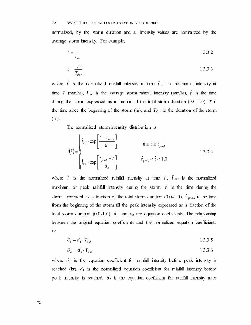
72 SWAT THEORETICAL DOCUMENTATION, VERSION 2009
72
normalized, by the storm duration and all intensity values are normalized by the
average storm intensity. For example,
avei
ii ˆ 1:3.3.2
durT
Tt ˆ 1:3.3.3
where i is the normalized rainfall intensity at time t , i is the rainfall intensity at
time T (mm/hr), iave is the average storm rainfall intensity (mm/hr), t is the time
during the storm expressed as a fraction of the total storm duration (0.0-1.0), T is
the time since the beginning of the storm (hr), and Tdur is the duration of the storm
(hr).
The normalized storm intensity distribution is
2
1
ˆˆexpˆ
ˆˆexpˆ
ˆˆ
d
tti
d
tti
ti
peak
mx
peak
mx
0.1ˆˆ
ˆˆ0
tt
tt
peak
peak
1:3.3.4
where i is the normalized rainfall intensity at time t , i mx is the normalized
maximum or peak rainfall intensity during the storm, t is the time during the
storm expressed as a fraction of the total storm duration (0.0-1.0), t peak is the time
from the beginning of the storm till the peak intensity expressed as a fraction of the
total storm duration (0.0-1.0), d1 and d2 are equation coefficients. The relationship
between the original equation coefficients and the normalized equation coefficients
is:
durTd 11 1:3.3.5
durTd 22 1:3.3.6
where 1 is the equation coefficient for rainfall intensity before peak intensity is
reached (hr), d1 is the normalized equation coefficient for rainfall intensity before
peak intensity is reached, 2 is the equation coefficient for rainfall intensity after

CHAPTER 1:3: EQUATIONS—WEATHER GENERATOR
73
73
peak intensity is reached (hr), d2 is the normalized equation coefficient for rainfall
intensity after peak intensity is reached, and Tdur is the storm duration (hr).
Values for the equation coefficients, d1 and d2, can be determined by
isolating the coefficients in equation 1:3.3.4. At t = 0.0 and at t = 1.0, 01.0ˆˆ
mxi
i.
605.4
ˆ
01.0ln
ˆ0
ˆˆ
ln
ˆˆ1
peakpeak
mx
peak tt
i
i
ttd
1:3.3.7
605.4
ˆ0.101.0ln
1ˆ
ˆˆ
ln
ˆˆ2
peakpeak
mx
peak tt
i
i
ttd
1:3.3.8
where d1 is the normalized equation coefficient for rainfall intensity before peak
intensity is reached, d2 is the normalized equation coefficient for rainfall intensity
after peak intensity is reached, t is the time during the storm expressed as a
fraction of the total storm duration (0.0-1.0), t peak is the time from the beginning
of the storm till the peak intensity expressed as a fraction of the total storm
duration (0.0-1.0), i is the normalized rainfall intensity at time t , and i mx is the
normalized maximum or peak rainfall intensity during the storm.
1:3.3.2 GENERATED TIME TO PEAK INTENSITY The normalized time to peak intensity is calculated by SWAT using a
triangular distribution. The triangular distribution used to generate the normalized
time to peak intensity requires four inputs: average time to peak intensity
expressed as a fraction of total storm duration ( peakMt ), maximum time to peak
intensity expressed as a fraction of total storm duration ( peakUt ), minimum time to
peak intensity expressed as a fraction of total storm duration ( peakLt ), and a random
number between 0.0 and 1.0.
The maximum time to peak intensity, or upper limit of the triangular
distribution, is set at 0.95. The minimum time to peak intensity, or lower limit of

74 SWAT THEORETICAL DOCUMENTATION, VERSION 2009
74
the triangular distribution is set at 0.05. The mean time to peak intensity is set at
0.25.
The triangular distribution uses one of two sets of equations to generate a
normalized peak intensity for the day. If
peakLpeakU
peakLpeakM
tt
ttrnd ˆˆ
ˆˆ1 then
meanpeak
peakLpeakMpeakLpeakUpeakL
peakMpeakt
ttttrndttt
,
5.01
ˆˆˆˆˆˆ
ˆˆ 1:3.3.9
If
peakLpeakU
peakLpeakM
tt
ttrnd ˆˆ
ˆˆ1 then
meanpeak
peakMpeakU
peakLpeakU
peakMpeakUpeakU
peakMpeakt
tt
rndtrndtttt
tt,
5.0
11
ˆ
ˆˆ1ˆ1ˆ
ˆˆˆ
ˆˆ
1:3.3.10
where t peak is the time from the beginning of the storm till the peak intensity
expressed as a fraction of the total storm duration (0.0-1.0), is the average
time to peak intensity expressed as a fraction of storm duration, rnd1 is a random
number generated by the model each day, is the minimum time to peak
intensity that can be generated, is the maximum time to peak intensity that
can be generated, and meanpeakt ,ˆ is the mean of peakLt , peakMt , and peakUt .
1:3.3.3 TOTAL RAINFALL AND DURATION The volume of rain is related to rainfall intensity by:
T
0
dTiRT 1:3.3.11
where RT is the amount of rain that has fallen at time T (mm H2O) and i is the
rainfall intensity at time T (mm/hr).
Using the definition for rainfall intensity given in equation 1:3.3.1,
equation 1:3.3.11 can be integrated to get:
peakMt
peakLt
peakUt

CHAPTER 1:3: EQUATIONS—WEATHER GENERATOR
75
75
22
11
exp1
exp1
TTiR
TTiR
R
peak
mxTpeak
peak
mxTpeak
T
durpeak
peak
TTT
TT
0 1:3.3.12
where RT is the cumulative amount of rain that has fallen at time T (mm H2O),
RTpeak is the amount of rain that has fallen at time Tpeak (mm H2O), imx is the
maximum or peak rainfall intensity during the storm (mm/hr), 1 is the equation
coefficient for rainfall intensity before peak intensity is reached (hr), 2 is the
equation coefficient for rainfall intensity after peak intensity is reached (hr), Tpeak
is the time from the beginning of the storm till the peak rainfall intensity occurs
(hr), and Tdur is the storm duration (hr). The time to peak intensity is defined as
durpeakpeak TtT ˆ 1:3.3.13
where Tpeak is the time from the beginning of the storm till the peak rainfall
intensity occurs (hr), t peak is the time from the beginning of the storm till the peak
intensity expressed as a fraction of the total storm duration (0.0-1.0), and Tdur is the
storm duration (hr). The cumulative volume of rain that has fallen at Tpeak is
daypeakTpeak RtR ˆ 1:3.3.14
where RTpeak is the amount of rain that has fallen at time Tpeak (mm H2O), t peak is
the time from the beginning of the storm till the peak intensity expressed as a
fraction of the total storm duration (0.0-1.0), and Rday is the total rainfall on a given
day (mm H2O).
The total rainfall for the day can be defined mathematically by integrating
equation 1:3.3.11 and solving for the entire storm duration:
2121 ddTiiR durmxmxday 1:3.3.15
where Rday is the rainfall on a given day (mm H2O), imx is the maximum or peak
rainfall intensity during the storm (mm/hr), 1 is the equation coefficient for
rainfall intensity before peak intensity is reached (hr), 2 is the equation coefficient
for rainfall intensity after peak intensity is reached (hr), d1 is the normalized
equation coefficient for rainfall intensity before peak intensity is reached, d2 is the

76 SWAT THEORETICAL DOCUMENTATION, VERSION 2009
76
normalized equation coefficient for rainfall intensity after peak intensity is
reached, and Tdur is the storm duration (hr). This equation can be rearranged to
calculate the storm duration:
21 ddi
RT
mx
day
dur
1:3.3.16
Table 1:3-3: SWAT input variables that pertain to generation of maximum half-hour rainfall. Variable name
Definition File
Name PRECIPITATION Rday: amount of rain falling on a given day (mm H2O) .pcp
1:3.4 SOLAR RADIATION & TEMPERATURE The procedure used to generate daily values for maximum temperature,
minimum temperature and solar radiation (Richardson, 1981; Richardson and
Wright, 1984) is based on the weakly stationary generating process presented by
Matalas (1967).
1:3.4.1 DAILY RESIDUALS
Residuals for maximum temperature, minimum temperature and solar
radiation are required for calculation of daily values. The residuals must be serially
correlated and cross-correlated with the correlations being constant at all locations.
The equation used to calculate residuals is:
jBjAj iii 1 1:3.4.1
where i(j) is a 3 1 matrix for day i whose elements are residuals of maximum
temperature (j = 1), minimum temperature (j = 2) and solar radiation (j = 3), i-1(j)
is a 3 1 matrix of the previous day’s residuals, i is a 3 1 matrix of independent
random components, and A and B are 3 3 matrices whose elements are defined
such that the new sequences have the desired serial-correlation and cross-
correlation coefficients. The A and B matrices are given by 1
01
MMA 1:3.4.2
TT MMMMBB 11
010 1:3.4.3

CHAPTER 1:3: EQUATIONS—WEATHER GENERATOR
77
77
where the superscript –1 denotes the inverse of the matrix and the superscript T
denotes the transpose of the matrix. M0 and M1 are defined as
13,23,13,212,13,12,11
00
00
00
0
M 1:3.4.4
3,32,31,33,22,21,23,12,11,1
111
111
111
1
M 1:3.4.5
0(j,k) is the correlation coefficient between variables j and k on the same day
where j and k may be set to 1 (maximum temperature), 2 (minimum temperature)
or 3 (solar radiation) and 1(j,k) is the correlation coefficient between variable j
and k with variable k lagged one day with respect to variable j.
Correlation coefficients were determined for 31 locations in the United
States using 20 years of temperature and solar radiation data (Richardson, 1982).
Using the average values of these coefficients, the M0 and M1 matrices become
000.1193.0186.0193.0000.1633.0
186.0633.0000.1
0M 1:3.4.6
251.0091.0015.0100.0674.0563.0
087.0445.0621.0
1M 1:3.4.7
Using equations 1:3.4.2 and 1:3.4.3, the A and B matrices become
244.0039.0006.0050.0504.0253.0002.0086.0567.0
A 1:3.4.8
873.0341.0238.00637.0328.000781.0
B 1:3.4.9
The A and B matrices defined in equations 1:3.4.8 and 1:3.4.9 are used in
conjunction with equation 1:3.4.1 to generate daily sequences of residuals of
maximum temperature, minimum temperature and solar radiation.

78 SWAT THEORETICAL DOCUMENTATION, VERSION 2009
78
1:3.4.2 GENERATED VALUES The daily generated values are determined by multiplying the residual
elements generated with equation 1:3.4.1 by the monthly standard deviation and
adding the monthly average value.
monimonmx mxmxT 1 1:3.4.10
monimonmn mnmnT 2 1:3.4.11
monimonday radradH 3 1:3.4.12
where Tmx is the maximum temperature for the day (C), mxmon is the average
daily maximum temperature for the month (C), i(1) is the residual for maximum
temperature on the given day, mxmon is the standard deviation for daily maximum
temperature during the month (C), Tmn is the minimum temperature for the day
(C), mnmon is the average daily minimum temperature for the month (C), i(2) is
the residual for minimum temperature on the given day, mnmon is the standard
deviation for daily minimum temperature during the month (C), Hday is the solar
radiation for the day (MJ m-2), radmon is the average daily solar radiation for the
month (MJ m-2), i(3) is the residual for solar radiation on the given day, and
radmon is the standard deviation for daily solar radiation during the month (MJ m-
2).
The user is required to input standard deviation for maximum and
minimum temperature. For solar radiation the standard deviation is estimated as ¼
of the difference between the extreme and mean value for each month.
4monmx
mon
radHrad
1:3.4.13
where radmon is the standard deviation for daily solar radiation during the month
(MJ m-2), Hmx is the maximum solar radiation that can reach the earth’s surface on
a given day (MJ m-2), and radmon is the average daily solar radiation for the
month (MJ m-2).

CHAPTER 1:3: EQUATIONS—WEATHER GENERATOR
79
79
1:3.4.3 ADJUSTMENT FOR CLEAR/OVERCAST CONDITIONS Maximum temperature and solar radiation will be lower on overcast days
than on clear days. To incorporate the influence of wet/dry days on generated
values of maximum temperature and solar radiation, the average daily maximum
temperature, mxmon, and average daily solar radiation, radmon, in equations
1:3.4.10 and 1:3.4.12 are adjusted for wet or dry conditions.
1:3.4.3.1 MAXIMUM TEMPERATURE The continuity equation relates average daily maximum temperature
adjusted for wet or dry conditions to the average daily maximum
temperature for the month:
drymonwetmontotmon daysDmxdaysWmxdaysmx 1:3.4.14
where mxmon is the average daily maximum temperature for the month
(C), daystot are the total number of days in the month, Wmxmon is the
average daily maximum temperature of the month on wet days (C), dayswet
are the number of wet days in the month, Dmxmon is the average daily
maximum temperature of the month on dry days (C), and daysdry are the
number of dry days in the month.
The wet day average maximum temperature is assumed to be less
than the dry day average maximum temperature by some fraction of
(mxmon - mnmon):
monmonTmonmon mnmxbDmxWmx 1:3.4.15
where Wmxmon is the average daily maximum temperature of the month on
wet days (C), Dmxmon is the average daily maximum temperature of the
month on dry days (C), bT is a scaling factor that controls the degree of
deviation in temperature caused by the presence or absence of precipitation,
mxmon is the average daily maximum temperature for the month (C), and
mnmon is the average daily minimum temperature for the month (C). The
scaling factor, bT, is set to 0.5 in SWAT.

80 SWAT THEORETICAL DOCUMENTATION, VERSION 2009
80
To calculate the dry day average maximum temperature, equations
1:3.4.14 and 1:3.4.15 are combined and solved for Dmxmon:
monmon
tot
wetTmonmon mnmx
days
daysbmxDmx 1:3.4.16
Incorporating the modified values into equation 1:3.4.10, SWAT
calculates the maximum temperature for a wet day using the equation:
monimonmx mxWmxT 1 1:3.4.17
and the maximum temperature for a dry day using the equation:
monimonmx mxDmxT 1 1:3.4.18
1:3.4.3.2 SOLAR RADIATION The continuity equation relates average daily solar radiation
adjusted for wet or dry conditions to the average daily solar radiation for
the month:
drymonwetmontotmon daysDraddaysWraddaysrad 1:3.4.19
where radmon is the average daily solar radiation for the month (MJ m-2),
daystot are the total number of days in the month, Wradmon is the average
daily solar radiation of the month on wet days (MJ m-2), dayswet are the
number of wet days in the month, Dradmon is the average daily solar
radiation of the month on dry days (MJ m-2), and daysdry are the number of
dry days in the month.
The wet day average solar radiation is assumed to be less than the
dry day average solar radiation by some fraction:
monRmon DradbWrad 1:3.4.20
where Wradmon is the average daily solar radiation of the month on wet
days (MJ m-2), Dradmon is the average daily solar radiation of the month
on dry days (MJ m-2), and bR is a scaling factor that controls the degree of
deviation in solar radiation caused by the presence or absence of
precipitation. The scaling factor, bR, is set to 0.5 in SWAT.

CHAPTER 1:3: EQUATIONS—WEATHER GENERATOR
81
81
To calculate the dry day average solar radiation, equations 1:3.4.19
and 1:3.4.20 are combined and solved for Dradmon:
drywetR
totmonmon
daysdaysb
daysradDrad
1:3.4.21
Incorporating the modified values into equation 1:3.4.12, SWAT
calculated the solar radiation on a wet day using the equation:
monimonday radWradH 3 1:3.4.22
and the solar radiation on a dry day using the equation:
monimonday radDradH 3 1:3.4.23
Table 1:3-4: SWAT input variables that pertain to generation of temperature and solar radiation.
Variable name Definition
File Name
TMPSIM Temperature input code: 1-measured, 2-generated file.cio SLRSIM Solar radiation input code: 1-measured, 2-generated file.cio TMPMX(mon) mxmon: average maximum air temperature for month (C) .wgn TMPSTDMX(mon) mxmon: standard deviation for maximum air temperature in month
(C) .wgn
TMPMN(mon) mnmon: average minimum air temperature for month (C) .wgn TMPSTDMN(mon) mnmon: standard deviation for minimum air temperature in month (C) .wgn SOLARAV(mon) radmon: average daily solar radiation for month (MJ m-2) .wgn PCPD(mon) dayswet: average number of days of precipitation in month .wgn
1:3.5 RELATIVE HUMIDITY Relative humidity is required by SWAT when the Penman-Monteith
equation is used to calculate potential evapotranspiration. It is also used to
calculate the vapor pressure deficit on plant growth. Daily average relative
humidity values are calculated from a triangular distribution using average
monthly relative humidity. This method was developed by J.R. Williams for the
EPIC model (Sharpley and Williams, 1990).
1:3.5.1 MEAN MONTHLY RELATIVE HUMIDITY Relative humidity is defined as the ratio of the actual vapor pressure to the
saturation vapor pressure at a given temperature:

82 SWAT THEORETICAL DOCUMENTATION, VERSION 2009
82
o
mon
monhmon
e
eR 1:3.5.1
where Rhmon is the average relative humidity for the month, emon is the actual vapor
pressure at the mean monthly temperature (kPa), and o
mone is the saturation vapor
pressure at the mean monthly temperature (kPa). The saturation vapor pressure, o
mone , is related to the mean monthly air temperature with the equation:
3.2379.11678.16exp
mon
mono
montmp
tmpe
1:3.5.2
where o
mone is the saturation vapor pressure at the mean monthly temperature (kPa),
and tmpmon is the mean air temperature for the month (C). The mean air
temperature for the month is calculated by averaging the mean maximum monthly
temperature, mxmon, and the mean minimum monthly temperature, mnmon.
The dew point temperature is the temperature at which the actual vapor
pressure present in the atmosphere is equal to the saturation vapor pressure.
Therefore, by substituting the dew point temperature in place of the average
monthly temperature in equation 1:3.5.2, the actual vapor pressure may be
calculated:
3.2379.11678.16exp
mon
monmon
dew
dewe
1:3.5.3
where emon is the actual vapor pressure at the mean month temperature (kPa), and
dewmon is the average dew point temperature for the month (C).
1:3.5.2 GENERATED DAILY VALUE The triangular distribution used to generate daily relative humidity values
requires four inputs: mean monthly relative humidity, maximum relative humidity
value allowed in month, minimum relative humidity value allowed in month, and a
random number between 0.0 and 1.0.
The maximum relative humidity value, or upper limit of the triangular
distribution, is calculated from the mean monthly relative humidity with the
equation:

CHAPTER 1:3: EQUATIONS—WEATHER GENERATOR
83
83
1exp1 hmonhmonhmonhUmon RRRR 1:3.5.4
where RhUmon is the largest relative humidity value that can be generated on a given
day in the month, and Rhmon is the average relative humidity for the month.
The minimum relative humidity value, or lower limit of the triangular
distribution, is calculated from the mean monthly relative humidity with the
equation:
hmonhmonhLmon RRR exp1 1:3.5.5
where RhLmon is the smallest relative humidity value that can be generated on a
given day in the month, and Rhmon is the average relative humidity for the month.
The triangular distribution uses one of two sets of equations to generate a
relative humidity value for the day. If
hLmonhUmon
hLmonhmon
RR
RRrnd1 then
meanhmon
hLmonhmonhLmonhUmonhLmon
hmonhR
RRRRrndRRR
,
5.01
1:3.5.6
If
hLmonhUmon
hLmonhmon
RR
RRrnd1 then
meanhmon
hmonhUmon
hLmonhUmon
hmonhUmonhUmon
hmonhR
RR
rndRrndRRRR
RR,
5.0
11 11
1:3.5.7
where Rh is the average relative humidity calculated for the day, rnd1 is a random
number generated by the model each day, Rhmon is the average relative humidity for
the month, RhLmon is the smallest relative humidity value that can be generated on a
given day in the month, RhUmon is the largest relative humidity value that can be
generated on a given day in the month, and Rhmon,mean is the mean of RhLmon, Rhmon,
and RhUmon.
1:3.5.3 ADJUSTMENT FOR CLEAR/OVERCAST CONDITIONS To incorporate the effect of clear and overcast weather on generated values
of relative humidity, monthly average relative humidity values can be adjusted for
wet or dry conditions.

84 SWAT THEORETICAL DOCUMENTATION, VERSION 2009
84
The continuity equation relates average relative humidity adjusted for wet
or dry conditions to the average relative humidity for the month:
dryhDmonwethWmontothmon daysRdaysRdaysR 1:3.5.8
where Rhmon is the average relative humidity for the month, daystot are the total
number of days in the month, RhWmon is the average relative humidity for the month
on wet days, dayswet are the number of wet days in the month, RhDmon is the average
relative humidity of the month on dry days, and daysdry are the number of dry days
in the month.
The wet day average relative humidity is assumed to be greater than the dry
day average relative humidity by some fraction:
hDmonHhDmonhWmon RbRR 1 1:3.5.9
where RhWmon is the average relative humidity of the month on wet days, RhDmon is
the average relative humidity of the month on dry days, and bH is a scaling factor
that controls the degree of deviation in relative humidity caused by the presence or
absence of precipitation. The scaling factor, bH, is set to 0.9 in SWAT.
To calculate the dry day relative humidity, equations 1:3.5.8 and 1:3.5.9 are
combined and solved for RhDmon: 1
0.1
tot
wetH
tot
wetHhmonhDmon
days
daysb
days
daysbRR 1:3.5.10
To reflect the impact of wet or dry conditions, SWAT will replace Rhmon
with RhWmon on wet days or RhDmon on dry days in equations 1:3.5.4 through 1:3.5.7.
Table 1:3-5: SWAT input variables that pertain to generation of relative humidity.
Variable name Definition
File Name
RHSIM Relative humidity input code: 1-measured, 2-generated file.cio TMPMN(mon) mnmon: average minimum air temperature for month (C) .wgn TMPMX(mon) mxmon: average maximum air temperature for month (C) .wgn DEWPT(mon) dewmon: average dew point temperature for month (C) .wgn PCPD(mon) dayswet: average number of days of precipitation in month .wgn
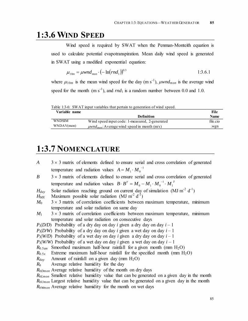
CHAPTER 1:3: EQUATIONS—WEATHER GENERATOR
85
85
1:3.6 WIND SPEED Wind speed is required by SWAT when the Penman-Monteith equation is
used to calculate potential evapotranspiration. Mean daily wind speed is generated
in SWAT using a modified exponential equation:
3.0110 ln rndwndmonm 1:3.6.1
where 10m is the mean wind speed for the day (m s-1), wndmon is the average wind
speed for the month (m s-1), and rnd1 is a random number between 0.0 and 1.0.
Table 1:3-6: SWAT input variables that pertain to generation of wind speed.
Variable name Definition
File Name
WNDSIM Wind speed input code: 1-measured, 2-generated file.cio WNDAV(mon) wndmon: Average wind speed in month (m/s) .wgn
1:3.7 NOMENCLATURE A 3 3 matrix of elements defined to ensure serial and cross correlation of generated
temperature and radiation values 101
MMA
B 3 3 matrix of elements defined to ensure serial and cross correlation of generated temperature and radiation values TT MMMMBB 1
1010
Hday Solar radiation reaching ground on current day of simulation (MJ m-2 d-1) HMX Maximum possible solar radiation (MJ m-2 d-1) M0 3 3 matrix of correlation coefficients between maximum temperature, minimum
temperature and solar radiation on same day M1 3 3 matrix of correlation coefficients between maximum temperature, minimum
temperature and solar radiation on consecutive days Pi(D/D) Probability of a dry day on day i given a dry day on day i – 1 Pi(D/W) Probability of a dry day on day i given a wet day on day i – 1 Pi(W/D) Probability of a wet day on day i given a dry day on day i – 1 Pi(W/W) Probability of a wet day on day i given a wet day on day i – 1 R0.5sm Smoothed maximum half-hour rainfall for a given month (mm H2O) R0.5x Extreme maximum half-hour rainfall for the specified month (mm H2O) Rday Amount of rainfall on a given day (mm H2O) Rh Average relative humidity for the day RhDmon Average relative humidity of the month on dry days RhLmon Smallest relative humidity value that can be generated on a given day in the month RhUmon Largest relative humidity value that can be generated on a given day in the month RhWmon Average relative humidity for the month on wet days
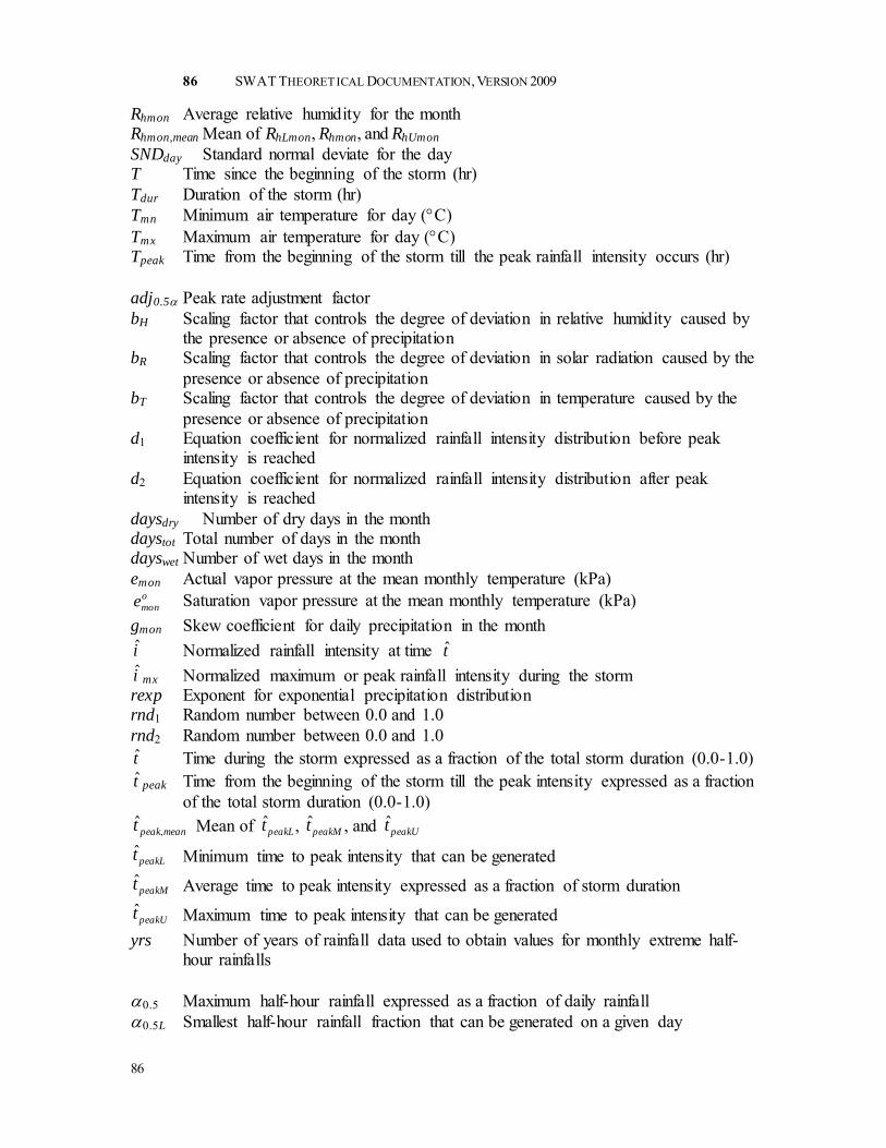
86 SWAT THEORETICAL DOCUMENTATION, VERSION 2009
86
Rhmon Average relative humidity for the month Rhmon,mean Mean of RhLmon, Rhmon, and RhUmon SNDday Standard normal deviate for the day T Time since the beginning of the storm (hr) Tdur Duration of the storm (hr) Tmn Minimum air temperature for day (C) Tmx Maximum air temperature for day (C) Tpeak Time from the beginning of the storm till the peak rainfall intensity occurs (hr) adj0.5 Peak rate adjustment factor bH Scaling factor that controls the degree of deviation in relative humidity caused by
the presence or absence of precipitation bR Scaling factor that controls the degree of deviation in solar radiation caused by the
presence or absence of precipitation bT Scaling factor that controls the degree of deviation in temperature caused by the
presence or absence of precipitation d1 Equation coefficient for normalized rainfall intensity distribution before peak
intensity is reached
d2 Equation coefficient for normalized rainfall intensity distribution after peak intensity is reached
daysdry Number of dry days in the month daystot Total number of days in the month dayswet Number of wet days in the month emon Actual vapor pressure at the mean monthly temperature (kPa)
o
mone Saturation vapor pressure at the mean monthly temperature (kPa) gmon Skew coefficient for daily precipitation in the month i Normalized rainfall intensity at time t
i mx Normalized maximum or peak rainfall intensity during the storm rexp Exponent for exponential precipitation distribution rnd1 Random number between 0.0 and 1.0 rnd2 Random number between 0.0 and 1.0 t Time during the storm expressed as a fraction of the total storm duration (0.0-1.0) t peak Time from the beginning of the storm till the peak intensity expressed as a fraction
of the total storm duration (0.0-1.0) meanpeakt ,
ˆ Mean of peakLt , peakMt , and peakUt
Minimum time to peak intensity that can be generated
Average time to peak intensity expressed as a fraction of storm duration
Maximum time to peak intensity that can be generated
yrs Number of years of rainfall data used to obtain values for monthly extreme half-hour rainfalls
0.5 Maximum half-hour rainfall expressed as a fraction of daily rainfall 0.5L Smallest half-hour rainfall fraction that can be generated on a given day
peakLt
peakMt
peakUt

CHAPTER 1:3: EQUATIONS—WEATHER GENERATOR
87
87
0.5mon Average maximum half-hour rainfall fraction for the month
0.5meanMean of 0.5L, 0.5mon, 0.5U 0.5U Largest half-hour rainfall fraction that can be generated on a given day
1 Equation coefficient for rainfall intensity before peak intensity is reached (hr) 2 Equation coefficient for rainfall intensity after peak intensity is reached (hr) i 3 1 matrix of independent random components mon Standard deviation of daily rainfall (mm H2O) for the month mnmonStandard deviation for daily minimum temperature during the month (C) mxmonStandard deviation for daily maximum temperature during the month (C) radmon Standard deviation for daily solar radiation during the month (MJ m-2) 0(j,k) Correlation coefficient between variables j and k on the same day where j and k
may be set to 1 (maximum temperature), 2 (minimum temperature) or 3 (solar radiation)
1(j,k) Correlation coefficient between variable j and k with variable k lagged one day with respect to variable j
mon Mean daily rainfall (mm H2O) for the month DmxmonAverage daily maximum temperature of the month on dry days (C) Dradmon Average daily solar radiation of the month on dry days (MJ m-2) WmxmonAverage daily maximum temperature of the month on wet days (C) Wradmon Average daily solar radiation of the month on wet days (MJ m-2) dewmon Average dew point temperature for the month (C) mnmonAverage daily minimum temperature for the month (C) mxmonAverage daily maximum temperature for the month (C) radmon Average daily solar radiation for the month (MJ m-2) tmpmon Mean air temperature for the month (C) wndmon Average wind speed for the month (m s-1) 10m Mean wind speed for the day at height of 10 meters (m s-1) i(j) 3 1 matrix for day i whose elements are residuals of maximum temperature (j =
1), minimum temperature (j = 2) and solar radiation (j = 3),
1:3.8 REFERENCES
Fiering, M.B. 1967. Streamflow synthesis. Harvard University Press, Cambridge.
Matalas, N.C. 1967. Mathematical assessment of synthetic hydrology. Water
Resources Res. 3(4):937-945.
Nicks, A.D. 1974. Stochastic generation of the occurrence, pattern, and location of
maximum amount of daily rainfall. p. 154-171. In Proc. Symp. Statistical
Hydrology, Aug.-Sept. 1971, Tuscon, AZ. U.S. Department of Agriculture,
Misc. Publ. No. 1275.

88 SWAT THEORETICAL DOCUMENTATION, VERSION 2009
88
Nicks, A.D., L.J. Lane, and G.A. Gander. 1995. Chapter 2: Weather generator. p.
2.1-2.22. In D.C. Flanagan and M.A. Nearing (ed.) USDA-Water Erosion
Prediction Project: Hillslope profile and watershed model documentation.
NSERL Report #10, National Soil Erosion Research Laboratory, West
Lafayette, IN.
Richardson, C.W. 1982. Dependence structure of daily temperature and solar
radiation. Trans. ASAE 25(3):735-739.
Richardson, C.W. 1981. Stochastic simulation of daily precipitation, temperature,
and solar radiation. Water Resources Res. 17(1):182-190.
Richardson, C.W. and D.A. Wright. 1984. WGEN: a model for generating daily
weather variables. U.S. Department of Agriculture, Agricultural Research
Service, ARS-8.
Sharpley, A.N. and J.R. Williams, eds. 1990. EPIC-Erosion Productivity Impact
Calculator, 1. model documentation. U.S. Department of Agriculture,
Agricultural Research Service, Tech. Bull. 1768.
Williams, J.R. 1995. Chapter 25. The EPIC Model. p. 909-1000. In Computer
Models of Watershed Hydrology. Water Resources Publications. Highlands
Ranch, CO.

CHAPTER 1:3: EQUATIONS—WEATHER GENERATOR
89
89

90
SECTION 1 CHAPTER 4
EQUATIONS:
CLIMATE CUSTOMIZATION
SWAT is capable of simulating a number of climate customization
options. Orographic impacts on temperature and precipitation for watersheds in
mountainous regions can be simulated. The model will also modify climate inputs
for simulations that are looking at the impact of climatic change in a given
watershed. Finally, SWAT allows a weather forecast period to be incorporated
into a simulation to study the effects of predicted weather in a watershed.
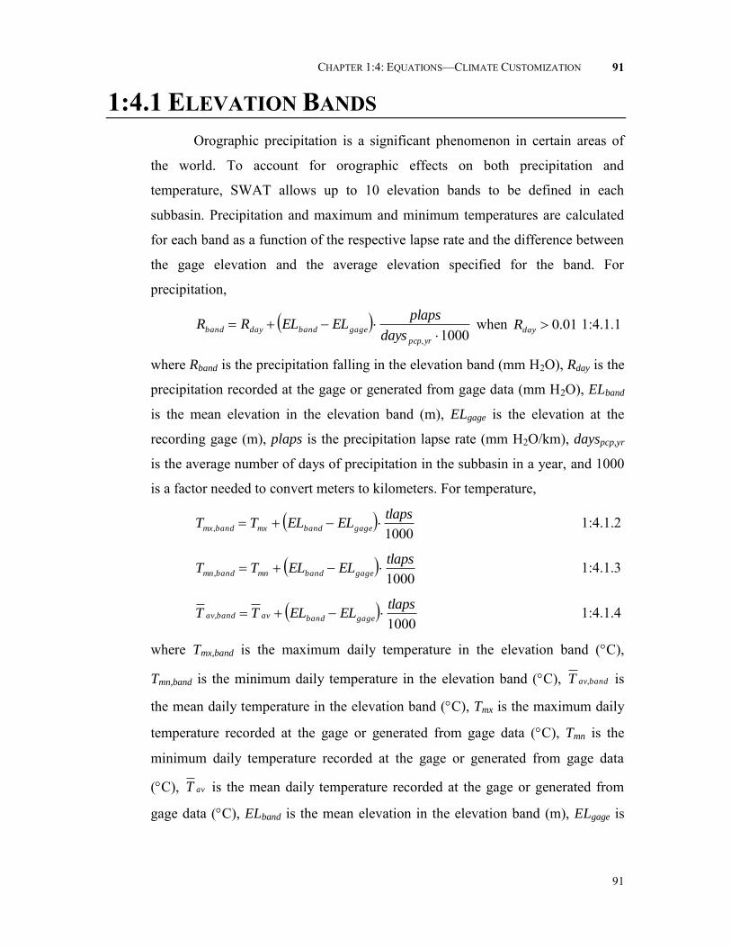
CHAPTER 1:4: EQUATIONS—CLIMATE CUSTOMIZATION
91
91
1:4.1 ELEVATION BANDS
Orographic precipitation is a significant phenomenon in certain areas of
the world. To account for orographic effects on both precipitation and
temperature, SWAT allows up to 10 elevation bands to be defined in each
subbasin. Precipitation and maximum and minimum temperatures are calculated
for each band as a function of the respective lapse rate and the difference between
the gage elevation and the average elevation specified for the band. For
precipitation,
1000,
yrpcp
gagebanddaybanddays
plapsELELRR when 01.0dayR 1:4.1.1
where Rband is the precipitation falling in the elevation band (mm H2O), Rday is the
precipitation recorded at the gage or generated from gage data (mm H2O), ELband
is the mean elevation in the elevation band (m), ELgage is the elevation at the
recording gage (m), plaps is the precipitation lapse rate (mm H2O/km), dayspcp,yr
is the average number of days of precipitation in the subbasin in a year, and 1000
is a factor needed to convert meters to kilometers. For temperature,
1000,tlaps
ELELTT gagebandmxbandmx 1:4.1.2
1000,tlaps
ELELTT gagebandmnbandmn 1:4.1.3
1000
,tlaps
ELELTT gagebandavbandav 1:4.1.4
where Tmx,band is the maximum daily temperature in the elevation band (C),
Tmn,band is the minimum daily temperature in the elevation band (C), bandavT , is
the mean daily temperature in the elevation band (C), Tmx is the maximum daily
temperature recorded at the gage or generated from gage data (C), Tmn is the
minimum daily temperature recorded at the gage or generated from gage data
(C), avT is the mean daily temperature recorded at the gage or generated from
gage data (C), ELband is the mean elevation in the elevation band (m), ELgage is

92 SWAT THEORETICAL DOCUMENTATION, VERSION 2009
92
the elevation at the recording gage (m), tlaps is the temperature lapse rate
(C/km), and 1000 is a factor needed to convert meters to kilometers.
Once the precipitation and temperature values have been calculated for
each elevation band in the subbasin, new average subbasin precipitation and
temperature values are calculated:
b
bnd
bndbandday frRR1
1:4.1.5
b
bnd
bndbandmxmx frTT1
, 1:4.1.6
b
bnd
bndbandmnmn frTT1
, 1:4.1.7
b
bnd
bndbandavav frTT1
, 1:4.1.8
where Rday is the daily average precipitation adjusted for orographic effects (mm
H2O), Tmx is the daily maximum temperature adjusted for orographic effects (C),
Tmn is the daily minimum temperature adjusted for orographic effects (C), avT is
the daily mean temperature adjusted for orographic effects (C), Rband is the
precipitation falling in elevation band bnd (mm H2O), Tmx,band is the maximum
daily temperature in elevation band bnd (C), Tmn,band is the minimum daily
temperature in elevation band bnd (C), bandavT , is the mean daily temperature in
elevation band bnd (C), frbnd is the fraction of subbasin area within the elevation
band, and b is the total number of elevation bands in the subbasin.
The only processes modeled separately for each individual elevation band
are the accumulation, sublimation and melting of snow. As with the initial
precipitation and temperature data, after amounts of sublimation and snow melt
are determined for each elevation band, subbasin average values are calculated.
These average values are the values that are used in the remainder of the
simulation and reported in the output files.

CHAPTER 1:4: EQUATIONS—CLIMATE CUSTOMIZATION
93
93
Table 1:4-1: SWAT input variables that pertain to orographic effects.
Variable Name
Definition Input File
ELEVB ELband: Elevation at center of the elevation band (m) .sub ELEVB_FR frbnd: Fraction of subbasin area within the elevation band. .sub WELEV ELgage: Elevation of recording gage whose data is used to calculate
values in .wgn file (m) .wgn
ELEVATION ELgage: Elevation of precipitation recording gage (m) .pcp ELEVATION ELgage: Elevation of temperature recording gage (m) .tmp PLAPS plaps: Precipitation lapse rate (mm H2O/km) .sub PCPD(mon) average number of days of precipitation in month
dayspcp,yr = (PCPD(mon) for a subbasin .wgn
TLAPS tlaps: Temperature lapse rate (C/km) .sub PRECIPITATION Rday: Daily precipitation (mm H2O) .pcp MAX TEMP Tmx: Daily maximum temperature (C) .tmp MIN TEMP Tmn: Daily minimum temperature (C) .tmp
1:4.2 CLIMATE CHANGE The impact of global climate change on water supply is a major area of
research. Climate change can be simulated with SWAT by manipulating the
climatic input that is read into the model (precipitation, temperature, solar
radiation, relative humidity, wind speed, potential evapotranspiration and weather
generator parameters). A less time-consuming method is to set adjustment factors
for the various climatic inputs.
SWAT will allow users to adjust precipitation, temperature, solar
radiation, relative humidity, and carbon dioxide levels in each subbasin. The
alteration of precipitation, temperature, solar radiation and relative humidity are
straightforward:
1001 pcp
dayday
adjRR 1:4.2.1
where Rday is the precipitation falling in the subbasin on a given day (mm H2O),
and adjpcp is the % change in rainfall.
tmpmxmx adjTT 1:4.2.2
where Tmx is the daily maximum temperature (C), and adjtmp is the change in
temperature (C).
tmpmnmn adjTT 1:4.2.3

94 SWAT THEORETICAL DOCUMENTATION, VERSION 2009
94
where Tmn is the daily minimum temperature (C), and adjtmp is the change in
temperature (C).
tmpavav adjTT 1:4.2.4
where avT is the daily mean temperature (C), and adjtmp is the change in
temperature (C).
raddayday adjHH 1:4.2.5
where Hday is the daily solar radiation reaching the earth’s surface (MJ m-2), and
adjrad is the change in radiation (MJ m-2 d-1).
hmdhh adjRR 1:4.2.6
where Rh is the relative humidity for the day expressed as a fraction, and adjhmd is
the change in relative humidity expressed as a fraction.
SWAT allows the adjustment terms to vary from month to month so that
the user is able to simulate seasonal changes in climatic conditions.
Changes in carbon dioxide levels impact plant growth. As carbon dioxide
levels increase, plant productivity increases and plant water requirements go
down. The equations used to account for the impact of carbon dioxide levels on
plant water requirements are reviewed in Chapters 2:2 and 5:2. When carbon
dioxide climate change effects are being simulated, the Penman-Monteith
equation must be used to calculate potential evapotranspiration. This method has
been modified to account for CO2 impacts on potential evapotranspiration levels.
Table 1:4-2: SWAT input variables that pertain to climate change.
Variable Name
Definition Input File
RFINC(mon) adjpcp: % change in rainfall for month .sub TMPINC(mon) adjtmp: increase or decrease in temperature for month (C) .sub RADINC(mon) adjrad: increase or decrease in solar radiation reaching earth’s
surface for month (MJ m-2) .sub
HUMINC(mon) adjhmd: increase or decrease in relative humidity for month .sub CO2 CO2: carbon dioxide level in subbasin (ppmv) .sub IPET Potential evapotranspiration method .bsn

CHAPTER 1:4: EQUATIONS—CLIMATE CUSTOMIZATION
95
95
1:4.3 WEATHER FORECAST INCORPORATION Being able to assess the impact of predicted weather in a watershed is
useful for some applications. For example, reservoir management can better time
needed water releases if they know the impact of storms in the near future.
SWAT allows a forecast period to be defined in a simulation. The
simulation is split into two parts. During the first portion of the simulation,
climatic data is read in from input files or generated using the long-term averages
input by the user in the weather generator (.wgn) file. When the simulation
reaches the first day of the forecast period (defined by FCSTDAY and FCSTYR
in file.cio) the model replaces the long-term weather generator averages with
averages provided for the forecast period. All climatic data required by SWAT is
generated during the forecast period.
Forecast data provided by the U.S. National Weather Service is
summarized by region. SWAT allows the user to incorporate data for multiple
regions within one simulation. The forecast region number assigned to a subbasin
must correspond to a forecast region number given for a specific dataset in the
forecast input file (.cst).
SWAT allows the user to define alternative temperature and precipitation
averages for the forecast period to generate daily precipitation and temperature
values. For temperature, the user specifies the average maximum and minimum
air temperature and the standard deviation for these averages. For precipitation,
the user specifies the average amount of precipitation falling by month along with
the standard deviation and skew coefficient for that average. The user must also
define the wet/dry day probabilities and the average number of days of
precipitation expected.
The forecast period must be simulated a number of times to obtain a
distribution of possible weather scenarios. The user defines the number of model
runs made (FCSTCYCLES in file.cio). A minimum of 20 cycles is recommended.
The only difference between forecast scenarios is the value of the random number
seeds used to generate daily weather values.

96 SWAT THEORETICAL DOCUMENTATION, VERSION 2009
96
Table 1:4-3: SWAT input variables that pertain to forecast incorporation.
Variable Name
Definition Input File
FCSTDAY First day of forecast period (julian date). file.cio FCSTYR Year that forecast period begins. file.cio FCSTCYCLES Number of times forecast period is simulated. file.cio FCSTFILE Name of input file containing forecast data. file.cio FCST_REG Forecast region number .sub, .cst FCST_REGTOT Total number of forecast regions used in watershed .cst FTMPMX(mon) mxmon: average maximum air temperature for month (C) .cst FTMPMN(mon) mnmon: average minimum air temperature for month (C) .cst FTMPSTDMX(mon) mxmon: standard deviation for maximum air temperature in
month (C) .cst
FTMPSTDMN(mon) mnmon: standard deviation for minimum air temperature in month (C)
.cst
FPCPMM(mon) average amount of precipitation falling in month (mm H2O) .cst FPCPSTD(mon) mon: standard deviation for daily precipitation in month (mm
H2O) .cst
FPCPSKW(mon) gmon: skew coefficient for daily precipitation in month .cst FPR_W(1,mon) Pi(W/D): probability of a wet day following a dry day in month .cst FPR_W(2,mon) Pi(W/W): probability of a wet day following a wet day in
month .cst
FPCPD(mon) average number of days of precipitation in month .cst
1:4.4 NOMENCLATURE CO2 Concentration of carbon dioxide in the atmosphere (ppmv) ELband Mean elevation in the elevation band (m) ELgage Elevation at the precipitation, temperature, or weather generator data recording
gage (m) Hday Solar radiation reaching ground on current day of simulation (MJ m-2 d-1) Rband Precipitation falling in the elevation band (mm H2O) Rday Amount of rainfall on a given day (mm H2O) Rh Average relative humidity for the day Tmn Minimum air temperature for day (C) Tmn,band Minimum daily temperature in the elevation band (C) Tmx Maximum air temperature for day (C) Tmx,band Maximum daily temperature in the elevation band (C)
avT Mean air temperature for day (C) bandavT , Mean daily temperature in the elevation band (C)
adjhmd Change in relative humidity expressed as a fraction
adjpcp % change in rainfall adjrad Change in radiation (MJ m-2 d-1) adjtmp Change in temperature (C) dayspcp,yr Average number of days of precipitation in the subbasin in a year frbnd Fraction of subbasin area within the elevation band plaps Precipitation lapse rate (mm H2O/km) tlaps Temperature lapse rate (C/km)

CHAPTER 1:4: EQUATIONS—CLIMATE CUSTOMIZATION
97
97

HYDROLOGY
The land phase of the hydrologic cycle is based
on the water balance equation:
where SWt is the final soil water content (mm H2O), SW0
is the initial soil water content (mm H2O), t is the time
(days), Rday is the amount of precipitation on day i (mm
H2O), Qsurf is the amount of surface runoff on day i (mm
H2O), Ea is the amount of evapotranspiration on day i
(mm H2O), wseep is the amount of percolation and bypass
flow exiting the soil profile bottom on day i (mm H2O),
and Qgw is the amount of return flow on day i (mm
H2O).

98
SECTION 2 CHAPTER 1
EQUATIONS:
SURFACE RUNOFF
Surface runoff occurs whenever the rate of water application to the ground
surface exceeds the rate of infiltration. When water is initially applied to a dry
soil, the infiltration rate is usually very high. However, it will decrease as the soil
becomes wetter. When the application rate is higher than the infiltration rate,
surface depressions begin to fill. If the application rate continues to be higher than
the infiltration rate once all surface depressions have filled, surface runoff will
commence.
SWAT provides two methods for estimating surface runoff: the SCS curve
number procedure (SCS, 1972) and the Green & Ampt infiltration method (1911).

CHAPTER 2:1: EQUATIONS—SURFACE RUNOFF
99
99
2:1.1 RUNOFF VOLUME: SCS CURVE NUMBER PROCEDURE
The SCS runoff equation is an empirical model that came into common use in the
1950s. It was the product of more than 20 years of studies involving rainfall-runoff
relationships from small rural watersheds across the U.S. The model was developed to
provide a consistent basis for estimating the amounts of runoff under varying land use
and soil types (Rallison and Miller, 1981).
The SCS curve number equation is (SCS, 1972):
SIR
IRQ
aday
aday
surf
2
2:1.1.1
where Qsurf is the accumulated runoff or rainfall excess (mm H2O), Rday is the rainfall
depth for the day (mm H2O), Ia is the initial abstractions which includes surface storage,
interception and infiltration prior to runoff (mm H2O), and S is the retention parameter
(mm H2O). The retention parameter varies spatially due to changes in soils, land use,
management and slope and temporally due to changes in soil water content. The retention
parameter is defined as:
1010004.25
CNS 2:1.1.2
where CN is the curve number for the day. The initial abstractions, Ia, is commonly
approximated as 0.2S and equation 2:1.1.1 becomes
SR
SRQ
day
day
surf 8.02.0 2
2:1.1.3
Runoff will only occur when Rday > Ia. A graphical solution of equation 2:1.1.3 for
different curve number values is presented in Figure 2:1-1.

100 SWAT THEORETICAL DOCUMENTATION, VERSION 2009
100
Figure 2:1-1: Relationship of runoff to rainfall in SCS curve number method.
2:1.1.1 SCS CURVE NUMBER The SCS curve number is a function of the soil’s permeability, land use and
antecedent soil water conditions. Typical curve numbers for moisture condition II
are listed in tables 2:1-1, 2:1-2 and 2:1-3 for various land covers and soil types
(SCS Engineering Division, 1986). These values are appropriate for a 5% slope. Table 2:1-1: Runoff curve numbers for cultivated agricultural lands (from SCS Engineering Division, 1986)
Cover Hydrologic Soil Group Land Use
Treatment or practice
Hydrologic condition
A
B
C
D
Fallow Bare soil - - - - 77 86 91 94 Crop residue cover Poor 76 85 90 93 Good 74 83 88 90 Row crops Straight row Poor 72 81 88 91 Good 67 78 85 89 Straight row w/ residue Poor 71 80 87 90 Good 64 75 82 85 Contoured Poor 70 79 84 88 Good 65 75 82 86 Contoured w/ residue Poor 69 78 83 87 Good 64 74 81 85 Contoured & terraced Poor 66 74 80 82 Good 62 71 78 81 Contoured & terraced w/ residue Poor 65 73 79 81 Good 61 70 77 80 Small grains Straight row Poor 65 76 84 88 Good 63 75 83 87 Straight row w/ residue Poor 64 75 83 86
Crop residue cover applies only if residue is on at least 5% of the surface throughout the year.

CHAPTER 2:1: EQUATIONS—SURFACE RUNOFF
101
101
Table 2:1-1, cont.: Runoff curve numbers for cultivated agricultural lands Cover
Hydrologic Soil Group Land Use
Treatment or practice
Hydrologic condition
A
B
C
D
Good 60 72 80 84 Contoured Poor 63 74 82 85 Good 61 73 81 84 Contoured w/ residue Poor 62 73 81 84 Good 60 72 80 83 Contoured & terraced Poor 61 72 79 82 Good 59 70 78 81 Contoured & terraced w/ residue Poor 60 71 78 81 Good 58 69 77 80 Close-seeded or broadcast legumes or rotation
Straight row Poor 66 77 85 89 Good 58 72 81 85 Contoured Poor 64 75 83 85 Good 55 69 78 83
Contoured & terraced Poor 63 73 80 83 Good 51 67 76 80
Table 2:1-2: Runoff curve numbers for other agricultural lands (from SCS Engineering Division, 1986)
Cover Hydrologic Soil Group Cover Type
Hydrologic condition
A
B
C
D
Pasture, grassland, or range—continuous forage for grazing1 Poor 68 79 86 89 Fair 49 69 79 84 Good 39 61 74 80 Meadow—continuous grass, protected from grazing and generally mowed for hay - - - - 30 58 71 78 Brush—brush-weed-grass mixture with brush the major element2 Poor 48 67 77 83 Fair 35 56 70 77 Good 30 48 65 73 Woods—grass combination (orchard or tree farm) Poor 57 73 82 86 Fair 43 65 76 82 Good 32 58 72 79 Woods3 Poor 45 66 77 83 Fair 36 60 73 79 Good 30 55 70 77 Farmsteads—buildings, lanes, driveways, and surrounding lots. - - - - 59 74 82 86
Table 2:1-3: Runoff curve numbers for urban areas§ (from SCS Engineering Division, 1986)
Cover Hydrologic Soil Group Cover Type
Hydrologic condition
Average % impervious area
A
B
C
D
Fully developed urban areas Open spaces (lawns, parks, golf courses, cemeteries, etc.)† Poor 68 79 86 89 Fair 49 69 79 84 Good 39 61 74 80 Impervious areas: Paved parking lots, roofs, driveways, etc. (excl. right-of-way) - - - - 98 98 98 98 Paved streets and roads; open ditches (incl. right-of-way) - - - - 83 89 92 93 Gravel streets and roads (including right-of-way) - - - - 76 85 89 91 Dirt streets and roads (including right-of way) - - - - 72 82 87 89
1 Poor: < 50% ground cover or heavily grazed with no mulch; Fair: 50 to 75% ground cover and not heavily grazed; Good: > 75% ground cover and lightly or only occasionally grazed 2 Poor: < 50% ground cover; Fair: 50 to 75% ground cover; Good: > 75% ground cover 3 Poor: Forest litter, small trees, and brush are destroyed by heavy grazing or regular burning; Fair: Woods are grazed but not burned, and some forest litter covers the soil; Good: Woods are protected from grazing, and lit ter and brush adequately cover the soil. § SWAT will automatically adjust curve numbers for impervious areas when IURBAN and URBLU are defined in the .hru file. Curve numbers from Table 6-3 should not be used in this instance. † Poor: grass cover < 50%; Fair: grass cover 50 to 75%; Good: grass cover > 75%

102 SWAT THEORETICAL DOCUMENTATION, VERSION 2009
102
Table 2:1-3, continued: Runoff curve number for urban areas Cover
Hydrologic Soil Group Cover Type
Hydrologic condition
Average % impervious area
A
B
C
D
Urban districts: Commercial and business 85% 89 92 94 95 Industrial 72% 81 88 91 93 Residential Districts by average lot size: 1/8 acre (0.05 ha) or less (town houses) 65% 77 85 90 92 1/4 acre (0.10 ha) 38% 61 75 83 87 1/3 acre (0.13 ha) 30% 57 72 81 86 1/2 acre (0.20 ha) 25% 54 70 80 85 1 acre (0.40 ha) 20% 51 68 79 84 2 acres (0.81 ha) 12% 46 65 77 82 Developing urban areas: Newly graded areas (pervious areas only, no vegetation) 77 86 91 94
2:1.1.1.1 SOIL HYDROLOGIC GROUPS The U.S. Natural Resource Conservation Service (NRCS)
classifies soils into four hydrologic groups based on infiltration
characteristics of the soils. NRCS Soil Survey Staff (1996) defines a
hydrologic group as a group of soils having similar runoff potential under
similar storm and cover conditions. Soil properties that influence runoff
potential are those that impact the minimum rate of infiltration for a bare
soil after prolonged wetting and when not frozen. These properties are
depth to seasonally high water table, saturated hydraulic conductivity, and
depth to a very slowly permeable layer. Soil may be placed in one of four
groups, A, B, C, and D, or three dual classes, A/D, B/D, and C/D.
Definitions of the classes are:
A: (Low runoff potential). The soils have a high infiltration rate even when thoroughly wetted. They chiefly consist of deep, well drained to excessively drained sands or gravels. They have a high rate of water transmission.
B: The soils have a moderate infiltration rate when thoroughly wetted. They chiefly are moderately deep to deep, moderately well-drained to well-drained soils that have moderately fine to moderately coarse textures. They have a moderate rate of water transmission.
C: The soils have a slow infiltration rate when thoroughly wetted. They chiefly have a layer that impedes downward movement of water or have moderately fine to fine texture. They have a slow rate of water transmission.

CHAPTER 2:1: EQUATIONS—SURFACE RUNOFF
103
103
D. (High runoff potential). The soils have a very slow infiltration rate when thoroughly wetted. They chiefly consist of clay soils that have a high swelling potential, soils that have a permanent water table, soils that have a claypan or clay layer at or near the surface, and shallow soils over nearly impervious material. They have a very slow rate of water transmission.
Dual hydrologic groups are given for certain wet soils that can be
adequately drained. The first letter applies to the drained condition, the
second to the undrained. Only soils that are rated D in their natural
condition are assigned to dual classes.
2:1.1.1.2 ANTECEDENT SOIL MOISTURE CONDITION SCS defines three antecedent moisture conditions: I—dry (wilting
point), II—average moisture, and III—wet (field capacity). The moisture
condition I curve number is the lowest value the daily curve number can
assume in dry conditions. The curve numbers for moisture conditions I
and III are calculated with the equations:
22
221 1000636.0533.2exp100
10020CNCN
CNCNCN
2:1.1.4
223 10000673.0exp CNCNCN 2:1.1.5
where CN1 is the moisture condition I curve number, CN2 is the moisture
condition II curve number, and CN3 is the moisture condition III curve
number.
2:1.1.1.3 RETENTION PARAMETER With SWAT2009, users are allowed to select between two
methods for calculating the retention parameter. The traditional method is
to allow the retention parameter to vary with soil profile water content. An
alternative added in SWAT2009 allows the retention parameter to vary
with accumulated plant evapotranspiration. Calculation of the daily CN
value as a function of plant evapotranspiration was added because the soil
moisture method was predicting too much runoff in shallow soils. By
calculating daily CN as a function of plant evapotranspiration, the value is
less dependent on soil storage and more dependent on antecedent climate.

104 SWAT THEORETICAL DOCUMENTATION, VERSION 2009
104
When the retention parameter varies with soil profile water
content, the following equation is used:
SWwwSW
SWSS
21max exp
1 2:1.1.6
where S is the retention parameter for a given day (mm), Smax is the
maximum value the retention parameter can achieve on any given day
(mm), SW is the soil water content of the entire profile excluding the
amount of water held in the profile at wilting point (mm H2O), and w1 and
w2 are shape coefficients. The maximum retention parameter value, Smax,
is calculated by solving equation 2:1.1.2 using CN1.
The shape coefficients are determined by solving equation 2:1.1.6
assuming that
1) the retention parameter for moisture condition I curve number
corresponds to wilting point soil profile water content,
2) the retention parameter for moisture condition III curve number
corresponds to field capacity soil profile water content, and
3) the soil has a curve number of 99 (S = 2.54) when completely
saturated.
FCwFCSS
FCw
21max3
1 1ln 2:1.1.7
FCSAT
SATS
SATFC
SS
FC
w
1max
1max3
2
54.21ln
1ln
2:1.1.8
where w1 is the first shape coefficient, w2 is the second shape coefficient,
FC is the amount of water in the soil profile at field capacity (mm H2O),
S3 is the retention parameter for the moisture condition III curve number,
Smax is the retention parameter for the moisture condition I curve number,
SAT is the amount of water in the soil profile when completely saturated
(mm H2O), and 2.54 is the retention parameter value for a curve number
of 99.

CHAPTER 2:1: EQUATIONS—SURFACE RUNOFF
105
105
When the retention parameter varies with plant evapotranspiration,
the following equation is used to update the retention parameter at the end
of every day:
surfday
prev
oprev QRS
ScncoefESS
max
*exp 2:1.1.9
where S is the retention parameter for a given day (mm), Sprev is the
retention parameter for the previous day (mm), Eo is the potential
evapotranspiration for the day (mm d-1), cncoef is the weighting
coefficient used to calculate the retention coefficient for daily curve
number calculations dependent on plant evapotranspiration, Smax is the
maximum value the retention parameter can achieve on any given day
(mm), Rday is the rainfall depth for the day (mm H2O), and Qsurf is the
surface runoff (mm H2O). The initial value of the retention parameter is
defined as max9.0 SS .
When the top layer of the soil is frozen, the retention parameter is
modified using the following equation:
SSS frz 000862.0exp1max 2:1.1.10
where Sfrz is the retention parameter adjusted for frozen conditions (mm),
Smax is the maximum value the retention parameter can achieve on any
given day (mm), and S is the retention parameter for a given moisture
content calculated with equation 2:1.1.6 (mm).
The daily curve number value adjusted for moisture content is
calculated by rearranging equation 2:1.1.2 and inserting the retention
parameter calculated for that moisture content:
254
25400
S
CN 2:1.1.11
where CN is the curve number on a given day and S is the retention
parameter calculated for the moisture content of the soil on that day.
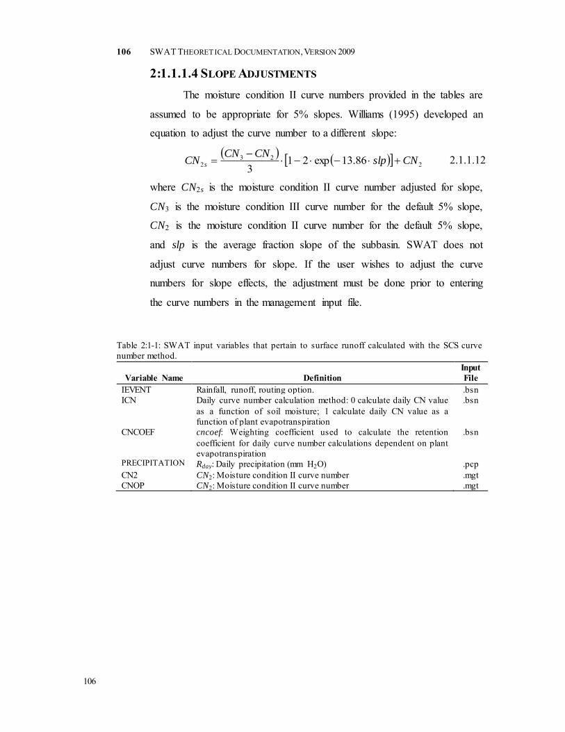
106 SWAT THEORETICAL DOCUMENTATION, VERSION 2009
106
2:1.1.1.4 SLOPE ADJUSTMENTS The moisture condition II curve numbers provided in the tables are
assumed to be appropriate for 5% slopes. Williams (1995) developed an
equation to adjust the curve number to a different slope:
2
232 86.13exp21
3CNslp
CNCNCN s
2.1.1.12
where CN2s is the moisture condition II curve number adjusted for slope,
CN3 is the moisture condition III curve number for the default 5% slope,
CN2 is the moisture condition II curve number for the default 5% slope,
and slp is the average fraction slope of the subbasin. SWAT does not
adjust curve numbers for slope. If the user wishes to adjust the curve
numbers for slope effects, the adjustment must be done prior to entering
the curve numbers in the management input file.
Table 2:1-1: SWAT input variables that pertain to surface runoff calculated with the SCS curve number method.
Variable Name
Definition
Input File
IEVENT Rainfall, runoff, routing option. .bsn ICN Daily curve number calculation method: 0 calculate daily CN value
as a function of soil moisture; 1 calculate daily CN value as a function of plant evapotranspiration
.bsn
CNCOEF cncoef: Weighting coefficient used to calculate the retention coefficient for daily curve number calculations dependent on plant evapotranspiration
.bsn
PRECIPITATION Rday: Daily precipitation (mm H2O) .pcp CN2 CN2: Moisture condition II curve number .mgt CNOP CN2: Moisture condition II curve number .mgt

CHAPTER 2:1: EQUATIONS—SURFACE RUNOFF
107
107
2:1.2 RUNOFF VOLUME: GREEN & AMPT INFILTRATION METHOD
The Green & Ampt equation was developed to predict infiltration
assuming excess water at the surface at all times (Green & Ampt, 1911). The
equation assumes that the soil profile is homogenous and antecedent moisture is
uniformly distributed in the profile. As water infiltrates into the soil, the model
assumes the soil above the wetting front is completely saturated and there is a
sharp break in moisture content at the wetting front. Figure 2:1-2 graphically
illustrates the difference between the moisture distribution with depth modeled by
the Green & Ampt equation and what occurs in reality.
Figure 2:1-2: Comparison of moisture content distribution modeled by Green & Ampt and a typical observed distribution.
Mein and Larson (1973) developed a methodology for determining
ponding time with infiltration using the Green & Ampt equation. The Green-
Ampt Mein-Larson excess rainfall method was incorporated into SWAT to
provide an alternative option for determining surface runoff. This method requires
sub-daily precipitation data supplied by the user.
The Green-Ampt Mein-Larson infiltration rate is defined as:
tinf
vwf
etinfF
Kf,
, 1
2:1.2.1

108 SWAT THEORETICAL DOCUMENTATION, VERSION 2009
108
where finf is the infiltration rate at time t (mm/hr), Ke is the effective hydraulic
conductivity (mm/hr), wf is the wetting front matric potential (mm), v is the
change in volumetric moisture content across the wetting front (mm/mm) and Finf
is the cumulative infiltration at time t (mm H2O).
When the rainfall intensity is less than the infiltration rate, all the rainfall
will infiltrate during the time period and the cumulative infiltration for that time
period is calculated:
ttinftinf RFF 1,, 2:1.2.2
where Finf,t is the cumulative infiltration for a given time step (mm H2O), Finf,t-1 is
the cumulative infiltration for the previous time step (mm H2O), and Rt is the
amount of rain falling during the time step (mm H2O).
The infiltration rate defined by equation 2:1.2.1 is a function of the
infiltrated volume, which in turn is a function of the infiltration rates in previous
time steps. To avoid numerical errors over long time steps, finf is replaced by
dtdFinf in equation 2:1.2.1 and integrated to obtain
vwftinf
vwftinf
vwfetinftinfF
FtKFF
1,
,1,, ln 2:1.2.3
Equation 2:1.2.3 must be solved iteratively for Finf,t, the cumulative infiltration at
the end of the time step. A successive substitution technique is used.
The Green-Ampt effective hydraulic conductivity parameter, Ke, is
approximately equivalent to one-half the saturated hydraulic conductivity of the
soil, Ksat (Bouwer, 1969). Nearing et al. (1996) developed an equation to calculate
the effective hydraulic conductivity as a function of saturated hydraulic
conductivity and curve number. This equation incorporates land cover impacts
into the calculated effective hydraulic conductivity. The equation for effective
hydraulic conductivity is:
2062.0exp051.01
82.56 286.0
CN
KK sat
e 2:1.2.4
where Ke is the effective hydraulic conductivity (mm/hr), Ksat is the saturated
hydraulic conductivity (mm/hr), and CN is the curve number.
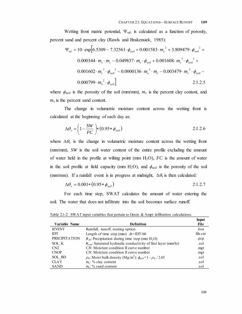
CHAPTER 2:1: EQUATIONS—SURFACE RUNOFF
109
109
Wetting front matric potential, wf, is calculated as a function of porosity,
percent sand and percent clay (Rawls and Brakensiek, 1985):
22 809479.3001583.032561.75309.6exp10 soilcsoilwf m
22001608.0049837.0000344.0 soilssoilscs mmmm
soilccssoilc mmmm 2222 003479.00000136.0001602.0
soilsm 2000799.0 2:1.2.5
where soil is the porosity of the soil (mm/mm), mc is the percent clay content, and
ms is the percent sand content.
The change in volumetric moisture content across the wetting front is
calculated at the beginning of each day as:
soilvFC
SW
95.01 2:1.2.6
where v is the change in volumetric moisture content across the wetting front
(mm/mm), SW is the soil water content of the entire profile excluding the amount
of water held in the profile at wilting point (mm H2O), FC is the amount of water
in the soil profile at field capacity (mm H2O), and soil is the porosity of the soil
(mm/mm). If a rainfall event is in progress at midnight, v is then calculated:
soilv 95.0001.0 2:1.2.7
For each time step, SWAT calculates the amount of water entering the
soil. The water that does not infiltrate into the soil becomes surface runoff.
Table 2:1-2: SWAT input variables that pertain to Green & Ampt infiltration calculations.
Variable Name
Definition Input File
IEVENT Rainfall, runoff, routing option. .bsn IDT Length of time step (min): t=IDT/60 file.cio PRECIPITATION Rt: Precipitation during time step (mm H2O) .pcp SOL_K Ksat: Saturated hydraulic conductivity of first layer (mm/hr) .sol CN2 CN: Moisture condition II curve number .mgt CNOP CN: Moisture condition II curve number .mgt SOL_BD b: Moist bulk density (Mg/m3): soil=1 - b / 2.65 .sol CLAY mc: % clay content .sol SAND ms: % sand content .sol

110 SWAT THEORETICAL DOCUMENTATION, VERSION 2009
110
2:1.3 PEAK RUNOFF RATE The peak runoff rate is the maximum runoff flow rate that occurs with a
given rainfall event. The peak runoff rate is an indicator of the erosive power of a
storm and is used to predict sediment loss. SWAT calculates the peak runoff rate
with a modified rational method.
The rational method is widely used in the design of ditches, channels and
storm water control systems. The rational method is based on the assumption that
if a rainfall of intensity i begins at time t = 0 and continues indefinitely, the rate of
runoff will increase until the time of concentration, t = tconc, when the entire
subbasin area is contributing to flow at the outlet. The rational formula is:
6.3AreaiC
qpeak
2:1.3.1
where qpeak is the peak runoff rate (m3 s-1), C is the runoff coefficient, i is the
rainfall intensity (mm/hr), Area is the subbasin area (km2) and 3.6 is a unit
conversion factor.
2:1.3.1 TIME OF CONCENTRATION The time of concentration is the amount of time from the beginning of a
rainfall event until the entire subbasin area is contributing to flow at the outlet. In
other words, the time of concentration is the time for a drop of water to flow from
the remotest point in the subbasin to the subbasin outlet. The time of
concentration is calculated by summing the overland flow time (the time it takes
for flow from the remotest point in the subbasin to reach the channel) and the
channel flow time (the time it takes for flow in the upstream channels to reach the
outlet):
chovconc ttt 2:1.3.2
The equations in section 2:1.3 use the subbasin area rather than the HRU area. Unlike HRUs, subbasins are geographically contiguous areas. Using the subbasin area makes the equations for time of concentration and peak runoff rate easier to conceptualize. In the model, these calculations are performed at the HRU level. Two modifications are made to adapt the equations to HRUs. First, the area of the subbasin is replaced by the area of the HRU. Second, the channel length term, L, used in the channel flow time of concentration calculation is multiplied by the fraction of the subbasin area with the HRU of interest.

CHAPTER 2:1: EQUATIONS—SURFACE RUNOFF
111
111
where tconc is the time of concentration for a subbasin (hr), tov is the time of concentration for overland flow (hr), and tch is the time of concentration for channel flow (hr).
2:1.3.1.1 OVERLAND FLOW TIME OF CONCENTRATION The overland flow time of concentration, tov, can be computed
using the equation
ov
slp
ovv
Lt
3600 2:1.3.3
where Lslp is the subbasin slope length (m), vov is the overland flow velocity (m s-1) and 3600 is a unit conversion factor. The overland flow velocity can be estimated from Manning’s equation by considering a strip 1 meter wide down the sloping surface:
6.0
3.04.0
n
slpqv ov
ov
2:1.3.4
where qov is the average overland flow rate (m3 s-1), slp is the average slope in the subbasin (m m-1), and n is Manning’s roughness coefficient for the subbasin. Assuming an average flow rate of 6.35 mm/hr and converting units
6.0
3.04.0005.0n
slpLv
slp
ov
2:1.3.5
Substituting equation 2:1.3.5 into equation 2:1.3.3 gives
3.0
6.06.0
18 slp
nLt
slp
ov
2.1.3.6
Table 6-3: Values of Manning’s roughness coefficient, n, for overland flow (Engman, 1983). Characteristics of Land Surface Median Range Fallow, no residue 0.010 0.008-0.012 Conventional tillage, no residue 0.090 0.060-0.120 Conventional tillage, residue 0.190 0.160-0.220 Chisel plow, no residue 0.090 0.060-0.120 Chisel plow, residue 0.130 0.100-0.160 Fall disking, residue 0.400 0.300-0.500 No till, no residue 0.070 0.040-0.100 No till, 0.5-1 t/ha residue 0.120 0.070-0.170 No till, 2-9 t/ha residue 0.300 0.170-0.470 Rangeland, 20% cover 0.600 Short grass prairie 0.150 0.100-0.200 Dense grass 0.240 0.170-0.300 Bermudagrass 0.410 0.300-0.480

112 SWAT THEORETICAL DOCUMENTATION, VERSION 2009
112
2:1.3.1.2 CHANNEL FLOW TIME OF CONCENTRATION The channel flow time of concentration, tch, can be computed using
the equation:
c
cch
v
Lt
6.3 2:1.3.7
where Lc is the average flow channel length for the subbasin (km), vc is the
average channel velocity (m s-1), and 3.6 is a unit conversion factor.
The average channel flow length can be estimated using the
equation
cenc LLL 2:1.3.8
where L is the channel length from the most distant point to the subbasin
outlet (km), and Lcen is the distance along the channel to the subbasin
centroid (km). Assuming LLcen 5.0 , the average channel flow length is
LLc 71.0 2:1.3.9
The average velocity can be estimated from Manning’s equation
assuming a trapezoidal channel with 2:1 side slopes and a 10:1 bottom
width-depth ratio.
75.0
375.025.0489.0n
slpqv chch
c
2:1.3.10
where vc is the average channel velocity (m s-1), qch is the average channel
flow rate (m3 s-1), slpch is the channel slope (m m-1), and n is Manning’s
roughness coefficient for the channel. To express the average channel flow
rate in units of mm/hr, the following expression is used
6.3
* Areaqq ch
ch
2:1.3.11
where *chq is the average channel flow rate (mm hr-1), Area is the subbasin
area (km2), and 3.6 is a unit conversion factor. The average channel flow
rate is related to the unit source area flow rate (unit source area = 1 ha)
5.0*0
* 100 Areaqqch 2:1.3.12
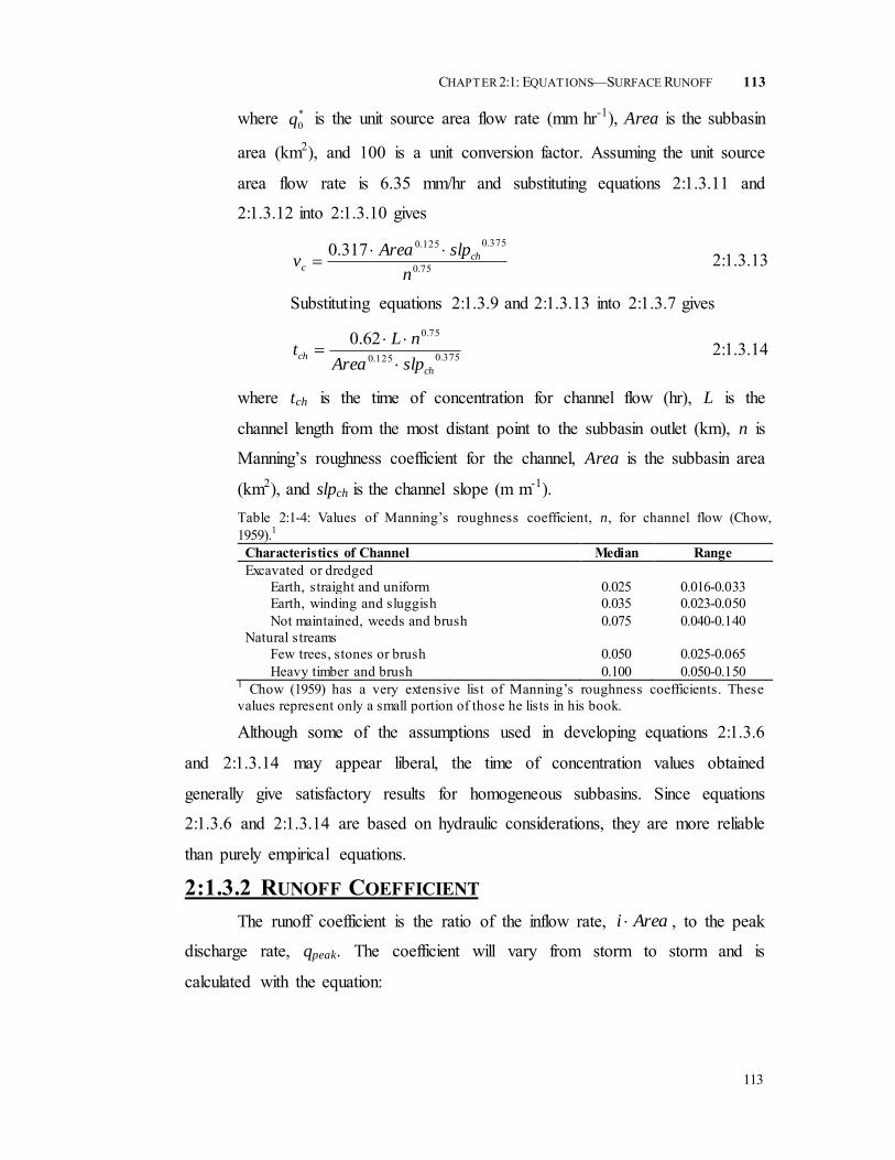
CHAPTER 2:1: EQUATIONS—SURFACE RUNOFF
113
113
where *0q is the unit source area flow rate (mm hr-1), Area is the subbasin
area (km2), and 100 is a unit conversion factor. Assuming the unit source
area flow rate is 6.35 mm/hr and substituting equations 2:1.3.11 and
2:1.3.12 into 2:1.3.10 gives
75.0
375.0125.0317.0n
slpAreav ch
c
2:1.3.13
Substituting equations 2:1.3.9 and 2:1.3.13 into 2:1.3.7 gives
375.0125.0
75.062.0
ch
chslpArea
nLt
2:1.3.14
where tch is the time of concentration for channel flow (hr), L is the
channel length from the most distant point to the subbasin outlet (km), n is
Manning’s roughness coefficient for the channel, Area is the subbasin area
(km2), and slpch is the channel slope (m m-1). Table 2:1-4: Values of Manning’s roughness coefficient, n, for channel flow (Chow, 1959).1
Characteristics of Channel Median Range Excavated or dredged
Earth, straight and uniform 0.025 0.016-0.033 Earth, winding and sluggish 0.035 0.023-0.050 Not maintained, weeds and brush 0.075 0.040-0.140
Natural streams Few trees, stones or brush 0.050 0.025-0.065 Heavy timber and brush 0.100 0.050-0.150
1 Chow (1959) has a very extensive list of Manning’s roughness coefficients. These values represent only a small portion of those he lists in his book.
Although some of the assumptions used in developing equations 2:1.3.6
and 2:1.3.14 may appear liberal, the time of concentration values obtained
generally give satisfactory results for homogeneous subbasins. Since equations
2:1.3.6 and 2:1.3.14 are based on hydraulic considerations, they are more reliable
than purely empirical equations.
2:1.3.2 RUNOFF COEFFICIENT The runoff coefficient is the ratio of the inflow rate, Areai , to the peak
discharge rate, qpeak. The coefficient will vary from storm to storm and is
calculated with the equation:

114 SWAT THEORETICAL DOCUMENTATION, VERSION 2009
114
day
surf
R
QC 2:1.3.15
where Qsurf is the surface runoff (mm H2O) and Rday is the rainfall for the day (mm
H2O).
2:1.3.3 RAINFALL INTENSITY The rainfall intensity is the average rainfall rate during the time of
concentration. Based on this definition, it can be calculated with the equation:
conc
tc
t
Ri 2.1.3.16
where i is the rainfall intensity (mm/hr), Rtc is the amount of rain falling during
the time of concentration (mm H2O), and tconc is the time of concentration for the
subbasin (hr).
An analysis of rainfall data collected by Hershfield (1961) for different
durations and frequencies showed that the amount of rain falling during the time
of concentration was proportional to the amount of rain falling during the 24-hr
period.
daytctc RR 2:1.3.17
where Rtc is the amount of rain falling during the time of concentration (mm
H2O), tc is the fraction of daily rainfall that occurs during the time of
concentration, and Rday is the amount of rain falling during the day (mm H2O).
For short duration storms, all or most of the rain will fall during the time
of concentration, causing tc to approach its upper limit of 1.0. The minimum
value of tc would be seen in storms of uniform intensity (i24 = i). This minimum
value can be defined by substituting the products of time and rainfall intensity
into equation 2:1.3.17
242424
min,concconc
day
tctc
t
i
ti
R
R
2:1.3.18
Thus, tc falls in the range tconc/24 tc 1.0.

CHAPTER 2:1: EQUATIONS—SURFACE RUNOFF
115
115
SWAT estimates the fraction of rain falling in the time of concentration as
a function of the fraction of daily rain falling in the half-hour of highest intensity
rainfall.
5.01ln2exp1 conctc t 2:1.3.19
where 0.5 is the fraction of daily rain falling in the half-hour highest intensity
rainfall, and tconc is the time of concentration for the subbasin (hr). The
determination of a value for 0.5 is discussed in Chapters 1:2 and 1:3.
2:1.3.4 MODIFIED RATIONAL FORMULA The modified rational formula used to estimate peak flow rate is obtained
by substituting equations 2:1.3.15, 2:1.3.16, and 2:1.3.17 into equation 2:1.3.1
conc
surftc
peakt
AreaQq
6.3
2:1.3.20
where qpeak is the peak runoff rate (m3 s-1), tc is the fraction of daily rainfall that
occurs during the time of concentration, Qsurf is the surface runoff (mm H2O),
Area is the subbasin area (km2), tconc is the time of concentration for the subbasin
(hr) and 3.6 is a unit conversion factor.
Table 2:1-5: SWAT input variables that pertain to peak rate calculations.
Variable Name
Definition Input File
SUB_KM Area of the subbasin (km2) .sub HRU_FR Fraction of subbasin area contained in HRU .hru SLSUBBSN Lslp: Average slope length (m) .hru HRU_SLP slp: Average slope steepness (m/m) .hru OV_N n: Manning’s ―n‖ value for overland flow .hru CH_L(1) L: Longest tributary channel length in subbasin (km) .sub CH_S(1) slpch: Average slope of tributary channels (m/m) .sub CH_N(1) n: Manning’s ―n‖ value for tributary channels .sub
2:1.4 SURFACE RUNOFF LAG In large subbasins with a time of concentration greater than 1 day, only a
portion of the surface runoff will reach the main channel on the day it is
generated. SWAT incorporates a surface runoff storage feature to lag a portion of
the surface runoff release to the main channel.

116 SWAT THEORETICAL DOCUMENTATION, VERSION 2009
116
Once surface runoff is calculated with the curve number or Green & Ampt
method, the amount of surface runoff released to the main channel is calculated:
conc
istorsurfsurft
surlagQQQ exp11, 2:1.4.1
where Qsurf is the amount of surface runoff discharged to the main channel on a
given day (mm H2O), surfQ is the amount of surface runoff generated in the
subbasin on a given day (mm H2O), Qstor,i-1 is the surface runoff stored or lagged
from the previous day (mm H2O), surlag is the surface runoff lag coefficient, and
tconc is the time of concentration for the subbasin (hrs).
The expression
conct
surlagexp1 in equation 2:1.4.1 represents the
fraction of the total available water that will be allowed to enter the reach on any
one day. Figure 2:1-3 plots values for this expression at different values for surlag
and tconc.
Figure 2:1-3: Influence of surlag and tconc on fraction of surface runoff released.
Note that for a given time of concentration, as surlag decreases in value
more water is held in storage. The delay in release of surface runoff will smooth
the streamflow hydrograph simulated in the reach.
Table 2:1-6: SWAT input variables that pertain to surface runoff lag calculations.
Variable Name
Definition Input File
SURLAG surlag: surface runoff lag coefficient .bsn

CHAPTER 2:1: EQUATIONS—SURFACE RUNOFF
117
117
2:1.5 TRANSMISSION LOSSES Many semiarid and arid watersheds have ephemeral channels that abstract
large quantities of streamflow (Lane, 1982). The abstractions, or transmission
losses, reduce runoff volume as the flood wave travels downstream. Chapter 19 of
the SCS Hydrology Handbook (Lane, 1983) describes a procedure for estimating
transmission losses for ephemeral streams which has been incorporated into
SWAT. This method was developed to estimate transmission losses in the absence
of observed inflow-outflow data and assumes no lateral inflow or out-of-bank
flow contributions to runoff.
The prediction equation for runoff volume after transmission losses is
thriQsurfiQsurfxx
thriQsurf
fQsurf volvolvolba
volvolvol
,,
,,
0 2:1.5.1
where volQsurf,f is the volume of runoff after transmission losses (m3), ax is the
regression intercept for a channel of length L and width W (m3), bx is the
regression slope for a channel of length L and width W, volQsurf,i is the volume of
runoff prior to transmission losses (m3), and volthr is the threshold volume for a
channel of length L and width W (m3). The threshold volume is
x
xthr
b
avol 2:1.5.2
The corresponding equation for peak runoff rate is
ipeakxiQsurfxx
flw
fpeak qbvolbadur
q ,,, 13600
1
2:1.5.3
where qpeak,f is the peak rate after transmission losses (m3/s), durflw is the duration
of flow (hr), ax is the regression intercept for a channel of length L and width W
(m3), bx is the regression slope for a channel of length L and width W, volQsurf,i is
the volume of runoff prior to transmission losses (m3), qpeak,i is the peak rate
before accounting for transmission losses (m3/s). The duration of flow is
calculated with the equation:

118 SWAT THEORETICAL DOCUMENTATION, VERSION 2009
118
peak
surf
flwq
AreaQdur
6.3 2:1.5.4
where durflw is the duration of runoff flow (hr), Qsurf is the surface runoff (mm
H2O), Area is the area of the subbasin (km2), qpeak is the peak runoff rate (m3/s),
and 3.6 is a conversion factor.
In order to calculate the regression parameters for channels of differing
lengths and widths, the parameters of a unit channel are needed. A unit channel is
defined as a channel of length L = 1 km and width W = 1 m. The unit channel
parameters are calculated with the equations:
iQsurf
flwch
rvol
durKk
,
6466.21ln22.2 2:1.5.5
flwchr durKa 2258.0 2:1.5.6
rr kb 4905.0exp 2:1.5.7
where kr is the decay factor (m-1 km-1), ar is the unit channel regression intercept
(m3), br is the unit channel regression slope, Kch is the effective hydraulic
conductivity of the channel alluvium (mm/hr), durflw is the duration of runoff flow
(hr), and volQsurf,i is the initial volume of runoff (m3). The regression parameters
are
WLkb rx exp 2:1.5.8
x
r
rx b
b
aa
1
1 2:1.5.9
where ax is the regression intercept for a channel of length L and width W (m3), bx
is the regression slope for a channel of length L and width W, kr is the decay
factor (m-1 km-1), L is the channel length from the most distant point to the
subbasin outlet (km), W is the average width of flow, i.e. channel width (m) ar is
the unit channel regression intercept (m3), and br is the unit channel regression
slope.
Transmission losses from surface runoff are assumed to percolate into the
shallow aquifer.

CHAPTER 2:1: EQUATIONS—SURFACE RUNOFF
119
119
Table 2:1-7: SWAT input variables that pertain to transmission loss calculations.
Variable Name
Definition Input File
SUB_KM Area of the subbasin (km2) .sub HRU_FR Fraction of total subbasin area contained in HRU .hru CH_K(1) Kch: effective hydraulic conductivity (mm/hr) .sub CH_W(1) W: average width of tributary channel (m) .sub CH_L(1) L: Longest tributary channel length in subbasin (km) .sub
2:1.6 NOMENCLATURE Area Subbasin area (km2) C Runoff coefficient in peak runoff rate calculation CN Curve number CN1 Moisture condition I curve number CN2 Moisture condition II curve number CN2s Moisture condition II curve number adjusted for slope
CN3 Moisture condition III curve number Eo Potential evapotranspiration (mm d-1) Finf Cumulative infiltration at time t (mm H2O) FC Water content of soil profile at field capacity (mm H2O) Ia Initial abstractions which includes surface storage, interception and infiltration
prior to runoff (mm H2O) Kch Effective hydraulic conductivity of the channel alluvium (mm/hr) Ke Effective hydraulic conductivity (mm/hr) Ksat Saturated hydraulic conductivity (mm/hr) L Channel length from the most distant point to the subbasin outlet (km) Lc Average flow channel length for the subbasin (km) Lcen Distance along the channel to the subbasin centroid (km) Lslp Subbasin slope length (m) Qstor Surface runoff stored or lagged (mm H2O) Qsurf Accumulated runoff or rainfall excess (mm H2O) Rt Amount of rain falling during the time step (mm H2O) Rday Amount of rainfall on a given day (mm H2O) Rtc Amount of rain falling during the time of concentration (mm H2O) S Retention parameter in SCS curve number equation (mm) S3 Retention parameter for the moisture condition III curve number Sfrz Retention parameter adjusted for frozen conditions (mm) Smax Maximum value the retention parameter can achieve on any given day (mm) Sprev Retention parameter in SCS curve number equation from previous day (mm) SAT Amount of water in the soil profile when completely saturated (mm H2O), SW Amount of water in soil profile (mm H2O) W Average width of flow, i.e. channel width (m)
ar Unit channel regression intercept (m3)

120 SWAT THEORETICAL DOCUMENTATION, VERSION 2009
120
ax Regression intercept for a channel of length L and width W (m3) br Unit channel regression slope
bx Regression slope for a channel of length L and width W cncoef Weighting coefficient used to calculate the retention coefficient for daily curve
number calculations dependent on plant evapotranspiration durflw Duration of flow (hr) finf Infiltration rate (mm/hr) i Rainfall intensity (mm/hr) kr Decay factor (m-1 km-1) mc Percent clay content ms Percent sand content n Manning’s roughness coefficient for the subbasin or channel
*0q Unit source area flow rate (mm hr-1)
qch Average channel flow rate (m3 s-1) *chq Average channel flow rate (mm hr-1)
qov Average overland flow rate (m3 s-1) qpeak Peak runoff rate (m3/s) qpeak,f Peak rate after transmission losses (m3/s) qpeak,i Peak rate before accounting for transmission losses (m3/s) slp Average slope of the subbasin (% or m/m) slpch Average channel slope (m m-1) surlag Surface runoff lag coefficient tch Time of concentration for channel flow (hr) tconc Time of concentration for a subbasin (hr) tov Time of concentration for overland flow (hr) vc Average channel velocity (m s-1) vov Overland flow velocity (m s-1) volQsurf,f Volume of runoff after transmission losses (m3) volQsurf,i Volume of runoff prior to transmission losses (m3) volthr Threshold volume for a channel of length L and width W (m3) w1 Shape coefficient in retention parameter adjustments for soil moisture content w2 Shape coefficient in retention parameter adjustments for soil moisture content 0.5 Fraction of daily rain falling in the half-hour highest intensity rainfall, tc Fraction of daily rainfall that occurs during the time of concentration
soil Porosity of the soil (mm/mm) wf Wetting front matric potential (mm) v Volumetric moisture content (mm/mm)
2:1.7 REFERENCES Bouwer, H. 1969. Infiltration of water into nonuniform soil. Journal Irrigation and
Drainage Div., ASCE 95(IR4):451-462.

CHAPTER 2:1: EQUATIONS—SURFACE RUNOFF
121
121
Chow, V.T. 1959. Open-channel hydraulics. McGraw-Hill, New York. Engman, E.T. 1983. Roughness coefficients for routing surface runoff. Proc.
Spec. Conf. Frontiers of Hydraulic Engineering. Green, W.H. and G.A. Ampt. 1911. Studies on soil physics, 1. The flow of air and
water through soils. Journal of Agricultural Sciences 4:11-24. Hershfield, D.M. 1961. Rainfall frequency atlas of the United States for durations
from 30 minutes to 24 hours and return periods from 1 to 100 years. U.S. Dept. Commerce Tech. Paper No. 40.
Lane, L.J. 1983. Chapter 19: Transmission Losses. p.19-1–19-21. In Soil Conservation Service. National engineering handbook, section 4: hydrology. U.S. Government Printing Office, Washington, D.C.
Lane, L.J. 1982. Distributed model for small semi-arid watersheds. J. Hydraulic Eng., ASCE, 108(HY10):1114-1131.
Mein, R.G. and C.L. Larson. 1973. Modeling infiltration during a steady rain. Water Resources Research 9(2):384-394.
Natural Resources Conservation Service Soil Survey Staff. 1996. National soil survey handbook, title 430-VI. U.S. Government Printing Office, Washington, D.C.
Nearing, M.A., B.Y. Liu, L.M. Risse, and X. Zhang. 1996. Curve number and Green-Ampt effective hydraulic conductivities. Water Resources Bulletin 32:125-136.
Rallison, R.E. and N. Miller. 1981. Past, present and future SCS runoff procedure. p. 353-364. In V.P. Singh (ed.). Rainfall runoff relationship. Water Resources Publication, Littleton, CO.
Rawls, W.J. and D.L. Brakensiek. 1985. Prediction of soil water properties for hydrologic modeling. p. 293-299. In E.B. Jones and T.J. Ward (eds). Watershed management in the 80’s. ASCE, New York, N.Y.
Soil Conservation Service. 1972. Section 4: Hydrology In National Engineering Handbook. SCS.
Soil Conservation Service Engineering Division. 1986. Urban hydrology for small watersheds. U.S. Department of Agriculture, Technical Release 55.
Williams, J.R. 1995. Chapter 25: The EPIC model. p. 909-1000. In V.P. Singh (ed). Computer models of watershed hydrology. Water Resources Publications, Highlands Ranch, CO.

122 SWAT THEORETICAL DOCUMENTATION, VERSION 2009
122
123
SECTION 2 CHAPTER 2
EQUATIONS:
EVAPOTRANSPIRATION
Evapotranspiration is a collective term that includes all processes by
which water at the earth’s surface is converted to water vapor. It includes
evaporation from the plant canopy, transpiration, sublimation and evaporation
from the soil.
Evapotranspiration is the primary mechanism by which water is removed
from a watershed. Roughly 62% of the precipitation that falls on the continents is
evapotranspired. Evapotranspiration exceeds runoff in most river basins and on all
continents except Antarctica (Dingman, 1994).
The difference between precipitation and evapotranspiration is the water
available for human use and management. An accurate estimation of
evapotranspiration is critical in the asssessment of water resources and the impact
of climate and land use change on those resources.

124 SWAT THEORETICAL DOCUMENTATION, VERSION 2009
124
2:2.1 CANOPY STORAGE The plant canopy can significantly affect infiltration, surface runoff and
evapotranspiration. As rain falls, canopy interception reduces the erosive energy
of droplets and traps a portion of the rainfall within the canopy. The influence the
canopy exerts on these processes is a function of the density of plant cover and
the morphology of the plant species.
When calculating surface runoff, the SCS curve number method lumps
canopy interception in the term for initial abstractions. This variable also includes
surface storage and infiltration prior to runoff and is estimated as 20% of the
retention parameter value for a given day (see Chapter 2:1). When the Green and
Ampt infiltration equation is used to calculate surface runoff and infiltration, the
interception of rainfall by the canopy must be calculated separately.
SWAT allows the maximum amount of water that can be held in canopy
storage to vary from day to day as a function of the leaf area index:
mx
mxdayLAI
LAIcancan 2:2.1.1
where canday is the maximum amount of water that can be trapped in the canopy
on a given day (mm H2O), canmx is the maximum amount of water that can be
trapped in the canopy when the canopy is fully developed (mm H2O), LAI is the
leaf area index for a given day, and LAImx is the maximum leaf area index for the
plant.
When precipitation falls on any given day, the canopy storage is filled
before any water is allowed to reach the ground:
dayiINTfINT RRR )()( and 0dayR
when )(iINTdayday RcanR 2:2.1.2
dayfINT canR )( and )(iINTdaydayday RcanRR
when )(iINTdayday RcanR 2:2.1.3
where RINT(i) is the initial amount of free water held in the canopy on a given day
(mm H2O), RINT(f) is the final amount of free water held in the canopy on a given

CHAPTER 2:2: EQUATIONS—EVAPOTRANSPIRATION
125
125
day (mm H2O), dayR is the amount of precipitation on a given day before canopy
interception is removed (mm H2O), Rday is the amount of precipitation on a given
day that reaches the soil surface (mm H2O), and canday is the maximum amount of
water that can be trapped in the canopy on a given day (mm H2O).
Table 2:2-1: SWAT input variables used in canopy storage calculations. Variable
name
Definition File
Name CANMX canmx: maximum canopy storage .hru
2:2.2 POTENTIAL EVAPOTRANSPIRATION Potential evapotranspiration (PET) was a concept originally introduced by
Thornthwaite (1948) as part of a climate classification scheme. He defined PET is
the rate at which evapotranspiration would occur from a large area uniformly
covered with growing vegetation that has access to an unlimited supply of soil
water and that was not exposed to advection or heat storage effects. Because the
evapotranspiration rate is strongly influenced by a number of vegetative surface
characteristics, Penman (1956) redefined PET as “the amount of water transpired
... by a short green crop, completely shading the ground, of uniform height and
never short of water”. Penman used grass as his reference crop, but later
researchers (Jensen, et al., 1990) have suggested that alfalfa at a height of 30 to 50
cm may be a more appropriate choice.
Numerous methods have been developed to estimate PET. Three of these
methods have been incorporated into SWAT: the Penman-Monteith method
(Monteith, 1965; Allen, 1986; Allen et al., 1989), the Priestley-Taylor method
(Priestley and Taylor, 1972) and the Hargreaves method (Hargreaves et al., 1985).
The model will also read in daily PET values if the user prefers to apply a
different potential evapotranspiration method.
The three PET methods included in SWAT vary in the amount of required
inputs. The Penman-Monteith method requires solar radiation, air temperature,
relative humidity and wind speed. The Priestley-Taylor method requires solar
radiation, air temperature and relative humidity. The Hargreaves method requires
air temperature only.

126 SWAT THEORETICAL DOCUMENTATION, VERSION 2009
126
2:2.2.1 PENMAN-MONTEITH METHOD The Penman-Monteith equation combines components that account for
energy needed to sustain evaporation, the strength of the mechanism required to
remove the water vapor and aerodynamic and surface resistance terms. The
Penman-Monteith equation is:
ac
az
o
zpairnet
rr
reecGHE
1
2:2.2.1
where λE is the latent heat flux density (MJ m-2 d-1), E is the depth rate
evaporation (mm d-1), Δ is the slope of the saturation vapor pressure-temperature
curve, de/dT (kPa ˚C-1), Hnet is the net radiation (MJ m-2 d-1), G is the heat flux
density to the ground (MJ m-2 d-1), ρair is the air density (kg m-3), cp is the specific
heat at constant pressure (MJ kg-1 ˚C-1), o
ze is the saturation vapor pressure of air
at height z (kPa), ez is the water vapor pressure of air at height z (kPa), γ is the
psychrometric constant (kPa ˚C-1), rc is the plant canopy resistance (s m-1), and ra
is the diffusion resistance of the air layer (aerodynamic resistance) (s m-1).
For well-watered plants under neutral atmospheric stability and assuming
logarithmic wind profiles, the Penman-Monteith equation may be written (Jensen
et al., 1990):
ac
az
o
zairnett
rr
reePKGHE
1622.01
2:2.2.2
where λ is the latent heat of vaporization (MJ kg-1), Et is the maximum
transpiration rate (mm d-1), K1 is a dimension coefficient needed to ensure the two
terms in the numerator have the same units (for uz in m s-1, K1 = 8.64 x 10⁴), and P
is the atmospheric pressure (kPa).
The calculation of net radiation, Hnet, is reviewed in Chapter 1:1. The
calculations for the latent heat of vaporization, λ, the slope of the saturation vapor
pressure-temperature curve, , the psychrometric constant, γ, and the saturation
and actual vapor pressure, o
ze and ez, are reviewed in Chapter 1:2. The remaining

CHAPTER 2:2: EQUATIONS—EVAPOTRANSPIRATION
127
127
undefined terms are the soil heat flux, G, the combined term K10.622λρ/P, the
aerodynamic resistance, ra, and the canopy resistance, rc.
2:2.2.1.1 SOIL HEAT FLUX Soil heat storage or release can be significant over a few hours, but
is usually small from day to day because heat stored as the soil warms
early in the day is lost when the soil cools late in the day or at night. Since
the magnitude of daily soil heat flux over a 10- to 30-day period is small
when the soil is under a crop cover, it can normally be ignored for most
energy balance estimates. SWAT assumes the daily soil heat flux, G, is
always equal to zero.
2:2.2.1.2 AERODYNAMIC RESISTANCE The aerodynamic resistance to sensible heat and vapor transfer, ra,
is calculated:
z
ovpomw
auk
zdzzdzr 2
lnln 2:2.2.3
where zw is the height of the wind speed measurement (cm), zp is the
height of the humidity (psychrometer) and temperature measurements
(cm), d is the zero plane displacement of the wind profile (cm), zom is the
roughness length for momentum transfer (cm), zov is the roughness length
for vapor transfer (cm), k is the von Kármán constant, and uz is the wind
speed at height zw (m s-1).
The von Kármán constant is considered to be a universal constant
in turbulent flow. Its value has been calculated to be near 0.4 with a range
of 0.36 to 0.43 (Jensen et al., 1990). A value of 0.41 is used by SWAT for
the von Kármán constant.
Brutsaert (1975) determined that the surface roughness parameter,
zo, is related to the mean height (hc) of the plant canopy by the relationship
hc/zo = 3e or 8.15 where e is the natural log base. Based on this
relationship, the roughness length for momentum transfer is estimated as:
ccom hhz 123.015.8 cmhc 200 2:2.2.4

128 SWAT THEORETICAL DOCUMENTATION, VERSION 2009
128
19.1058.0 com hz cmhc 200 2:2.2.5
where mean height of the plant canopy (hc) is reported in centimeters.
The roughness length for momentum transfer includes the effects
of bluff-body forces. These forces have no impact on heat and vapor
transfer, and the roughness length for vapor transfer is only a fraction of
that for momentum transfer. To estimate the roughness length for vapor
transfer, Stricker and Brutsaert (1978) recommended using:
omov zz 1.0 2:2.2.6
The displacement height for a plant can be estimated using the
following relationship (Monteith, 1981; Plate, 1971):
chd 3/2 2:2.2.7
The height of the wind speed measurement, zw, and the height of
the humidity (psychrometer) and temperature measurements, zp, are
always assumed to be 170 cm.
2:2.2.1.3 CANOPY RESISTANCE Studies in canopy resistance have shown that the canopy resistance
for a well-watered reference crop can be estimated by dividing the
minimum surface resistance for a single leaf by one-half of the canopy leaf
area index (Jensen et. al, 1990):
LAIrrc 5.0 2:2.2.8
where rc is the canopy resistance (s m-1), r is the minimum effective
stomatal resistance of a single leaf (s m-1), and LAI is the leaf area index of
the canopy.
The distribution of stomates on a plant leaf will vary between
species. Typically, stomates are distributed unequally on the top and
bottom of plant leaves. Plants with stomates located on only one side are
classified as hypostomatous while plants with an equal number of
stomates on both sides of the leaf are termed amphistomatous. The
effective leaf stomatal resistance is determined by considering the
stomatal resistance of the top (adaxial) and bottom (abaxial) sides to be

CHAPTER 2:2: EQUATIONS—EVAPOTRANSPIRATION
129
129
connected in parallel (Rosenburg, et al., 1983). When there are unequal
numbers of stomates on the top and bottom, the effective stomatal
resistance is calculated:
adab
abad
rr
rrr
2:2.2.9
where r is the minimum effective stomatal resistance of a single leaf (s
m-1), adr is the minimum adaxial stomatal leaf resistance (s m-1), and
abr is the minimum abaxial stomatal leaf resistance (s m-1). For
amphistomatous leaves, the effective stomatal resistance is:
22
abad rrr 2:2.2.10
For hypostomatous leaves the effective stomatal resistance is:
abad rrr 2:2.2.11
Leaf conductance is defined as the inverse of the leaf resistance:
r
g1
2:2.2.12
where g is the maximum effective leaf conductance (m s-1). When the
canopy resistance is expressed as a function of leaf conductance instead of
leaf resistance, equation 2:2.2.8 becomes:
15.0 LAIgrc 2:2.2.13
where rc is the canopy resistance (s m-1), g is the maximum conductance
of a single leaf (m s-1), and LAI is the leaf area index of the canopy.
For climate change simulations, the canopy resistance term can be
modified to reflect the impact of change in CO2 concentration on leaf
conductance. The influence of increasing CO2 concentrations on leaf
conductance was reviewed by Morison (1987). Morison found that at CO2
concentrations between 330 and 660 ppmv, a doubling in CO2
concentration resulted in a 40% reduction in leaf conductance. Within the
specified range, the reduction in conductance is linear (Morison and
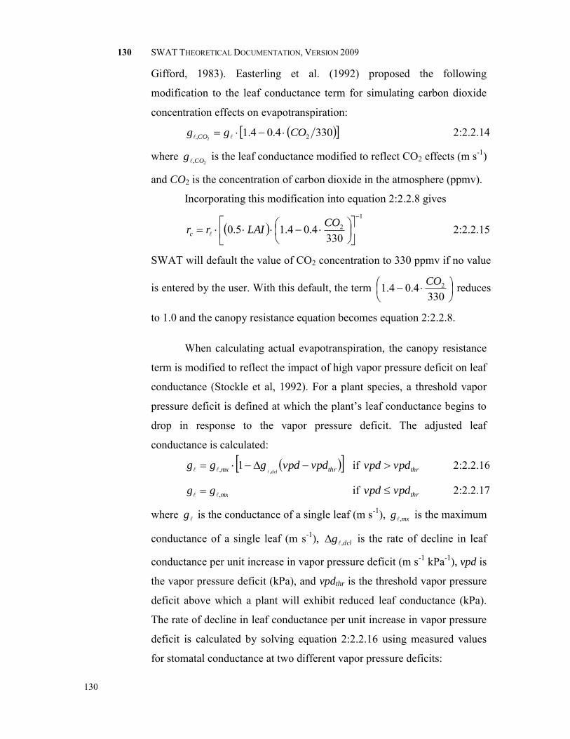
130 SWAT THEORETICAL DOCUMENTATION, VERSION 2009
130
Gifford, 1983). Easterling et al. (1992) proposed the following
modification to the leaf conductance term for simulating carbon dioxide
concentration effects on evapotranspiration:
3304.04.1 2, 2COgg CO 2:2.2.14
where 2,COg is the leaf conductance modified to reflect CO2 effects (m s-1)
and CO2 is the concentration of carbon dioxide in the atmosphere (ppmv).
Incorporating this modification into equation 2:2.2.8 gives
1
2
3304.04.15.0
CO
LAIrrc 2:2.2.15
SWAT will default the value of CO2 concentration to 330 ppmv if no value
is entered by the user. With this default, the term
3304.04.1 2CO reduces
to 1.0 and the canopy resistance equation becomes equation 2:2.2.8.
When calculating actual evapotranspiration, the canopy resistance
term is modified to reflect the impact of high vapor pressure deficit on leaf
conductance (Stockle et al, 1992). For a plant species, a threshold vapor
pressure deficit is defined at which the plant’s leaf conductance begins to
drop in response to the vapor pressure deficit. The adjusted leaf
conductance is calculated:
thrmx vpdvpdgggdcl
,
1, if thrvpdvpd 2:2.2.16
mxgg , if thrvpdvpd 2:2.2.17
where g is the conductance of a single leaf (m s-1), mxg , is the maximum
conductance of a single leaf (m s-1), dclg , is the rate of decline in leaf
conductance per unit increase in vapor pressure deficit (m s-1 kPa-1), vpd is
the vapor pressure deficit (kPa), and vpdthr is the threshold vapor pressure
deficit above which a plant will exhibit reduced leaf conductance (kPa).
The rate of decline in leaf conductance per unit increase in vapor pressure
deficit is calculated by solving equation 2:2.2.16 using measured values
for stomatal conductance at two different vapor pressure deficits:
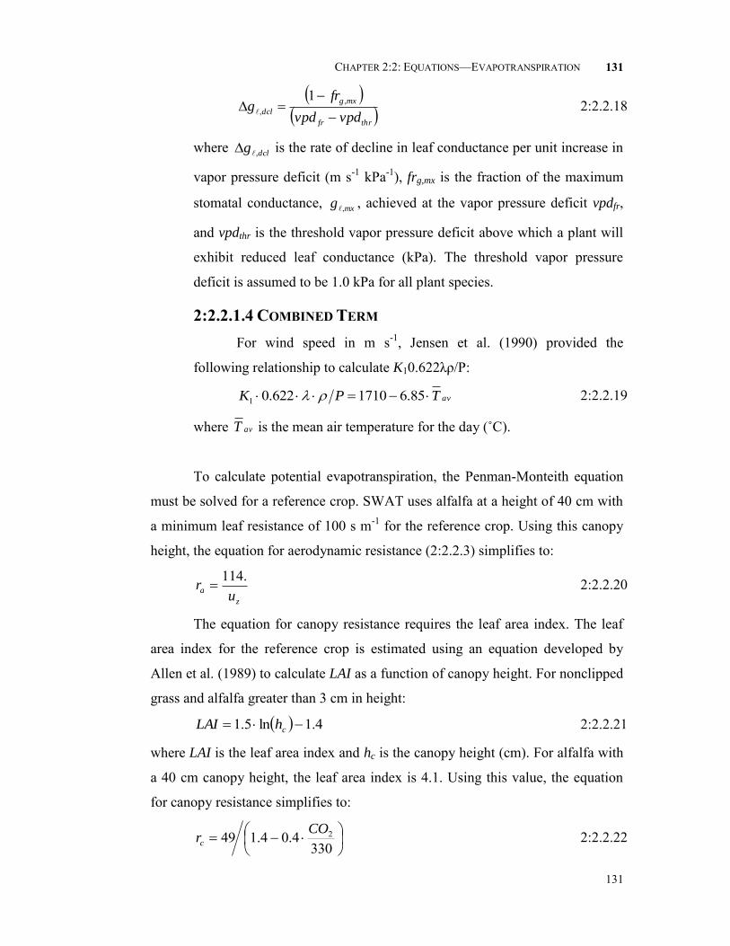
CHAPTER 2:2: EQUATIONS—EVAPOTRANSPIRATION
131
131
thrfr
mxg
dclvpdvpd
frg
,,
1 2:2.2.18
where dclg , is the rate of decline in leaf conductance per unit increase in
vapor pressure deficit (m s-1 kPa-1), frg,mx is the fraction of the maximum
stomatal conductance, mxg , , achieved at the vapor pressure deficit vpdfr,
and vpdthr is the threshold vapor pressure deficit above which a plant will
exhibit reduced leaf conductance (kPa). The threshold vapor pressure
deficit is assumed to be 1.0 kPa for all plant species.
2:2.2.1.4 COMBINED TERM For wind speed in m s-1, Jensen et al. (1990) provided the
following relationship to calculate K10.622λρ/P:
avTPK 85.61710622.01 2:2.2.19
where avT is the mean air temperature for the day (˚C).
To calculate potential evapotranspiration, the Penman-Monteith equation
must be solved for a reference crop. SWAT uses alfalfa at a height of 40 cm with
a minimum leaf resistance of 100 s m-1 for the reference crop. Using this canopy
height, the equation for aerodynamic resistance (2:2.2.3) simplifies to:
z
au
r.114
2:2.2.20
The equation for canopy resistance requires the leaf area index. The leaf
area index for the reference crop is estimated using an equation developed by
Allen et al. (1989) to calculate LAI as a function of canopy height. For nonclipped
grass and alfalfa greater than 3 cm in height:
4.1ln5.1 chLAI 2:2.2.21
where LAI is the leaf area index and hc is the canopy height (cm). For alfalfa with
a 40 cm canopy height, the leaf area index is 4.1. Using this value, the equation
for canopy resistance simplifies to:
3304.04.149 2CO
rc 2:2.2.22
132 SWAT THEORETICAL DOCUMENTATION, VERSION 2009
132
The most accurate estimates of evapotranspiration with the Penman-
Monteith equation are made when evapotranspiration is calculated on an hourly
basis and summed to obtain the daily values. Mean daily parameter values have
been shown to provide reliable estimates of daily evapotranspiration values and
this is the approach used in SWAT. However, the user should be aware that
calculating evapotranspiration with the Penman-Monteith equation using mean
daily values can potentially lead to significant errors. These errors result from
diurnal distributions of wind speed, humidity, and net radiation that in
combination create conditions which the daily averages do not replicate.
2:2.2.2 PRIESTLEY-TAYLOR METHOD Priestley and Taylor (1972) developed a simplified version of the
combination equation for use when surface areas are wet. The aerodynamic
component was removed and the energy component was multiplied by a
coefficient, pet = 1.28, when the general surroundings are wet or under humid
conditions
GHE netpeto
2:2.2.23
where λ is the latent heat of vaporization (MJ kg-1), Eo is the potential
evapotranspiration (mm d-1), pet is a coefficient, Δ is the slope of the saturation
vapor pressure-temperature curve, de/dT (kPa ˚C-1), γ is the psychrometric
constant (kPa ˚C-1), Hnet is the net radiation (MJ m-2 d-1), and G is the heat flux
density to the ground (MJ m-2 d-1).
The Priestley-Taylor equation provides potential evapotranspiration
estimates for low advective conditions. In semiarid or arid areas where the
advection component of the energy balance is significant, the Priestley-Taylor
equation will underestimate potential evapotranspiration.
2:2.2.3 HARGREAVES METHOD The Hargreaves method was originally derived from eight years of cool-
season Alta fescue grass lysimeter data from Davis, California (Hargreaves,

CHAPTER 2:2: EQUATIONS—EVAPOTRANSPIRATION
133
133
1975). Several improvements were made to the original equation (Hargreaves and
Samani, 1982 and 1985) and the form used in SWAT was published in 1985
(Hargreaves et al., 1985):
8.170023.0 5.00 avmnmxo TTTHE 2:2.2.24
where λ is the latent heat of vaporization (MJ kg-1), Eo is the potential
evapotranspiration (mm d-1), H0 is the extraterrestrial radiation (MJ m-2 d-1), Tmx is
the maximum air temperature for a given day (C), Tmn is the minimum air
temperature for a given day (C), and avT is the mean air temperature for a given
day (C).
Table 2:2-2: SWAT input variables used in potential evapotranspiration calculations summarized in this section.
Variable name
Definition
File Name
IPET Potential evapotranspiration method .bsn WND_SP uz: Daily wind speed (m/s) .wnd CO2 CO2: Carbon dioxide concentration (ppmv) .sub MAX TEMP Tmx: Daily maximum temperature (C) .tmp MIN TEMP Tmn: Daily minimum temperature (C) .tmp GSI
mxg , : maximum leaf conductance (m s-1) crop.dat
FRGMAX frg,mx: Fraction of maximum leaf conductance achieved at the vapor pressure deficit specified by vpdfr
crop.dat
VPDFR vpdfr: Vapor pressure deficit corresponding to value given for frg,mx (kPa)
crop.dat

134 SWAT THEORETICAL DOCUMENTATION, VERSION 2009
134
2:2.3 ACTUAL EVAPOTRANSPIRATION Once total potential evapotranspiration is determined, actual evaporation
must be calculated. SWAT first evaporates any rainfall intercepted by the plant
canopy. Next, SWAT calculates the maximum amount of transpiration and the
maximum amount of sublimation/soil evaporation using an approach similar to
that of Richtie (1972). The actual amount of sublimation and evaporation from the
soil is then calculated. If snow is present in the HRU, sublimation will occur.
Only when no snow is present will evaporation from the soil take place.
2:2.3.1 EVAPORATION OF INTERCEPTED RAINFALL Any free water present in the canopy is readily available for removal by
evapotranspiration. The amount of actual evapotranspiration contributed by
intercepted rainfall is especially significant in forests where in some instances
evaporation of intercepted rainfall is greater than transpiration.
SWAT removes as much water as possible from canopy storage when
calculating actual evaporation. If potential evapotranspiration, Eo, is less than the
amount of free water held in the canopy, RINT, then
ocana EEE 2:2.3.1
caniINTfINT ERR )()( 2:2.3.2
where Ea is the actual amount of evapotranspiration occurring in the watershed on
a given day (mm H2O), Ecan is the amount of evaporation from free water in the
canopy on a given day (mm H2O), Eo is the potential evapotranspiration on a
given day (mm H2O), RINT(i) is the initial amount of free water held in the canopy
on a given day (mm H2O), and RINT(f) is the final amount of free water held in the
canopy on a given day (mm H2O). If potential evapotranspiration, Eo, is greater
than the amount of free water held in the canopy, RINT, then
)(iINTcan RE 2:2.3.3
0)( fINTR 2:2.3.4

CHAPTER 2:2: EQUATIONS—EVAPOTRANSPIRATION
135
135
Once any free water in the canopy has been evaporated, the remaining
evaporative water demand ( canoo EEE ) is partitioned between the vegetation
and snow/soil.
2:2.3.2 TRANSPIRATION If the Penman-Monteith equation is selected as the potential
evapotranspiration method, transpiration is also calculated with the equations
summarized in Section 2:2.2.1. For the other potential evapotranspiration
methods, transpiration is calculated as:
0.3LAIE
E ot
0.30 LAI 2:2.3.5
ot EE 0.3LAI 2:2.3.6
where Et is the maximum transpiration on a given day (mm H2O), oE is the
potential evapotranspiration adjusted for evaporation of free water in the canopy
(mm H2O), and LAI is the leaf area index. The value for transpiration calculated
by equations 2:2.3.5 and 2:2.3.6 is the amount of transpiration that will occur on a
given day when the plant is growing under ideal conditions. The actual amount of
transpiration may be less than this due to lack of available water in the soil
profile. Calculation of actual plant water uptake and transpiration is reviewed in
Chapters 5:2 and 5:3.
2:2.3.3 SUBLIMATION AND EVAPORATION FROM THE SOIL The amount of sublimation and soil evaporation will be impacted by the
degree of shading. The maximum amount of sublimation/soil evaporation on a
given day is calculated as:
solos covEE 2:2.3.7
where Es is the maximum sublimation/soil evaporation on a given day (mm H2O),
oE is the potential evapotranspiration adjusted for evaporation of free water in the
canopy (mm H2O), and covsol is the soil cover index. The soil cover index is
calculated
CVcovsol 5100.5exp 2:2.3.8

136 SWAT THEORETICAL DOCUMENTATION, VERSION 2009
136
where CV is the aboveground biomass and residue (kg ha-1). If the snow water
content is greater than 0.5 mm H2O, the soil cover index is set to 0.5.
The maximum amount of sublimation/soil evaporation is reduced during
periods of high plant water use with the relationship:
ts
osss
EE
EEEE ,min 2:2.3.9
where sE is the maximum sublimation/soil evaporation adjusted for plant water
use on a given day (mm H2O), Es is the maximum sublimation/soil evaporation on
a given day (mm H2O), oE is the potential evapotranspiration adjusted for
evaporation of free water in the canopy (mm H2O), and Et is the transpiration on a
given day (mm H2O). When Et is low ss EE . However, as Et approaches oE ,
sol
ss
cov
EE
1.
2:2.3.3.1 SUBLIMATION Once the maximum amount of sublimation/soil evaporation for the
day is calculated, SWAT will first remove water from the snow pack to
meet the evaporative demand. If the water content of the snow pack is
greater than the maximum sublimation/soil evaporation demand, then
ssub EE 2:2.3.10
sif ESNOSNO )()( 2:2.3.11
.0sE 2:2.3.12
where Esub is the amount of sublimation on a given day (mm H2O), sE is
the maximum sublimation/soil evaporation adjusted for plant water use on
a given day (mm H2O), SNO(i) is the amount of water in the snow pack on
a given day prior to accounting for sublimation (mm H2O), SNO(f) is the
amount of water in the snow pack on a given day after accounting for
sublimation (mm H2O), and sE is the maximum soil water evaporation on

CHAPTER 2:2: EQUATIONS—EVAPOTRANSPIRATION
137
137
a given day (mm H2O). If the water content of the snow pack is less than
the maximum sublimation/soil evaporation demand, then
)(isub SNOE 2:2.3.13
.0)( fSNO 2:2.3.14
subss EEE 2:2.3.15
2:2.3.3.2 SOIL WATER EVAPORATION When an evaporation demand for soil water exists, SWAT must
first partition the evaporative demand between the different layers. The
depth distribution used to determine the maximum amount of water
allowed to be evaporated is:
zz
zEE szsoil
00713.0374.2exp, 2:2.3.16
where Esoil,z is the evaporative demand at depth z (mm H2O), sE is the
maximum soil water evaporation on a given day (mm H2O), and z is the
depth below the surface. The coefficients in this equation were selected so
that 50% of the evaporative demand is extracted from the top 10 mm of
soil and 95% of the evaporative demand is extracted from the top 100 mm
of soil.
The amount of evaporative demand for a soil layer is determined
by taking the difference between the evaporative demands calculated at
the upper and lower boundaries of the soil layer:
zusoilzlsoillysoil EEE ,,, 2:2.3.16
where Esoil,ly is the evaporative demand for layer ly (mm H2O), Esoil,zl is the
evaporative demand at the lower boundary of the soil layer (mm H2O),
and Esoil,zu is the evaporative demand at the upper boundary of the soil
layer (mm H2O).
Figure 2:2-1 graphs the depth distribution of the evaporative
demand for a soil that has been partitioned into 1 mm layers assuming a
total soil evaporation demand of 100 mm.

138 SWAT THEORETICAL DOCUMENTATION, VERSION 2009
138
Figure 2:2-1: Soil evaporative demand distribution with depth.
As mentioned previously, the depth distribution assumes 50% of
the evaporative demand is met by soil water stored in the top 10 mm of the
soil profile. With our example of a 100 mm total evaporative demand, 50
mm of water is 50%. This is a demand that the top layer cannot satisfy.
SWAT does not allow a different layer to compensate for the
inability of another layer to meet its evaporative demand. The evaporative
demand not met by a soil layer results in a reduction in actual
evapotranspiration for the HRU.
A coefficient has been incorporated into equation 2:2.3.16 to allow
the user to modify the depth distribution used to meet the soil evaporative
demand. The modified equation is:
escoEEE zusoilzlsoillysoil ,,, 2:2.3.17
where Esoil,ly is the evaporative demand for layer ly (mm H2O), Esoil,zl is the
evaporative demand at the lower boundary of the soil layer (mm H2O),
Esoil,zu is the evaporative demand at the upper boundary of the soil layer
0.00
1.00
2.00
3.00
4.00
5.00
6.00
7.00
8.00
9.00
1 51 101 151 201 251 301 351 401 451
Max
imu
m E
vap
ora
tio
n (
mm
H2O
)
Depth (mm)
Evaporation allowed with depth assuming 100 mm demand

CHAPTER 2:2: EQUATIONS—EVAPOTRANSPIRATION
139
139
(mm H2O), and esco is the soil evaporation compensation coefficient.
Solutions to this equation for different values of esco are graphed in
Figure 7-2. The plot for esco = 1.0 is that shown in Figure 2:2-1.
Figure 2:2-2: Soil evaporative demand distribution with depth
As the value for esco is reduced, the model is able to extract more
of the evaporative demand from lower levels.
When the water content of a soil layer is below field capacity, the
evaporative demand for the layer is reduced according to the following
equations:
lyly
lyly
lysoillysoilWPFC
FCSWEE
5.2exp,, when lyly FCSW 2:2.3.18
lysoillysoil EE ,, when lyly FCSW 2:2.3.19
where lysoilE , is the evaporative demand for layer ly adjusted for water
content (mm H2O), Esoil,ly is the evaporative demand for layer ly (mm
0.00
5.00
10.00
15.00
20.00
25.00
30.00
35.00
1 51 101 151 201 251 301 351 401 451
Maxim
um
Evap
ora
tio
n (
mm
H2O
)
Depth (mm)
Evaporation allowed with depth assuming 100 mm demand
esco = 1.0 esco = 0.9 esco = 0.8 esco = 0.7

140 SWAT THEORETICAL DOCUMENTATION, VERSION 2009
140
H2O), SWly is the soil water content of layer ly (mm H2O), FCly is the
water content of layer ly at field capacity (mm H2O), and WPly is the water
content of layer ly at wilting point (mm H2O).
In addition to limiting the amount of water removed by
evaporation in dry conditions, SWAT defines a maximum value of water
that can be removed at any time. This maximum value is 80% of the plant
available water on a given day where the plant available water is defined
as the total water content of the soil layer minus the water content of the
soil layer at wilting point (-1.5 MPa).
)(8.0min ,, lylylysoillysoil WPSWEE 2:2.3.20
where lysoilE , is the amount of water removed from layer ly by evaporation
(mm H2O), lysoilE , is the evaporative demand for layer ly adjusted for
water content (mm H2O), SWly is the soil water content of layer ly (mm
H2O), and WPly is the water content of layer ly at wilting point (mm H2O).
Table 2:2-3: SWAT input variables used in soil evaporation calculations. Variable
name
Definition File
Name ESCO esco: soil evaporation compensation coefficient .bsn, .hru
2:2.4 NOMENCLATURE CO2 Concentration of carbon dioxide in the atmosphere (ppmv) CV Total aboveground biomass and residue present on current day (kg ha-1) E Depth rate evaporation (mm d-1) Ea Actual amount of evapotranspiration on a given day (mm H2O) Ecan Amount of evaporation from free water in the canopy on a given day (mm H2O) Eo Potential evapotranspiration (mm d-1)
oE Potential evapotranspiration adjusted for evaporation of free water in the canopy (mm H2O)
Es Maximum sublimation/soil evaporation on a given day (mm H2O) sE Maximum sublimation/soil evaporation adjusted for plant water use on a given
day (mm H2O) sE Maximum soil water evaporation on a given day (mm H2O)
Esoil,ly Evaporative demand for layer ly (mm H2O)

CHAPTER 2:2: EQUATIONS—EVAPOTRANSPIRATION
141
141
lysoilE , Evaporative demand for layer ly adjusted for water content (mm H2O)
lysoilE , Amount of water removed from layer ly by evaporation (mm H2O) Esoil,z Evaporative demand at depth z (mm H2O) Esub Amount of sublimation on a given day (mm H2O) Et Transpiration rate (mm d-1) FCly Water content of layer ly at field capacity (mm H2O) G Heat flux density to the ground (MJ m-2 d-1) H0 Extraterrestrial daily irradiation (MJ m-2 d-1) Hnet Net radiation on day (MJ m-2 d-1) K1 Dimension coefficient in Penman-Monteith equation
LAI Leaf area index of the canopy
LAImx Maximum leaf area index for the plant P Atmospheric pressure (kPa) Rday Amount of rainfall on a given day (mm H2O)
dayR Amount of precipitation on a given day before canopy interception is removed (mm H2O)
RINT Amount of free water held in the canopy on a given day (mm H2O) SNO Water content of snow cover on current day (mm H2O) SWly Soil water content of layer ly (mm H2O) Tmn Minimum air temperature for day (C) Tmx Maximum air temperature for day (C)
avT Mean air temperature for day (C) WPly Water content of layer ly at wilting point (mm H2O).
cp Specific heat of moist air at constant pressure (1.013 10-3 MJ kg-1 C-1) canday Maximum amount of water that can be trapped in the canopy on a given day (mm
H2O) canmx Maximum amount of water that can be trapped in the canopy when the canopy is
fully developed (mm H2O) covsol Soil cover index d Zero plane displacement of the wind profile (cm) e Actual vapor pressure on a given day (kPa)
oe Saturation vapor pressure on a given day (kPa) esco Soil evaporation compensation coefficient frg,mx Fraction of the maximum stomatal conductance, mxg , , achieved at the vapor
pressure deficit, vpdfr g Leaf conductance (m s-1)
mxg , Maximum conductance of a single leaf (m s-1) hc Canopy height (cm) k Von Kármán constant ra Diffusion resistance of the air layer (aerodynamic resistance) (s m-1) rc Plant canopy resistance (s m-1) r Minimum effective resistance of a single leaf (s m-1)

142 SWAT THEORETICAL DOCUMENTATION, VERSION 2009
142
abr Minimum abaxial stomatal leaf resistance (s m-1)
adr Minimum adaxial stomatal leaf resistance (s m-1) uz Wind speed at height zw (m s-1) vpd Vapor pressure deficit (kPa) vpdfr Vapor pressure deficit corresponding to frg,mx (kPa) vpdthr Threshold vapor pressure deficit above which a plant will exhibit reduced leaf
conductance (kPa) z Depth below soil surface (mm) zom Roughness length for momentum transfer (cm) zov Roughness length for vapor transfer (cm) zp Height of the humidity (psychrometer) and temperature measurements (cm) zw Height of the wind speed measurement (cm) pet Coefficient in Priestley-Taylor equation
Slope of the saturation vapor pressure curve (kPa C-1) dclg , Rate of decline in leaf conductance per unit increase in vapor pressure deficit (m
s-1 kPa-1) ρair Air density (kg m-3) Psychrometric constant (kPa C-1) Latent heat of vaporization (MJ kg-1)
2:2.5 REFERENCES
Allen, R.G. 1986. A Penman for all seasons. J. Irrig. and Drain Engng., ASCE,
112(4): 348-368.
Allen, R.G., M.E. Jensen, J.L. Wright, and R.D. Burman. 1989. Operational
estimates of evapotranspiration. Agron. J. 81:650-662.
Brutsaert, W. 1975. Comments on surface roughness parameters and the height of
dense vegetation. J. Meterol. Soc. Japan 53:96-97.
Dingman, S.L. 1994. Physical hydrology. Prentice-Hall, Inc., Englewood Cliffs,
NJ.
Easterling, W.E., N.J. Rosenburg, M.S. McKenney, C.A. Jones, P.T. Dyke, and
J.R. Williams. 1992. Preparing the erosion productivity impact calculator
(EPIC) model to simulate crop response to climate change and the direct
effects of CO2. Agricultural and Forest Meteorology 59:17-34.

CHAPTER 2:2: EQUATIONS—EVAPOTRANSPIRATION
143
143
Hargreaves, G.H. 1975. Moisture availability and crop production. Trans. ASAE
18: 980-984.
Hargreaves, G.H. and Z.A. Samani. 1985. Reference crop evapotranspiration from
temperature. Applied Engineering in Agriculture 1:96-99.
Hargreaves, G.H. and Z.A. Samani. 1982. Estimating potential evapotranspir-
ation. Tech. Note, J. Irrig. and Drain. Engr. 108(3):225-230.
Hargreaves, G.L., G.H. Hargreaves, and J.P. Riley. 1985. Agricultural benefits for
Senegal River Basin. J. Irrig. and Drain. Engr. 111(2):113-124.
Jensen, M.E., R.D. Burman, and R.G. Allen (ed). 1990. Evapotranspiration and
irrigation water requirements. ASCE Manuals and Reports on Engineering
Practice No. 70, ASCE, N.Y. 332 pp.
Monteith, J.L. 1965. Evaporation and the environment. p. 205-234. In The state
and movement of water in living organisms, XIXth Symposium. Soc. for
Exp. Biol., Swansea, Cambridge University Press.
Monteith, J.L. 1981. Evaporation and surface temperature. Quart. J. Roy.
Meteorol. Soc. 107:1-27.
Morison, J.I.L. 1987. Intercellular CO2 concentration and stomatal response to
CO2. p. 229-251. In E. Zeiger, G.D. Farquhar and I.R. Cowan (ed.)
Stomatal function. Standford University Press, Palo Alto, CA.
Morison, J.I.L. and R.M. Gifford. 1983. Stomatal sensitivity tocarbon dioxide and
humidity. Plant Physiol. 71:789-796.
Penman, H.L. 1956. Evaporation: An introductory survey. Netherlands Journal of
Agricultural Science 4:7-29.
Plate, E.J. 1971. Aerodynamic characteristics of atmospheric boundary layers.
U.S. Atomic Energy Comm., Critical Review Series, TID-25465. 190 pp.
Priestley, C.H.B. and R.J. Taylor. 1972. On the assessment of surface heat flux
and evaporation using large-scale parameters. Mon. Weather. Rev.
100:81-92.
Ritchie, J.T. 1972. Model for predicting evaporation from a row crop with
incomplete cover. Water Resour. Res. 8:1204-1213.

144 SWAT THEORETICAL DOCUMENTATION, VERSION 2009
144
Rosenburg, N.J., B.L. Blad, and S.B. Verma. 1983. Microclimate: the biological
environment, 2nd ed. John Wiley & Sons, New York.
Stockle, C.O., J.R. Williams, N.J. Rosenberg, and C.A. Jones. 1992. A method for
estimating the direct and climatic effects of rising atmospheric carbon
dioxide on growth and yield of crops: Part 1—Modification of the EPIC
model for climate change analysis. Agricultural Systems 38:225-238.
Stricker, H. and W. Brutsaert. 1978. Actual evapotranspiration over summer
period in the 'Hupsel Catchment.' J. Hydrol. 39:139-157.
Thornthwaite, C.W. 1948. An approach toward a rational classification of climate.
Geographical Review 38:55-94.

CHAPTER 2:2: EQUATIONS—EVAPOTRANSPIRATION
145
145

146
SECTION 2 CHAPTER 3
EQUATIONS: SOIL WATER
Water that enters the soil may move along one of several different
pathways. The water may be removed from the soil by plant uptake or
evaporation. It can percolate past the bottom of the soil profile and ultimately
become aquifer recharge. A final option is that water may move laterally in the
profile and contribute to streamflow. Of these different pathways, plant uptake of
water removes the majority of water that enters the soil profile.

CHAPTER 2:3: EQUATIONS—SOIL WATER
147
147
2:3.1 SOIL STRUCTURE Soil is comprised of three phases—solid, liquid and gas. The solid phase
consists of minerals and/or organic matter that forms the matrix or skeleton of the
soil. Between the solid particles, soil pores are formed that hold the liquid and gas
phases. The soil solution may fill the soil pores completely (saturated) or partially
(unsaturated). When the soil is unsaturated, the soil solution is found as thin films
along particle surfaces, as annular wedges around contact points of particles and
as isolated bodies in narrow pore passages.
The soil’s bulk density defines the relative amounts of pore space and soil
matrix. Bulk density is calculated:
T
Sb
V
M 2:3.1.1
where b is the bulk density (Mg m-3), MS is the mass of the solids (Mg), and VT is
the total volume (m3). The total volume is defined as
SWAT VVVV 2:3.1.2
where VA is the volume of air (m3), VW is the volume of water (m3), and VS is the
volume of solids (m3). The relationship between soil porosity and soil bulk
density is
s
bsoil
1 2:3.1.3
where soil is the soil porosity expressed as a fraction of the total soil volume, b is
the bulk density (Mg m-3), and s is the particle density (Mg m-3). The particle
density, or density of the solid fraction, is a function of the mineral composition
of the soil matrix. Based on research, a default value of 2.65 Mg m-3 is used for
particle density.
Storage, transport and availability of soil solution and soil air are not
nearly as dependent on the total amount of porosity as they are on the
arrangement of pore space. Soil pores vary in size and shape due to textural and
structural arrangement. Based on the diameter of the pore at the narrowest point,
the pores may be classified as macropores (narrowest diameter > 100 m),
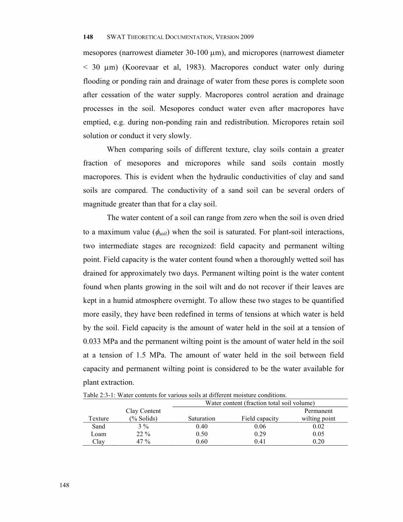
148 SWAT THEORETICAL DOCUMENTATION, VERSION 2009
148
mesopores (narrowest diameter 30-100 m), and micropores (narrowest diameter
< 30 m) (Koorevaar et al, 1983). Macropores conduct water only during
flooding or ponding rain and drainage of water from these pores is complete soon
after cessation of the water supply. Macropores control aeration and drainage
processes in the soil. Mesopores conduct water even after macropores have
emptied, e.g. during non-ponding rain and redistribution. Micropores retain soil
solution or conduct it very slowly.
When comparing soils of different texture, clay soils contain a greater
fraction of mesopores and micropores while sand soils contain mostly
macropores. This is evident when the hydraulic conductivities of clay and sand
soils are compared. The conductivity of a sand soil can be several orders of
magnitude greater than that for a clay soil.
The water content of a soil can range from zero when the soil is oven dried
to a maximum value (soil) when the soil is saturated. For plant-soil interactions,
two intermediate stages are recognized: field capacity and permanent wilting
point. Field capacity is the water content found when a thoroughly wetted soil has
drained for approximately two days. Permanent wilting point is the water content
found when plants growing in the soil wilt and do not recover if their leaves are
kept in a humid atmosphere overnight. To allow these two stages to be quantified
more easily, they have been redefined in terms of tensions at which water is held
by the soil. Field capacity is the amount of water held in the soil at a tension of
0.033 MPa and the permanent wilting point is the amount of water held in the soil
at a tension of 1.5 MPa. The amount of water held in the soil between field
capacity and permanent wilting point is considered to be the water available for
plant extraction. Table 2:3-1: Water contents for various soils at different moisture conditions.
Water content (fraction total soil volume)
Texture Clay Content
(% Solids)
Saturation
Field capacity Permanent
wilting point Sand 3 % 0.40 0.06 0.02 Loam 22 % 0.50 0.29 0.05 Clay 47 % 0.60 0.41 0.20

CHAPTER 2:3: EQUATIONS—SOIL WATER
149
149
Table 2:3-1 lists the water content for three soils as a fraction of the total
volume for different moisture conditions. Note that the total porosity, given by the
water content at saturation, is lowest for the sand soil and highest for the clay soil.
The sand soil drains more quickly than the loam and clay. Only 15% of
the water present in the sand soil at saturation remains at field capacity. 58% of
the water present at saturation in the loam remains at field capacity while 68% of
the water present at saturation in the clay soil remains at field capacity. The
reduction of water loss with increase in clay content is cause by two factors. As
mentioned previously, clay soils contain more mesopores and micropores than
sand soils. Also, unlike sand and silt particles, clay particles possess a net
negative charge. Due to the polar nature of water molecules, clay particles are
able to attract and retain water molecules. The higher water retention of clay soils
is also seen in the fraction of water present at permanent wilting point. In the soils
listed in Table 2:3-1, the volumetric water content of the clay is 0.20 at the wilting
point while the sand and loam have a volumetric water content of 0.02 and 0.05
respectively.
The plant available water, also referred to as the available water capacity,
is calculated by subtracting the fraction of water present at permanent wilting
point from that present at field capacity.
WPFCAWC 2:3.1.4
where AWC is the plant available water content, FC is the water content at field
capacity, and WP is the water content at permanent wilting point. For the three
soil textures listed in Table 2:3-1, the sand has an available water capacity of
0.04, the loam has an available water capacity of 0.24 and the clay has an
available water capacity of 0.21. Even though the clay contains a greater amount
of water than the loam at all three tensions, the loam has a larger amount of water
available for plant uptake than the clay. This characteristic is true in general.
SWAT estimates the permanent wilting point volumetric water content for
each soil layer as:
100
40.0 bcly
mWP
2:3.1.5

150 SWAT THEORETICAL DOCUMENTATION, VERSION 2009
150
where WPly is the water content at wilting point expressed as a fraction of the total
soil volume, mc is the percent clay content of the layer (%), and b is the bulk
density for the soil layer (Mg m-3). Field capacity water content is estimated
lylyly AWCWPFC 2:3.1.6
where FCly is the water content at field capacity expressed as a fraction of the
total soil volume, WPly is the water content at wilting point expressed as a fraction
of the total soil volume, and AWCly is the available water capacity of the soil layer
expressed as a fraction of the total soil volume. AWCly is input by the user.
Water in the soil can flow under saturated or unsaturated conditions. In
saturated soils, flow is driven by gravity and usually occurs in the downward
direction. Unsaturated flow is caused by gradients arising due to adjacent areas of
high and low water content. Unsaturated flow may occur in any direction.
SWAT directly simulates saturated flow only. The model records the
water contents of the different soil layers but assumes that the water is uniformly
distributed within a given layer. This assumption eliminates the need to model
unsaturated flow in the horizontal direction. Unsaturated flow between layers is
indirectly modeled with the depth distribution of plant water uptake (equation
5:2.2.1) and the depth distribution of soil water evaporation (equation 2:2.3.16).
Saturated flow occurs when the water content of a soil layer surpasses the
field capacity for the layer. Water in excess of the field capacity water content is
available for percolation, lateral flow or tile flow drainage unless the temperature
of the soil layer is below 0C. When the soil layer is frozen, no water movement
is calculated.
Table 2:3-1: SWAT input variables used in percolation calculations. Variable
name
Definition File
Name CLAY mc: Percent clay content .sol SOL_BD b: Bulk density (Mg m-3) .sol SOL_AWC AWCly: available water capacity .sol

CHAPTER 2:3: EQUATIONS—SOIL WATER
151
151
2:3.2 PERCOLATION
Percolation is calculated for each soil layer in the profile. Water is allowed
to percolate if the water content exceeds the field capacity water content for that
layer and the layer below is not saturated. When the soil layer is frozen, no water
flow out of the layer is calculated.
The volume of water available for percolation in the soil layer is
calculated:
lylyexcessly FCSWSW , if
lyly FCSW 2:3.2.1
0, excesslySW if lyly FCSW 2:3.2.2
where SWly,excess is the drainable volume of water in the soil layer on a given day
(mm H2O), SWly is the water content of the soil layer on a given day (mm H2O)
and FCly is the water content of the soil layer at field capacity (mm H2O).
The amount of water that moves from one layer to the underlying layer is
calculated using storage routing methodology. The equation used to calculate the
amount of water that percolates to the next layer is:
perc
excesslylypercTT
tSWw exp1,, 2:3.2.3
where wperc,ly is the amount of water percolating to the underlying soil
layer on a given day (mm H2O), SWly,excess is the drainable volume of water in the
soil layer on a given day (mm H2O), t is the length of the time step (hrs), and
TTperc is the travel time for percolation (hrs). If the HRU has a seasonal high water
table, percolation is not allowed when 1111 5.0 lylylyly FCSATFCSW
where SWly+1 is the water content of the underlying soil layer (mm H2O), FCly+1 is
the water content of the underlying soil layer at field capacity (mm H2O), and
SATly+1 is the amount of water in the underlying soil layer when completely
saturated (mm H2O). The water will instead stay ponded in the upper layer.
The travel time for percolation is unique for each layer. It is calculate
sat
lyly
percK
FCSATTT
2:3.2.4

152 SWAT THEORETICAL DOCUMENTATION, VERSION 2009
152
where TTperc is the travel time for percolation (hrs), SATly is the amount of water
in the soil layer when completely saturated (mm H2O), FCly is the water content
of the soil layer at field capacity (mm H2O), and Ksat is the saturated hydraulic
conductivity for the layer (mm∙h-1).
Water that percolates out of the lowest soil layer enters the vadose zone.
The vadose zone is the unsaturated zone between the bottom of the soil profile
and the top of the aquifer. Movement of water through the vadose zone and into
the aquifers is reviewed in Chapter 2:4.
Table 2:3-2: SWAT input variables used in percolation calculations. Variable
name
Definition File
Name SOL_K Ksat: Saturated hydraulic conductivity (mm/hr) .sol IWATABLE High water table code: 0-no water table in soil profile 1-seasonal high
water table present in profile .hru
2:3.3 BYPASS FLOW One of the most unique soil orders is the Vertisols. These soils are
characterized by a propensity to shrink when dried and swell when moistened.
When the soil is dry, large cracks form at the soil surface. This behavior is a result
of the type of soil material present and the climate. Vertisols contain at least 30%
clay with the clay fraction dominated by smectitic mineralogy and occur in areas
with cyclical wet and dry periods.
Vertisols are found worldwide (Figure 2:3-1). They have a number of
local names, some of which are listed in Table 2:3-3.

CHAPTER 2:3: EQUATIONS—SOIL WATER
153
153
Figure 2:3-1: Soil associations of Vertisols (After Dudal and Eswaran, 1988)
Table 2:3-3: Alternative names for Vertisols or soils with Vertic properties (Dudal and Eswaran, 1988).
Names Countries Names that include the word “black” Barros pretos Portugal Black clays South Africa, Australia Black cotton soils Africa, India Black cracking clays Uganda Black earths Australia, Africa Black turf soils South Africa Dark clay soils United States Subtropical black clays Africa Sols noirs tropicaux Africa Terra nera Italy Terres noires tropicales Africa Terras negras tropicais Mozambique Tierras negras de Andalucia Spain Tropical black earths Angola, Ghana Tropical black clays Africa Names that reflect the black color Karail India Melanites Ghana Teen Suda Sudan Tropical Chernozems Africa, India Impact Chernozems Russia Vernacular names Adobe soils United States, Philippines Badobes Sudan Dian Pere French West Africa Gilgai soils Australia Firki Nigeria Mbuga Tanzania Kahamba Congo Makande Malawi Morogan Romania Regur India Rendzina United States Shachiang soils China Smolnitza Bulgaria, Romania

154 SWAT THEORETICAL DOCUMENTATION, VERSION 2009
154
Table 2:3-3 Cont.
Names Countries Smonitza Austria, Yugoslavia Sols de paluds France Tirs Morocco, North Africa Vlei grond South Africa Sonsocuite Nicaragua Coined names Densinigra soils Angola Gravinigra soils Angola Grumusols United States Margalite soils Indonesia Vertisols United States
One criteria used to classify a soil as a Vertisol is the formation of
shrinkage cracks in the dry season that penetrate to a depth of more than 50 cm
and are at least 1 cm wide at 50 cm depth. The cracks can be considerably wider
at the surface—30 cm cracks at the surface are not unusual although 6-15 cm
cracks are more typical.
To accurately predict surface runoff and infiltration in areas dominated by
soils that exhibit Vertic properties, the temporal change in soil volume must be
quantified. Bouma and Loveday (1988) identified three soil moisture conditions
for which infiltration needs to be defined (Figure 2:3-2).
Figure 2:3-2: Diagram showing the effect of wetting and drying on cracking in Vertisols (After Bouma and Loveday, 1988)
Traditional models of infiltration are applicable to soils in which cracks
have been closed by swelling and the soil acts as a relatively homogenous porous
medium (Condition 3 in Figure 2:3-2). Condition 1 in Figure 2:3-2 represents the
CHAPTER 2:3: EQUATIONS—SOIL WATER
155
155
driest state with cracks at maximum width, a condition present at the end of the
dry season/beginning of the rainy season. Condition 2 in Figure 2:3-2 represents
the crack development typical with an actively growing crop requiring multiple
irrigation or rainfall events to sustain growth. Bypass flow, the vertical movement
of free water along macropores through unsaturated soil horizons, will occur in
conditions 1 and 2. Bypass flow (finf,2 in Figure 2:3-2) occurs when the rate of
rainfall or irrigation exceeds the vertical infiltration rate into the soil peds (finf,1 in
Figure 2:3-2).
When bypass flow is modeled, SWAT calculates the crack volume of the
soil matrix for each day of simulation by layer. On days in which precipitation
events occur, infiltration and surface runoff is first calculated for the soil peds
(finf,1 in Figure 2:3-2) using the curve number or Green & Ampt method. If any
surface runoff is generated, it is allowed to enter the cracks. A volume of water
equivalent to the total crack volume for the soil profile may enter the profile as
bypass flow. Surface runoff in excess of the crack volume remains overland flow.
Water that enters the cracks fills the soil layers beginning with the lowest
layer of crack development. After cracks in one layer are filled, the cracks in the
overlying layer are allowed to fill.
The crack volume initially estimated for a layer is calculated:
lycrk
lylycrk
lymaxilyFCcoef
SWFCcoefcrkcrk
,, 2:3.3.1
where crkly,i is the initial crack volume calculated for the soil layer on a given day
expressed as a depth (mm), crkmax,ly is the maximum crack volume possible for the
soil layer (mm), coefcrk is an adjustment coefficient for crack flow, FCly is the
water content of the soil layer at field capacity (mm H2O), and SWly is the water
content of the soil layer on a given day (mm H2O). The adjustment coefficient for
crack flow, coefcrk, is set to 0.10.
When the moisture content of the entire profile falls below 90% of the
field capacity water content for the profile during the drying stage, the crack
volume for a given day is a function of the crack volume estimated with equation

156 SWAT THEORETICAL DOCUMENTATION, VERSION 2009
156
2:3.3.1 and the crack volume of the layer on the previous day. When the soil is
wetting and/or when the moisture content of the profile is above 90% of the field
capacity water content, the crack volume for a given day is equal to the volume
calculated with equation 2:3.3.1.
ilycrkdlycrkly crkcrkcrk ,1, )0.1(
when FCSW 90.0 and 1,, dlyily crkcrk 2:3.3.2
ilyly crkcrk ,
when FCSW 90.0 or 1,, dlyily crkcrk 2:3.3.3
where crkly is the crack volume for the soil layer on a given day expressed as a
depth (mm), crk is the lag factor for crack development during drying, crkly,d-1 is
the crack volume for the soil layer on the previous day (mm), crkly,i is the initial
crack volume calculated for the soil layer on a given day using equation 2:3.3.1
(mm), SW is the water content of the soil profile on a given day (mm H2O), and
FC is the water content of the soil profile at field capacity (mm H2O).
As the tension at which water is held by the soil particles increases, the
rate of water diffusion slows. Because the rate of water diffusion is analogous to
the coefficient of consolidation in classical consolidation theory (Mitchell, 1992),
the reduction in diffusion will affect crack formation. The lag factor is introduced
during the drying stage to account for the change in moisture redistribution
dynamics that occurs as the soil dries. The lag factor, crk , is set to a value of
0.99.
The maximum crack volume for the layer, crkmax,ly, is calculated:
lylylmaxmax,ly depthzcrkcrk ,0012.0exp916.0 2:3.3.4
where crkmax,ly is the maximum crack volume possible for the soil layer (mm),
crkmax is the potential crack volume for the soil profile expressed as a fraction of
the total volume, zl,ly is the depth from the soil surface to the bottom of the soil
layer (mm), and depthly is the depth of the soil layer (mm). The potential crack
volume for the soil profile, crkmax, is input by the user. Those needing information
on the measurement of this parameter are referred to Bronswijk (1989; 1990).

CHAPTER 2:3: EQUATIONS—SOIL WATER
157
157
Once the crack volume for each layer is calculated, the total crack volume
for the soil profile is determined.
n
ly
lycrkcrk1
2:3.3.5
where crk is the total crack volume for the soil profile on a given day (mm), crkly
is the crack volume for the soil layer on a given day expressed as a depth (mm), ly
is the layer, and n is the number of layers in the soil profile.
After surface runoff is calculated for rainfall events using the curve
number or Green & Ampt method, the amount of runoff is reduced by the volume
of cracks present that day:
crkQQ isurfsurf , if crkQ isurf , 2:3.3.6
0surfQ if crkQ isurf , 2:3.3.7
where Qsurf is the accumulated runoff or rainfall excess for the day (mm H2O),
Qsurf,i is the initial accumulated runoff or rainfall excess determined with the
Green & Ampt or curve number method (mm H2O), and crk is the total crack
volume for the soil profile on a given day (mm). The total amount of water
entering the soil is then calculated:
surfdayinf QRw 2:3.3.8
where winf is the amount of water entering the soil profile on a given day (mm
H2O), Rday is the rainfall depth for the day adjusted for canopy interception (mm
H2O), and Qsurf is the accumulated runoff or rainfall excess for the day (mm H2O).
Bypass flow past the bottom of the profile is calculated:
nnly
nnly
btmcrkdepth
crkcrkw 5.0, 2:3.3.9
where wcrk,btm is the amount of water flow past the lower boundary of the soil
profile due to bypass flow (mm H2O), crk is the total crack volume for the soil
profile on a given day (mm), crkly=nn is the crack volume for the deepest soil layer
(ly=nn) on a given day expressed as a depth (mm), and depthly=nn is the depth of
the deepest soil layer (ly=nn) (mm).

158 SWAT THEORETICAL DOCUMENTATION, VERSION 2009
158
After wcrk,btm is calculated, each soil layer is filled to field capacity water
content beginning with the lowest layer and moving upward until the total amount
of water entering the soil, winf, has been accounted for.
Table 2:3-4: SWAT input variables used in bypass flow calculations. Variable
name
Definition File
Name ICRK Bypass flow code: 0-do not model bypass flow; 1-model bypass flow .bsn SOL_CRK crkmax: Potential crack volume for soil profile .sol
2:3.4 PERCHED WATER TABLE
For an HRU with a seasonal high water table, if the soil profile becomes
saturated to the point that percolation for upper soil layers to lower soil layers is
inhibited, water will pond in the soil profile and create a perched water table.
SWAT allows the user to define the depth to an impervious layer for the
HRU. If the depth to the impervious layer is in the soil profile, no water is
allowed to percolate out of the soil profile. If the impervious layer is defined
below the soil profile, percolation out of the soil profile is adjusted from the value
determined with equation 2:3.2.3 using:
diffdiff
diff
origbtmpercbtmpercdepthdepth
depthww
598.2833.8exp,,, 2:3.4.1
where wperc,btm is the amount of water percolating out of the soil profile on a given
day (mm H2O), wperc,btm,orig is the amount of water percolating out of the soil
profile on a given day calculated with equation 2:3.2.3 (mm H2O), and depthdiff is
the distance from the bottom of the soil profile to the impervious layer (m).
Water builds up in the soil profile from the bottom of the profile. After the
bottom layer of the profile reaches saturation, any water exceeding the storage
capacity of the bottom layer is allowed to fill the overlying layer. This continues
upward until all the excess water has been distributed.
The height of the perched water table is calculated:
imp
air
wtbl depthFCPOR
FCSWh
1 2:3.4.2

CHAPTER 2:3: EQUATIONS—SOIL WATER
159
159
where hwtbl is the height of the water table (mm), SW is the water content of the
soil profile (mm H2O), FC is the water content of the soil profile at field capacity
(mm H2O), POR is the porosity of the soil profile (mm), air is the air-filled
porosity expressed as a fraction, and depthimp is the depth to the impervious layer
(mm).
Table 2:3-5: SWAT input variables used in perched water table calculations. Variable
name
Definition File
Name DEP_IMP depthimp: Depth to impervious layer (mm) .hru DEPIMP_BSN depthimp: Depth to impervious layer (mm) .bsn
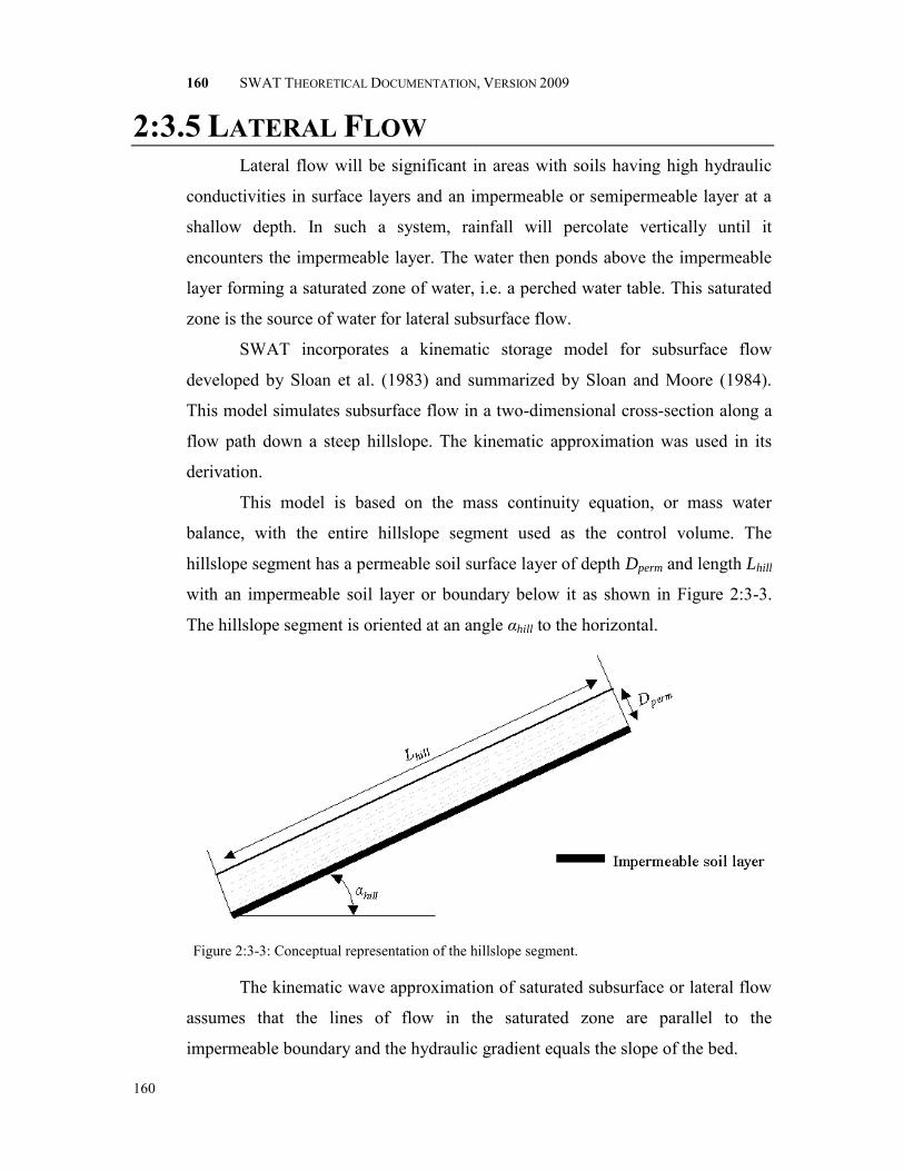
160 SWAT THEORETICAL DOCUMENTATION, VERSION 2009
160
2:3.5 LATERAL FLOW Lateral flow will be significant in areas with soils having high hydraulic
conductivities in surface layers and an impermeable or semipermeable layer at a
shallow depth. In such a system, rainfall will percolate vertically until it
encounters the impermeable layer. The water then ponds above the impermeable
layer forming a saturated zone of water, i.e. a perched water table. This saturated
zone is the source of water for lateral subsurface flow.
SWAT incorporates a kinematic storage model for subsurface flow
developed by Sloan et al. (1983) and summarized by Sloan and Moore (1984).
This model simulates subsurface flow in a two-dimensional cross-section along a
flow path down a steep hillslope. The kinematic approximation was used in its
derivation.
This model is based on the mass continuity equation, or mass water
balance, with the entire hillslope segment used as the control volume. The
hillslope segment has a permeable soil surface layer of depth Dperm and length Lhill
with an impermeable soil layer or boundary below it as shown in Figure 2:3-3.
The hillslope segment is oriented at an angle αhill to the horizontal.
Figure 2:3-3: Conceptual representation of the hillslope segment.
The kinematic wave approximation of saturated subsurface or lateral flow
assumes that the lines of flow in the saturated zone are parallel to the
impermeable boundary and the hydraulic gradient equals the slope of the bed.

CHAPTER 2:3: EQUATIONS—SOIL WATER
161
161
Figure 2:3-4: Behavior of the water table as assumed in the kinematic storage model.
From Figure 2:3-4, the drainable volume of water stored in the saturated
zone of the hillslope segment per unit area, SWly,excess, is
21000
,hilldo
excessly
LHSW
2:3.5.1
where SWly,excess is the drainable volume of water stored in the saturated zone of
the hillslope per unit area (mm H2O), Ho is the saturated thickness normal to the
hillslope at the outlet expressed as a fraction of the total thickness (mm/mm), d is
the drainable porosity of the soil (mm/mm), Lhill is the hillslope length (m), and
1000 is a factor needed to convert meters to millimeters. This equation can be
rearranged to solve for Ho:
hilld
excessly
oL
SWH
10002 , 2:3.5.2
The drainable porosity of the soil layer is calculated:
fcsoild 2:3.5.3
where d is the drainable porosity of the soil layer (mm/mm), soil is the total
porosity of the soil layer (mm/mm), and fc is the porosity of the soil layer filled
with water when the layer is at field capacity water content (mm/mm).

162 SWAT THEORETICAL DOCUMENTATION, VERSION 2009
162
A soil layer is considered to be saturated whenever the water content of
the layer exceeds the layer’s field capacity water content. The drainable volume
of water stored in the saturated layer is calculated:
lylyexcessly FCSWSW , if
lyly FCSW 2:3.5.4
0, excesslySW if lyly FCSW 2:3.5.5
where SWly is the water content of the soil layer on a given day (mm H2O) and
FCly is the water content of the soil layer at field capacity (mm H2O).
The net discharge at the hillslope outlet, Qlat, is given by
latolat vHQ 24 2:3.5.6
where Qlat is the water discharged from the hillslope outlet (mm H2O/day), Ho is
the saturated thickness normal to the hillslope at the outlet expressed as a fraction
of the total thickness (mm/mm), vlat is the velocity of flow at the outlet (mm∙h-1),
and 24 is a factor to convert hours to days.
Velocity of flow at the outlet is defined as
hillsatlat Kv sin 2:3.5.7
where Ksat is the saturated hydraulic conductivity (mm∙h-1) and hill is the slope of
the hillslope segment. The slope is input to SWAT as the increase in elevation per
unit distance (slp) which is equivalent to hilltan . Because hillhill sintan ,
equation 2:3.5.3 is modified to use the value for the slope as input to the model:
slpKKv sathillsatlat tan 2:3.5.8
Combining equations 2:3.5.2 and 2:3.5.8 with equation 2:3.5.6 yields the
equation
hilld
satexcessly
latL
slpKSWQ
,2024.0 2:3.5.9
where all terms are previously defined.
2:3.5.1 LATERAL FLOW LAG In large subbasins with a time of concentration greater than 1 day, only a
portion of the lateral flow will reach the main channel on the day it is generated.

CHAPTER 2:3: EQUATIONS—SOIL WATER
163
163
SWAT incorporates a lateral flow storage feature to lag a portion of lateral flow
release to the main channel.
Once lateral flow is calculated, the amount of lateral flow released to the
main channel is calculated:
lag
ilatstorlatlatTT
QQQ1exp11, 2:3.5.10
where Qlat is the amount of lateral flow discharged to the main channel on a given
day (mm H2O), latQ is the amount of lateral flow generated in the subbasin on a
given day (mm H2O), Qlatstor,i-1 is the lateral flow stored or lagged from the
previous day (mm H2O), and TTlag is the lateral flow travel time (days).
The model will calculate lateral flow travel time or utilize a user-defined
travel time. In the majority of cases, the user should allow the model to calculate
the travel time. If drainage tiles are present in the HRU, lateral flow travel time is
calculated:
24
lag
lag
tileTT 2:3.5.11
where TTlag is the lateral flow travel time (days) and tilelag is the drain tile lag time
(hrs). In HRUs without drainage tiles, lateral flow travel time is calculated:
mxsat
hilllag
K
LTT
,
4.10 2:3.4.12
where TTlag is the lateral flow travel time (days), Lhill is the hillslope length (m),
and Ksat,mx is the highest layer saturated hydraulic conductivity in the soil profile
(mm/hr).
The expression
lagTT
1exp1 in equation 2:3.5.10 represents the
fraction of the total available water that will be allowed to enter the reach on any
one day. Figure 2:3-5 plots values for this expression at different values of TTlag.
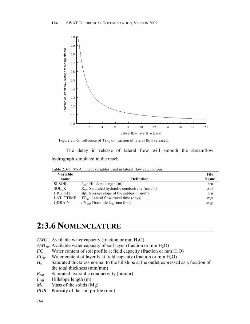
164 SWAT THEORETICAL DOCUMENTATION, VERSION 2009
164
Figure 2:3-5: Influence of TTlag on fraction of lateral flow released.
The delay in release of lateral flow will smooth the streamflow
hydrograph simulated in the reach.
Table 2:3-6: SWAT input variables used in lateral flow calculations. Variable
name
Definition File
Name SLSOIL Lhill: Hillslope length (m) .hru SOL_K Ksat: Saturated hydraulic conductivity (mm/hr) .sol HRU_SLP slp: Average slope of the subbasin (m/m) .hru LAT_TTIME TTlag: Lateral flow travel time (days) .mgt GDRAIN tilelag: Drain tile lag time (hrs) .mgt
2:3.6 NOMENCLATURE AWC Available water capacity (fraction or mm H2O) AWCly Available water capacity of soil layer (fraction or mm H2O) FC Water content of soil profile at field capacity (fraction or mm H2O) FCly Water content of layer ly at field capacity (fraction or mm H2O) Ho Saturated thickness normal to the hillslope at the outlet expressed as a fraction of
the total thickness (mm/mm) Ksat Saturated hydraulic conductivity (mm/hr) Lhill Hillslope length (m) MS Mass of the solids (Mg) POR Porosity of the soil profile (mm)

CHAPTER 2:3: EQUATIONS—SOIL WATER
165
165
Qlat Lateral flow; water discharged from the hillslope outlet (mm H2O/day) Qlatstor,i-1 Lateral flow stored or lagged from the previous day (mm H2O) Qsurf Accumulated runoff or rainfall excess (mm H2O) Rday Amount of rainfall on a given day (mm H2O) SATly Amount of water in the soil layer when completely saturated (mm H2O) SW Amount of water in soil profile (mm H2O) SWly Soil water content of layer ly (mm H2O) SWly,excess Drainable volume of water stored layer (mm H2O) TTlag Lateral flow travel time (days) TTperc Travel time for percolation (hrs) VA Volume of air (m3) VS Volume of solids (m3) VT Total soil volume (m3) VW Volume of water (m3) WP Water content at wilting point (fraction or mm H2O) WPly Water content of the soil layer at wilting point (fraction or mm H2O)
coefcrk Adjustment coefficient for crack flow
crk Total crack volume for the soil profile on a given day (mm) crkly Crack volume for the soil layer on a given day expressed as a depth (mm) crkly,d-1 Crack volume for the soil layer on the previous day (mm) crkly,i Initial crack volume calculated for the soil layer on a given day expressed as a
depth (mm) crkmax Potential crack volume for the soil profile expressed as a fraction of the total
volume crkmax,ly Maximum crack volume possible for the soil layer (mm) depthdiff Distance from the bottom of the soil profile to the impervious layer (m) depthimp Depth to the impervious layer (mm) depthly Depth of the soil layer (mm) hwtbl Water table height (m) mc Percent clay content slp Average slope of the subbasin (% or m/m) tilelag Drain tile lag time (hrs). vlat Velocity of flow at the hillslope outlet (mm∙h-1) wcrk,btm Amount of water flow past the lower boundary of the soil profile due to bypass
flow (mm H2O) winf Amount of water entering the soil profile on a given day (mm H2O) wperc,ly Amount of water percolating to the underlying soil layer on a given day (mm
H2O) zl,ly Depth from the surface to the bottom of the soil layer (mm)
hill Slope of the hillslope segment (degrees) t Length of the time step (hrs)
crk Lag factor for crack development during drying b Bulk density (Mg m-3) s Particle density (Mg m-3)

166 SWAT THEORETICAL DOCUMENTATION, VERSION 2009
166
air Air-filled porosity expressed as a fraction d Drainable porosity of the soil (mm/mm) fc Porosity of the soil layer filled with water when the layer is at field capacity water
content (mm/mm) soil Porosity of the soil (mm/mm)
2:3.7 REFERENCES
Bouma, J. and J. Loveday. 1988. Chapter 5: Characterizing soil water regimes in
swelling clay soils. p. 83-96. In L.P. Wilding and R. Puentes (ed).
Vertisols: their distribution, properties, classification and management.
Texas A&M University Printing Center, College Station, TX.
Bronswijk, J.J.B. 1989. Prediction of actual cracking and subsidence in clay soils.
Soil Science 148:87-93.
Bronswijk, J.J.B. 1990. Shrinkage geometry of a heavy clay soil at various
stresses. Soil Science Soc. Am. J. 54:1500-1502.
Dudal, R. and H. Eswaran. 1988. Chapter 1: Distribution, properties and
classification of vertisols. p. 1-22. In L.P. Wilding and R. Puentes (ed).
Vertisols: their distribution, properties, classification and management.
Texas A&M University Printing Center, College Station, TX.
Koorevaar, P., G. Menelik, and C. Dirksen. 1983. Elements of Soil Physics.
Elsevier, Amsterdam.
Mitchell, A.R. 1992. Shrinkage terminology: escape from ‘normalcy’. Soil. Sci.
Soc. Am. J. 56:993-994.
Sloan, P.G. and I.D. Moore. 1984. Modeling subsurface stormflow on steeply
sloping forested watersheds. Water Resources Research. 20(12): 1815-
1822.
Sloan, P.G., I.D. Morre, G.B. Coltharp, and J.D. Eigel. 1983. Modeling surface
and subsurface stormflow on steeply-sloping forested watersheds. Water
Resources Inst. Report 142. Univ. Kentucky, Lexington.

CHAPTER 2:3: EQUATIONS—SOIL WATER
167
167

168
SECTION 2 CHAPTER 4
EQUATIONS:
GROUNDWATER
Groundwater is water in the saturated zone of earth materials under
pressure greater than atmospheric, i.e. positive pressure. Remember that in the
soil profile water is held at a negative pressure due to the attraction between
negatively charged clay particles and water. The groundwater table is the depth at
which the pressure between water and the surrounding soil matrix is equal to
atmospheric pressure. Water enters groundwater storage primarily by
infiltration/percolation, although recharge by seepage from surface water bodies
may occur. Water leaves groundwater storage primarily by discharge into rivers
or lakes, but it is also possible for water to move upward from the water table into
the capillary fringe, a zone above the groundwater table that is saturated.

CHAPTER 2:4: EQUATIONS—GROUNDWATER
169
169
2:4.1 GROUNDWATER SYSTEMS Within the saturated zone of groundwater, regions of high conductivity
and low conductivity will be found. The regions of high conductivity are made up
of coarse-grained particles with a large percentage of macropores that allow water
to move easily. The regions of low conductivity are made up of fine-grained
particles with a large percentage of mesopores and micropores that restrict the rate
of water movement.
An aquifer is “a geologic unit that can store enough water and transmit it
at a rate fast enough to be hydrologically significant” (Dingman, 1994). An
unconfined aquifer is an aquifer whose upper boundary is the water table. A
confined aquifer is an aquifer bounded above and below by geologic formations
whose hydraulic conductivity is significantly lower than that of the aquifer. Figure
2:4-1 illustrates the two types of aquifers. Figure 2:4-1: Unconfined and confined aquifers (After Dingman, 1994).
Recharge to unconfined aquifers occurs via percolation to the water table
from a significant portion of the land surface. In contrast, recharge to confined
aquifers by percolation from the surface occurs only at the upstream end of the
confined aquifer, where the geologic formation containing the aquifer is exposed
at the earth‟s surface, flow is not confined, and a water table is present.

170 SWAT THEORETICAL DOCUMENTATION, VERSION 2009
170
Topography exerts an important influence on groundwater flow. The flow
of groundwater in an idealized hilly upland area is depicted in Figure 2:4-2. The
landscape can be divided into areas of recharge and areas of discharge. A recharge
area is defined as a portion of a drainage basin where ground water flow is
directed away from the water table. A discharge area is defined as a portion of the
drainage basin where ground water flow is directed toward the water table. The
water table is at or near the surface in discharge areas and surface water bodies
are normally located in discharge areas.
Figure 2:4-2: Groundwater flow net in an idealized hilly region with homogenous permeable material resting on an impermeable base (After Hubbert, 1940)
Streams may be categorized by their relationship to the groundwater
system. A stream located in a discharge area that receives groundwater flow is a
gaining or effluent stream (Figure 2:4-3a). This type of stream is characterized by
an increase in discharge downstream. A stream located in a recharge area is a
losing or influent stream. This type of stream is characterized by a decrease in
discharge downstream. A losing stream may be connected to (Figure 2:4-3b) or
perched above (Figure 2:4-3c) the groundwater flow area. A stream that
simultaneously receives and loses groundwater is a flow-through stream (Figure
2:4-3d).

CHAPTER 2:4: EQUATIONS—GROUNDWATER
171
171
Figure 2:4-3: Stream-groundwater relationships: a) gaining stream receiving water from groundwater flow; b) losing stream connected to groundwater system; c) losing stream perched above groundwater system; and d) flow-through stream (After Dingman, 1994).
SWAT simulates two aquifers in each subbasin. The shallow aquifer is an
unconfined aquifer that contributes to flow in the main channel or reach of the
subbasin. The deep aquifer is a confined aquifer. Water that enters the deep
aquifer is assumed to contribute to streamflow somewhere outside of the
watershed (Arnold et al., 1993).
2:4.2 SHALLOW AQUIFER
The water balance for the shallow aquifer is:
shpumprevapgwshrchrgishish wwQwaqaq ,,1,, 2:4.2.1
where aqsh,i is the amount of water stored in the shallow aquifer on day i (mm
H2O), aqsh,i-1 is the amount of water stored in the shallow aquifer on day i-1 (mm
H2O), wrchrg,sh is the amount of recharge entering the shallow aquifer on day i (mm
H2O), Qgw is the groundwater flow, or base flow, into the main channel on day i
(mm H2O), wrevap is the amount of water moving into the soil zone in response to
water deficiencies on day i (mm H2O), and wpump,sh is the amount of water
removed from the shallow aquifer by pumping on day i (mm H2O).

172 SWAT THEORETICAL DOCUMENTATION, VERSION 2009
172
2:4.2.1 RECHARGE Water that moves past the lowest depth of the soil profile by percolation or
bypass flow enters and flows through the vadose zone before becoming shallow
and/or deep aquifer recharge. The lag between the time that water exits the soil
profile and enters the shallow aquifer will depend on the depth to the water table
and the hydraulic properties of the geologic formations in the vadose and
groundwater zones.
An exponential decay weighting function proposed by Venetis (1969) and
used by Sangrey et al. (1984) in a precipitation/groundwater response model is
utilized in SWAT to account for the time delay in aquifer recharge once the water
exits the soil profile. The delay function accommodates situations where the
recharge from the soil zone to the aquifer is not instantaneous, i.e. 1 day or less.
The recharge to both aquifers on a given day is calculated:
1,, 1exp1exp1 irchrggwseepgwirchrg www 2:4.2.2
where wrchrg,i is the amount of recharge entering the aquifers on day i (mm H2O),
gw is the delay time or drainage time of the overlying geologic formations (days),
wseep is the total amount of water exiting the bottom of the soil profile on day i
(mm H2O), and wrchrg,i-1 is the amount of recharge entering the aquifers on day i-1
(mm H2O). The total amount of water exiting the bottom of the soil profile on day
i is calculated:
btmcrknlypercseep www ,, 2:4.2.3
where wseep is the total amount of water exiting the bottom of the soil profile on
day i (mm H2O), wperc,ly=n is the amount of water percolating out of the lowest
layer, n, in the soil profile on day i (mm H2O), and wcrk,btm is the amount of water
flow past the lower boundary of the soil profile due to bypass flow on day i (mm
H2O).
The delay time, gw, cannot be directly measured. It can be estimated by
simulating aquifer recharge using different values for gw and comparing the
simulated variations in water table level with observed values. Johnson (1977)
developed a simple program to iteratively test and statistically evaluate different

CHAPTER 2:4: EQUATIONS—GROUNDWATER
173
173
delay times for a watershed. Sangrey et al. (1984) noted that monitoring wells in
the same area had similar values for gw, so once a delay time value for a
geomorphic area is defined, similar delay times can be used in adjoining
watersheds within the same geomorphic province.
2:4.2.2 PARTITIONING OF RECHARGE BETWEEN SHALLOW AND DEEP AQUIFER
A fraction of the total daily recharge can be routed to the deep aquifer.
The amount of water than will be diverted from the shallow aquifer due to
percolation to the deep aquifer on a given day is:
rchrgdeepdeep ww 2:4.2.4
where wdeep is the amount of water moving into the deep aquifer on day i (mm
H2O), deep is the aquifer percolation coefficient, and wrchrg is the amount of
recharge entering both aquifers on day i (mm H2O). The amount of recharge to
the shallow aquifer is:
deeprchrgshrchrg www , 2:4.2.5
where wrchrg,sh is the amount of recharge entering the shallow aquifer on day i
(mm H2O).
2:4.2.3 GROUNDWATER/BASE FLOW The shallow aquifer contributes base flow to the main channel or reach
within the subbasin. Base flow is allowed to enter the reach only if the amount of
water stored in the shallow aquifer exceeds a threshold value specified by the
user, aqshthr,q.
The steady-state response of groundwater flow to recharge is (Hooghoudt,
1940):
wtbl
gw
satgw h
L
KQ
2
8000 2:4.2.6
where Qgw is the groundwater flow, or base flow, into the main channel on day i
(mm H2O), Ksat is the hydraulic conductivity of the aquifer (mm/day), Lgw is the
distance from the ridge or subbasin divide for the groundwater system to the main
channel (m), and hwtbl is the water table height (m).

174 SWAT THEORETICAL DOCUMENTATION, VERSION 2009
174
Water table fluctuations due to non-steady-state response of groundwater
flow to periodic recharge is calculated (Smedema and Rycroft, 1983):
800, gwshrchrgwtbl
Qw
dt
dh 2:4.2.7
where dt
dhwtbl is the change in water table height with time (mm/day), wrchrg,sh is
the amount of recharge entering the shallow aquifer on day i (mm H2O), Qgw is
the groundwater flow into the main channel on day i (mm H2O), and is the
specific yield of the shallow aquifer (m/m).
Assuming that variation in groundwater flow is linearly related to the rate
of change in water table height, equations 2:4.2.7 and 2:4.2.6 can be combined to
obtain:
gwshrchrggwgwshrchrg
gw
satgwQwQw
L
K
dt
dQ
,,210
2:4.2.8
where Qgw is the groundwater flow into the main channel on day i (mm H2O), Ksat
is the hydraulic conductivity of the aquifer (mm/day), is the specific yield of the
shallow aquifer (m/m), Lgw is the distance from the ridge or subbasin divide for
the groundwater system to the main channel (m), wrchrg,sh is the amount of
recharge entering the shallow aquifer on day i (mm H2O) and gw is the baseflow
recession constant or constant of proportionality. Integration of equation 2:4.2.8
and rearranging to solve for Qgw yields:
twtQQ gwshrchrggwigwigw exp1exp ,1,,
if qshthrsh aqaq , 2:4.2.9
0, igwQ if qshthrsh aqaq , 2:4.2.10
where Qgw,i is the groundwater flow into the main channel on day i (mm H2O),
Qgw,i-1 is the groundwater flow into the main channel on day i-1 (mm H2O), gw is
the baseflow recession constant, t is the time step (1 day), wrchrg,sh is the amount
of recharge entering the shallow aquifer on day i (mm H2O), aqsh is the amount of
water stored in the shallow aquifer at the beginning of day i (mm H2O) and

CHAPTER 2:4: EQUATIONS—GROUNDWATER
175
175
aqshthr,q is the threshold water level in the shallow aquifer for groundwater
contribution to the main channel to occur (mm H2O).
The baseflow recession constant, gw, is a direct index of groundwater
flow response to changes in recharge (Smedema and Rycroft, 1983). Values vary
from 0.1-0.3 for land with slow response to recharge to 0.9-1.0 for land with a
rapid response. Although the baseflow recession constant may be calculated, the
best estimates are obtained by analyzing measured streamflow during periods of
no recharge in the watershed.
When the shallow aquifer receives no recharge, equation 2:4.2.9 simplifies
to:
tQQ gwgwgw exp0, if qshthrsh aqaq , 2:4.2.11
0, igwQ if qshthrsh aqaq , 2:4.2.12
where Qgw is the groundwater flow into the main channel at time t (mm H2O),
Qgw,0 is the groundwater flow into the main channel at the beginning of the
recession (time t=0) (mm H2O), gw is the baseflow recession constant, and t is
the time lapsed since the beginning of the recession (days), aqsh is the amount of
water stored in the shallow aquifer at the beginning of day i (mm H2O) and
aqshthr,q is the threshold water level in the shallow aquifer for groundwater
contribution to the main channel to occur (mm H2O). The baseflow recession
constant is measured by rearranging equation 2:4.2.11.
0,
,ln1
gw
Ngw
gwQ
Q
N 2:4.2.13
where gw is the baseflow recession constant, N is the time lapsed since the start
of the recession (days), Qgw,N is the groundwater flow on day N (mm H2O), Qgw,0
is the groundwater flow at the start of the recession (mm H2O).
It is common to find the baseflow days reported for a stream gage or
watershed. This is the number of days for base flow recession to decline through
one log cycle. When baseflow days are used, equation 2:4.2.13 can be further
simplified:

176 SWAT THEORETICAL DOCUMENTATION, VERSION 2009
176
BFDBFDQ
Q
N gw
Ngw
gw
3.210ln1ln1
0,
,
2:4.2.14
where gw is the baseflow recession constant, and BFD is the number of baseflow
days for the watershed.
2:4.2.4 REVAP Water may move from the shallow aquifer into the overlying unsaturated
zone. In periods when the material overlying the aquifer is dry, water in the
capillary fringe that separates the saturated and unsaturated zones will evaporate
and diffuse upward. As water is removed from the capillary fringe by evaporation,
it is replaced by water from the underlying aquifer. Water may also be removed
from the aquifer by deep-rooted plants which are able to uptake water directly
from the aquifer.
SWAT models the movement of water into overlying unsaturated layers as
a function of water demand for evapotranspiration. To avoid confusion with soil
evaporation and transpiration, this process has been termed „revap‟. This process
is significant in watersheds where the saturated zone is not very far below the
surface or where deep-rooted plants are growing. Because the type of plant cover
will affect the importance of revap in the water balance, the parameters governing
revap are usually varied by land use. Revap is allowed to occur only if the amount
of water stored in the shallow aquifer exceeds a threshold value specified by the
user, aqshthr,rvp.
The maximum amount of water than will be removed from the aquifer via
„revap‟ on a given day is:
orevmxrevap Ew , 2:4.2.15
where wrevap,mx is the maximum amount of water moving into the soil zone in
response to water deficiencies (mm H2O), rev is the revap coefficient, and Eo is
the potential evapotranspiration for the day (mm H2O). The actual amount of
revap that will occur on a given day is calculated:
0revapw if rvpshthrsh aqaq , 2:4.2.16
rvpshthrmxrevaprevap aqww ,, if mxrevaprvpshthrshrvpshthr waqaqaq ,,, 2:4.2.17

CHAPTER 2:4: EQUATIONS—GROUNDWATER
177
177
mxrevaprevap ww , if mxrevaprvpshthrsh waqaq ,, 2:4.2.18
where wrevap is the actual amount of water moving into the soil zone in response to
water deficiencies (mm H2O), wrevap,mx is the maximum amount of water moving
into the soil zone in response to water deficiencies (mm H2O), aqsh is the amount
of water stored in the shallow aquifer at the beginning of day i (mm H2O) and
aqshthr,rvp is the threshold water level in the shallow aquifer for revap to occur (mm
H2O).
2:4.2.5 PUMPING If the shallow aquifer is specified as the source of irrigation water or water
removed for use outside the watershed, the model will allow an amount of water
up to the total volume of the shallow aquifer to be removed on any given day.
Detailed information on water management may be found in Chapter 6:2.
2:4.2.6 GROUNDWATER HEIGHT Although SWAT does not currently print groundwater height in the output
files, the water table height is updated daily by the model. Groundwater height is
related to groundwater flow by equation 2:4.2.6.
wtblgwwtbl
gw
satwtbl
gw
satgw hh
L
Kh
L
KQ
8001010
8000800022 2:4.2.19
where Qgw is the groundwater flow into the main channel on day i (mm H2O), Ksat
is the hydraulic conductivity of the aquifer (mm/day), Lgw is the distance from the
ridge or subbasin divide for the groundwater system to the main channel (m), hwtbl
is the water table height (m), is the specific yield of the shallow aquifer (m/m),
and gw is the baseflow recession constant. Substituting this definition for Qgw
into equation 2:4.2.9 gives
gw
gwrchrg
gwiwtbliwtbl
twthh
800
exp1exp1,, 2:4.2.20
where hwtbl,i is the water table height on day i (m), hwtbl,i-1 is the water table height
on day i-1 (m), gw is the baseflow recession constant, t is the time step (1 day),
wrchrg is the amount of recharge entering the aquifer on day i (mm H2O), and is
the specific yield of the shallow aquifer (m/m).
178 SWAT THEORETICAL DOCUMENTATION, VERSION 2009
178
Table 2:4-1: SWAT input variables used in shallow aquifer calculations. Variable
name
Definition File
Name GW_DELAY gw: Delay time for aquifer recharge (days) .gw GWQMN aqshthr,q: Threshold water level in shallow aquifer for base flow (mm
H2O) .gw
ALPHA_BF gw: Baseflow recession constant .gw REVAPMN aqshthr,rvp: Threshold water level in shallow aquifer for revap (mm H2O) .gw GW_REVAP rev: Revap coefficient .gw RCHRG_DP deep: Aquifer percolation coefficient .gw GW_SPYLD : Specific yield of the shallow aquifer (m/m) .gw
2:4.3 DEEP AQUIFER The water balance for the deep aquifer is:
dppumpdeepidpidp wwaqaq ,1,, 2:4.3.1
where aqdp,i is the amount of water stored in the deep aquifer on day i (mm H2O),
aqdp,i-1 is the amount of water stored in the deep aquifer on day i-1 (mm H2O),
wdeep is the amount of water percolating from the shallow aquifer into the deep
aquifer on day i (mm H2O), and wpump,dp is the amount of water removed from the
deep aquifer by pumping on day i (mm H2O). The amount of water percolating
into the deep aquifer is calculated with the equations reviewed in section 2:4.2.4.
If the deep aquifer is specified as the source of irrigation water or water removed
for use outside the watershed, the model will allow an amount of water up to the
total volume of the deep aquifer to be removed on any given day.
Water entering the deep aquifer is not considered in future water budget
calculations and can be considered to be lost from the system.

CHAPTER 2:4: EQUATIONS—GROUNDWATER
179
179
2:4.4 NOMENCLATURE BFD Number of baseflow days for the watershed
Eo Potential evapotranspiration (mm d-1) Ksat Hydraulic conductivity of the aquifer (mm/day) Lgw Distance from the ridge or subbasin divide for the groundwater system to the
main channel (m) N Time lapsed since the start of the recession (days) Qgw Groundwater flow, or base flow, into the main channel (mm H2O) Qgw,0 Groundwater flow at the start of the recession (mm H2O) Qgw,N Groundwater flow on day N (mm H2O)
aqdp Amount of water stored in the deep aquifer (mm H2O) aqsh Amount of water stored in the shallow aquifer (mm H2O) aqshthr,q Threshold water level in shallow aquifer for base flow (mm H2O) aqshthr,rvp Threshold water level in shallow aquifer for revap or percolation to deep aquifer
(mm H2O) hwtbl Water table height (m) wcrk,btm Amount of water flow past the lower boundary of the soil profile due to bypass
flow (mm H2O) wdeep Amount of water percolating from the shallow aquifer into the deep aquifer (mm
H2O) wpump,dp Amount of water removed from the deep aquifer by pumping (mm H2O) wpump,sh Amount of water removed from the shallow aquifer by pumping (mm H2O) wrchrg Amount of water entering the aquifer via recharge (mm H2O) wrchrg,sh Amount of water entering the shallow aquifer via recharge (mm H2O) wrevap Amount of water moving into the soil zone in response to water deficiencies (mm
H2O) wrevap,mx Maximum amount of water moving into the soil zone in response to water
deficiencies on day i (mm H2O) wseep Total amount of water exiting the bottom of the soil profile (mm H2O)
gw Baseflow recession constant deep Aquifer percolation coefficient rev Revap coefficient gw Delay time or drainage time for aquifer recharge (days) Specific yield of the shallow aquifer (m/m)

180 SWAT THEORETICAL DOCUMENTATION, VERSION 2009
180
2:4.5 REFERENCES
Arnold, J.G., P.M. Allen, and G. Bernhardt. 1993. A comprehensive surface-
groundwater flow model. Journal of Hydrology 142: 47-69.
Dingman, S.L. 1994. Physical hydrology. Prentice-Hall, Inc., Englewood Cliffs,
NJ.
Hooghoudt, S.B. 1940. Bijdrage tot de kennis van enige natuurkundige
grootheden van de grond. Versl. Landbouwkd. Onderz. 46: 515-707.
Hubbert, M.K. 1940. The theory of groundwater motion. Journal of Geology
48: 785-944.
Johnson, K.H. 1977. A predictive method for ground water levels. Master‟s
Thesis, Cornell University, Ithica, N.Y.
Sangrey, D.A., K.O. Harrop-Williams, and J.A. Klaiber. 1984. Predicting ground-
water response to precipitation. ASCE J. Geotech. Eng. 110(7): 957-975.
Smedema, L.K. and D.W. Rycroft. 1983. Land drainage—planning and design of
agricultural drainage systems, Cornell University Press, Ithica, N.Y.
Venetis, C. 1969. A study of the recession of unconfined aquifers. Bull. Int.
Assoc. Sci. Hydrol. 14(4): 119-125.

CHAPTER 2:4: EQUATIONS—GROUNDWATER
181
181

NUTRIENTS & PESTICIDES
The fate and transport of nutrients and pesticides
in a watershed depend on the transformations the
compounds undergo in the soil environment. SWAT
models the complete nutrient cycle for nitrogen and
phosphorus as well as the degradation of any pesticides
applied in an HRU.
The following three chapters review the
methodology used by SWAT to simulate nutrient and
pesticide processes in the soil.

182
SECTION 3 CHAPTER 1
EQUATIONS:
NITROGEN
The complexity of the nitrogen cycle and nitrogen’s importance in plant
growth have made this element the subject of much research. The nitrogen cycle
is a dynamic system that includes the water, atmosphere and soil. Plants require
nitrogen more than any other essential element, excluding carbon, oxygen and
hydrogen. Nitrogen is modeled by SWAT in the soil profile and in the shallow
aquifer.

CHAPTER 3:1: EQUATIONS—NITROGEN
183
183
3:1.1 NITROGEN CYCLE IN THE SOIL
The three major forms of nitrogen in mineral soils are organic nitrogen
associated with humus, mineral forms of nitrogen held by soil colloids, and
mineral forms of nitrogen in solution. Nitrogen may be added to the soil by
fertilizer, manure or residue application, fixation by symbiotic or nonsymbiotic
bacteria, and rain. Nitrogen is removed from the soil by plant uptake, leaching,
volatilization, denitrification and erosion. Figure 3:1-1 shows the major
components of the nitrogen cycle.
Figure 3:1-1: The nitrogen cycle
Nitrogen is considered to be an extremely reactive element. The highly
reactive nature of nitrogen results from its ability to exist in a number of valance
states. The valence state or oxidation state describes the number of electrons
orbiting the nucleus of the nitrogen atom relative to the number present in an

184 SWAT THEORETICAL DOCUMENTATION, VERSION 2009
184
electronically neutral atom. The valence state will be positive as the atom looses
electrons and will be negative as the atom gains electrons. Examples of nitrogen
in different valence states are:
most oxidized +5 -3NO nitrate
+4 2NO nitrogen dioxide +3 -
2NO nitrite +2 NO nitrogen monoxide (gas) +1 ON2 nitrous oxide (laughing gas) 0 2N N2 gas or elemental N -1 OHNH4 hydroxylamine -2 42HN hydrozine most reduced -3 NH3 or
4NH ammonia gas or ammonium
The ability of nitrogen to vary its valence state makes it a highly mobile element.
Predicting the movement of nitrogen between the different pools in the soil is
critical to the successful management of this element in the environment.
SWAT monitors five different pools of nitrogen in the soil (Figure 3:1-2).
Two pools are inorganic forms of nitrogen, NH4+ and -
3NO , while the other three
pools are organic forms of nitrogen. Fresh organic N is associated with crop
residue and microbial biomass while the active and stable organic N pools are
associated with the soil humus. The organic nitrogen associated with humus is
partitioned into two pools to account for the variation in availability of humic
substances to mineralization.
Figure 3:1-2: SWAT soil nitrogen pools and processes that move nitrogen in and out of pools.

CHAPTER 3:1: EQUATIONS—NITROGEN
185
185
3:1.1.1 INITIALIZATION OF SOIL NITROGEN LEVELS Users may define the amount of nitrate and organic nitrogen contained in
humic substances for all soil layers at the beginning of the simulation. If the user
does not specify initial nitrogen concentrations, SWAT will initialize levels of
nitrogen in the different pools.
Initial nitrate levels in the soil are varied by depth using the relationship:
1000exp7,
zNO3 zconc
3:1.1.1
where NO3conc,z is the concentration of nitrate in the soil at depth z (mg/kg or
ppm), and z is the depth from the soil surface (mm). The nitrate concentration
with depth calculated from equation 3:1.1.1 is displayed in Figure 3:1-3. The
nitrate concentration for a layer is calculated by solving equation 3:1.1.1 for the
horizon’s lower boundary depth.
Figure 3:1-3: Nitrate concentration with depth.
Organic nitrogen levels are assigned assuming that the C:N ratio for humic
materials is 14:1. The concentration of humic organic nitrogen in a soil layer is
calculated:
14104
,ly
lyhum
orgCorgN 3:1.1.2

186 SWAT THEORETICAL DOCUMENTATION, VERSION 2009
186
where orgNhum,ly is the concentration of humic organic nitrogen in the layer
(mg/kg or ppm), and orgCly is the amount of organic carbon in the layer (%). The
humic organic N is partitioned between the active and stable pools using the
following equations:
actNlyhumlyact frorgNorgN ,, 3:1.1.3
actNlyhumlysta frorgNorgN 1,, 3:1.1.4
where orgNact,ly is the concentration of nitrogen in the active organic pool
(mg/kg), orgNhum,ly is the concentration of humic organic nitrogen in the layer
(mg/kg), fractN is the fraction of humic nitrogen in the active pool, and orgNsta,ly is
the concentration of nitrogen in the stable organic pool (mg/kg). The fraction of
humic nitrogen in the active pool, fractN, is set to 0.02.
Nitrogen in the fresh organic pool is set to zero in all layers except the top
10 mm of soil. In the top 10 mm, the fresh organic nitrogen pool is set to 0.15%
of the initial amount of residue on the soil surface.
surfsurffrsh rsdorgN 0015.0, 3:1.1.5
where orgNfrsh,surf is the nitrogen in the fresh organic pool in the top 10 mm (kg
N/ha), and rsdsurf is material in the residue pool for the top 10 mm of soil (kg/ha).
The ammonium pool for soil nitrogen, NH4ly, is initialized to 0 ppm.
While SWAT allows nutrient levels to be input as concentrations, it
performs all calculations on a mass basis. To convert a concentration to a mass,
the concentration is multiplied by the bulk density and depth of the layer and
divided by 100:
ha
N kg100
lybN depthconc
3:1.1.6
where concN is the concentration of nitrogen in a layer (mg/kg or ppm), b is the
bulk density of the layer (Mg/m3), and depthly is the depth of the layer (mm).

CHAPTER 3:1: EQUATIONS—NITROGEN
187
187
Table 3:1-1: SWAT input variables that pertain to nitrogen pools.
Variable Name
Definition Input File
SOL_NO3 NO3conc,ly: Initial NO3 concentration in soil layer (mg/kg or ppm) .chm SOL_ORGN orgNhum,ly: Initial humic organic nitrogen in soil layer (mg/kg or
ppm) .chm
RSDIN rsdsurf: Material in the residue pool for the top 10mm of soil (kg ha-1) .hru SOL_BD b: Bulk density of the layer (Mg/m3) .sol SOL_CBN orgCly: Amount of organic carbon in the layer (%) .sol
3:1.2 MINERALIZATION & DECOMPOSITION / IMMOBILIZATION
Decomposition is the breakdown of fresh organic residue into simpler
organic components. Mineralization is the microbial conversion of organic, plant-
unavailable nitrogen to inorganic, plant-available nitrogen. Immobilization is the
microbial conversion of plant-available inorganic soil nitrogen to plant-
unavailable organic nitrogen.
Bacteria decompose organic material to obtain energy for growth
processes. Plant residue is broken down into glucose which is then converted to
energy:
OH66COOOHC 22releasedenergy
26126
The energy released by the conversion of glucose to carbon dioxide and water is
used for various cell processes, including protein synthesis. Protein synthesis
requires nitrogen. If the residue from which the glucose is obtained contains
enough nitrogen, the bacteria will use nitrogen from the organic material to meet
the demand for protein synthesis. If the nitrogen content of the residue is too low
to meet the bacterial demand for nitrogen, the bacteria will use NH4+ and -
3NO
from the soil solution to meet its needs. If the nitrogen content of the residue
exceeds the bacterial demand for nitrogen, the bacterial will release the excess
nitrogen into soil solution as NH4+. A general relationship between C:N ratio and
mineralization/immobilization is:
C:N > 30:1 immobilization occurs, a net decrease in soil NH4+ and -
3NO
20:1 C:N 30:1 expect no net change; immobilization and mineralization processes are at equilibrium

188 SWAT THEORETICAL DOCUMENTATION, VERSION 2009
188
C:N < 20:1 mineralization occurs, a net gain in soil NH4+ and -
3NO
The nitrogen mineralization algorithms in SWAT are net mineralization
algorithms which incorporate immobilization into the equations. The algorithms
were adapted from the PAPRAN mineralization model (Seligman and van
Keulen, 1981). Two sources are considered for mineralization: the fresh organic
N pool associated with crop residue and microbial biomass and the active organic
N pool associated with soil humus. Mineralization and decomposition are allowed
to occur only if the temperature of the soil layer is above 0C.
Mineralization and decomposition are dependent on water availability and
temperature. Two factors are used in the mineralization and decomposition
equations to account for the impact of temperature and water on these processes.
The nutrient cycling temperature factor is calculated:
1.0
312.093.9exp9.0
,,
,,
lysoillysoil
lysoil
lytmpTT
T 3:1.2.1
where tmp,ly is the nutrient cycling temperature factor for layer ly, and Tsoil,ly is the
temperature of layer ly (C). The nutrient cycling temperature factor is never
allowed to fall below 0.1.
The nutrient cycling water factor is calculated:
ly
ly
lyswFC
SW, 3:1.2.2
where sw,ly is the nutrient cycling water factor for layer ly, SWly is the water
content of layer ly on a given day (mm H2O), and FCly is the water content of
layer ly at field capacity (mm H2O). The nutrient cycling water factor is never
allowed to fall below 0.05.
3:1.2.1 HUMUS MINERALIZATION Nitrogen is allowed to move between the active and stable organic pools
in the humus fraction. The amount of nitrogen transferred from one pool to the
other is calculated:
lysta
actN
lyacttrnslytrns orgNfr
orgNN ,,, 11
3:1.2.3

CHAPTER 3:1: EQUATIONS—NITROGEN
189
189
Ntrns,ly is the amount of nitrogen transferred between the active and stable organic
pools (kg N/ha), trns is the rate constant (110-5), orgNact,ly is the amount of
nitrogen in the active organic pool (kg N/ha), fractN is the fraction of humic
nitrogen in the active pool (0.02), and orgNsta,ly is the amount of nitrogen in the
stable organic pool (kg N/ha). When Ntrns,ly is positive, nitrogen is moving from
the active organic pool to the stable organic pool. When Ntrns,ly is negative,
nitrogen is moving from the stable organic pool to the active organic pool.
Mineralization from the humus active organic N pool is calculated:
lyactlyswlytmpminmina,ly orgNN ,21
,, 3:1.2.4
where Nmina,ly is the nitrogen mineralized from the humus active organic N pool
(kg N/ha), min is the rate coefficient for mineralization of the humus active
organic nutrients, tmp,ly is the nutrient cycling temperature factor for layer ly, sw,ly
is the nutrient cycling water factor for layer ly, orgNact,ly is the amount of nitrogen
in the active organic pool (kg N/ha).
Nitrogen mineralized from the humus active organic pool is added to the
nitrate pool in the layer.
3:1.2.2 RESIDUE DECOMPOSITION & MINERALIZATION Decomposition and mineralization of the fresh organic nitrogen pool is
allowed only in the first soil layer. Decomposition and mineralization are
controlled by a decay rate constant that is updated daily. The decay rate constant
is calculated as a function of the C:N ratio and C:P ratio of the residue,
temperature and soil water content.
The C:N ratio of the residue is calculated:
lylyfrsh
ly
NCNO3orgN
rsd
,:
58.0 3:1.2.5
where C:N is the C:N ratio of the residue in the soil layer, rsdly is the residue in
layer ly (kg/ha), 0.58 is the fraction of residue that is carbon, orgNfrsh,ly is the
nitrogen in the fresh organic pool in layer ly (kg N/ha), and NO3ly is the amount
of nitrate in layer ly (kg N/ha).
The C:P ratio of the residue is calculated:

190 SWAT THEORETICAL DOCUMENTATION, VERSION 2009
190
lysolutionlyfrsh
ly
PCPorgP
rsd
,,:
58.0
3:1.2.6
where C:P is the C:P ratio of the residue in the soil layer, rsdly is the residue in
layer ly (kg/ha), 0.58 is the fraction of residue that is carbon, orgPfrsh,ly is the
phosphorus in the fresh organic pool in layer ly (kg P/ha), and Psolution,ly is the
amount of phosphorus in solution in layer ly (kg P/ha).
The decay rate constant defines the fraction of residue that is decomposed.
The decay rate constant is calculated:
21,,,, lyswlytmplyntrrsdlyntr 3:1.2.7
where ntr,ly is the residue decay rate constant, rsd is the rate coefficient for
mineralization of the residue fresh organic nutrients, ntr,ly is the nutrient cycling
residue composition factor for layer ly, tmp,ly is the nutrient cycling temperature
factor for layer ly, and sw,ly is the nutrient cycling water factor for layer ly.
The nutrient cycling residue composition factor is calculated:
0.1
200200693.0exp
2525693.0exp
min :
:
,PC
NC
lyntr
3:1.2.8
where ntr,ly is the nutrient cycling residue composition factor for layer ly, C:N is
the C:N ratio on the residue in the soil layer, and C:P is the C:P ratio on the
residue in the soil layer.
Mineralization from the residue fresh organic N pool is then calculated:
lyfrshlyntrminf,ly orgNN ,,8.0 3:1.2.9
where Nminf,ly is the nitrogen mineralized from the fresh organic N pool (kg N/ha),
ntr,ly is the residue decay rate constant, and orgNfrsh,ly is the nitrogen in the fresh
organic pool in layer ly (kg N/ha). Nitrogen mineralized from the fresh organic
pool is added to the nitrate pool in the layer.

CHAPTER 3:1: EQUATIONS—NITROGEN
191
191
Decomposition from the residue fresh organic N pool is calculated:
lyfrshlyntrdec,ly orgNN ,,2.0 3:1.2.9
where Ndec,ly is the nitrogen decomposed from the fresh organic N pool (kg N/ha),
ntr,ly is the residue decay rate constant, and orgNfrsh,ly is the nitrogen in the fresh
organic pool in layer ly (kg N/ha). Nitrogen decomposed from the fresh organic
pool is added to the humus active organic pool in the layer.
Table 3:1-2: SWAT input variables that pertain to mineralization.
Variable Name
Definition Input File
CMN min: Rate coefficient for mineralization of the humus active organic nutrients
.bsn
RSDCO rsd: Rate coefficient for mineralization of the residue fresh organic nutrients
.bsn
RSDCO_PL rsd: Rate coefficient for mineralization of the residue fresh organic nutrients
crop.dat
3:1.3 NITRIFICATION & AMMONIA VOLATILIZATION
Nitrification is the two-step bacterial oxidation of NH4+ to -
3NO .
step 1:
4HOH2NO2O3NH2 2-2
e1224 (Nitrosomonas)
step 2: -3
-4e2
-2 2NOONO2
-
(Nitrobacter)
Ammonia volatilization is the gaseous loss of NH3 that occurs when
ammonium, NH4+, is surface applied to a calcareous soil or when urea, (NH2)2CO,
is surface applied to any soil.
NH4+ surface applied to a calcareous soil:
step 1: 232443 CaXCONHXNH2CaCO step 2: OHCO2NHCONH 22334 Urea surface applied to any soil: step 1: 324
enzyme urease222 CONHOH2CONH
step 2: OHCO2NHCONH 223324
SWAT simulates nitrification and ammonia volatilization using a
combination of the methods developed by Reddy et al. (1979) and Godwin et al.
(1984). The total amount of nitrification and ammonia volatilization is calculated,
and then partitioned between the two processes. Nitrification is a function of soil

192 SWAT THEORETICAL DOCUMENTATION, VERSION 2009
192
temperature and soil water content while ammonia volatilization is a function of
soil temperature, depth and cation exchange capacity. Four coefficients are used
in the nitrification/volatilization algorithms to account for the impact of these
parameters. Nitrification/volatilization occurs only when the temperature of the
soil layer exceeds 5C.
The nitrification/volatilization temperature factor is calculated:
105
41.0 ,,
lysoil
lytmp
T if 5, lysoilT 3:1.3.1
where tmp,ly is the nitrification/volatilization temperature factor, and Tsoil,ly is the
temperature of layer ly (C).
The nitrification soil water factor is calculated:
lyly
lyly
lyswWPFC
WPSW
25.0, if lylyly WPFCSW 75.025.0 3:1.3.2
0.1, lysw if lylyly WPFCSW 75.025.0 3:1.3.3
where sw,ly is the nitrification soil water factor, SWly is the soil water content of
layer ly on a given day (mm H2O), WPly is the amount of water held in the soil
layer at wilting point water content (mm H2O), and FCly is the amount of water
held in the soil layer at field capacity water content (mm H2O).
The volatilization depth factor is calculated:
lymidlymid
lymid
lymidzzz
z
,,
,, 0305.0706.4exp
1
3:1.3.4
where midz,ly is the volatilization depth factor, and zmid,ly is the depth from the soil
surface to the middle of the layer (mm).
SWAT does not require the user to provide information about soil cation
exchange capacity. The volatilization cation exchange factor is set to a constant
value:
15.0, lycec 3:1.3.5
The impact of environmental factors on nitrification and ammonia
volatilization in a given layer is defined by the nitrification regulator and
volatilization regulator. The nitrification regulator is calculated:

CHAPTER 3:1: EQUATIONS—NITROGEN
193
193
lyswlytmplynit ,,, 3:1.3.6
and the volatilization regulator is calculated:
lyceclymidzlytmplyvol ,,,, 3:1.3.7
where nit,ly is the nitrification regulator, vol,ly is the volatilization regulator, tmp,ly
is the nitrification/volatilization temperature factor, sw,ly is the nitrification soil
water factor, and midz,ly is the volatilization depth factor.
The total amount of ammonium lost to nitrification and volatilization is
calculated using a first-order kinetic rate equation (Reddy et al., 1979):
lyvollynitlylyvolnitNH4N ,,, exp1 3:1.3.8
where lyvolnit
N , is the amount of ammonium converted via nitrification and
volatilization in layer ly (kg N/ha), NH4ly is the amount of ammonium in layer ly
(kg N/ha), nit,ly is the nitrification regulator, and vol,ly is the volatilization
regulator.
To partition lyvolnit
N , between nitrification and volatilization, the
expression by which NH4ly is multiplied in equation 3:1.3.8, is solved using each
regulator individually to obtain a fraction of ammonium removed by each
process:
lynitlynitfr ,, exp1 3:1.3.9
lyvollyvolfr ,, exp1 3:1.3.10
where frnit,ly is the estimated fraction of nitrogen lost by nitrification, frvol,ly is the
estimated fraction of nitrogen lost by volatilization, nit,ly is the nitrification
regulator, and vol,ly is the volatilization regulator.
The amount of nitrogen removed from the ammonium pool by nitrification
is then calculated:
lyvolnit
lyvollynit
lynit
lynit Nfrfr
frN ,
,,
,,
3:1.3.11
and the amount of nitrogen removed from the ammonium pool by volatilization
is:

194 SWAT THEORETICAL DOCUMENTATION, VERSION 2009
194
lyvolnit
lyvollynit
lyvol
lyvol Nfrfr
frN ,
,,
,,
3:1.3.12
where Nnit,ly is the amount of nitrogen converted from NH4+ to -
3NO in layer ly (kg
N/ha), Nvol,ly is the amount of nitrogen converted from NH4+ to NH3 in layer ly (kg
N/ha), frnit,ly is the estimated fraction of nitrogen lost by nitrification, frvol,ly is the
estimated fraction of nitrogen lost by volatilization, and lyvolnit
N , is the amount of
ammonium converted via nitrification and volatilization in layer ly (kg N/ha)
3:1.4 DENITRIFICATION Denitrification is the bacterial reduction of nitrate, -
3NO , to N2 or N2O
gases under anaerobic (reduced) conditions. Denitrification is a function of water
content, temperature, presence of a carbon source and nitrate.
In general, when the water-filled porosity is greater than 60%
denitrification will be observed in a soil. As soil water content increases,
anaerobic conditions develop due to the fact that oxygen diffuses through water
10,000 times slower than through air. Because the rate of oxygen diffusion
through water slows as the water temperature increases, temperature will also
influence denitrification.
Cropping systems where water is ponded, such as rice, can lose a large
fraction of fertilizer by denitrification. For a regular cropping system, an
estimated 10-20% of nitrogen fertilizer may be lost to denitrification. Under a rice
cropping system, 50% of nitrogen fertilizer may be lost to denitrification. In a
flooded cropping system, the depth of water plays an important role because it
controls the amount of water oxygen has to diffuse through to reach the soil.
SWAT determines the amount of nitrate lost to denitrification with the
equation:
lylytmpdenitlylydenit orgCNO3N ,, exp1 if thrswlysw ,, 3:1.4.1
0.0, lydenitN if thrswlysw ,, 3:1.4.2
where Ndenit,ly is the amount of nitrogen lost to denitrification (kg N/ha), NO3ly is
the amount of nitrate in layer ly (kg N/ha), denit is the rate coefficient for

CHAPTER 3:1: EQUATIONS—NITROGEN
195
195
denitrification, tmp,ly is the nutrient cycling temperature factor for layer ly
calculated with equation 3:1.2.1, sw,ly is the nutrient cycling water factor for layer
ly calculated with equation 3:1.2.2, orgCly is the amount of organic carbon in the
layer (%), and sw,thr is the threshold value of nutrient cycling water factor for
denitrification to occur.
Table 3:1-3: SWAT input variables that pertain to denitrification.
Variable Name
Definition
Input File
SOL_CBN orgCly: Amount of organic carbon in the layer (%) .sol CDN denit: Rate coefficient for denitrification .bsn SDNCO sw,thr: Threshold value of nutrient cycling water factor for
denitrification to occur .bsn
3:1.5 ATMOSPHERIC DEPOSITION Atmospheric deposition occurs when airborne chemical compounds settle
onto the land or water surface. Some of the most important chemical pollutants
are those containing nitrogen or phosphorus. Nitrogen compounds can be
deposited onto water and land surfaces through both wet and dry deposition
mechanisms. Wet deposition occurs through the absorption of compounds by
precipitation as it falls carrying mainly nitrate (NO3-) and ammonium (NH4+). Dry
deposition is the direct adsorption of compounds to water or land surfaces and
involves complex interactions between airborne nitrogen compounds and plant,
water, soil, rock, or building surfaces.
The relative contribution of atmospheric deposition to total nutrient
loading is difficult to measure or indirectly assess and many deposition
mechanisms are not fully understood. Most studies and relatively extended data
sets are available on wet deposition of nitrogen, while dry deposition rates are not
well defined. Phosphorus loadings due to atmospheric deposition have not been
extensively studied and nation-wide extended data set were unavailable at the
time of data preparation for the CEAP project. While research continues in these
areas, data records generated by modeling approaches appear to be still under
scrutiny.

196 SWAT THEORETICAL DOCUMENTATION, VERSION 2009
196
A number of regional and local monitoring networks are operating in the
U.S. mainly to address information regarding regional environmental issues. For
example, the Integrated Atmospheric Deposition Network (IADN) (Galarneau et
al., 2006) that estimates deposition of toxic organic substances to the Great Lakes.
Over the CONUS (conterminous United States), the National Atmospheric
Deposition Program (NADP) National Trends Network (NTN) (NADP/NTN,
1995; NADP/NTN, 2000; Lamb and Van Bowersox, 2000) measures and
ammonium in one-week rain and snow samples at nearly 240 regionally
representative sites in the CONUS and is considered the nation’s primary source
for wet deposition data.
The U.S. EPA Clean Air Status and Trends Network (CASTNET),
developed form the National Dry Deposition Network (NDDN), operates a total
of 86 operational sites (as of December 2007) located in or near rural areas and
sensitive ecosystems collecting data on ambient levels of pollutants where urban
influences are minimal (CASTNET, 2007). As part of an interagency agreement,
the National Park Service (NPS) sponsors 27 sites which are located in national
parks and other Class-I areas designated as deserving special protection from air
pollution.
3:1.5.1 NITROGEN IN RAINFALL Lightning discharge converts atmospheric N2 to nitric acid which can then
be transferred to the soil with precipitation. The chemical steps involved are:
step 1: 2NOON yelectricit of arc22 (monoxide)
step 2: 22 NOO2NO (dioxide)
step 3: NO2HNOOH3NO 222 (nitric acid and monoxide)
More nitrogen will be added to the soil with rainfall in areas with a high amount
of lightning activity than in areas with little lightning.
The amount of nitrate added to the soil in rainfall is calculated:
dayNOrain RRNO 33 01.0 3:1.5.1
where NO3rain is nitrate added by rainfall (kg N/ha), RNO3 is the concentration of
nitrate in the rain (mg N/L), and Rday is the amount of precipitation on a given day

CHAPTER 3:1: EQUATIONS—NITROGEN
197
197
(mm H2O). The nitrogen in rainfall is added to the nitrate pool in the top 10 mm
of soil.
The amount of ammonia added to the soil in rainfall is calculated:
dayNHrain RRNH 44 01.0 3:1.5.2
where NH4rain is nitrate added by rainfall (kg N/ha), RNH4 is the concentration of
ammonia in the rain (mg N/L), and Rday is the amount of precipitation on a given
day (mm H2O). The nitrogen in rainfall is added to the ammonia pool in the top
10 mm of soil.
Table 3:1-4: SWAT input variables that pertain to nitrogen in rainfall.
Variable Name
Definition
Input File
RCN RNO3: Concentration of nitrogen in the rain (mg/L) .bsn rammo_sub Atmospheric deposition of ammonium (mg/L) values for entire
watershed .atm
Rcn_sub Atmospheric deposition of nitrate (mg/L) for entire watershed .atm
3.1.5.2 NITROGEN DRY DEPOSITION
Dry deposition of nitrate and ammonia is input to the model for each
subbasin. Average daily deposition is added to the appropriate surface soil pool.
3:1.5.3
3:1.5.4
where is the NO3 in the surface soil layer, is the ammonium in
the surface soil layer, is the daily nitrate dry deposition rate (kg/ha) and
is the daily ammonium dry deposition rate (kg/ha).
Table 3:1-5: SWAT input variables that pertain to dry deposition.
Variable Name
Definition
Input File
drydep_no3 Daily nitrate dry deposition rate (kg/ha) .atm drydep_nh4 Daily ammonia dry deposition rate (kg/ha) .atm

198 SWAT THEORETICAL DOCUMENTATION, VERSION 2009
198
3:1.6 FIXATION Legumes are able to obtain a portion of their nitrogen demand through
fixation of atmospheric N2 performed by rhizobia living in association with the
plant. In exchange for nitrogen, the plant supplies the bacteria with carbohydrates.
SWAT simulates nitrogen fixation by legumes when the soil does not
supply the plant with the amount of nitrogen needed for growth. The nitrogen
obtained by fixation is incorporated directly into the plant biomass and never
enters the soil (unless plant biomass is added to the soil as residue after the plant
is killed). The equations for nitrogen fixation by legumes are reviewed in Chapter
5:2.
3:1.7 UPWARD MOVEMENT OF NITRATE IN WATER As water evaporates from the soil surface, the water content at the surface
drops, creating a gradient in the profile. Water from lower in the profile will move
upward in response to the gradient, carrying dissolved nutrients with it. SWAT
allows nitrate to be transported from the first soil layer defined in the .sol file to
the surface top 10 mm of soil with the equation:
ly
lysoil
lyevapSW
ENO3N
,1.0
3:1.7.1
where Nevap is the amount of nitrate moving from the first soil layer to the soil
surface zone (kg N/ha), NO3ly is the nitrate content of the first soil layer (kg
N/ha), lysoilE , is the amount of water removed from the first soil layer as a result
of evaporation (mm H2O), and SWly is the soil water content of the first soil layer
(mm H2O).
3:1.8 LEACHING The majority of plant-essential nutrients are cations which are attracted
and sorbed to negatively-charged soil particles. As plants extract these cations
from soil solution, the soil particles release bound cations into soil solution to

CHAPTER 3:1: EQUATIONS—NITROGEN
199
199
bring the ratio of nutrients in solution and on soil particles back into equilibrium.
In effect, the soil buffers the concentration of cations in solution.
In contrast, nitrate is an anion and is not attracted to or sorbed by soil
particles. Because retention of nitrate by soils is minimal, nitrate is very
susceptible to leaching. The algorithms used by SWAT to calculated nitrate
leaching simultaneously solve for loss of nitrate in surface runoff and lateral flow
also. These algorithms are reviewed in Chapter 4:2.
3:1.9 NITRATE IN THE SHALLOW AQUIFER Groundwater flow entering the main channel from the shallow aquifer can
contain nitrate. With SWAT2009 the nitrate pool in the shallow aquifer is
modeled, allowing for fluctuations in nitrate loadings in the groundwater over
time.
Nitrate enters the shallow aquifer in recharge from the soil profile. Water
that moves past the lowest depth of the soil profile by percolation or bypass flow
enters and flows through the vadose zone before becoming shallow and/or deep
aquifer recharge. SWAT assumes there is no change in nitrate concentration of
the recharge as it moves through the vadose zone.
An exponential decay weighting function proposed by Venetis (1969) and
used by Sangrey et al. (1984) in a precipitation/groundwater response model is
utilized in SWAT to account for the time delay in aquifer recharge once the water
exits the soil profile. The delay function accommodates situations where the
recharge from the soil zone to the aquifer is not instantaneous, i.e. 1 day or less.
This same relationship is used to account for the delay in nitrate movement from
the soil profile to the aquifers.
The nitrate in recharge to both aquifers on a given day is calculated:
1,, 31exp31exp13 irchrggwpercgwirchrg NONONO 3:1.9.1
where NO3rchrg,i is the amount of nitrate in recharge entering the aquifers on day i
(kg N/ha), gw is the delay time or drainage time of the overlying geologic
formations (days), NO3perc is the total amount of nitrate exiting the bottom of the
soil profile on day i (kg N/ha), and NO3rchrg,i-1 is the amount of nitrate in recharge

200 SWAT THEORETICAL DOCUMENTATION, VERSION 2009
200
entering the aquifers on day i-1 (mm H2O). The total amount of nitrate exiting the
bottom of the soil profile on day i is calculated using the percolation equation
given in Chapter 4:2.
Nitrate in the shallow aquifer may be remain in the aquifer, move with
recharge to the deep aquifer, move with groundwater flow into the main channel,
or be transported out of the shallow aquifer with water moving into the soil zone
in response to water deficiencies. The amount of nitrate in the shallow aquifer
after all these processes are taken into account is:
dprchrgrevapgwishishirchrgishish wwQaqaqNONONO ,,,,1,, )33(3 3:1.9.2
while the amount of nitrate lost in groundwater flow is
dprchrgrevapgwishgwirchrgishgw wwQaqQNONONO ,,,1, )33(3 3:1.9.3
the amount of nitrate lost in revap to the soil profile is
dprchrgrevapgwishrevapirchrgishrevap wwQaqwNONONO ,,,1, )33(3 3:1.9.4
and the amount of nitrate transported to the deep aquifer is
dprchrgrevapgwishdprchrgirchrgishdp wwQaqwNONONO ,,,,1, )33(3 3:1.9.5
where NO3sh,i is the amount of nitrate in the shallow aquifer at the end of day i
(kg N/ha), NO3sh,i-1 is the amount of nitrate in the shallow aquifer at the end of
day i – 1 (kg N/ha), NO3rchrg,i is the amount of nitrate in recharge entering the
aquifers on day i (kg N/ha), NO3gw is the amount of nitrate in groundwater flow
from the shallow aquifer on day i (kg N/ha), NO3revap is the amount of nitrate in
revap to the soil profile from the shallow aquifer on day i (kg N/ha), NO3dp is the
amount of nitrate in recharge entering the deep aquifer on day i (kg N/ha), aqsh,i is
the amount of water stored in the shallow aquifer at the end of day i (mm H2O),
wrchrg is the amount of recharge entering the aquifers on day i (mm H2O), Qgw is
the groundwater flow, or base flow, into the main channel on day i (mm H2O),
wrevap is the amount of water moving into the soil zone in response to water
deficiencies on day i (mm H2O), and wrechrg,dp is the amount of recharge entering
the deep aquifer on day i (mm H2O).
Because nitrogen is a very reactive element, nitrate in the shallow aquifer
may be lost due to uptake by bacteria present in the aquifer, chemical

CHAPTER 3:1: EQUATIONS—NITROGEN
201
201
transformations driven by a change in redox potential of the aquifer, and other
processes. To account for losses of nitrate due to biological and chemical
processes, a half-life for nitrate in the aquifer may be defined that specifies the
number of days required for a given nitrate concentration to be reduced by one-
half. The half-life entered for nitrate in the shallow aquifer is a lumped parameter
that includes the net effect of all reactions occurring in the aquifer.
Nitrate removal in the shallow aquifer is governed by first-order kinetics:
tkNONO shNOoshtsh ,3,, exp33 3:1.9.6
where NO3sh,t is the amount of nitrate in the shallow aquifer at time t (kg N/ha),
NO3sh,o is the initial amount of nitrate in the shallow aquifer (kg N/ha), kNO3,sh is
the rate constant for removal of nitrate in the shallow aquifer (1/day), and t is the
time elapsed since the initial nitrate amount was determined (days). The rate
constant is related to the half-life as follows:
shNO
shNOk
t,3
,3,21693.0
3:1.9.6
where t1/2,NO3,sh is the half-life of nitrate in the shallow aquifer (days).
Table 3:1-5: SWAT input variables that pertain to nitrogen in the shallow aquifer.
Variable Name
Definition
Input File
GW_DELAY gw: Delay time for aquifer recharge (days) .gw SHALLST_N NO3sh: Amount of nitrate in the shallow aquifer (kg N/ha) .gw HLIFE_NGW t1/2,NO3,sh: Half-life of nitrate in the shallow aquifer (days) .gw
3:1.10 NOMENCLATURE
lysoilE , Amount of water removed from layer ly by evaporation (mm H2O) FCly Water content of layer ly at field capacity (mm H2O) Ndec,ly Nitrogen decomposed from the fresh organic N pool (kg N/ha) Ndenit,ly Amount of nitrogen lost to denitrification (kg N/ha) Nevap Amount of nitrate moving from the first soil layer to the soil surface zone (kg
N/ha) Nmina,ly Nitrogen mineralized from the humus active organic N pool (kg N/ha) Nminf,ly Nitrogen mineralized from the fresh organic N pool (kg N/ha) Nnit,ly Amount of nitrogen converted from NH4
+ to -3NO in layer ly (kg N/ha)

202 SWAT THEORETICAL DOCUMENTATION, VERSION 2009
202
lyvolnitN , Amount of ammonium converted via nitrification and volatilization in layer ly
(kg N/ha) Nrain Nitrate added by rainfall (kg N/ha) Ntrns,ly Amount of nitrogen transferred between the active and stable organic pools (kg
N/ha) Nvol,ly Amount of nitrogen converted from NH4
+ to NH3 in layer ly (kg N/ha) Daily ammonium dry deposition rate (kg/ha) NH4ly Ammonium content of layer ly (kg NH4-N/ha) NH4rain Ammonium added by rainfall (kg N/ha) NO3conc,z Concentration of nitrate in the soil at depth z (mg/kg or ppm) Daily nitrate dy deposition rate (kg/ha) NO3dp Amount of nitrate in recharge entering the deep aquifer (kg N/ha) NO3gw Amount of nitrate in groundwater flow from the shallow aquifer (kg N/ha) NO3ly Nitrate content of soil layer ly (kg NO3-N/ha) NO3rain Nitrate added by rainfall (kg N/ha) NO3perc Total amount of nitrate exiting the bottom of the soil profile (kg N/ha) NO3rchrg Amount of nitrate in recharge entering the aquifers (kg N/ha) NO3revap Amount of nitrate in revap to the soil profile from the shallow aquifer (kg N/ha) NO3sh Amount of nitrate in the shallow aquifer (kg N/ha) Psolution,ly Solution phosphorus content of soil layer ly (kg P/ha) Rday Amount of rainfall on a given day (mm H2O) RNO3 Concentration of nitrogen in the rain (mg N/L) SWly Soil water content of layer ly (mm H2O) Tsoil,ly Temperature of layer ly (C) WPly Water content of layer ly at wilting point (mm H2O) concN Concentration of nitrogen in a layer (mg/kg or ppm) depthly Depth of the layer (mm) fractN Fraction of humic nitrogen in the active pool frnit,ly Estimated fraction of nitrogen lost by nitrification frvol,ly Estimated fraction of nitrogen lost by volatilization
kNO3,sh Rate constant for removal of nitrate in the shallow aquifer (1/day) orgCly Amount of organic carbon in the layer (%) orgNact,ly Nitrogen in the active organic pool in layer ly (mg/kg or kg N/ha) orgNfrsh,ly Nitrogen in the fresh organic pool in layer ly (kg N/ha) orgNhum,ly Concentration of humic organic nitrogen in the layer (mg/kg or ppm) orgNsta,ly Nitrogen in the stable organic pool in layer ly (mg/kg or kg N/ha) orgPfrsh,ly Phosphorus in the fresh organic pool in layer ly (kg P/ha) rsdly Residue in layer ly (kg/ha) t1/2,NO3,sh Half-life of nitrate in the shallow aquifer (days) z Depth below soil surface (mm) zmid,ly Depth from the soil surface to the middle of the layer (mm)
denit Rate coefficient for denitrification min Rate coefficient for mineralization of the humus active organic nutrients

CHAPTER 3:1: EQUATIONS—NITROGEN
203
203
rsd Rate coefficient for mineralization of the residue fresh organic nutrients trns Rate constant for nitrogen transfer between active and stable organic pools (110-5) gw Delay time or drainage time of the overlying geologic formations (days) ntr,ly Residue decay rate constant C:N Residue C:N ratio in the soil layer C:P Residue C:P ratio in the soil layer ntr,ly Nutrient cycling residue composition factor for layer ly sw,ly Nutrient cycling water factor for layer ly sw,thr Threshold value of nutrient cycling water factor for denitrification to occur tmp,ly Nutrient cycling temperature factor for layer ly cec,ly Volatilization cation exchange capacity factor midz,ly Volatilization depth factor nit,ly Nitrification regulator sw,ly Nitrification soil water factor tmp,ly Nitrification/volatilization temperature factor vol,ly Volatilization regulator b Bulk density of the layer (Mg/m3)
3:1.11 REFERENCES
Clean Air Status and Trends Network (CASTNET), 2007.
http://www.epa.gov/castnet/docs/CASTNET_factsheet_2007.pdf
Galarneau, E.; Bidleman, T. F.; Blanchard, P. Seasonality and interspecies
differences in particle/gas partitioning of PAHs observed by the Integrated
Atmospheric Deposition Network (IADN). Atmos. Environ. 2006, 40,
182-197.
Godwin, D.C., C.A. Jones, J.T. Ritchie, P.L.G. Vlek, and L.G. Youngdahl. 1984.
The water and nitrogen components of the CERES models. p. 95-100. In
Proc. Intl. Symp. on Minimum Data Sets for Agrotechnology Transfer,
March 1983, Patancheru, India. Intl. Crops Research Institute for the
Semi-Arid Tropics.
Holland, E. A., B. H. Braswell, J. M. Sulzman, and J.-F. Lamarque. 2005a.
Nitrogen Deposition onto the United States and Western Europe. Data set.
Available on-line [http://www.daac.ornl.gov] from Oak Ridge National
Laboratory Distributed Active Archive Center, Oak Ridge, Tennessee,
U.S.A. doi:10.3334/ORNLDAAC/730.
204 SWAT THEORETICAL DOCUMENTATION, VERSION 2009
204
Holland, E. A., B. H. Braswell, J.M. Sulzman, and J.-F, Lamarque. 2005b.
Nitrogen Deposition onto the United States and Western Europe:
Synthesis of Observations and Models. Ecological Applications 15(1): 38-
57..
Lamb, D. and Van Bowersox, 2000. The national atmospheric deposition
program: an overview. Atmospheric Environment 34:1661-1663.
Lehmann, Christopher M.B. and Van Bowersox. 2003. National Atmospheric
Deposition Program Quality Management Plan. National Atmospheric
Deposition Program Office at the Illinois State Water Survey. NADP QA
Plan 2003-01. Champaign, IL
NADP/NTN, 1995 and 2000. National Atmospheric Deposition Program /
National Trends Network, http://nadp.sws.uiuc.edu.
Reddy, K.R., R. Khaleel, M.R. Overcash, and P.W. Westerman. 1979. A nonpoint
source model for land areas receiving animal wastes: II. Ammonia
volatilization. Trans. ASAE 22:1398-1404.
Seligmand, N.G. and H. van Keulen. 1981. PAPRAN: A simulation model of
annual pasture production limited by rainfall and nitrogen. p. 192-221. In
M.J. Frissel and J.A. van Veeds. (eds) Simulation of nitrogen behaviour of
soil-plant systems, Proc. Workshop. Wageningen, Jan.-Feb. 1980.
USGS, 1994: 1:250,000-scale Hydrologic Units of the United States. USGS
Open-File Rep. 94-0236 [Available on line at
http://water.usgs.gov/GIS/metadata/usgswrd/XML/huc250k.xml]

CHAPTER 3:1: EQUATIONS—NITROGEN
205
205

206
SECTION 3 CHAPTER 2
EQUATIONS: PHOSPHORUS
Although plant phosphorus demand is considerably less than nitrogen
demand, phosphorus is required for many essential functions. The most important
of these is its role in energy storage and transfer. Energy obtained from
photosynthesis and metabolism of carbohydrates is stored in phosphorus
compounds for later use in growth and reproductive processes.

CHAPTER 11: EQUATIONS—PHOSPHORUS
207
207
3:2.1 PHOSPHORUS CYCLE
The three major forms of phosphorus in mineral soils are organic
phosphorus associated with humus, insoluble forms of mineral phosphorus, and
plant-available phosphorus in soil solution. Phosphorus may be added to the soil
by fertilizer, manure or residue application. Phosphorus is removed from the soil
by plant uptake and erosion. Figure 3:2-1 shows the major components of the
phosphorus cycle.
Figure 3:2-1: The phosphorus cycle
Unlike nitrogen which is highly mobile, phosphorus solubility is limited in
most environments. Phosphorus combines with other ions to form a number of
insoluble compounds that precipitate out of solution. These characteristics
contribute to a build-up of phosphorus near the soil surface that is readily
available for transport in surface runoff. Sharpley and Syers (1979) observed that

208 SWAT THEORETICAL DOCUMENTATION, VERSION 2009
208
surface runoff is the primary mechanism by which phosphorus is exported from
most catchments.
SWAT monitors six different pools of phosphorus in the soil (Figure 3:2-
2). Three pools are inorganic forms of phosphorus while the other three pools are
organic forms of phosphorus. Fresh organic P is associated with crop residue and
microbial biomass while the active and stable organic P pools are associated with
the soil humus. The organic phosphorus associated with humus is partitioned into
two pools to account for the variation in availability of humic substances to
mineralization. Soil inorganic P is divided into solution, active, and stable pools.
The solution pool is in rapid equilibrium (several days or weeks) with the active
pool. The active pool is in slow equilibrium with the stable pool.
Figure 3:2-2: SWAT soil phosphorus pools and processes that move P in and out of pools.
3:2.1.1 INITIALIZATION OF SOIL PHOSPHORUS LEVELS Users may define the amount of soluble P and organic phosphorus
contained in humic substances for all soil layers at the beginning of the
simulation. If the user does not specify initial phosphorus concentrations, SWAT
will initialize levels of phosphorus in the different pools.
The concentration of solution phosphorus in all layers is initially set to 5
mg/kg soil. This concentration is representative of unmanaged land under native
vegetation. A concentration of 25 mg/kg soil in the plow layer is considered
representative of cropland (Cope et al., 1981).
CHAPTER 11: EQUATIONS—PHOSPHORUS
209
209
The concentration of phosphorus in the active mineral pool is initialized to
(Jones et al., 1984):
pai
paiPminP lysolutionlyact
1
,, 3:2.1.1
where minPact,ly is the amount of phosphorus in the active mineral pool (mg/kg),
Psolution,ly is the amount of phosphorus in solution (mg/kg), and pai is the
phosphorus availability index.
The concentration of phosphorus in the stable mineral pool is initialized to
(Jones et al., 1984):
lyactlysta minPminP ,, 4 3:2.1.2
where minPsta,ly is the amount of phosphorus in the stable mineral pool (mg/kg),
and minPact,ly is the amount of phosphorus in the active mineral pool (mg/kg).
Organic phosphorus levels are assigned assuming that the N:P ratio for
humic materials is 8:1. The concentration of humic organic phosphorus in a soil
layer is calculated:
lyhumlyhum orgNorgP ,, 125.0 3:2.1.3
where orgPhum,ly is the concentration of humic organic phosphorus in the layer
(mg/kg) and orgNhum,ly is the concentration of humic organic nitrogen in the layer
(mg/kg).
Phosphorus in the fresh organic pool is set to zero in all layers except the
top 10mm of soil. In the top 10 mm, the fresh organic phosphorus pool is set to
0.03% of the initial amount of residue on the soil surface.
surfsurffrsh rsdorgP 0003.0, 3:2.1.4
where orgPfrsh,surf is the phosphorus in the fresh organic pool in the top 10mm (kg
P/ha), and rsdsurf is material in the residue pool for the top 10mm of soil (kg/ha).
While SWAT allows nutrient levels to be input as concentrations, it
performs all calculations on a mass basis. To convert a concentration to a mass,
the concentration is multiplied by the bulk density and depth of the layer and
divided by 100:

210 SWAT THEORETICAL DOCUMENTATION, VERSION 2009
210
ha
Pkg100
lybP depthconc
3:2.1.5
where concP is the concentration of phosphorus in a layer (mg/kg or ppm), b is
the bulk density of the layer (Mg/m3), and depthly is the depth of the layer (mm). Table 3:2-1: SWAT input variables that pertain to nitrogen pools.
Variable Name
Definition
Input File
SOL_SOLP Psolution,ly: Initial soluble P concentration in soil layer (mg/kg or ppm) .chm SOL_ORGP orgPhum,ly: Initial humic organic phosphorus in soil layer (mg/kg or
ppm) .chm
PSP pai: Phosphorus availability index .bsn RSDIN rsdsurf: Material in the residue pool for the top 10mm of soil (kg ha-1) .hru SOL_BD b: Bulk density of the layer (Mg/m3) .sol
3:2.2 MINERALIZATION & DECOMPOSITION / IMMOBILIZATION
Decomposition is the breakdown of fresh organic residue into simpler
organic components. Mineralization is the microbial conversion of organic, plant-
unavailable phosphorus to inorganic, plant-available phosphorus. Immobilization
is the microbial conversion of plant-available inorganic soil phosphorus to plant-
unavailable organic phosphorus.
The phosphorus mineralization algorithms in SWAT are net
mineralization algorithms which incorporate immobilization into the equations.
The phosphorus mineralization algorithms developed by Jones et al. (1984) are
similar in structure to the nitrogen mineralization algorithms. Two sources are
considered for mineralization: the fresh organic P pool associated with crop
residue and microbial biomass and the active organic P pool associated with soil
humus. Mineralization and decomposition are allowed to occur only if the
temperature of the soil layer is above 0C.
Mineralization and decomposition are dependent on water availability and
temperature. Two factors are used in the mineralization and decomposition
equations to account for the impact of temperature and water on these processes.
The nutrient cycling temperature factor is calculated:

CHAPTER 11: EQUATIONS—PHOSPHORUS
211
211
1.0
312.093.9exp9.0
,,
,,
lysoillysoil
lysoil
lytmpTT
T 3:2.2.1
where tmp,ly is the nutrient cycling temperature factor for layer ly, and Tsoil,ly is the
temperature of layer ly (C). The nutrient cycling temperature factor is never
allowed to fall below 0.1.
The nutrient cycling water factor is calculated:
ly
ly
lyswFC
SW, 3:2.2.2
where sw,ly is the nutrient cycling water factor for layer ly, SWly is the water
content of layer ly on a given day (mm H2O), and FCly is the water content of
layer ly at field capacity (mm H2O). ). The nutrient cycling water factor is never
allowed to fall below 0.05.
3:2.2.1 HUMUS MINERALIZATION Phosphorus in the humus fraction is partitioned between the active and
stable organic pools using the ratio of humus active organic N to stable organic N.
The amount of phosphorus in the active and stable organic pools is calculated:
lystalyact
lyact
lyhumlyactorgNorgN
orgNorgPorgP
,,
,,,
3:2.2.3
lystalyact
lysta
lyhumlystaorgNorgN
orgNorgPorgP
,,
,,,
3:2.2.4
where orgPact,ly is the amount of phosphorus in the active organic pool (kg P/ha),
orgPsta,ly is the amount of phosphorus in the stable organic pool (kg P/ha),
orgPhum,ly is the concentration of humic organic phosphorus in the layer (kg P/ha),
orgNact,ly is the amount of nitrogen in the active organic pool (kg N/ha), and
orgNsta,ly is the amount of nitrogen in the stable organic pool (kg N/ha).
Mineralization from the humus active organic P pool is calculated:
lyactlyswlytmpminmina,ly orgPP ,21
,,4.1 3:2.2.5
where Pmina,ly is the phosphorus mineralized from the humus active organic P pool
(kg P/ha), min is the rate coefficient for mineralization of the humus active
organic nutrients, tmp,ly is the nutrient cycling temperature factor for layer ly, sw,ly

212 SWAT THEORETICAL DOCUMENTATION, VERSION 2009
212
is the nutrient cycling water factor for layer ly, and orgPact,ly is the amount of
phosphorus in the active organic pool (kg P/ha).
Phosphorus mineralized from the humus active organic pool is added to
the solution P pool in the layer.
3:2.2.2 RESIDUE DECOMPOSITION & MINERALIZATION Decomposition and mineralization of the fresh organic phosphorus pool is
allowed only in the first soil layer. Decomposition and mineralization are
controlled by a decay rate constant that is updated daily. The decay rate constant
is calculated as a function of the C:N ratio and C:P ratio of the residue,
temperature and soil water content.
The C:N ratio of the residue is calculated:
lylyfrsh
ly
NCNO3orgN
rsd
,:
58.0 3:2.2.6
where C:N is the C:N ratio of the residue in the soil layer, rsdly is the residue in
layer ly (kg/ha), 0.58 is the fraction of residue that is carbon, orgNfrsh,ly is the
nitrogen in the fresh organic pool in layer ly (kg N/ha), and NO3ly is the amount
of nitrate in layer ly (kg N/ha).
The C:P ratio of the residue is calculated:
lysolutionlyfrsh
ly
PCPorgP
rsd
,,:
58.0
3:2.2.7
where C:P is the C:P ratio of the residue in the soil layer, rsdly is the residue in
layer ly (kg/ha), 0.58 is the fraction of residue that is carbon, orgPfrsh,ly is the
phosphorus in the fresh organic pool in layer ly (kg P/ha), and Psolution,ly is the
amount of phosphorus in solution in layer ly (kg P/ha).
The decay rate constant defines the fraction of residue that is decomposed.
The decay rate constant is calculated:
21,,,, lyswlytmplyntrrsdlyntr 3:2.2.8
where ntr,ly is the residue decay rate constant, rsd is the rate coefficient for
mineralization of the residue fresh organic nutrients, ntr,ly is the nutrient cycling

CHAPTER 11: EQUATIONS—PHOSPHORUS
213
213
residue composition factor for layer ly, tmp,ly is the nutrient cycling temperature
factor for layer ly, and sw,ly is the nutrient cycling water factor for layer ly.
The nutrient cycling residue composition factor is calculated:
0.1
200200693.0exp
2525693.0exp
min :
:
,PC
NC
lyntr
3:2.2.9
where ntr,ly is the nutrient cycling residue composition factor for layer ly, C:N is
the C:N ratio on the residue in the soil layer, and C:P is the C:P ratio on the
residue in the soil layer.
Mineralization from the residue fresh organic P pool is then calculated:
lyfrshlyntrminf,ly orgPP ,,8.0 3:2.2.10
where Pminf,ly is the phosphorus mineralized from the fresh organic P pool (kg
P/ha), ntr,ly is the residue decay rate constant, and orgPfrsh,ly is the phosphorus in
the fresh organic pool in layer ly (kg P/ha). Phosphorus mineralized from the fresh
organic pool is added to the solution P pool in the layer.
Decomposition from the residue fresh organic P pool is calculated:
lyfrshlyntrdec,ly orgPP ,,2.0 3:2.2.11
where Pdec,ly is the phosphorus decomposed from the fresh organic P pool (kg
P/ha), ntr,ly is the residue decay rate constant, and orgPfrsh,ly is the phosphorus in
the fresh organic pool in layer ly (kg P/ha). Phosphorus decomposed from the
fresh organic pool is added to the humus organic pool in the layer.
Table 3:2-2: SWAT input variables that pertain to mineralization.
Variable Name
Definition Input File
CMN min: Rate coefficient for mineralization of the humus active organic nutrients
.bsn
RSDCO rsd: Rate coefficient for mineralization of the residue fresh organic nutrients
.bsn
RSDCO_PL rsd: Rate coefficient for mineralization of the residue fresh organic nutrients
crop.dat

214 SWAT THEORETICAL DOCUMENTATION, VERSION 2009
214
3:2.3 SORPTION OF INORGANIC P
Many studies have shown that after an application of soluble P fertilizer,
solution P concentration decreases rapidly with time due to reaction with the soil.
This initial “fast” reaction is followed by a much slower decrease in solution P
that may continue for several years (Barrow and Shaw, 1975; Munns and Fox,
1976; Rajan and Fox, 1972; Sharpley, 1982). In order to account for the initial
rapid decrease in solution P, SWAT assumes a rapid equilibrium exists between
solution P and an “active” mineral pool. The subsequent slow reaction is
simulated by the slow equilibrium assumed to exist between the “active” and
“stable” mineral pools. The algorithms governing movement of inorganic
phosphorus between these three pools are taken from Jones et al. (1984).
Equilibration between the solution and active mineral pool is governed by
the phosphorus availability index. This index specifies the fraction of fertilizer P
which is in solution after an incubation period, i.e. after the rapid reaction period.
A number of methods have been developed to measure the phosphorus
availability index. Jones et al. (1984) recommends a method outlined by Sharpley
et al. (1984) in which various amounts of phosphorus are added in solution to the
soil as K2HPO4. The soil is wetted to field capacity and then dried slowly at 25C.
When dry, the soil is rewetted with deionized water. The soil is exposed to several
wetting and drying cycles over a 6-month incubation period. At the end of the
incubation period, solution phosphorus is determined by extraction with anion
exchange resin.
The P availability index is then calculated:
minP
isolutionfsolution
fert
PPpai
,, 3:2.3.1
where pai is the phosphorus availability index, Psolution,f is the amount of
phosphorus in solution after fertilization and incubation, Psolution,i is the amount of
phosphorus in solution before fertilization, and fertminP is the amount of soluble P
fertilizer added to the sample.

CHAPTER 11: EQUATIONS—PHOSPHORUS
215
215
The movement of phosphorus between the solution and active mineral
pools is governed by the equilibration equations:
pai
paiPPP lyactlysolutionlyactsol 1
min1.0 ,,,
if
pai
paiminPP lyactlysolution 1,, 3:2.3.2
pai
paiminPPP lyactlysolutionlyactsol 1
6.0 ,,,
if
pai
paiminPP lyactlysolution 1,, 3:2.3.3
where lyactsol
P , is the amount of phosphorus transferred between the soluble and
active mineral pool (kg P/ha), Psolution,ly is the amount of phosphorus in solution
(kg P/ha), minPact,ly is the amount of phosphorus in the active mineral pool (kg
P/ha), and pai is the phosphorus availability index. When lyactsol
P , is positive,
phosphorus is being transferred from solution to the active mineral pool. When
lyactsolP , is negative, phosphorus is being transferred from the active mineral pool
to solution. Note that the rate of flow from the active mineral pool to solution is
1/10th the rate of flow from solution to the active mineral pool.
SWAT simulates slow phosphorus sorption by assuming the active
mineral phosphorus pool is in slow equilibrium with the stable mineral
phosphorus pool. At equilibrium, the stable mineral pool is 4 times the size of the
active mineral pool.
When not in equilibrium, the movement of phosphorus between the active
and stable mineral pools is governed by the equations:
lystalyacteqPlystaactminPminPP ,,, 4
if lyactlysta minPminP ,, 4 3:2.3.4
lystalyacteqPlystaactminPminPP ,,, 41.0
if lyactlysta minPminP ,, 4 3:2.3.5

216 SWAT THEORETICAL DOCUMENTATION, VERSION 2009
216
where lystaact
P , is the amount of phosphorus transferred between the active and
stable mineral pools (kg P/ha), eqP is the slow equilibration rate constant (0.0006
d-1), minPact,ly is the amount of phosphorus in the active mineral pool (kg P/ha),
and minPsta,ly is the amount of phosphorus in the stable mineral pool (kg P/ha).
When lystaact
P , is positive, phosphorus is being transferred from the active mineral
pool to the stable mineral pool. When lystaact
P , is negative, phosphorus is being
transferred from the stable mineral pool to the active mineral pool. Note that the
rate of flow from the stable mineral pool to the active mineral pool is 1/10th the
rate of flow from the active mineral pool to the stable mineral pool.
Table 3:2-3: SWAT input variables that pertain to inorganic P sorption processes.
Variable Name
Definition Input File
PSP pai: Phosphorus availability index .bsn
3:2.4 LEACHING The primary mechanism of phosphorus movement in the soil is by
diffusion. Diffusion is the migration of ions over small distances (1-2 mm) in the
soil solution in response to a concentration gradient. The concentration gradient
is created when plant roots remove soluble phosphorus from soil solution,
depleting solution P in the root zone.
Due to the low mobility of phosphorus, SWAT allows soluble P to leach
only from the top 10 mm of soil into the first soil layer. The amount of solution P
moving from the top 10 mm into the first soil layer is:
percdsurfb
surfpercsurfsolution
perckdepth
wPP
,
,,
10
3:2.4.1
where Pperc is the amount of phosphorus moving from the top 10 mm into the first
soil layer (kg P/ha), Psolution,surf is the amount of phosphorus in solution in the top
10 mm (kg P/ha), wperc,surf is the amount of water percolating to the first soil layer
from the top 10 mm on a given day (mm H2O), b is the bulk density of the top 10
mm (Mg/m3) (assumed to be equivalent to bulk density of first soil layer),
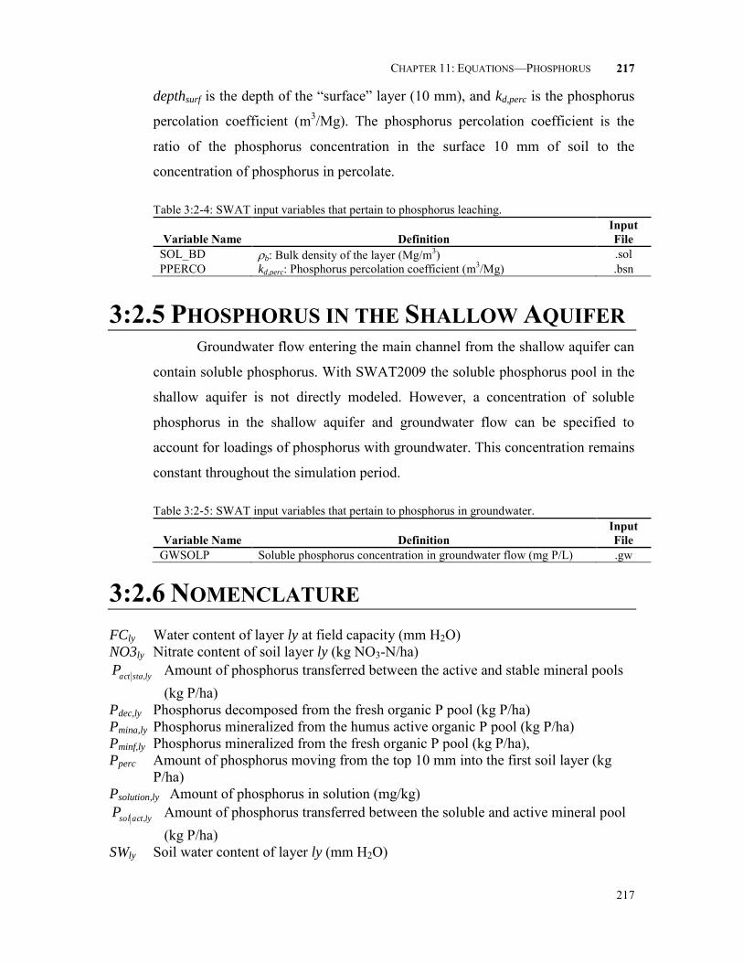
CHAPTER 11: EQUATIONS—PHOSPHORUS
217
217
depthsurf is the depth of the “surface” layer (10 mm), and kd,perc is the phosphorus
percolation coefficient (m3/Mg). The phosphorus percolation coefficient is the
ratio of the phosphorus concentration in the surface 10 mm of soil to the
concentration of phosphorus in percolate.
Table 3:2-4: SWAT input variables that pertain to phosphorus leaching.
Variable Name
Definition Input File
SOL_BD b: Bulk density of the layer (Mg/m3) .sol PPERCO kd,perc: Phosphorus percolation coefficient (m3/Mg) .bsn
3:2.5 PHOSPHORUS IN THE SHALLOW AQUIFER Groundwater flow entering the main channel from the shallow aquifer can
contain soluble phosphorus. With SWAT2009 the soluble phosphorus pool in the
shallow aquifer is not directly modeled. However, a concentration of soluble
phosphorus in the shallow aquifer and groundwater flow can be specified to
account for loadings of phosphorus with groundwater. This concentration remains
constant throughout the simulation period.
Table 3:2-5: SWAT input variables that pertain to phosphorus in groundwater.
Variable Name
Definition Input File
GWSOLP Soluble phosphorus concentration in groundwater flow (mg P/L) .gw
3:2.6 NOMENCLATURE FCly Water content of layer ly at field capacity (mm H2O) NO3ly Nitrate content of soil layer ly (kg NO3-N/ha)
lystaactP , Amount of phosphorus transferred between the active and stable mineral pools
(kg P/ha) Pdec,ly Phosphorus decomposed from the fresh organic P pool (kg P/ha) Pmina,ly Phosphorus mineralized from the humus active organic P pool (kg P/ha) Pminf,ly Phosphorus mineralized from the fresh organic P pool (kg P/ha), Pperc Amount of phosphorus moving from the top 10 mm into the first soil layer (kg
P/ha) Psolution,ly Amount of phosphorus in solution (mg/kg)
lyactsolP , Amount of phosphorus transferred between the soluble and active mineral pool
(kg P/ha) SWly Soil water content of layer ly (mm H2O)

218 SWAT THEORETICAL DOCUMENTATION, VERSION 2009
218
Tsoil,ly Temperature of layer ly (C)
concP Concentration of phosphorus in a layer (mg/kg or ppm) depthly Depth of the layer (mm) kd,perc Phosphorus percolation coefficient (m3/Mg) minPact,ly Amount of phosphorus in the active mineral pool (mg/kg or kg P/ha) minPsta,ly Amount of phosphorus in the stable mineral pool (mg/kg or kg P/ha) orgNact,ly Nitrogen in the active organic pool in layer ly (mg/kg or kg N/ha) orgNfrsh,ly Nitrogen in the fresh organic pool in layer ly (kg N/ha) orgNhum,ly Amount of nitrogen in humic organic pool in the layer (mg/kg or kg N/ha) orgNsta,ly Nitrogen in the stable organic pool in layer ly (mg/kg or kg N/ha) orgPact,ly Amount of phosphorus in the active organic pool (kg P/ha) orgPfrsh,ly Phosphorus in the fresh organic pool in layer ly (kg P/ha) orgPhum,ly Amount of phosphorus in humic organic pool in the layer (mg/kg or kg P/ha) orgPsta,ly Amount of phosphorus in the stable organic pool (kg P/ha) pai Phosphorus availability index
rsdly Residue in layer ly (kg/ha) wperc,ly Amount of water percolating to the underlying soil layer on a given day (mm
H2O)
eqP Slow equilibration rate constant (0.0006 d-1) min Rate coefficient for mineralization of the humus active organic nutrients rsd Rate coefficient for mineralization of the residue fresh organic nutrients ntr,ly Residue decay rate constant C:N Residue C:N ratio in the soil layer C:P Residue C:P ratio in the soil layer ntr,ly Nutrient cycling residue composition factor for layer ly sw,ly Nutrient cycling water factor for layer ly tmp,ly Nutrient cycling temperature factor for layer ly b Bulk density of the layer (Mg/m3)
3:2.7 REFERENCES
Barrow, N.J. and T.C. Shaw. 1975. The slow reactions between soil and anions. 2.
Effect of time and temperature on the decrease in phosphate concentration
in soil solution. Soil Sci. 119:167-177.
Cope, J.T., C.E. Evans, and H.C. Williams. 1981. Soil test fertility
recommendations for Alabama crops. Alabama Agric. Station Circular
No. 251.

CHAPTER 11: EQUATIONS—PHOSPHORUS
219
219
Jones, C.A. C.V. Cole, A.N. Sharpley, and J.R. Williams. 1984. A simplified soil
and plant phosphorus model. I. Documentation. Soil Sci. Soc. Am. J.
48:800-805.
Munns, D.N. and R.L. Fox. 1976. The slow reaction which continues after
phosphate adsorption: Kinetics and equilibrium in some tropical soils. Soil
Sci. Soc. Am. J. 40:46-51.
Rajan, S.S.S. and R.L. Fox. 1972. Phosphate adsorption by soils. 1. Influence of
time and ionic environment on phosphate adsorption. Commun. Soil. Sci.
Plant Anal. 3:493-504.
Sharpley, A.N. 1982. A prediction of the water extractable phosphorus content of
soil following a phosphorus addition. J. Environ. Qual. 11:166-170.
Sharpley, A.N., C. Gray, C.A. Jones, and C.V. Cole. 1984. A simplified soil and
plant phosphorus model. II. Prediction of labile, organic, and sorbed P
amounts. Soil Sci. Soc. Am. J. 48:805-809.
Sharpley, A.N. and J.K. Syers. 1979. Phosphorus inputs into a stream draining an
agricultural watershed: II. Amounts and relative significance of runoff
types. Water, Air and Soil Pollution 11:417-428.

220 SWAT THEORETICAL DOCUMENTATION, VERSION 2009
220

221
SECTION 3 CHAPTER 3
EQUATIONS:
PESTICIDES
One of the primary purposes of tillage and harvesting practices in early
farming systems was to remove as much plant residue from the field as possible
so that pests had no food source to sustain them until the next growing season. As
research linked erosion to lack of soil cover, farmers began to perform fewer
tillage operations and altered harvesting methods to leave more residue. As
mechanical methods of pest control were minimized or eliminated, chemical
methods of pest control began to assume a key role in the management of
unwanted organisms.
Pesticides are toxic by design, and there is a natural concern about the
impact of their presence in the environment on human health and environmental
quality. The fate and transport of a pesticide are governed by properties such as
solubility in water, volatility and ease of degradation. The algorithms in SWAT

222 SWAT THEORETICAL DOCUMENTATION, VERSION 2009
222
used to model pesticide movement and fate are adapted from GLEAMS (Leonard
et al., 1987).
Pesticide may be aerially applied to an HRU with some fraction
intercepted by plant foliage and some fraction reaching the soil. Pesticide may
also be incorporated into the soil through tillage. SWAT monitors pesticide
amounts on foliage and in all soil layers. Figure 3:3-1 shows the potential
pathways and processes simulated in SWAT.
Figure 3:3-1: Pesticide fate and transport in SWAT.
3:3.1 WASH-OFF A portion of the pesticide on plant foliage may be washed off during rain
events. The fraction washed off is a function of plant morphology, pesticide
solubility, and the timing and intensity of the rainfall event. Wash-off will occur
when the amount of precipitation on a given day exceeds 2.54 mm.
The amount of pesticide washing off plant foliage during a precipitation
event on a given day is calculated:
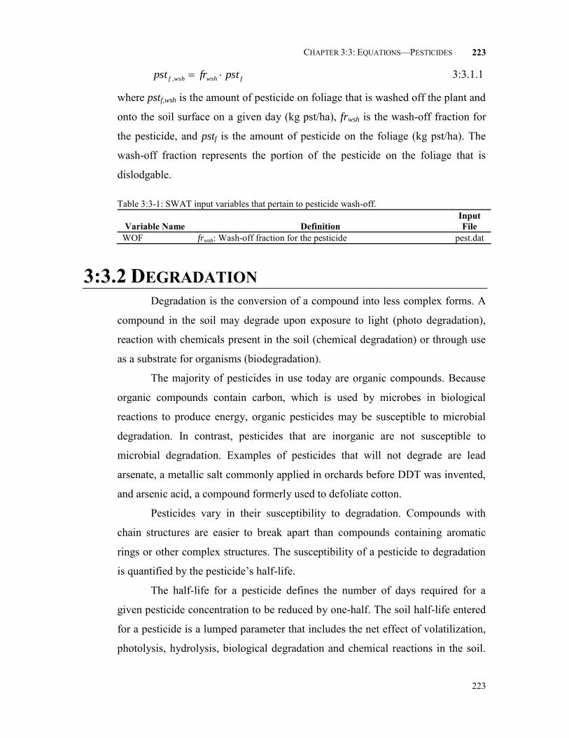
CHAPTER 3:3: EQUATIONS—PESTICIDES
223
223
fwshwshf pstfrpst , 3:3.1.1
where pstf,wsh is the amount of pesticide on foliage that is washed off the plant and
onto the soil surface on a given day (kg pst/ha), frwsh is the wash-off fraction for
the pesticide, and pstf is the amount of pesticide on the foliage (kg pst/ha). The
wash-off fraction represents the portion of the pesticide on the foliage that is
dislodgable.
Table 3:3-1: SWAT input variables that pertain to pesticide wash-off.
Variable Name
Definition Input File
WOF frwsh: Wash-off fraction for the pesticide pest.dat
3:3.2 DEGRADATION Degradation is the conversion of a compound into less complex forms. A
compound in the soil may degrade upon exposure to light (photo degradation),
reaction with chemicals present in the soil (chemical degradation) or through use
as a substrate for organisms (biodegradation).
The majority of pesticides in use today are organic compounds. Because
organic compounds contain carbon, which is used by microbes in biological
reactions to produce energy, organic pesticides may be susceptible to microbial
degradation. In contrast, pesticides that are inorganic are not susceptible to
microbial degradation. Examples of pesticides that will not degrade are lead
arsenate, a metallic salt commonly applied in orchards before DDT was invented,
and arsenic acid, a compound formerly used to defoliate cotton.
Pesticides vary in their susceptibility to degradation. Compounds with
chain structures are easier to break apart than compounds containing aromatic
rings or other complex structures. The susceptibility of a pesticide to degradation
is quantified by the pesticide’s half-life.
The half-life for a pesticide defines the number of days required for a
given pesticide concentration to be reduced by one-half. The soil half-life entered
for a pesticide is a lumped parameter that includes the net effect of volatilization,
photolysis, hydrolysis, biological degradation and chemical reactions in the soil.

224 SWAT THEORETICAL DOCUMENTATION, VERSION 2009
224
Because pesticide on foliage degrades more rapidly than pesticide in the soil,
SWAT allows a different half-life to be defined for foliar degradation.
Pesticide degradation or removal in all soil layers is governed by first-
order kinetics:
tkpstpst soilpolystlys ,,,,, exp 3:3.2.1
where psts,ly,t is the amount of pesticide in the soil layer at time t (kg pst/ha),
psts,ly,o is the initial amount of pesticide in the soil layer (kg pst/ha), kp,soil is the
rate constant for degradation or removal of the pesticide in soil (1/day), and t is
the time elapsed since the initial pesticide amount was determined (days). The
rate constant is related to the soil half-life as follows:
soilp
sk
t,
,21693.0
3:3.2.2
where t1/2,s is the half-life of the pesticide in the soil (days).
The equation governing pesticide degradation on foliage is:
tkpstpst foliarpoftf ,,, exp 3:3.2.3
where pstf,t is the amount of pesticide on the foliage at time t (kg pst/ha), pstf,o is
the initial amount of pesticide on the foliage (kg pst/ha), kp,foliar is the rate constant
for degradation or removal of the pesticide on foliage (1/day), and t is the time
elapsed since the initial pesticide amount was determined (days). The rate
constant is related to the foliar half-life as follows:
foliarp
fk
t,
,21693.0
3:3.2.4
where t1/2,f is the half-life of the pesticide on foliage (days).
Table 3:3-2: SWAT input variables that pertain to pesticide degradation.
Variable Name
Definition Input File
HLIFE_S t1/2,s: Half-life of the pesticide in the soil (days) pest.dat HLIFE_F t1/2,f: Half-life of the pesticide on foliage (days) pest.dat

CHAPTER 3:3: EQUATIONS—PESTICIDES
225
225
3:3.3 LEACHING Highly water-soluble pesticides can be transported with percolation deep
into the soil profile and potentially pollute shallow groundwater systems. The
algorithms used by SWAT to calculated pesticide leaching simultaneously solve
for loss of pesticide in surface runoff and lateral flow also. These algorithms are
reviewed in Chapter 4:3.
3:3.4 NOMENCLATURE
frwsh Wash-off fraction for the pesticide kp,foliar Rate constant for degradation or removal of the pesticide on foliage (1/day) kp,soil Rate constant for degradation or removal of the pesticide in soil (1/day) pstf Amount of pesticide on the foliage (kg pst/ha) pstf,wsh Amount of pesticide on foliage that is washed off the plant and onto the soil
surface on a given day (kg pst/ha) psts,ly Amount of pesticide in the soil (kg pst/ha) t Time elapsed since the initial pesticide amount was determined (days) t1/2,f Half-life of the pesticide on foliage (days) t1/2,s Half-life of the pesticide in the soil (days)
3:3.5 REFERENCES
Leonard, R.A., W.G. Knisel., and D.A. Still. 1987. GLEAMS: Groundwater
loading effects of agricultural management systems. Trans. ASAE.
30:1403-1418.

226 SWAT THEORETICAL DOCUMENTATION, VERSION 2009
226
227
SECTION 3 CHAPTER 4
EQUATIONS:
BACTERIA
Contamination of drinking water by pathogenic organisms is a major
environmental concern. Similar to water pollution by excess nutrients, water
pollution by microbial pathogens can also be caused by point and nonpoint
sources. Point source water contamination normally results from a direct entry of
wastewater from municipal or water treatment systems into a drinking water
supply. Nonpoint sources of bacterial pollution can be difficult to identify as they
can originate from animal production units, land application of different manure
types, and wildlife.
Although there are many potential sources of pathogenic loadings to
streams, agronomic practices that utilize animal manures contaminated with
pathogenic or parasitic organisms appear to be the major source of nonpoint
contamination in watersheds. In recent years, a concentration of animal feeding
operations has occurred in the cattle, swine and poultry production industries.

228 SWAT THEORETICAL DOCUMENTATION, VERSION 2009
228
These operations generate substantial amounts of animal manure that are normally
applied raw to relatively limited land areas. Even though animal manure can be
considered a beneficial fertilizer and soil amendment, high rates of land applied
raw manure increase the risk of surface or groundwater contamination, both from
excess nutrients and pathogenic organisms such as Cryptosporidium, Salmonella,
or Escherichia coli 0157:H7.
Fecal coliforms (generic forms of bacteria) have customarily been used as
indicators of potential pathogen contamination for both monitoring and modeling
purposes (Baudart et al., 2000; Hunter et al., 2000; Pasquarell and Boyer, 1995;
Walker et al., 1990; Stoddard et al., 1998; Moore et al., 1988). However, recent
studies have documented waterborne disease outbreaks caused by
Cryptosporidium, Norwalk and hepatitis A viruses, and salmonella despite
acceptably low levels of indicator bacteria (Field et al, 1996).
SWAT considers fecal coliform an indicator of pathogenic organism
contamination. However, to account for the presence of serious pathogens that
may follow different growth/die-off patterns, SWAT allows two species or strains
of pathogens with distinctly different die-off/re-growth rates to be defined. The
two-population modeling approach is used to account for the long-term impacts of
persistent bacteria applied to soils, whose population density when initially
applied may be insignificant compared to that of less persistent bacteria.
One or two bacteria populations may be introduced into an HRU through
one of the three types of fertilizer applications reviewed in Chapter 6:1. When
bacteria in manure are applied to an HRU, some fraction is intercepted by plant
foliage with the remainder reaching the soil. SWAT monitors the two bacteria
populations on foliage and in the top 10 mm of soil that interacts with surface
runoff. Bacteria in the surface soil layer may be in solution or associated with the
solid phase. Bacteria incorporated deeper into the soil through tillage or transport
with percolating water is assumed to die.

CHAPTER 3:4: EQUATIONS—BACTERIA
229
229
3:4.1 WASH-OFF A portion of the bacteria on plant foliage may be washed off during rain
events. The fraction washed off is a function of plant morphology, bacteria
characteristics, and the timing and intensity of the rainfall event. Wash-off will
occur when the amount of precipitation on a given day exceeds 2.54 mm.
The amount of bacteria washing off plant foliage during a precipitation
event on a given day is calculated:
follplpwshwshlp bactfrbact ,,, 3:4.1.1
folppwshwshp bactfrbact ,,, 3:4.1.2
where bactlp,wsh is the amount of less persistent bacteria on foliage that is washed
off the plant and onto the soil surface on a given day (# cfu/m2), bactp,wsh is the
amount of persistent bacteria on foliage that is washed off the plant and onto the
soil surface on a given day (# cfu/m2), frwsh,lp is the wash-off fraction for the less
persistent bacteria, frwsh,p is the wash-off fraction for the persistent bacteria,
bactlp,fol is the amount of less persistent bacteria attached to the foliage (# cfu/m2),
and bactp,fol is the amount of persistent bacteria attached to the foliage (# cfu/m2).
The wash-off fraction represents the portion of the bacteria on the foliage that is
dislodgable.
Bacteria that washes off the foliage is assumed to remain in solution in the
soil surface layer.
Table 3:4-1: SWAT input variables that pertain to bacteria wash-off.
Variable Name
Definition Input File
WOF_P frwsh,p: Wash-off fraction for persistent bacteria .bsn WOF_LP frwsh,lp: Wash-off fraction for less persistent bacteria .bsn
3:4.2 BACTERIA DIE-OFF/RE-GROWTH Chick’s Law first order decay equation is used to determine the quantity of
bacteria removed from the system through die-off and added to the system by
regrowth. The equation for die-off/re-growth was taken from Reddy et al. (1981)
as modified by Crane and Moore (1986) and later by Moore et al. (1989). The

230 SWAT THEORETICAL DOCUMENTATION, VERSION 2009
230
equation was modified in SWAT to include a user-defined minimum daily loss.
Die-off/re-growth is modeled for the two bacteria populations on foliage, in the
surface soil solution and sorbed to surface soil particles. The equations used to
calculate daily bacteria levels in the different pools are:
lpnetlpfolilpfolilpfol bactbactbact min,,1,, exp 3:4.2.1
pnetpfolipfolipfol bactbactbact min,,1,, exp 3:4.2.2
lpnetlpsolilpsolilpsol bactbactbact min,,1,, exp 3:4.2.3
pnetpsolipsolipsol bactbactbact min,,1,, exp 3:4.2.4
lpnetlpsorbilpsorbilpsorb bactbactbact min,,1,, exp 3:4.2.5
pnetpsorbipsorbipsorb bactbactbact min,,1,, exp 3:4.2.6
where bactlpfol,i is the amount of less persistent bacteria present on foliage on day i
(#cfu/m2), bactlpfol,i-1 is the amount of less persistent bacteria present on foliage on
day i-1 (#cfu/m2), μlpfol,net is the overall rate constant for die-off/re-growth of less
persistent bacteria on foliage (1/day), bactmin,lp is the minimum daily loss of less
persistent bacteria (#cfu/m2), bactpfol,i is the amount of persistent bacteria present
on foliage on day i (#cfu/m2), bactpfol,i-1 is the amount of persistent bacteria
present on foliage on day i-1 (#cfu/m2), μpfol,net is the overall rate constant for die-
off/re-growth of persistent bacteria on foliage (1/day), bactmin,p is the minimum
daily loss of persistent bacteria (#cfu/m2), bactlpsol,i is the amount of less persistent
bacteria present in soil solution on day i (#cfu/m2), bactlpsol,i-1 is the amount of less
persistent bacteria present in soil solution on day i-1 (#cfu/m2), μlpsol,net is the
overall rate constant for die-off/re-growth of less persistent bacteria in soil
solution (1/day), bactpsol,i is the amount of persistent bacteria present in soil
solution on day i (#cfu/m2), bactpsol,i-1 is the amount of persistent bacteria present
in soil solution on day i-1 (#cfu/m2), μpsol,net is the overall rate constant for die-
off/re-growth of persistent bacteria in soil solution (1/day), bactlpsorb,i is the
amount of less persistent bacteria sorbed to the soil on day i (#cfu/m2), bactlpsorb,i-1
is the amount of less persistent bacteria sorbed to the soil on day i-1 (#cfu/m2),
μlpsorb,net is the overall rate constant for die-off/re-growth of less persistent bacteria
sorbed to the soil (1/day), bactpsorb,i is the amount of persistent bacteria sorbed to

CHAPTER 3:4: EQUATIONS—BACTERIA
231
231
the soil on day i (#cfu/m2), bactpsorb,i-1 is the amount of persistent bacteria sorbed
to the soil on day i-1 (#cfu/m2), and μpsorb,net is the overall rate constant for die-
off/re-growth of persistent bacteria sorbed to the soil (1/day).
The overall rate constants define the net change in bacterial population for
the different pools modeled. The impact of temperature effects on bacteria die-
off/re-growth were accounted for using equations proposed by Mancini (1978).
The user defines the die-off and growth factors for the two bacterial populations
in the different pools at 20C. The overall rate constants at 20C are then
calculated:
20,,20,,20,, grwlpfoldielpfolnetlpfol 3:4.2.7
20,,20,,20,, grwpfoldiepfolnetpfol 3:4.2.8
20,,20,,20,, grwlpsoldielpsolnetlpsol 3:4.2.9
20,,20,,20,, grwpsoldiepsolnetpsol 3:4.2.10
20,,20,,20,, grwlpsorbdielpsorbnetlpsorb 3:4.2.11
20,,20,,20,, grwpsorbdiepsorbnetpsorb 3:4.2.12
where μlpfol,net,20 is the overall rate constant for die-off/re-growth of less persistent
bacteria on foliage at 20C (1/day), μlpfol,die,20 is the rate constant for die-off of less
persistent bacteria on foliage at 20C (1/day), μlpfol,grw,20 is the rate constant for re-
growth of less persistent bacteria on foliage at 20C (1/day), μpfol,net,20 is the
overall rate constant for die-off/re-growth of persistent bacteria on foliage at 20C
(1/day), μpfol,die,20 is the rate constant for die-off of persistent bacteria on foliage at
20C (1/day), μpfol,grw,20 is the rate constant for re-growth of persistent bacteria on
foliage at 20C (1/day), μlpsol,net,20 is the overall rate constant for die-off/re-growth
of less persistent bacteria in soil solution at 20C (1/day), μlpsol,die,20 is the rate
constant for die-off of less persistent bacteria in soil solution at 20C (1/day),
μlpsol,grw,20 is the rate constant for re-growth of less persistent bacteria in soil
solution at 20C (1/day), μpsol,net,20 is the overall rate constant for die-off/re-growth
of persistent bacteria in soil solution at 20C (1/day), μpsol,die,20 is the rate constant
for die-off of persistent bacteria in soil solution at 20C (1/day), μpsol,grw,20 is the

232 SWAT THEORETICAL DOCUMENTATION, VERSION 2009
232
rate constant for re-growth of persistent bacteria in soil solution at 20C (1/day),
μlpsorb,net,20 is the overall rate constant for die-off/re-growth of less persistent
bacteria attached to soil particles at 20C (1/day), μlpsorb,die,20 is the rate constant
for die-off of less persistent bacteria attached to soil particles at 20C (1/day),
μlpsorb,grw,20 is the rate constant for re-growth of less persistent bacteria attached to
soil particles at 20C (1/day), μpsorb,net,20 is the overall rate constant for die-off/re-
growth of persistent bacteria attached to soil particles at 20C (1/day), μpsorb,die,20
is the rate constant for die-off of persistent bacteria attached to soil particles at
20C (1/day), and μpsorb,grw,20 is the rate constant for re-growth of persistent
bacteria attached to soil particles at 20C (1/day).
The overall rate constants are adjusted for temperature using the
equations: 20
20,,,
avT
bactnetlpfolnetlpfol 3:4.2.13
2020,,,
avT
bactnetpfolnetpfol 3:4.2.14
2020,,,
avT
bactnetlpsolnetlpsol 3:4.2.15
2020,,,
avT
bactnetpsolnetpsol 3:4.2.16
2020,,,
avT
bactnetlpsorbnetlpsorb 3:4.2.17
2020,,,
avT
bactnetpsorbnetpsorb 3:4.2.18
where θbact is the temperature adjustment factor for bacteria die-off/re-growth, avT
is the mean daily air temperature, and all other terms are as previously defined.

CHAPTER 3:4: EQUATIONS—BACTERIA
233
233
Table 3:4-2: SWAT input variables that pertain to bacteria die-off/re-growth.
Variable Name
Definition Input File
WDPQ μpsol,die,20: Die-off factor for persistent bacteria in soil solution at 20C (1/day)
.bsn
WGPQ μpsol,grw,20: Growth factor for persistent bacteria in soil solution at 20C (1/day)
.bsn
WDLPQ μlpsol,die,20: Die-off factor for less persistent bacteria in soil solution at 20C (1/day)
.bsn
WGLPQ μlpsol,grw,20: Growth factor for less persistent bacteria in soil solution at 20C (1/day)
.bsn
WDPS μpsorb,die,20: Die-off factor for persistent bacteria adsorbed to soil particles at 20C (1/day)
.bsn
WGPS μpsorb,grw,20: Growth factor for persistent bacteria adsorbed to soil particles at 20C (1/day)
.bsn
WDLPS μlpsorb,die,20: Die-off factor for less persistent bacteria adsorbed to soil particles at 20C (1/day)
.bsn
WGLPS μlpsorb,grw,20: Growth factor for less persistent bacteria adsorbed to soil particles at 20C (1/day)
.bsn
WDPF μpfol,die,20: Die-off factor for persistent bacteria on foliage at 20C (1/day)
.bsn
WGPF μpfol,grw,20: Growth factor for persistent bacteria on foliage at 20C (1/day)
.bsn
WDLPF μlpfol,die,20: Die-off factor for less persistent bacteria on foliage at 20C (1/day)
.bsn
WGLPF μlpfol,grw,20: Growth factor for less persistent bacteria on foliage at 20C (1/day)
.bsn
THBACT θbact: Temperature adjustment factor for bacteria die-off/growth .bsn BACTMINLP bactmin,lp: Minimum daily loss of less persistent bacteria (#
cfu/m2) .bsn
BACTMINP bactmin,p: Minimum daily loss of persistent bacteria (# cfu/m2) .bsn
3:4.3 LEACHING Bacteria can be transported with percolation into the soil profile. Only
bacteria present in the soil solution is susceptible to leaching. Bacteria removed
from the surface soil layer by leaching are assumed to die in the deeper soil
layers.
The amount of bacteria transported from the top 10 mm into the first soil
layer is:
percbactsurfb
surfperclpsol
perclpkdepth
wbactbact
,
,, 10
3:4.3.1
percbactsurfb
surfpercpsol
percpkdepth
wbactbact
,
,, 10
3:4.3.2

234 SWAT THEORETICAL DOCUMENTATION, VERSION 2009
234
where bactlp,perc is the amount of less persistent bacteria transported from the top
10 mm into the first soil layer (#cfu/m2), bactlpsol is the amount of less persistent
bacteria present in soil solution (#cfu/m2), wperc,surf is the amount of water
percolating to the first soil layer from the top 10 mm on a given day (mm H2O),
b is the bulk density of the top 10 mm (Mg/m3) (assumed to be equivalent to bulk
density of first soil layer), depthsurf is the depth of the “surface” layer (10 mm),
kbact,perc is the bacteria percolation coefficient (10 m3/Mg), bactp,perc is the amount
of persistent bacteria transported from the top 10 mm into the first soil layer
(#cfu/m2), and bactpsol is the amount of persistent bacteria present in soil solution
(#cfu/m2).
Table 3:4-3: SWAT input variables that pertain to bacteria transport in percolate.
Variable Name
Definition Input File
SOL_BD b: Bulk density of the layer (Mg/m3) .sol BACTMIX kbact,perc: Bacteria percolation coefficient (10 m3/Mg) .bsn
3:4.4 NOMENCLATURE
avT Mean air temperature for day (C) bactlp,fol Amount of less persistent bacteria attached to the foliage (# cfu/m2) bactlp,perc Amount of less persistent bacteria transported from the top 10 mm into the first
soil layer (#cfu/m2) bactlpsol Amount of less persistent bacteria present in soil solution (#cfu/m2) bactlpsorb Amount of less persistent bacteria sorbed to the soil (#cfu/m2) bactlp,wsh Amount of less persistent bacteria on foliage that is washed off the plant and
onto the soil surface on a given day (# cfu/m2) bactmin Minimum daily loss of bacteria (#cfu/m2) bactp,fol Amount of persistent bacteria attached to the foliage (# cfu/m2) bactp,perc Amount of persistent bacteria transported from the top 10 mm into the first soil
layer (#cfu/m2) bactpsol Amount of persistent bacteria present in soil solution (#cfu/m2) bactpsorb Amount of persistent bacteria sorbed to the soil (#cfu/m2) bactp,wsh Amount of persistent bacteria on foliage that is washed off the plant and onto the
soil surface on a given day (# cfu/m2) depthly Depth of the layer (mm) frwsh,lp Wash-off fraction for the less persistent bacteria frwsh,p Wash-off fraction for the persistent bacteria kbact,perc Bacteria percolation coefficient (10 m3/Mg)

CHAPTER 3:4: EQUATIONS—BACTERIA
235
235
wperc,ly Amount of water percolating to the underlying soil layer on a given day (mm H2O)
b Bulk density of the layer (Mg/m3) μlpfol,die,20 Rate constant for die-off of less persistent bacteria on foliage at 20C (1/day) μlpfol,grw,20 Rate constant for re-growth of less persistent bacteria on foliage at 20C
(1/day) μlpfol,net Overall rate constant for die-off/re-growth of less persistent bacteria on foliage
(1/day) μlpfol,net,20 Overall rate constant for die-off/re-growth of less persistent bacteria on foliage
at 20C (1/day) μlpsol,die,20 Rate constant for die-off of less persistent bacteria in soil solution at 20C
(1/day) μlpsol,grw,20 Rate constant for re-growth of less persistent bacteria in soil solution at 20C
(1/day) μlpsol,net Overall rate constant for die-off/re-growth of less persistent bacteria in soil
solution (1/day) μlpsol,net,20 Overall rate constant for die-off/re-growth of less persistent bacteria in soil
solution at 20C (1/day) μlpsorb,die,20 Rate constant for die-off of less persistent bacteria attached to soil particles at
20C (1/day) μlpsorb,grw,20 Rate constant for re-growth of less persistent bacteria attached to soil particles
at 20C (1/day) μlpsorb,net Overall rate constant for die-off/re-growth of less persistent bacteria sorbed to
the soil (1/day) μlpsorb,net,20 Overall rate constant for die-off/re-growth of less persistent bacteria attached
to soil particles at 20C (1/day) μpfol,die,20 Rate constant for die-off of persistent bacteria on foliage at 20C (1/day) μpfol,grw,20 Rate constant for re-growth of persistent bacteria on foliage at 20C (1/day) μpfol,net Overall rate constant for die-off/re-growth of persistent bacteria on foliage (1/day) μpfol,net,20 Overall rate constant for die-off/re-growth of persistent bacteria on foliage at
20C (1/day) μpsol,die,20 Rate constant for die-off of persistent bacteria in soil solution at 20C (1/day) μpsol,grw,20 Rate constant for re-growth of persistent bacteria in soil solution at 20C
(1/day) μpsol,net Overall rate constant for die-off/re-growth of persistent bacteria in soil solution
(1/day) μpsol,net,20 Overall rate constant for die-off/re-growth of persistent bacteria in soil solution
at 20C (1/day) μpsorb,die,20 Rate constant for die-off of persistent bacteria attached to soil particles at 20C
(1/day) μpsorb,grw,20 Rate constant for re-growth of persistent bacteria attached to soil particles at
20C (1/day) μpsorb,net Overall rate constant for die-off/re-growth of persistent bacteria sorbed to the soil
(1/day)

236 SWAT THEORETICAL DOCUMENTATION, VERSION 2009
236
μpsorb,net,20 Overall rate constant for die-off/re-growth of persistent bacteria attached to soil particles at 20C (1/day)
θbact Temperature adjustment factor for bacteria die-off/re-growth
3:4.5 REFERENCES
Baudart, J., J. Grabulos, J.P. Barusseau, and P. Lebaron. 2000. Salmonella spp. and fecal coliform loads in coastal waters from point vs. nonpoint sources of pollution. J. Environ. Qual. 29:241-250.
Crane, S.R. and J.A. Moore. 1986. Modeling enteric bacterial die-off: a review. Water, Air, and Soil Pollution 27: 411-439.
Field, R., M. Borst, M. Stinson, C. Fan, J. Perdek, D. Sullivan, and T. O’Conner. 1996. Risk management research plan for wet weather flows. National Risk Management Research Laboratory, EPA/600/R-96/140. Cincinnati.
Hunter, C., J. Perkins, J. Tranter, and P. Hardwick. 2000. Fecal bacteria in the waters of an upland area in Derbyshire, England: The influence of agricultural land use. J. Environ. Qual. 29: 1253-1261.
Mancini, J.L. 1978. Numerical estimates of coliform mortality rates under various conditions. J. Water Poll. Cont. Fed. 50: 2477-2484.
Moore, J.A., J.D. Smyth, E.S. Baker, and J.R. Miner. 1988. Evaluating coliform concentrations in runoff from various animal waste management systems. Special Report 817. Agricultural Experiment Stations, Oregon State University, Corvallis.
Moore, J.A., J.D. Smyth, E.S. Baker, J.R. Miner, and D.C. Moffit. 1989. Modeling bacteria movement in livestock manure systems. Trans. ASAE 32: 1049-1053.
Pasquarell, G.C. and D.G. Boyer. 1995. Agricultural impacts on bacterial water quality in karst groundwater. J. Environ. Qual. 24: 959-969.
Reddy, K.R., R. Khaleel, and M.R. Overcash. 1981. Behavior and transport of microbial pathogens and indicator organisms in soils treated with organic wastes. J. Environ. Qual. 10: 255-266.
Stoddard, C.S., M.S. Coyne, and J.H. Grove. 1998. Fecal bacteria survival and infiltration through a shallow agricultural soil: Timing and tillage effects. J. Environ. Qual. 27: 1516-1523.
Walker, S.E., S. Mostaghimi, T.A. Dillaha, and F.E. Woeste. 1990. Modeling animal waste management practices: Impacts on bacteria levels in runoff from agricultural lands. Trans. ASAE 33: 807-817.

CHAPTER 3:4: EQUATIONS—BACTERIA
237
237

238
SECTION 3 CHAPTER 5
EQUATIONS:
CARBON
Land use changes and the intensification of agricultural production have
dramatically altered the flow of nutrients resulting in unprecedented
transcontinental inter-watershed and intra-watershed transfers of nitrogen (N),
phosphorus (P), and other nutrients with fertilizer, harvest product, and pollutant
flow (Galloway et al., 2008). Nutrient cycling in soils plays a major role in the
control of these flows. Carbon (C), N, and P cycling are intimately linked through
soil, plant and microbial processes. These processes affect the level of inorganic
N and P and the C:N and C:P ratios of SOM. To realistically represent these C, N,
and P transfers in river-basin scale models such as the Soil Water Assessment
Tool (SWAT, Arnold et al., 1998). a comprehensive integration of the cycling of
these nutrients through soil organic matter (SOM) is required.
Most conceptual and quantitative SOM cycling models compartmentalize
soil C and N in pools with different, yet stable, turnover rates and C:N ratios (Paul
CHAPTER 3:5: EQUATIONS—CARBON
239
239
et al., 2006, McGill et al., 1981; Parton et al., 1988; Verberne et al., 1990).
Incubation experiments also suggest the existence of pools with varying turnover
rates (e.g. Collins et al, 2000); however, Six et al. (2002) indicated after an
extensive literature review that the success at matching measurable and modelable
SOM pools has been minimal. Furthermore, the division of SOM in pools has
been criticized on mathematical grounds, as continuous turnover rates
distributions can be artificially represented by discrete pools (Bruun and Luxhoi,
2006). These criticisms do not deny the existence of pools but rather emphasize
the difficulty in establishing generalized methods to measure or predict their size
and turnover rate. This unpredictability can limit the applicability of multi-pool
SOM sub-models if the parameterization for different agricultural soils,
pasturelands, forestlands and organic soils is uncertain or requires intensive
calibration.
In this chapter, we describe the one-pool SOM sub-model implemented in
SWAT. This sub-model is conceptually based on the model described in
Kemanian and Stockle (2010), and was adapted to the SWAT algorithms and
integrated to the cycling of N and P.
3:5.1 SUB-MODEL DESCRIPTION
The sub-model described here pertains to soil processes at the hydrologic
unit response level. The new sub-model has one pool for soil organic C, N, and P
(SC, SN, SP, respectively, kg m-2), and separate pools for residue and manure C, N,
and P (RC, RN, RP and MC, MN, MP, respectively, kg m-2). The pools are not
separated in active and stable pools. Microbial activity on SOM, manure, and
residues decomposes simultaneously the organic C, N, and P. Decomposition of
residues may add to (mineralization) or subtract from (immobilization) the
inorganic N and P pools, depending on the C:N and C:P ratio of the decomposing
pools (RCN, RCP, MCN, and MCP, respectively) and those of the SOM or destiny
pool (SCN, SCP), and on the humification rate (h). The humification rate represents
the fraction of C in the decomposing residues that are effectively incorporated in

240 SWAT THEORETICAL DOCUMENTATION, VERSION 2009
240
the SC pool, the reminder being respired as CO2. The balance equations for each
soil layer for the organic residue, manure, and soil pools are as follows.
Residue and manure pools (represented as R and M) gain mass through
additions (IR and IM for residue and manure, respectively) and lose mass from
decomposition following first order kinetics:
, 3:5.1.1a
, 3:5.1.1b
( ) , 3:5.1.1c
where fE is the combined effect of the soil factors temperature (fT), moisture (fW),
and aeration (fO), fp (0.67) is a power regulating the multiplicative effect of the
three environmental factors, and kR (0.05 day-1) and kM (0.025 day-1) are the
optimum decomposition rate (day-1) for residues and manure, respectively. The
addition of residues (or manures) from different sources are bulked with the
existing pool and not tracked separately, with rates shown above assumed to
apply to all sources. If these decomposition rates are made residue- or manure-
specific, every time there is an addition of residues or manure the effective
decomposition rates would have to be calculated as weighted averages of the rate
of the already decomposing pools and that attributed to the newly added
materials, with a weighting function that should change over time, or each pool
tracked separately, both rather impractical propositions.
For the soil pools, the differential equations are as follows:
, 3:5.1.2a
, 3:5.1.2b
where hR and hM are the residue and manure humification rates (kg kg-1) and kS is
the apparent organic matter decomposition rate (day-1). The humification rates
depend on the current SC and a reference SC (SCC):
( (
) ), 3:5.1.3a
( ),
, 3:5.1.3b
( ) 3:5.1.4

CHAPTER 3:5: EQUATIONS—CARBON
241
241
Clay is the soil layer clay fraction (kg clay kg-1 dry soil), SBD is the soil
layer bulk density (kg m-3), and Zl is the soil layer thickness (m). The constant α
(default α = 6) modulates the response of the humification the current SC. The
maximum attainable residue humification is approximately 0.18 kg kg-1. The
same humification is used for below and aboveground residues. The humification
of C from manure was assumed to be 60% higher than that of fresh residues
(approximately 0.29 kg kg-1). The reference SC or SCC depends linearly on the soil
layer clay fraction (Eq. 3:5.1.4) as proposed by Hassink and Whitmore (1997).
When SC = SCC then the humification is 0 and no accumulation of SC above SCC
can occur (Kemanian and Stockle, 2010). In addition, this approach assumes a
dependence of humification on the clay fraction, a dependence represented in
many different ways in other models (e.g. Jenkinson, 1990; Bradbury et al.,
1993). The control of hR and hM in Eq. [3.5.1.3] with α = 6 implies a non-linear
response of hR and hM to SC. It is likely that a better formulation is needed for
these functional equations to apply in organic horizons, tropical soils, or soils with
a high proportion of volcanic ashes.
The C:N ratio of the newly formed organic matter or SCN ranges from 8.5
to 14. The RCN and MCN determine how high SCN can be when there is no mineral
N available that can be an N source for the soil microbes. This estimate of SCN is
reduced depending on the mineral N availability, as follows:
(
(
) )(
( ) ) 3:5.1.5
where Nmin is the mineral N in the layer (mg N kg-1 soil in this equation). The first
term within brackets represents the control of the residues and the second term
represents the control of mineral N on SCN so that the higher the ratio of RCN the
higher the resulting SCN, and the higher the amount of Nmin the lower SCN, with
SCN ranging from 8.5 to 14 kg C kg-1 N in SOM. For manures, MCN substitutes for
RCN and 55 substitutes for the constant 110. The ratio SCP is derived from SCN by
assuming that the newly formed SOM will conserve the N:P ratio of the
decomposing residue and manure. Thus, the C:N and C:P ratios of SOM are not
constant but fluctuates according to these equations during the simulation.

242 SWAT THEORETICAL DOCUMENTATION, VERSION 2009
242
Residues and manure may not supply sufficient N and P to satisfy the SCN
(Eq. 3:5.1.2b) and SCP (Eq. 3:5.1.2c), in which case N and P will be mined from
the inorganic soluble pools. If the inorganic pools cannot supply N and P for
decomposition to proceed, then the decomposition rate of residue and manure is
reduced. Therefore, lack of mineral N and P in solution may slow down
decomposition. The net mineralization is obtained from:
(
), 3:5.1.6a
(
), 3:5.1.6b
where MINRN and MINMN are the net mineralization rates (kg m-2 day-1) from
decomposing residues (Eq. 3:5.1.6a) and manure (Eq. 3:5.1.6b), respectively, with
negative values indicating immobilization and positive values net mineralization.
The same equation applies for P with appropriate C:P ratios. The SOM
decomposition rate (kS) is calculated from:
(
)
. 3:5.1.7
The apparent SC turnover rate (kS) is scaled down from an optimum of 4.5% yr-1
for undisturbed soils (kx = 0.000123 day-1 so that kx × 365 = 0.045) based on
environmental conditions and SC. The power β modulates kS (default β = 0.5) so
that when SC is low, the turnover rate slows sharply. Substituting Eq. 3:5.1.7 for
ks in Eq. 3:5.1.2a with β = 0.5 renders a kinetics of order 3/2 for SC
decomposition, as opposed to the typical first order kinetics commonly use in
SOM decomposition models (see Kemanian and Stockle, 2009). Tillage can
enhance kS through the factor ftool. This factor is calculated independently for each
soil layer and depends on the tillage tool mixing factor (fmix, range 0 to 1) and the
soil texture. The mixing factor and the tillage depth determine the fraction of the
soil layer that is mixed by a tillage operation. The ftool basal value is 1 and it is
enhanced immediately after a tillage event based on the estimated cumulative fmix
(or fcm):
( ) (
). 3:5.1.8

CHAPTER 3:5: EQUATIONS—CARBON
243
243
The factor (ftool) is reduced on a daily basis based on soil moisture to simulate soil
settling. If ftool > 1 and a tillage operation is executed, the corresponding fmix has
to be added to the current fcm. This requires solving for fcm by inverting Eq 3:5.1.6
before recalculating ftool. Since Eq 3:5.1.6 is non-linear on fcm the solution has to
be obtained iteratively. In the SWAT code the solution for fcm has been
approximated by a functional equation to prevent recurrent iterations that can be
computationally expensive. The SOM decomposition always causes net
mineralization to be positive because humification is assumed to be zero. In
actuality, the humification is not zero but since no explicit microbial pool is
considered, the decomposition rate is an apparent decomposition rate that
represents the net loss of C from the SC and underestimates the true turnover rate
of organic C, N, and P (Jenkinson and Parry, 1989).
3:5.2 CHANGES FROM PREVIOUS VERSION
The previous versions of SWAT have separate pools for soil organic N
(two pools, active and stable) and organic P (one pool) and do not include
explicitly SC, RC, or MC pools. Nitrogen and P decompose separately, excepting
the common effect of soil moisture and temperature on the actual decomposition
rate and the indirect control of decomposition through RCN and RCP. The higher
the ratios the lower the decomposition rate, but no immobilization of mineral N or
P occurs. Of the N and P decomposed from residues, 20% is allocated to the
active soil organic N and the soil organic P pools, respectively, and 80% is
allocated to the nitrate (NO3) and P in the soil solution. The 20% allocated to the
N and P organic pools is roughly similar to the humification of C described in the
new sub-model.
In the new sub-model, mineralization of N from organic pools feeds the
NH4 pool instead of the NO3 pool. This will possibly increase volatilization of
ammonium because in SWAT the latter is tightly linked to nitrification. Since
mineralization and immobilization are explicitly calculated, the fluctuations in
mineral NO3, should be more realistically simulated, which has obvious

244 SWAT THEORETICAL DOCUMENTATION, VERSION 2009
244
implications for NO3 transport and other processes across the watershed. Tillage
accelerates SOM turnover and mixes layers according to the tillage depth. In the
previous version tillage had some effects on the surface properties (residue cover)
and mixing only involved two layers. No effect of tillage on the organic N or P
decomposition rate was previously simulated. The new sub-model also enhances
the capacity of SWAT to simulate the impact of tillage on nutrient cycling.
3:5.3 ANALYTICAL SOLUTIONS
The balanced equation for Sc in a single layer (Eq. [3:5.1.2a]) can be
combined with Eq. [3:5.1.3a] and Eq. [3:5.1.7] and with a few assumptions allow
for an analytical solution to the differential equation. The soil clay content and the
C input rate were assumed to be constant and the powers α and β set to 1, so that
the balance equation can be solved explicitly for SC. The time step was considered
to be a year and we assumed that residues and manure fully decompose in that
time frame so that kR = kM = 1. Since the influence of residues and manure on the
SC balance is similar we assumed that C inputs are only through residues. With
these substitutions Eq. [3:5.1.2a] becomes:
3:5.3.1
The constant k substitutes for kxfEftool. This differential equation can be solved
analytically, with integration rendering the following solution:
( )
[(
)√
] 3:5.3.2
√
,
( )
( ) .
The integration constant depends on the initial SC. The steady state solution for
Eq. 3:5.3.2 is:
(√
) 3:5.3.3

CHAPTER 3:5: EQUATIONS—CARBON
245
245
The ratio
is the equilibrium SC that would be obtained if neither hC nor kS
had a dependence on SC. As RC increases, the value of the fraction
will get
smaller. Therefore, the squared root term in Eq. 3:5.3.3 can be approximated as
(
)
by preserving just the first two terms of the binomial expansion, from
which Eq. 3:5.3.4 can be re-written as:
( (
)
) 3:5.3.4
Therefore, as RC increases SC approaches Sx asymptotically (Figure 1). Taking as
a reference a soil layer with Sx = 25 Mg C ha-1, hx = 0.2, and k = 0.01 y-1, it can be
seen in Figure 1 that doubling hx and k have a similar effect but of opposite sign
such that the equilibrium SC increases with increasing hx and decreases with
increasing k. In both cases the increase and the decrease in SC are less than
proportional to the increase in these two parameters. The equilibrium SC,
however, is very sensitive to changes in Sx, which makes this variable critical for
a correct representation of SC dynamics. This formulation is a mathematical
representation of the concept of SC saturation (Hassink and Whitmore, 1997; Six
et al., 2002), enhanced with a control of the decomposition rate by SC.
The transient trajectory of SC is controlled by the quotient of the two
exponential terms in Eq. [3:5.3.5].
∑ ( )
∑ (| | | |)
[3:5.3.5]
For a given Sx and initial SC, increasing the inputs (RC) changes the steady state
SC with decreasing marginal increments as SC approaches Sx, yet the steady state
condition is approached faster with higher inputs (Figure 3:5-1). For a given RC,
changing Sx has a substantial impact on the rate of change of SC when the inputs
are medium to high (Figure 3:5-1) but a minor effect if inputs are too low. This
formulation strongly suggests that soils with higher carbon storage capacity
(higher Sx) that are currently depleted of SC should be the primary targets for
storing SC, or that soils with low Sx may store carbon quickly for a few years but
the rate of gains will decrease earlier than in soils with higher Sx.

246 SWAT THEORETICAL DOCUMENTATION, VERSION 2009
246
The conditions for which the SC can be modeled analytically as shown
here are very restrictive. The numerical solution implemented in the model is
more flexible as the constants α and β are allowed to differ from 1. The model can
be expanded to accommodate saturation of different SOM pools, instead of just
one uniform pool, as strongly suggested by the results and analysis of Stewart et
al. (2008). Yet, this will require a level of parameterization for which we consider
there is simply not sufficient information for a realistic implementation in
numerical models.
Figure 3:5-1: Equilibrium soil organic carbon (SC, Mg C ha-1) for the steady state condition (Eq. [3:5.3.3]) with different values for humification (hx, kg kg-1), SOM apparent turnover rate (k, yr-1), and saturation soil organic carbon (SCC, Mg C ha-1).
The line without a symbol in both panels was arbitrarily chosen as a reference. The linear, no asymptotic line in Panel A shows the equilibrium for the case in which hx and k do not depend on SC so that SC at equilibrium = hxRC/k, where RC is the residue carbon input rate (Mg C ha-1 yr-1). Panel A shows the equilibrium when SCC is doubled and Panel B shows the equilibrium SC when hx or k is doubled.

CHAPTER 3:5: EQUATIONS—CARBON
247
247
3:5.4 NOMENCLATURE fE combined effect of soil temperature, moisture, and aeration on soil organic
matter, residue, and manure decomposition fO aeration factor controlling soil organic matter, residue, and manure
decomposition fT temperature factor controlling soil organic matter, residue, and manure
decomposition fW moisture factor controlling soil organic matter, residue, and manure
decomposition fcm cumulative fmix fmix mixing coefficient associated to different tillage tools ftool tillage factor controlling soil organic matter decomposition rate hR, hM humification coefficient of residue and manure IRC, IMC input of organic C through residue and manure
kM optimum manure decomposition rate kR optimum residue decomposition rate kS apparent soil organic matter decomposition rate kx maximum apparent soil organic matter decomposition rate MC, MN, MP manure organic C, N, and P mass MCN, MCP manure C:N and C:P ratios MINMN net mineralization rates from decomposing manure MINRN net mineralization rates from decomposing residues Nmin mineral N in the soil layer RC, RN, RP residue organic C, N, and P mass RCN, RCP residue C:N and C:P ratios SC, SN, SP soil organic carbon C, N, and P mass Sx reference or saturation soil organic C mass SCN, SCP soil organic C:N and C:P ratios Zl soil layer thickness

248 SWAT THEORETICAL DOCUMENTATION, VERSION 2009
248
3:5.5 REFERENCES
Arnold, J. G., R. Srinivasan, R. S. Muttiah, and J. R. Williams. 1998. Large area
hydrologic modeling and assessment: Part I. Model development. J.
American Water Resources Assoc. 34:73-89.
Bradbury, N.J., A.P. Whitmore, P.B.S. Hart, and D.S. Jenskinson, 1993.
Modelling the fate of nitrogen in crop and soil in the years following
application of 15N-labelled fertilizer to winter wheat. J. Agric. Sci.
121:363-379.
Bruun, S. and J. Luxhoi, 2006. Letter to the Editor on ―Can incubations be use to
measure meaningful pools of soil organic matter? Soil Sci Soc Am J,
70:2164.
Collins, H.P., E.T. Elliott, K. Paustian, L.G. Bundy, W.A. Dick, D.R. Huggins,
D.R., A.J.M Smucker, and E.M. Paul, 2000. Soil carbon pools and fluxes
in long-term corn belt agroecosystems. Soil Biol. Biochem. 32:157-163.
Galloway, J.N., A.R. Townsend, J.W. Erisman, M. Bkunda, Z. Cai, J.R. Freney,
L.A. Marinelli, S.P. Seitzinger, M.A. Sutton, 2008. Transformation of the
Nitrogen Cycle: Recent trends, questions, and potential solutions. Science
320, 889-892.
Hassink, J. and A.P. Whitmore. 1997. A model of the physical protection of
organic matter in soils. Soil. Sci. Soc. Am. J. 61:131-139.
Jenkinson, D.S., 1990. The turnover of organic carbon and nitrogen in soil.
Philosophical transactions of the Royal Society, B. 329:361-368.
Jenkinson D.S. and L.C. Parry, 1989. The nitrogen cycle in the Broadbalk wheat
experiment: a model for the turnover of nitrogen through the soil
microbial biomass. Soil. Biol. Biochem 21:535-541.
Kemanian, A.R., and C.O. Stöckle. 2010. C-Farm: A simple model to estimate the
carbon balance of soil profiles. Europ. J. Agron. 32:22-29.
McGill, W.B., H.W. Hunt, R.G. Woodmansee, and J.O. Reuss. 1981. PHOENIX:
a model of the dynamics of carbon and nitrogen in grassland soils. In
Clark F.E. and Rosswall T. (Eds.) Terrestrial Nitrogen Cycles: Processes,

CHAPTER 3:5: EQUATIONS—CARBON
249
249
Ecosystem, Strategy and Management Impacts, Ecol. Bull. (Stockholm)
33:49-115.
Parton, W.J., J.W.B. Stewart, and C.V. Cole. 1988. Dynamics of C, N, P and S in
grassland soils. a model. Biogeochem. 5:109-131.
Paul E.A., S.J. Morris, R.T. Conant, and A.F. Plante, 2006. Does the acid
hydrolysis-incubation method measure meaningful soil organic carbon
pools? Soil Sci. Soc. Am. J. 70:1023–1035.
Six, J., R.T. Conant, E.A. Paul, and K. Paustian, 2002. Stabilization mechanisms
of soil organic matter: Implications for C-saturation of soils. Plant and Soil
241:155-176.
Verberne, E.L.J., J. Hassink, P. de Willigen, J.J.R. Groot., and J.A. Van Veen,
1990. Modelling organic matter dynamics in different soils. Netherlands J.
Agric. Sci. 38:221-238.

250 SWAT THEORETICAL DOCUMENTATION, VERSION 2009
250

EROSION
Transport of sediment, nutrients and pesticides
from land areas to water bodies is a consequence of
weathering that acts on landforms. Soil and water
conservation planning requires knowledge of the
relations between factors that cause loss of soil and
water and those that help to reduce such losses.
The following three chapters review the
methodology used by SWAT to simulate erosion
processes.

251
SECTION 4 CHAPTER 1
EQUATIONS:
SEDIMENT
Erosion is the wearing down of a landscape over time. It includes the
detachment, transport, and deposition of soil particles by the erosive forces of
raindrops and surface flow of water.
A land area contains rills and channels. Raindrop impact can detach soil
particles on unprotected land surfaces between rills and initiate transport of these
particles to the rills. From the small rills, the particles move to larger rills, then
into ephemeral channels and then into continuously flowing rivers. Entrainment
and deposition of particles can occur at any point along the path. When erosion
occurs without human influence, it is called geologic erosion. Accelerated erosion
occurs when human activity increases the rate of erosion.
Erosion is a matter of concern to watershed and natural resource
managers. Two of the main reasons reservoirs are built are water supply and flood
control. Erosion upstream of a reservoir deposits sediment in the bottom of the

252 SWAT THEORETICAL DOCUMENTATION, VERSION 2009
252
reservoir which lowers the reservoir’s water-holding capacity and consequently
its usefulness for both of these purposes. The soil surface is the part of the soil
profile highest in organic matter and nutrients. Organic matter forms complexes
with soil particles so that erosion of the soil particles will also remove nutrients.
Excessive erosion can deplete soil reserves of nitrogen and phosphorus needed by
plants to grow and extreme erosion can degrade the soil to the point that it is
unable to support plant life. If erosion is severe and widespread enough, the water
balance of a watershed can be altered—remember that most water is lost from a
watershed via evapotranspiration.
Erosion caused by rainfall and runoff is computed with the Modified
Universal Soil Loss Equation (MUSLE) (Williams, 1975). MUSLE is a modified
version of the Universal Soil Loss Equation (USLE) developed by Wischmeier
and Smith (1965, 1978).
USLE predicts average annual gross erosion as a function of rainfall
energy. In MUSLE, the rainfall energy factor is replaced with a runoff factor. This
improves the sediment yield prediction, eliminates the need for delivery ratios,
and allows the equation to be applied to individual storm events. Sediment yield
prediction is improved because runoff is a function of antecedent moisture
condition as well as rainfall energy. Delivery ratios (the sediment yield at any
point along the channel divided by the source erosion above that point) are
required by the USLE because the rainfall factor represents energy used in
detachment only. Delivery ratios are not needed with MUSLE because the runoff
factor represents energy used in detaching and transporting sediment.
4:1.1 MUSLE
The modified universal soil loss equation (Williams, 1995) is:
CFRGLSPCKareaqQsed USLEUSLEUSLEUSLEhrupeaksurf 56.08.11 4:1.1.1
where sed is the sediment yield on a given day (metric tons), Qsurf is the surface
runoff volume (mm H2O/ha), qpeak is the peak runoff rate (m3/s), areahru is the
area of the HRU (ha), KUSLE is the USLE soil erodibility factor (0.013 metric ton
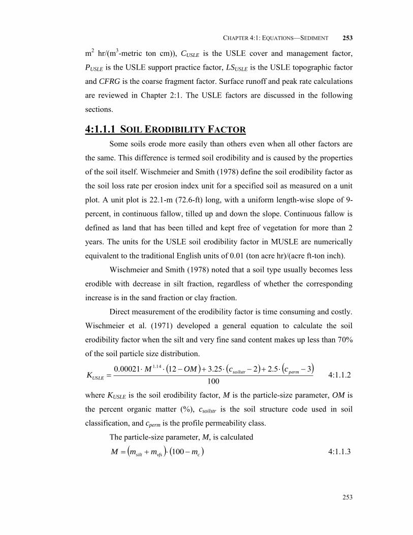
CHAPTER 4:1: EQUATIONS—SEDIMENT
253
253
m2 hr/(m3-metric ton cm)), CUSLE is the USLE cover and management factor,
PUSLE is the USLE support practice factor, LSUSLE is the USLE topographic factor
and CFRG is the coarse fragment factor. Surface runoff and peak rate calculations
are reviewed in Chapter 2:1. The USLE factors are discussed in the following
sections.
4:1.1.1 SOIL ERODIBILITY FACTOR Some soils erode more easily than others even when all other factors are
the same. This difference is termed soil erodibility and is caused by the properties
of the soil itself. Wischmeier and Smith (1978) define the soil erodibility factor as
the soil loss rate per erosion index unit for a specified soil as measured on a unit
plot. A unit plot is 22.1-m (72.6-ft) long, with a uniform length-wise slope of 9-
percent, in continuous fallow, tilled up and down the slope. Continuous fallow is
defined as land that has been tilled and kept free of vegetation for more than 2
years. The units for the USLE soil erodibility factor in MUSLE are numerically
equivalent to the traditional English units of 0.01 (ton acre hr)/(acre ft-ton inch).
Wischmeier and Smith (1978) noted that a soil type usually becomes less
erodible with decrease in silt fraction, regardless of whether the corresponding
increase is in the sand fraction or clay fraction.
Direct measurement of the erodibility factor is time consuming and costly.
Wischmeier et al. (1971) developed a general equation to calculate the soil
erodibility factor when the silt and very fine sand content makes up less than 70%
of the soil particle size distribution.
100
35.2225.31200021.0 14.1
permsoilstr
USLE
ccOMMK 4:1.1.2
where KUSLE is the soil erodibility factor, M is the particle-size parameter, OM is
the percent organic matter (%), csoilstr is the soil structure code used in soil
classification, and cperm is the profile permeability class.
The particle-size parameter, M, is calculated
cvfssilt mmmM 100 4:1.1.3

254 SWAT THEORETICAL DOCUMENTATION, VERSION 2009
254
where msilt is the percent silt content (0.002-0.05 mm diameter particles), mvfs is
the percent very fine sand content (0.05-0.10 mm diameter particles), and mc is
the percent clay content (< 0.002 mm diameter particles).
The percent organic matter content, OM, of a layer can be calculated:
orgCOM 72.1 4:1.1.4
where orgC is the percent organic carbon content of the layer (%).
Soil structure refers to the aggregation of primary soil particles into
compound particles which are separated from adjoining aggregates by surfaces of
weakness. An individual natural soil aggregate is called a ped. Field description of
soil structure notes the shape and arrangement of peds, the size of peds, and the
distinctness and durability of visible peds. USDA Soil Survey terminology for
structure consists of separate sets of terms defining each of these three qualities.
Shape and arrangement of peds are designated as type of soil structure; size of
peds as class; and degree of distinctness as grade.
The soil-structure codes for equation 4:1.1.2 are defined by the type and
class of soil structure present in the layer. There are four primary types of
structure:
-Platy, with particles arranged around a plane, generally horizontal
-Prismlike, with particles arranged around a verticle line and bounded by relatively flat vertical surfaces
-Blocklike or polyhedral, with particles arranged around a point and bounded by flat or rounded surfaces which are casts of the molds formed by the faces of surrounding peds
-Spheroidal or polyhedral, with particles arranged around a point and bounded by curved or very irregular surfaces that are not accomodated to the adjoining aggregates
Each of the last three types has two subtypes:
-Prismlike Prismatic: without rounded upper ends Columnar: with rounded caps
-Blocklike Angular Blocky: bounded by planes intersecting at relatively
sharp angles Subangular Blocky: having mixed rounded and plane faces
with vertices mostly rounded

CHAPTER 4:1: EQUATIONS—SEDIMENT
255
255
-Spheroidal Granular: relatively non-porous Crumb: very porous
The size criteria for the class will vary by type of structure and are
summarized in Table 4:1-1. The codes assigned to csoilstr are:
1 very fine granular 2 fine granular 3 medium or coarse granular 4 blocky, platy, prismlike or massive
Table 4:1-1: Size classes of soil structure Shape of structure Size Classes
Platy
Prismatic and Columnar
Blocky
Granular
Very fine < 1 mm < 10 mm < 5 mm < 1 mm Fine 1-2 mm 10-20 mm 5-10 mm 1-2 mm Medium 2-5 mm 20-50 mm 10-20 mm 2-5 mm Coarse 5-10 mm 50-100 mm 20-50 mm 5-10 mm Very coarse > 10 mm > 100 mm > 50 mm > 10 mm
Permeability is defined as the capacity of the soil to transmit water and air
through the most restricted horizon (layer) when moist. The profile permeability
classes are based on the lowest saturated hydraulic conductivity in the profile. The
codes assigned to cperm are:
1 rapid (> 150 mm/hr) 2 moderate to rapid (50-150 mm/hr) 3 moderate (15-50 mm/hr) 4 slow to moderate (5-15 mm/hr) 5 slow (1-5 mm/hr) 6 very slow (< 1 mm/hr)
Williams (1995) proposed an alternative equation:
hisandorgcsiclcsandUSLE ffffK 4:1.1.5
where fcsand is a factor that gives low soil erodibility factors for soils with high
coarse-sand contents and high values for soils with little sand, fcl-si is a factor that
gives low soil erodibility factors for soils with high clay to silt ratios, forgc is a
factor that reduces soil erodibility for soils with high organic carbon content, and
fhisand is a factor that reduces soil erodibility for soils with extremely high sand
contents. The factors are calculated:

256 SWAT THEORETICAL DOCUMENTATION, VERSION 2009
256
1001256.0exp3.02.0 silt
scsand
mmf 4:1.1.6
3.0
siltc
siltsicl
mm
mf 4:1.1.7
orgCorgC
orgCforgc 95.272.3exp
25.01 4:1.1.8
10019.2251.5exp
1001
10017.0
1ss
s
hisandmm
m
f 4:1.1.9
where ms is the percent sand content (0.05-2.00 mm diameter particles), msilt is the
percent silt content (0.002-0.05 mm diameter particles), mc is the percent clay
content (< 0.002 mm diameter particles), and orgC is the percent organic carbon
content of the layer (%).
4:1.1.2 COVER AND MANAGEMENT FACTOR The USLE cover and management factor, CUSLE, is defined as the ratio of
soil loss from land cropped under specified conditions to the corresponding loss
from clean-tilled, continuous fallow (Wischmeier and Smith, 1978). The plant
canopy affects erosion by reducing the effective rainfall energy of intercepted
raindrops. Water drops falling from the canopy may regain appreciable velocity
but it will be less than the terminal velocity of free-falling raindrops. The average
fall height of drops from the canopy and the density of the canopy will determine
the reduction in rainfall energy expended at the soil surface. A given percentage
of residue on the soil surface is more effective that the same percentage of canopy
cover. Residue intercepts falling raindrops so near the surface that drops regain no
fall velocity. Residue also obstructs runoff flow, reducing its velocity and
transport capacity.
Because plant cover varies during the growth cycle of the plant, SWAT
updates CUSLE daily using the equation:
mnUSLEsurfmnUSLEUSLE CrsdCC ,, ln00115.0expln8.0lnexp 4:1.1.10

CHAPTER 4:1: EQUATIONS—SEDIMENT
257
257
where CUSLE,mn is the minimum value for the cover and management factor for the
land cover, and rsdsurf is the amount of residue on the soil surface (kg/ha).
The minimum C factor can be estimated from a known average annual C
factor using the following equation (Arnold and Williams, 1995):
1034.0ln463.1 ,, aaUSLEmnUSLE CC 4:1.1.11
where CUSLE,mn is the minimum C factor for the land cover and CUSLE,aa is the
average annual C factor for the land cover.
4:1.1.3 SUPPORT PRACTICE FACTOR The support practice factor, PUSLE, is defined as the ratio of soil loss with a
specific support practice to the corresponding loss with up-and-down slope
culture. Support practices include contour tillage, stripcropping on the contour,
and terrace systems. Stabilized waterways for the disposal of excess rainfall are a
necessary part of each of these practices.
Contour tillage and planting provides almost complete protection against
erosion from storms of low to moderate intensity, but little or no protection
against occasional severe storms that cause extensive breakovers of contoured
rows. Contouring is most effective on slopes of 3 to 8 percent. Values for PUSLE
and slope-length limits for contour support practices are given in Table 4:1-2.
Table 4:1-2: P factor values and slope-length limits for contouring (Wischmeier and Smith, 1978).
Land slope (%) PUSLE Maximum length (m) 1 to 2 0.60 122 3 to 5 0.50 91 6 to 8 0.50 61
9 to 12 0.60 37 13 to 16 0.70 24 17 to 20 0.80 18 21 to 25 0.90 15
Stripcropping is a practice in which contoured strips of sod are alternated
with equal-width strips of row crop or small grain. Recommended values for
contour stripcropping are given in Table 4:1-3.

258 SWAT THEORETICAL DOCUMENTATION, VERSION 2009
258
Table 4:1-3: P factor values, maximum strip width and slope-length limits for contour stripcropping (Wischmeier and Smith, 1978).
Land slope (%)
PUSLE values1 Strip width (m)
Maximum length (m) A B C
1 to 2 0.30 0.45 0.60 40 244 3 to 5 0.25 0.38 0.50 30 183 6 to 8 0.25 0.38 0.50 30 122
9 to 12 0.30 0.45 0.60 24 73 13 to 16 0.35 0.52 0.70 24 49 17 to 20 0.40 0.60 0.80 18 37 21 to 25 0.45 0.68 0.90 15 30
1P values: A: For 4-year rotation of row crop, small grain with meadow seeding, and 2 years of meadow. A
second row crop can replace the small grain if meadow is established in it. B: For 4-year rotation of 2 years row crop, winter grain with meadow seeding, and 1-year meadow. C: For alternate strips of row crop and winter grain
Terraces are a series of horizontal ridges made in a hillside. There are
several types of terraces. Broadbase terraces are constructed on gently sloping
land and the channel and ridge are cropped the same as the interterrace area. The
steep backslope terrace, where the backslope is in sod, is most common on steeper
land. Impoundment terraces are terraces with underground outlets.
Terraces divide the slope of the hill into segments equal to the horizontal
terrace interval. With terracing, the slope length is the terrace interval. For
broadbase terraces, the horizontal terrace interval is the distance from the center
of the ridge to the center of the channel for the terrace below. The horizontal
terrace interval for steep backslope terraces is the distance from the point where
cultivation begins at the base of the ridge to the base of the frontslope of the
terrace below.
Values for PUSLE for contour farming terraced fields are listed in Table
4:1-4. These values apply to broadbase, steep backslope and level terraces. Keep
in mind that the values given in Table 4:1-4 do not account for all erosion control
benefits of terraces. The shorter slope-length used in the calculation of the length-
slope factor will produce additional reduction.

CHAPTER 4:1: EQUATIONS—SEDIMENT
259
259
Table 4:1-4: P factor values for contour-farmed terraced fields1 (from Wischmeier and Smith, 1978)
Land slope (%)
Farm planning Computing sediment yield3
Contour P factor2
Stripcrop P factor
Graded channels sod outlets
Steep backslope underground
outlets 1 to 2 0.60 0.30 0.12 0.05 3 to 8 0.50 0.25 0.10 0.05
9 to 12 0.60 0.30 0.12 0.05 13 to 16 0.70 0.35 0.14 0.05 17 to 20 0.80 0.40 0.16 0.06 21 to 25 0.90 0.45 0.18 0.06
1Slope length is the horizontal terrace interval. The listed values are for contour farming. No additional contouring factor is used in the computation.
2 Use these values for control of interterrace erosion within specified soil loss tolerances. 3 These values include entrapment efficiency and are used for control of offsite sediment within limits and for
estimating the field’s contribution to watershed sediment yield.
4:1.1.4 TOPOGRAPHIC FACTOR
The topographic factor, LSUSLE, is the expected ratio of soil loss per unit
area from a field slope to that from a 22.1-m length of uniform 9 percent slope
under otherwise identical conditions. The topographic factor is calculated:
065.0sin56.4sin41.651.22
2
hillhill
m
hillUSLE
LLS 4:1.1.12
where Lhill is the slope length (m), m is the exponential term, and hill is the angle
of the slope. The exponential term, m, is calculated:
slpm 835.35exp16.0 4:1.1.13
where slp is the slope of the HRU expressed as rise over run (m/m). The
relationship between hill and slp is:
hillslp tan 4:1.1.14
4:1.1.5 COARSE FRAGMENT FACTOR
The coarse fragment factor is calculated:
rockCFRG 053.0exp 4:1.1.15
where rock is the percent rock in the first soil layer (%).

260 SWAT THEORETICAL DOCUMENTATION, VERSION 2009
260
Table 4:1-5: SWAT input variables that pertain to sediment yield.
Variable Name
Definition Input File
USLE_K KUSLE: USLE soil erodibility factor (0.013 metric ton m2 hr/(m3-metric ton cm))
.sol
USLE_C CUSLE,mn: Minimum value for the cover and management factor for the land cover
crop.dat
USLE_P PUSLE: USLE support practice factor .mgt SLSUBBSN Lhill: Slope length (m) .hru HRU_SLP slp: Average slope of the subbasin (% or m/m) .hru ROCK rock: Percent rock in the first soil layer (%) .sol
4:1.2 USLE
For comparative purposes, SWAT prints out sediment loadings calculated
with USLE. These values are not used by the model, they are for comparison
only. The universal soil loss equation (Williams, 1995) is:
CFRGLSPCKEIsed USLEUSLEUSLEUSLEUSLE 292.1 4:1.2.1
where sed is the sediment yield on a given day (metric tons/ha), EIUSLE is the
rainfall erosion index (0.017 m-metric ton cm/(m2 hr)), KUSLE is the USLE soil
erodibility factor (0.013 metric ton m2 hr/(m3-metric ton cm)), CUSLE is the USLE
cover and management factor, PUSLE is the USLE support practice factor, LSUSLE
is the USLE topographic factor and CFRG is the coarse fragment factor. The
factors other than EIUSLE are discussed in the preceding sections.
4:1.2.1 RAINFALL ERODIBILITY INDEX The value of EIUSLE for a given rainstorm is the product, total storm energy
times the maximum 30 minute intensity. The storm energy indicates the volume
of rainfall and runoff while the 30 minute intensity indicates the prolonged peak
rates of detachment and runoff.
30IEEI stormUSLE 4:1.2.2
where EIUSLE is the rainfall erosion index (0.017 m-metric ton cm/(m2 hr)), Estorm
is the total storm energy (0.0017 m-metric ton/m2), and I30 is the maximum 30-
minute intensity (mm/hr).
The energy of a rainstorm is a function of the amount of rain and of all the
storm’s component intensities. Because rainfall is provided to the model in daily

CHAPTER 4:1: EQUATIONS—SEDIMENT
261
261
totals, an assumption must be made about variation in rainfall intensity. The
rainfall intensity variation with time is assumed to be exponentially distributed:
i
mxtk
tii exp 4:1.2.3
where it is the rainfall intensity at time t (mm/hr), imx is the maximum rainfall
intensity (mm/hr), t is the time (hr), and ki is the decay constant for rainfall
intensity (hr).
The USLE energy equation is
t
RRE
day
daystorm 10log9.81.12 4:1.2.4
where Rday is the amount of rainfall during the time interval (mm H2O), and t is
the time interval (hr). This equation may be expressed analytically as:
0
100
log9.81.12 dtiidtiE tttstorm 4:1.2.5
Combining equation 4:1.2.5 and 4:1.2.3 and integrating gives the equation
for estimating daily rainfall energy:
434.0log9.81.121000 10 mx
day
storm iR
E 4:1.2.6
where Rday is the amount of precipitation falling on a given day (mm H2O), and
imx is the maximum rainfall intensity (mm/hr). To compute the maximum rainfall
intensity, imx, equation 4:1.2.3 is integrated to give
imxday kiR 4:1.2.7
and
i
daytk
tRR exp1 4:1.2.8
where Rday is the amount of precipitation falling on a given day (mm H2O), imx is
the maximum rainfall intensity (mm/hr), ki is the decay constant for rainfall
intensity (hr), Rt is the amount of rain falling during a time interval (mm H2O),
and t is the time interval (hr). The maximum half-hour rainfall for the
precipitation event is known:

262 SWAT THEORETICAL DOCUMENTATION, VERSION 2009
262
dayRR 5.05.0 4:1.2.9
where R0.5 is the maximum half-hour rainfall (mm H2O), 0.5 is the maximum
half-hour rainfall expressed as a fraction of daily rainfall, and Rday is the amount
of precipitation falling on a given day (mm H2O). Calculation of 0.5 is reviewed
in Chapter 1:2 and Chapter 1:3. Substituting equation 4:1.2.9 and 4:1.2.7 into
4:1.2.8 and solving for the maximum intensity gives:
5.01ln2 daymx Ri 4:1.2.10
where imx is the maximum rainfall intensity (mm/hr), Rday is the amount of
precipitation falling on a given day (mm H2O), and 0.5 is the maximum half-hour
rainfall expressed as a fraction of daily rainfall.
The maximum 30 minute intensity is calculated:
dayRI 5.030 2 4:1.2.11
where I30 is the maximum 30-minute intensity (mm/hr), 0.5 is the maximum half-
hour rainfall expressed as a fraction of daily rainfall, and Rday is the amount of
precipitation falling on a given day (mm H2O).
Table 4:1-6: SWAT input variables that pertain to USLE sediment yield.
Variable Name
Definition Input File
USLE_K KUSLE: USLE soil erodibility factor (0.013 metric ton m2 hr/(m3-metric ton cm))
.sol
USLE_C CUSLE,mn: Minimum value for the cover and management factor for the land cover
crop.dat
USLE_P PUSLE: USLE support practice factor .mgt SLSUBBSN Lhill: Slope length (m) .hru SLOPE slp: Average slope of the subbasin (% or m/m) .hru ROCK rock: Percent rock in the first soil layer (%) .sol

CHAPTER 4:1: EQUATIONS—SEDIMENT
263
263
4:1.3 SNOW COVER EFFECTS The erosive power of rain and runoff will be less when snow cover is
present than when there is no snow cover. During periods when snow is present in
an HRU, SWAT modifies the sediment yield using the following relationship:
4.253exp SNO
dsesed 4:1.3.1
where sed is the sediment yield on a given day (metric tons), dse is the sediment
yield calculated with MUSLE (metric tons), and SNO is the water content of the
snow cover (mm H2O).
4:1.4 SEDIMENT LAG IN SURFACE RUNOFF In large subbasins with a time of concentration greater than 1 day, only a
portion of the surface runoff will reach the main channel on the day it is
generated. SWAT incorporates a surface runoff storage feature to lag a portion of
the surface runoff release to the main channel. Sediment in the surface runoff is
lagged as well.
Once the sediment load in surface runoff is calculated, the amount of
sediment released to the main channel is calculated:
conc
istort
surlagseddsesed exp11, 4:1.4.1
where sed is the amount of sediment discharged to the main channel on a given
day (metric tons), dse is the amount of sediment load generated in the HRU on a
given day (metric tons), sedstor,i-1 is the sediment stored or lagged from the
previous day (metric tons), surlag is the surface runoff lag coefficient, and tconc is
the time of concentration for the HRU (hrs).

264 SWAT THEORETICAL DOCUMENTATION, VERSION 2009
264
The expression
conct
surlagexp1 in equation 4:1.4.1 represents the
fraction of the total available sediment that will be allowed to enter the reach on
any one day. Figure 4:1-1 plots values for this expression at different values for
surlag and tconc.
Figure 4:1-1: Influence of surlag and tconc on fraction of surface runoff and sediment released.
Note that for a given time of concentration, as surlag decreases in value
more sediment is held in storage.
Table 4:1-7: SWAT input variables that pertain to sediment lag calculations.
Variable Name
Definition Input File
SURLAG surlag: surface runoff lag coefficient .bsn
4:1.5 SEDIMENT IN LATERAL & GROUNDWATER FLOW
SWAT allows the lateral and groundwater flow to contribute sediment to
the main channel. The amount of sediment contributed by lateral and groundwater
flow is calculated:
1000sedhrugwlat
lat
concareaQQsed
4:1.5.1
where sedlat is the sediment loading in lateral and groundwater flow (metric tons),
Qlat is the lateral flow for a given day (mm H2O), Qgw is the groundwater flow for

CHAPTER 4:1: EQUATIONS—SEDIMENT
265
265
a given day (mm H2O), areahru is the area of the HRU (km2), and concsed is the
concentration of sediment in lateral and groundwater flow (mg/L).
Table 4:1-8: SWAT input variables that pertain to sediment lag calculations.
Variable Name
Definition Input File
LAT_SED concsed: Concentration of sediment in lateral and groundwater flow (mg/L)
.hru
4:1.6 NOMENCLATURE CUSLE USLE cover and management factor CUSLE,aa Average annual C factor for the land cover CUSLE,mn Minimum value for the cover and management factor for the land cover CFRG Coarse fragment factor Estorm Total storm energy (0.0017 m-metric ton/m2), EIUSLE Rainfall erosion index (0.017 m-metric ton cm/(m2 hr)) I30 Maximum 30 minute intensity (mm/hr) KUSLE USLE soil erodibility factor (0.013 metric ton m2 hr/(m3-metric ton cm)) Lhill Slope length (m) LSUSLE USLE topographic factor M Particle-size parameter for estimation of USLE K factor OM Percent organic matter (%) PUSLE USLE support practice factor Qgw Groundwater flow for a given day (mm H2O) Qlat Lateral flow (mm H2O) Qsurf Surface runoff volume (mm H2O/ha) Rday Amount of rainfall on a given day (mm H2O) SNO Water content of the snow cover (mm H2O)
areahru HRU area (ha or km2) cperm Profile-permeability class
csoilstr Soil-structure code used in soil classification concsed Concentration of sediment in lateral and groundwater flow (mg/L) fcl-si Factor that gives low soil erodibility factors for soils with high clay to silt ratios fcsand Factor that gives low soil erodibility factors for soils with high coarse-sand
contents and high values for soils with little sand fhisand Factor that reduces soil erodibility for soils with extremely high sand contents
forgc Factor that reduces soil erodibility for soils with high organic carbon content imx Maximum rainfall intensity (mm/hr) it Rainfall intensity at time t (mm/hr) ki Decay constant for rainfall intensity (hr) m Exponential term in USLE LS factor calculation mc Percent clay content (< 0.002 mm diameter particles) ms Percent sand content

266 SWAT THEORETICAL DOCUMENTATION, VERSION 2009
266
msilt Percent silt content (0.002-0.05 mm diameter particles) mvfs Percent very fine sand content (0.05-0.10 mm diameter particles) orgCly Amount of organic carbon in the layer (%) qpeak Peak runoff rate (m3/s) rock Percent rock in soil layer (%) rsdsurf Amount of residue on the soil surface (kg/ha) sed Sediment yield on a given day (metric tons) sedlat Sediment loading in lateral and groundwater flow (metric tons) sedstor,i-1 Sediment stored or lagged from the previous day (metric tons) slp Average slope of the subbasin (m/m) surlag Surface runoff lag coefficient t Time (hr) tconc Time of concentration for a subbasin (hr) 0.5 Maximum half-hour rainfall expressed as a fraction of daily rainfall hill Angle of the slope
4:1.7 REFERENCES
Arnold, J.G. and J.R. Williams. 1995. SWRRB—A watershed scale model for soil and water resources management. p. 847-908. In V.P. Singh (ed) Computer models of watershed hydrology. Water Resources Publications.
Williams, J.R. 1975. Sediment-yield prediction with universal equation using runoff energy factor. p. 244-252. In Present and prospective technology for predicting sediment yield and sources: Proceedings of the sediment-yield workshop, USDA Sedimentation Lab., Oxford, MS, November 28-30, 1972. ARS-S-40.
Williams, J.R. 1995. Chapter 25: The EPIC model. p. 909-1000. In V.P. Singh (ed.) Computer models of watershed hydrology. Water Resources Publications.
Wischmeier, W.H., C.B. Johnson, and B.V. Cross. 1971. A soil erodibility nomograph for farmland and construction sites. Journal of Soil and Water Conservation 26:189-193.
Wischmeier, W.H. and D.D. Smith. 1965. Predicting rainfall-erosion losses from cropland east of the Rocky Mountains. Agriculture Handbook 282. USDA-ARS
Wischmeier, W.H. and D.D. Smith. 1978. Predicting rainfall erosion losses: a guide to conservation planning. Agriculture Handbook 282. USDA-ARS

CHAPTER 4:1: EQUATIONS—SEDIMENT
267
267
268
SECTION 4 CHAPTER 2
EQUATIONS:
NUTRIENT TRANSPORT
The transport of nutrients from land areas into streams and water bodies is
a normal result of soil weathering and erosion processes. However, excessive
loading of nutrients into streams and water bodies will accelerate eutrophication
and render the water unfit for human consumption. This chapter reviews the
algorithms governing movement of mineral and organic forms of nitrogen and
phosphorus from land areas to the stream network.

CHAPTER 4:2: EQUATIONS—NUTRIENT TRANSPORT
269
269
4:2.1 NITRATE MOVEMENT
Most soil minerals are negatively charged at normal pH and the net
interaction with anions such as nitrate is a repulsion from particle surfaces. This
repulsion is termed negative adsorption or anion exclusion.
Anions are excluded from the area immediately adjacent to mineral
surfaces due to preferential attraction of cations to these sites. This process has a
direct impact on the transport of anions through the soil for it effectively excludes
anions from the slowest moving portion of the soil water volume found closest to
the charged particle surfaces (Jury et al, 1991). In effect, the net pathway of the
anion through the soil is shorter than it would be if all the soil water had to be
used (Thomas and McMahon, 1972).
Nitrate may be transported with surface runoff, lateral flow or percolation.
To calculate the amount of nitrate moved with the water, the concentration of
nitrate in the mobile water is calculated. This concentration is then multiplied by
the volume of water moving in each pathway to obtain the mass of nitrate lost
from the soil layer.
The concentration of nitrate in the mobile water fraction is calculated:
mobile
lye
mobilely
mobileNOw
SAT
wNO3
conc
1
exp1
,3 4:2.1.2
where concNO3,mobile is the concentration of nitrate in the mobile water for a given
layer (kg N/mm H2O), NO3ly is the amount of nitrate in the layer (kg N/ha), wmobile
is the amount of mobile water in the layer (mm H2O), e is the fraction of porosity
from which anions are excluded, and SATly is the saturated water content of the
soil layer (mm H2O). The amount of mobile water in the layer is the amount of
water lost by surface runoff, lateral flow or percolation:
lyperclylatsurfmobile wQQw ,, for top 10 mm 4:2.1.3
lyperclylatmobile wQw ,, for lower soil layers 4:2.1.4
where wmobile is the amount of mobile water in the layer (mm H2O), Qsurf is the
surface runoff generated on a given day (mm H2O), Qlat,ly is the water discharged

270 SWAT THEORETICAL DOCUMENTATION, VERSION 2009
270
from the layer by lateral flow (mm H2O), and wperc,ly is the amount of water
percolating to the underlying soil layer on a given day (mm H2O). Surface runoff
is allowed to interact with and transport nutrients from the top 10 mm of soil.
Nitrate removed in surface runoff is calculated:
surfmobileNONOsurf QconcNO3 ,33 4:2.1.5
where NO3surf is the nitrate removed in surface runoff (kg N/ha), NO3 is the
nitrate percolation coefficient, concNO3,mobile is the concentration of nitrate in the
mobile water for the top 10 mm of soil (kg N/mm H2O), and Qsurf is the surface
runoff generated on a given day (mm H2O). The nitrate percolation coefficient
allows the user to set the concentration of nitrate in surface runoff to a fraction of
the concentration in percolate.
Nitrate removed in lateral flow is calculated:
lylatmobileNONOlylat QconcNO3 ,,33, for top 10 mm 4:2.1.6
lylatmobileNOlylat QconcNO3 ,,3, for lower layers 4:2.1.7
where NO3lat,ly is the nitrate removed in lateral flow from a layer (kg N/ha), NO3
is the nitrate percolation coefficient, concNO3,mobile is the concentration of nitrate in
the mobile water for the layer (kg N/mm H2O), and Qlat,ly is the water discharged
from the layer by lateral flow (mm H2O).
Nitrate moved to the underlying layer by percolation is calculated:
lypercmobileNOlyperc wconcNO3 ,,3, 4:2.1.8
where NO3perc,ly is the nitrate moved to the underlying layer by percolation (kg
N/ha), concNO3,mobile is the concentration of nitrate in the mobile water for the
layer (kg N/mm H2O), and wperc,ly is the amount of water percolating to the
underlying soil layer on a given day (mm H2O).
Table 4:2-1: SWAT input variables that pertain to nitrate transport.
Variable Name
Definition Input File
ANION_EXCL e: Fraction of porosity from which anions are excluded .sol NPERCO NO3: Nitrate percolation coefficient .bsn

CHAPTER 4:2: EQUATIONS—NUTRIENT TRANSPORT
271
271
4:2.2 ORGANIC N IN SURFACE RUNOFF Organic N attached to soil particles may be transported by surface runoff
to the main channel. This form of nitrogen is associated with the sediment loading
from the HRU and changes in sediment loading will be reflected in the organic
nitrogen loading. The amount of organic nitrogen transported with sediment to the
stream is calculated with a loading function developed by McElroy et al. (1976)
and modified by Williams and Hann (1978).
sedN
hru
orgNsurfarea
sedconcorgN :001.0 4:2.2.1
where orgNsurf is the amount of organic nitrogen transported to the main channel
in surface runoff (kg N/ha), concorgN is the concentration of organic nitrogen in
the top 10 mm (g N/ metric ton soil), sed is the sediment yield on a given day
(metric tons), areahru is the HRU area (ha), and N:sed is the nitrogen enrichment
ratio.
The concentration of organic nitrogen in the soil surface layer, concorgN, is
calculated:
surfb
surfactsurfstasurffrsh
orgNdepth
orgNorgNorgNconc
,,,100 4:2.2.2
where orgNfrsh,surf is nitrogen in the fresh organic pool in the top 10mm (kg N/ha),
orgNsta,surf is nitrogen in the stable organic pool (kg N/ha), orgNact,surf is nitrogen
in the active organic pool in the top 10 mm (kg N/ha), b is the bulk density of the
first soil layer (Mg/m3), and depthsurf is the depth of the soil surface layer (10
mm).
4:2.2.1 ENRICHMENT RATIO As surface runoff flows over the soil surface, part of the water’s energy is
used to pick up and transport soil particles. The smaller particles weigh less and
are more easily transported than coarser particles. When the particle size
distribution of the transported sediment is compared to that of the soil surface
layer, the sediment load to the main channel has a greater proportion of clay sized
particles. In other words, the sediment load is enriched in clay particles. Organic

272 SWAT THEORETICAL DOCUMENTATION, VERSION 2009
272
nitrogen in the soil is attached primarily to colloidal (clay) particles, so the
sediment load will also contain a greater proportion or concentration of organic N
than that found in the soil surface layer.
The enrichment ratio is defined as the ratio of the concentration of organic
nitrogen transported with the sediment to the concentration in the soil surface
layer. SWAT will calculate an enrichment ratio for each storm event, or allow the
user to define a particular enrichment ratio for organic nitrogen that is used for all
storms during the simulation. To calculate the enrichment ratio, SWAT uses a
relationship described by Menzel (1980) in which the enrichment ratio is
logarithmically related to sediment concentration. The equation used to calculate
the nitrogen enrichment ratio, N:sed, for each storm event is:
2468.0,: 78.0
surqsedsedN conc 4:2.2.3
where concsed,surq is the concentration of sediment in surface runoff (Mg sed/m3
H2O). The concentration of sediment in surface runoff is calculated:
surfhru
surqsedQarea
sedconc
10, 4:2.2.4
where sed is the sediment yield on a given day (metric tons), areahru is the HRU
area (ha), and Q,surf is the amount of surface runoff on a given day (mm H2O).
Table 4:2-2: SWAT input variables that pertain to organic N loading.
Variable Name
Definition Input File
SOL_BD b: Bulk density (Mg/m3) .sol ERORGN N:sed: Organic nitrogen enrichment ratio .hru
4:2.3 SOLUBLE PHOSPHORUS MOVEMENT The primary mechanism of phosphorus movement in the soil is by
diffusion. Diffusion is the migration of ions over small distances (1-2 mm) in the
soil solution in response to a concentration gradient. Due to the low mobility of
solution phosphorus, surface runoff will only partially interact with the solution P
stored in the top 10 mm of soil. The amount of solution P transported in surface
runoff is:

CHAPTER 4:2: EQUATIONS—NUTRIENT TRANSPORT
273
273
surfdsurfb
surfsurfsolution
surfkdepth
QPP
,
,
4:2.3.1
where Psurf is the amount of soluble phosphorus lost in surface runoff (kg P/ha),
Psolution,surf is the amount of phosphorus in solution in the top 10 mm (kg P/ha),
Q,surf is the amount of surface runoff on a given day (mm H2O), b is the bulk
density of the top 10 mm (Mg/m3) (assumed to be equivalent to bulk density of
first soil layer), depthsurf is the depth of the “surface” layer (10 mm), and kd,surf is
the phosphorus soil partitioning coefficient (m3/Mg). The phosphorus soil
partitioning coefficient is the ratio of the soluble phosphorus concentration in the
surface 10 mm of soil to the concentration of soluble phosphorus in surface
runoff.
Table 4:2-3: SWAT input variables that pertain to soluble P runoff.
Variable Name
Definition Input File
SOL_BD b: Bulk density (Mg/m3) .sol PHOSKD kd,surf: Phosphorus soil partitioning coefficient (m3/Mg) .bsn
4:2.4 ORGANIC & MINERAL P ATTACHED TO SEDIMENT IN SURFACE RUNOFF
Organic and mineral P attached to soil particles may be transported by
surface runoff to the main channel. This form of phosphorus is associated with the
sediment loading from the HRU and changes in sediment loading will be reflected
in the loading of these forms of phosphorus. The amount of phosphorus
transported with sediment to the stream is calculated with a loading function
developed by McElroy et al. (1976) and modified by Williams and Hann (1978).
sedP
hru
sedPsurfarea
sedconcsedP :001.0 4:2.4.1
where sedPsurf is the amount of phosphorus transported with sediment to the main
channel in surface runoff (kg P/ha), concsedP is the concentration of phosphorus
attached to sediment in the top 10 mm (g P/ metric ton soil), sed is the sediment
yield on a given day (metric tons), areahru is the HRU area (ha), and P:sed is the
phosphorus enrichment ratio.

274 SWAT THEORETICAL DOCUMENTATION, VERSION 2009
274
The concentration of phosphorus attached to sediment in the soil surface
layer, concsedP, is calculated:
surfb
surffrshsurfhumsurfstasurfact
sedPdepth
orgPorgPminPminPconc
,,,,100 4:2.4.2
where minPact,surf is the amount of phosphorus in the active mineral pool in the top
10 mm (kg P/ha), minPsta,surf is the amount of phosphorus in the stable mineral
pool in the top 10 mm (kg P/ha), orgPhum,surf is the amount of phosphorus in
humic organic pool in the top 10 mm (kg P/ha), orgPfrsh,surf is the amount of
phosphorus in the fresh organic pool in the top 10 mm (kg P/ha), b is the bulk
density of the first soil layer (Mg/m3), and depthsurf is the depth of the soil surface
layer (10 mm).
4:2.4.1 ENRICHMENT RATIO The enrichment ratio is defined as the ratio of the concentration of
phosphorus transported with the sediment to the concentration of phosphorus in
the soil surface layer. SWAT will calculate an enrichment ratio for each storm
event, or allow the user to define a particular enrichment ratio for phosphorus
attached to sediment that is used for all storms during the simulation. To calculate
the enrichment ratio, SWAT uses a relationship described by Menzel (1980) in
which the enrichment ratio is logarithmically related to sediment concentration.
The equation used to calculate the phosphorus enrichment ratio, P:sed, for each
storm event is:
2468.0,: 78.0
surqsedsedP conc 4:2.4.3
where concsed,surq is the concentration of sediment in surface runoff (Mg sed/m3
H2O). The concentration of sediment in surface runoff is calculated:
surfhru
surqsedQarea
sedconc
10, 4:2.4.4
where sed is the sediment yield on a given day (metric tons), areahru is the HRU
area (ha), and Qsurf is the amount of surface runoff on a given day (mm H2O).
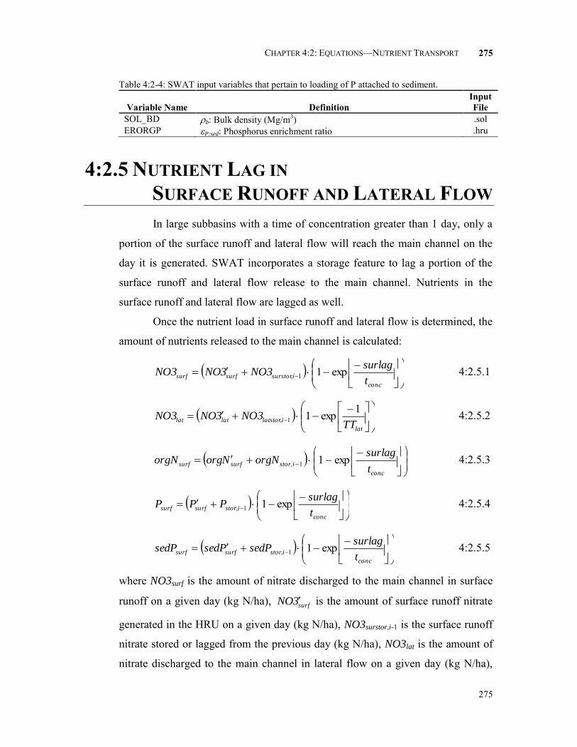
CHAPTER 4:2: EQUATIONS—NUTRIENT TRANSPORT
275
275
Table 4:2-4: SWAT input variables that pertain to loading of P attached to sediment.
Variable Name
Definition Input File
SOL_BD b: Bulk density (Mg/m3) .sol ERORGP P:sed: Phosphorus enrichment ratio .hru
4:2.5 NUTRIENT LAG IN SURFACE RUNOFF AND LATERAL FLOW
In large subbasins with a time of concentration greater than 1 day, only a
portion of the surface runoff and lateral flow will reach the main channel on the
day it is generated. SWAT incorporates a storage feature to lag a portion of the
surface runoff and lateral flow release to the main channel. Nutrients in the
surface runoff and lateral flow are lagged as well.
Once the nutrient load in surface runoff and lateral flow is determined, the
amount of nutrients released to the main channel is calculated:
conc
isurstorsurfsurft
surlagNO33NONO3 exp11, 4:2.5.1
lat
ilatstorlatlatTT
NO33NONO31exp11, 4:2.5.2
conc
istorsurfsurft
surlagorgNNorgorgN exp11, 4:2.5.3
conc
istorsurfsurft
surlagPPP exp11, 4:2.5.4
conc
istorsurfsurft
surlagsedPPsedsedP exp11, 4:2.5.5
where NO3surf is the amount of nitrate discharged to the main channel in surface
runoff on a given day (kg N/ha), surf3NO is the amount of surface runoff nitrate
generated in the HRU on a given day (kg N/ha), NO3surstor,i-1 is the surface runoff
nitrate stored or lagged from the previous day (kg N/ha), NO3lat is the amount of
nitrate discharged to the main channel in lateral flow on a given day (kg N/ha),

276 SWAT THEORETICAL DOCUMENTATION, VERSION 2009
276
lat3NO is the amount of lateral flow nitrate generated in the HRU on a given day
(kg N/ha), NO3latstor,i-1 is the lateral flow nitrate stored or lagged from the previous
day (kg N/ha), orgNsurf is the amount of organic N discharged to the main channel
in surface runoff on a given day (kg N/ha), surfNorg is the organic N loading
generated in the HRU on a given day (kg N/ha), orgNstor,i-1 is the organic N stored
or lagged from the previous day (kg N/ha), Psurf is the amount of solution P
discharged to the main channel in surface runoff on a given day (kg P/ha), surfP is
the amount of solution P loading generated in the HRU on a given day (kg P/ha),
Pstor,i-1 is the solution P loading stored or lagged from the previous day (kg P/ha),
sedPsurf is the amount of sediment-attached P discharged to the main channel in
surface runoff on a given day (kg P/ha), surfPsed is the amount of sediment-
attached P loading generated in the HRU on a given day (kg P/ha), sedPstor,i-1 is
the sediment-attached P stored or lagged from the previous day (kg P/ha), surlag
is the surface runoff lag coefficient, tconc is the time of concentration for the HRU
(hrs) and TTlag is the lateral flow travel time (days).
Table 4:2-5: SWAT input variables that pertain to nutrient lag calculations.
Variable Name
Definition Input File
SURLAG surlag: surface runoff lag coefficient .bsn LAT_TTIME TTlag: Lateral flow travel time (days) .hru
4:2.6 NOMENCLATURE NO3lat,ly Nitrate removed in lateral flow from a layer (kg N/ha)
lat3NO Amount of lateral flow nitrate generated in HRU on a given day (kg N/ha) NO3latstor,i-1 Lateral flow nitrate stored or lagged from the previous day (kg N/ha) NO3ly Amount of nitrate in the layer (kg N/ha) NO3perc,ly Nitrate moved to the underlying layer by percolation (kg N/ha) NO3surf Nitrate removed in surface runoff (kg N/ha)
surf3NO Amount of surface runoff nitrate generated in HRU on a given day (kg N/ha) NO3surstor,i-1 Surface runoff nitrate stored or lagged from the previous day (kg N/ha) Psolution,surf Amount of phosphorus in solution in the top 10 mm (kg P/ha) Pstor,i-1 Solution P loading stored or lagged from the previous day (kg P/ha) Psurf Amount of soluble phosphorus lost in surface runoff (kg P/ha)
surfP Amount of solution P loading generated in HRU on a given day (kg P/ha)
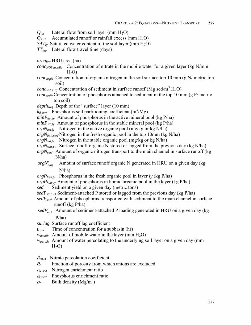
CHAPTER 4:2: EQUATIONS—NUTRIENT TRANSPORT
277
277
Qlat Lateral flow from soil layer (mm H2O) Qsurf Accumulated runoff or rainfall excess (mm H2O) SATly Saturated water content of the soil layer (mm H2O) TTlag Lateral flow travel time (days)
areahru HRU area (ha) concNO3,mobile Concentration of nitrate in the mobile water for a given layer (kg N/mm
H2O) concorgN Concentration of organic nitrogen in the soil surface top 10 mm (g N/ metric ton
soil) concsed,surq Concentration of sediment in surface runoff (Mg sed/m3 H2O) concsedP Concentration of phosphorus attached to sediment in the top 10 mm (g P/ metric
ton soil) depthsurf Depth of the “surface” layer (10 mm) kd,surf Phosphorus soil partitioning coefficient (m3/Mg) minPact,ly Amount of phosphorus in the active mineral pool (kg P/ha) minPsta,ly Amount of phosphorus in the stable mineral pool (kg P/ha) orgNact,ly Nitrogen in the active organic pool (mg/kg or kg N/ha) orgNfrsh,surf Nitrogen in the fresh organic pool in the top 10mm (kg N/ha) orgNsta,ly Nitrogen in the stable organic pool (mg/kg or kg N/ha) orgNstor,i-1 Surface runoff organic N stored or lagged from the previous day (kg N/ha) orgNsurf Amount of organic nitrogen transport to the main channel in surface runoff (kg
N/ha) surfNorg Amount of surface runoff organic N generated in HRU on a given day (kg
N/ha) orgPfrsh,ly Phosphorus in the fresh organic pool in layer ly (kg P/ha) orgPhum,ly Amount of phosphorus in humic organic pool in the layer (kg P/ha) sed Sediment yield on a given day (metric tons) sedPstor,i-1 Sediment-attached P stored or lagged from the previous day (kg P/ha) sedPsurf Amount of phosphorus transported with sediment to the main channel in surface
runoff (kg P/ha) surfPsed Amount of sediment-attached P loading generated in HRU on a given day (kg
P/ha) surlag Surface runoff lag coefficient tconc Time of concentration for a subbasin (hr) wmobile Amount of mobile water in the layer (mm H2O) wperc,ly Amount of water percolating to the underlying soil layer on a given day (mm
H2O)
NO3 Nitrate percolation coefficient e Fraction of porosity from which anions are excluded
N:sed Nitrogen enrichment ratio
P:sed Phosphorus enrichment ratio
b Bulk density (Mg/m3)

278 SWAT THEORETICAL DOCUMENTATION, VERSION 2009
278
4:2.7 REFERENCES
Jury, W.A., W.R. Gardner, and W.H. Gardner. 1991. Soil physics, 5th edition.
John Wiley & Sons, Inc. New York, N.Y.
McElroy, A.D., S.Y. Chiu, J.W. Nebgen, A. Aleti, and F.W. Bennett. 1976.
Loading functions for assessment of water pollution from nonpoint
sources. Environ. Prot. Tech. Serv., EPA 600/2-76-151.
Menzel, R.G. 1980. Enrichment ratios for water quality modeling. p. 486-492. In
W.G. Knisel (ed.) CREAMS, A field scale model for chemicals, runoff,
and erosion from agricultural management systems. U.S. Dept. Agric.
Conserv. Res. Rept. No. 26.
Thomas, G.W. and M. McMahon. 1972. The relation between soil characteristics,
water movement and nitrate concentration of ground water. Univ. of
Kentucky Water Resources Institute Research Report No. 52, Lexington,
KY.
Williams, J.R. and R.W. Hann. 1978. Optimal operation of large agricultural
watersheds with water quality constraints. Texas Water Resources
Institute, Texas A&M Univ., Tech. Rept. No. 96.

CHAPTER 4:2: EQUATIONS—NUTRIENT TRANSPORT
279
279

280
SECTION 4 CHAPTER 3
EQUATIONS:
PESTICIDE TRANSPORT
The transport of pesticide from land areas into streams and water bodies is
a result of soil weathering and erosion processes. Excessive loading of pesticides
in streams and water bodies can produce toxic conditions that harm aquatic life
and render the water unfit for human consumption. This chapter reviews the
algorithms governing movement of soluble and sorbed forms of pesticide from
land areas to the stream network. Pesticide transport algorithms in SWAT were
taken from EPIC (Williams, 1995).

CHAPTER 4:3: EQUATIONS—PESTICIDE TRANSPORT
281
281
4:3.1 PHASE DISTRIBUTION OF PESTICIDE Pesticide in the soil environment can be transported in solution or attached
to sediment. The partitioning of a pesticide between the solution and soil phases is
defined by the soil adsorption coefficient for the pesticide. The soil adsorption
coefficient is the ratio of the pesticide concentration in the soil or solid phase to
the pesticide concentration in the solution or liquid phase:
solution
solidphase
pC
CK 4:3.1.1
where Kp is the soil adsorption coefficient ((mg/kg)/(mg/L) or m3/ton), Csolidphase is
the concentration of the pesticide sorbed to the solid phase (mg chemical/kg solid
material or g/ton), and Csolution is the concentration of the pesticide in solution (mg
chemical/L solution or g/ton). The definition of the soil adsorption coefficient in
equation 4:3.1.1 assumes that the pesticide sorption process is linear with
concentration and instantaneously reversible.
Because the partitioning of pesticide is dependent upon the amount of
organic material in the soil, the soil adsorption coefficient input to the model is
normalized for soil organic carbon content. The relationship between the soil
adsorption coefficient and the soil adsorption coefficient normalized for soil
organic carbon content is:
100orgC
KK ocp 4:3.1.2
where Kp is the soil adsorption coefficient ((mg/kg)/(mg/L)), Koc is the soil
adsorption coefficient normalized for soil organic carbon content ((mg/kg)/(mg/L)
or m3/ton), and orgC is the percent organic carbon present in the soil.
Table 4:3-1: SWAT input variables that pertain to pesticide phase partitioning.
Variable Name
Definition Input File
SOL_CBN orgCly: Amount of organic carbon in the layer (%) .sol SKOC Koc: Soil adsorption coefficient normalized for soil organic
carbon content (ml/g or (mg/kg)/(mg/L) or L/kg) pest.dat

282 SWAT THEORETICAL DOCUMENTATION, VERSION 2009
282
4:3.2 MOVEMENT OF SOLUBLE PESTICIDE
Pesticide in the soluble phase may be transported with surface runoff,
lateral flow or percolation. The change in the amount of pesticide contained in a
soil layer due to transport in solution with flow is a function of time,
concentration and amount of flow:
mobilesolution
lyswC
dt
dpst 01.0, 4:3.2.1
where psts,ly is the amount of pesticide in the soil layer (kg pst/ha), Csolution is the
pesticide concentration in solution (mg/L or g/ton), and wmobile is the amount of
mobile water on a given day (mm H2O). The amount of mobile water in the layer
is the amount of water lost by surface runoff, lateral flow or percolation:
surfpercsurflatsurfmobile wQQw ,, for top 10 mm 4:3.2.2
lyperclylatmobile wQw ,, for lower soil layers 4:3.2.3
where wmobile is the amount of mobile water in the layer (mm H2O), Qsurf is the
surface runoff generated on a given day (mm H2O), Qlat,ly is the water discharged
from the layer by lateral flow (mm H2O), and wperc,ly is the amount of water
percolating to the underlying soil layer on a given day (mm H2O).
The total amount of pesticide in the soil layer is the sum of the adsorbed
and dissolved phases:
lybsolidphaselysolutionlys depthCSATCpst 01.0, 4:3.2.4
where psts,ly is the amount of pesticide in the soil layer (kg pst/ha), Csolution is the
pesticide concentration in solution (mg/L or g/ton), SATly is the amount of water
in the soil layer at saturation (mm H2O), Csolidphase is the concentration of the
pesticide sorbed to the solid phase (mg/kg or g/ton), b is the bulk density of the
soil layer (Mg/m3), and depthly is the depth of the soil layer (mm). Rearranging
equation 4:3.1.1 to solve for Csolidphase and substituting into equation 4:3.2.4
yields:
lybpsolutionlysolutionlys depthKCSATCpst 01.0, 4:3.2.5
which rearranges to
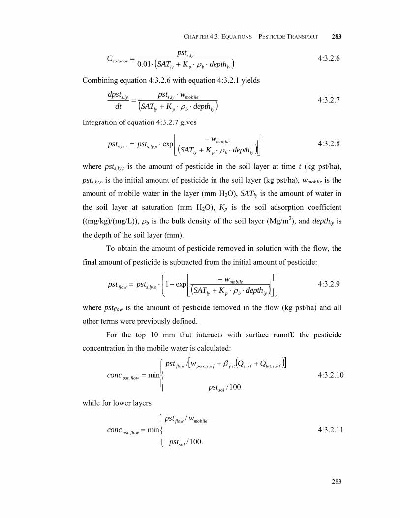
CHAPTER 4:3: EQUATIONS—PESTICIDE TRANSPORT
283
283
lybply
lys
solutiondepthKSAT
pstC
01.0, 4:3.2.6
Combining equation 4:3.2.6 with equation 4:3.2.1 yields
lybply
mobilelyslys
depthKSAT
wpst
dt
dpst
,, 4:3.2.7
Integration of equation 4:3.2.7 gives
lybply
mobileolystlys
depthKSAT
wpstpst
exp,,,, 4:3.2.8
where psts,ly,t is the amount of pesticide in the soil layer at time t (kg pst/ha),
psts,ly,o is the initial amount of pesticide in the soil layer (kg pst/ha), wmobile is the
amount of mobile water in the layer (mm H2O), SATly is the amount of water in
the soil layer at saturation (mm H2O), Kp is the soil adsorption coefficient
((mg/kg)/(mg/L)), b is the bulk density of the soil layer (Mg/m3), and depthly is
the depth of the soil layer (mm).
To obtain the amount of pesticide removed in solution with the flow, the
final amount of pesticide is subtracted from the initial amount of pesticide:
lybply
mobileolysflow
depthKSAT
wpstpst
exp1,, 4:3.2.9
where pstflow is the amount of pesticide removed in the flow (kg pst/ha) and all
other terms were previously defined.
For the top 10 mm that interacts with surface runoff, the pesticide
concentration in the mobile water is calculated:
.100/
/min
,,
,
sol
surflatsurfpstsurfpercflow
flowpst
pst
QQwpst
conc
4:3.2.10
while for lower layers
.100/
/min,
sol
mobileflow
flowpst
pst
wpst
conc 4:3.2.11

284 SWAT THEORETICAL DOCUMENTATION, VERSION 2009
284
where concpst,flow is the concentration of pesticide in the mobile water (kg pst/ha-
mm H2O), pstflow is the amount of pesticide removed in the flow (kg pst/ha), pst is
the pesticide percolation coefficient, Qsurf is the surface runoff generated on a
given day (mm H2O), Qlat,ly is the water discharged from the layer by lateral flow
(mm H2O), wperc,ly is the amount of water percolating to the underlying soil layer
on a given day (mm H2O), wmobile is the amount of mobile water in the layer (mm
H2O), and pstsol is the solubility of the pesticide in water (mg/L).
Pesticide moved to the underlying layer by percolation is calculated:
lypercflowpstlyperc wconcpst ,,, 4:3.2.12
where pstperc,ly is the pesticide moved to the underlying layer by percolation (kg
pst/ha), concpst,flow is the concentration of pesticide in the mobile water for the
layer (kg pst/mm H2O), and wperc,ly is the amount of water percolating to the
underlying soil layer on a given day (mm H2O).
Pesticide removed in lateral flow is calculated:
surflatflowpstpstsurflat Qconcpst ,,, for top 10 mm 4:3.2.13
lylatflowpstlylat Qconcpst ,,, for lower layers 4:3.2.14
where pstlat,ly is the pesticide removed in lateral flow from a layer (kg pst/ha), pst
is the pesticide percolation coefficient, concpst,flow is the concentration of pesticide
in the mobile water for the layer (kg pst/mm H2O), and Qlat,ly is the water
discharged from the layer by lateral flow (mm H2O). The pesticide percolation
coefficient allows the user to set the concentration of pesticide in runoff and
lateral flow from the top 10 mm to a fraction of the concentration in percolate.
Pesticide removed in surface runoff is calculated:
surfflowpstpstsurf Qconcpst , 4:3.2.15
where pstsurf is the pesticide removed in surface runoff (kg pst/ha), pst is the
pesticide percolation coefficient, concpst,flow is the concentration of pesticide in the
mobile water for the top 10 mm of soil (kg pst/mm H2O), and Qsurf is the surface
runoff generated on a given day (mm H2O).

CHAPTER 4:3: EQUATIONS—PESTICIDE TRANSPORT
285
285
Table 4:3-2: SWAT input variables that pertain to pesticide transport in solution.
Variable Name
Definition Input File
SOL_BD b: Soil bulk density (Mg m-3) .sol WSOL pstsol: Solubility of the pesticide in water (mg/L) pest.dat PERCOP pst: Pesticide percolation coefficient .bsn
4:3.3 TRANSPORT OF SORBED PESTICIDE Pesticide attached to soil particles may be transported by surface runoff to
the main channel. This phase of pesticide is associated with the sediment loading
from the HRU and changes in sediment loading will impact the loading of sorbed
pesticide. The amount of pesticide transported with sediment to the stream is
calculated with a loading function developed by McElroy et al. (1976) and
modified by Williams and Hann (1978).
sedpst
hru
solidphasesedarea
sedCpst :001.0 4:3.3.1
where pstsed is the amount of sorbed pesticide transported to the main channel in
surface runoff (kg pst/ha), Csolidphase is the concentration of pesticide on sediment
in the top 10 mm (g pst/ metric ton soil), sed is the sediment yield on a given day
(metric tons), areahru is the HRU area (ha), and pst:sed is the pesticide enrichment
ratio.
The total amount of pesticide in the soil layer is the sum of the adsorbed
and dissolved phases:
lybsolidphaselysolutionlys depthCSATCpst 01.0, 4:3.3.2
where psts,ly is the amount of pesticide in the soil layer (kg pst/ha), Csolution is the
pesticide concentration in solution (mg/L or g/ton), SATly is the amount of water
in the soil layer at saturation (mm H2O), Csolidphase is the concentration of the
pesticide sorbed to the solid phase (mg/kg or g/ton), b is the bulk density of the
soil layer (Mg/m3), and depthly is the depth of the soil layer (mm). Rearranging
equation 4:3.1.1 to solve for Csolution and substituting into equation 4:3.3.2 yields:
lybsolidphasely
p
solidphase
lys depthCSATK
Cpst 01.0, 4:3.3.3

286 SWAT THEORETICAL DOCUMENTATION, VERSION 2009
286
which rearranges to
lybply
lysp
solidphasedepthKSAT
pstKC
,100 4:3.3.4
where Csolidphase is the concentration of the pesticide sorbed to the solid phase
(mg/kg or g/ton), Kp is the soil adsorption coefficient ((mg/kg)/(mg/L) or m3/ton)
psts,ly is the amount of pesticide in the soil layer (kg pst/ha), SATly is the amount of
water in the soil layer at saturation (mm H2O), b is the bulk density of the soil
layer (Mg/m3), and depthly is the depth of the soil layer (mm).
4:3.3.1 ENRICHMENT RATIO As surface runoff flows over the soil surface, part of the water’s energy is
used to pick up and transport soil particles. The smaller particles weigh less and
are more easily transported than coarser particles. When the particle size
distribution of the transported sediment is compared to that of the soil surface
layer, the sediment load to the main channel has a greater proportion of clay sized
particles. In other words, the sediment load is enriched in clay particles. The
sorbed phase of pesticide in the soil is attached primarily to colloidal (clay)
particles, so the sediment load will also contain a greater proportion or
concentration of pesticide than that found in the soil surface layer.
The enrichment ratio is defined as the ratio of the concentration of sorbed
pesticide transported with the sediment to the concentration in the soil surface
layer. SWAT will calculate an enrichment ratio for each storm event, or allow the
user to define a particular enrichment ratio for sorbed pesticide that is used for all
storms during the simulation. To calculate the enrichment ratio, SWAT uses a
relationship described by Menzel (1980) in which the enrichment ratio is
logarithmically related to sediment concentration. The equation used to calculate
the pesticide enrichment ratio, pst:sed, for each storm event is:
2468.0,: 78.0
surqsedsedpst conc 4:3.3.5
where concsed,surq is the concentration of sediment in surface runoff (Mg sed/m3
H2O). The concentration of sediment in surface runoff is calculated:
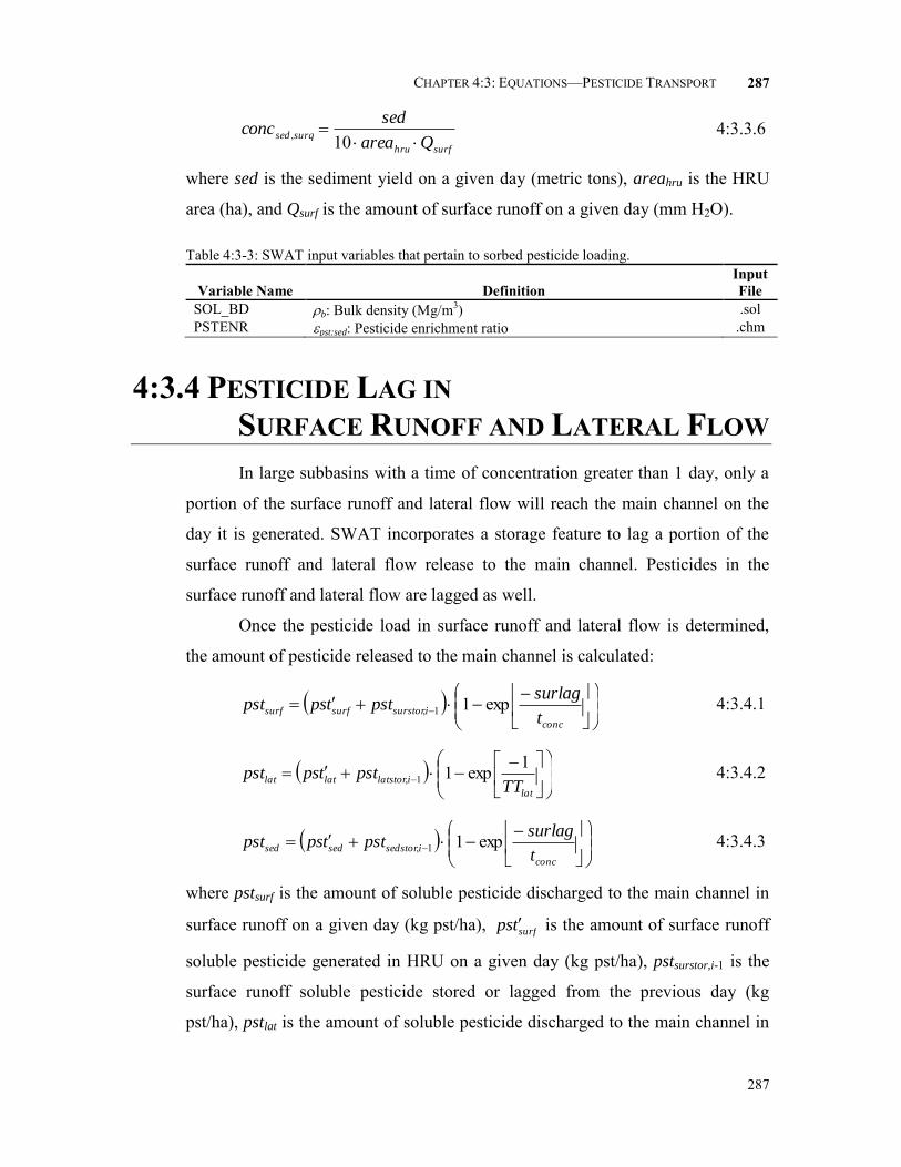
CHAPTER 4:3: EQUATIONS—PESTICIDE TRANSPORT
287
287
surfhru
surqsedQarea
sedconc
10, 4:3.3.6
where sed is the sediment yield on a given day (metric tons), areahru is the HRU
area (ha), and Qsurf is the amount of surface runoff on a given day (mm H2O).
Table 4:3-3: SWAT input variables that pertain to sorbed pesticide loading.
Variable Name
Definition Input File
SOL_BD b: Bulk density (Mg/m3) .sol PSTENR pst:sed: Pesticide enrichment ratio .chm
4:3.4 PESTICIDE LAG IN SURFACE RUNOFF AND LATERAL FLOW
In large subbasins with a time of concentration greater than 1 day, only a
portion of the surface runoff and lateral flow will reach the main channel on the
day it is generated. SWAT incorporates a storage feature to lag a portion of the
surface runoff and lateral flow release to the main channel. Pesticides in the
surface runoff and lateral flow are lagged as well.
Once the pesticide load in surface runoff and lateral flow is determined,
the amount of pesticide released to the main channel is calculated:
conc
isurstorsurfsurft
surlagpsttpspst exp11, 4:3.4.1
lat
ilatstorlatlatTT
psttpspst1exp11, 4:3.4.2
conc
isedstorsedsedt
surlagpsttpspst exp11, 4:3.4.3
where pstsurf is the amount of soluble pesticide discharged to the main channel in
surface runoff on a given day (kg pst/ha), surftps is the amount of surface runoff
soluble pesticide generated in HRU on a given day (kg pst/ha), pstsurstor,i-1 is the
surface runoff soluble pesticide stored or lagged from the previous day (kg
pst/ha), pstlat is the amount of soluble pesticide discharged to the main channel in

288 SWAT THEORETICAL DOCUMENTATION, VERSION 2009
288
lateral flow on a given day (kg pst/ha), lattps is the amount of lateral flow soluble
pesticide generated in HRU on a given day (kg pst/ha), pstlatstor,i-1 is the lateral
flow pesticide stored or lagged from the previous day (kg pst/ha), pstsed is the
amount of sorbed pesticide discharged to the main channel in surface runoff on a
given day (kg pst/ha), sedtps is the sorbed pesticide loading generated in HRU on
a given day (kg pst/ha), pstsedstor,i-1 is the sorbed pesticide stored or lagged from
the previous day (kg pst/ha), surlag is the surface runoff lag coefficient, tconc is the
time of concentration for the HRU (hrs) and TTlag is the lateral flow travel time
(days).
Table 4:3-4: SWAT input variables that pertain to pesticide lag calculations.
Variable Name
Definition Input File
SURLAG surlag: surface runoff lag coefficient .bsn LAT_TTIME TTlag: Lateral flow travel time (days) .hru
4:3.5 NOMENCLATURE
Csolidphase Concentration of the pesticide sorbed to the solid phase (mg/kg or g/ton) Csolution Concentration of the pesticide in solution (mg/L or g/ton) Koc Soil adsorption coefficient normalized for soil organic carbon content (ml/g or
(mg/kg)/(mg/L) or L/kg) Kp Soil adsorption coefficient ((mg/kg)/(mg/L)) Qlat Lateral flow from soil layer (mm H2O) Qsurf Accumulated runoff or rainfall excess (mm H2O) SATly Soil water content of layer ly at saturation (mm H2O) TTlag Lateral flow travel time (days) areahru HRU area (ha) concpst,flow Concentration of pesticide in the mobile water (kg pst/ha-mm H2O) concsed,surq Concentration of sediment in surface runoff (Mg sed/m3 H2O) depthly Depth of the soil layer (mm) orgCly Amount of organic carbon in the layer (%) pstflow Amount of pesticide removed in the flow (kg pst/ha) pstlat,ly Pesticide removed in lateral flow from a layer (kg pst/ha)
lattps Amount of lateral flow soluble pesticide generated in HRU on a given day (kg pst/ha)
pstlatstor,i-1 Lateral flow pesticide stored or lagged from the previous day (kg pst/ha) pstperc,ly Pesticide moved to the underlying layer by percolation (kg pst/ha) psts,ly Amount of pesticide in the soil (kg pst/ha)

CHAPTER 4:3: EQUATIONS—PESTICIDE TRANSPORT
289
289
pstsed Amount of sorbed pesticide transported to the main channel in surface runoff (kg pst/ha)
sedtps Sorbed pesticide loading generated in HRU on a given day (kg pst/ha) pstsedstor,i-1 Sorbed pesticide stored or lagged from the previous day (kg pst/ha) pstsol Solubility of the pesticide in water (mg/L) pstsurf Pesticide removed in surface runoff (kg pst/ha)
surftps Amount of surface runoff soluble pesticide generated in HRU on a given day (kg pst/ha)
pstsurstor,i-1 Surface runoff soluble pesticide stored or lagged from the previous day (kg pst/ha)
sed Sediment yield on a given day (metric tons) surlag Surface runoff lag coefficient tconc Time of concentration for a subbasin (hr) wmobile Amount of mobile water in the layer (mm H2O) wperc,ly Amount of water percolating to the underlying soil layer on a given day (mm
H2O) pst Pesticide percolation coefficient pst:sed Pesticide enrichment ratio b Soil bulk density (Mg m-3) w Density of water (1 Mg m-3)
4:3.6 REFERENCES
McElroy, A.D., S.Y. Chiu, J.W. Nebgen, A. Aleti, and F.W. Bennett. 1976.
Loading functions for assessment of water pollution from nonpoint
sources. Environ. Prot. Tech. Serv., EPA 600/2-76-151.
Menzel, R.G. 1980. Enrichment ratios for water quality modeling. p. 486-492. In
W.G. Knisel (ed.) CREAMS, A field scale model for chemicals, runoff,
and erosion from agricultural management systems. U.S. Dept. Agric.
Conserv. Res. Rept. No. 26.
Williams, J.R. 1995. Chapter 25: The EPIC model. p. 909-1000. In V.P. Singh
(ed.). Computer models of watershed hydrology. Water Resources
Publications.
Williams, J.R. and R.W. Hann. 1978. Optimal operation of large agricultural
watersheds with water quality constraints. Texas Water Resources
Institute, Texas A&M Univ., Tech. Rept. No. 96.

290 SWAT THEORETICAL DOCUMENTATION, VERSION 2009
290
291
SECTION 4 CHAPTER 4
EQUATIONS:
BACTERIA TRANSPORT
The transport of pathogenic bacteria from land areas into streams and
water bodies is a matter of concern in some watersheds. Excessive loading of
bacteria into streams and water bodies could potentially contaminate drinking
water and cause outbreaks of infection among the human population using the
water. This chapter reviews the algorithms governing movement of bacteria from
land areas to the stream network.

292 SWAT THEORETICAL DOCUMENTATION, VERSION 2009
292
4:4.1 BACTERIA IN SURFACE RUNOFF Due to the low mobility of bacteria in soil solution, surface runoff will
only partially interact with the bacteria present in the soil solution. The amount of
bacteria transported in surface runoff is:
surfbactsurfb
surflpsol
surflpkdepth
Qbactbact
,,
4:4.1.1
surfbactsurfb
surfpsol
surfpkdepth
Qbactbact
,,
4:4.1.2
where bactlp,surf is the amount of less persistent bacteria lost in surface runoff
(#cfu/m2), bactp,surf is the amount of persistent bacteria lost in surface runoff
(#cfu/m2), bactlpsol is the amount of less persistent bacteria present in soil solution
(#cfu/m2), bactpsol is the amount of persistent bacteria present in soil solution
(#cfu/m2), Q,surf is the amount of surface runoff on a given day (mm H2O), b is
the bulk density of the top 10 mm (Mg/m3) (assumed to be equivalent to bulk
density of first soil layer), depthsurf is the depth of the “surface” layer (10 mm),
and kbact,surf is the bacteria soil partitioning coefficient (m3/Mg). The bacteria soil
partitioning coefficient is the ratio of the bacteria concentration in the surface 10
mm soil solution to the concentration of bacteria in surface runoff.
Table 4:4-1: SWAT input variables that pertain to bacteria in surface runoff.
Variable Name
Definition Input File
SOL_BD b: Bulk density (Mg/m3) .sol BACTKDQ kbact,surf: Bacteria soil partitioning coefficient (m3/Mg) .bsn
4:4.2 BACTERIA ATTACHED TO SEDIMENT IN SURFACE RUNOFF
Bacteria attached to soil particles may be transported by surface runoff to
the main channel. This bacteria is associated with the sediment loading from the
HRU and changes in sediment loading will be reflected in the loading of this form
of bacteria. The amount of bacteria transported with sediment to the stream is
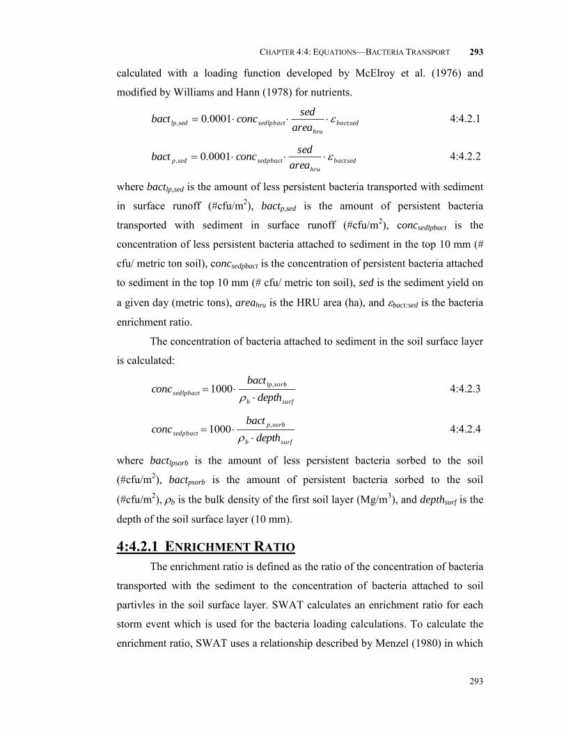
CHAPTER 4:4: EQUATIONS—BACTERIA TRANSPORT
293
293
calculated with a loading function developed by McElroy et al. (1976) and
modified by Williams and Hann (1978) for nutrients.
sedbact
hru
sedlpbactsedlparea
sedconcbact :, 0001.0 4:4.2.1
sedbact
hru
sedpbactsedparea
sedconcbact :, 0001.0 4:4.2.2
where bactlp,sed is the amount of less persistent bacteria transported with sediment
in surface runoff (#cfu/m2), bactp,sed is the amount of persistent bacteria
transported with sediment in surface runoff (#cfu/m2), concsedlpbact is the
concentration of less persistent bacteria attached to sediment in the top 10 mm (#
cfu/ metric ton soil), concsedpbact is the concentration of persistent bacteria attached
to sediment in the top 10 mm (# cfu/ metric ton soil), sed is the sediment yield on
a given day (metric tons), areahru is the HRU area (ha), and bact:sed is the bacteria
enrichment ratio.
The concentration of bacteria attached to sediment in the soil surface layer
is calculated:
surfb
sorblp
sedlpbactdepth
bactconc
,1000 4:4.2.3
surfb
sorbp
sedpbactdepth
bactconc
,1000 4:4.2.4
where bactlpsorb is the amount of less persistent bacteria sorbed to the soil
(#cfu/m2), bactpsorb is the amount of persistent bacteria sorbed to the soil
(#cfu/m2), b is the bulk density of the first soil layer (Mg/m3), and depthsurf is the
depth of the soil surface layer (10 mm).
4:4.2.1 ENRICHMENT RATIO The enrichment ratio is defined as the ratio of the concentration of bacteria
transported with the sediment to the concentration of bacteria attached to soil
partivles in the soil surface layer. SWAT calculates an enrichment ratio for each
storm event which is used for the bacteria loading calculations. To calculate the
enrichment ratio, SWAT uses a relationship described by Menzel (1980) in which
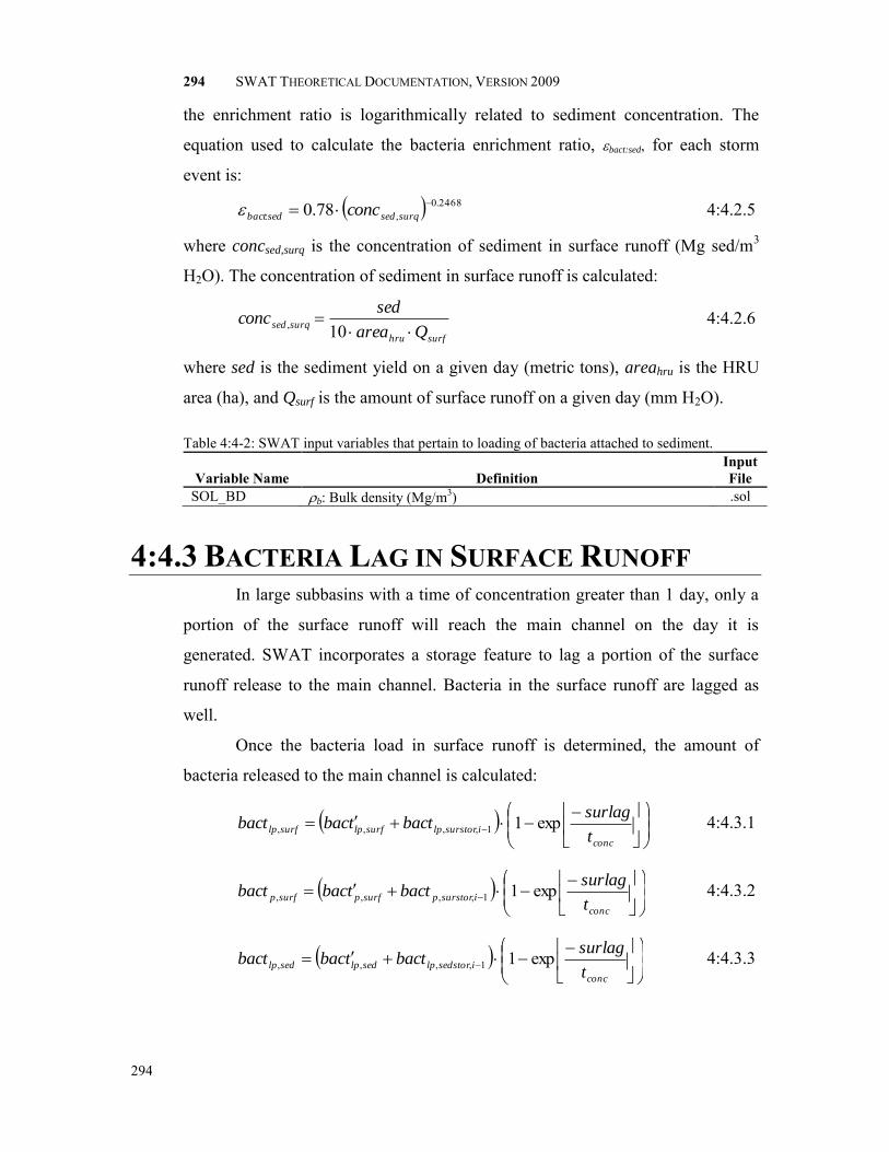
294 SWAT THEORETICAL DOCUMENTATION, VERSION 2009
294
the enrichment ratio is logarithmically related to sediment concentration. The
equation used to calculate the bacteria enrichment ratio, bact:sed, for each storm
event is:
2468.0,: 78.0
surqsedsedbact conc 4:4.2.5
where concsed,surq is the concentration of sediment in surface runoff (Mg sed/m3
H2O). The concentration of sediment in surface runoff is calculated:
surfhru
surqsedQarea
sedconc
10, 4:4.2.6
where sed is the sediment yield on a given day (metric tons), areahru is the HRU
area (ha), and Qsurf is the amount of surface runoff on a given day (mm H2O).
Table 4:4-2: SWAT input variables that pertain to loading of bacteria attached to sediment.
Variable Name
Definition Input File
SOL_BD b: Bulk density (Mg/m3) .sol
4:4.3 BACTERIA LAG IN SURFACE RUNOFF In large subbasins with a time of concentration greater than 1 day, only a
portion of the surface runoff will reach the main channel on the day it is
generated. SWAT incorporates a storage feature to lag a portion of the surface
runoff release to the main channel. Bacteria in the surface runoff are lagged as
well.
Once the bacteria load in surface runoff is determined, the amount of
bacteria released to the main channel is calculated:
conc
isurstorlpsurflpsurflpt
surlagbacttbacbact exp11,,,, 4:4.3.1
conc
isurstorpsurfpsurfpt
surlagbacttbacbact exp11,,,, 4:4.3.2
conc
isedstorlpsedlpsedlpt
surlagbacttbacbact exp11,,,, 4:4.3.3

CHAPTER 4:4: EQUATIONS—BACTERIA TRANSPORT
295
295
conc
isedstorpsedpsedpt
surlagbacttbacbact exp11,,,, 4:4.3.4
where bactlp,surf is the amount of less persistent bacteria discharged to the main
channel in surface runoff on a given day (#cfu/m2), surflptbac , is the amount of
surface runoff less persistent bacteria generated in the HRU on a given day
(#cfu/m2), bactlp,surstor,i-1 is the surface runoff less persistent bacteria stored or
lagged from the previous day (#cfu/m2), bactp,surf is the amount of persistent
bacteria discharged to the main channel in surface runoff on a given day
(#cfu/m2), surfptbac , is the amount of surface runoff persistent bacteria generated
in the HRU on a given day (#cfu/m2), bactp,surstor,i-1 is the surface runoff persistent
bacteria stored or lagged from the previous day (#cfu/m2), bactlp,sed is the amount
of sediment-attached less persistent bacteria discharged to the main channel in
surface runoff on a given day (#cfu/m2), sedlptbac , is the amount of sediment-
attached less persistent bacteria generated in the HRU on a given day (#cfu/m2),
bactlp,sedstor,i-1 is the sediment-attached less persistent bacteria stored or lagged
from the previous day (#cfu/m2), bactp,sed is the amount of sediment-attached
persistent bacteria discharged to the main channel in surface runoff on a given day
(#cfu/m2), sedptbac , is the amount of sediment-attached persistent bacteria
generated in the HRU on a given day (#cfu/m2), bactp,sedstor,i-1 is the sediment-
attached persistent bacteria stored or lagged from the previous day (#cfu/m2),
surlag is the surface runoff lag coefficient, and tconc is the time of concentration
for the HRU (hrs).
Table 4:4-3: SWAT input variables that pertain to bacteria lag calculations.
Variable Name
Definition Input File
SURLAG surlag: surface runoff lag coefficient .bsn

296 SWAT THEORETICAL DOCUMENTATION, VERSION 2009
296
4:4.4 NOMENCLATURE Qsurf Accumulated runoff or rainfall excess (mm H2O)
areahru HRU area (ha) sedlptbac , Amount of sediment-attached less persistent bacteria generated in the HRU on a
given day (#cfu/m2) bactlp,sed Amount of less persistent bacteria transported with sediment in surface runoff
(#cfu/m2) bactlp,sedstor,i-1 Sediment-attached less persistent bacteria stored or lagged from the
previous day (#cfu/m2) bactlpsol Amount of less persistent bacteria present in soil solution (#cfu/m2) bactlpsorb Amount of less persistent bacteria sorbed to the soil (#cfu/m2)
surflptbac , Amount of surface runoff less persistent bacteria generated in the HRU on a given day (#cfu/m2)
bactlp,surf Amount of less persistent bacteria lost in surface runoff (#cfu/m2) bactlp,surstor,i-1 Surface runoff less persistent bacteria stored or lagged from the previous
day (#cfu/m2) sedptbac , Amount of sediment-attached persistent bacteria generated in the HRU on a
given day (#cfu/m2) bactp,sed Amount of persistent bacteria transported with sediment in surface runoff
(#cfu/m2) bactp,sedstor,i-1 Sediment-attached persistent bacteria stored or lagged from the previous day
(#cfu/m2) bactpsol Amount of persistent bacteria present in soil solution (#cfu/m2) bactpsorb Amount of persistent bacteria sorbed to the soil (#cfu/m2)
surfptbac , Amount of surface runoff persistent bacteria generated in the HRU on a given day (#cfu/m2)
bactp,surf Amount of persistent bacteria lost in surface runoff (#cfu/m2) bactp,surstor,i-1 Surface runoff persistent bacteria stored or lagged from the previous day
(#cfu/m2) concsedlpbact Concentration of less persistent bacteria attached to sediment in the top 10
mm (# cfu/ metric ton soil) concsedpbact Concentration of persistent bacteria attached to sediment in the top 10 mm (#
cfu/ metric ton soil) concsed,surq Concentration of sediment in surface runoff (Mg sed/m3 H2O) depthsurf Depth of the “surface” layer (10 mm) kbact,surf Bacteria soil partitioning coefficient (m3/Mg) sed Sediment yield on a given day (metric tons) surlag Surface runoff lag coefficient tconc Time of concentration for a subbasin (hr)
bact:sed Bacteria enrichment ratio
b Bulk density (Mg/m3)

CHAPTER 4:4: EQUATIONS—BACTERIA TRANSPORT
297
297

298
SECTION 4 CHAPTER 5
EQUATIONS:
WATER QUALITY PARAMETERS
In addition to sediment, nutrients and pesticides, SWAT will calculate the
amount of algae, dissolved oxygen and carbonaceous biological oxygen demand
(CBOD) entering the main channel with surface runoff. Loadings of these three
parameters impact the quality of stream water. This chapter reviews the
algorithms governing movement of algae, dissolved oxygen and CBOD from land
areas to the stream network. Because the algorithms were based on very limited
field data, calculation of these loadings has been made optional.

CHAPTER 4:5: EQUATIONS—WATER QUALITY PARAMETERS
299
299
4:5.1 ALGAE Suspended algal biomass is assumed to be directly proportional to
chlorophyll a. Therefore, the algal biomass loading to the stream can be estimated
as the chlorophyll a loading from the land area. Cluis et al. (1988) developed a
relationship between the nutrient enrichment index (total N: total P), chlorophyll
a, and algal growth potential in the North Yamaska River, Canada.
g
surfTP
TNfvchlaAGP
4:5.1.1
where AGP is the algal growth potential (mg/L), chla is the chlorophyll a
concentration in the surface runoff (μg/L), vsurf is the surface runoff flow rate
(m3/s), TN is the total Kjeldahl nitrogen load (kmoles), TP is the total phosphorus
load (kmoles), f is a coefficient and g is an exponent.
The chlorophyll a concentration in surface runoff is calculated in SWAT
using a simplified version of Cluis et al.’s exponential function (1988):
0chla if ( /sm 10 35surfv ) or ( 610 and TNTP ) 4:5.1.2
surfvchla
7.2105.0 if /sm 10 35surfv , and ( 610 and TNTP ) 4:5.1.3
surfvchla
5.0105.0 if /sm 10 35surfv , 610TP and 610TN 4:5.1.4
4:5.2 CARBONACEOUS BIOLOGICAL OXYGEN DEMAND
Carbonaceous biological oxygen demand (CBOD) defines the amount of
oxygen required to decompose the organic matter transported in surface runoff.
The SWAT loading function for CBOD is based on a relationship given by
Thomann and Mueller (1987):
hrusurf
surq
surqareaQ
orgCcbod
7.2 4:5.2.1

300 SWAT THEORETICAL DOCUMENTATION, VERSION 2009
300
where cbodsurq is the CBOD concentration in surface runoff (mg CBOD/L),
orgCsurq is the organic carbon in surface runoff (kg orgC), Qsurf is the surface
runoff on a given day (mm H2O), and areahru is the area of the HRU (km2).
The amount of organic carbon in surface runoff is calculated:
sedC
surf
surq sedorgC
orgC :1001000 4:5.2.2
where orgCsurq is the organic carbon in surface runoff (kg orgC), orgCsurf is the
percent organic carbon in the top 10 mm of soil (%), sed is the sediment loading
from the HRU (metric tons), and C:sed is the carbon enrichment ratio.
4:5.2.1 ENRICHMENT RATIO As runoff flows over the soil surface, part of the water’s energy is used to
pick up and transport soil particles. The smaller particles weigh less and are more
easily transported than coarser particles. When the particle size distribution of the
transported sediment is compared to that of the soil surface layer, the sediment
load to the main channel has a greater proportion of clay sized particles. In other
words, the sediment load is enriched in clay particles. Organic carbon in the soil is
attached primarily to colloidal (clay) particles, so the sediment load will also
contain a greater proportion or concentration of organic carbon than that found in
the soil surface layer.
The enrichment ratio is defined as the ratio of the concentration of organic
carbon transported with the sediment to the concentration in the soil surface layer.
SWAT will calculate an enrichment ratio for each storm event. To calculate the
enrichment ratio, SWAT uses a relationship described by Menzel (1980) in which
the enrichment ratio is logarithmically related to sediment concentration. The
equation used to calculate the carbon enrichment ratio, C:sed, for each storm event
is:
2468.0,: 78.0
surqsedsedC conc 4:5.2.3
where concsed,surq is the concentration of sediment in surface runoff (Mg sed/m3
H2O). The concentration of sediment in surface runoff is calculated:

CHAPTER 4:5: EQUATIONS—WATER QUALITY PARAMETERS
301
301
surfhru
surqsedQarea
sedconc
10, 4:5.2.4
where sed is the sediment yield on a given day (metric tons), areahru is the HRU
area (ha), and Qsurf is the amount of surface runoff on a given day (mm H2O).
Table 4:5-1: SWAT input variables that pertain to CBOD in surface runoff.
Variable Name
Definition Input File
SOL_CBN orgCly: Percent organic carbon in the top 10 mm of soil (%) .sol
4:5.3 DISSOLVED OXYGEN Rainfall is assumed to be saturated with oxygen. To determine the
dissolved oxygen concentration of surface runoff, the oxygen uptake by the
oxygen demanding substance in runoff is subtracted from the saturation oxygen
concentration.
241ov
surqsatsurf
tcbodOxOx 4:5.3.1
where Oxsurf is the dissolved oxygen concentration in surface runoff (mg O2/L),
Oxsat is the saturation oxygen concentration (mg O2/L), 1 is the CBOD
deoxygenation rate (day-1), cbodsurq is the CBOD concentration in surface runoff
(mg CBOD/L), and tov is the time of concentration for overland flow (hr). For
loadings from HRUs, SWAT assumes 1 = 1.047 day-1.
4:5.3.1 OXYGEN SATURATION CONCENTRATION
The amount of oxygen that can be dissolved in water is a function of
temperature, concentration of dissolved solids, and atmospheric pressure. An
equation developed by APHA (1985) is used to calculate the saturation
concentration of dissolved oxygen:
2,
7
,
5 10642308.610575701.134410.139expKwatKwat
satTT
Ox
4
,
11
3,
10 10621949.810243800.1
KwatKwat TT 4:5.3.2

302 SWAT THEORETICAL DOCUMENTATION, VERSION 2009
302
where Oxsat is the equilibrium saturation oxygen concentration at 1.00 atm (mg O2/L), and Twat,K is the water temperature in Kelvin (273.15+C).
4:5.4 NOMENCLATURE
AGP Algal growth potential (mg/L) Oxsat Saturation oxygen concentration (mg O2/L) Oxsurf Dissolved oxygen concentration in surface runoff (mg O2/L) Qsurf Surface runoff on a given day (mm H2O) Twat,K Water temperature in Kelvin (273.15+C) TN Total Kjeldahl nitrogen load (moles) TP Total phosphorus load (moles)
areahru Area of the HRU (km2) cbodsurq CBOD concentration in surface runoff (mg CBOD/L) chla Chlorophyll a concentration in the surface runoff (μg/L) concsed,surq Concentration of sediment in surface runoff (Mg sed/m3 H2O) f Coefficient g Exponent orgCsurf Percent organic carbon in the top 10 mm of soil (%) orgCsurq Organic carbon in surface runoff (kg orgC), sed Sediment loading from the HRU (metric tons) tov Time of concentration for overland flow (hr) vsurf Surface runoff flow rate (m3/s)
C:sed Carbon enrichment ratio
1 CBOD deoxygenation rate (day-1)
4:5.5 REFERENCES
American Public Health Association. 1985. Standard methods for the examination of water and wastewater, 16th edition. American Public Health Association, Inc.
Cluis, D., P. Couture, R. Bégin, and S.A. Visser. 1988. Potential eutrophication assessment in rivers; relationship between produced and exported loads. Schweiz. Z. Hydrol. 50:166-181.
Menzel, R.G. 1980. Enrichment ratios for water quality modeling. p. 486-492. In W.G. Knisel (ed.) CREAMS, A field scale model for chemicals, runoff, and erosion from agricultural management systems. U.S. Dept. Agric. Conserv. Res. Rept. No. 26.
Thomann, R.V. and J.A. Mueller. 1987. Principles of surface water quality modeling and control. Harper & Row Publishers, New York.

CHAPTER 4:5: EQUATIONS—WATER QUALITY PARAMETERS
303
303

LAND COVER & PLANT
The plant growth component of SWAT is a
simplified version of the EPIC plant growth model. As
in EPIC, phenological plant development is based on
daily accumulated heat units, potential biomass is based
on a method developed by Monteith, a harvest index is
used to calculate yield, and plant growth can be
inhibited by temperature, water, nitrogen or phosphorus
stress. Portions of the EPIC plant growth model that
were not incorporated into SWAT include detailed root
growth, micronutrient cycling and toxicity responses,
and the simultaneous growth of multiple plant species in
the same HRU.

304
SECTION 5 CHAPTER 1
EQUATIONS:
GROWTH CYCLE
The growth cycle of a plant is controlled by plant attributes summarized in
the plant growth database and by the timing of operations listed in the
management file. This chapter reviews the heat unit theory used to regulate the
growth cycle of plants. Chapter 6:1 focuses on the impact of user inputs in
management operations on the growth and development of plants.

CHAPTER 5:1: EQUATIONS—GROWTH CYCLE
305
305
5:1.1 HEAT UNITS
Temperature is one of the most important factors governing plant growth.
Each plant has its own temperature range, i.e. its minimum, optimum, and
maximum for growth. For any plant, a minimum or base temperature must be
reached before any growth will take place. Above the base temperature, the higher
the temperature the more rapid the growth rate of the plant. Once the optimum
temperature is exceeded the growth rate will begin to slow until a maximum
temperature is reached at which growth ceases.
In the 1920s and 1930s, canning factories were searching for ways to time
the planting of sweet peas so that there would be a steady flow of peas at the peak
of perfection to the factory. Crops planted at weekly intervals in the early spring
would sometimes come to maturity with only a 1- or 2-day differential while at
other times there was a 6- to 8-day differential (Boswell, 1926; 1929). A heat unit
theory was suggested (Boswell, 1926; Magoon and Culpepper, 1932) that was
revised and successfully applied (Barnard, 1948; Phillips, 1950) by canning
companies to determine when plantings should be made to ensure a steady harvest
of peas with no ―bunching‖ or ―breaks‖.
The heat unit theory postulates that plants have heat requirements that can
be quantified and linked to time to maturity. Because a plant will not grow when
the mean temperature falls below its base temperature, the only portion of the
mean daily temperature that contributes towards the plant’s development is the
amount that exceeds the base temperature. To measure the total heat requirements
of a plant, the accumulation of daily mean air temperatures above the plant’s base
temperature is recorded over the period of the plant’s growth and expressed in
terms of heat units. For example, assume sweet peas are growing with a base
temperature of 5C. If the mean temperature on a given day is 20C, the heat units
accumulated on that day are 20 – 5 = 15 heat units. Knowing the planting date,
maturity date, base temperature and mean daily temperatures, the total number of
heat units required to bring a crop to maturity can be calculated.

306 SWAT THEORETICAL DOCUMENTATION, VERSION 2009
306
The heat index used by SWAT is a direct summation index. Each degree
of the daily mean temperature above the base temperature is one heat unit. This
method assumes that the rate of growth is directly proportional to the increase in
temperature. It is important to keep in mind that the heat unit theory without a
high temperature cutoff does not account for the impact of harmful high
temperatures. SWAT assumes that all heat above the base temperature accelerates
crop growth and development.
Figure 5:1-1: Mean daily temperature recorded for Greenfield, Indiana The mean daily temperature during 1992 for Greenfield, Indiana is plotted
in Figure 5:1-1 along with the base temperature for corn (8C). Crop growth will
only occur on those days where the mean daily temperature exceeds the base
temperature. The heat unit accumulation for a given day is calculated with the
equation:
baseav TTHU when baseav TT 5:1.1.1
where HU is the number of heat units accumulated on a given day (heat units),
avT is the mean daily temperature (C), and Tbase is the plant’s base or minimum
-20
-10
0
10
20
30
1/1/
1992
1/15
/199
2
1/29
/199
2
2/12
/199
2
2/26
/199
2
3/11
/199
2
3/25
/199
2
4/8/
1992
4/22
/199
2
5/6/
1992
5/20
/199
2
6/3/
1992
6/17
/199
2
7/1/
1992
7/15
/199
2
7/29
/199
2
8/12
/199
2
8/26
/199
2
9/9/
1992
9/23
/199
2
10/7
/199
2
10/2
1/19
92
11/4
/199
2
11/1
8/19
92
12/2
/199
2
12/1
6/19
92
12/3
0/19
92
Tem
pera
ture
(d
eg
C)
Date
Mean daily temperature Base temperature, corn
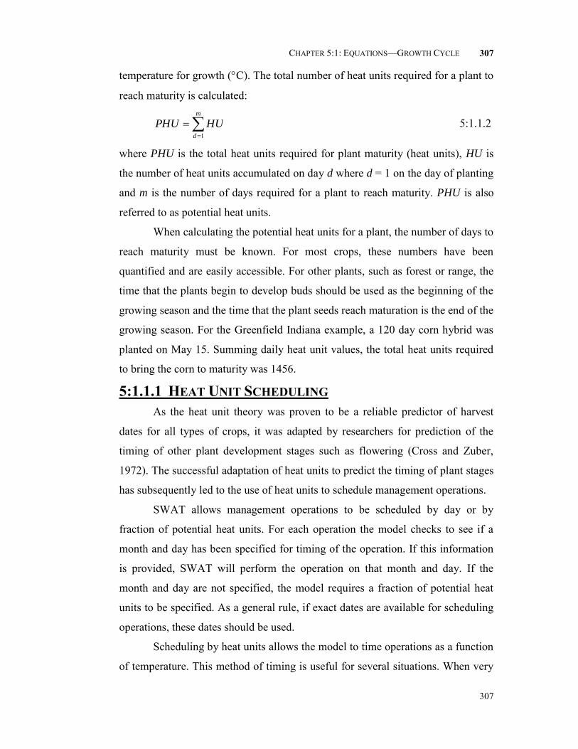
CHAPTER 5:1: EQUATIONS—GROWTH CYCLE
307
307
temperature for growth (C). The total number of heat units required for a plant to
reach maturity is calculated:
m
d
HUPHU1
5:1.1.2
where PHU is the total heat units required for plant maturity (heat units), HU is
the number of heat units accumulated on day d where d = 1 on the day of planting
and m is the number of days required for a plant to reach maturity. PHU is also
referred to as potential heat units.
When calculating the potential heat units for a plant, the number of days to
reach maturity must be known. For most crops, these numbers have been
quantified and are easily accessible. For other plants, such as forest or range, the
time that the plants begin to develop buds should be used as the beginning of the
growing season and the time that the plant seeds reach maturation is the end of the
growing season. For the Greenfield Indiana example, a 120 day corn hybrid was
planted on May 15. Summing daily heat unit values, the total heat units required
to bring the corn to maturity was 1456.
5:1.1.1 HEAT UNIT SCHEDULING As the heat unit theory was proven to be a reliable predictor of harvest
dates for all types of crops, it was adapted by researchers for prediction of the
timing of other plant development stages such as flowering (Cross and Zuber,
1972). The successful adaptation of heat units to predict the timing of plant stages
has subsequently led to the use of heat units to schedule management operations.
SWAT allows management operations to be scheduled by day or by
fraction of potential heat units. For each operation the model checks to see if a
month and day has been specified for timing of the operation. If this information
is provided, SWAT will perform the operation on that month and day. If the
month and day are not specified, the model requires a fraction of potential heat
units to be specified. As a general rule, if exact dates are available for scheduling
operations, these dates should be used.
Scheduling by heat units allows the model to time operations as a function
of temperature. This method of timing is useful for several situations. When very

308 SWAT THEORETICAL DOCUMENTATION, VERSION 2009
308
large watersheds are being simulated where the climate in one portion of the
watershed is different enough from the climate in another section of the watershed
to affect timing of operations, heat unit scheduling may be beneficial. By using
heat unit scheduling, only one generic management file has to be made for a given
land use. This generic set of operations can then be used wherever the land use is
found in the watershed. Also, in areas where the climate can vary greatly from
year to year, heat unit scheduling will allow the model to adjust the timing of
operations to the weather conditions for each year.
While scheduling by heat units is convenient, there are some negatives to
using this type of scheduling that users need to take into consideration. In the real
world, applications of fertilizer or pesticide are generally not scheduled on a rainy
day. However when applications are scheduled by heat units, the user has no
knowledge of whether or not the heat unit fraction that triggers the application
will occur on a day with rainfall or not. If they do coincide, there will be a
significant amount of the applied material transported with surface runoff
(assuming runoff is generated on that day), much higher than if the application
took place even one day prior to the rainfall event.
To schedule by heat units, the timing of the operations are expressed as
fractions of the potential heat units for the plant or fraction of maturity. Let us use
the following example for corn in Indiana.
Date Operation Heat Units Accumulated
Fraction of PHU
April 24 Tandem disk April 30 Tandem disk May 7 Field cultivator May 15 Plant corn (PHU = 1456) 0 .00 June 3 Row cultivator 165 .11 June 17 Row cultivator 343 .24 October 15 Harvest & Kill 1686 1.16 October 29 Tandem disk November 5 Chisel
The number of heat units accumulated for the different operation timings
is calculated by summing the heat units for every day starting with the planting
date (May 15) and ending with the day the operation takes place. To calculate the

CHAPTER 5:1: EQUATIONS—GROWTH CYCLE
309
309
fraction of PHU at which the operation takes place, the heat units accumulated is
divided by the PHU for the crop (1456).
Note that the fraction of PHU for the harvest operation is 1.16. The
fraction is greater than 1.0 because corn is allowed to dry down prior to
harvesting. The model will simulate plant growth until the crop reaches maturity
(where maturity is defined as PHU = 1456). From that point on, plants will not
transpire or take up nutrients and water. They will stand in the HRU until
converted to residue or harvested.
While the operations after planting have been scheduled by fraction of
PHU, operations—including planting—which occur during periods when no crop
is growing must still be scheduled. To schedule these operations, SWAT keeps
track of a second heat index where heat units are summed over the entire year
using Tbase = 0C. This heat index is solely a function of the climate and is termed
the base zero heat index. For the base zero index, the heat units accumulated on a
given day are:
avTHU 0 when avT 0C 5:1.1.3
where HU0 is the number of base zero heat units accumulated on a given day
(heat units), and avT is the mean daily temperature (C). The total number of heat
units for the year is calculated:
365
100
d
HUPHU 5:1.1.4
where PHU0 is the total base zero heat units (heat units), HU0 is the number of
base zero heat units accumulated on day d where d = 1 on January 1 and 365 on
December 31. Unlike the plant PHU which must be provided by the user, PHU0 is
the average calculated by SWAT using long-term weather data provided in the
.wgn file.
For the example watershed in Indiana, PHU0 = 4050. The heat unit
fractions for the remaining operations are calculated using this value for potential
heat units.
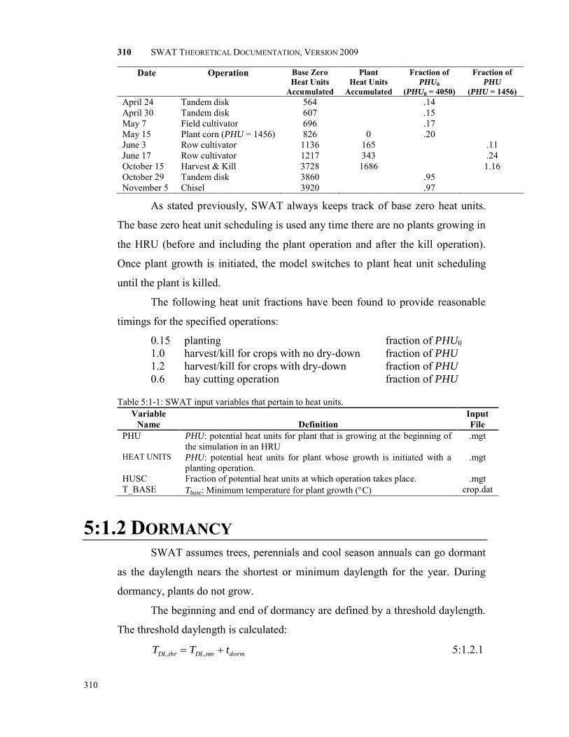
310 SWAT THEORETICAL DOCUMENTATION, VERSION 2009
310
Date Operation Base Zero Heat Units
Accumulated
Plant Heat Units
Accumulated
Fraction of PHU0
(PHU0 = 4050)
Fraction of PHU
(PHU = 1456) April 24 Tandem disk 564 .14 April 30 Tandem disk 607 .15 May 7 Field cultivator 696 .17 May 15 Plant corn (PHU = 1456) 826 0 .20 June 3 Row cultivator 1136 165 .11 June 17 Row cultivator 1217 343 .24 October 15 Harvest & Kill 3728 1686 1.16 October 29 Tandem disk 3860 .95 November 5 Chisel 3920 .97
As stated previously, SWAT always keeps track of base zero heat units.
The base zero heat unit scheduling is used any time there are no plants growing in
the HRU (before and including the plant operation and after the kill operation).
Once plant growth is initiated, the model switches to plant heat unit scheduling
until the plant is killed.
The following heat unit fractions have been found to provide reasonable
timings for the specified operations:
0.15 planting fraction of PHU0 1.0 harvest/kill for crops with no dry-down fraction of PHU 1.2 harvest/kill for crops with dry-down fraction of PHU 0.6 hay cutting operation fraction of PHU
Table 5:1-1: SWAT input variables that pertain to heat units. Variable
Name
Definition Input File
PHU PHU: potential heat units for plant that is growing at the beginning of the simulation in an HRU
.mgt
HEAT UNITS PHU: potential heat units for plant whose growth is initiated with a planting operation.
.mgt
HUSC Fraction of potential heat units at which operation takes place. .mgt T_BASE Tbase: Minimum temperature for plant growth (C) crop.dat
5:1.2 DORMANCY SWAT assumes trees, perennials and cool season annuals can go dormant
as the daylength nears the shortest or minimum daylength for the year. During
dormancy, plants do not grow.
The beginning and end of dormancy are defined by a threshold daylength.
The threshold daylength is calculated:
dormmnDLthrDL tTT ,, 5:1.2.1

CHAPTER 5:1: EQUATIONS—GROWTH CYCLE
311
311
where TDL,thr is the threshold daylength to initiate dormancy (hrs), TDL,mn is the
minimum daylength for the watershed during the year (hrs), and tdorm is the
dormancy threshold (hrs). When the daylength becomes shorter than TDL,thr in the
fall, plants other than warm season annuals that are growing in the watershed will
enter dormancy. The plants come out of dormancy once the daylength exceeds
TDL,thr in the spring.
The dormancy threshold, tdorm, varies with latitude.
0.1dormt if > 40 º N or S 5:1.2.2
2020
dormt if 20 º N or S 40 º N or S 5:1.2.3
0.0dormt if < 20 º N or S 5:1.2.4
where tdorm is the dormancy threshold used to compare actual daylength to
minimum daylength (hrs) and is the latitude expressed as a positive value
(degrees).
At the beginning of the dormant period for trees, a fraction of the biomass
is converted to residue and the leaf area index for the tree species is set to the
minimum value allowed (both the fraction of the biomass converted to residue
and the minimum LAI are defined in the plant growth database). At the beginning
of the dormant period for perennials, 10% of the biomass is converted to residue
and the leaf area index for the species is set to the minimum value allowed. For
cool season annuals, none of the biomass is converted to residue.
Table 5:1-2: SWAT input variables that pertain to dormancy. Variable
Name
Definition Input File
SUB_LAT : Latitude of the subbasin (degrees). .sub IDC Land cover/plant classification:
1 warm season annual legume 2 cold season annual legume 3 perennial legume 4 warm season annual 5 cold season annual 6 perennial 7 trees
crop.dat
ALAI_MIN Minimum leaf area index for plant during dormant period (m2/m2) crop.dat BIO_LEAF Fraction of tree biomass accumulated each year that is converted to
residue during dormancy crop.dat

312 SWAT THEORETICAL DOCUMENTATION, VERSION 2009
312
5:1.3 PLANT TYPES SWAT categorizes plants into seven different types: warm season annual
legume, cold season annual legume, perennial legume, warm season annual, cold
season annual, perennial and trees. The differences between the different plant
types, as modeled by SWAT, are as follows:
1 warm season annual legume: simulate nitrogen fixation root depth varies during growing season due to root growth
2 cold season annual legume: simulate nitrogen fixation root depth varies during growing season due to root growth fall-planted land covers will go dormant when daylength is less
than the threshold daylength 3 perennial legume:
simulate nitrogen fixation root depth always equal to the maximum allowed for the plant
species and soil plant goes dormant when daylength is less than the threshold
daylength 4 warm season annual:
root depth varies during growing season due to root growth 5 cold season annual:
root depth varies during growing season due to root growth fall-planted land covers will go dormant when daylength is less
than the threshold daylength 6 perennial:
root depth always equal to the maximum allowed for the plant species and soil
plant goes dormant when daylength is less than the threshold daylength
7 trees: root depth always equal to the maximum allowed for the plant
species and soil partitions new growth between leaves/needles and woody growth growth in a given year will vary depending on the age of the tree
relative to the number of years required for the tree to full development/maturity
plant goes dormant when daylength is less than the threshold daylength

CHAPTER 5:1: EQUATIONS—GROWTH CYCLE
313
313
Table 5:1-3: SWAT input variables that pertain to plant type. Variable
Name
Definition Input File
IDC Land cover/plant classification: 1 warm season annual legume 2 cold season annual legume 3 perennial legume 4 warm season annual 5 cold season annual 6 perennial 7 trees
crop.dat
5:1.4 NOMENCLATURE HU Number of heat units accumulated on a given day where base temperature is
dependant on the plant species (heat units) HU0 Number of base zero heat units accumulated on a given day (heat units) PHU Potential heat units or total heat units required for plant maturity where base
temperature is dependant on the plant species (heat units) PHU0 Total base zero heat units or potential base zero heat units (heat units) Tbase Plant’s base or minimum temperature for growth (C) TDL,mn Minimum daylength for the watershed during the year (hrs) TDL,thr Threshold daylength to initiate dormancy (hrs)
avT Mean air temperature for day (C) tdorm Dormancy threshold (hrs) Latitude expressed as a positive value (degrees)
314 SWAT THEORETICAL DOCUMENTATION, VERSION 2009
314
5:1.5 REFERENCES
Barnard, J.D. 1948. Heat units as a measure of canning crop maturity. The Canner
106:28.
Boswell, V.G. 1929. Factors influencing yield and quality of peas—Biophysical
and biochemical studies. Maryland Agr. Exp. Sta. Bul. 306.
Boswell, V.G. 1926. The influence of temperature upon the growth and yield of
garden peas. Proc. Amer. Soc. Hort. Sci. 23:162-168.
Cross, H.Z. and M.S. Zuber. 1972. Prediction of flowering dates in maize based
on different methods of estimating thermal units. Agronomy Journal
64:351-355.
Magoon, C.A. and C.W. Culpepper. 1932. Response of sweet corn to varying
temperatures from time of planting to canning maturity. U.S.D.A. tech.
Bull. 312.
Phillips, E.E. 1950. Heat summation theory as applied to canning crops. The
Canner 27:13-15.

CHAPTER 5:1: EQUATIONS—GROWTH CYCLE
315
315

316
SECTION 5 CHAPTER 2
EQUATIONS:
OPTIMAL GROWTH
For each day of simulation, potential plant growth, i.e. plant growth under
ideal growing conditions, is calculated. Ideal growing conditions consist of
adequate water and nutrient supply and a favorable climate. Differences in growth
between plant species are defined by the parameters contained in the plant growth
database.
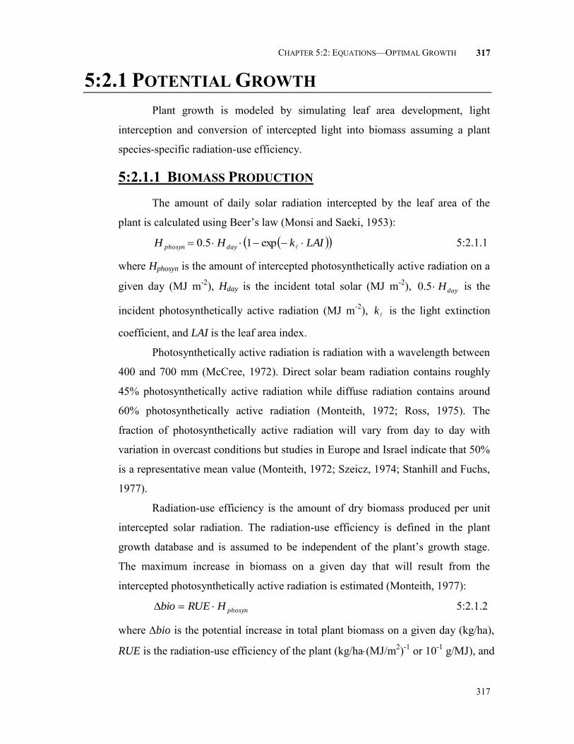
CHAPTER 5:2: EQUATIONS—OPTIMAL GROWTH
317
317
5:2.1 POTENTIAL GROWTH
Plant growth is modeled by simulating leaf area development, light
interception and conversion of intercepted light into biomass assuming a plant
species-specific radiation-use efficiency.
5:2.1.1 BIOMASS PRODUCTION The amount of daily solar radiation intercepted by the leaf area of the
plant is calculated using Beer’s law (Monsi and Saeki, 1953):
LAIkHH dayphosyn exp15.0 5:2.1.1
where Hphosyn is the amount of intercepted photosynthetically active radiation on a
given day (MJ m-2), Hday is the incident total solar (MJ m-2), dayH5.0 is the
incident photosynthetically active radiation (MJ m-2), k is the light extinction
coefficient, and LAI is the leaf area index.
Photosynthetically active radiation is radiation with a wavelength between
400 and 700 mm (McCree, 1972). Direct solar beam radiation contains roughly
45% photosynthetically active radiation while diffuse radiation contains around
60% photosynthetically active radiation (Monteith, 1972; Ross, 1975). The
fraction of photosynthetically active radiation will vary from day to day with
variation in overcast conditions but studies in Europe and Israel indicate that 50%
is a representative mean value (Monteith, 1972; Szeicz, 1974; Stanhill and Fuchs,
1977).
Radiation-use efficiency is the amount of dry biomass produced per unit
intercepted solar radiation. The radiation-use efficiency is defined in the plant
growth database and is assumed to be independent of the plant’s growth stage.
The maximum increase in biomass on a given day that will result from the
intercepted photosynthetically active radiation is estimated (Monteith, 1977):
phosynHRUEbio 5:2.1.2
where bio is the potential increase in total plant biomass on a given day (kg/ha),
RUE is the radiation-use efficiency of the plant (kg/ha(MJ/m2)-1 or 10-1 g/MJ), and

318 SWAT THEORETICAL DOCUMENTATION, VERSION 2009
318
Hphosyn is the amount of intercepted photosynthetically active radiation on a given
day (MJ m-2). Equation 5:2.1.2 assumes that the photosynthetic rate of a canopy is
a linear function of radiant energy.
The total biomass on a given day, d, is calculated as:
d
i
ibiobio1
5:2.1.3
where bio is the total plant biomass on a given day (kg ha-1), and bioi is the
increase in total plant biomass on day i (kg/ha).
5:2.1.1.1 IMPACT OF CLIMATE ON RADIATION-USE EFFICIENCY Radiation-use efficiency is sensitive to variations in atmospheric
CO2 concentrations and equations have been incorporated into SWAT to
modify the default radiation-use efficiency values in the plant database for
climate change studies. The relationship used to adjust the radiation-use
efficiency for effects of elevated CO2 is (Stockle et al., 1992):
2212
2
exp100
COrrCO
CORUE
5:2.1.4
where RUE is the radiation-use efficiency of the plant (kg/ha(MJ/m2)-1 or
10-1 g/MJ), CO2 is the concentration of carbon dioxide in the atmosphere
(ppmv), and r1 and r2 are shape coefficients.
The shape coefficients are calculated by solving equation 5:2.1.4
using two known points (RUEamb, CO2amb) and (RUEhi, CO2hi):
ambamb
amb
amb COrCORUE
COr 222
21 01.0
ln
5:2.1.5
ambhi
hi
hi
hiamb
amb
amb
COCO
CORUE
COCO
RUE
CO
r22
22
22
2
01.0ln
01.0ln
5:2.1.6
where r1 is the first shape coefficient, r2 is the second shape coefficient,
CO2amb is the ambient atmospheric CO2 concentration (ppmv), RUEamb is
the radiation-use efficiency of the plant at ambient atmospheric CO2
concentration (kg/ha(MJ/m2)-1 or 10-1 g/MJ), CO2hi is an elevated
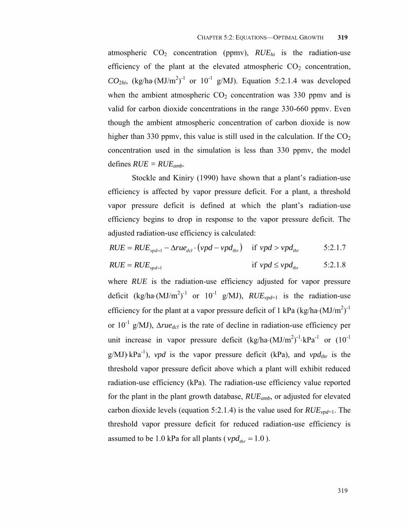
CHAPTER 5:2: EQUATIONS—OPTIMAL GROWTH
319
319
atmospheric CO2 concentration (ppmv), RUEhi is the radiation-use
efficiency of the plant at the elevated atmospheric CO2 concentration,
CO2hi, (kg/ha(MJ/m2)-1 or 10-1 g/MJ). Equation 5:2.1.4 was developed
when the ambient atmospheric CO2 concentration was 330 ppmv and is
valid for carbon dioxide concentrations in the range 330-660 ppmv. Even
though the ambient atmospheric concentration of carbon dioxide is now
higher than 330 ppmv, this value is still used in the calculation. If the CO2
concentration used in the simulation is less than 330 ppmv, the model
defines RUE = RUEamb.
Stockle and Kiniry (1990) have shown that a plant’s radiation-use
efficiency is affected by vapor pressure deficit. For a plant, a threshold
vapor pressure deficit is defined at which the plant’s radiation-use
efficiency begins to drop in response to the vapor pressure deficit. The
adjusted radiation-use efficiency is calculated:
thrdclvpd vpdvpdrueRUERUE 1 if thrvpdvpd 5:2.1.7
1 vpdRUERUE if thrvpdvpd 5:2.1.8
where RUE is the radiation-use efficiency adjusted for vapor pressure
deficit (kg/ha(MJ/m2)-1 or 10-1 g/MJ), RUEvpd=1 is the radiation-use
efficiency for the plant at a vapor pressure deficit of 1 kPa (kg/ha(MJ/m2)-1
or 10-1 g/MJ), ruedcl is the rate of decline in radiation-use efficiency per
unit increase in vapor pressure deficit (kg/ha(MJ/m2)-1kPa-1 or (10-1
g/MJ)kPa-1), vpd is the vapor pressure deficit (kPa), and vpdthr is the
threshold vapor pressure deficit above which a plant will exhibit reduced
radiation-use efficiency (kPa). The radiation-use efficiency value reported
for the plant in the plant growth database, RUEamb, or adjusted for elevated
carbon dioxide levels (equation 5:2.1.4) is the value used for RUEvpd=1. The
threshold vapor pressure deficit for reduced radiation-use efficiency is
assumed to be 1.0 kPa for all plants ( 0.1thrvpd ).

320 SWAT THEORETICAL DOCUMENTATION, VERSION 2009
320
The radiation-use efficiency is never allowed to fall below 27% of
RUEamb. This minimum value was based on field observations (Kiniry,
personal communication, 2001).
5:2.1.1.2 MODIFICATION OF BIOMASS CALCULATION FOR TREES With annuals and perennials, the plants are able to reach full
maturity within a single calendar year. With trees, a number of years are
needed for a plant to transition from a seedling to a sapling to a fully-
developed tree. The parameters in the plant growth database related to
radiation-use efficiency represent the annual growth for a fully-developed
tree. The heat units to maturity input in the management file is also used to
simulate growth within a single year, defining for trees and perennials the
period within a year bounded by the development of buds at the beginning
of the annual growing season and the maturation of plant seeds at the end
of the growing season.
To simulate the smaller amount of biomass accumulation seen in
seedlings/saplings, tree growth within a single year is limited to a fixed
amount determined by the age of the tree relative to the number of years for
the tree species to reach full development. Parameters in the plant growth
database define the total number of years for trees to reach full
development as well as the biomass of a fully-developed tree. Until the
trees in an HRU reach full development, the amount of biomass they can
accumulate in a single year is limited to:
fulldev
fulldev
cur
annual bioyr
yrbio
1000 5:2.1.9
where bioannual is the amount of biomass a tree can accumulate in a single
year (kg/ha), yrcur is the current age of the tree (years), yrfulldev is the number
of years for the tree species to reach full development (years), biofulldev is
the biomass of a fully developed tree stand for the specific tree species
(metric tons/ha), and 1000 is a conversion factor.

CHAPTER 5:2: EQUATIONS—OPTIMAL GROWTH
321
321
Once the total growth in biomass in a year, bio, reaches the annual
limit, biofulldev, no more growth occurs until the next year when a new
annual limit is calculated. When a tree stand has reached its biomass limit
in a year, the increase in plant biomass for a day, bioi, is set to 0.
5:2.1.2 CANOPY COVER AND HEIGHT
The change in canopy height and leaf area for annuals and perennials
through the growing season as modeled by SWAT is illustrated using parameters
for Alamo Switchgrass in Figures 5:2-1 and 5:2-2.
Figure 5:2-1: Seasonal change in annual/perennial plant canopy height during growing season.
Figure 5:2-2: Seasonal change in annual/perennial plant leaf area index during growing season.

322 SWAT THEORETICAL DOCUMENTATION, VERSION 2009
322
In the initial period of plant growth, canopy height and leaf area
development are controlled by the optimal leaf area development curve:
PHUPHU
PHULAImx
frfr
frfr
21exp 5:2.1.10
where frLAImx is the fraction of the plant’s maximum leaf area index corresponding
to a given fraction of potential heat units for the plant, frPHU is the fraction of
potential heat units accumulated for the plant on a given day in the growing
season, and 1 and 2 are shape coefficients. The fraction of potential heat units
accumulated by a given date is calculated:
PHU
HU
fr
d
i
i
PHU
1 5:2.1.11
where frPHU is the fraction of potential heat units accumulated for the plant on
day d in the growing season, HU is the heat units accumulated on day i (heat
units), and PHU is the total potential heat units for the plant (heat units).
The shape coefficients are calculated by solving equation 5:2.1.10 using
two known points (frLAI,1,frPHU,1) and (frLAI,2,frPHU,2):
1,21,1,
1,1 ln PHUPHU
LAI
PHUfrfr
fr
fr
5:2.1.12
1,2,
2,2,
2,1,
1,
1,
2
lnln
PHUPHU
PHU
LAI
PHU
PHU
LAI
PHU
frfr
frfr
frfr
fr
fr
5:2.1.13
where 1 is the first shape coefficient, 2 is the second shape coefficient, frPHU,1
is the fraction of the growing season (i.e. fraction of total potential heat units)
corresponding to the 1st point on the optimal leaf area development curve, frLAI,1 is
the fraction of the maximum plant leaf area index (i.e. fraction of LAImx)
corresponding to the 1st point on the optimal leaf area development curve, frPHU,2
is the fraction of the growing season corresponding to the 2nd point on the optimal
leaf area development curve, and frLAI,2 is the fraction of the maximum plant leaf
area index corresponding to the 2nd point on the optimal leaf area development
curve.

CHAPTER 5:2: EQUATIONS—OPTIMAL GROWTH
323
323
The canopy height on a given day is calculated:
LAImxmxcc frhh , 5:2.1.14
where hc is the canopy height for a given day (m), hc,mx is the plant’s maximum
canopy height (m), and frLAImx is the fraction of the plant’s maximum leaf area
index corresponding to a given fraction of potential heat units for the plant. As
can be seen from Figure 5:2-1, once the maximum canopy height is reached, hc
will remain constant until the plant is killed.
For tree stands, the canopy height varies from year to year rather than day
to day:
fulldev
cur
mxccyr
yrhh , 5:2.1.15
where hc is the canopy height for a given day (m), hc,mx is the plant’s maximum
canopy height (m), yrcur is the age of the tree (years), and yrfulldev is the number of
years for the tree species to reach full development (years).
The amount of canopy cover is expressed as the leaf area index. For
annuals and perennials, the leaf area added on day i is calculated:
mximxixLAiLAImxi LAILAILAIfrfrLAI 11,Im, 5exp1 5:2.1.16
while for trees, the leaf area added on day i is calculated:
mx
fulldev
cur
ixLAiLAImxi LAIyr
yrfrfrLAI 1,Im,
mx
fulldev
cur
i LAIyr
yrLAI 15exp1 5:2.1.17
The total leaf area index is calculated:
iii LAILAILAI 1 5:2.1.18
where LAIi is the leaf area added on day i, LAIi and LAIi-1 are the leaf area
indices for day i and i-1 respectiviely, frLAImx,i and frLAImx,i-1 are the fraction of the
plant’s maximum leaf area index calculated with equation 5:2.1.10 for day i and i-
1, LAImx is the maximum leaf area index for the plant, yrcur is the age of the tree

324 SWAT THEORETICAL DOCUMENTATION, VERSION 2009
324
(years), and yrfulldev is the number of years for the tree species to reach full
development (years).
Leaf area index is defined as the area of green leaf per unit area of land
(Watson, 1947). As shown in Figure 5:2-2, once the maximum leaf area index is
reached, LAI will remain constant until leaf senescence begins to exceed leaf
growth. Once leaf senescence becomes the dominant growth process, the leaf area
index for annuals and perrenials is calculated:
senPHU
PHUmx
fr
frLAILAI
,11
senPHUPHU frfr , 5:2.1.19
while for trees, the calculation is
senPHU
PHU
mx
fulldev
cur
fr
frLAI
yr
yrLAI
,11
senPHUPHU frfr , 5:2.1.20
where LAI is the leaf area index for a given day, LAImx is the maximum leaf area
index, frPHU is the fraction of potential heat units accumulated for the plant on a
given day in the growing season, frPHU,sen is the fraction of growing season (PHU)
at which senescence becomes the dominant growth process, yrcur is the number of
years of development the tree has accrued (years), and yrfulldev is the number of
years for the tree species to reach full development (years).
5:2.1.3 ROOT DEVELOPMENT The amount of total plant biomass partitioned to the root system is 30-50%
in seedlings and decreases to 5-20% in mature plants (Jones, 1985). SWAT varies
the fraction of total biomass in roots from 0.40 at emergence to 0.20 at maturity.
The daily root biomass fraction is calculated with the equation:
PHUroot frfr 20.040.0 5:2.1.21
where frroot is the fraction of total biomass partitioned to roots on a given day in
the growing season, and frPHU is the fraction of potential heat units accumulated
for the plant on a given day in the growing season.
Calculation of root depth varies according to plant type. SWAT assumes
perennials and trees have roots down to the maximum rooting depth defined for
the soil throughout the growing season:

CHAPTER 5:2: EQUATIONS—OPTIMAL GROWTH
325
325
mxrootroot zz , 5:2.1.22
where zroot is the depth of root development in the soil on a given day (mm), and
zroot,mx is the maximum depth for root development in the soil (mm). The
simulated root depth for annuals varies linearly from 10.0 mm at the beginning of
the growing season to the maximum rooting depth at frPHU = 0.40 using the
equation:
mxrootPHUroot zfrz ,5.2 if 40.0PHUfr 5:2.1.23
mxrootroot zz , if 40.0PHUfr 5:2.1.24
where zroot is the depth of root development in the soil on a given day (mm), frPHU
is the fraction of potential heat units accumulated for the plant on a given day in
the growing season, and zroot,mx is the maximum depth for root development in the
soil (mm). The maximum rooting depth is defined by comparing the maximum
potential rooting depth for the plant from the plant growth database (RDMX in
crop.dat), and the maximum potential rooting depth for the soil from the soil input
file (SOL_ZMX in .sol—if no value is provided for this variable the model will
set it to the deepest depth specified for the soil profile). The shallower of these
two depths is the value used for zroot,mx.
5:2.1.4 MATURITY
Plant maturity is reached when the fraction of potential heat units
accumulated, frPHU, is equal to 1.00. Once maturity is reached, the plant ceases to
transpire and take up water and nutrients. Simulated plant biomass remains stable
until the plant is harvested or killed via a management operation.
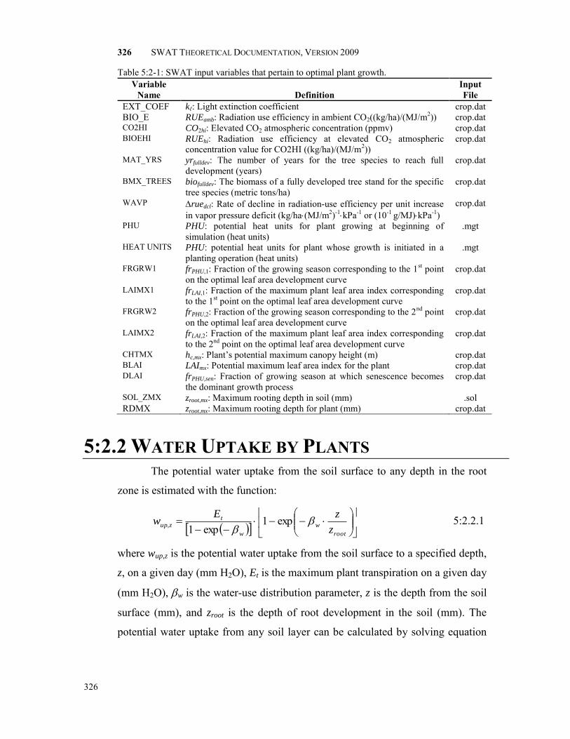
326 SWAT THEORETICAL DOCUMENTATION, VERSION 2009
326
Table 5:2-1: SWAT input variables that pertain to optimal plant growth. Variable
Name
Definition Input File
EXT_COEF kℓ: Light extinction coefficient crop.dat BIO_E RUEamb: Radiation use efficiency in ambient CO2((kg/ha)/(MJ/m2)) crop.dat CO2HI CO2hi: Elevated CO2 atmospheric concentration (ppmv) crop.dat BIOEHI RUEhi: Radiation use efficiency at elevated CO2 atmospheric
concentration value for CO2HI ((kg/ha)/(MJ/m2)) crop.dat
MAT_YRS yrfulldev: The number of years for the tree species to reach full development (years)
crop.dat
BMX_TREES biofulldev: The biomass of a fully developed tree stand for the specific tree species (metric tons/ha)
crop.dat
WAVP ruedcl: Rate of decline in radiation-use efficiency per unit increase in vapor pressure deficit (kg/ha(MJ/m2)-1
kPa-1 or (10-1 g/MJ)kPa-1) crop.dat
PHU PHU: potential heat units for plant growing at beginning of simulation (heat units)
.mgt
HEAT UNITS PHU: potential heat units for plant whose growth is initiated in a planting operation (heat units)
.mgt
FRGRW1 frPHU,1: Fraction of the growing season corresponding to the 1st point on the optimal leaf area development curve
crop.dat
LAIMX1 frLAI,1: Fraction of the maximum plant leaf area index corresponding to the 1st point on the optimal leaf area development curve
crop.dat
FRGRW2 frPHU,2: Fraction of the growing season corresponding to the 2nd point on the optimal leaf area development curve
crop.dat
LAIMX2 frLAI,2: Fraction of the maximum plant leaf area index corresponding to the 2nd point on the optimal leaf area development curve
crop.dat
CHTMX hc,mx: Plant’s potential maximum canopy height (m) crop.dat BLAI LAImx: Potential maximum leaf area index for the plant crop.dat DLAI frPHU,sen: Fraction of growing season at which senescence becomes
the dominant growth process crop.dat
SOL_ZMX zroot,mx: Maximum rooting depth in soil (mm) .sol RDMX zroot,mx: Maximum rooting depth for plant (mm) crop.dat
5:2.2 WATER UPTAKE BY PLANTS The potential water uptake from the soil surface to any depth in the root
zone is estimated with the function:
root
w
w
tzup
z
zEw
exp1
exp1, 5:2.2.1
where wup,z is the potential water uptake from the soil surface to a specified depth,
z, on a given day (mm H2O), Et is the maximum plant transpiration on a given day
(mm H2O), w is the water-use distribution parameter, z is the depth from the soil
surface (mm), and zroot is the depth of root development in the soil (mm). The
potential water uptake from any soil layer can be calculated by solving equation

CHAPTER 5:2: EQUATIONS—OPTIMAL GROWTH
327
327
5:2.2.1 for the depth at the top and bottom of the soil layer and taking the
difference.
zuupzluplyup www ,,, 5:2.2.2
where wup,ly is the potential water uptake for layer ly (mm H2O), wup,zl is the
potential water uptake for the profile to the lower boundary of the soil layer (mm
H2O), and wup,zu is the potential water uptake for the profile to the upper boundary
of the soil layer (mm H2O).
Since root density is greatest near the soil surface and decreases with
depth, the water uptake from the upper layers is assumed to be much greater than
that in the lower layers. The water-use distribution parameter, w, is set to 10 in
SWAT. With this value, 50% of the water uptake will occur in the upper 6% of
the root zone. Figure 5:2-3 graphically displays the uptake of water at different
depths in the root zone.
Figure 5:2-3: Depth distribution of water uptake

328 SWAT THEORETICAL DOCUMENTATION, VERSION 2009
328
The amount of water uptake that occurs on a given day is a function of the amount
of water required by the plant for transpiration, Et, and the amount of water
available in the soil, SW. Equations 5:2.2.1 and 5:2.2.2 calculate potential water
uptake solely as a function of water demand for transpiration and the depth
distribution defined in equation 5:2.2.1. SWAT modifies the initial potential water
uptake from a given soil layer to reflect soil water availability in the following
ways.
5:2.2.1 IMPACT OF LOW SOIL WATER CONTENT
If upper layers in the soil profile do not contain enough water to meet the
potential water uptake calculated with equation 5:2.2.2, users may allow lower
layers to compensate. The equation used to calculate the adjusted potential water
uptake is:
epcowww demandlyuplyup ,, 5:2.2.3
where lyupw , is the adjusted potential water uptake for layer ly (mm H2O), wup,ly is
the potential water uptake for layer ly calculated with equation 5:2.2.2 (mm H2O),
wdemand is the water uptake demand not met by overlying soil layers (mm H2O),
and epco is the plant uptake compensation factor. The plant uptake compensation
factor can range from 0.01 to 1.00 and is set by the user. As epco approaches 1.0,
the model allows more of the water uptake demand to be met by lower layers in
the soil. As epco approaches 0.0, the model allows less variation from the depth
distribution described by equation 5:2.2.1 to take place.
As the water content of the soil decreases, the water in the soil is held
more and more tightly by the soil particles and it becomes increasingly difficult
for the plant to extract water from the soil. To reflect the decrease in the
efficiency of the plant in extracting water from dryer soils, the potential water
uptake is modified using the following equations:
1
25.5exp,,
ly
ly
lyuplyupAWC
SWww when
lyly AWCSW 25. 5:2.2.4
lyuplyup ww ,, when lyly AWCSW 25. 5:2.2.5

CHAPTER 5:2: EQUATIONS—OPTIMAL GROWTH
329
329
where lyupw , is the potential water uptake adjusted for initial soil water content
(mm H2O), lyupw , is the adjusted potential water uptake for layer ly (mm H2O),
SWly is the amount of water in the soil layer on a given day (mm H2O), and AWCly
is the available water capacity for layer ly (mm H2O). The available water
capacity is calculated:
lylyly WPFCAWC 5:2.2.6
where AWCly is the available water capacity for layer ly (mm H2O), FCly is the
water content of layer ly at field capacity (mm H2O), and WPly is the water
content of layer ly at wilting point (mm H2O).
5:2.2.2 ACTUAL WATER UPTAKE
Once the potential water uptake has been modified for soil water
conditions, the actual amount of water uptake from the soil layer is calculated:
lylylyuplyactualup WPSWww ,min ,, 5:2.2.7
where wactualup,ly is the actual water uptake for layer ly (mm H2O), SWly is the
amount of water in the soil layer on a given day (mm H2O), and WPly is the water
content of layer ly at wilting point (mm H2O). The total water uptake for the day
is calculated:
n
ly
lyactualupactualup ww1
, 5:2.2.8
where wactualup is the total plant water uptake for the day (mm H2O), wactualup,ly is
the actual water uptake for layer ly (mm H2O), and n is the number of layers in the
soil profile. The total plant water uptake for the day calculated with equation
5:2.2.8 is also the actual amount of transpiration that occurs on the day.
actualupactt wE , 5:2.2.9
where Et,act is the actual amount of transpiration on a given day (mm H2O) and
wactualup is the total plant water uptake for the day (mm H2O).
Table 5:2-2: SWAT input variables that pertain to plant water uptake. Variable
Name
Definition Input File
EPCO epco: Plant uptake compensation factor .bsn, .hru

330 SWAT THEORETICAL DOCUMENTATION, VERSION 2009
330
5:2.3 NUTRIENT UPTAKE BY PLANTS SWAT monitors plant uptake of nitrogen and phosphorus.
5:2.3.1 NITROGEN UPTAKE Plant nitrogen uptake is controlled by the plant nitrogen equation. The
plant nitrogen equation calculates the fraction of nitrogen in the plant biomass as
a function of growth stage given optimal growing conditions.
3,
213,1, exp
1 N
PHUPHU
PHUNNN fr
frnnfr
frfrfrfr
5:2.3.1
where frN is the fraction of nitrogen in the plant biomass on a given day, frN,1 is
the normal fraction of nitrogen in the plant biomass at emergence, frN,3 is the
normal fraction of nitrogen in the plant biomass at maturity, frPHU is the fraction
of potential heat units accumulated for the plant on a given day in the growing
season, and n1 and n2 are shape coefficients.
The shape coefficients are calculated by solving equation 5:2.3.1 using
two known points (frN,2, frPHU,50%) and (frN,3, frPHU,100%):
%50,2%50,
3,1,
3,2,
%50,1
1ln PHUPHU
NN
NN
PHUfrnfr
frfr
frfr
frn
5:2.3.2
%50,%100,
%100,
3,1,
3,3~,
%100,%50,
3,1,
3,2,
%50,
2
1ln
1ln
PHUPHU
PHU
NN
NN
PHU
PHU
NN
NN
PHU
frfr
fr
frfr
frfr
frfr
frfr
frfr
fr
n
5:2.3.3
where n1 is the first shape coefficient, n2 is the second shape coefficient, frN,1 is
the normal fraction of nitrogen in the plant biomass at emergence, frN,2 is the
normal fraction of nitrogen in the plant biomass at 50% maturity, frN,3 is the
normal fraction of nitrogen in the plant biomass at maturity, frN,~3 is the normal
fraction of nitrogen in the plant biomass near maturity, frPHU,50% is the fraction of
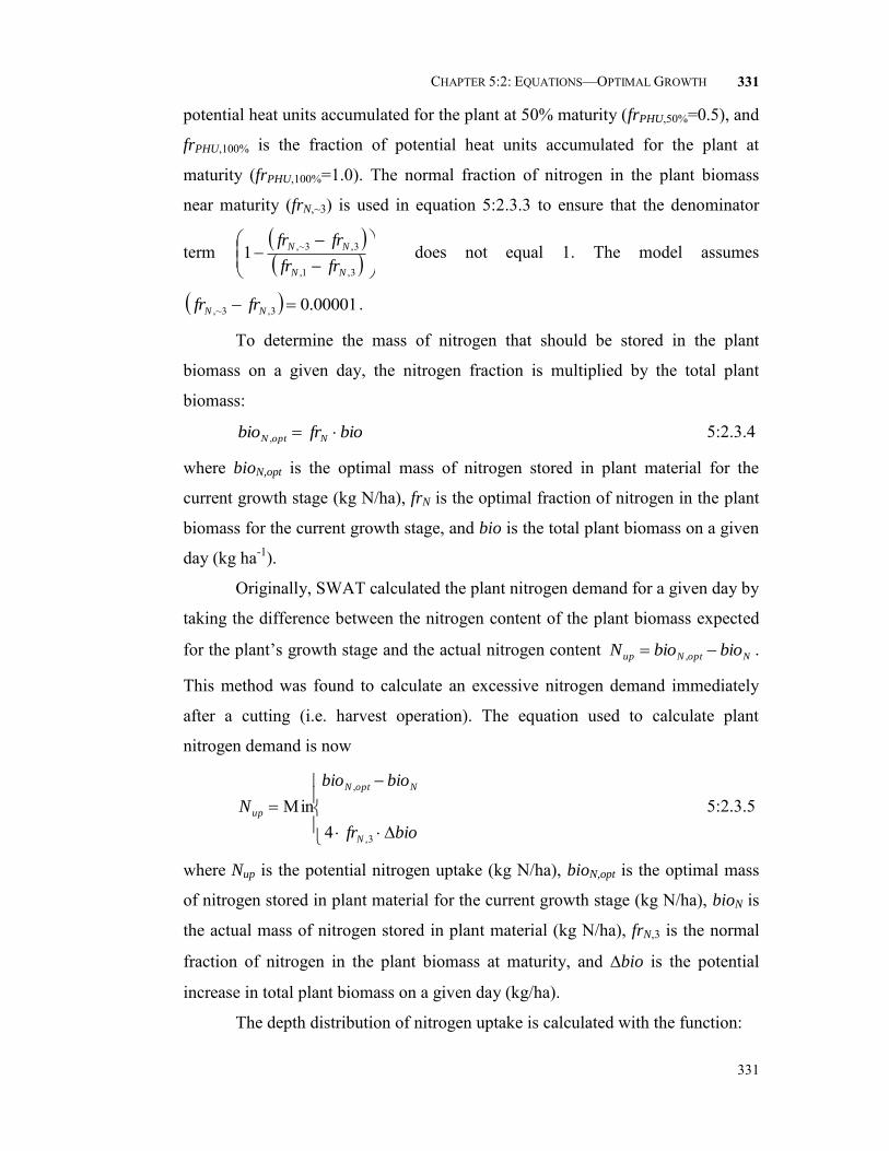
CHAPTER 5:2: EQUATIONS—OPTIMAL GROWTH
331
331
potential heat units accumulated for the plant at 50% maturity (frPHU,50%=0.5), and
frPHU,100% is the fraction of potential heat units accumulated for the plant at
maturity (frPHU,100%=1.0). The normal fraction of nitrogen in the plant biomass
near maturity (frN,~3) is used in equation 5:2.3.3 to ensure that the denominator
term
3,1,
3,3~,1NN
NN
frfr
frfr does not equal 1. The model assumes
00001.03,3~, NN frfr .
To determine the mass of nitrogen that should be stored in the plant
biomass on a given day, the nitrogen fraction is multiplied by the total plant
biomass:
biofrbio NoptN , 5:2.3.4
where bioN,opt is the optimal mass of nitrogen stored in plant material for the
current growth stage (kg N/ha), frN is the optimal fraction of nitrogen in the plant
biomass for the current growth stage, and bio is the total plant biomass on a given
day (kg ha-1).
Originally, SWAT calculated the plant nitrogen demand for a given day by
taking the difference between the nitrogen content of the plant biomass expected
for the plant’s growth stage and the actual nitrogen content NoptNup biobioN , .
This method was found to calculate an excessive nitrogen demand immediately
after a cutting (i.e. harvest operation). The equation used to calculate plant
nitrogen demand is now
biofr
biobio
N
N
NoptN
up
3,
,
4Min 5:2.3.5
where Nup is the potential nitrogen uptake (kg N/ha), bioN,opt is the optimal mass
of nitrogen stored in plant material for the current growth stage (kg N/ha), bioN is
the actual mass of nitrogen stored in plant material (kg N/ha), frN,3 is the normal
fraction of nitrogen in the plant biomass at maturity, and bio is the potential
increase in total plant biomass on a given day (kg/ha).
The depth distribution of nitrogen uptake is calculated with the function:

332 SWAT THEORETICAL DOCUMENTATION, VERSION 2009
332
root
n
n
up
zupz
zNN
exp1
exp1, 5:2.3.6
where Nup,z is the potential nitrogen uptake from the soil surface to depth z (kg
N/ha), Nup is the potential nitrogen uptake (kg N/ha), n is the nitrogen uptake
distribution parameter, z is the depth from the soil surface (mm), and zroot is the
depth of root development in the soil (mm). Note that equation 5:2.3.6 is similar
in form to the depth distribution for water uptake described by equation 5:2.2.1.
The potential nitrogen uptake for a soil layer is calculated by solving equation
5:2.3.6 for the depth at the upper and lower boundaries of the soil layer and taking
the difference.
zuupzluplyup NNN ,,, 5:2.3.7
where Nup,ly is the potential nitrogen uptake for layer ly (kg N/ha), Nup,zl is the
potential nitrogen uptake from the soil surface to the lower boundary of the soil
layer (kg N/ha), and Nup,zu is the potential nitrogen uptake from the soil surface to
the upper boundary of the soil layer (kg N/ha).
Root density is greatest near the surface, and nitrogen uptake in the upper
portion of the soil will be greater than in the lower portion. The depth distribution
of nitrogen uptake is controlled by n, the nitrogen uptake distribution parameter,
a variable users are allowed to adjust. Figure 5:2-4 illustrates nitrogen uptake as a
function of depth for four different uptake distribution parameter values.
Nitrogen removed from the soil by plants is taken from the nitrate pool.
The importance of the nitrogen uptake distribution parameter lies in its control
over the maximum amount of nitrate removed from the upper layers. Because the
top 10 mm of the soil profile interacts with surface runoff, the nitrogen uptake
distribution parameter will influence the amount of nitrate available for transport
in surface runoff. The model allows lower layers in the root zone to fully
compensate for lack of nitrate in the upper layers, so there should not be
significant changes in nitrogen stress with variation in the value used for n.
The actual amount if nitrogen removed from a soil layer is calculated:
lydemandlyuplyactualup NO3NNN ,min ,, 5:2.3.8

CHAPTER 5:2: EQUATIONS—OPTIMAL GROWTH
333
333
where Nactualup,ly is the actual nitrogen uptake for layer ly (kg N/ha), Nup,ly is the
potential nitrogen uptake for layer ly (kg N/ha), Ndemand is the nitrogen uptake
demand not met by overlying soil layers (kg N/ha), and NO3ly is the nitrate
content of soil layer ly (kg NO3-N/ha).
Figure 5:2-4: Depth distribution of nitrogen uptake
5:2.3.1.1 NITROGEN FIXATION If nitrate levels in the root zone are insufficient to meet the demand
of a legume, SWAT allows the plant to obtain additional nitrogen through
nitrogen fixation. Nitrogen fixation is calculated as a function of soil
water, soil nitrate content and growth stage of the plant.
1,,min 3noswgrdemandfix fffNN 5:2.3.9
where Nfix is the amount of nitrogen added to the plant biomass by fixation
(kg N/ha), Ndemand is the plant nitrogen demand not met by uptake from the
soil (kg N/ha), fgr is the growth stage factor (0.0-1.0), fsw is the soil water

334 SWAT THEORETICAL DOCUMENTATION, VERSION 2009
334
factor (0.0-1.0), and fno3 is the soil nitrate factor (0.0-1.0). The maximum
amount of nitrogen that can be fixed by the plant on a given day is Ndemand.
Growth stage exerts the greatest impact on the ability of the plant
to fix nitrogen. The growth stage factor is calculated:
0grf when 15.0PHUfr 5:2.3.10
167.6 PHUgr frf when 30.015.0 PHUfr 5:2.3.11
1grf when 55.030.0 PHUfr 5:2.3.12
PHUgr frf 575.3 when 75.055.0 PHUfr 5:2.3.13
0grf when 75.0PHUfr 5:2.3.14
where fgr is the growth stage factor and frPHU is the fraction of potential
heat units accumulated for the plant on a given day in the growing season.
The growth stage factor is designed to reflect the buildup and decline of
nitrogen fixing bacteria in the plant roots during the growing season.
The soil nitrate factor inhibits nitrogen fixation as the presence of
nitrate in the soil goes up. The soil nitrate factor is calculated:
13 nof when 1003 NO 5:2.3.15
30005.05.13 NOfno when 3003100 NO 5:2.3.16
03 nof when 3003 NO 5:2.3.17
where fno3 is the soil nitrate factor and NO3 is the nitrate content of the soil
profile (kg NO3-N/ha).
The soil water factor inhibits nitrogen fixation as the soil dries out.
The soil water factor is calculated:
FC
SWf sw
85. 5:2.3.18
where fsw is the soil water factor, SW is the amount of water in soil profile
(mm H2O), and FC is the water content of soil profile at field capacity
(mm H2O).

CHAPTER 5:2: EQUATIONS—OPTIMAL GROWTH
335
335
5:2.3.2 PHOSPHORUS UPTAKE Plant phosphorus uptake is controlled by the plant phosphorus equation.
The plant phosphorus equation calculates the fraction of phosphorus in the plant
biomass as a function of growth stage given optimal growing conditions.
3,
213,1, exp
1 P
PHUPHU
PHUPPP fr
frppfr
frfrfrfr
5:2.3.19
where frP is the fraction of phosphorus in the plant biomass on a given day, frP,1 is
the normal fraction of phosphorus in the plant biomass at emergence, frP,3 is the
normal fraction of phosphorus in the plant biomass at maturity, frPHU is the
fraction of potential heat units accumulated for the plant on a given day in the
growing season, and p1 and p2 are shape coefficients.
The shape coefficients are calculated by solving equation 5:2.3.19 using
two known points (frP,2, frPHU,50%) and (frP,3, frPHU,100%):
%50,2%50,
3,1,
3,2,
%50,1
1ln PHUPHU
PP
PP
PHUfrpfr
frfr
frfr
frp
5:2.3.20
%50,%100,
%100,
3,1,
3,3~,
%100,%50,
3,1,
3,2,
%50,
2
1ln
1ln
PHUPHU
PHU
PP
PP
PHU
PHU
PP
PP
PHU
frfr
fr
frfr
frfr
frfr
frfr
frfr
fr
p
5:2.3.21
where p1 is the first shape coefficient, p2 is the second shape coefficient, frP,1 is
the normal fraction of phosphorus in the plant biomass at emergence, frP,2 is the
normal fraction of phosphorus in the plant biomass at 50% maturity, frP,3 is the
normal fraction of phosphorus in the plant biomass at maturity, frP,~3 is the normal
fraction of phosphorus in the plant biomass near maturity, frPHU,50% is the fraction
of potential heat units accumulated for the plant at 50% maturity (frPHU,50%=0.5),
and frPHU,100% is the fraction of potential heat units accumulated for the plant at
maturity (frPHU,100%=1.0). The normal fraction of phosphorus in the plant biomass

336 SWAT THEORETICAL DOCUMENTATION, VERSION 2009
336
near maturity (frN,~3) is used in equation 5:2.3.21 to ensure that the denominator
term
3,1,
3,3~,1PP
PP
frfr
frfr does not equal 1. The model assumes
00001.03,3~, PP frfr .
To determine the mass of phosphorus that should be stored in the plant
biomass for the growth stage, the phosphorus fraction is multiplied by the total
plant biomass:
biofrbio PoptP , 5:2.3.22
where bioP,opt is the optimal mass of phosphorus stored in plant material for the
current growth stage (kg P/ha), frP is the optimal fraction of phophorus in the
plant biomass for the current growth stage, and bio is the total plant biomass on a
given day (kg ha-1).
Originally, SWAT calculated the plant nutrient demand for a given day by
taking the difference between the nutrient content of the plant biomass expected
for the plant’s growth stage and the actual nutrient content. This method was
found to calculate an excessive nutrient demand immediately after a cutting (i.e.
harvest operation). The plant phosphorus demand for a given day is calculated:
biofr
biobioP
P
PoptP
up
3,
,
4Min5.1 5:2.3.23
where Pup is the potential phosphorus uptake (kg P/ha), bioP,opt is the optimal mass
of phosphorus stored in plant material for the current growth stage (kg P/ha), and
bioP is the actual mass of phosphorus stored in plant material (kg P/ha), frP,3 is the
normal fraction of phosphorus in the plant biomass at maturity, and bio is the
potential increase in total plant biomass on a given day (kg/ha). The difference
between the phosphorus content of the plant biomass expected for the plant’s
growth stage and the actual phosphorus content is multiplied by 1.5 to simulate
luxury phosphorus uptake.
The depth distribution of phosphorus uptake is calculated with the
function:

CHAPTER 5:2: EQUATIONS—OPTIMAL GROWTH
337
337
root
p
p
up
zupz
zPP
exp1
exp1, 5:2.3.24
where Pup,z is the potential phosphorus uptake from the soil surface to depth z (kg
P/ha), Pup is the potential phosphorus uptake (kg P/ha), P is the phosphorus
uptake distribution parameter, z is the depth from the soil surface (mm), and zroot
is the depth of root development in the soil (mm). The potential phosphorus
uptake for a soil layer is calculated by solving equation 5:2.3.24 for the depth at
the upper and lower boundaries of the soil layer and taking the difference.
zuupzluplyup PPP ,,, 5:2.3.25
where Pup,ly is the potential phosphorus uptake for layer ly (kg P/ha), Pup,zl is the
potential phosphorus uptake from the soil surface to the lower boundary of the
soil layer (kg P/ha), and Pup,zu is the potential phosphorus uptake from the soil
surface to the upper boundary of the soil layer (kg P/ha).
Root density is greatest near the surface, and phosphorus uptake in the
upper portion of the soil will be greater than in the lower portion. The depth
distribution of phosphorus uptake is controlled by p, the phosphorus uptake
distribution parameter, a variable users are allowed to adjust. The illustration of
nitrogen uptake as a function of depth for four different uptake distribution
parameter values in Figure 5:2-4 is valid for phosphorus uptake as well.
Phosphorus removed from the soil by plants is taken from the solution
phosphorus pool. The importance of the phosphorus uptake distribution parameter
lies in its control over the maximum amount of solution P removed from the
upper layers. Because the top 10 mm of the soil profile interacts with surface
runoff, the phosphorus uptake distribution parameter will influence the amount of
labile phosphorus available for transport in surface runoff. The model allows
lower layers in the root zone to fully compensate for lack of solution P in the
upper layers, so there should not be significant changes in phosphorus stress with
variation in the value used for p.
The actual amount if phosphorus removed from a soil layer is calculated:
lysolutiondemandlyuplyactualup PPPP ,,, ,min 5:2.3.26

338 SWAT THEORETICAL DOCUMENTATION, VERSION 2009
338
where Pactualup,ly is the actual phosphorus uptake for layer ly (kg P/ha), Pup,ly is the
potential phosphorus uptake for layer ly (kg P/ha), Pdemand is the phosphorus
uptake demand not met by overlying soil layers (kg P/ha), and Psolution,ly is the
phosphorus content of the soil solution in layer ly (kg P/ha).
Table 5:2-3: SWAT input variables that pertain to plant nutrient uptake. Variable
Name
Definition Input File
PLTNFR(1) frN,1: Normal fraction of N in the plant biomass at emergence crop.dat PLTNFR(2) frN,2: Normal fraction of N in the plant biomass at 50% maturity crop.dat PLTNFR(3) frN,3: Normal fraction of N in the plant biomass at maturity crop.dat N_UPDIS n: Nitrogen uptake distribution parameter .bsn PLTPFR(1) frP,1: Normal fraction of P in the plant biomass at emergence crop.dat PLTPFR(2) frP,2: Normal fraction of P in the plant biomass at 50% maturity crop.dat PLTPFR(3) frP,3: Normal fraction of P in the plant biomass at maturity crop.dat P_UPDIS p: Phosphorus uptake distribution parameter .bsn
5:2.4 CROP YIELD When a harvest or harvest/kill operation is performed, a portion of the
plant biomass is removed from the HRU as yield. The nutrients and plant material
contained in the yield are assumed to be lost from the system (i.e. the watershed)
and will not be added to residue and organic nutrient pools in the soil with the
remainder of the plant material. In contrast, a kill operation converts all biomass
to residue.
The fraction of the above-ground plant dry biomass removed as dry
economic yield is called the harvest index. For the majority of crops, the harvest
index will be between 0.0 and 1.0. However, plants whose roots are harvested,
such as sweet potatoes, may have a harvest index greater than 1.0.
The economic yield of most commercial crops is the reproductive portion
of the plant. Decades of crop breeding have lead to cultivars and hybrids having
maximized harvest indices. Often, the harvest index is relatively stable across a
range of environmental conditions.
SWAT calculates harvest index each day of the plant’s growing season
using the relationship:
PHUPHU
PHUopt
frfr
frHIHI
101.11exp100100 5:2.4.1

CHAPTER 5:2: EQUATIONS—OPTIMAL GROWTH
339
339
where HI is the potential harvest index for a given day, HIopt is the potential
harvest index for the plant at maturity given ideal growing conditions, and frPHU is
the fraction of potential heat units accumulated for the plant on a given day in the
growing season. The variation of the optimal harvest index during the growing
season is illustrated in Figure 5:2-5.
The crop yield is calculated as:
HIbioyld ag when 00.1HI 5:2.4.2
HIbioyld
111 when 00.1HI 5:2.4.3
where yld is the crop yield (kg/ha), bioag is the aboveground biomass on the day
of harvest (kg ha-1), HI is the harvest index on the day of harvest, and bio is the
total plant biomass on the day of harvest (kg ha-1). The aboveground biomass is
calculated:
biofrbio rootag 1 5:2.4.4
where frroot is the fraction of total biomass in the roots the day of harvest, and bio
is the total plant biomass on the day of harvest (kg ha-1).
Figure 5:2-5: Variation in optimal harvest index (HIi/HIopt) with fraction of growing season (frPHU)
The amount of nutrients removed in the yield are calculated:
yldfryld yldNN , 5:2.4.5

340 SWAT THEORETICAL DOCUMENTATION, VERSION 2009
340
yldfryld yldPP , 5:2.4.6
where yldN is the amount of nitrogen removed in the yield (kg N/ha), yldP is the
amount of phosphorus removed in the yield (kg P/ha), frN,yld is the fraction of
nitrogen in the yield, frP,yld is the fraction of phosphorus in the yield, and yld is the
crop yield (kg/ha).
If the harvest index override is used in the harvest only operation, the
model assumes that a significant portion of the plant biomass is being removed in
addition to the seed. Therefore, instead of using the nitrogen and phosphorus yield
fractions from the plant growth database, the model uses the total biomass
nitrogen and phosphorus fractions to determine the amount of nitrogen and
phosphorus removed:
yldfryld NN 5:2.4.7
yldfryld PP 5:2.4.8
where yldN is the amount of nitrogen removed in the yield (kg N/ha), yldP is the
amount of phosphorus removed in the yield (kg P/ha), frN is the fraction of
nitrogen in the plant biomass calculated with equation 5:2.3.1, frP is the fraction
of phosphorus in the plant biomass calculated with equation 5:2.3.19, and yld is
the crop yield (kg/ha).
Table 5:2-4: SWAT input variables that pertain to crop yield. Variable
Name
Definition Input File
HVSTI HIopt: Potential harvest index for the plant at maturity given ideal growing conditions
crop.dat
CNYLD frN,yld: Fraction of nitrogen in the yield crop.dat CPYLD frP,yld: Fraction of phosphorus in the yield crop.dat
5:2.5 NOMENCLATURE AWCly Available water capacity for layer ly (mm H2O) CO2 Concentration of carbon dioxide in the atmosphere (ppmv) CO2amb Ambient atmospheric CO2 concentration (330 ppmv) CO2hi Elevated atmospheric CO2 concentration (ppmv) Et Maximum transpiration rate (mm d-1) Et,act Actual amount of transpiration on a given day (mm H2O) FC Water content of soil profile at field capacity (mm H2O)

CHAPTER 5:2: EQUATIONS—OPTIMAL GROWTH
341
341
FCly Water content of layer ly at field capacity (mm H2O) Hday Solar radiation reaching ground on current day of simulation (MJ m-2 d-1) Hphosyn Intercepted photosynthetically active radiation on a given day (MJ m-2) HI Potential harvest index for a given day HIopt Potential harvest index for the plant at maturity given ideal growing conditions
HU Number of heat units accumulated on a given day (heat units) LAI Leaf area index of the canopy
LAImx Maximum leaf area index for the plant Nactualup,ly Actual nitrogen uptake for layer ly (kg N/ha) Ndemand Nitrogen uptake demand not met by overlying soil layers (kg N/ha) Nfix Amount of nitrogen added to the plant biomass by fixation (kg N/ha) Nup Potential nitrogen uptake (kg N/ha) Nup,ly Potential nitrogen uptake for layer ly (kg N/ha) Nup,z Potential nitrogen uptake from the soil surface to depth z (kg N/ha) Nup,zl Potential nitrogen uptake from the soil surface to the lower boundary of the soil
layer (kg N/ha) Nup,zu Potential nitrogen uptake from the soil surface to the upper boundary of the soil
layer (kg N/ha) NO3 Nitrate content of the soil profile (kg NO3-N/ha) NO3ly Nitrate content of soil layer ly (kg NO3-N/ha) Pactualup,ly Actual phosphorus uptake for layer ly (kg P/ha) Pdemand Phosphorus uptake demand not met by overlying soil layers (kg P/ha) Pup Potential phosphorus uptake (kg P/ha) Pup,ly Potential phosphorus uptake for layer ly (kg P/ha) Pup,z Potential phosphorus uptake from the soil surface to depth z (kg P/ha) Pup,zl Potential phosphorus uptake from the soil surface to the lower boundary of the
soil layer (kg P/ha) Pup,zu Potential phosphorus uptake from the soil surface to the upper boundary of the
soil layer (kg P/ha) PHU Potential heat units or total heat units required for plant maturity (heat units) Psolution,ly Phosphorus content of soil solution in layer ly (kg P/ha) RUE Radiation-use efficiency of the plant (kg/ha(MJ/m2)-1 or 10-1 g/MJ) RUEamb Radiation-use efficiency of the plant at ambient atmospheric CO2 concentration
(kg/ha(MJ/m2)-1 or 10-1 g/MJ) RUEhi Radiation-use efficiency of the plant at the elevated atmospheric CO2
concentration, CO2hi, (kg/ha(MJ/m2)-1 or 10-1 g/MJ) RUEvpd=1 Radiation-use efficiency for the plant at a vapor pressure deficit of 1 kPa
(kg/ha(MJ/m2)-1 or 10-1 g/MJ) SAT Amount of water in the soil profile when completely saturated (mm H2O), SW Amount of water in soil profile (mm H2O) SWly Soil water content of layer ly (mm H2O) WPly Water content of layer ly at wilting point (mm H2O).
bio Total plant biomass on a given day (kg/ha) bioag Aboveground biomass on the day of harvest (kg ha-1) bioannual The amount of biomass a tree can accumulate in a single year (kg/ha)

342 SWAT THEORETICAL DOCUMENTATION, VERSION 2009
342
biofulldev The biomass of a fully developed tree for the specific tree species (metric tons/ha)
bioN Actual mass of nitrogen stored in plant material (kg N/ha) bioN,opt Optimal mass of nitrogen stored in plant material for the growth stage (kg N/ha) bioP Actual mass of phosphorus stored in plant material (kg P/ha) bioP,opt Optimal mass of phosphorus stored in plant material for the current growth stage
(kg P/ha) epco Plant uptake compensation factor fgr Growth stage factor in nitrogen fixation equation fno3 Soil nitrate factor in nitrogen fixation equation
fsw Soil water factor in nitrogen fixation equation frLAI,1 Fraction of the maximum plant leaf area index corresponding to the 1st point on
the optimal leaf area development curve
frLAI,2 Fraction of the maximum plant leaf area index corresponding to the 2nd point on the optimal leaf area development curve
frLAImx Fraction of the plant’s maximum leaf area index corresponding to a given fraction of potential heat units for the plant
frN Optimal fraction of nitrogen in the plant biomass for current growth stage frN,1 Normal fraction of nitrogen in the plant biomass at emergence frN,2 Normal fraction of nitrogen in the plant biomass at 50% maturity frN,3 Normal fraction of nitrogen in the plant biomass at maturity
frN,~3 Normal fraction of nitrogen in the plant biomass near maturity
frN,yld Fraction of nitrogen in the yield frP Fraction of phosphorus in the plant biomass frP,1 Normal fraction of phosphorus in the plant biomass at emergence frP,2 Normal fraction of phosphorus in the plant biomass at 50% maturity frP,3 Normal fraction of phosphorus in the plant biomass at maturity
frP,~3 Normal fraction of phosphorus in the plant biomass near maturity frP,yld Fraction of phosphorus in the yield
frPHU Fraction of potential heat units accumulated for the plant on a given day in the growing season
frPHU,1 Fraction of the growing season corresponding to the 1st point on the optimal leaf area development curve
frPHU,2 Fraction of the growing season corresponding to the 2nd point on the optimal leaf area development curve
frPHU,50% Fraction of potential heat units accumulated for the plant at 50% maturity (frPHU,50%=0.5)
frPHU,100% Fraction of potential heat units accumulated for the plant at maturity (frPHU,100%=1.0)
frPHU,sen Fraction of growing season at which senescence becomes the dominant growth process
frroot Fraction of total biomass in the roots on a given day in the growing season
hc Canopy height (cm) hc,mx Plant’s maximum canopy height (m)
k Light extinction coefficient n1 First shape coefficient in plant nitrogen equation

CHAPTER 5:2: EQUATIONS—OPTIMAL GROWTH
343
343
n2 Second shape coefficient in plant nitrogen equation
p1 First shape coefficient in plant phosphorus equation p2 Second shape coefficient in plant phosphorus equation
r1 First shape coefficient for radiation-use efficiency curve r2 Second shape coefficient for radiation-use efficiency curve vpd Vapor pressure deficit (kPa) vpdthr Threshold vapor pressure deficit above which a plant will exhibit reduced
radiation-use efficiency (kPa) wactualup Total plant water uptake for the day (mm H2O) wactualup,ly Actual water uptake for layer ly (mm H2O) wdemand Water uptake demand not met by overlying soil layers (mm H2O) wup,ly Potential water uptake for layer ly (mm H2O)
lyupw , Adjusted potential water uptake for layer ly (mm H2O)
lyupw , Potential water uptake when the soil water content is less than 25% of plant available water (mm H2O)
wup,z Potential water uptake from the soil surface to a specified depth, z, on a given day (mm H2O)
wup,zl is the potential water uptake for the profile to the lower boundary of the soil layer (mm H2O)
wup,zu is the potential water uptake for the profile to the upper boundary of the soil layer (mm H2O)
yld Crop yield (kg/ha) yldN Amount of nitrogen removed in the yield (kg N/ha) yldP Amount of phosphorus removed in the yield (kg P/ha) yrcur The number of years of development the tree has accrued (years) yrfulldev The number of years for the tree species to reach full development (years) z Depth below soil surface (mm) zroot Depth of root development in the soil (mm) zroot,mx Maximum depth for root development in the soil (mm)
n Nitrogen uptake distribution parameter p Phosphorus uptake distribution parameter w Water-use distribution parameter LAIi Leaf area added on day i bio Potential increase in total plant biomass on a given day (kg/ha) ruedcl Rate of decline in radiation-use efficiency per unit increase in vapor pressure
deficit (kg/ha(MJ/m2)-1kPa-1 or (10-1 g/MJ)kPa-1)
1 First shape coefficient for optimal leaf area development curve
2 Second shape coefficient for optimal leaf area development curve
344 SWAT THEORETICAL DOCUMENTATION, VERSION 2009
344
5:2.6 REFERENCES
Jones, C.A. 1985. C-4 grasses and cereals. John Wiley & Sons, Inc., New York.
419 pp.
McCree, K.J. 1972. The action spectrum, absorption and quantum yield of
photosynthesis in crop plants. Agric. Met. 9:191-216.
Monsi, M. and T. Saeki. 1953. Uber den Lictfaktor in den Pflanzengesellschaften
und sein Bedeutung fur die Stoffproduktion. Japan J. Bot. 14:22-52.
Monteith, J.L. 1972. Solar radiation and productivity in tropical ecosystems. J.
Appl. Ecol. 9:747-766.
Monteith, J.L. 1977. Climate and the efficiency of crop production in Britian.
Phil. Trans. Res. Soc. London Ser. B 281:277-329.
Ross, J. 1975. Radiative transfer in plant communities. p. 13-55 In J.L. Monteith
(ed.) Vegetation and the atmosphere, Vol. 1. Academic Press, London.
Stanhill, G. and M. Fuchs. 1977. The relative flux density of photosynthetically
active radiation. J. Appl. Ecol. 14:317-322.
Stockle, C.O. and J.R. Kiniry. 1990. Variability in crop radiation-use efficiency
associated with vapor-pressure deficit. Field Crops Res. 25:171-181.
Stockle, C.O., J.R. Williams, N.J. Rosenburg, and C.A. Jones. 1992. A method for
estimating the direct and climatic effects of rising atmospheric carbon
dioxide on growth and yield of crops: Part 1—Modification of the EPIC
model for climate change analysis. Agricultural Systems 38:225-238.
Szeicz, G. 1974. Solar radiation for plant growth. J. Appl. Ecol. 11:617-636.
Watson, D.J. 1947. Comparative physiological studies on the growth of field
crops. 1. Variation in net assimilation rate and leaf area index between
species and varieties and within and between years. Ann. Bot. N.S. 11:41-
76.
Williams, J. R., C.A. Jones, and P.T. Dyke. 1984. A modeling approach to
determining the relationship between erosion and soil productivity. Trans.
ASAE 27:129-144.

CHAPTER 5:2: EQUATIONS—OPTIMAL GROWTH
345
345

346
SECTION 5 CHAPTER 3
EQUATIONS:
ACTUAL GROWTH
Actual growth varies from potential growth due to extreme temperatures,
water deficiencies and nutrient deficiencies. This chapter reviews growth
constraints as well as overrides that the user may implement to ignore growth
constraints.

CHAPTER 5:3: EQUATIONS—ACTUAL GROWTH
347
347
5:3.1 GROWTH CONSTRAINTS
Plant growth may be reduced due to extreme temperatures, and
insufficient water, nitrogen or phosphorus. The amount of stress for each of these
four parameters is calculated on a daily basis using the equations summarized in
the following sections.
5:3.1.1 WATER STRESS Water stress is 0.0 under optimal water conditions and approaches 1.0 as
the soil water conditions vary from the optimal. Water stress is simulated by
comparing actual and potential plant transpiration:
t
actualup
t
actt
E
w
E
Ewstrs 11 , 5:3.1.1
where wstrs is the water stress for a given day, Et is the maximum plant
transpiration on a given day (mm H2O), Et,act is the actual amount of transpiration
on a given day (mm H2O) and wactualup is the total plant water uptake for the day
(mm H2O). The calculation of maximum transpiration is reviewed in Chapter 2:2
and the determination of actual plant water uptake/transpiration is reviewed in
Chapter 5:2.
5:3.1.2 TEMPERATURE STRESS Temperature stress is a function of the daily average air temperature and
the optimal temperature for plant growth. Near the optimal temperature the plant
will not experience temperature stress. However as the air temperature diverges
from the optimal the plant will begin to experience stress. The equations used to
determine temperature stress are:
1tstrs when baseav TT 5:3.1.2
2
21054.0exp1
baseav
avopt
TT
TTtstrs when optavbase TTT 5:3.1.3
2
2
2
1054.0exp1
baseavopt
avopt
TTT
TTtstrs when baseoptavopt TTTT 2 5:3.1.4

348 SWAT THEORETICAL DOCUMENTATION, VERSION 2009
348
1tstrs when baseoptav TTT 2 5:3.1.5
where tstrs is the temperature stress for a given day expressed as a fraction of
optimal plant growth, avT is the mean air temperature for day (C), Tbase is the
plant’s base or minimum temperature for growth (C), and Topt is the plant’s
optimal temperature for growth (C). Figure 5:3-1 illustrates the impact of mean
daily air temperature on plant growth for a plant with a base temperature of 0C
and an optimal temperature of 15C.
Figure 5:3-1: Impact of mean air temperature on plant growth for a plant with Tbase= 0C and Topt=15C
5:3.1.3 NITROGEN STRESS Nitrogen stress is calculated only for non-legumes. SWAT never allows
legumes to experience nitrogen stress.
Nitrogen stress is quantified by comparing actual and optimal plant
nitrogen levels. Nitrogen stress varies non-linearly between 0.0 at optimal
nitrogen content and 1.0 when the nitrogen content of the plant is 50% or less of
the optimal value. Nitrogen stress is computed with the equation:

CHAPTER 5:3: EQUATIONS—ACTUAL GROWTH
349
349
nn
nnstrs
02597.0535.3exp1 5:3.1.6
where nstrs is the nitrogen stress for a given day, and n is a scaling factor for
nitrogen stress. The scaling factor is calculated:
5.0200
,optN
Nn
bio
bio 5:3.1.7
where bioN,opt is the optimal mass of nitrogen stored in plant material for the
current growth stage (kg N/ha) and bioN is the actual mass of nitrogen stored in
plant material (kg N/ha).
5:3.1.4 PHOSPHORUS STRESS As with nitrogen, phosphorus stress is quantified by comparing actual and
optimal plant phosphorus levels. Phosphorus stress varies non-linearly between
0.0 at optimal phosphorus content and 1.0 when the phosphorus content of the
plant is 50% or less of the optimal value. Phosphorus stress is computed with the
equation:
pp
ppstrs
02597.0535.3exp1 5:3.1.8
where pstrs is the phosphorus stress for a given day, and p is a scaling factor for
phosphorus stress. The scaling factor is calculated:
5.0200
,optP
Pp
bio
bio 5:3.1.9
where bioP,opt is the optimal mass of phosphorus stored in plant material for the
current growth stage (kg N/ha) and bioP is the actual mass of phosphorus stored in
plant material (kg N/ha).
Table 5:3-1: SWAT input variables that pertain to stress on plant growth. Variable
Name
Definition Input File
T_BASE Tbase: Base temperature for plant growth (C) crop.dat T_OPT Topt: Optimal temperature for plant growth (C) crop.dat

350 SWAT THEORETICAL DOCUMENTATION, VERSION 2009
350
5:3.2 ACTUAL GROWTH The plant growth factor quantifies the fraction of potential growth
achieved on a given day and is calculated:
pstrsnstrststrswstrsreg ,,,max1 5:3.2.3
where reg is the plant growth factor (0.0-1.0), wstrs is the water stress for a given
day, tstrs is the temperature stress for a given day expressed as a fraction of
optimal plant growth, nstrs is the nitrogen stress for a given day, and pstrs is the
phosphorus stress for a given day.
The potential biomass predicted with equation 5:2.1.2 is adjusted daily if
one of the four plant stress factors is greater than 0.0 using the equation:
regact biobio 5:3.2.1
where bioact is the actual increase in total plant biomass on a given day (kg/ha),
bio is the potential increase in total plant biomass on a given day (kg/ha), and
reg is the plant growth factor (0.0-1.0).
The potential leaf area added on a given day is also adjusted daily for plant
stress:
regiiact LAILAI , 5:3.2.2
where LAIact,i is the actual leaf area added on day i, LAIi is the potential leaf
area added on day i that is calculated with equation 5:2.1.16 or 5:2.1.17, and reg
is the plant growth factor (0.0-1.0).
5:3.2.1 BIOMASS OVERRIDE The model allows the user to specify a total biomass that the plant will
produce each year. When the biomass override is set in the plant operation (.mgt),
the impact of variation in growing conditions from year to year is ignored, i.e. reg
is always set to 1.00 when biomass override is activated in an HRU.
When a value is defined for the biomass override, the change in biomass is
calculated:
trg
itrg
iactbio
biobiobiobio
1 5:3.2.4

CHAPTER 5:3: EQUATIONS—ACTUAL GROWTH
351
351
where bioact is the actual increase in total plant biomass on day i (kg/ha), bioi is
the potential increase in total plant biomass on day i calculated with equation
5:2.1.2 (kg/ha), biotrg is the target biomass specified by the user (kg/ha), and bioi-1
is the total plant biomass accumulated on day i-1 (kg/ha).
Table 5:3-2: SWAT input variables that pertain to actual plant growth. Variable
Name
Definition Input File
BIO_TARG biotrg/1000: Biomass target (metric tons/ha) .mgt
5:3.3 ACTUAL YIELD The harvest index predicted with equation 5:2.4.1 is affected by water
deficit using the relationship:
min
wuwu
wuminact HIHIHIHI
883.013.6exp 5:3.3.1
where HIact is the actual harvest index, HI is the potential harvest index on the day
of harvest calculated with equation 5:2.4.1, HImin is the harvest index for the plant
in drought conditions and represents the minimum harvest index allowed for the
plant, and wu is the water deficiency factor. The water deficiency factor is
calculated:
m
i
o
m
i
a
wu
E
E
1
1100 5:3.3.2
where Ea is the actual evapotranspiration on a given day, Eo is the potential
evapotranspiration on a given day, i is a day in the plant growing season, and m is
the day of harvest if the plant is harvested before it reaches maturity or the last
day of the growing season if the plant is harvested after it reaches maturity.
5:3.3.1 HARVEST INDEX OVERRIDE In the plant and harvest only operations (.mgt), the model allows the user to specify a target harvest index. The target harvest index set in a plant operation is used when the yield is removed using a harvest/kill operation. The target

352 SWAT THEORETICAL DOCUMENTATION, VERSION 2009
352
harvest index set in a harvest only operation is used only when that particular harvest only operation is executed.
When a harvest index override is defined, the override value is used in place of the harvest index calculated by the model in the yield calculations. Adjustments for growth stage and water deficiency are not made.
trgact HIHI 5:3.3.3
where HIact is the actual harvest index and HItrg is the target harvest index.
5:3.3.2 HARVEST EFFICIENCY In the harvest only operation (.mgt), the model allows the user to specify a harvest efficiency. The harvest efficiency defines the fraction of yield biomass removed by the harvesting equipment. The remainder of the yield biomass is converted to residue and added to the residue pool in the top 10 mm of soil. If the harvest efficiency is not set or a 0.00 is entered, the model assumes the user wants to ignore harvest efficiency and sets the fraction to 1.00 so that the entire yield is removed from the HRU.
effact harvyldyld 5:3.3.4
where yldact is the actual yield (kg ha-1), yld is the crop yield calculated with
equation 5:2.4.2 or 5:2.4.3 (kg ha-1), and harveff is the efficiency of the harvest
operation (0.01-1.00). The remainder of the yield biomass is converted to residue:
effharvyldrsd 1 5:3.3.5
rsdrsdrsd isurfisurf 1,, 5:3.3.6
where rsd is the biomass added to the residue pool on a given day (kg ha-1), yld is the crop yield calculated with equation 5:2.4.2 or 5:2.4.3 (kg ha-1) and harveff is the efficiency of the harvest operation (0.01-1.00) rsdsurf,i is the material in the residue pool for the top 10 mm of soil on day i (kg ha-1), and rsdsurf,i-1 is the material in the residue pool for the top 10 mm of soil on day i-1 (kg ha-1).
Table 5:3-3: SWAT input variables that pertain to actual plant yield. Variable
Name
Definition Input File
WSYF HImin: Harvest index for the plant in drought conditions, the minimum harvest index allowed for the plant
crop.dat
HI_TARG HItrg: Harvest index target .mgt HI_OVR HItrg: Harvest index target .mgt HARVEFF harveff: Efficiency of the harvest operation .mgt

CHAPTER 5:3: EQUATIONS—ACTUAL GROWTH
353
353
5:3.4 NOMENCLATURE Ea Actual amount of evapotranspiration on a given day (mm H2O) Eo Potential evapotranspiration (mm d-1) Et Maximum transpiration rate (mm d-1) Et,act Actual amount of transpiration on a given day (mm H2O) HI Potential harvest index for a given day HIact Actual harvest index
HImin Harvest index for the plant in drought conditions and represents the minimum harvest index allowed for the plant
HItrg Target harvest index
Tbase Plant’s base or minimum temperature for growth (C) Topt Plant’s optimal temperature for growth (C)
avT Mean air temperature for day (C) bioN Actual mass of nitrogen stored in plant material (kg N/ha) bioN,opt Optimal mass of nitrogen stored in plant material for the growth stage (kg N/ha) bioP Actual mass of phosphorus stored in plant material (kg P/ha) bioP,opt Optimal mass of phosphorus stored in plant material for the current growth stage
(kg P/ha) biotrg Target biomass specified by the user (kg/ha) harveff Efficiency of the harvest operation
nstrs Nitrogen stress for a given day
pstrs Phosphorus stress for a given day rsdsurf,i Material in the residue pool for the top 10mm of soil on day i (kg ha-1) tstrs Temperature stress for a given day expressed as a fraction of optimal plant growth
wactualup Total plant water uptake for the day (mm H2O) wstrs Water stress for a given day yldact Actual yield (kg ha-1) LAIi Leaf area added on day i (potential) LAIact,i Actual leaf area added on day i bio Potential increase in total plant biomass on a given day (kg/ha) bioact Actual increase in total plant biomass on a given day (kg/ha) rsd Biomass added to the residue pool on a given day (kg ha-1) reg Plant growth factor (0.0-1.0) wu Water deficiency factor n Scaling factor for nitrogen stress equation p Scaling factor for phosphorus stress equation

354 SWAT THEORETICAL DOCUMENTATION, VERSION 2009
354

MANAGEMENT PRACTICES
Quantifying the impact of land management and
land use on water supply and quality is a primary focus
of environmental modeling. SWAT allows very detailed
management information to be incorporated into a
simulation.
The following three chapters review the
methodology used by SWAT to simulate water
management, tillage and urban processes.

355
SECTION 6 CHAPTER 1
EQUATIONS:
GENERAL MANAGEMENT
Management operations that control the plant growth cycle, the timing of fertilizer and pesticide and the removal of plant biomass are explained in this chapter. Water management and the simulation of urban areas are summarized in subsequent chapters. A new operations input file was added that allows user to schedule management by Julian day and calendar year without considering cropping rotations and without using heat unit scheduling. Operations have been added for contouring, terracing, subsurface drains, filter strips, fire, and grass waterways. Previous versions of SWAT only allowed the growth of one plant species at a time to be simulated. Algorithms from the ALMANAC model (Kiniry et al., 1992, Johnson et al., 2009) have been added to simulate multiple plant species growing and competing within a plant community. Plant communities that have been simulated include: crops and weeds, trees and grasses, different tree species in a boreal forest, and grasses and shrubs in rangeland communities. A data file is developed prior to simulation that describes the various plants within each community.

356 SWAT THEORETICAL DOCUMENTATION, VERSION 2009
356
6:1.1 PLANTING/BEGINNING OF GROWING SEASON The plant operation initiates plant growth. This operation can be used to
designate the time of planting for agricultural crops or the initiation of plant
growth in the spring for a land cover that requires several years to reach maturity
(forests, orchards, etc.).
The plant operation will be performed by SWAT only when no land cover
is growing in an HRU. Before planting a new land cover, the previous land cover
must be removed with a kill operation or a harvest and kill operation. If two plant
operations are placed in the management file and the first land cover is not killed
prior to the second plant operation, the second plant operation is ignored by the
model.
Information required in the plant operation includes the timing of the
operation (month and day or fraction of base zero potential heat units), the total
number of heat units required for the land cover to reach maturity, and the
specific land cover to be simulated in the HRU. If the land cover is being
transplanted, the leaf area index and biomass for the land cover at the time of
transplanting must be provided. Also, for transplanted land covers, the total
number of heat units for the land cover to reach maturity should be from the
period the land cover is transplanted to maturity (not from seed generation). Heat
units are reviewed in Chapter 5:1.
The user has the option of varying the curve number in the HRU
throughout the year. New curve number values may be entered in a plant
operation, tillage operation and harvest and kill operation. The curve number
entered for these operations are for moisture condition II. SWAT adjusts the
entered value daily to reflect change in water content or plant evapotranspiration.
For simulations where a certain amount of crop yield and biomass is
required, the user can force the model to meet this amount by setting a harvest
index target and a biomass target. These targets are effective only if a harvest and
kill operation is used to harvest the crop.

CHAPTER 6:1: EQUATIONS—HRU MANAGEMENT
357
357
Table 6:1-1: SWAT input variables that pertain to planting.
Variable Name
Definition Input File
Variables in plant operation line: MONTH/DAY or HUSC Timing of planting operation. .mgt MGT_OP Operation code. MGT_OP = 1 for plant operation .mgt HEAT UNITS PHU : Total heat units required for plant maturity (heat
units) .mgt
PLANT_ID Plant/land cover code from crop.dat .mgt Optional inputs: HI_TARG HItrg: Target harvest index .mgt BIO_TARG biotrg: Target biomass specified by the user (kg/ha) .mgt LAI_INIT LAI: Leaf area index of the canopy for transplanted species .mgt BIO_INIT bio: Total plant biomass on a given day (kg/ha) .mgt CNOP CN2: Moisture condition II curve number .mgt
Variables in first section of .mgt file IGRO Land cover status code .mgt Inputs for plants growing at the beginning of the simulation
PLANT_ID Plant/land cover code from crop.dat .mgt LAI_INIT LAI: Leaf area index of the canopy .mgt BIO_MS biotrg: Target biomass specified by the user (kg/ha) .mgt PHU PHU : Total heat units required for plant maturity (heat
units) .mgt
6:1.2 HARVEST OPERATION The harvest operation will remove plant biomass without killing the plant.
This operation is most commonly used to cut hay or grass.
The only information required by the harvest operation is the date.
However, a harvest index override and a harvest efficiency can be set.
When no harvest index override is specified, SWAT uses the plant harvest
index from the plant growth database to set the fraction of biomass removed. The
plant harvest index in the plant growth database is set to the fraction of the plant
biomass partitioned into seed for agricultural crops and a typical fraction of
biomass removed in a cutting for hay. If the user prefers a different fraction of
biomass to be removed, the harvest index override should be set to the desired
value.
A harvest efficiency may also be defined for the operation. This value
specifies the fraction of harvested plant biomass removed from the HRU. The
remaining fraction is converted to residue on the soil surface. If the harvest
efficiency is left blank or set to zero, the model assumes this feature is not being

358 SWAT THEORETICAL DOCUMENTATION, VERSION 2009
358
used and removes 100% of the harvested biomass (no biomass is converted to
residue).
After biomass is removed in a harvest operation, the plant’s leaf area
index and accumulated heat units are set back by the fraction of biomass removed.
Reducing the number of accumulated heat units shifts the plant’s development to
an earlier period in which growth is usually occurring at a faster rate.
Table 6:1-2: SWAT input variables that pertain to harvest.
Variable Name
Definition Input File
Variables in harvest operation line: MONTH/DAY or HUSC Timing of harvest operation. .mgt MGT_OP Operation code. MGT_OP = 7 for harvest operation .mgt Optional inputs: HI_OVR HItrg: Harvest index override or target harvest index .mgt HARVEFF harveff: Efficiency of the harvest operation .mgt
6:1.3 GRAZING OPERATION The grazing operation simulates plant biomass removal and manure
deposition over a specified period of time. This operation is used to simulate
pasture or range grazed by animals.
Information required in the grazing operation includes the time during the
year at which grazing begins (month and day or fraction of plant potential heat
units), the length of the grazing period, the amount of biomass removed daily, the
amount of manure deposited daily, and the type of manure deposited. The amount
of biomass trampled is an optional input.
Biomass removal in the grazing operation is similar to that in the harvest
operation. However, instead of a fraction of biomass being specified, an absolute
amount to be removed every day is given. In some conditions, this can result in a
reduction of the plant biomass to a very low level that will result in increased
erosion in the HRU. To prevent this, a minimum plant biomass for grazing may
be specified (BIO_MIN). When the plant biomass falls below the amount
specified for BIO_MIN, the model will not graze, trample, or apply manure in the
HRU on that day.

CHAPTER 6:1: EQUATIONS—HRU MANAGEMENT
359
359
If the user specifies an amount of biomass to be removed daily by trampling, this biomass is converted to residue.
Nutrient fractions and bacteria content of the manure applied during grazing must be stored in the fertilizer database. The manure nutrient and bacteria loadings are added to the topmost 10 mm of soil. This is the portion of the soil with which surface runoff interacts.
After biomass is removed by grazing and/or trampling, the plant’s leaf area index and accumulated heat units are set back by the fraction of biomass removed.
Table 6:1-3: SWAT input variables that pertain to grazing.
Variable Name
Definition Input File
Variables in grazing operation line: MONTH/DAY or HUSC Time grazing operation is initiated (1st day of grazing) .mgt MGT_OP Operation code. MGT_OP = 9 for grazing operation .mgt GRZ_DAYS Number of days of grazing. .mgt BIO_EAT bio: Dry weight plant biomass consumed daily (kg/ha) .mgt MANURE_ID Manure code from fert.dat .mgt MANURE_KG fert: Amount of manure applied—dry weight (kg/ha) .mgt Optional inputs: BIO_TRMP bio: Dry weight plant biomass trampled daily (kg/ha) .mgt
Variables in first section of .mgt file BIO_MIN bio: Minimum plant biomass for grazing to occur (kg/ha) .mgt
6:1.4 HARVEST & KILL OPERATION The harvest and kill operation stops plant growth in the HRU. The fraction
of biomass specified in the land cover’s harvest index (in the plant growth database) is removed from the HRU as yield. The remaining fraction of plant biomass is converted to residue on the soil surface.
The only information required by the harvest and kill operation is the timing of the operation (month and day or fraction of plant potential heat units). The user also has the option of updating the moisture condition II curve number in this operation. Table 6:1-4: SWAT input variables that pertain to harvest & kill.
Variable Name
Definition
Input File
Variables in harvest & kill operation line: MONTH/DAY or HUSC Timing of harvest and kill operation. .mgt MGT_OP Operation code. MGT_OP = 5 for harvest/kill operation .mgt Optional inputs: CNOP CN2: Moisture condition II curve number .mgt

360 SWAT THEORETICAL DOCUMENTATION, VERSION 2009
360
6:1.5 KILL/END OF GROWING SEASON The kill operation stops plant growth in the HRU. All plant biomass is
converted to residue.
The only information required by the kill operation is the timing of the
operation (month and day or fraction of plant potential heat units).
Table 6:1-5: SWAT input variables that pertain to kill.
Variable Name
Definition Input File
Variables in kill operation line: MONTH/DAY or HUSC Timing of kill operation. .mgt MGT_OP Operation code. MGT_OP = 8 for kill operation .mgt
6:1.6 TILLAGE The tillage operation redistributes residue, nutrients, pesticides and
bacteria in the soil profile. Information required in the tillage operation includes
the timing of the operation (month and day or fraction of base zero potential heat
units), and the type of tillage operation.
The user has the option of varying the curve number in the HRU
throughout the year. New curve number values may be entered in a plant
operation, tillage operation and harvest and kill operation. The curve number
entered for these operations are for moisture condition II. SWAT adjusts the
entered value daily to reflect change in water content.
The mixing efficiency of the tillage implement defines the fraction of a
residue/nutrient/pesticide/bacteria pool in each soil layer that is redistributed
through the depth of soil that is mixed by the implement. To illustrate the
redistribution of constituents in the soil, assume a soil profile has the following
distribution of nitrate. Layer # Depth of Layer NO3 Content
surface layer 0-10 mm 50 kg/ha 1 10-100 mm 25 kg/ha 2 100-400 mm 20 kg/ha 3 400-1050 mm 10 kg/ha 4 1050-2000 mm 10 kg/ha
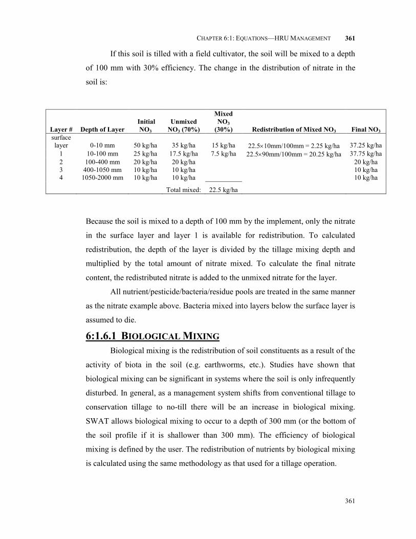
CHAPTER 6:1: EQUATIONS—HRU MANAGEMENT
361
361
If this soil is tilled with a field cultivator, the soil will be mixed to a depth
of 100 mm with 30% efficiency. The change in the distribution of nitrate in the
soil is:
Layer #
Depth of Layer
Initial
NO3
Unmixed
NO3 (70%)
Mixed NO3
(30%)
Redistribution of Mixed NO3
Final NO3 surface layer
0-10 mm
50 kg/ha
35 kg/ha
15 kg/ha
22.510mm/100mm = 2.25 kg/ha
37.25 kg/ha
1 10-100 mm 25 kg/ha 17.5 kg/ha 7.5 kg/ha 22.590mm/100mm = 20.25 kg/ha 37.75 kg/ha 2 100-400 mm 20 kg/ha 20 kg/ha 20 kg/ha 3 400-1050 mm 10 kg/ha 10 kg/ha 10 kg/ha 4 1050-2000 mm 10 kg/ha 10 kg/ha 10 kg/ha Total mixed: 22.5 kg/ha
Because the soil is mixed to a depth of 100 mm by the implement, only the nitrate
in the surface layer and layer 1 is available for redistribution. To calculated
redistribution, the depth of the layer is divided by the tillage mixing depth and
multiplied by the total amount of nitrate mixed. To calculate the final nitrate
content, the redistributed nitrate is added to the unmixed nitrate for the layer.
All nutrient/pesticide/bacteria/residue pools are treated in the same manner
as the nitrate example above. Bacteria mixed into layers below the surface layer is
assumed to die.
6:1.6.1 BIOLOGICAL MIXING Biological mixing is the redistribution of soil constituents as a result of the
activity of biota in the soil (e.g. earthworms, etc.). Studies have shown that
biological mixing can be significant in systems where the soil is only infrequently
disturbed. In general, as a management system shifts from conventional tillage to
conservation tillage to no-till there will be an increase in biological mixing.
SWAT allows biological mixing to occur to a depth of 300 mm (or the bottom of
the soil profile if it is shallower than 300 mm). The efficiency of biological
mixing is defined by the user. The redistribution of nutrients by biological mixing
is calculated using the same methodology as that used for a tillage operation.

362 SWAT THEORETICAL DOCUMENTATION, VERSION 2009
362
Table 6:1-6: SWAT input variables that pertain to tillage.
Variable Name
Definition Input File
Variables in tillage operation line: MONTH/DAY or HUSC Timing of planting operation. .mgt MGT_OP Operation code. MGT_OP = 6 for tillage operation .mgt TILLAGE_ID Tillage implement code from till.dat .mgt Optional inputs: CNOP CN2: Moisture condition II curve number .mgt
Variables in first section of .mgt file BIOMIX Biological mixing efficiency .mgt Variable in tillage database:
EFFMIX Mixing efficiency of tillage operation. till.dat DEPTIL Depth of mixing by tillage operation. till.dat
6:1.7 FERTILIZER APPLICATION The fertilizer operation applies fertilizer or manure to the soil.
Information required in the fertilizer operation includes the timing of the
operation (month and day or fraction of plant potential heat units), the type of
fertilizer/manure applied, the amount of fertilizer/manure applied, and the depth
distribution of fertilizer application.
SWAT assumes surface runoff interacts with the top 10 mm of soil.
Nutrients contained in this surface layer are available for transport to the main
channel in surface runoff. The fertilizer operation allows the user to specify the
fraction of fertilizer that is applied to the top 10 mm. The remainder of the
fertilizer is added to the first soil layer defined in the HRU .sol file.
In the fertilizer database, the weight fraction of different types of nutrients
and bacteria are defined for the fertilizer. The amounts of nutrient added to the
different pools in the soil are calculated:
fertfertfertNO3 NHminNfert 41 6:1.7.1
fertfertfertNH4 NHminNfert 4 6:1.7.2
fertfertorgN orgNfertfrsh 5.0, 6:1.7.3
fertfertorgN orgNfertact 5.0, 6:1.7.4
fertfertP minPfertsolution , 6:1.7.5

CHAPTER 6:1: EQUATIONS—HRU MANAGEMENT
363
363
fertfertorgP orgPfertfrsh 5.0, 6:1.7.6
fertfertorgP orgPferthum 5.0, 6:1.7.7
where NO3fert is the amount of nitrate added to the soil in the fertilizer (kg N/ha),
NH4fert is the amount of ammonium added to the soil in the fertilizer (kg N/ha),
orgNfrsh,fert is the amount of nitrogen in the fresh organic pool added to the soil in
the fertilizer (kg N/ha), orgNact,fert is the amount of nitrogen in the active organic
pool added to the soil in the fertilizer (kg N/ha), Psolution,fert is the amount of
phosphorus in the solution pool added to the soil in the fertilizer (kg P/ha),
orgPfrsh,fert is the amount of phosphorus in the fresh organic pool added to the soil
in the fertilizer (kg P/ha), orgPhum,fert is the amount of phosphorus in the humus
organic pool added to the soil in the fertilizer (kg P/ha), fertminN is the fraction of
mineral N in the fertilizer, fertNH4 is the fraction of mineral N in the fertilizer that
is ammonium, fertorgN is the fraction of organic N in the fertilizer, fertminP is the
fraction of mineral P in the fertilizer, fertorgP is the fraction of organic P in the
fertilizer, and fert is the amount of fertilizer applied to the soil (kg/ha).
If manure is applied, the bacteria in the manure may become attached to
plant foliage or be incorporated into the soil surface layer during application. The
amount of bacteria reaching the ground surface and the amount of bacteria
adhering to the plant foliage is calculated as a function of ground cover. The
ground cover provided by plants is:
1.2
2333.1erfc99532.1
LAIgc 6:1.7.8
where gc is the fraction of the ground surface covered by plants, erfc is the
complementary error function, and LAI is the leaf area index.
The complementary error function frequently occurs in solutions to
advective-dispersive equations. Values for erfc() and erf() (erf is the error
function for ), where is the argument of the function, are graphed in Figure
6:1-1. The figure shows that erf() ranges from –1 to +1 while erfc() ranges
from 0 to +2. The complementary error function takes on a value greater than 1
only for negative values of the argument.

364 SWAT THEORETICAL DOCUMENTATION, VERSION 2009
364
Figure 6:1-1: erf() and erfc() plotted versus
Once the fraction of ground covered by plants is known, the amount of
bacteria applied to the foliage is calculated:
10,
fertfertfrgcbact
lpbactactive
follp
6:1.7.9
10,
fertfertfrgcbact
pbactactive
folp
6:1.7.10
and the amount of bacteria applied to the soil surface is
101
,
fertkfertfrgcbact
bactlpbactactive
fertlpsol
6:1.7.11
1011
,
fertkfertfrgcbact
bactlpbactactive
fertlpsorb
6:1.7.12
101
,
fertkfertfrgcbact
bactpbactactive
fertpsol
6:1.7.13
1011
,
fertkfertfrgcbact
bactpbactactive
fertpsorb
6:1.7.14
where bactlp,fol is the amount of less persistent bacteria attached to the foliage (#
cfu/m2), bactp,fol is the amount of persistent bacteria attached to the foliage (#
cfu/m2), bactlpsol,fert is the amount of less persistent bacteria in the solution pool
added to the soil (# cfu/m2), bactlpsorb,fert is the amount of less persistent bacteria in
the sorbed pool added to the soil (# cfu/m2), bactpsol,fert is the amount of persistent
-1
-0.5
0
0.5
1
1.5
2
-3 -2.000001 -1.0000019 -1.74E-06 0.9999984 1.9999975
erf
( )
an
d e
rfc(
)
-3 -2 -1 0 1 2 3 β
erf(β)
erfc(β)

CHAPTER 6:1: EQUATIONS—HRU MANAGEMENT
365
365
bacteria in the solution pool added to the soil (# cfu/m2), bactpsorb,fert is the amount
of persistent bacteria in the sorbed pool added to the soil (# cfu/m2), gc is the
fraction of the ground surface covered by plants, fractive is the fraction of the
manure containing active colony forming units, fertlpbact is the concentration of
less persistent bacteria in the fertilizer (# cfu/g manure), fertpbact is the
concentration of persistent bacteria in the fertilizer (# cfu/g manure), kbact is the
bacterial partition coefficient, and fert is the amount of fertilizer/manure applied
to the soil (kg/ha).
Table 6:1-7: SWAT input variables that pertain to fertilizer application.
Variable Name
Definition Input File
Variables in fertilizer operation line: MONTH/DAY or HUSC Timing of fertilizer operation. .mgt MGT_OP Operation code. MGT_OP = 3 for fertilizer operation .mgt FERT_ID Type of fertilizer/manure applied (code from fert.dat). .mgt FRT_KG fert: Amount of fertilizer/manure applied (kg/ha) .mgt FRT_SURFACE Fraction of fertilizer applied to top 10 mm .mgt
Variables in fertilizer database: FMINN fertminN: Fraction of mineral nitrogen in the fertilizer fert.dat FMINP fertminP: Fraction of mineral P in the fertilizer fert.dat FORGN fertorgN: Fraction of organic N in the fertilizer fert.dat FORGP fertorgP: Fraction of organic P in the fertilizer fert.dat FNH3N fertNH4: Fraction of mineral N in the fertilizer that is
ammonium
fert.dat
BACTPDB fertpbact: Concentration of persistent bacteria in manure (# cfu/g manure)
fert.dat
BACTLPDB fertlpbact: Concentration of less-persistent bacteria in manure (# cfu/g manure)
fert.dat
BACTKDDB kbact: Bacterial partition coefficient fert.dat
Other variables: BACT_SWF fractive: Fraction of manure applied to land areas that has
active colony forming units
.bsn
6:1.8 AUTO-APPLICATION OF FERTILIZER Fertilization in an HRU may be scheduled by the user or automatically
applied by SWAT. When the user selects auto-application of fertilizer in an HRU,
a nitrogen stress threshold must be specified. The nitrogen stress threshold is a
fraction of potential plant growth. Anytime actual plant growth falls below this
threshold fraction due to nitrogen stress, the model will automatically apply
fertilizer to the HRU. The user specifies the type of fertilizer, the fraction of total

366 SWAT THEORETICAL DOCUMENTATION, VERSION 2009
366
fertilizer applied to the soil surface, the maximum amount of fertilizer that can be
applied during the year, the maximum amount of fertilizer that can be applied in
any one application, and the application efficiency.
To determine the amount of fertilizer applied, an estimate of the amount of
nitrogen that will be removed in the yield is needed. For the first year of
simulation, the model has no information about the amount of nitrogen removed
from the soil by the plant. The nitrogen yield estimate is initially assigned a value
using the following equations:
RUEfryld yldNNest ,, 350 if 0.1optHI 6:1.8.1
RUEfryld yldNNest ,, 1000 if 0.1optHI 6:1.8.2
where yldest,N is the nitrogen yield estimate (kg N/ha), frN,yld is the fraction of
nitrogen in the yield, RUE is the radiation-use efficiency of the plant
(kg/ha(MJ/m2)-1 or 10-1 g/MJ), and HIopt is the potential harvest index for the
plant at maturity given ideal growing conditions. The nitrogen yield estimate is
updated at the end of every simulation year using the equation:
1
,,,
sim
NyrsimNprevest
Nestyr
yldyryldyld 6:1.8.3
where yldest,N is the nitrogen yield estimate update for the current year (kg N/ha),
yldest,Nprev is the nitrogen yield estimate from the previous year (kg N/ha), yrsim is
the year of simulation, yldyr,N is the nitrogen yield target for the current year (kg
N/ha). The nitrogen yield target for the current year is calculated at the time of
harvest using the equation:
effNagNyr fertfrbioyld , 6:1.8.4
where yldyr,N is the nitrogen yield target for the current year (kg N/ha), bioag is the
aboveground biomass on the day of harvest (kg ha-1), frN is the fraction of
nitrogen in the plant biomass calculated with equation 5:2.3.1, and ferteff is the
fertilizer application efficiency assigned by the user. The fertilizer application
efficiency allows the user to modify the amount of fertilizer applied as a function
of plant demand. If the user would like to apply additional fertilizer to adjust for
loss in runoff, ferteff will be set to a value greater than 1. If the user would like to
CHAPTER 6:1: EQUATIONS—HRU MANAGEMENT
367
367
apply just enough fertilizer to meet the expected demand, ferteff will be set to 1. If
the user would like to apply only a fraction of the demand, ferteff will be set to a
value less than 1.
The optimal amount of mineral nitrogen to be applied is calculated:
NNestapp bioNH4NO3yldminN , 6:1.8.5
where minNapp is the amount of mineral nitrogen applied (kg N/ha), yldest,N is the
nitrogen yield estimate (kg N/ha), NO3 is the nitrate content of the soil profile (kg
NO3-N/ha), NH4 is the ammonium content of the soil profile (kg NH4-N/ha), and
bioN is the actual mass of nitrogen stored in plant material (kg N/ha). If the
amount of mineral nitrogen calculated with equation 6:1.8.5 exceeds the
maximum amount allowed for any one application, minNapp is reset to the
maximum value ( mxappapp minNminN , ). The total amount of nitrogen applied
during the year is also compared to the maximum amount allowed for the year.
Once the amount applied reaches the maximum amount allowed for the year
(minNapp,mxyr), SWAT will not apply any additional fertilizer regardless of
nitrogen stress.
Once the amount of mineral nitrogen applied is determined, the total
amount of fertilizer applied is calculated by dividing the mass of mineral nitrogen
applied by the fraction of mineral nitrogen in the fertilizer:
minN
app
fert
minNfert 6:1.8.6
where fert is the amount of fertilizer applied (kg/ha), minNapp is the amount of
mineral nitrogen applied (kg N/ha), and fertminN is the fraction of mineral nitrogen
in the fertilizer.
The type of fertilizer applied in the HRU is specified by the user. In
addition to mineral nitrogen, organic nitrogen and phosphorus and mineral
phosphorus are applied to the HRU. If a manure is applied, bacteria loadings to
the HRU are also determined. The amount of each type of nutrient and bacteria is
calculated from the amount of fertilizer and fraction of the various nutrient types
in the fertilizer as summarized in Section 6:1.7.
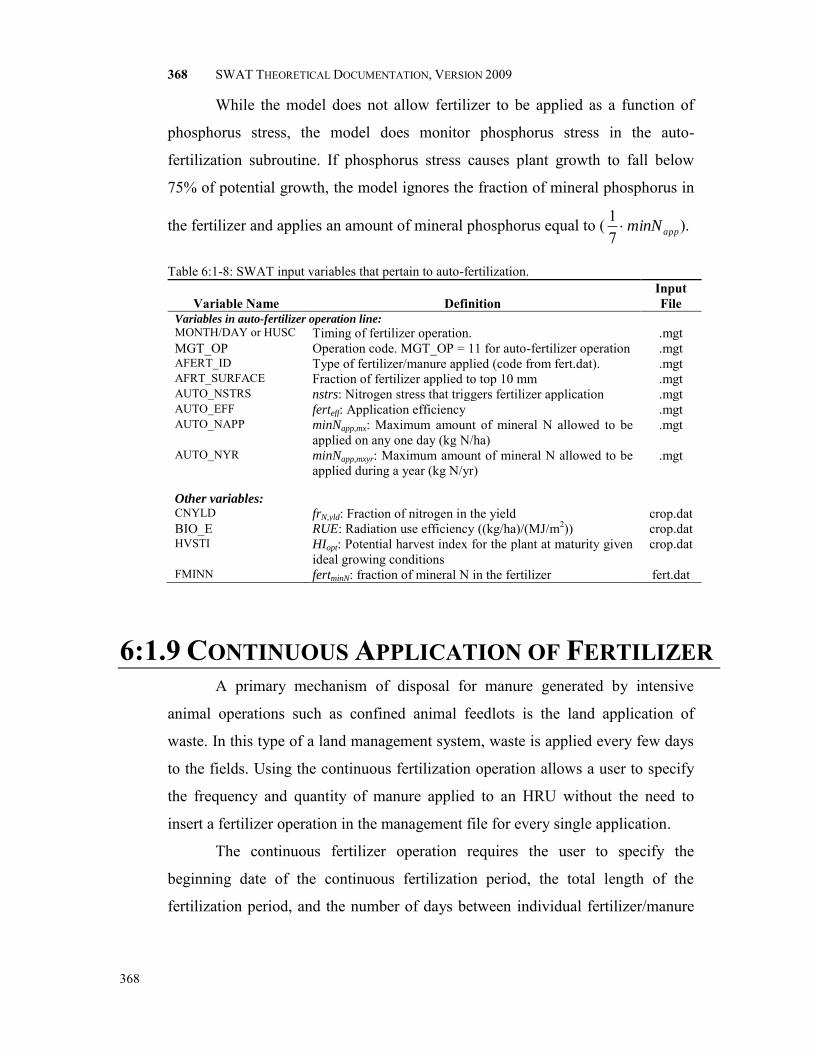
368 SWAT THEORETICAL DOCUMENTATION, VERSION 2009
368
While the model does not allow fertilizer to be applied as a function of
phosphorus stress, the model does monitor phosphorus stress in the auto-
fertilization subroutine. If phosphorus stress causes plant growth to fall below
75% of potential growth, the model ignores the fraction of mineral phosphorus in
the fertilizer and applies an amount of mineral phosphorus equal to ( appminN71 ).
Table 6:1-8: SWAT input variables that pertain to auto-fertilization.
Variable Name
Definition Input File
Variables in auto-fertilizer operation line: MONTH/DAY or HUSC Timing of fertilizer operation. .mgt MGT_OP Operation code. MGT_OP = 11 for auto-fertilizer operation .mgt AFERT_ID Type of fertilizer/manure applied (code from fert.dat). .mgt AFRT_SURFACE Fraction of fertilizer applied to top 10 mm .mgt AUTO_NSTRS nstrs: Nitrogen stress that triggers fertilizer application .mgt AUTO_EFF ferteff: Application efficiency .mgt AUTO_NAPP minNapp,mx: Maximum amount of mineral N allowed to be
applied on any one day (kg N/ha) .mgt
AUTO_NYR minNapp,mxyr: Maximum amount of mineral N allowed to be applied during a year (kg N/yr)
.mgt
Other variables: CNYLD frN,yld: Fraction of nitrogen in the yield crop.dat BIO_E RUE: Radiation use efficiency ((kg/ha)/(MJ/m2)) crop.dat HVSTI HIopt: Potential harvest index for the plant at maturity given
ideal growing conditions
crop.dat
FMINN fertminN: fraction of mineral N in the fertilizer fert.dat
6:1.9 CONTINUOUS APPLICATION OF FERTILIZER
A primary mechanism of disposal for manure generated by intensive
animal operations such as confined animal feedlots is the land application of
waste. In this type of a land management system, waste is applied every few days
to the fields. Using the continuous fertilization operation allows a user to specify
the frequency and quantity of manure applied to an HRU without the need to
insert a fertilizer operation in the management file for every single application.
The continuous fertilizer operation requires the user to specify the
beginning date of the continuous fertilization period, the total length of the
fertilization period, and the number of days between individual fertilizer/manure

CHAPTER 6:1: EQUATIONS—HRU MANAGEMENT
369
369
applications. The amount of fertilizer/manure applied in each application is
specified as well as the type of fertilizer/manure.
Nutrients and bacteria in the fertilizer/manure are applied to the soil
surface. Unlike the fertilization operation or auto-fertilization operation, the
continuous fertilization operation does not allow the nutrient and bacteria loadings
to be partitioned between the surface 10 mm and the part of the 1st soil layer
underlying the top 10 mm. Everything is added to the top 10 mm, making it
available for transport by surface runoff.
Nutrient and bacteria loadings to the HRU are calculated using the
equations reviewed in Section 6:1.7.
Table 6:1-9: SWAT input variables that pertain to continuous fertilization.
Variable Name
Definition Input File
Variables in auto-fertilizer operation line: MONTH/DAY or HUSC Timing of fertilizer operation. .mgt MGT_OP Operation code. MGT_OP = 14 for continuous fertilizer
operation .mgt
CFERT_ID Type of fertilizer/manure applied (code from fert.dat). .mgt FERT_DAYS Duration or length of time (days) the continuous fertilizer
operation takes place .mgt
IFRT_FREQ Application frequeny. Number of days between fertilizer applications
.mgt
CFRT_KG fert: Amount of fertilizer/manure applied (kg/ha) .mgt
6:1.10 PESTICIDE APPLICATION The pesticide operation applies pesticide to the HRU.
Information required in the pesticide operation includes the timing of the
operation (month and day or fraction of plant potential heat units), the type of
pesticide applied, and the amount of pesticide applied.
Field studies have shown that even on days with little or no wind, a
portion of pesticide applied to the field is lost. The fraction of pesticide that
reaches the foliage or soil surface is defined by the pesticide’s application
efficiency. The amount of pesticide that reaches the foliage or ground is:
pestaptpes ef 6:1.10.1
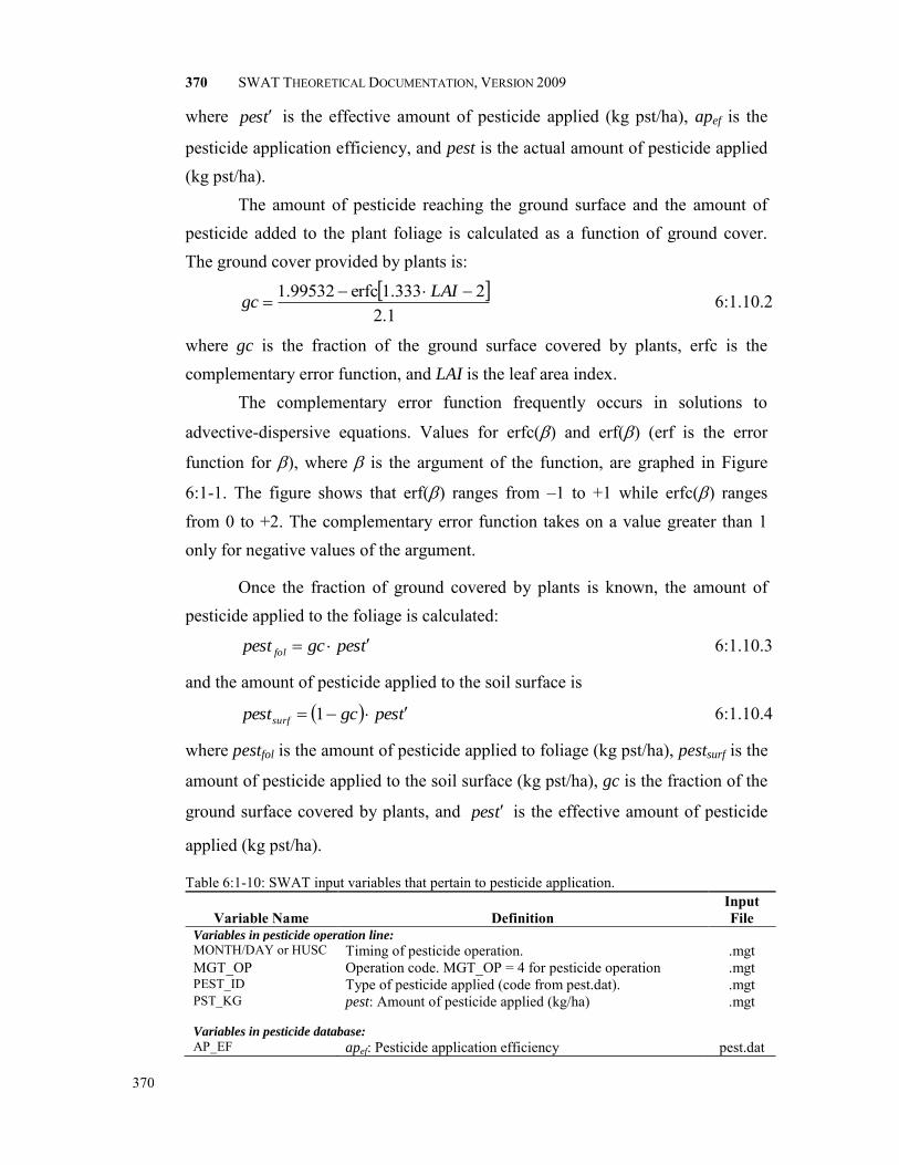
370 SWAT THEORETICAL DOCUMENTATION, VERSION 2009
370
where tpes is the effective amount of pesticide applied (kg pst/ha), apef is the
pesticide application efficiency, and pest is the actual amount of pesticide applied (kg pst/ha). The amount of pesticide reaching the ground surface and the amount of pesticide added to the plant foliage is calculated as a function of ground cover. The ground cover provided by plants is:
1.2
2333.1erfc99532.1
LAIgc 6:1.10.2
where gc is the fraction of the ground surface covered by plants, erfc is the complementary error function, and LAI is the leaf area index.
The complementary error function frequently occurs in solutions to
advective-dispersive equations. Values for erfc() and erf() (erf is the error
function for ), where is the argument of the function, are graphed in Figure
6:1-1. The figure shows that erf() ranges from –1 to +1 while erfc() ranges from 0 to +2. The complementary error function takes on a value greater than 1 only for negative values of the argument.
Once the fraction of ground covered by plants is known, the amount of pesticide applied to the foliage is calculated:
tpesgcpest fol 6:1.10.3
and the amount of pesticide applied to the soil surface is
tpesgcpestsurf 1 6:1.10.4
where pestfol is the amount of pesticide applied to foliage (kg pst/ha), pestsurf is the
amount of pesticide applied to the soil surface (kg pst/ha), gc is the fraction of the
ground surface covered by plants, and tpes is the effective amount of pesticide
applied (kg pst/ha).
Table 6:1-10: SWAT input variables that pertain to pesticide application.
Variable Name
Definition Input File
Variables in pesticide operation line: MONTH/DAY or HUSC Timing of pesticide operation. .mgt MGT_OP Operation code. MGT_OP = 4 for pesticide operation .mgt PEST_ID Type of pesticide applied (code from pest.dat). .mgt PST_KG pest: Amount of pesticide applied (kg/ha) .mgt
Variables in pesticide database: AP_EF apef: Pesticide application efficiency pest.dat

CHAPTER 6:1: EQUATIONS—HRU MANAGEMENT
371
371
6:1.11 NOMENCLATURE CN2 Moisture condition II curve number HIopt Potential harvest index for the plant at maturity given ideal growing conditions
HItrg Target harvest index
LAI Leaf area index of the canopy
NH4 Ammonium content of the soil profile (kg NH4-N/ha) NH4fert Amount of ammonium added to the soil in the fertilizer (kg N/ha) NO3 Nitrate content of the soil profile (kg NO3-N/ha) NO3fert Amount of nitrate added to the soil in the fertilizer (kg N/ha) Psolution,fert Amount of phosphorus in the solution pool added to the soil in the fertilizer
(kg P/ha) PHU Potential heat units or total heat units required for plant maturity where base
temperature is dependant on the plant species (heat units) RUE Radiation-use efficiency of the plant (kg/ha(MJ/m2)-1 or 10-1 g/MJ) apef Pesticide application efficiency bactlpsol,fert Amount of less persistent bacteria in the solution pool added to the soil in the
fertilizer (# cfu/m2) bactlp,fol Amount of less persistent bacteria attached to the foliage (# cfu/m2), bactlpsorb,fert Amount of less persistent bacteria in the sorbed pool added to the soil in
fertilizer (# cfu/m2) bactpsol,fert Amount of persistent bacteria in the solution pool added to the soil in the
fertilizer (# cfu/m2) bactp,fol Amount of persistent bacteria attached to the foliage (# cfu/m2) bactpsorb,fert Amount of persistent bacteria in the sorbed pool added to the soil in fertilizer
(# cfu/m2) bio Total plant biomass on a given day (kg/ha) bioag Aboveground biomass on the day of harvest (kg ha-1) bioN Actual mass of nitrogen stored in plant material (kg N/ha) biotrg Target biomass specified by the user (kg/ha) fert Amount of fertilizer applied (kg/ha) ferteff Fertilizer application efficiency assigned by the user fertlpbact Concentration of less persistent bacteria in the fertilizer (# cfu/g manure) fertminN Fraction of mineral nitrogen in the fertilizer fertminP Fraction of mineral P in the fertilizer fertNH4 Fraction of mineral N in the fertilizer that is ammonium fertorgN Fraction of organic N in the fertilizer fertorgP Fraction of organic P in the fertilizer fertpbact Concentration of persistent bacteria in the fertilizer (# cfu/g manure) fractive Fraction of the manure containing active colony forming units
frN Optimal fraction of nitrogen in the plant biomass for current growth stage frN,yld Fraction of nitrogen in the yield gc Fraction of the ground surface covered by plants harveff Efficiency of the harvest operation

372 SWAT THEORETICAL DOCUMENTATION, VERSION 2009
372
kbact Bacterial partition coefficient minNapp Amount of mineral nitrogen applied (kg N/ha) minNapp,mx Maximum amount of mineral N allowed to be applied on any one day (kg
N/ha) minNapp,mxyr Maximum amount of mineral N allowed to be applied during a year (kg
N/ha) nstrs Nitrogen stress for a given day
orgNact,fert Amount of nitrogen in the active organic pool added to the soil in the fertilizer (kg N/ha)
orgNfrsh,fert Amount of nitrogen in the fresh organic pool added to the soil in the fertilizer (kg N/ha)
orgPfrsh,fert Amount of phosphorus in the fresh organic pool added to the soil in the fertilizer (kg P/ha)
orgPhum,fert Amount of phosphorus in the humus organic pool added to the soil in the fertilizer (kg P/ha)
pest Actual amount of pesticide applied (kg pst/ha) tpes Effective amount of pesticide applied (kg pst/ha)
pestfol Amount of pesticide applied to foliage (kg pst/ha) pestsurf Amount of pesticide applied to the soil surface (kg pst/ha) trapef Fraction of the constituent loading trapped by the filter strip
trapef,bact Fraction of the bacteria loading trapped by the filter strip trapef,sub Fraction of the subsurface flow constituent loading trapped by the filter strip
widthfiltstrip Width of filter strip (m) yldest,N Nitrogen yield estimate (kg N/ha) yldest,Nprev Nitrogen yield estimate from the previous year (kg N/ha) yldyr,N Nitrogen yield target for the current year (kg N/ha) yrsim Year of simulation
6:1.12 REFERENCES Moore, J.A., J.D. Smyth, E.S. Baker, and J.R. Miner. 1988. Evaluating coliform
concentrations in runoff from various animal waste management systems. Special
Report 817: Agricultural Experiment Stations, Oregon State University, Corvallis.

CHAPTER 6:1: EQUATIONS—HRU MANAGEMENT
373
373

374
SECTION 6 CHAPTER 2
EQUATIONS:
WATER MANAGEMENT
Accurately reproducing water management practices can be one of the
most complicated portions of data input for the model. Because water
management affects the hydrologic balance, it is critical that the model is able to
accommodate a variety of management practices. Water management options
modeled by SWAT include irrigation, tile drainage, impounded/depressional
areas, water transfer, consumptive water use, and loadings from point sources.

CHAPTER 6:2: EQUATIONS—WATER MANAGEMENT
375
375
6:2.1 IRRIGATION
Irrigation in an HRU may be scheduled by the user or automatically
applied by SWAT in response to a water deficit in the soil. In addition to
specifying the timing and application amount, the user must specify the source of
irrigation water.
Water applied to an HRU is obtained from one of five types of water
sources: a reach, a reservoir, a shallow aquifer, a deep aquifer, or a source outside
the watershed. In addition to the type of water source, the model must know the
location of the water source (unless the source is outside the watershed). For the
reach, shallow aquifer or deep aquifer, SWAT needs to know the reach number or
subbasin number, respectively, in which the source is located. If a reservoir is
used to supply water, SWAT must know the reservoir number.
If the source of the irrigation water is a reach, SWAT allows additional
input parameters to be set. These parameters are used to prevent flow in the reach
from being reduced to zero as a result of irrigation water removal. Users may
define a minimum in-stream flow, a maximum irrigation water removal amount
that cannot be exceeded on any given day, and/or a fraction of total flow in the
reach that is available for removal on a given day.
For a given irrigation event, SWAT determines the amount of water
available in the source. The amount of water available is compared to the amount
of water specified in the irrigation operation. If the amount available is less than
the amount specified, SWAT will only apply the available water.
6:2.1.1 MANUAL APPLICATION OF IRRIGATION A manual irrigation application can be scheduled by date or by heat units.
Irrigation amount (mm), input by the user, is the amount of water applied that reaches
the soil. An irrigation efficiency factor is applied to account for losses from the
source to the soil including conveyance loss and evaporative loss. The surface runoff
ratio is the fraction of water applied that leaves the field as surface runoff. The
remainder infiltrates into the soil and is subject to the soil water routing algorithms

376 SWAT THEORETICAL DOCUMENTATION, VERSION 2009
376
described in Section 2, Chapter 3. This allows for more realistic simulation of the
soil water profile and application of excess irrigation for leaching salts.
6:2.1.2 AUTO-APPLICATION OF IRRIGATION When the user selects auto-application of irrigation, the application can be
triggered by a water stress threshold or a soil water deficit threshold. The water
stress threshold is a fraction of potential plant growth. Any day actual plant stress
falls below this threshold fraction due to water stress, the model will
automatically apply water up to a maximum amount per application as input by
the user. An irrigation application can also be triggered by a soil water deficit
threshold. When total soil water in the profile falls below field capacity by more
than the soil water deficit threshold, an irrigation application occurs. As with a
manual application, a maximum irrigation amount, irrigation efficiency and
surface runoff ratio are applied to each application.
Table 6:2-1: SWAT input variables that pertain to irrigation.
Variable Name
Definition Input File
Variables in irrigation operation line: MONTH/DAY or HUSC Timing of irrigation operation. .mgt MGT_OP Operation code. MGT_OP = 2 for irrigation operation .mgt IRR_AMT IRR_EFM IRR_SQ
Depth of irrigation water applied on HRU (mm) Irrigation efficiency for manual operation (0-1) Irrigation surface runoff ratio for manual operation (0-1)
.mgt
.mgt
.mgt
Variables in first section of .mgt file IRRSC Type of water body from which irrigation water is obtained .mgt IRRNO Source location .mgt FLOWMIN Minimum in-stream flow (m3/s) .mgt DIVMAX Maximum daily irrigation diversion (mm or 104 m3) .mgt FLOWFR Fraction of available flow allowed to be used for irrigation .mgt
Variables in auto-irrigation operation line: MONTH/DAY or HUSC Initialization of auto-irrigation .mgt MGT_OP WSTRS_ID
Operation code. MGT_OP = 10 for auto-irrigation Auto-irrigation trigger (WSTRS_ID = 0 for plant water stress trigger; WSTRS_ID = 1 for soil water deficit trigger
.mgt
.mgt
AUTO_WSTR IRR_EFF IRR_ASQ
Water stress that triggers irrigation Irrigation efficiency for manual operation (0-1) Irrigation surface runoff ratio for manual operation (0-1)
.mgt
.mgt
.mgt

CHAPTER 6:2: EQUATIONS—WATER MANAGEMENT
377
377
6:2.2 TILE DRAINAGE To simulate tile drainage in an HRU, the user must specify the depth from
the soil surface to the drains, the amount of time required to drain the soil to field
capacity, and the amount of lag between the time water enters the tile till it exits
the tile and enters the main channel.
Tile drainage occurs when the perched water table rises above the depth at
which the tile drains are installed. The amount of water entering the drain on a
given day is calculated:
drainwtbl
drainwtbl
wtrt
FCSWh
hhtile
24exp1 if drainwtbl hh 6:2.2.1
where tilewtr is the amount of water removed from the layer on a given day by tile
drainage (mm H2O), hwtbl is the height of the water table above the impervious
zone (mm), hdrain is the height of the tile drain above the impervious zone (mm),
SW is the water content of the profile on a given day (mm H2O), FC is the field
capacity water content of the profile (mm H2O), and tdrain is the time required to
drain the soil to field capacity (hrs).
Water entering tiles is treated like lateral flow. The flow is lagged using
equations reviewed in Chapter 2:3.
Table 6:2-2: SWAT input variables that pertain to tile drainage.
Variable Name
Definition Input File
DDRAIN Depth to subsurface drain (mm). .mgt TDRAIN tdrain: Time to drain soil to field capacity (hrs) .mgt GDRAIN tilelag: Drain tile lag time (hrs) .mgt
6:2.3 IMPOUNDED/DEPRESSIONAL AREAS Impounded/depressional areas are simulated as a water body overlying a
soil profile in an HRU. This type of ponded system is needed to simulate the
growth of rice, cranberries or any other plant that grows in a waterlogged system.
The simulation and management operations pertaining to impounded/depressional
areas are reviewed in Chapter 8:1.

378 SWAT THEORETICAL DOCUMENTATION, VERSION 2009
378
6:2.4 WATER TRANSFER While water is most typically removed from a water body for irrigation
purposes, SWAT also allows water to be transferred from one water body to
another. This is performed with a transfer command in the watershed
configuration file.
The transfer command can be used to move water from any reservoir or
reach in the watershed to any other reservoir or reach in the watershed. The user
must input the type of water source, the location of the source, the type of water
body receiving the transfer, the location of the receiving water body, and the
amount of water transferred.
Three options are provided to specify the amount of water transferred: a
fraction of the volume of water in the source; a volume of water left in the source;
or the volume of water transferred. The transfer is performed every day of the
simulation.
The transfer of water from one water body to another can be accomplished
using other methods. For example, water could be removed from one water body
via consumptive water use and added to another water body using point source
files.
Table 6:2-3: SWAT input variables that pertain to water transfer.
Variable Name
Definition Input File
DEP_TYPE Water source type .fig DEP_NUM Water source location .fig DEST_TYPE Destination type .fig DEST_NUM Destination location .fig TRANS_AMT Amount of water transferred .fig TRANS_CODE Rule code governing water transfer. .fig
6:2.5 CONSUMPTIVE WATER USE Consumptive water use is a management tool that removes water from the
basin. Water removed for consumptive use is considered to be lost from the
system. SWAT allows water to be removed from the shallow aquifer, the deep
CHAPTER 6:2: EQUATIONS—WATER MANAGEMENT
379
379
aquifer, the reach or the pond within any subbasin in the watershed. Water also
may be removed from reservoirs for consumptive use.
Consumptive water use is allowed to vary from month to month. For each
month in the year, an average daily volume of water removed from the source is
specified. For reservoirs, the user may also specify a fraction of the water
removed that is lost during removal. The water lost in the removal process
becomes outflow from the reservoir.
Table 6:2-4: SWAT input variables that pertain to consumptive water use.
Variable Name
Definition Input File
WUPND(1-12) Average daily water removal from pond in subbasin (104 m3) .wus WURCH(1-12) Average daily water removal from reach in subbasin (104 m3) .wus WUSHAL(1-12) Average daily water removal from shallow aquifer in subbasin
(104 m3) .wus
WUDEEP(1-12) Average daily water removal from deep aquifer in subbasin (104 m3)
.wus
WURESN(1-12) Average daily water removal from reservoir (104 m3) .res WURTNF Fraction of water removal lost in transfer and returned as
reservoir outflow. .res
6:2.6 POINT SOURCE LOADINGS SWAT directly simulates the loading of water, sediment and other
constituents off of land areas in the watershed. To simulate the loading of water
and pollutants from sources not associated with a land area (e.g. sewage treatment
plants), SWAT allows point source information to be read in at any point along
the channel network. The point source loadings may be summarized on a daily,
monthly, yearly, or average annual basis.
Files containing the point source loads are created by the user. The loads
are read into the model and routed through the channel network using rechour,
recday, recmon, recyear, or reccnst commands in the watershed configuration file.
SWAT will read in water, sediment, organic N, organic P, nitrate, soluble P,
ammonium, nitrite, metal, and bacteria data from the point source files. Chapter 2
in the SWAT2009 User’s Manual reviews the format of the command lines in the
watershed configuration file while Chapter 31 in the SWAT2009 User’s Manual
reviews the format of the point source files.

380 SWAT THEORETICAL DOCUMENTATION, VERSION 2009
380
6:2.7 NOMENCLATURE SW Water content of the profile on a given day (mm H2O) FC Field capacity water content of the profile (mm H2O) hdrain Height of the tile drain above the impervious zone (mm) hwtbl Height of the water table above the impervious zone (mm) tdrain Time required to drain the soil to field capacity (hrs) tilewtr Amount of water removed from the layer on a given day by tile drainage (mm
H2O)

CHAPTER 6:2: EQUATIONS—WATER MANAGEMENT
381
381
382
SECTION 6 CHAPTER 3
EQUATIONS:
URBAN AREAS
Most large watersheds and river basins contain areas of urban land use.
Estimates of the quantity and quality of runoff in urban areas are required for
comprehensive management analysis. SWAT calculates runoff from urban areas
with the SCS curve number method or the Green & Ampt equation. Loadings of
sediment and nutrients are determined using one of two options. The first is a set
of linear regression equations developed by the USGS (Driver and Tasker, 1988)
for estimating storm runoff volumes and constituent loads. The other option is to
simulate the buildup and washoff mechanisms, similar to SWMM - Storm Water
Management Model (Huber and Dickinson, 1988).

CHAPTER 6:3: EQUATIONS—URBAN AREAS
383
383
6:3.1 CHARACTERISTICS OF URBAN AREAS
Urban areas differ from rural areas in the fraction of total area that is
impervious. Construction of buildings, parking lots and paved roads increases the
impervious cover in a watershed and reduces infiltration. With development, the
spatial flow pattern of water is altered and the hydraulic efficiency of flow is
increased through artificial channels, curbing, and storm drainage and collection
systems. The net effect of these changes is an increase in the volume and velocity
of runoff and larger peak flood discharges.
Impervious areas can be differentiated into two groups: the area that is
hydraulically connected to the drainage system and the area that is not directly
connected. As an example, assume there is a house surrounded by a yard where
runoff from the roof flows into the yard and is able to infiltrate into the soil. The
rooftop is impervious but it is not hydraulically connected to the drainage system.
In contrast, a parking lot whose runoff enters a storm water drain is hydraulically
connected. Table 6:3-1 lists typical values for impervious and directly connected
impervious fractions in different urban land types.
Table 6:3-1: Range and average impervious fractions for different urban land types. Urban Land Type
Average total impervious
Range total impervious
Average directly connected
impervious
Range directly connected
impervious Residential-High Density
(> 8 unit/acre or unit/2.5 ha)
.60
.44 - .82
.44
.32 - .60 Residential-Medium Density
(1-4 unit/acre or unit/2.5 ha)
.38
.23 - .46
.30
.18 - .36 Residential-Med/Low Density
(> 0.5-1 unit/acre or unit/2.5 ha)
.20
.14 - .26
.17
.12 - .22 Residential-Low Density
(< 0.5 unit/acre or unit/2.5 ha)
.12
.07 - .18
.10
.06 - .14 Commercial .67 .48 - .99 .62 .44 - .92 Industrial .84 .63 - .99 .79 .59 - .93 Transportation .98 .88 - 1.00 .95 .85 – 1.00 Institutional .51 .33 - .84 .47 .30 - .77
During dry periods, dust, dirt and other pollutants build up on the
impervious areas. When precipitation events occur and runoff from the
impervious areas is generated, the runoff will carry the pollutants as it moves
through the drainage system and enters the channel network of the watershed.

384 SWAT THEORETICAL DOCUMENTATION, VERSION 2009
384
6:3.2 SURFACE RUNOFF FROM URBAN AREAS
In urban areas, surface runoff is calculated separately for the directly connected impervious area and the disconnected impervious/pervious area. For directly connected impervious areas, a curve number of 98 is always used. For disconnected impervious/pervious areas, a composite curve number is calculated and used in the surface runoff calculations. The equations used to calculate the composite curve number for disconnected impervious/pervious areas are (Soil Conservation Service Engineering Division, 1986):
tot
dcon
pimptotpcimp
impCNCNimpCNCN
21 if 30.0totimp 6:3.2.1
pimptotpc CNCNimpCNCN if 30.0totimp 6:3.2.2
where CNc is the composite moisture condition II curve number, CNp is the
pervious moisture condition II curve number, CNimp is the impervious moisture
condition II curve number, imptot is the fraction of the HRU area that is
impervious (both directly connected and disconnected), and impdcon is the fraction
of the HRU area that is impervious but not hydraulically connected to the
drainage system.
The fraction of the HRU area that is impervious but not hydraulically
connected to the drainage system, impdcon, is calculated
contotdcon impimpimp 6:3.2.3
where imptot is the fraction of the HRU area that is impervious (both directly
connected and disconnected), and impcon is the fraction of the HRU area that is
impervious and hydraulically connected to the drainage system.
Table 6:3-2: SWAT input variables that pertain to surface runoff calculations in urban areas.
Variable Name
Definition Input File
CN2 CNp: SCS moisture condition II curve number for pervious areas .mgt CNOP CNp: SCS moisture condition II curve number for pervious areas
specified in plant, harvest/kill and tillage operation .mgt
URBCN2 CNimp: SCS moisture condition II curve number for impervious areas
urban.dat
FIMP imptot: fraction of urban land type area that is impervious urban.dat FCIMP impcon: fraction of urban land type area that is connected
impervious urban.dat

CHAPTER 6:3: EQUATIONS—URBAN AREAS
385
385
6:3.3 USGS REGRESSION EQUATIONS
The linear regression models incorporated into SWAT are those described
by Driver and Tasker (1988). The regression models were developed from a
national urban water quality database that related storm runoff loads to urban
physical, land use, and climatic characteristics. USGS developed these equations
to predict loadings in ungaged urban watersheds.
The regression models calculate loadings as a function of total storm
rainfall, drainage area and impervious area. The general equation is
205.2110059.24.25 40
321
tottotday impimpDAR
Y 6:3.3.1
where Y is the total constituent load (kg), Rday is precipitation on a given day (mm
H2O), DA is the HRU drainage area (km2), imptot is the fraction of the total area
that is impervious, and the variables are regression coefficients. The regression
equations were developed in English units, so conversion factors were
incorporated to adapt the equations to metric units: 25.4 mm/inch, 2.59 km2/mi2,
and 2.205 lb/kg.
USGS derived three different sets of regression coefficients that are based
on annual precipitation. Category I coefficients are used in watersheds with less
than 508 mm of annual precipitation. Category II coefficients are used in
watersheds with annual precipitation between 508 and 1016 mm. Category III
coefficients are used in watersheds with annual precipitation greater than 1016
mm. SWAT determines the annual precipitation category for each subbasin by
summing the monthly precipitation totals provided in the weather generator input
file.
Regression coefficients were derived to estimate suspended solid load,
total nitrogen load, total phosphorus load and carbonaceous oxygen demand
(COD). SWAT calculates suspended solid, total nitrogen, and total phosphorus
loadings (the carbonaceous oxygen demand is not currently calculated).
Regression coefficients for these constituents are listed in Table 6:3-3.

386 SWAT THEORETICAL DOCUMENTATION, VERSION 2009
386
Once total nitrogen and phosphorus loads are calculated, they are
partitioned into organic and mineral forms using the following relationships from
Northern Virginia Planning District Commission (1979). Total nitrogen loads
consist of 70 percent organic nitrogen and 30 percent mineral (nitrate). Total
phosphorus loads are divided into 75 percent organic phosphorus and 25 percent
orthophosphate.
Table 6:3-3: Urban regression coefficients (from Driver and Tasker, 1988). Loading
Precipitation Category
0
1
2
3
4 suspended solids I 1778.0 0.867 0.728 0.157 2.367 II 812.0 1.236 0.436 0.202 1.938 III 97.7 1.002 1.009 0.837 2.818 total nitrogen I 20.20 0.825 1.070 0.479 1.258 II 4.04 0.936 0.937 0.692 1.373 III 1.66 0.703 0.465 0.521 1.845 total phosphorus I 1.725 0.884 0.826 0.467 2.130 II 0.697 1.008 0.628 0.469 1.790 III 1.618 0.954 0.789 0.289 2.247 COD I 407.0 0.626 0.710 0.379 1.518 II 151.0 0.823 0.726 0.564 1.451 III 102.0 0.851 0.601 0.528 1.978
I = annual precipitation < 508 mm II = 508 mm < annual precipitation < 1,016 mm III = annual precipitation > 1,016 mm
Table 6:3-4: SWAT input variables that pertain to urban modeling with regression equations.
Variable Name
Definition Input File
IURBAN Urban simulation code .mgt URBLU Urban land type identification number from urban database .mgt FIMP Fraction of HRU that is impervious. imptot = FIMP 100 urban.dat PRECIPITATION Rday: Precipitation on a given day (mm H2O) .pcp HRU_FR Fraction of subbasin area in HRU .hru SUB_KM Area of subbasin (km2) .sub PCPMM(mon) Average amount of precipitation falling in month (mm H2O) .wgn
6:3.4 BUILD UP/WASH OFF In an impervious area, dust, dirt and other constituents are built up on
street surfaces in periods of dry weather preceding a storm. Build up may be a
function of time, traffic flow, dry fallout and street sweeping. During a storm
runoff event, the material is then washed off into the drainage system. Although

CHAPTER 6:3: EQUATIONS—URBAN AREAS
387
387
the build up/wash off option is conceptually appealing, the reliability and
credibility of the simulation may be difficult to establish without local data for
calibration and validation (Huber and Dickinson, 1988).
When the build up/wash off option is used in SWAT, the urban hydrologic
response unit (HRU) is divided into pervious and impervious areas. Management
operations other than sweep operations are performed in the pervious portion of
the HRU. Sweep operations impact build up of solids in the impervious portion of
the HRU. For the pervious portion of the HRU, sediment and nutrient loadings are
calculated using the methodology summarized in Chapters 4:1 and 4:2. The
impervious portion of the HRU uses the build up/wash off algorithm to determine
sediment and nutrient loadings.
The build up/wash off algorithm calculates the build up and wash off of
solids. The solids are assumed to possess a constant concentration of organic and
mineral nitrogen and phosphorus where the concentrations are a function of the
urban land type.
Build up of solids is simulated on dry days with a Michaelis-Menton
equation:
tdt
tdSEDSED
half
mx
6:3.4.1
where SED is the solid build up (kg/curb km) td days after the last occurrence of
SED = 0 kg/curb km, SEDmx is the maximum accumulation of solids possible for
the urban land type (kg/curb km), and thalf is the length of time needed for solid
build up to increase from 0 kg/curb km to ½ SEDmx (days). A dry day is defined
as a day with surface runoff less than 0.1 mm. An example build-up curve is
shown in Figure 6:3-1. As can be seen from the plot, the Michaelis-Menton
function will initially rise steeply and then approach the asymptote slowly.

388 SWAT THEORETICAL DOCUMENTATION, VERSION 2009
388
Figure 6:3-1: Build-up function for solids in urban areas.
The two parameters that determine the shape of this curve are SEDmx and
thalf. These parameters are a function of the urban land type.
Wash off is the process of erosion or solution of constituents from an
impervious surface during a runoff event. An exponential relationship is used to
simulate the wash off process (Huber and Dickinson, 1988):
tkk
sed eSEDY 10 6:3.4.2 where Ysed is the cumulative amount of solids washed off at time t (kg/curb km),
SED0 is the amount of solids built up on the impervious area at the beginning of
the precipitation event (kg/curb km), and kk is a coefficient.
The coefficient, kk, may be estimated by assuming it is proportional to the
peak runoff rate:
peakcoef qurbkk 6:3.4.3
where urbcoef is the wash off coefficient (mm-1) and qpeak is the peak runoff rate
(mm/hr).
The original default value for urbcoef was calculated as 0.18 mm-1 by
assuming that 13 mm of total runoff in one hour would wash off 90% of the initial
surface load. Later estimates of urbcoef gave values ranging from 0.002-0.26 mm-1.
Huber and Dickinson (1988) noted that values between 0.039 and 0.390 mm-1 for
urbcoef give sediment concentrations in the range of most observed values. They
also recommended using this variable to calibrate the model to observed data.
0
10
20
30
40
50
60
70
80
90
100

CHAPTER 6:3: EQUATIONS—URBAN AREAS
389
389
To convert the sediment loading from units of kg/curb km to kg/ha, the
amount of sediment removed by wash off is multiplied by the curb length density.
The curb length density is a function of the urban land type. Nitrogen and
phosphorus loadings from the impervious portion of the urban land area are
calculated by multiplying the concentration of nutrient by the sediment loading.
6:3.4.1 STREET CLEANING Street cleaning is performed in urban areas to control buildup of solids and
trash. While it has long been thought that street cleaning has a beneficial effect on
the quality of urban runoff, studies by EPA have found that street sweeping has
little impact on runoff quality unless it is performed every day (U.S.
Environmental Protection Agency, 1983).
SWAT performs street sweeping operations only when the build up/wash
off algorithm is specified for urban loading calculations. Street sweeping is
performed only on dry days, where a dry day is defined as a day with less than 0.1
mm of surface runoff. The sweeping removal equation (Huber and Dickinson,
1988) is:
refffrSEDSED av 10 6:3.4.4
where SED is amount of solids remaining after sweeping (kg/curb km), SED0 is
the amount of solids present prior to sweeping (kg/curb km), frav is the fraction of
the curb length available for sweeping (the availability factor), and reff is the
removal efficiency of the sweeping equipment. The availability factor and
removal efficiency are specified by the user.

390 SWAT THEORETICAL DOCUMENTATION, VERSION 2009
390
Table 6:3-5: Removal efficiencies (fraction removed) from street cleaner path (from Pitt, 1979) Street Cleaning Program and Street Surface Loading Conditions
Total Solids
BOD5 COD KN PO4 Pesticides
Vacuum Street Cleaner (5.5-55 kg/curb km)
1 pass .31 .24 .16 .26 .08 .33 2 passes .45 .35 .22 .37 .12 .50 3 passes .53 .41 .27 .45 .14 .59
Vacuum Street Cleaner (55-280 kg/curb km)
1 pass .37 .29 .21 .31 .12 .40 2 passes .51 .42 .29 .46 .17 .59 3 passes .58 .47 .35 .51 .20 .67
Vacuum Street Cleaner (280-2820 kg/curb km)
1 pass .48 .38 .33 .43 .20 .57 2 passes .60 .50 .42 .54 .25 .72 3 passes .63 .52 .44 .57 .26 .75
Mechanical Street Cleaner (50-500 kg/curb km)
1 pass .54 .40 .31 .40 .20 .40 2 passes .75 .58 .48 .58 .35 .60 3 passes .85 .69 .59 .69 .46 .72
Flusher .30 a a a a a Mechanical Street Cleaner followed
by a Flusher
.80
b
b
b
b
b
a: efficiency fraction estimated .15 to .40 b: efficiency fraction estimated .35 to 1.00 The availability factor, frav, is the fraction of the curb length that is
sweepable. The entire curb length is often not available for sweeping due to the
presence of cars and other obstacles.
The removal efficiency of street sweeping is a function of the type of
sweeper, whether flushing is a part of the street cleaning process, the quantity of
total solids, the frequency of rainfall events and the constituents considered.
Removal efficiency can vary depending on the constituent being considered, with
efficiencies being greater for particulate constituents. The removal efficiencies for
nitrogen and phosphorus are typically less than the solid removal efficiency (Pitt,
1979). Because SWAT assumes a set concentration of nutrient constituents in the
solids, the same removal efficiency is in effect used for all constituents. Table
6:3-5 provides removal efficiencies for various street cleaning programs.

CHAPTER 6:3: EQUATIONS—URBAN AREAS
391
391
Table 6:3-6: SWAT input variables that pertain to build up/wash off.
Variable Name
Definition Input File
IURBAN Urban simulation code .mgt URBLU Urban land type identification number from urban database .mgt DIRTMX SEDmx: maximum amount of solids allowed to build up on
impervious areas (kg/curb km) urban.dat
THALF thalf: number of days for amount of solids on impervious area to build up from 0 kg/curb km to ½ SEDmx
urban.dat
URBCOEF urbcoef: wash off coefficient (mm-1) urban.dat CURBDEN curb length density in urban land type (km/ha) urban.dat TNCONC concentration of total nitrogen in suspended solid load (mg N/kg) urban.dat TPCONC concentration of total phosphorus in suspended solid load (mg
N/kg) urban.dat
TNO3CONC concentration of nitrate in suspended solid load (mg N/kg) urban.dat SWEEPEFF reff: removal efficiency of the sweeping equipment .mgt FR_CURB frav: fraction of the curb length that is sweepable. .mgt
6:3.5 NOMENCLATURE CN Curve number DA HRU drainage area (km2) Rday Amount of rainfall on a given day (mm H2O) SED Solid build up (kg/curb km) SEDmx Maximum accumulation of solids possible for the urban land type (kg/curb km) Y Total constituent load (kg) Ysed Cumulative amount of solids washed off at time t (kg/curb km)
frav Fraction of the curb length available for sweeping (the availability factor) impcon Fraction of the HRU area that is impervious and hydraulically connected to the
drainage system impdcon Fraction of the HRU area that is impervious but not hydraulically connected to the
drainage system
imptot Fraction of the HRU area that is impervious (both connected and disconnected) kk Coefficient in urban wash off equation
qpeak Peak runoff rate (mm/hr) reff Removal efficiency of the sweeping equipment thalf Length of time needed for solid build up to increase from 0 kg/curb km to ½
SEDmx (days) urbcoef Wash off coefficient (mm-1) 0 Coefficient for USGS regression equations for urban loadings 1 Coefficient for USGS regression equations for urban loadings 2 Coefficient for USGS regression equations for urban loadings 3 Coefficient for USGS regression equations for urban loadings 4 Coefficient for USGS regression equations for urban loadings

392 SWAT THEORETICAL DOCUMENTATION, VERSION 2009
392
6:3.6 REFERENCES
Driver, N.E. and G.D. Tasker. 1988. Techniques for estimation of storm-runoff
loads, volumes, and selected constituent concentrations in urban
watersheds in the United States. U.S. Dept. of the Interior, U.S. Geological
Survey: Books and Open-File Reports Section 88-191.
Huber, W.C. and R.E. Dickinson. 1988. Storm water management model, version
4: user’s manual. U.S. Environmental Protection Agency, Athens, GA.
Northern Virginia Planning District Commission. 1979. Guidebook for screening
urban nonpoint pollution management strategies: a final report prepared
for Metropolitan Washington Council of Governments. Northern Virginia
Planning District Commission, Falls Church, VA.
Pitt, R. 1979. Demonstration of non-point pollution abatement through improved
street cleaning practices. EPA-600/2-79-161 (NTIS PB80-108988), U.S.
Environmental Protection Agency, Cincinnati, OH.
Soil Conservation Service Engineering Division. 1986. Urban hydrology for small
watersheds. U.S. Department of Agriculture, Technical Release 55.
U.S. Environmental Protection Agency. 1983. Results of the nationwide urban
runoff program; Volume 1 final report. NTIS PB84-185552, U.S.
Environmental Protection Agency, Washington, D.C.

CHAPTER 6:3: EQUATIONS—URBAN AREAS
393
393

394
SECTION 6 CHAPTER 4
EQUATIONS:
SEPTIC SYSTEMS
On-site wastewater systems (OWSs) are considered the cause of
significant non-point source pollution to water bodies, especially in rural areas
and suburban areas. Quantifying their effects on water quality is important
(McCray et al., 2005). Among the several conceptual and (or) mathematical
models, a biozone algorithm proposed by Siegrist et al. (2005) was adapted to
current work due to the fact that the algorithm fully describes biozone processes,
validated at watershed scale, and provides coefficients specifically developed for
biozone processes that were calibrated to field scale experimental data. In this
algorithm, septic tank effluent directly drains into subsurface soil layer
(infiltrative surfaces) affecting soil moisture content and the percolation of soil
water through the vadose zone. The amount of percolation is regulated by
unsaturated hydraulic conductivity as a function of soil moisture content. Total
suspended solid (TSS), biochemical oxygen demand (BOD) and nutrients in the
septic tank effluent (STE) trigger complex bio-physical processes in the biozone
which, in turn, affect the hydraulics of soil water. The accumulation of TSS and

CHAPTER 6:4: EQUATIONS—SEPTIC SYSTEMS
395
395
plaque (i.e., dead bodies of biomass) in the pore space causes clogging and
eventually hydraulic failure of the onsite wastewater system. The concentration of
nutrients, BOD, and Fecal Coliform is estimated by a first-order decay equation
based on the reaction coefficients specifically developed for each constituent by
Siegrist et al. (2005). The biozone is considered as a control volume either on top
of soil layer 1 or wedged in between soil layer 1 and soil layer 2 depending on the
soil thickness. This control volume will accept the OWS effluent as well as
infiltration from above. It can output flow vertically below and can contribute to
detention storage on the surface (if the biozone layer is fully saturated).
6:4.1 BIOZONE ALGORITHM
6:4.1.1 BUILDUP OF LIVE BACTERIAL BIOMASS The biozone layer is formed as a biologically active layer in the soil
absorption system near the infiltrative surface by the growth of microorganisms
feeding on the organic matter (BOD) of the septic tank effluent (See Figure 6:4-1).
The amount of live bacteria biomass in the biozone is estimated using a mass
balance equation assuming the biozone as a control volume. The mass balance
equation of microorganisms (live bacteria biomass) in the control volume is then
estimated by:
sloughmortrespBODpinBODSTE RRRCICQdt
Biod , (1)
where Bio is the amount of live bacteria biomass in biozone (kg/ha), CBOD,in is the
BOD concentration in the STE (mg/L), CBOD is the BOD concentration in biozone
(mg/L), is gram of live bacteria growth to gram of BOD in STE (conversion
factor), QSTE is the flow rate of STE (m3/day), Ip is the amount of percolation out
of the biozone (m3/day), Rresp is the amount of respiration of bacteria (kg/ha), R-
mort is the amount of mortality of bacteria (kg/ha), and Rslough is the amount of
sloughed off bacteria (kg/ha).
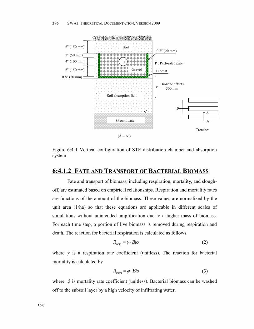
396 SWAT THEORETICAL DOCUMENTATION, VERSION 2009
396
Figure 6:4-1 Vertical configuration of STE distribution chamber and absorption system
6:4.1.2 FATE AND TRANSPORT OF BACTERIAL BIOMASS Fate and transport of biomass, including respiration, mortality, and slough-
off, are estimated based on empirical relationships. Respiration and mortality rates
are functions of the amount of the biomass. These values are normalized by the
unit area (1/ha) so that these equations are applicable in different scales of
simulations without unintended amplification due to a higher mass of biomass.
For each time step, a portion of live biomass is removed during respiration and
death. The reaction for bacterial respiration is calculated as follows.
BioRresp (2)
where is a respiration rate coefficient (unitless). The reaction for bacterial
mortality is calculated by
BioRmort (3)
where is mortality rate coefficient (unitless). Bacterial biomass can be washed
off to the subsoil layer by a high velocity of infiltrating water.
P
6 (150 mm)
2 (50 mm)
4 (100 mm)
6 (150 mm)
0.8 (20 mm)
0.8 (20 mm)
Biomat
Soil
Gravel
Soil absorption field
Groundwater
P : Perforated pipe
Biozone effects 300 mm
A
A’
(A – A’) Trenches

CHAPTER 6:4: EQUATIONS—SEPTIC SYSTEMS
397
397
pslough vR (4)
where vp is the pore velocity in the biozone layer (mm/day), is a linear
coefficient (kg/ha), and is an exponential coefficient (unitless). Equations (2) to
(4) are highly dependent on empirical calibration coefficients and the nature of
these processes makes it difficult to validate the model equations.
A portion of dead body of biomass becomes plaque. Total solids in the
STE may contribute to increasing plaque accumulation in the pore space. Plaque
can be sloughed off from biozone by high pore velocity of infiltrating water. As
the amount of live biomass increases in the biozone, plaque also increases. The
rate of change in plaque is computed by a mass balance equation.
slough
d
STE
mort RA1000
TSQR
dt
plaqued
(5)
where plaque is the amount of dead bacteria biomass and residue (kg/ha), is a
calibration parameter to convert total solids in STE to plaque (unitless), TS is the
total solids contained in STE (mg/l), and Ad is the area of drain field (ha).
6:4.1.3 FIELD CAPACITY Unlike natural soil conditions, the field capacity of a biozone dynamically
changes with time due to the development of filamentous material of live bacterial
biomass allowing the biozone layer to retain additional water. Therefore, temporal
change in the biozone field capacity is related to the amount of biomass in the
layer. This is shown by the equation:
bm
1t
f
1t
s
1t
f
t
f10
dt
Biod
(6)
where f t is field capacity at the end of the day (mm), f
t-1 is field capacity at the
beginning of the day (mm), st-1 is saturated moisture content at the beginning of
the day (mm), bm is the density of live bacterial biomass (~1000 kg/m3 ),

398 SWAT THEORETICAL DOCUMENTATION, VERSION 2009
398
is field capacity coefficient 1 (unitless), and is field capacity coefficient 2
(unitless).
6:4.1.4 CLOGGING EFFECT ON HYDRAULIC
CONDUCTIVITY Soil clogging decreases porosity in the biozone with inert and biological
materials. With the reduced soil porosity, the hydraulic conductivity of soil
decreases with time (USEPA, 1980). A field-scale experiment suggests the
reduction in hydraulic conductivity in the biozone is primarily influenced by STE
loading rate and the type of infiltrative surface (Bumgarner and McCray, 2007).
Weintraub et al. (2002) proposed a relationship between the biozone hydraulic
conductivity and soil moisture contents.
fs
f
satbz KK
(7)
where Kbz is biozone hydraulic conductivity (mm/hr), Ksat is saturated hydraulic
conductivity of soil (mm/hr), and is moisture content of biozone (mm). An
advantage of this model is that, Kb is directly related to Ks and the soil moisture
content. The theoretical basis on the formulation of the equation is not presented
in the literature; instead, the formula is indirectly validated by comparing
percolation to the subsoil layer as a function of time.
6:4.1.5 SOIL MOISTURE AND PERCOLATION Soil porosity (or saturated moisture content) is generally constant in
natural soil; however, the porosity of biozone changes with time. The actual
porosity of biozone decreases as the suspended solids from STE accumulate in the
pore space and the mineralized biomass (dead body) increases in the biozone.
bm
sis
plaque
(8)
where si is initial soil porosity with zero plaque (mm). The moisture content at
each time step is estimated using the mass balance of water within the biozone.
latp
d
STE1tt QETIA10
Q
(9)

CHAPTER 6:4: EQUATIONS—SEPTIC SYSTEMS
399
399
where ET is evaportranspiration from biozone (mm/day) and Qlat is lateral flow
(mm/day). Percolation to a subsoil layer is triggered if moisture content exceeds
the field capacity in the biozone layer. Potential percolation is the maximum
amount of water that can percolate during the time interval.
tKI bzpotp , (10)
where Ip,pot is the potential amount of percolation (mm/day). The amount of water
percolating to the sub-soil layer is calculated using storage routing methodology
(Neitsch et al., 2005).
perc
fexcesspTT
t1I exp)(, fif
0I excessp , fif (11)
where Ip,excess is the minimum amount of percolation (mm/day) and TTperc is travel
time for percolation (TTperc=( s - f)/Kbz) in hour. The actual percolation is the
smaller of the potential and minimum percolation.
),( ,, excessppotpp IIminI (12)
6:4.1.6 NITROGEN, BOD, FECAL COLIFORM Transformation and removal of pollutants in the biozone is directly related
with the population of live bacteria biomass and bio-physical processes in the
biozone layer. The fate of pollutants including Nitrogen, BOD, and Fecal
Coliform is estimated by a first order reaction equation:
tK
ikendkkeCC
,, (13)
where Ck, end is concentration of k constituent in the biozone at the end of the day
(mg/L), Ck, i is concentration of k constituent in the biozone at the beginning of
the day (mg/L), and Kk is a first order reaction rate (1/day), which is a function of
the total biomass of live bacteria and a reaction rate coefficient.
BioV
AKK
bzsi
dk1
k
, (14)
where K1, k is the reaction rate calibration parameter for each constituent k (m3/kg)
and Vbz is the volume of the biozone (m3). The various constituents included are
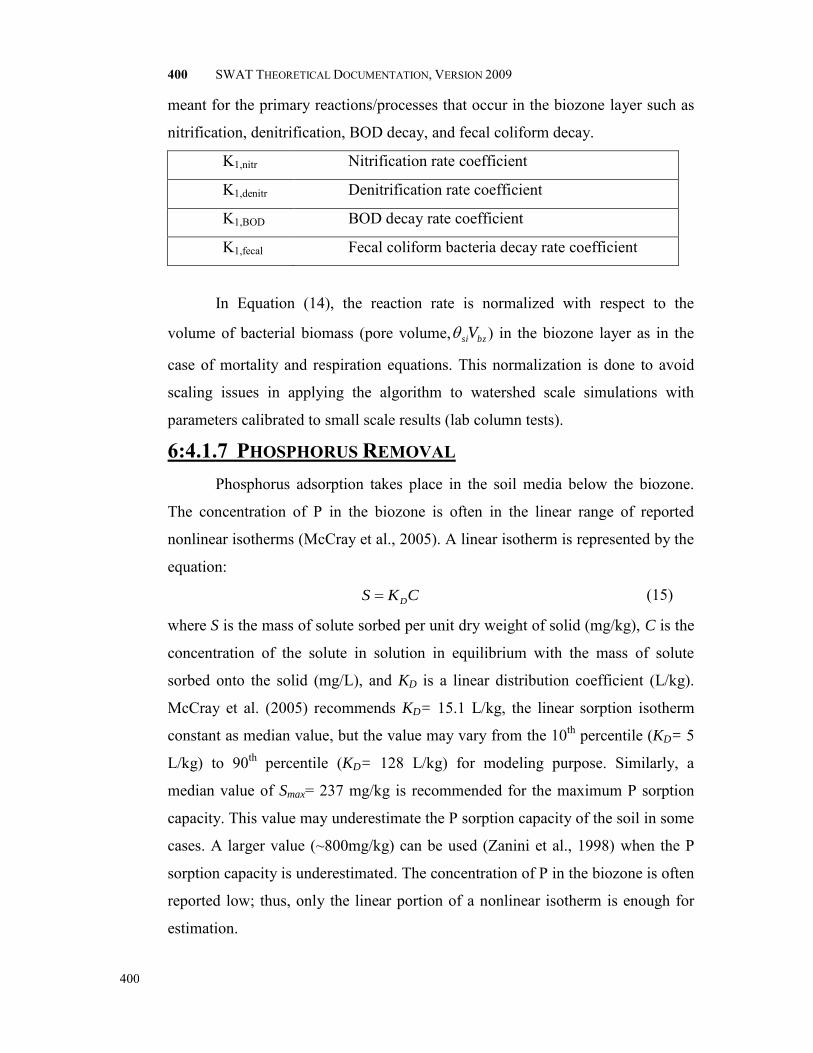
400 SWAT THEORETICAL DOCUMENTATION, VERSION 2009
400
meant for the primary reactions/processes that occur in the biozone layer such as
nitrification, denitrification, BOD decay, and fecal coliform decay.
K1,nitr Nitrification rate coefficient
K1,denitr Denitrification rate coefficient
K1,BOD BOD decay rate coefficient
K1,fecal Fecal coliform bacteria decay rate coefficient
In Equation (14), the reaction rate is normalized with respect to the
volume of bacterial biomass (pore volume, bzsiV ) in the biozone layer as in the
case of mortality and respiration equations. This normalization is done to avoid
scaling issues in applying the algorithm to watershed scale simulations with
parameters calibrated to small scale results (lab column tests).
6:4.1.7 PHOSPHORUS REMOVAL Phosphorus adsorption takes place in the soil media below the biozone.
The concentration of P in the biozone is often in the linear range of reported
nonlinear isotherms (McCray et al., 2005). A linear isotherm is represented by the
equation:
CKS D (15)
where S is the mass of solute sorbed per unit dry weight of solid (mg/kg), C is the
concentration of the solute in solution in equilibrium with the mass of solute
sorbed onto the solid (mg/L), and KD is a linear distribution coefficient (L/kg).
McCray et al. (2005) recommends KD= 15.1 L/kg, the linear sorption isotherm
constant as median value, but the value may vary from the 10th percentile (KD= 5
L/kg) to 90th percentile (KD= 128 L/kg) for modeling purpose. Similarly, a
median value of Smax= 237 mg/kg is recommended for the maximum P sorption
capacity. This value may underestimate the P sorption capacity of the soil in some
cases. A larger value (~800mg/kg) can be used (Zanini et al., 1998) when the P
sorption capacity is underestimated. The concentration of P in the biozone is often
reported low; thus, only the linear portion of a nonlinear isotherm is enough for
estimation.

CHAPTER 6:4: EQUATIONS—SEPTIC SYSTEMS
401
401
Phosphorus sorption isotherm described in Equation (15) gives an estimate
of P sorption capacity given the P concentration and the distribution coefficient.
According to this equation, effluent P concentration leaching to sub-soil layer
should be zero until the soil is saturated withP; however, small amount of soluble
P leaches to sub-soil layer with daily inflow of P to the biozone. The effluent P
concentration is estimated by a linear relationship suggested by Bond et al. (2006)
in which the outflow P concentration is proportional to the total amount P in the
soil layer based on soil type as depicted in Figure 6:4-2.
Figure 6:4-2 Water-soluble P as a function of Mehlich-3 P for native Autryville loamy sand, Wasda muck, Georgeville silt loam, and Pacolet sandy clay loam soils (Bond et al., 2006).
6:4.1.8 MODEL ASSUMPTIONS After STE effluent passes through the biozone, it is discharged into the
soil layers below, where the constituents are subject to additional transport/fate
processes that are expected to occur in natural soils. Siegrist et al. (2005) have

402 SWAT THEORETICAL DOCUMENTATION, VERSION 2009
402
made the following assumptions to represent the physical system of biozone
algorithm development based on laboratory observations and available knowledge.
1. Typical biozone thickness is 2-5 cm.
2. The biozone receives a continuous daily loading of STE.
Intermittent dosing over the course of one day is not considered.
3. Depending on the climatic region, bermuda grass or similar type of
grass is the typical vegetation seen above drainfield.
4. No STE inflow occurs if soil temperature goes below the freezing
point and the biozone processes become inactive.
5. After a hydraulic failure, the model starts counting the failure days
once the STE saturates the upper soil layers completely. Therefore,
the initial several days after the hydraulic failure are not counted as
failing period.
6. A failing system automatically turns to a fresh new active system
after a user specified failing period (typically 2-3 months).
7. Total solids and TDS concentrations of STE are the same.
6:4.2 INTEGRATION OF BIOZONE ALGORITHM
The biozone algorithm was integrated into the latest version of (SWAT
version 2009 and the GIS interface version ArcSWAT 2009). Each unit of onsite
septic systems is represented by a septic HRU. A septic HRU represents either
one OWS or a hypothetical system that aggregates several OWSs that have
similar HRU properties such as soil type, landuse and slope. In the latter case,
septic HRUs in a subbasin are not spatially referenced and only lumped
simulation is available. Septic HRUs are generated during the GIS interface
processing based on the septic land use type defined by the users. Biozone and
other properties of a septic system specific to a HRU is listed in septic input files
(*.sep files). The septic water quality database developed based on literature lists
STE loading rate and pollutants concentration in STE of the conventional system
25 kinds of advanced systems and an untreated effluent system (septwq.dat).
Pollutant characteristics included in the water quality database are per capita

CHAPTER 6:4: EQUATIONS—SEPTIC SYSTEMS
403
403
septic effluent flow rate, Bio-chemical Oxygen Demand (BOD), Total Suspended
Solid (TSS), Total Nitrogen (TN), ammonium, nitrite, nitrate, organic nitrogen,
Total Phosphorus (TP), phosphate, organic P, and Fecal Coliform. A generic type
for conventional system and advanced system are listed as the first and the second
in the water quality database list, so the user can select these types with limited
information. The hydrologic linkage to SWAT allows daily STE directly to be
introduced to the biozone layer by increasing the soil moisture content in the
subroutine percmain. The movement of soil water through percolation in and out
of the biozne layer is then simulated by a SWAT soil water model in percmicro.
The movement of nutrients through soil profile from the biozone layer is
simulated by a combination of nutrient modules in SWAT and biozone. SWAT
septic input parameters are presented in the updated SWAT Input/Output File
Documentation (Neitsch et al., 2010).
6:4.2.1 SIMULATING ACTIVE AND FAILING SYSTEMS In SWAT modeling, active systems are septic systems that are in operation
or functioning as per guidelines and failing systems are septic systems that are
subject to hydraulic failure and the effluent discharged differ from the standards.
A typical service life span of an OWS ranges from 10 to 25 years depending on
maintenance, pollutant loading rate, soil conditions and other factors. A septic
HRU starting as an active system becomes a failing system as the biozone gets
clogged by TSS and plaque of biomass. In the SWAT biozone module, biozone
clogging, or hydraulic failure, is the main cause of system failure. There are other
types of failing, but they are difficult to model in the SWAT structure and thus
hydraulic failure was modeled as the only type of failing.
The schematic of the SWAT biozone algorithm is described in Figure 6:4-
3. The biozone processes in septic HRUs are simulated on a daily basis as a
subbasin-level. The biozone subroutine is called within the HRU iteration loop
whenever the current HRU is septic. Each septic HRU is simulated based on a
maintenance plan in which a failing system is assumed to be fixed and re-
activated in two to three months time. In an active system, saturated water content

404 SWAT THEORETICAL DOCUMENTATION, VERSION 2009
404
gets lower as plaque fills in the soil pore space and field capacity increases as the
amount of live bacteria biomass grows as filamentous biomass soaks up soil
water. System failure occurs when the soil achieves saturated water content and
field capacity. The model starts counting the number of days as the system fails
and remains as a failing system. STE migrates to upper soil layers as water does
not percolate through the bottom of the biozone layer. Depending on the thickness
of soil above the biozone layer, it may take a few days to months until failure
creates STE surface ponding. As STE migrates to upper soil layers, the nutrients
in the STE are transported along with the STE. The amount of nutrients that
transports to the upper soil layers is estimated based on the nutrient concentration
in STE and the amount of water that migrates to the upper layer. There are no
special treatment processes that apply to the nutrients in failing septic systems. If
the number of days a septic system remained as failing exceeds the designed time,
the failing system is updated to an active system and related properties are
reinitialized as a fresh active system. An active system simulates soil water
hydraulics and pollutants decay by executing the biozone equations described
above.

CHAPTER 6:4: EQUATIONS—SEPTIC SYSTEMS
405
405
Figure 6:4-3 Schematic of computations in the biozone algorithm. An active system becomes failing due to clogging in the biozone, then gets repaired to a new active system in several months of time period
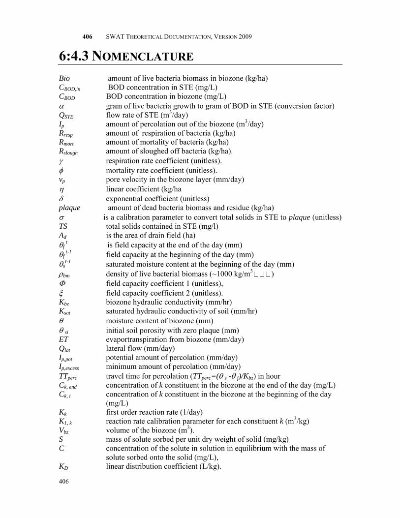
406 SWAT THEORETICAL DOCUMENTATION, VERSION 2009
406
6:4.3 NOMENCLATURE Bio amount of live bacteria biomass in biozone (kg/ha) CBOD,in BOD concentration in STE (mg/L) CBOD BOD concentration in biozone (mg/L) gram of live bacteria growth to gram of BOD in STE (conversion factor) QSTE flow rate of STE (m3/day) Ip amount of percolation out of the biozone (m3/day) Rresp amount of respiration of bacteria (kg/ha) Rmort amount of mortality of bacteria (kg/ha) Rslough amount of sloughed off bacteria (kg/ha). respiration rate coefficient (unitless). mortality rate coefficient (unitless). vp pore velocity in the biozone layer (mm/day) linear coefficient (kg/ha exponential coefficient (unitless) plaque amount of dead bacteria biomass and residue (kg/ha) is a calibration parameter to convert total solids in STE to plaque (unitless) TS total solids contained in STE (mg/l) Ad is the area of drain field (ha) f
t is field capacity at the end of the day (mm) f
t-1 field capacity at the beginning of the day (mm) s
t-1 saturated moisture content at the beginning of the day (mm) bm density of live bacterial biomass (~1000 kg/m3 ) field capacity coefficient 1 (unitless), field capacity coefficient 2 (unitless). Kbz biozone hydraulic conductivity (mm/hr) Ksat saturated hydraulic conductivity of soil (mm/hr) moisture content of biozone (mm) si initial soil porosity with zero plaque (mm) ET evaportranspiration from biozone (mm/day) Qlat lateral flow (mm/day) Ip,pot potential amount of percolation (mm/day) Ip,excess minimum amount of percolation (mm/day) TTperc travel time for percolation (TTperc=( s - f)/Kbz) in hour Ck, end concentration of k constituent in the biozone at the end of the day (mg/L) Ck, i concentration of k constituent in the biozone at the beginning of the day
(mg/L) Kk first order reaction rate (1/day) K1, k reaction rate calibration parameter for each constituent k (m3/kg) Vbz volume of the biozone (m3). S mass of solute sorbed per unit dry weight of solid (mg/kg) C concentration of the solute in solution in equilibrium with the mass of
solute sorbed onto the solid (mg/L), KD linear distribution coefficient (L/kg).

CHAPTER 6:4: EQUATIONS—SEPTIC SYSTEMS
407
407
6:4.4 REFERENCES
Bond, C., Maguire, R., and Havlin, J. (2006). "Change in soluble phosphorus in
soils following fertilization is dependent on initial Mehlich-3 phosphorus."
J. Environ. Qual., 35(5), 1818.
Bumgarner, J.R., McCray, J.E., 2007. Estimating Biozone Hydraulic Conductivity
in Wastewater Soil-infiltration Systems using Inverse Numerical
modeling. Water Research, 41(11): 2349-2360.
McCray, J.E., Kirkland, S.L., Siegrist, R.L., Thyne, G.D., 2005. Model
Parameters for Simulating Fate and Transport of On-Site Wastewater
Nutrients. Ground Water, 43(4): 628-639.
Neitsch, S.L., Arnold, J.G., Kiniry, J.R., Williams, J.R., 2010. Soil and Water
Assessment Tool Input/Output File Documenrtation. Grassland, Soil and
Water Research Service, Temple, TX.
Siegrist, R.L. et al., 2005. Quantifying Site-Scale Processes and Watershed-Scale
Cumulative Effects of Decentralized Wastewater Systems. Project No.
WU-HT-00-27. Prepared for the National Decentralized Water Resources
Capacity Development Project, Washington University, St. Louis, MO, by
the Colorado School of Mines.
Weintraub, L. et al., 2002. Modifications of WARMF to Assess the Efficacy of
Onsite Wastewater Systems on Public Health, WEFTEC, Chicago, IL.
Zanini, L., Robertson, W. D., Ptacek, C. J., Schiff, S. L., and Mayer, T. (1998).
"Phosphorus characterization in sediments impacted by septic effluent at
four sites in central Canada." Journal of Contaminant Hydrology, 33(3-4),
405-429.

408 SWAT THEORETICAL DOCUMENTATION, VERSION 2009
408

409
SECTION 6 CHAPTER 5
EQUATIONS:
FILTER STRIPS AND GRASSED WATERWAYS
A widely used conservation practice to remove agricultural and urban
pollutants before reaching nearby water bodies is the vegetative filter strip (VFS).
A VFS is a strip of dense vegetation located to intercept runoff from upslope
pollutant sources and filter it. The previous version of SWAT contained a VFS
algorithm, but is had some limitations. It used the same filtering efficiency for
sediment and all nutrient forms. Differing trapping efficiencies have been
observed between soluble and particulate nutrients (Goel et al., 2004). In the
previous version of SWAT the VFS model does not consider the effects of flow
concentration apparent at the field and watershed scales. Due to widespread use of
the SWAT to simulate VFSs (Chu et al., 2005; Arabi et al., 2008; Parajuli et al.,
2008) improvements in these routines were needed.
A model to predict filter strip effectiveness under ideal uniform sheet flow
conditions was developed from Vegetative Filter Strip MODel (VFSMOD)
(Muñoz-Carpena, 1999) and measured data derived from 22 published studies.

410 SWAT THEORETICAL DOCUMENTATION, VERSION 2009
410
These studies were identified from a general search of the literature and other
published summaries of VFS or riparian buffer effectiveness (Wenger, 1999;
Helmers, 2003; Parkyn, 2004; Krutz et al., 2005; Mayer et al., 2005; Dorioz et al.,
2006; Koelsch et al., 2006).
The filter strip model was adapted to operate at the field scale by
considering the effects of flow concentration generally absent from plot scale
experiments. Flow distribution through ten hypothetical filer strips was evaluated
using high resolution (2m) topographical data and multipath flow accumulation
(Quinn et al., 1991). Significant flow concentration was predicted at all sites, on
average 10% of the filter strip received half of the field runoff. As implemented
in SWAT, the filter strip model contains two sections, a large section receiving
relatively modest flow densities and a smaller section treating more concentrated
flow. The combined model was incorporated into SWAT and verified for proper
function. A full description of the filter strip model is presented below.
A theoretical approach due to a lack of measured effectiveness data is used
for grassed waterways. The model includes separate algorithms for the
submerged and unsubmerged portions of the waterway. Particulate trapping in
the submerged portion is based on the same sediment transport capacity
algorithms employed in SWAT’s channel reaches. The unsubmerged portion of
the waterway is treated as a simplified filter strip. Runoff which enters laterally
along the length of the waterway is subjected to this additional filtering effect.
Larger events submerge a larger fraction of the waterway leaving less area to
filter incoming runoff. Channel geometry for grassed waterways is defined as
trapezoidal with 8:1 side slopes. Length, width, depth, and slope are required to
simulate waterways in SWAT.

CHAPTER 6:5: EQUATIONS—FILTER STRIPS AND GRASSED WATERWAYS
411
411
6:5.1 FILTER STRIPS
6:5.1.1 EMPIRICAL MODEL DEVELOPMENT To evaluate the effectiveness of VFSs under ideal conditions, a model was
developed from a combination of measured data derived from literature and
Vegetative Filter Strip MODel (VFSMOD) (Muñoz-Carpena, 1999) simulations.
VFSMOD was selected for this application over other VFS-related models due to
its process-based nature, abundant documentation, and ease of use. The
algorithms used in VFSMOD are complex, requiring iterative solutions and
significant computational resources. A watershed scale model, which may
simulate many hundreds of VFS daily for decades, requires a less computationally
intensive solution. VFSMOD was, therefore, not a candidate for incorporation
into SWAT.
VFSMOD model and its companion program, UH, were used to generate a
database of 1650 VFS simulations. The UH utility uses the curve number
approach (USDA-SCS, 1972), unit hydrograph and the Modified Universal Soil
Loss Equation (MUSLE) (Williams, 1975) to generate synthetic sediment and
runoff loads from a source area upslope of the VFS (Muñoz-Carpena and Parsons,
2005). This simulation database contained 3 h rainfall events ranging from 10 mm
to 100 mm, on a cultivated field with a curve number of 85 and a C factor of 0.1.
Field dimensions were fixed at 100 m by 10 m with a 10 m wide VFS at the
downslope end. Width of the VFS ranged from 1 m to 20 m yielding drainage
area to VFS area ratios from 5 to 100. Slopes of 2%, 5% and 10% were simulated
on 11 soil textural classes. This database was generated via software, which
provided input parameters to both UH and VFSMOD then executed each program
in turn. This database and a variety of other VFSMOD simulations were used to
evaluate the sensitivity of various parameters and correlations between model
inputs and predictions.
An empirical model for runoff reduction by VFSs was developed based on
VFSMOD simulations. The model was derived from runoff loading and saturated

412 SWAT THEORETICAL DOCUMENTATION, VERSION 2009
412
hydraulic conductivity using the statistical package Minitab 15 (Minitab-Inc.,
2006). Saturated hydraulic conductivity is available in SWAT, and runoff loading
can be calculated from HRU-predicted runoff volume and drainage area to VFS
area ratio (DAFSratio). Both independent variables were transformed to improve
the regression. The final form is given below:
RR = 75.8 - 10.8 ln(RL) + 25.9 ln(KSAT) 6:5.1.1
where RR is the runoff reduction (%); RL is the runoff loading (mm); and KSAT is
the saturated hydraulic conductivity (mm/hr). The regression was able to explain
the majority of the variability (R2 = 0.76; n = 1,650) in the simulated runoff
reduction. The resulting model (Figure 6:5-1) produced runoff reduction
efficiencies from -30% to 160%. Reductions greater than 100% are not possible;
these were an artifact of the regression model. VFSs in SWAT were not allowed
to generate additional runoff or pollutants; the model was limited to a range of 0%
to 100%. The comparison between the empirical model and VFSMOD
simulations improved (R2 = 0.84) when the range was limited.

CHAPTER 6:5: EQUATIONS—FILTER STRIPS AND GRASSED WATERWAYS
413
413
Figure 6:5-1. Empirical runoff reduction model compared to the VFSMOD dataset from which it is derived. As regressed (top) and limited from 0% to 100% (bottom). The limited form of the empirical model was implemented in SWAT. The Nash Sutcliff Efficiency (NSE), the number of sample used in the regression (n) are also given.

414 SWAT THEORETICAL DOCUMENTATION, VERSION 2009
414
6:5.1.2 SEDIMENT REDUCTION MODEL The sediment reduction model developed for SWAT was based on
measured VFS data. A VFS removes sediment by reducing runoff velocity due to
increased resistance of the vegetative media and enhanced infiltration in the VFS
area (Barfield et al., 1998). Both result in a reduction in transport capacity and the
deposition of sediment. Both the filtering and infiltration aspects are represented
in the model. Similar to the runoff loading approach used earlier, sediment
loading per unit VFS area was found to correlate with measured sediment
reduction. Dosskey et al. (2002) hypothesized that sediment trapping efficiency
decreases as the load per unit of buffer area increases. Sediment loading was
calculated as the mass of sediment originating from the upslope area per unit of
VFS area express as kg m-2. The infiltration aspect was represented in the model
by incorporating the runoff reduction as a percentage. Sixty-two experiments
reported in the literature were used to develop this model.
SR(%) = 79.0 - 1.04 SL + 0.213RR 6:5.1.2
where SR is the predicted sediment reduction (%); SL is sediment loading (kg/m2);
and RR is the runoff reduction (%). Sediment loading alone was correlated with
sediment reduction (R2 = 0.41) (Figure 6:5-2). The addition of runoff reduction
allowed the regression model to explain most of the variability (R2 = 0.64) in the
measured data.

CHAPTER 6:5: EQUATIONS—FILTER STRIPS AND GRASSED WATERWAYS
415
415
Figure 6:5-2. Sediment reduction as a function of sediment loading. Developed from measured data reported in the literature.

416 SWAT THEORETICAL DOCUMENTATION, VERSION 2009
416
6:5.1.3 NUTRIENT REDUCTION MODELS In addition to the mechanisms by which sediment and runoff are captured,
nutrients may be adsorbed onto vegetation, surface residues, or the soil surface
(Barfield et al., 1998). For the sake of simplicity, nutrient reduction was
considered to be a function of sediment or runoff reduction only. Only nitrogen
and phosphorus were considered. All nutrient models were developed from
measured VFS data; the current version of VFSMOD does not account for
nutrients.
6:5.1.3.1 TOTAL NITROGEN The total nitrogen model was based on sediment reduction only.
Much of the nitrogen lost in runoff from agricultural fields travels with
sediments. Harmel et al. (2006) found that approximately 75% of the
nitrogen lost from conventional tilled fields was in particulate forms. They
also found that dissolved nitrogen forms, such as nitrate, were more
dominant in no-till treatments. The vast majority of VFS data derived from
literature were designed to simulate higher erosion conditions where
particulate forms would represent the majority of nitrogen losses.
The total nitrogen model was based on sediment reduction from 44
observations reported in the literature. Two trials were censored during the
development of the model. These experiments from Magette et al. (1989)
yielded significant increases in total nitrogen exiting the VFS. The authors
attributed this phenomenon to flushing of fine particulates captured in the
VFS from prior experimental trials. Both the slope and the intercept were
significant (P < 0.01). The model is given below and shown in Figure 6:5-
3.
TNR = 0.036 SR1.69 6:5.1.3
where TNR is the total nitrogen reduction (%); and SR is the sediment
reduction (%). Although this model was developed from total nitrogen,
which includes both soluble and particulate forms, it was applied only to
particulate forms in the SWAT model.

CHAPTER 6:5: EQUATIONS—FILTER STRIPS AND GRASSED WATERWAYS
417
417
Figure 6:5-3. Nutrient reduction models for vegetative filter strip used in the Soil and Water Assessment Tool vegetative filter strip submodel. Based on measured data reported in the literature.
6:5.1.3.2 NITRATE NITROGEN The nitrate nitrogen model was developed from 42 observations.
Four observations from Dillaha et al. (1989) had negative runoff reduction
values due to additional runoff generated in the VFS. Because the VFS
SWAT sub model is not allowed to generate additional loads, these
observations were censored. All nutrient models initially included both
runoff and sediment reductions as independent variables, but the nitrate
nitrogen model was the only model where both were significant (α=0.05).
Nitrate is soluble and should not be associated with sediments, yet they
were statistically correlated in the measured data. It is likely that the
relationship between nitrate and sediment is an artifact of cross-

418 SWAT THEORETICAL DOCUMENTATION, VERSION 2009
418
correlation between sediment and runoff reductions (as demonstrated by
Equation (2)). The nitrate model was based only on runoff reduction; both
the slope and the intercept were significant (p<0.01). The nitrate nitrogen
model is given below:
NNR = 39.4 + 0.584 RR 6:5.1.4
where NNR is the nitrate nitrogen reduction (%); and RR is the runoff
reduction (%). Because both the slope and the intercept were significant,
there is a minimum reduction of 39.4% in nitrate, even if there is no
reduction in runoff due to the VFS. This outcome may be unexpected, but
it is supported by the measured data. Dillaha et al. (1989) observed nitrate
reductions of 52% and 32% with only 0% and 7% reductions in runoff
volume. Lee et al. (2000) also found significant reductions in nitrate
(61%) with low runoff reductions (7%). One possible explanation is that
sufficient runoff can be generated in the VFS such that there is little net
reduction in runoff, but significant infiltration may still occur. Another
possibility is foliar uptake of nitrates by vegetation within the strip.
6:5.1.3.3 TOTAL PHOSPHORUS The model for total phosphorus was based on sediment reduction.
Although total phosphorus is composed of both soluble and particulate
forms, particulate forms represent the bulk of phosphorus lost from
conventionally cultivated fields. The total phosphorus model was
developed from 63 observations; more data than any other nutrient model.
The intercept was not significant. Sediment reduction was able to explain
43% of the variability. The model was applied to all particulate forms of
phosphorus in the SWAT VFS submodel. The model is given below:
TPR = 0.90 SR 6:5.1.5 where TPR is the total phosphorus reduction (%); and SR is the sediment
reduction (%).

CHAPTER 6:5: EQUATIONS—FILTER STRIPS AND GRASSED WATERWAYS
419
419
6:5.1.3.4 SOLUBLE PHOSPHORUS The soluble phosphorus model was based on runoff reduction only. The
observations censored from (Dillaha et al., 1989) for the nitrates were also
censored for soluble phosphorus. The soluble phosphorus model has the
weakest relationship of all the nutrient models (R2 = 0.27), yet both the
slope and intercept were significant (p = 0.01).
DPR = 29.3 + 0.51 RR 6:5.1.6
where DPR is the dissolved phosphorus reduction (%); and RR is the
runoff reduction (%). Like nitrate, there is a significant reduction in
soluble phosphorus (29.3%) with no corresponding runoff reduction.
Experimental observations of soluble phosphorus reduction at low runoff
reductions are highly variable. Dillaha et al. (1989) found reductions in
soluble phosphorus ranging from 43% to -31% with near zero runoff
reduction. The minimum reduction predicted by equation 6 could be the
result of mechanisms similar to those cited for the removal of nitrates, or
simply an artifact of experimental variability.
6:5.1.4 VFS SWAT MODEL STRUCTURE VFSs were implemented at the HRU level in SWAT. Three
additional model parameters were added as SWAT inputs: the drainage
area to VFS area ratio (DAFSratio), the fraction of the field drained by the
most heavily loaded 10% of the VFS (DFcon), and the fraction of the flow
through the most heavily loaded 10% of the VFS which is fully
channelized (CFfrac), all are specified in the HRU (.hru) file. A two-
segment VFS was used. Section one represents the bulk of the VFS area
(90%) which receives the least flow. Section two is the remaining 10% of
the buffer which receives between 25% and 75% of the field runoff
(Figure 6:5-4).

420 SWAT THEORETICAL DOCUMENTATION, VERSION 2009
420
Figure 6:5-4. Graphical representation of HRU drainage and two section vegetative filter strip as implemented in SWAT.
The fraction of flow through section two which is channelized is
not subject to the VFS model; all sediment and nutrient are conservatively
delivered to the tributary channel. DAFSratio for sections one and two are
calculated from DFcon using the following equations:
DAFSratio1 = DAFSratio (1- DFcon) / 0.9 6:5.1.7
DAFSratio2 = DAFSratio (1-CFfrac) DFcon / 0.1 6:5.1.8
where DAFSratio1 is the drainage area to VFS area ratio for section 1;
DAFSratio2 is the drainage area to the VFS area ratio for section 2;
DAFSratio is the average drainage area to the VFS area ratio for the entire
HRU (user input).; CFfrac is fraction of the flow through the most heavily
loaded 10% of the VFS which is fully channelized (user input); and DFcon
is the fraction of the field drained by the most heavily loaded 10% of the
VFS (user input). Sediment, runoff, and nutrient loadings are calculated
assuming all are generated uniformly across the HRU. The DAFSratio for
each VFS section is combined with SWAT HRU level runoff and
sediment yield predictions to calculate the runoff and sediment loadings.

CHAPTER 6:5: EQUATIONS—FILTER STRIPS AND GRASSED WATERWAYS
421
421
Equations 6:5.1-6 are applied to predict sediment and nutrient transport
through the VFS. The fraction of runoff retained in VFS is calculated for
the purposes of estimating the retention of other constituents only. It is
beyond the scope of this research to predict the aspects of a VFS’s
hydrologic budget needed to represent that component in the SWAT
model. In addition, the area occupied by VFSs within a SWAT HRU is
not removed from that HRU for simplicity. For these reasons, the VFS
routine in SWAT is not used to predict changes in runoff delivered to
streams.
The VFS SWAT sub model also includes pesticides and bacteria.
Due to a lack of measured data, these models are based on assumptions.
The pesticide model assumes that pesticides sorbed to sediments are
captured with the sediment, and soluble pesticides are captured with
runoff. Similarly, bacteria, which are attached to sediment, are captured
with sediment and unattached bacteria are captured with runoff. These
assumptions are common in the structure of other SWAT model
components.
6:5.2 GRASSED WATERWAYS Support for grass waterways was added to SWAT. Waterways are
treated as trapezoidal channels; the deposition of sediment and organic
nutrients is calculated in the same manner as SWAT subbasin tributary
channels. The primary user inputs are waterway width and length.
The sediment transport capacity is defined as:
5.1*vSpconScap 6:5.2.1
where Scap is the sediment transport capacity in (mg/m3) , Spcon is the
sediment transport coefficient and v is flow velocity in the waterway
(m/s).
Unsubmerged portions of the waterway act as filter strips, and may
trap both soluble and organic nutrients. These equations are simplified
forms of those used by White and Arnold (2009) in the simulation of filter

422 SWAT THEORETICAL DOCUMENTATION, VERSION 2009
422
strips. Removal of soluble pollutants from the unsubmerged portion is
calculates as:
)log(9.25)log(8.108.75 SolKSDSolR 6:5.2.2
where SolR is soluble pollutant removal (%), SD is runoff depth over
unsubmerged waterway area in (mm/day), and SolK is the saturated
hydrologic conductivity of the soil surface (mm/hr). Removal of
particulate pollutant and sediment in the unsubmerged area is calculated
as:
)(*213.0)(04.10.79 SolRSedLSedR 6:5.2.3
where SedR is the sediment and particulate pollutant removal (%) and
SedL is the sediment load per unit area of unsubmerged waterway in
(kg/ha/day).

CHAPTER 6:5: EQUATIONS—FILTER STRIPS AND GRASSED WATERWAYS
423
423
6:5.3 NOMENCLATURE RR runoff reduction (%) RL runoff loading (mm) KSAT saturated hydraulic conductivity (mm/hr) SR predicted sediment reduction (%) SL sediment loading (kg/m2) TNR total nitrogen reduction (%) NNR nitrate nitrogen reduction (%) TPR total phosphorus reduction (%) DPR dissolved phosphorus reduction (%) DAFSratio1 drainage area to VFS area ratio for section 1 DAFSratio2 drainage area to the VFS area ratio for section 2 DAFSratio average drainage area to the VFS area ratio for the entire HRU (user input) CFfrac fraction of the flow through the most heavily loaded 10% of the VFS
which is fully channelized (user input) DFcon fraction of the field drained by the most heavily loaded 10% of the VFS
(user input) Scap sediment transport capacity in (mg/m3) Spcon sediment transport coefficient and v is flow velocity in the waterway (m/s) SolR soluble pollutant removal (%) SD runoff depth over unsubmerged waterway area in (mm/day) SolK saturated hydrologic conductivity of the soil surface (mm/hr) SedR sediment and particulate pollutant removal (%) SedL sediment load per unit area of unsubmerged waterway in (kg/ha/day).
6:5.4 REFERENCES Arabi M, Frankenberger JR, Engel BE, Arnold JG. 2008. Representation of
agricultural conservation practices with SWAT. Hydrological Processes
22(16): 3042-3055.
Barfield BJ, Blevins RL, Fogle AW, Madison CE, Inamdar S, Carey DI,
Evangelou VP. 1998. Water quality impacts of natural filter strips in karst
areas. Transactions of the ASAE 41(2): 371-381.
Chu T, Shirmohammadi A, Abbott L, Sadeghi A, Montas H. 2005. Watershed
level BMP evaluation with SWAT model. In proceedings of the American
Society of Agricultural Engineers Annual International Meeting. July 17-
20, 2005, Tampa, Florida, USA. ASABE Publication number 052098.

424 SWAT THEORETICAL DOCUMENTATION, VERSION 2009
424
Dillaha TA, Reneau RB, Mostaghimi S, Lee D. 1989. Vegetative filter strips for
agricultural nonpoint source pollution control. Transactions of the ASAE
32(2): 513-519.
Dorioz JM, Wang D, Poulenard J, Trévisan D. 2006. The effect of grass buffer
strips on phosphorus dynamics--A critical review and synthesis as a basis
for application in agricultural landscapes in France. Agriculture,
Ecosystems & Environment 117(1): 4-21.
Dosskey MG, Helmers MJ, Eisenhauer DE, Franti TG, Hoagland KD. 2002.
Assessment of concentrated flow through riparian buffers. Journal of Soil
and Water Conservation 57(6): 336-343.
Dosskey MG, Helmers MJ, Eisenhauer DE, Franti TG, Hoagland KD. 2002.
Assessment of concentrated flow thorugh riparian buffers. Journal of Soil
and Water Conservation 57(6):336-343.
Goel, P.K., R.P. Rudra, B. Gharabaghi, S. Das, and N. Gupta. 2004. Pollutants
removal by vegetative filter strips planted with different grasses 2004
ASAE/CSAE Annual International Meeting, August 1-4, 2004, Ottawa,
Ontario, Canada. ASAE Publication number 042177.
Harmel D, Potter S, Ellis P, Reckhow K, Green C. 2006. Compilation of
measured nutrient load data for agricultural land uses in the United States.
Journal of the American Water Resources Association 42(5): 1163-1178.
Helmers MJ. 2003. Two-dimensional overland flow and sediment trapping in a
vegetative filter. Ph.D Dissertation University of Nebraska, Lincoln, NE
USA.
Koelsch RK, Lorimor JC, Mankin KR. 2006. Vegetative treatment systems for.
management of open lot runoff:. Review of literature. Applied
Engineering in Agriculture 22(1): 141-153.
Krutz LJ, Senseman SA, Zablotowicz RM, Matocha MA. 2005. Reducing
herbicide runoff from agricultural fields with vegetative filter strips: a
review. Weed Science 53(3): 353–367.

CHAPTER 6:5: EQUATIONS—FILTER STRIPS AND GRASSED WATERWAYS
425
425
Lee KH, Isenhart TM, Schultz RC, Mickelson SK. 2000. Multispecies riparian
buffers trap sediment and nutrients during rainfall simulations. Journal of
Environmental Quality 29(4): 1200-1205.
Magette WL, Brinsfield RB, Palmer RE, Wood JD. 1989. Nutrient and sediment
removal by vegetative filter strips. Transactions of the ASAE 32(2): 663-
667.
Mayer PM, Steven K. Reynolds J, Canfield TJ, McCutchen MD. 2005. Riparian
buffer width, vegetative cover, and nitrogen removal effectiveness: A
review of current science and regulations. Environmental Protection
Agency Document number EPA/600/R-05/118, US Government Printing
Office: Washington, DC 20402–9328.
Minitab-Inc. 2006. Minitab statistical software, release 15 for windows. State
College, Pennsylvania.
Muñoz-Carpena R, Parsons JE, Wendell GJ. 1999. Modeling hydrology and
sediment transport in vegetative filter strips. Journal of Hydrology
214(1999): 111-129.
Muñoz-Carpena R, Parsons JE. 2005. VFSMOD-W Vegetative Filter Strips
Hydrology and Sediment Transport Modeling System Model
Documentation and Users Manual. University of Florida. Gainesville, FL.
Available online at: http://carpena.ifas.ufl.edu/vfsmod/doc200/vfsm-
draft.pdf.
Parajuli, P.B., K.R. Mankin, and P.L. Barnes. 2008. Applicability of targeting
vegetative filter strips to abate fecal bacteria and sediment yield using
SWAT. Agricultural Water Management 95:1189-1200.
Parkyn S. 2004. Review of riparian buffer zone effectiveness. Technical Paper No:
2004/05. New Zealand Ministry of Agriculture and Forestry. Wellington,
New Zealand.
Quinn P, Beven K, Chevallier P, Planchon O. 1991. The prediction of hillslope
flow paths for distributed hydrological modelling using digital terrain
models. Hydrological Processes 5(1): 59-79.
426 SWAT THEORETICAL DOCUMENTATION, VERSION 2009
426
USDA Soil Conservation Service. 1972. Section 4. Hydrology. In National
Engineering Handbook, US. Department of Agriculture-Soil Conservation
Service: Washington, DC.
Wenger S. 1999. A review of the scientific literature on riparian buffer width,
extent and vegetation. Institute of Ecology, University of Georgia. Athens,
GA.
White MJ and Arnold JG. 2009. Development of a simplistic vegetative filter strip
model for sediment and nutrient retention at the field scale. Hydrol.
Process. 23, 1602-1616.
Williams J. 1975. Sediment routing for agricultural watersheds. Water Resources
Bulletin 11(5): 965–974.

CHAPTER 6:5: EQUATIONS—FILTER STRIPS AND GRASSED WATERWAYS
427
427

MAIN CHANNEL PROCESSES
Flow in a watershed is classified as overland or
channelized. The primary difference between the two
flow processes is that water storage and its influence on
flow rates is considered in channelized flow. Main
channel processes modeled by SWAT include the
movement of water, sediment and other constituents
(e.g. nutrients, pesticides) in the stream network, in-
stream nutrient cycling, and in-stream pesticide
transformations. Optional processes include the change
in channel dimensions with time due to downcutting and
widening.

428
SECTION 7 CHAPTER 1
EQUATIONS:
WATER ROUTING
Open channel flow is defined as channel flow with a free surface, such as
flow in a river or partially full pipe. SWAT uses Manning‘s equation to define the
rate and velocity of flow. Water is routed through the channel network using the
variable storage routing method or the Muskingum river routing method. Both the
variable storage and Muskingum routing methods are variations of the kinematic
wave model. A detailed discussion of the kinematic wave flood routing model can
be found in Chow et al. (1988).

CHAPTER 7:1: EQUATIONS—WATER ROUTING
429
429
7:1.1 CHANNEL CHARACTERISTICS SWAT assumes the main channels, or reaches, have a trapezoidal shape
(Figure 7:1-1).
Figure 7:1-1: Trapezoidal channel dimensions
Users are required to define the width and depth of the channel when filled
to the top of the bank as well as the channel length, slope along the channel length
and Manning‘s ―n‖ value. SWAT assumes the channel sides have a 2:1 run to rise
ratio (zch = 2). The slope of the channel sides is then ½ or 0.5. The bottom width is
calculated from the bankfull width and depth with the equation:
bnkfullchbnkfullbtm depthzWW 2 7:1.1.1
where Wbtm is the bottom width of the channel (m), Wbnkfull is the top width of the
channel when filled with water (m), zch is the inverse of the channel side slope,
and depthbnkfull is the depth of water in the channel when filled to the top of the
bank (m). Because of the assumption that zch = 2, it is possible for the bottom
width calculated with equation 7:1.1.1 to be less than or equal to zero. If this
occurs, the model sets bnkfullbtm WW 5.0 and calculates a new value for the
channel side slope run by solving equation 7:1.1.1 for zch:
bnkfull
btmbnkfull
chdepth
WWz
2 7:1.1.2
For a given depth of water in the channel, the width of the channel at
water level is:

430 SWAT THEORETICAL DOCUMENTATION, VERSION 2009
430
depthzWW chbtm 2 7:1.1.3
where W is the width of the channel at water level (m), Wbtm is the bottom width
of the channel (m), zch is the inverse of the channel slope, and depth is the depth
of water in the channel (m). The cross-sectional area of flow is calculated:
depthdepthzWA chbtmch 7:1.1.4
where Ach is the cross-sectional area of flow in the channel (m2), Wbtm is the
bottom width of the channel (m), zch is the inverse of the channel slope, and depth
is the depth of water in the channel (m). The wetted perimeter of the channel is
defined as
212 chbtmch zdepthWP 7:1.1.5
where Pch is the wetted perimeter for a given depth of flow (m). The hydraulic
radius of the channel is calculated
ch
chch
P
AR 7:1.1.6
where Rch is the hydraulic radius for a given depth of flow (m), Ach is the cross-
sectional area of flow in the channel (m2), and Pch is the wetted perimeter for a
given depth of flow (m). The volume of water held in the channel is
chchch ALV 1000 7:1.1.7
where Vch is the volume of water stored in the channel (m3), Lch is the channel
length (km), and Ach is the cross-sectional area of flow in the channel for a given
depth of water (m2).
When the volume of water in the reach exceeds the maximum amount that
can be held by the channel, the excess water spreads across the flood plain. The
flood plain dimensions used by SWAT are shown in Figure 7:1-2.
Figure 7:1-2: Illustration of flood plain dimensions.

CHAPTER 7:1: EQUATIONS—WATER ROUTING
431
431
The bottom width of the floodplain, Wbtm,fld, is bnkfullfldbtm WW 5, . SWAT
assumes the flood plain side slopes have a 4:1 run to rise ratio (zfld = 4). The slope
of the flood plain sides is then ¼ or 0.25.
When flow is present in the flood plain, the calculation of the flow depth,
cross-sectional flow area and wetting perimeter is a sum of the channel and
floodplain components:
fldbnkfull depthdepthdepth 7:1.1.8
fldfldfldfldbtmbnkfullbnkfullchbtmch depthdepthzWdepthdepthzWA , 7:1.1.9
22 12412 fldfldbnkfullchbnkfullbtmch zdepthWzdepthWP 7:1.1.10
where depth is the total depth of water (m), depthbnkfull is the depth of water in the
channel when filled to the top of the bank (m), depthfld is the depth of water in the
flood plain (m), Ach is the cross-sectional area of flow for a given depth of water
(m2), Wbtm is the bottom width of the channel (m), zch is the inverse of the channel
side slope, Wbtm,fld is the bottom width of the flood plain (m), zfld is the inverse of the
flood plain side slope, Pch is the wetted perimeter for a given depth of flow (m), and
Wbnkfull is the top width of the channel when filled with water (m).
Table 7:1-1: SWAT input variables that pertain to channel dimension calculations. Variable
name
Definition File
Name CH_W(2) Wbnkfull: Width of channel at top of bank (m) .rte CH_D depthbnkfull: Depth of water in channel when filled to bank (m) .rte CH_L(2) Lch: Length of main channel (km) .rte
7:1.2 FLOW RATE AND VELOCITY Manning‘s equation for uniform flow in a channel is used to calculate the
rate and velocity of flow in a reach segment for a given time step:
n
slpRAq chchch
ch
2132
7:1.2.1
n
slpRv chch
c
2132
7:1.2.2
where qch is the rate of flow in the channel (m3/s), Ach is the cross-sectional area of
flow in the channel (m2), Rch is the hydraulic radius for a given depth of flow (m),

432 SWAT THEORETICAL DOCUMENTATION, VERSION 2009
432
slpch is the slope along the channel length (m/m), n is Manning‘s ―n‖ coefficient
for the channel, and vc is the flow velocity (m/s).
SWAT routes water as a volume. The daily value for cross-sectional area
of flow, Ach, is calculated by rearranging equation 7:1.1.7 to solve for the area:
ch
chch
L
VA
1000 7:1.2.3
where Ach is the cross-sectional area of flow in the channel for a given depth of
water (m2), Vch is the volume of water stored in the channel (m3), and Lch is the
channel length (km). Equation 7:1.1.4 is rearranged to calculate the depth of flow
for a given time step:
ch
btm
ch
btm
ch
ch
z
W
z
W
z
Adepth
22
2
7:1.2.4
where depth is the depth of flow (m), Ach is the cross-sectional area of flow in the
channel for a given depth of water (m2), Wbtm is the bottom width of the channel
(m), and zch is the inverse of the channel side slope. Equation 7:1.2.4 is valid only
when all water is contained in the channel. If the volume of water in the reach
segment has filled the channel and is in the flood plain, the depth is calculated:
fld
fldbtm
fld
fldbtm
fld
bnkfullchch
bnkfullz
W
z
W
z
AAdepthdepth
22,
2
,, 7:1.2.5
where depth is the depth of flow (m), depthbnkfull is the depth of water in the
channel when filled to the top of the bank (m), Ach is the cross-sectional area of
flow in the channel for a given depth of water (m2), Ach,bnkfull is the cross-sectional
area of flow in the channel when filled to the top of the bank (m2), Wbtm,fld is the
bottom width of the flood plain (m), and zfld is the inverse of the flood plain side
slope.
Once the depth is known, the wetting perimeter and hydraulic radius are
calculated using equations 7:1.1.5 (or 7:1.1.10) and 7:1.1.6. At this point, all
values required to calculate the flow rate and velocity are known and equations
7:1.2.1 and 7:1.2.2 can be solved.

CHAPTER 7:1: EQUATIONS—WATER ROUTING
433
433
Table 7:1-2: SWAT input variables that pertain to channel flow calculations. Variable
name
Definition File
Name CH_S(2) slpch: Average channel slope along channel length (m m-1) .rte CH_N(2) n: Manning‘s ―n‖ value for the main channel .rte CH_L(2) Lch: Length of main channel (km) .rte
7:1.3 VARIABLE STORAGE ROUTING METHOD The variable storage routing method was developed by Williams (1969)
and used in the HYMO (Williams and Hann, 1973) and ROTO (Arnold et al.,
1995) models.
For a given reach segment, storage routing is based on the continuity
equation:
storedoutin VVV 7:1.3.1
where Vin is the volume of inflow during the time step (m3 H2O), Vout is the
volume of outflow during the time step (m3 H2O), and Vstored is the change in
volume of storage during the time step (m3 H2O). This equation can be written as
1,2,2,1,2,1,
22 storedstored
outoutininVV
qqt
qqt
7:1.3.2
where t is the length of the time step (s), qin,1 is the inflow rate at the beginning
of the time step (m3/s), qin,2 is the inflow rate at the end of the time step (m3/s),
qout,1 is the outflow rate at the beginning of the time step (m3/s), qout,2 is the
outflow rate at the end of the time step (m3/s), Vstored,1 is the storage volume at the
beginning of the time step (m3 H2O), and Vstored,2 is the storage volume at the end
of the time step (m3 H2O). Rearranging equation 7:1.3.2 so that all known
variables are on the left side of the equation,
22
2,2,1,1,,
outstoredoutstored
avein
q
t
Vq
t
Vq
7:1.3.3
where qin,ave is the average inflow rate during the time step: 2
2,1,,
inin
avein
qqq
.
Travel time is computed by dividing the volume of water in the channel by
the flow rate.

434 SWAT THEORETICAL DOCUMENTATION, VERSION 2009
434
2,
2,
1,
1,
out
stored
out
stored
out
stored
q
V
q
V
q
VTT 7:1.3.4
where TT is the travel time (s), Vstored is the storage volume (m3 H2O), and qout is
the discharge rate (m3/s).
To obtain a relationship between travel time and the storage coefficient,
equation 7:1.3.4 is substituted into equation 7:1.3.3:
22
2,
2,
2,
2,1,
1,
1,
1,,
out
out
stored
storedout
out
stored
stored
avein
q
q
V
TT
t
Vq
q
V
TT
t
Vq
7:1.3.5
which simplifies to
1,,2, 221
22
outaveinout qtTT
tq
tTT
tq
7:1.3.6
This equation is similar to the coefficient method equation
1,,2, 1 outaveinout qSCqSCq 7:1.3.7
where SC is the storage coefficient. Equation 7:1.3.7 is the basis for the SCS
convex routing method (SCS, 1964) and the Muskingum method (Brakensiek,
1967; Overton, 1966). From equation 7:1.3.6, the storage coefficient in equation
7:1.3.7 is defined as
tTT
tSC
22 7:1.3.8
It can be shown that
t
VSCqSC stored
out
1 7:1.3.9
Substituting this into equation 7:1.3.7 gives
t
VqSCq
stored
aveinout
1,,2, 7:1.3.10
To express all values in units of volume, both sides of the equation are multiplied
by the time step
1,2, storedinout VVSCV 7:1.3.11

CHAPTER 7:1: EQUATIONS—WATER ROUTING
435
435
7:1.4 MUSKINGUM ROUTING METHOD The Muskingum routing method models the storage volume in a channel
length as a combination of wedge and prism storages (Figure 7:1-3).
Figure 7:1-3: Prism and wedge storages in a reach segment (After Chow et al., 1988)
When a flood wave advances into a reach segment, inflow exceeds
outflow and a wedge of storage is produced. As the flood wave recedes, outflow
exceeds inflow in the reach segment and a negative wedge is produced. In
addition to the wedge storage, the reach segment contains a prism of storage
formed by a volume of constant cross-section along the reach length.
As defined by Manning‘s equation (equation 7:1.2.1), the cross-sectional
area of flow is assumed to be directly proportional to the discharge for a given
reach segment. Using this assumption, the volume of prism storage can be
expressed as a function of the discharge, outqK , where K is the ratio of storage
to discharge and has the dimension of time. In a similar manner, the volume of
wedge storage can be expressed as outin qqXK , where X is a weighting
factor that controls the relative importance of inflow and outflow in determining
the storage in a reach. Summing these terms gives a value for total storage
outinoutstored qqXKqKV 7:1.4.1

436 SWAT THEORETICAL DOCUMENTATION, VERSION 2009
436
where Vstored is the storage volume (m3 H2O), qin is the inflow rate (m3/s), qout is
the discharge rate (m3/s), K is the storage time constant for the reach (s), and X is
the weighting factor. This equation can be rearranged to the form
outinstored qXqXKV 1 7:1.4.2
This format is similar to equation 7:1.3.7.
The weighting factor, X, has a lower limit of 0.0 and an upper limit of 0.5.
This factor is a function of the wedge storage. For reservoir-type storage, there is
no wedge and X = 0.0. For a full-wedge, X = 0.5. For rivers, X will fall between
0.0 and 0.3 with a mean value near 0.2.
The definition for storage volume in equation 7:1.4.2 can be incorporated
into the continuity equation (equation 7:1.3.2) and simplified to
1,31,22,12, outininout qCqCqCq 7:1.4.3
where qin,1 is the inflow rate at the beginning of the time step (m3/s), qin,2 is the
inflow rate at the end of the time step (m3/s), qout,1 is the outflow rate at the
beginning of the time step (m3/s), qout,2 is the outflow rate at the end of the time
step (m3/s), and
tXK
XKtC
122
1 7:1.4.4
tXK
XKtC
122
2 7:1.4.5
tXK
tXKC
1212
3 7:1.4.6
where 1321 CCC . To express all values in units of volume, both sides of
equation 7:1.4.3 are multiplied by the time step
1,31,22,12, outininout VCVCVCV 7:1.4.7
To maintain numerical stability and avoid the computation of negative
outflows, the following condition must be met:
XKtXK 122 7:1.4.8
The value for the weighting factor, X, is input by the user. The value for the
storage time constant is estimated as:

CHAPTER 7:1: EQUATIONS—WATER ROUTING
437
437
bnkfullbnkfull KcoefKcoefK 1.021 7:1.4.9
where K is the storage time constant for the reach segment (s), coef1 and coef2 are
weighting coefficients input by the user, Kbnkfull is the storage time constant
calculated for the reach segment with bankfull flows (s), and K0.1bnkfull is the
storage time constant calculated for the reach segment with one-tenth of the
bankfull flows (s). To calculate Kbnkfull and K0.1bnkfull, an equation developed by
Cunge (1969) is used:
k
ch
c
LK
1000 7:1.4.10
where K is the storage time constant (s), Lch is the channel length (km), and ck is
the celerity corresponding to the flow for a specified depth (m/s). Celerity is the
velocity with which a variation in flow rate travels along the channel. It is defined
as
ch
ch
k qdA
dc 7:1.4.11
where the flow rate, qch, is defined by Manning‘s equation. Differentiating
equation 7:1.2.1 with respect to the cross-sectional area gives
cchch
k vn
slpRc
35
35 2132
7:1.4.12
where ck is the celerity (m/s), Rch is the hydraulic radius for a given depth of flow
(m), slpch is the slope along the channel length (m/m), n is Manning‘s ―n‖
coefficient for the channel, and vc is the flow velocity (m/s).
Table 7:1-3: SWAT input variables that pertain to Muskingum routing. Variable
name
Definition File
Name MSK_X X: weighting factor .bsn MSK_CO1 coef1: weighting factor for influence of normal flow on storage time
constant value .bsn
MSK_CO2 coef2: weighting factor for influence of low flow on storage time constant
.bsn

438 SWAT THEORETICAL DOCUMENTATION, VERSION 2009
438
7:1.5 TRANSMISSION LOSSES The classification of a stream as ephemeral, intermittent or perennial is a
function of the amount of groundwater contribution received by the stream.
Ephemeral streams contain water during and immediately after a storm event and
are dry the rest of the year. Intermittent streams are dry part of the year, but
contain flow when the groundwater is high enough as well as during and after a
storm event. Perennial streams receive continuous groundwater contributions and
flow throughout the year.
During periods when a stream receives no groundwater contributions, it is
possible for water to be lost from the channel via transmission through the side
and bottom of the channel. Transmission losses are estimated with the equation
chchch LPTTKtloss 7:1.5.1
where tloss are the channel transmission losses (m3 H2O), Kch is the effective
hydraulic conductivity of the channel alluvium (mm/hr), TT is the flow travel time
(hr), Pch is the wetted perimeter (m), and Lch is the channel length (km).
Transmission losses from the main channel are assumed to enter bank storage or
the deep aquifer.
Typical values for Kch for various alluvium materials are given in Table
7:1-4. For perennial streams with continuous groundwater contribution, the
effective conductivity will be zero.
Table 7:1-4: Example hydraulic conductivity values for various bed materials (from Lane, 1983). Bed material
group Bed material characteristics Hydraulic
conductivity 1
Very high loss rate Very clean gravel and large sand
> 127 mm/hr
2 High loss rate
Clean sand and gravel, field conditions
51-127 mm/hr
3 Moderately high
loss rate
Sand and gravel mixture with low silt-clay content
25-76 mm/hr
4 Moderate loss rate
Sand and gravel mixture with high silt-clay content
6-25 mm/hr
5 Insignificant to low
loss rate
Consolidated bed material; high silt-clay content
0.025-2.5 mm/hr

CHAPTER 7:1: EQUATIONS—WATER ROUTING
439
439
Table 7:1-5: SWAT input variables that pertain to transmission losses. Variable
name
Definition File
Name CH_K(2) Kch: Effective hydraulic conductivity of channel (mm/hr) .rte CH_L(2) Lch: Length of main channel (km) .rte
7:1.6 EVAPORATION LOSSES Evaporation losses from the reach are calculated:
tchoevch frWLEcoefE 7:1.6.1
where Ech is the evaporation from the reach for the day (m3 H2O), coefev is an
evaporation coefficient, Eo is potential evaporation (mm H2O), Lch is the channel
length (km), W is the channel width at water level (m), and frt is the fraction of
the time step in which water is flowing in the channel.
The evaporation coefficient is a calibration parameter for the user and is
allowed to vary between 0.0 and 1.0.
The fraction of the time step in which water is flowing in the channel is
calculated by dividing the travel time by the length of the time step.
Table 7:1-6: SWAT input variables that pertain to evaporation losses. Variable
name
Definition File
Name EVRCH coefev: Reach evaporation adjustment factor .bsn CH_L(2) Lch: Length of main channel (km) .rte
7:1.7 BANK STORAGE The amount of water entering bank storage on a given day is calculated:
trnsin frtlossbnk 1 7:1.7.1
where bnkin is the amount of water entering bank storage (m3 H2O), tloss are the
channel transmission losses (m3 H2O), and frtrns is the fraction of transmission
losses partitioned to the deep aquifer.
Bank storage contributes flow to the main channel or reach within the
subbasin. Bank flow is simulated with a recession curve similar to that used for
groundwater. The volume of water entering the reach from bank storage is
calculated:

440 SWAT THEORETICAL DOCUMENTATION, VERSION 2009
440
bnkbnk bnkV exp1 7:1.7.2
where Vbnk is the volume of water added to the reach via return flow from bank
storage (m3 H2O), bnk is the total amount of water in bank storage (m3 H2O), and
bnk is the bank flow recession constant or constant of proportionality.
Water may move from bank storage into an adjacent unsaturated zone.
SWAT models the movement of water into adjacent unsaturated areas as a
function of water demand for evapotranspiration. To avoid confusion with soil
evaporation and transpiration, this process has been termed ‗revap‘. This process
is significant in watersheds where the saturated zone is not very far below the
surface or where deep-rooted plants are growing. ‗Revap‘ from bank storage is
governed by the groundwater revap coefficient defined for the last HRU in the
subbasin.
The maximum amount of water than will be removed from bank storage
via ‗revap‘ on a given day is:
WLEbnk chorevmxrevap , 7:1.7.3
where bnkrevap,mx is the maximum amount of water moving into the unsaturated
zone in response to water deficiencies (m3 H2O), rev is the revap coefficient, Eo is
the potential evapotranspiration for the day (mm H2O), Lch is the channel length
(km), and W is the width of the channel at water level (m). The actual amount of
revap that will occur on a given day is calculated:
bnkbnkrevap if mxrevapbnkbnk , 7:1.7.4
mxrevaprevap bnkbnk , if mxrevapbnkbnk , 7:1.7.5
where bnkrevap is the actual amount of water moving into the unsaturated zone in
response to water deficiencies (m3 H2O), bnkrevap,mx is the maximum amount of
water moving into the unsaturated zone in response to water deficiencies (m3
H2O), and bnk is the amount of water in bank storage at the beginning of day i (m3
H2O).

CHAPTER 7:1: EQUATIONS—WATER ROUTING
441
441
Table 7:1-7: SWAT input variables that pertain to bank storage. Variable
name
Definition File
Name TRNSRCH frtrns: Fraction of transmission losses partitioned to the deep aquifer .bsn ALPHA_BNK bnk: Bank flow recession constant or constant of proportionality .rte GW_REVAP rev: Revap coefficient .gw
7:1.8 CHANNEL WATER BALANCE Water storage in the reach at the end of the time step is calculated:
bnkchoutinstoredstored VdivEtlossVVVV 1,2, 7:1.8.1
where Vstored,2 is the volume of water in the reach at the end of the time step (m3
H2O), Vstored,1 is the volume of water in the reach at the beginning of the time step
(m3 H2O), Vin is the volume of water flowing into the reach during the time step
(m3 H2O), Vout is the volume of water flowing out of the reach during the time
step (m3 H2O), tloss is the volume of water lost from the reach via transmission
through the bed (m3 H2O), Ech is the evaporation from the reach for the day (m3
H2O), div is the volume of water added or removed from the reach for the day
through diversions (m3 H2O), and Vbnk is the volume of water added to the reach
via return flow from bank storage (m3 H2O).
SWAT treats the volume of outflow calculated with equation 7:1.3.11 or
7:1.4.7 as the net amount of water removed from the reach. As transmission
losses, evaporation and other water losses for the reach segment are calculated,
the amount of outflow to the next reach segment is reduced by the amount of the
loss. When outflow and all losses are summed, the total amount will equal the
value obtained from 7:1.3.11 or 7:1.4.7.

442 SWAT THEORETICAL DOCUMENTATION, VERSION 2009
442
7:1.9 NOMENCLATURE Ach Cross-sectional area of flow in the channel (m2) Ach,bnkfull Cross-sectional area of flow in the channel when filled to the top of the bank
(m2) C1 Coefficient in Muskingum flood routing equation
C2 Coefficient in Muskingum flood routing equation
C3 Coefficient in Muskingum flood routing equation Ech Evaporation from the reach for the day (m3 H2O) Eo Potential evapotranspiration (mm d-1) K Storage time constant for the reach (s) K0.1bnkfull Storage time constant calculated for the reach segment with one-tenth of the
bankfull flows (s) Kbnkfull Storage time constant calculated for the reach segment with bankfull flows (s) Kch Effective hydraulic conductivity of the channel alluvium (mm/hr) Lch Length of main channel (km) Pch Wetted perimeter for a given depth of flow (m) Rch Hydraulic radius for a given depth of flow (m) SC Storage coefficient for variable storage flow routing
TT Travel time (s) Vbnk Volume of water added to the reach via return flow from bank storage (m3 H2O) Vch Volume of water stored in the channel (m3) Vin Volume of inflow during the time step (m3 H2O) Vout Volume of outflow during the time step (m3 H2O) Vstored Volume of water stored in water body or channel (m3 H2O) W Width of channel at water level (m) Wbnkfull Top width of the channel when filled with water (m) Wbtm Bottom width of the channel (m) Wbtm,fld Bottom width of the flood plain (m) X Weighting factor in Muskingum routing
bnk Total amount of water in bank storage (m3 H2O) bnkin Amount of water entering bank storage (m3 H2O) bnkrevap,mx Maximum amount of water moving into the unsaturated zone in response to
water deficiencies (m3 H2O) ck Celerity corresponding to the flow for a specified depth (m/s) coef1 Weighting coefficient for storage time constant calculation coef2 Weighting coefficient for storage time constant calculation
coefev Evaporation coefficient depth Depth of water in the channel (m) depthbnkfull Depth of water in the channel when filled to the top of the bank (m) depthfld Depth of water in the flood plain (m) div Volume of water added or removed from the reach for the day through diversions
(m3 H2O) frtrns Fraction of transmission losses partitioned to the deep aquifer

CHAPTER 7:1: EQUATIONS—WATER ROUTING
443
443
frt Fraction of the time step in which water is flowing in the channel n Manning‘s roughness coefficient for the subbasin or channel qch Average channel flow rate (m3 s-1) qin Inflow rate (m3/s) qout Outflow rate (m3/s) slpch Average channel slope along channel length (m m-1) tloss Channel transmission losses (m3 H2O) vc Average channel velocity (m s-1) Zch Inverse of the channel side slope
Zfld Inverse of the flood plain side slope
bnk Bank flow recession constant or constant of proportionality
rev Revap coefficient t Length of the time step (s)
7:1.10 REFERENCES
Arnold, J.G., J.R. Williams, and D.R. Maidment. 1995. Continuous-time water and sediment routing model for large basins. Journal of Hydraulic Engineering 121(2): 171-183.
Brakensiek, D.L. 1967. Kinematic flood routing. Transactions of the ASAE 10(3):340-343.
Chow, V.T., D.R. Maidment, and L.W. Mays. 1988. Applied hydrology. McGraw-Hill, Inc., New York, NY.
Cunge, J.A. 1969. On the subject of a flood propagation method (Muskingum method). J. Hydraulics Research 7(2):205-230.
Lane, L.J. 1983. Chapter 19: Transmission Losses. p.19-1–19-21. In Soil Conservation Service. National engineering handbook, section 4: hydrology. U.S. Government Printing Office, Washington, D.C.
Overton, D.E. 1966. Muskingum flood routing of upland streamflow. Journal of Hydrology 4:185-200.
Soil Conservation Service. 1964. Chapter 17: Flood routing, Section 4, Hydrology, National engineering handbook. U.S. Department of Agriculture. U.S. Gov‘t Printing Office, Washington, D.C.
Williams, J.R. 1969. Flood routing with variable travel time or variable storage coefficients. Transactions of the ASAE 12(1):100-103.
Williams, J.R. and R.W. Hann. 1973. HYMO: Problem-oriented language for hydrologic modeling—User‘s manual. USDA, ARS-S-9.

444 SWAT THEORETICAL DOCUMENTATION, VERSION 2009
444

445
SECTION 7 CHAPTER 2
EQUATIONS:
SEDIMENT ROUTING
Sediment transport in the channel network is a function of two processes,
deposition and degradation, operating simultaneously in the reach. SWAT will
compute deposition and degradation using the same channel dimensions for the
entire simulation. Alternatively, SWAT can also simulate downcutting and
widening of the stream channel and update channel dimensions throughout the
simulation. Sediment transport consists of two components 1) Landscape
component and 2) Channel component. From the landscape component, SWAT
keep tracks of the particle size distribution of eroded sediments and routes them
through ponds, channels, and surface water bodies. In the channel, degradation or
deposition of sediment can occur depending on the stream power, the exposure of
channel sides and bottom to the erosive force of the stream and the composition of
channel bank and bed sediment.

446 SWAT THEORETICAL DOCUMENTATION, VERSION 2009
446
7:2.1 LANDSCAPE CONTRIBUTION TO SUBBASIN ROUTING REACH
The sediment size distribution of the detached sediment is estimated from
the primary particle size distribution (Foster et al., 1980). The values are typical
of many Midwestern soils. 4.2).1)(( CLASANPSA 7:2.1.1
SILPSI 13.0 7:2.1.2
CLAPCL 20.0 7:2.1.3
57.05.0)25.0(28.0
0.2CLA
CLA
SAG 7:2.1.4
SAGPCLPSIPSALAG 0.1 7:2.1.5
where SAN, SIL and CLA are the fractions of primary sand, silt, and clay in the
original soil mass, and PSA, PSI, PCL, SAG and LAG are the fractions of sand,
silt, clay, small aggregates, and large aggregates for the detached sediment before
deposition. Total sediment yield from landscape calculated by MUSLE is
multiplied by these fractions to get the corresponding yield distributions of sand,
silt, clay, small aggregate and large aggregate. The particle diameters assumed
are:
mmeAggregateL
mmgateSmallAggre
mmClay
mmSilt
mmSand
50.0arg03.0
002.001.0
20.0
for CLA < 0.25 for CLA 0.25 CLA 0.5 for CLA > 0.5
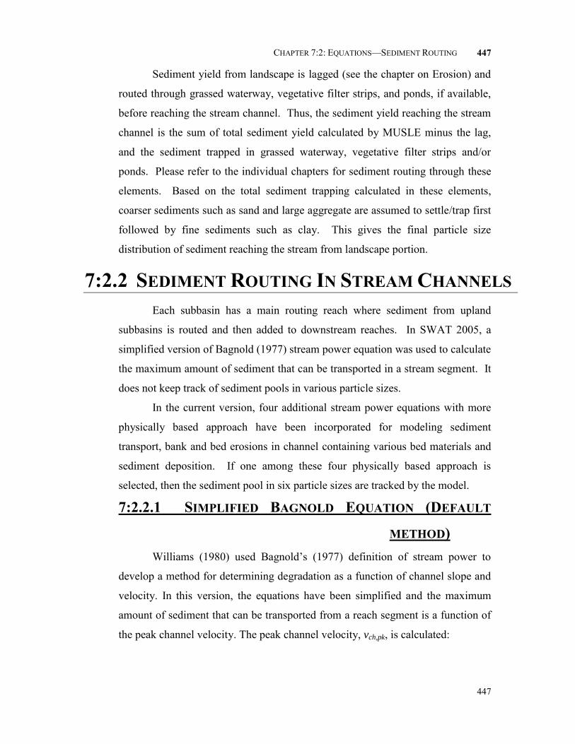
CHAPTER 7:2: EQUATIONS—SEDIMENT ROUTING
447
447
Sediment yield from landscape is lagged (see the chapter on Erosion) and
routed through grassed waterway, vegetative filter strips, and ponds, if available,
before reaching the stream channel. Thus, the sediment yield reaching the stream
channel is the sum of total sediment yield calculated by MUSLE minus the lag,
and the sediment trapped in grassed waterway, vegetative filter strips and/or
ponds. Please refer to the individual chapters for sediment routing through these
elements. Based on the total sediment trapping calculated in these elements,
coarser sediments such as sand and large aggregate are assumed to settle/trap first
followed by fine sediments such as clay. This gives the final particle size
distribution of sediment reaching the stream from landscape portion.
7:2.2 SEDIMENT ROUTING IN STREAM CHANNELS Each subbasin has a main routing reach where sediment from upland
subbasins is routed and then added to downstream reaches. In SWAT 2005, a
simplified version of Bagnold (1977) stream power equation was used to calculate
the maximum amount of sediment that can be transported in a stream segment. It
does not keep track of sediment pools in various particle sizes.
In the current version, four additional stream power equations with more
physically based approach have been incorporated for modeling sediment
transport, bank and bed erosions in channel containing various bed materials and
sediment deposition. If one among these four physically based approach is
selected, then the sediment pool in six particle sizes are tracked by the model.
7:2.2.1 SIMPLIFIED BAGNOLD EQUATION (DEFAULT
METHOD) Williams (1980) used Bagnold’s (1977) definition of stream power to
develop a method for determining degradation as a function of channel slope and
velocity. In this version, the equations have been simplified and the maximum
amount of sediment that can be transported from a reach segment is a function of
the peak channel velocity. The peak channel velocity, vch,pk, is calculated:

448 SWAT THEORETICAL DOCUMENTATION, VERSION 2009
448
ch
pkch
pkchA
qv
,, 7:2.2.1
where qch,pk is the peak flow rate (m3/s) and Ach is the cross-sectional area of flow
in the channel (m2). The peak flow rate is defined as:
chpkch qprfq , 7:2.2.2
where prf is the peak rate adjustment factor, and qch is the average rate of flow
(m3/s). Calculation of the average rate of flow, qch, and the cross-sectional area of
flow, Ach, is reviewed in Section 7, Chapter 1.
The maximum amount of sediment that can be transported from a reach
segment is calculated:
spexp
pkchspmxchsed vcconc ,,, 7:2.2.3
where concsed,ch,mx is the maximum concentration of sediment that can be
transported by the water (ton/m3 or kg/L), csp is a coefficient defined by the user,
vch,pk is the peak channel velocity (m/s), and spexp is an exponent defined by the
user. The exponent, spexp, normally varies between 1.0 and 2.0 and was set at 1.5
in the original Bagnold stream power equation (Arnold et al., 1995).
The maximum concentration of sediment calculated with equation 24.1.3
is compared to the concentration of sediment in the reach at the beginning of the
time step, concsed,ch,i. If mxchsedichsed concconc ,,,, , deposition is the dominant
process in the reach segment and the net amount of sediment deposited is
calculated:
chmxchsedichseddep Vconcconcsed ,,,, 7:2.2.4
where seddep is the amount of sediment deposited in the reach segment (metric
tons), concsed,ch,i is the initial sediment concentration in the reach (kg/L or ton/m3),
concsed,ch,mx is the maximum concentration of sediment that can be transported by
the water (kg/L or ton/m3), and Vch is the volume of water in the reach segment
(m3 H2O).
If mxchsedichsed concconc ,,,, , degradation is the dominant process in the
reach segment and the net amount of sediment reentrained is calculated:
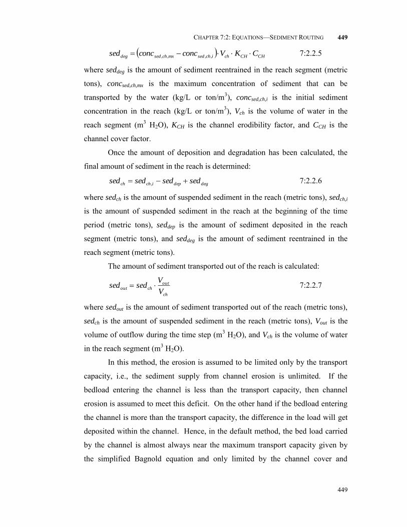
CHAPTER 7:2: EQUATIONS—SEDIMENT ROUTING
449
449
CHCHchichsedmxchseddeg CKVconcconcsed ,,,, 7:2.2.5
where seddeg is the amount of sediment reentrained in the reach segment (metric
tons), concsed,ch,mx is the maximum concentration of sediment that can be
transported by the water (kg/L or ton/m3), concsed,ch,i is the initial sediment
concentration in the reach (kg/L or ton/m3), Vch is the volume of water in the
reach segment (m3 H2O), KCH is the channel erodibility factor, and CCH is the
channel cover factor.
Once the amount of deposition and degradation has been calculated, the
final amount of sediment in the reach is determined:
degdepichch sedsedsedsed , 7:2.2.6
where sedch is the amount of suspended sediment in the reach (metric tons), sedch,i
is the amount of suspended sediment in the reach at the beginning of the time
period (metric tons), seddep is the amount of sediment deposited in the reach
segment (metric tons), and seddeg is the amount of sediment reentrained in the
reach segment (metric tons).
The amount of sediment transported out of the reach is calculated:
ch
outchout
V
Vsedsed 7:2.2.7
where sedout is the amount of sediment transported out of the reach (metric tons),
sedch is the amount of suspended sediment in the reach (metric tons), Vout is the
volume of outflow during the time step (m3 H2O), and Vch is the volume of water
in the reach segment (m3 H2O).
In this method, the erosion is assumed to be limited only by the transport
capacity, i.e., the sediment supply from channel erosion is unlimited. If the
bedload entering the channel is less than the transport capacity, then channel
erosion is assumed to meet this deficit. On the other hand if the bedload entering
the channel is more than the transport capacity, the difference in the load will get
deposited within the channel. Hence, in the default method, the bed load carried
by the channel is almost always near the maximum transport capacity given by
the simplified Bagnold equation and only limited by the channel cover and

450 SWAT THEORETICAL DOCUMENTATION, VERSION 2009
450
erodibility factors (eq. 7:2.2.11). During subsequent floods, the deposited
sediments will be resuspended and transported before channel degradation.
If this method is chosen for sediment transport modeling, it does not keep
track of particle size distribution through the channel reaches and all are assumed
to be of silt size particles. Further, the channel erosion is not partitioned between
stream bank and stream bed and deposition is assumed to occur only in the main
channel; flood plain deposition of sediments is also not modeled separately.
7:2.2.2 PHYSICS BASED APPROACH FOR CHANNEL
EROSION For the channel erosion to occur, both transport and supply should not be
limiting, i.e., 1) the stream power (transport capacity) of the water should be high
and the sediment load from the upstream regions should be less than this capacity
and 2) The shear stress exerted by the water on the bed and bank should be more
than the critical shear stress to dislodge the sediment particle. The potential
erosion rates of bank and bed is predicted based on the excess shear stress
equation (Hanson and Simon, 2001): 6
,,, 10)( bankcbankebankdbank k 7:2.2.8
6,,, 10)( bedcbedebeddbed k 7:2.2.9
where ξ – erosion rates of the bank and bed (m/s), kd – erodibility coefficient of
bank and bed (cm3/N-s) and τc – Critical shear stress acting on bank and bed
(N/m2). This equation indicates that effective stress on the channel bank and bed
should be more than the respective critical stress for the erosion to occur.
The effective shear stress acting on the bank and bed are calculated using
the following equations (Eaton and Millar, 2004):
depth
PWSF
slpdepth
bedbank
ch
banke
4sin)(
100,
7:2.2.10
5.0
21001,
bed
bank
chw
bede
P
WSF
slpdepth
7:2.2.11
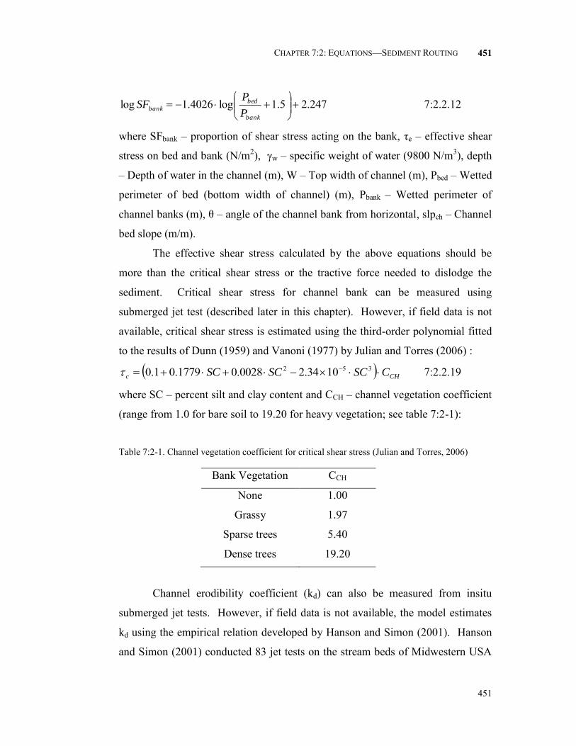
CHAPTER 7:2: EQUATIONS—SEDIMENT ROUTING
451
451
247.25.1log4026.1log
bank
bed
bankP
PSF 7:2.2.12
where SFbank – proportion of shear stress acting on the bank, τe – effective shear
stress on bed and bank (N/m2), γw – specific weight of water (9800 N/m3), depth
– Depth of water in the channel (m), W – Top width of channel (m), Pbed – Wetted
perimeter of bed (bottom width of channel) (m), Pbank – Wetted perimeter of
channel banks (m), θ – angle of the channel bank from horizontal, slpch – Channel
bed slope (m/m).
The effective shear stress calculated by the above equations should be
more than the critical shear stress or the tractive force needed to dislodge the
sediment. Critical shear stress for channel bank can be measured using
submerged jet test (described later in this chapter). However, if field data is not
available, critical shear stress is estimated using the third-order polynomial fitted
to the results of Dunn (1959) and Vanoni (1977) by Julian and Torres (2006) :
CHc CSCSCSC 352 1034.20028.01779.01.0 7:2.2.19
where SC – percent silt and clay content and CCH – channel vegetation coefficient
(range from 1.0 for bare soil to 19.20 for heavy vegetation; see table 7:2-1):
Table 7:2-1. Channel vegetation coefficient for critical shear stress (Julian and Torres, 2006)
Bank Vegetation CCH
None 1.00
Grassy 1.97
Sparse trees 5.40
Dense trees 19.20
Channel erodibility coefficient (kd) can also be measured from insitu
submerged jet tests. However, if field data is not available, the model estimates
kd using the empirical relation developed by Hanson and Simon (2001). Hanson
and Simon (2001) conducted 83 jet tests on the stream beds of Midwestern USA

452 SWAT THEORETICAL DOCUMENTATION, VERSION 2009
452
and established the following relationship between critical shear stress and
erodibility coefficient: 5.02.0
cdk 7:2.2.13
where kd – erodibility coefficient (cm3/N-s) and τc – Critical shear stress (N/m2).
Using the above relationships, the bank/bed erosion rate (m/s) can be
calculated using eqns. 7:2.2.14 and 7:2.2.15. This has to be multiplied by the
sediment bulk density and area exposed to erosion to get the total mass of
sediment that could be eroded. Due to the meandering nature of the channel, the
outside bank in a meander is more prone to erosion than the inside bank. Hence,
the potential bank erosion is calculated by assuming erosion of effectively one
channel bank:
8640011000 ,2 bankbchchbnk ZdepthLBnkrte 7:2.2.14
Similarly, the amount of bed erosion is calculated as:
864001000 , bedbbtmchbed WLBedrte 7:2.2.15
where Bnkrte, Bedrte – potential bank and bed erosion rates (Metric tons per day),
Lch – length of the channel (m), depth – depth of water flowing in the channel
(m), Wbtm – Channel bottom width (m), ρb,bank, ρb,bed – bulk density of channel
bank and bed sediment (g/cm3 or Metric tons/m3 or Mg/m3). The relative erosion
potential is used to partition the erosion in channel among stream bed and stream
bank if the transport capacity of the channel is high. The relative erosion
potential of stream bank and bed is calculated as:
BedrteBnkrte
BnkrteBnk rp
7:2.2.16
rprp BnkBed 1 7:2.2.17
SWAT currently has four stream power models to predict the transport
capacity of channel. The stream power models predict the maximum
concentration of bed load it can carry as a non-linear function of peak velocity:
)(., velocitypeakfconc mxchsed 7:2.2.18

CHAPTER 7:2: EQUATIONS—SEDIMENT ROUTING
453
453
where concsed,ch.mx – maximum concentration of sediment that can be transported
by the water (Metric ton/m3). The stream power models currently used in SWAT
are 1) Simplified Bagnold model 2) Kodatie model (for streams with bed material
size ranging from silt to gravel) 3) Molinas and Wu model (for primarily sand size
particles) and 4) Yang sand and gravel model (for primarily sand and gravel size
particles).
1. Simplified Bagnold model: (same as eqn. 7:2.2.9) spexp
pkchspmxchsed vcconc ,,, 7:2.2.19
where concsed,ch,mx is the maximum concentration of sediment that can be
transported by the water (ton/m3 or kg/L), csp is a coefficient defined by the user,
vch,pk is the peak channel velocity (m/s), and spexp is an exponent defined by the
user. The exponent, spexp, normally varies between 1.0 and 2.0 and was set at 1.5
in the original Bagnold stream power equation (Arnold et al., 1995).
2. Kodatie model
Kodatie (2000) modified the equations developed by Posada (1995) using
nonlinear optimization and field data for different sizes of riverbed sediment.
This method can be used for streams with bed material in size ranging from silt to
gravel:
2.,btm
in
dcb
ch
mxchsed
WW
Q
Syaconc
7:2.2.20
where νch – mean flow velocity (m/s), y – mean flow depth (m), S – Energy slope,
assumed to be the same as bed slope (m/m), (a,b,c and d) – regression coefficients
for different bed materials (Table 7:2-1), Qin – Volume of water entering the reach
in the day (m3), W – width of the channel at the water level (m), Wbtm – bottom
width of the channel (m).
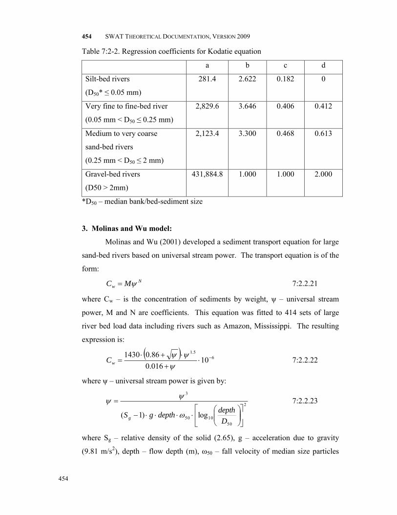
454 SWAT THEORETICAL DOCUMENTATION, VERSION 2009
454
Table 7:2-2. Regression coefficients for Kodatie equation
a b c d
Silt-bed rivers
(D50* ≤ 0.05 mm)
281.4 2.622 0.182 0
Very fine to fine-bed river
(0.05 mm < D50 ≤ 0.25 mm)
2,829.6 3.646 0.406 0.412
Medium to very coarse
sand-bed rivers
(0.25 mm < D50 ≤ 2 mm)
2,123.4 3.300 0.468 0.613
Gravel-bed rivers
(D50 > 2mm)
431,884.8 1.000 1.000 2.000
*D50 – median bank/bed-sediment size
3. Molinas and Wu model:
Molinas and Wu (2001) developed a sediment transport equation for large
sand-bed rivers based on universal stream power. The transport equation is of the
form: N
w MC 7:2.2.21
where Cw – is the concentration of sediments by weight, ψ – universal stream
power, M and N are coefficients. This equation was fitted to 414 sets of large
river bed load data including rivers such as Amazon, Mississippi. The resulting
expression is:
65.1
10016.086.01430
wC 7:2.2.22
where ψ – universal stream power is given by:
2
501050
3
log)1(
D
depthdepthgS g
7:2.2.23
where Sg – relative density of the solid (2.65), g – acceleration due to gravity
(9.81 m/s2), depth – flow depth (m), ω50 – fall velocity of median size particles

CHAPTER 7:2: EQUATIONS—SEDIMENT ROUTING
455
455
(m/s), D50 – median sediment size. The fall velocity is calculated using Stokes’
Law by assuming a temperature of 22ºC and a sediment density of 1.2 t/m3:
3600411 2
5050
D 7:2.2.24
The concentration by weight is converted to concentration by volume and
the maximum bed load concentration in metric tons/m3 is calculated as:
g
gww
wmxchsed S
SCC
Cconc
)1(., 7:2.2.25
4. Yang sand and gravel model
Yang (1996) related total load to excess unit stream power expressed as
the product of velocity and slope. Separate equations were developed for sand
and gravel bed material and solved for sediment concentration in ppm by weight.
The regression equations were developed based on dimensionless combinations of
unit stream power, critical unit stream power, shear velocity, fall velocity,
kinematic viscosity and sediment size. The sand equation, which should be used
for median sizes (D50) less than 2mm is:
505050
*5050
50
*5050
loglog314.0log409.0799.1
log457.0log286.0435.5log
SVSVD
VDC
crch
w
7:2.2.26
and the gravel equation for D50 between 2mm and 10mm:
505050
*5050
50
*5050
loglog282.0log305.0784.2
log816.4log633.0681.6log
SVSVD
VDC
crch
w
7:2.2.27
where Cw – Sediment concentration in parts per million by weight, ω50 – fall
velocity of the median size sediment (m/s), ν – Kinematic viscosity (m2/s), V* -
Shear velocity gRS (m/s), νch – mean channel velocity (m/s), Vcr – Critical
velocity (m/s), and S – Energy slope, assumed to be the same as bed slope (m/m).

456 SWAT THEORETICAL DOCUMENTATION, VERSION 2009
456
From the above equations, Cw in ppm is divided by 106 to convert in to
concentration by weight. Using eq. 7:2.2.32, Cw is converted in to maximum bed
load concentration (concsed,ch,mx) in metric tons/m3.
By using one of the four models discussed above, the maximum sediment
transport capacity of the channel can be calculated. The excess transport capacity
available in the channel is calculated as:
ichsedmxchsedch concconcVSedEx .,., 7:2.2.28
If SedEX is < 0 then the channel does not have the capacity to transport
eroded sediments and hence there will be no bank and bed erosion. If SedEx is >
0 then the channel has the transport capacity to support eroded bank and bed
sediments. Before channel degradation bank erosion, the deposited sediment
during the previous time steps will be resuspended and removed. The excess
transport capacity available after resuspending the deposited sediments is
removed from channel bank and channel bed.
7:2.2.29
7:2.2.30
seddeg = Bankdeg + Beddeg 7:2.2.31
where Bnkdeg – is the amount of bank erosion in metric tons, Beddeg – is the
amount of bed erosion in metric tons, seddeg – is the total channel erosion from
channel bank and bed in metric tons. Particle size contribution from bank erosion
is calculated as:
7:2.2.32
Bnkdeg = SedEX × Bnkrp SedEX × Bnkrp <= Bnkrte
Bnkdeg = Bnkrte SedEX × Bnkrp > Bnkrte
Beddeg = SedEX × Bedrp SedEX × Bedrp <= Bedrte
Beddeg = Bedrte SedEX × Bedrp > Bedrte
Bnksan = Bnkdeg × Bnksanfri
Bnksil = Bnkdeg × Bnksilfri
Bnkcla = Bnkdeg × Bnkclafri
Bnkgra = Bnkdeg × Bnkgrafri

CHAPTER 7:2: EQUATIONS—SEDIMENT ROUTING
457
457
where Bnksan – is the amount of sand eroded from bank in metric tons, Bnksil – is
the amount of silt eroded from bank, Bnkcla – is the amount of clay eroded from
bank, Bnkgra – is the amount of gravel eroded from bank; Bnksanfri, Bnksilfri,
Bnkclafri, and Bnkgrafri – fraction of sand, silt, clay and gravel content of bank in
channel i. Similarly the particle size contribution from bed erosion is also
calculated separately.
The particle size distribution indicated in Table 7:2-3 for bank and bed
sediments is assumed by the model based on the median sediment size (BnkD50,
BedD50) input by the user. If the median sediment size is not specified by the
user, then the model assumed BnkD50 and BedD50 to be 50 micrometer (0.05 mm)
equivalent to the silt size particles.
Table 7:2-3. Particle size distribution assumed by SWAT based on the median
size of bank and bed sediments
Sediment Fraction D50 (in micrometers)
≤ 5 5 to 50 50 to 2000 > 2000
Sand 0.15 0.15 0.65 0.15
Silt 0.15 0.65 0.15 0.15
Clay 0.65 0.15 0.15 0.05
Gravel 0.05 0.05 0.05 0.65
Deposition of bedload sediments in channel is modeled using the
following equations (Einstein 1965; Pemberton and Lara 1971):
depth
Lx
wheree
Pdep
ch
ch
xz
1000055.1
10011 7:2.2.33
where Pdep - is the percentage of sediments (z - sand, silt, clay, and gravel) that
get deposited, Lch – length of the reach (km), ω – fall velocity of the sediment
particles in m/s (eq. 7:2.2.31), vch – mean flow velocity in the reach (m/s), and
depth – is the depth of water in the channel (m). The particle size diameters
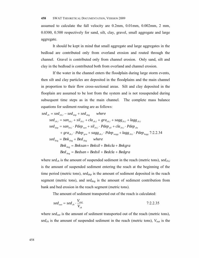
458 SWAT THEORETICAL DOCUMENTATION, VERSION 2009
458
assumed to calculate the fall velocity are 0.2mm, 0.01mm, 0.002mm, 2 mm,
0.0300, 0.500 respectively for sand, silt, clay, gravel, small aggregate and large
aggregate.
It should be kept in mind that small aggregate and large aggregates in the
bedload are contributed only from overland erosion and routed through the
channel. Gravel is contributed only from channel erosion. Only sand, silt and
clay in the bedload is contributed both from overland and channel erosion.
If the water in the channel enters the floodplain during large storm events,
then silt and clay particles are deposited in the floodplains and the main channel
in proportion to their flow cross-sectional areas. Silt and clay deposited in the
flooplain are assumed to be lost from the system and is not resuspended during
subsequent time steps as in the main channel. The complete mass balance
equations for sediment routing are as follows:
BedgraBedclaBedsilBedsanBed
BnkgraBnkclaBnksilBnksanBnk
whereBedBnksed
PdeplaggPdepsaggPdepgra
PdepclaPdepsilPdepsansed
laggsagggraclasilsansed
wheresedsedsedsed
laggichsaggichgraich
claichsilichsanichdep
ichichichichichichich
degdepichch
deg
deg
degdegdeg
,,,
,,,
,,,,,,,
,
7:2.2.34
where sedch is the amount of suspended sediment in the reach (metric tons), sedch,i
is the amount of suspended sediment entering the reach at the beginning of the
time period (metric tons), seddep is the amount of sediment deposited in the reach
segment (metric tons), and seddeg is the amount of sediment contribution from
bank and bed erosion in the reach segment (metric tons).
The amount of sediment transported out of the reach is calculated:
ch
outchout
V
Vsedsed 7:2.2.35
where sedout is the amount of sediment transported out of the reach (metric tons),
sedch is the amount of suspended sediment in the reach (metric tons), Vout is the

CHAPTER 7:2: EQUATIONS—SEDIMENT ROUTING
459
459
volume of outflow during the time step (m3 H2O), and Vch is the volume of water
in the reach segment (m3 H2O).
7:2.3 CHANNEL ERODIBILITY FACTOR The channel erodibility factor is conceptually similar to the soil erodibility
factor used in the USLE equation. Channel erodibility is a function of properties
of the bed or bank materials.
Channel erodibility can be measured with a submerged vertical jet device.
The basic premise of the test is that erosion of a vegetated or bare channel and
local scour beneath an impinging jet are the result of hydraulic stresses, boundary
geometry, and the properties of the material being eroded. Hanson (1990)
developed a method for determining the erodibility coefficient of channels in situ
with the submerged vertical jet. Allen et al. (1999) utilized this method to
determine channel erodibility factors for thirty sites in Texas.
A submerged, vertical jet of water directed perpendicularly at the channel
bed causes erosion of the bed material in the vicinity of the jet impact area (Figure
7:2-1). Important variables in the erosion process are: the volume of material
removed during a jetting event, elevation of the jet above the ground surface,
diameter of the jet nozzle, jet velocity, time, mass density of the fluid and
coefficient of erodibility.
Hanson (1991) defined a jet index, Ji, to relate erodibility to scour created
by the submerged jet. The jet index is a function of the depth of scour beneath the
jet per unit time and the jet velocity. The jet index is determined by a least squares
fit following the procedures outlined in ASTM standard D 5852-95.

460 SWAT THEORETICAL DOCUMENTATION, VERSION 2009
460
Figure 7:2.3-1: Simplified cross-section of submerged jet test (After Allen et al, 1999).
Once the jet index is determined, the channel erodibility coefficient is
calculated:
ibedbankd JK 385exp003.0|, 7:2.3.1
where Kd,bank|bed is the channel bankd/bed erodibility coefficient (cm3/N-s) and Ji
is the jet index. In general, values for channel erodibility are an order of
magnitude smaller than values for soil erodibility.
7:2.4 CHANNEL COVER FACTOR The channel cover factor, CCH, is defined as the ratio of degradation from
a channel with a specified vegetative cover to the corresponding degradation from
a channel with no vegetative cover. The vegetation affects degradation by
reducing the stream velocity, and consequently its erosive power, near the bed
surface.

CHAPTER 7:2: EQUATIONS—SEDIMENT ROUTING
461
461
Table 7:2-1: SWAT input variables that pertain to sediment routing.
Variable Name
Definition Input File
CH_EQN Model used for Channel Erosion 0 – Simplified Bagnold Equation (Default) Physics based approach for channel erosion 1 – Simplified Bagnold Equation 2 – Kodatie model 3 – Molinas and Wu model: 4 – Yang sand and gravel model
.rte
PRF prf: Peak rate adjustment factor (Used only if you choose the simplified Bagnold equation)
.bsn
SPCON csp: Coefficient in sediment transport equation (Used only if you choose the simplified Bagnold equation)
.bsn
SPEXP spexp: Exponent in sediment transport equation (Used only if you choose the simplified Bagnold equation)
.bsn
CH_COV1 If CH_EQN = 1: Kch: Channel erodibility factor (0.0 to 1.0) If CH_EQN ≠ 1: CCH: Channel bank vegetation coefficient as given by table 7:2-1
.rte
CH_COV2 If CH_EQN = 1: CCH: Channel cover factor (0.0 to 1.0) If CH_EQN ≠ 1: CCH: Channel bed vegetation coefficient as given by table 7:2-1
.rte
CH_BNK_BD bankb, : Channel bank bulk density (g/cm3) .rte
CH_BED_BD bedb, : Channel bed bulk density (g/cm3) .rte
CH_BNK_KD Kd,bank: Channel bank erodibility coefficient (cm3/N-s) .rte CH_BED_KD Kd,bed: Channel bed erodibility coefficient (cm3/N-s) .rte CH_BNK_D50 BnkD50: Median particle size diameter of channel bank sediment
(μm) .rte
CH_BED_D50 BedD50: Median particle size diameter of channel bed sediment (μm)
.rte
CH_BNK_TC Τc,bank: Critical shear stress of channel bank (N/m2) .rte
CH_BED_TC Τc,bed: Critical shear stress of channel bed (N/m2) .rte
7:2.5 CHANNEL DOWNCUTTING AND WIDENING
While sediment transport calculations have traditionally been made with
the same channel dimensions throughout a simulation, SWAT will model channel
downcutting and widening. When channel downcutting and widening is
simulated, channel dimensions are allowed to change during the simulation
period.

462 SWAT THEORETICAL DOCUMENTATION, VERSION 2009
462
Three channel dimensions are allowed to vary in channel downcutting and
widening simulations: bankfull depth, depthbnkfull, channel width, Wbnkfull, and
channel slope, slpch. Channel dimensions are updated using the following
equations when the volume of water in the reach exceeds 1.4 106 m3.
The amount of downcutting is calculated (Allen et al., 1999):
CHchdcut Kslpdepthdepth 6.358 7:2.5.1
where depthdcut is the amount of downcutting (m), depth is the depth of water in
channel (m), slpch is the channel slope (m/m), and KCH is the channel erodibility
coefficient (cm/h/Pa).
The new bankfull depth is calculated:
dcutibnkfullbnkfull depthdepthdepth , 7:2.5.2
where depthbnkfull is the new bankfull depth (m), depthbnkfull,i is the previous
bankfull depth, and depthdcut is the amount of downcutting (m).
The new bank width is calculated:
bnkfullWDbnkfull depthratioW 7:2.5.3
where Wbnkfull is the new width of the channel at the top of the bank (m), ratioWD is
the channel width to depth ratio, and depthbnkfull is the new bankfull depth (m).
The new channel slope is calculated:
ch
dcutichch
L
depthslpslp
1000, 7:2.5.4
where slpch is the new channel slope (m/m), slpch,i is the previous channel slope
(m/m), depthbnkfull is the new bankfull depth (m), and Lch is the channel length
(km).
Table 7:2-2: SWAT input variables that pertain to channel downcutting and widening.
Variable Name
Definition Input File
IDEG Channel degradation code .bsn CH_WDR ratioWD: Channel width to depth ratio .rte
CHAPTER 7:2: EQUATIONS—SEDIMENT ROUTING
463
463
7:4.6 NOMENCLATURE Ach Cross-sectional area of flow in the channel (m2) CCH Channel cover factor Ji Jet index used to calculate channel erodibility
KCH Channel erodibility factor (cm/hr/Pa) Lch Channel length (km) Vch Volume of water in the reach segment (m3 H2O) Vout Volume of outflow during the time step (m3 H2O) Wbnkfull Top width of the channel when filled with water (m)
csp Coefficient in sediment transport equation concsed,ch,i Initial sediment concentration in the reach (kg/L or ton/m3) concsed,ch,mx Maximum concentration of sediment that can be transported by the water
(kg/L or ton/m3) depth Depth of water in channel (m) depthbnkfull Depth of water in the channel when filled to the top of the bank (m) depthdcut Amount of downcutting (m) prf Peak rate adjustment factor qch Average rate of flow in the channel (m3/s) qch,pk Peak flow rate (m3/s) ratioWD Channel width to depth ratio
sedch Amount of suspended sediment in the reach (metric tons) seddeg Amount of sediment reentrained in the reach segment (metric tons) seddep Amount of sediment deposited in the reach segment (metric tons) sedout Amount of sediment transported out of the reach (metric tons) slpch Average channel slope along channel length (m m-1) spexp Exponent in sediment transport equation
vch,pk Peak channel velocity (m/s)
464 SWAT THEORETICAL DOCUMENTATION, VERSION 2009
464
7:2.7 REFERENCES
Allen, P.M., J. Arnold, E. Jakubowski. 1999. Prediction of stream channel erosion
potential. Environmental and Engineering Geoscience 5:339-351.
American Society for Testing and Materials. 1995. Annual book of ASTM
standards, Vol. 04.08, Designation: D 5852-5. American Society for
Testing and Materials, Philidelphia, PA. p. 653-657.
Arnold, J.G., J.R. Williams, and D.R. Maidment. 1995. Continuous-time water
and sediment-routing model for large basins. Journal of Hydraulic
Engineering. 121:171-183.
Bagnold, R.A. 1977. Bedload transport in natural rivers. Water Resour. Res.
13:303-312.
Dunn, I.S. 1959. Tractive resistance of cohesive channels. Journal of the Soil
Mechanics and Foundations Division, ASCE 85 (SM 3), 1-24.
Eaton, B. C. and R. G. Millar. 2004. Optimal alluvial channel width under a
bank stability constraint. Geomorphology, 62:35-45.
Einstein, H.A. 1965. Final Report Spawning Grounds. U. of California, Hydr.
Eng. Lab., 16p.
Foster, G.R., L.J. Lane, J.D. Nowlin, J.M. Laflen, and R.A. Young. 1980. A
model to estimate the sediment yield from file-sized areas: Development
of model. CP-80-10. Intl. Inst. For Applied Systems Analysis. A-2361.
Lexenburg, Austria.
Hanson, G.J. 1990. Surface erodibility of earthen channels at high stresses. Part
II-Developing an in situ testing device. Trans. ASAE 33:132-137.
Hanson, G.J. 1991. Development of a jet index method to characterize erosion
resistance of soils in earthen spillways. Trans. ASAE 34:2015-2020.
Hanson, G. J. and A. Simon. 2001. Erodibility of cohesive streambeds in the
loess area of the Midwestern USA. Hydrological Processes, 15:23-38.
Julian, J. P. and R. Torres. 2006. Hydraulic Erosion of Cohesive river banks.
Geomorphology, 76:193-206.
CHAPTER 7:2: EQUATIONS—SEDIMENT ROUTING
465
465
Kodoatie, Robert J. 2000. Sediment transport relations in alluvial channels. Thesis
(Ph. D.)--Colorado State University, 285pp.
Molinas, A. and B. Wu. 2001. Transport of Sediment in large sand-bed rivers.
Journal of Hydraulic research, 39: 135-146.
Pemberton, E. L. and J. M. Lara. 1971. A procedure to determine sediment
deposition in a settling basin. Section E: Intake Works and Desilting
Basins. Sedimentation Section, Division of Planning Coordination,
Bureau of Reclamation, U. S. Department of the Interior.
Posada. 1995. Transport of Sands in Deep Rivers. Thesis (Ph. D.)--Colorado
State University, 158pp.
Vanoni, V.A. (Ed.). 1977. Sedimentation Engineering. ASCE, New York. 745pp.
Williams, J.R. 1980. SPNM, a model for predicting sediment, phosphorus, and
nitrogen yields from agricultural basins. Water Resour. Bull. 16:843-848.
Williams, J.R. and H.D. Berndt. 1977. Sediment yield prediction based on
watershed hydrology. Trans. ASAE 20(6): 1100-1104.
Yang, C. T. 1996. Sediment Transport Theory and practice. The McGraw-Hill
Companies, Inc., New York.

466 SWAT THEORETICAL DOCUMENTATION, VERSION 2009
466

467
SECTION 7 CHAPTER 3
EQUATIONS:
IN-STREAM NUTRIENT PROCESSES
Parameters which affect water quality and can be considered pollution indicators include nutrients, total solids, biological oxygen demand, nitrates, and microorganisms (Loehr, 1970; Paine, 1973). Parameters of secondary importance include odor, taste, and turbidity (Azevedo and Stout, 1974).
The SWAT in-stream water quality algorithms incorporate constituent interactions and relationships used in the QUAL2E model (Brown and Barnwell, 1987). The documentation provided in this chapter has been taken from Brown and Barnwell (1987). The modeling of in-stream nutrient transformations has been made an optional feature of SWAT. To route nutrient loadings downstream without simulating transformations, the variable IWQ in the basin input (.bsn) file should be set to 0. To activate the simulation of in-stream nutrient transformations, this variable should be set to 1.

468 SWAT THEORETICAL DOCUMENTATION, VERSION 2009
468
7:3.1 ALGAE During the day, algae increase the stream’s dissolved oxygen
concentration via photosynthesis. At night, algae reduce the concentration via respiration. As algae grow and die, they form part of the in-stream nutrient cycle. This section summarizes the equations used to simulate algal growth in the stream.
7:3.1.1 CHLOROPHYLL a
Chlorophyll a is assumed to be directly proportional to the concentration of phytoplanktonic algal biomass.
algaechla 0 7:3.1.1
where chla is the chlorophyll a concentration (μg chla/L), 0 is the ratio of chlorophyll a to algal biomass (μg chla/mg alg), and algae is the algal biomass concentration (mg alg/L).
7:3.1.2 ALGAL GROWTH
Growth and decay of algae/chlorophyll a is calculated as a function of the growth rate, the respiration rate, the settling rate and the amount of algae present in the stream. The change in algal biomass for a given day is:
TTalgaedepth
algaealgaealgae aa
1 7:3.1.2
where algae is the change in algal biomass concentration (mg alg/L), a is the
local specific growth rate of algae (day-1 or hr-1), a is the local respiration or
death rate of algae (day-1 or hr-1), 1 is the local settling rate for algae (m/day or m/hr), depth is the depth of water in the channel (m), algae is the algal biomass concentration at the beginning of the day (mg alg/L), and TT is the flow travel time in the reach segment (day or hr). The calculation of depth and travel time are reviewed in Chapter 7:1.
7:3.1.2.1 LOCAL SPECIFIC GROWTH RATE OF ALGAE The local specific growth rate of algae is a function of the
availability of required nutrients, light and temperature. SWAT first
calculates the growth rate at 20C and then adjusts the growth rate for

CHAPTER 7:3: EQUATIONS—IN-STREAM NUTRIENT PROCESSES
469
469
water temperature. The user has three options for calculating the impact of nutrients and light on growth: multiplicative, limiting nutrient, and harmonic mean.
The multiplicative option multiplies the growth factors for light, nitrogen and phosphorus together to determine their net effect on the local algal growth rate. This option has its biological basis in the mutiplicative effects of enzymatic processes involved in photosynthesis:
FPFNFLmaxa 20, 7:3.1.3
where a,20 is the local specific algal growth rate at 20C (day-1 or hr-1),
max is the maximum specific algal growth rate (day-1 or hr-1), FL is the algal growth attenuation factor for light, FN is the algal growth limitation factor for nitrogen, and FP is the algal growth limitation factor for phosphorus. The maximum specific algal growth rate is specified by the user. The limiting nutrient option calculates the local algal growth rate as limited by light and either nitrogen or phosphorus. The nutrient/light effects are multiplicative, but the nutrient/nutrient effects are alternate. The algal growth rate is controlled by the nutrient with the smaller growth limitation factor. This approach mimics Liebig’s law of the minimum:
FPFNFLmaxa ,min20, 7:3.1.4
where a,20 is the local specific algal growth rate at 20C (day-1 or hr-1),
max is the maximum specific algal growth rate (day-1 or hr-1), FL is the algal growth attenuation factor for light, FN is the algal growth limitation factor for nitrogen, and FP is the algal growth limitation factor for phosphorus. The maximum specific algal growth rate is specified by the user. The harmonic mean is mathematically analogous to the total resistance of two resistors in parallel and can be considered a compromise between equations 7:3.1.3 and 7:3.1.4. The algal growth rate is controlled by a multiplicative relation between light and nutrients, while the nutrient/nutrient interactions are represented by a harmonic mean.

470 SWAT THEORETICAL DOCUMENTATION, VERSION 2009
470
FPFN
FLmaxa 112
20, 7:3.1.5
where a,20 is the local specific algal growth rate at 20C (day-1 or hr-1),
max is the maximum specific algal growth rate (day-1 or hr-1), FL is the algal growth attenuation factor for light, FN is the algal growth limitation factor for nitrogen, and FP is the algal growth limitation factor for phosphorus. The maximum specific algal growth rate is specified by the user. Calculation of the growth limiting factors for light, nitrogen and phosphorus are reviewed in the following sections.
ALGAL GROWTH LIMITING FACTOR FOR LIGHT. A number of mathematical relationships between
photosynthesis and light have been developed. All relationships show an increase in photosynthetic rate with increasing light intensity up to a maximum or saturation value. The algal growth limiting factor for light is calculated using a Monod half-saturation method. In this option, the algal growth limitation factor for light is defined by a Monod expression:
zphosynL
zphosyn
zIK
IFL
,
,
7:3.1.6
where FLz is the algal growth attenuation factor for light at depth z, Iphosyn,z is the photosynthetically-active light intensity at a depth z below the water surface (MJ/m2-hr), and KL is the half-saturation coefficient for light (MJ/m2-hr). Photosynthetically-active light is radiation with a wavelength between 400 and 700 nm. The half-saturation coefficient for light is defined as the light intensity at which the algal growth rate is 50% of the maximum growth rate. The half-saturation coefficient for light is defined by the user. Photosynthesis is assumed to occur throughout the depth of the water column. The variation in light intensity with depth is defined by Beer’s law:
zkII hrphosynzphosyn exp,, 7:3.1.7

CHAPTER 7:3: EQUATIONS—IN-STREAM NUTRIENT PROCESSES
471
471
where Iphosyn,z is the photosynthetically-active light intensity at a depth z below the water surface (MJ/m2-hr), Iphosyn,hr is the photosynthetically-active solar radiation reaching the ground/water
surface during a specific hour on a given day (MJ/m2-hr), k is the
light extinction coefficient (m-1), and z is the depth from the water surface (m). Substituting equation 7:3.1.7 into equation 7:3.1.6 and integrating over the depth of flow gives:
depthkIK
IK
depthkFL
hrphosynL
hrphosynL
expln1
,
, 7:3.1.8
where FL is the algal growth attenuation factor for light for the water column, KL is the half-saturation coefficient for light (MJ/m2-hr), Iphosyn,hr is the photosynthetically-active solar radiation reaching the ground/water surface during a specific hour on a
given day (MJ/m2-hr), k is the light extinction coefficient (m-1),
and depth is the depth of water in the channel (m). Equation 7:3.1.8 is used to calculated FL for hourly routing. The photosynthetically-active solar radiation is calculated:
phosynhrhrphosyn frII , 7:3.1.9
where Ihr is the solar radiation reaching the ground during a specific hour on current day of simulation (MJ m-2 h-1), and frphosyn is the fraction of solar radiation that is photosynthetically active. The calculation of Ihr is reviewed in Chapter 1:1. The fraction of solar radiation that is photosynthetically active is user defined. For daily simulations, an average value of the algal growth attenuation factor for light calculated over the diurnal cycle must be used. This is calculated using a modified form of equation 7:3.1.8:
depthkIK
IK
depthkfrFL
hrphosynL
hrphosynL
DL
expln192.0
,
, 7:3.1.10
where frDL is the fraction of daylight hours, hrphosynI , is the daylight
average photosynthetically-active light intensity (MJ/m2-hr) and all
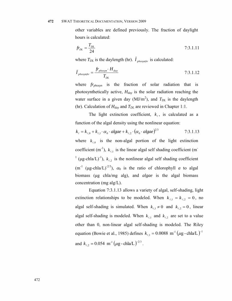
472 SWAT THEORETICAL DOCUMENTATION, VERSION 2009
472
other variables are defined previously. The fraction of daylight hours is calculated:
24DL
DL
Tfr 7:3.1.11
where TDL is the daylength (hr). hrphosynI , is calculated:
DL
dayphosyn
hrphosynT
HfrI
, 7:3.1.12
where frphosyn is the fraction of solar radiation that is photosynthetically active, Hday is the solar radiation reaching the water surface in a given day (MJ/m2), and TDL is the daylength (hr). Calculation of Hday and TDL are reviewed in Chapter 1:1.
The light extinction coefficient, k , is calculated as a
function of the algal density using the nonlinear equation:
3202,01,0, algaekalgaekkk 7:3.1.13
where 0,k is the non-algal portion of the light extinction
coefficient (m-1), 1,k is the linear algal self shading coefficient (m-
1 (μg-chla/L)-1), 2,k is the nonlinear algal self shading coefficient
(m-1 (μg-chla/L)-2/3), 0 is the ratio of chlorophyll a to algal biomass (μg chla/mg alg), and algae is the algal biomass concentration (mg alg/L). Equation 7:3.1.13 allows a variety of algal, self-shading, light
extinction relationships to be modeled. When 02,1, kk , no
algal self-shading is simulated. When 01, k and 02, k , linear
algal self-shading is modeled. When 1,k and 2,k are set to a value
other than 0, non-linear algal self-shading is modeled. The Riley
equation (Bowie et al., 1985) defines 1-11, chla/L-g m 0088.0 k
and 32-12, chla/L-g m 054.0 k .

CHAPTER 7:3: EQUATIONS—IN-STREAM NUTRIENT PROCESSES
473
473
ALGAL GROWTH LIMITING FACTOR FOR NUTRIENTS. The algal growth limiting factor for nitrogen is defined by a
Monod expression. Algae are assumed to use both ammonia and nitrate as a source of inorganic nitrogen.
NNHNO
NHNO
KCC
CCFN
43
43 7:3.1.14
where FN is the algal growth limitation factor for nitrogen, CNO3 is the concentration of nitrate in the reach (mg N/L), CNH4 is the concentration of ammonium in the reach (mg N/L), and KN is the Michaelis-Menton half-saturation constant for nitrogen (mg N/L).
The algal growth limiting factor for phosphorus is also defined by a Monod expression.
PsolP
solP
KC
CFP
7:3.1.15
where FP is the algal growth limitation factor for phosphorus, CsolP is the concentration of phosphorus in solution in the reach (mg P/L), and KP is the Michaelis-Menton half-saturation constant for phosphorus (mg P/L). The Michaelis-Menton half-saturation constant for nitrogen and phosphorus define the concentration of N or P at which algal growth is limited to 50% of the maximum growth rate. Users are allowed to set these values. Typical values for KN range from 0.01 to 0.30 mg N/L while KP will range from 0.001 to 0.05 mg P/L.
Once the algal growth rate at 20C is calculated, the rate coefficient is adjusted for temperature effects using a Streeter-Phelps type formulation:
2020, 047.1 waterT
aa 7:3.1.16
where a is the local specific growth rate of algae (day-1 or hr-1), a,20 is
the local specific algal growth rate at 20C (day-1 or hr-1), and Twater is the
average water temperature for the day or hour (C).

474 SWAT THEORETICAL DOCUMENTATION, VERSION 2009
474
7:3.1.2.2 LOCAL RESPIRATION RATE OF ALGAE The local respiration or death rate of algae represents the net effect
of three processes: the endogenous respiration of algae, the conversion of algal phosphorus to organic phosphorus, and the conversion of algal nitrogen to organic nitrogen. The user defines the local respiration rate of
algae at 20C. The respiration rate is adjusted to the local water temperature using the relationship:
2020, 047.1 waterT
aa 7:3.1.17
where a is the local respiration rate of algae (day-1 or hr-1), a,20 is the
local algal respiration rate at 20C (day-1 or hr-1), and Twater is the average
water temperature for the day or hour (C).
7:3.1.2.3 LOCAL SETTLING RATE OF ALGAE The local settling rate of algae represents the net removal of algae
due to settling. The user defines the local settling rate of algae at 20C. The settling rate is adjusted to the local water temperature using the relationship:
2020,11 024.1 waterT 7:3.1.18
where 1 is the local settling rate of algae (m/day or m/hr), 1,20 is the
local algal settling rate at 20C (m/day or m/hr), and Twater is the average
water temperature for the day or hour (C).
Table 7:3-1: SWAT input variables used in algae calculations. Variable
name
Definition File
Name AI0 0: Ratio of chlorophyll a to algal biomass (μg chla/mg alg) .wwq IGROPT Algal specific growth rate option .wwq MUMAX max: Maximum specific algal growth rate (day-1) .wwq K_L KL: Half-saturation coefficient for light (MJ/m2-hr) .wwq TFACT frphosyn: Fraction of solar radiation that is photosynthetically active .wwq LAMBDA0
0,k : Non-algal portion of the light extinction coefficient (m-1) .wwq
LAMBDA1 1,k : Linear algal self shading coefficient (m-1 (μg-chla/L)-1) .wwq
LAMBDA2 2,k : Nonlinear algal self shading coefficient (m-1 (μg-chla/L)-2/3) .wwq
K_N KN: Michaelis-Menton half-saturation constant for nitrogen (mg N/L) .wwq K_P KP: Michaelis-Menton half-saturation constant for phosphorus (mg P/L) .wwq RHOQ a,20: Local algal respiration rate at 20C (day-1) .wwq RS1 1,20: Local algal settling rate at 20C (m/day) .swq

CHAPTER 7:3: EQUATIONS—IN-STREAM NUTRIENT PROCESSES
475
475
7:3.2 NITROGEN CYCLE
In aerobic water, there is a stepwise transformation from organic nitrogen to ammonia, to nitrite, and finally to nitrate. Organic nitrogen may also be removed from the stream by settling. This section summarizes the equations used to simulate the nitrogen cycle in the stream.
7:3.2.1 ORGANIC NITROGEN
The amount of organic nitrogen in the stream may be increased by the conversion of algal biomass nitrogen to organic nitrogen. Organic nitrogen concentration in the stream may be decreased by the conversion of organic nitrogen to NH4
+ or the settling of organic nitrogen with sediment. The change in organic nitrogen for a given day is:
TTorgNorgNalgaeorgN strstrNastr 43,1 7:3.2.1
where orgNstr is the change in organic nitrogen concentration (mg N/L), 1 is the
fraction of algal biomass that is nitrogen (mg N/mg alg biomass), a is the local respiration or death rate of algae (day-1 or hr-1), algae is the algal biomass
concentration at the beginning of the day (mg alg/L), N,3 is the rate constant for hydrolysis of organic nitrogen to ammonia nitrogen (day-1 or hr-1), orgNstr is the
organic nitrogen concentration at the beginning of the day (mg N/L), 4 is the rate coefficient for organic nitrogen settling (day-1 or hr-1), and TT is the flow travel time in the reach segment (day or hr). The fraction of algal biomass that is nitrogen is user-defined. Equation 7:3.1.17 describes the calculation of the local respiration rate of algae. The calculation of travel time is reviewed in Chapter 7:1. The user defines the local rate constant for hydrolysis of organic nitrogen
to NH4+ at 20C. The organic nitrogen hydrolysis rate is adjusted to the local
water temperature using the relationship: 20
20,3,3, 047.1 waterT
NN 7:3.2.2
where N,3 is the local rate constant for hydrolysis of organic nitrogen to NH4+
(day-1 or hr-1), N,3,20 is the local rate constant for hydrolysis of organic nitrogen to
NH4+ at 20C (day-1 or hr-1), and Twater is the average water temperature for the
day or hour (C).

476 SWAT THEORETICAL DOCUMENTATION, VERSION 2009
476
The user defines the rate coefficient for organic nitrogen settling at 20C. The organic nitrogen settling rate is adjusted to the local water temperature using the relationship:
2020,44 024.1 waterT 7:3.2.3
where 4 is the local settling rate for organic nitrogen (day-1 or hr-1), 4,20 is the
local settling rate for organic nitrogen at 20C (day-1 or hr-1), and Twater is the
average water temperature for the day or hour (C).
7:3.2.2 AMMONIUM
The amount of ammonium (NH4+) in the stream may be increased by the
mineralization of organic nitrogen and diffusion of ammonium from the streambed sediments. The ammonium concentration in the stream may be
decreased by the conversion of NH4+ to -
2NO or the uptake of NH4+ by algae. The
change in ammonium for a given day is:
TTalgaefr
depthNH4orgNNH4 aNHstrNstrNstr
14
31,3, 1000
7:3.2.4
where NH4str is the change in ammonium concentration (mg N/L), N,3 is the rate constant for hydrolysis of organic nitrogen to ammonia nitrogen (day-1 or hr-
1), orgNstr is the organic nitrogen concentration at the beginning of the day (mg
N/L), N,1 is the rate constant for biological oxidation of ammonia nitrogen (day-1 or hr-1), NH4str is the ammonium concentration at the beginning of the day (mg
N/L), 3 is the benthos (sediment) source rate for ammonium (mg N/m2-day or mg N/m2-hr), depth is the depth of water in the channel (m), frNH4 is the fraction
of algal nitrogen uptake from ammonium pool, 1 is the fraction of algal biomass
that is nitrogen (mg N/mg alg biomass), a is the local growth rate of algae (day-1 or hr-1), algae is the algal biomass concentration at the beginning of the day (mg alg/L), and TT is the flow travel time in the reach segment (day or hr). The local rate constant for hydrolysis of organic nitrogen to NH4
+ is calculated with equation 7:3.2.2. Section 7:3.1.2.1 describes the calculation of the local growth rate of algae. The calculation of depth and travel time is reviewed in Chapter 7:1.

CHAPTER 7:3: EQUATIONS—IN-STREAM NUTRIENT PROCESSES
477
477
The rate constant for biological oxidation of ammonia nitrogen will vary as a function of in-stream oxygen concentration and temperature. The rate constant is calculated:
2020,1,1, 083.16.0exp1
waterT
strNN Ox 7:3.2.5
where N,1 is the rate constant for biological oxidation of ammonia nitrogen (day-1
or hr-1), N,1,20 is the rate constant for biological oxidation of ammonia nitrogen at
20C (day-1 or hr-1), Oxstr is the dissolved oxygen concentration in the stream (mg
O2/L), and Twater is the average water temperature for the day or hour (C). The
second term on the right side of equation 7:3.2.5, strOx 6.0exp1 , is a
nitrification inhibition correction factor. This factor inhibits nitrification at low dissolved oxygen concentrations.
The user defines the benthos source rate for ammonium at 20C. The benthos source rate for ammonium nitrogen is adjusted to the local water temperature using the relationship:
2020,33 074.1 waterT 7:3.2.6
where 3 is the benthos (sediment) source rate for ammonium (mg N/m2-day or
mg N/m2-hr), 3,20 is the benthos (sediment) source rate for ammonium nitrogen
at 20C (mg N/m2-day or mg N/m2-hr), and Twater is the average water
temperature for the day or hour (C). The fraction of algal nitrogen uptake from ammonium pool is calculated:
strNHstrNH
strNHNH
NO3fNH4f
NH4ffr
44
44 1
7:3.2.7
where frNH4 is the fraction of algal nitrogen uptake from ammonium pool, fNH4 is the preference factor for ammonia nitrogen, NH4str is the ammonium concentration in the stream (mg N/L), and NO3str is the nitrate concentration in the stream (mg N/L).
7:3.2.3 NITRITE
The amount of nitrite ( -2NO ) in the stream will be increased by the
conversion of NH4+ to -
2NO and decreased by the conversion of -2NO to -
3NO .
The conversion of -2NO to -
3NO occurs more rapidly than the conversion of NH4+

478 SWAT THEORETICAL DOCUMENTATION, VERSION 2009
478
to -2NO , so the amount of nitrite present in the stream is usually very small. The
change in nitrite for a given day is:
TTNO2NH4NO2 strNstrNstr 2,1, 7:3.2.8
where NO2str is the change in nitrite concentration (mg N/L), N,1 is the rate constant for biological oxidation of ammonia nitrogen (day-1 or hr-1), NH4str is the
ammonium concentration at the beginning of the day (mg N/L), N,2 is the rate constant for biological oxidation of nitrite to nitrate (day-1 or hr-1), NO2str is the nitrite concentration at the beginning of the day (mg N/L), and TT is the flow travel time in the reach segment (day or hr). The local rate constant for biological oxidation of ammonia nitrogen is calculated with equation 7:3.2.5. The calculation of travel time is reviewed in Chapter 7:1. The rate constant for biological oxidation of nitrite to nitrate will vary as a function of in-stream oxygen concentration and temperature. The rate constant is calculated:
2020,2,2, 047.16.0exp1
waterT
strNN Ox 7:3.2.9
where N,2 is the rate constant for biological oxidation of nitrite to nitrate (day-1 or
hr-1), N,2,20 is the rate constant for biological oxidation of nitrite to nitrate at 20C (day-1 or hr-1), Oxstr is the dissolved oxygen concentration in the stream (mg
O2/L), and Twater is the average water temperature for the day or hour (C). The
second term on the right side of equation 7:3.2.9, strOx 6.0exp1 , is a
nitrification inhibition correction factor. This factor inhibits nitrification at low dissolved oxygen concentrations.
7:3.2.4 NITRATE
The amount of nitrate ( -3NO ) in the stream may be increased by the
oxidation of -2NO . The nitrate concentration in the stream may be decreased by
the uptake of -3NO by algae. The change in nitrate for a given day is:
TTalgaefrNO2NO3 aNHstrNstr 142, 1 7:3.2.10
where NO3str is the change in nitrate concentration (mg N/L), N,2 is the rate constant for biological oxidation of nitrite to nitrate (day-1 or hr-1), NO2str is the nitrite concentration at the beginning of the day (mg N/L), frNH4 is the fraction of

CHAPTER 7:3: EQUATIONS—IN-STREAM NUTRIENT PROCESSES
479
479
algal nitrogen uptake from ammonium pool, 1 is the fraction of algal biomass
that is nitrogen (mg N/mg alg biomass), a is the local growth rate of algae (day-1 or hr-1), algae is the algal biomass concentration at the beginning of the day (mg alg/L), and TT is the flow travel time in the reach segment (day or hr). The local rate constant for biological oxidation of nitrite to nitrate is calculated with equation 7:3.2.9 while the fraction of algal nitrogen uptake from ammonium pool is calculated with equation 7:3.2.7. Section 7:3.1.2.1 describes the calculation of the local growth rate of algae. The calculation of travel time is reviewed in Chapter 7:1.
Table 7:3-2: SWAT input variables used in in-stream nitrogen calculations. Variable
name
Definition File
Name AI1 1: Fraction of algal biomass that is nitrogen (mg N/mg alg biomass) .wwq RHOQ a,20: Local algal respiration rate at 20C (day-1) .wwq BC3 N,3,20: Local rate constant for hydrolysis of organic nitrogen to NH4
+ at 20C (day-1 or hr-1)
.swq
RS4 4,20: Local settling rate for organic nitrogen at 20C (day-1) .swq BC1 N,1,20: Rate constant for biological oxidation of ammonia nitrogen at 20C
(day-1) .swq
RS3 3,20: Benthos (sediment) source rate for ammonium nitrogen at 20C (mg N/m2-day or mg N/m2-hr)
.swq
P_N fNH4: Preference factor for ammonia nitrogen .wwq BC2 N,2,20: Rate constant for biological oxidation of nitrite to nitrate at 20C
(day-1 or hr-1) .swq
7:3.3 PHOSPHORUS CYCLE
The phosphorus cycle is similar to the nitrogen cycle. The death of algae transforms algal phosphorus into organic phosphorus. Organic phosphorus is mineralized to soluble phosphorus which is available for uptake by algae. Organic phosphorus may also be removed from the stream by settling. This section summarizes the equations used to simulate the phosphorus cycle in the stream.
7:3.3.1 ORGANIC PHOSPHORUS
The amount of organic phosphorus in the stream may be increased by the conversion of algal biomass phosphorus to organic phosphorus. Organic phosphorus concentration in the stream may be decreased by the conversion of organic phosphorus to soluble inorganic phosphorus or the settling of organic phosphorus with sediment. The change in organic phosphorus for a given day is:

480 SWAT THEORETICAL DOCUMENTATION, VERSION 2009
480
TTorgPorgPalgaeorgP strstrPastr 54,2 7:3.3.1
where orgPstr is the change in organic phosphorus concentration (mg P/L), 2 is
the fraction of algal biomass that is phosphorus (mg P/mg alg biomass), a is the local respiration or death rate of algae (day-1 or hr-1), algae is the algal biomass
concentration at the beginning of the day (mg alg/L), P,4 is the rate constant for mineralization of organic phosphorus (day-1 or hr-1), orgPstr is the organic
phosphorus concentration at the beginning of the day (mg P/L), 5 is the rate coefficient for organic phosphorus settling (day-1 or hr-1), and TT is the flow travel time in the reach segment (day or hr). The fraction of algal biomass that is phosphorus is user-defined. Equation 7:3.1.17 describes the calculation of the local respiration rate of algae. The calculation of travel time is reviewed in Chapter 7:1. The user defines the local rate constant for mineralization of organic
phosphorus at 20C. The organic phosphorus mineralization rate is adjusted to the local water temperature using the relationship:
2020,4,4, 047.1 waterT
PP 7:3.3.2
where P,4 is the local rate constant for organic phosphorus mineralization (day-1
or hr-1), P,4,20 is the local rate constant for organic phosphorus mineralization at
20C (day-1 or hr-1), and Twater is the average water temperature for the day or hour
(C). The user defines the rate coefficient for organic phosphorus settling at
20C. The organic phosphorus settling rate is adjusted to the local water temperature using the relationship:
2020,55 024.1 waterT 7:3.3.3
where 5 is the local settling rate for organic phosphorus (day-1 or hr-1), 5,20 is the
local settling rate for organic phosphorus at 20C (day-1 or hr-1), and Twater is the
average water temperature for the day or hour (C).
7:3.3.2 INORGANIC/SOLUBLE PHOSPHORUS
The amount of soluble, inorganic phosphorus in the stream may be increased by the mineralization of organic phosphorus and diffusion of inorganic phosphorus from the streambed sediments. The soluble phosphorus concentration

CHAPTER 7:3: EQUATIONS—IN-STREAM NUTRIENT PROCESSES
481
481
in the stream may be decreased by the uptake of inorganic P by algae. The change in soluble phosphorus for a given day is:
TTalgae
depthorgPsolP astrPstr
2
24, 1000
7:3.3.4
where solPstr is the change in solution phosphorus concentration (mg P/L), P,4 is the rate constant for mineralization of organic phosphorus (day-1 or hr-1), orgPstr
is the organic phosphorus concentration at the beginning of the day (mg P/L), 2 is the benthos (sediment) source rate for soluble P (mg P/m2-day or mg P/m2-hr),
depth is the depth of water in the channel (m), 2 is the fraction of algal biomass
that is phosphorus (mg P/mg alg biomass), a is the local growth rate of algae (day-1 or hr-1), algae is the algal biomass concentration at the beginning of the day (mg alg/L), and TT is the flow travel time in the reach segment (day or hr). The local rate constant for mineralization of organic phosphorus is calculated with equation 7:3.3.2. Section 7:3.1.2.1 describes the calculation of the local growth rate of algae. The calculation of depth and travel time is reviewed in Chapter 7:1.
The user defines the benthos source rate for soluble P at 20C. The benthos source rate for soluble phosphorus is adjusted to the local water temperature using the relationship:
2020,22 074.1 waterT 7:3.3.5
where 2 is the benthos (sediment) source rate for soluble P (mg P/m2-day or mg
P/m2-hr), 2,20 is the benthos (sediment) source rate for soluble phosphorus at
20C (mg P/m2-day or mg P/m2-hr), and Twater is the average water temperature
for the day or hour (C).
Table 7:3-3: SWAT input variables used in in-stream phosphorus calculations. Variable
name
Definition File
Name AI2 2: Fraction of algal biomass that is phosphorus (mg P/mg alg biomass) .wwq RHOQ a,20: Local algal respiration rate at 20C (day-1) .wwq BC4 P,4,20: Local rate constant for organic phosphorus mineralization at 20C
(day-1) .swq
RS5 5,20: Local settling rate for organic phosphorus at 20C (day-1) .swq RS2 2,20: Benthos (sediment) source rate for soluble phosphorus at 20C (mg
P/m2-day) .swq

482 SWAT THEORETICAL DOCUMENTATION, VERSION 2009
482
7:3.4 CARBONACEOUS BIOLOGICAL OXYGEN DEMAND
The carbonaceous oxygen demand (CBOD) of the water is the amount of
oxygen required to decompose the organic material in the water. CBOD is added
to the stream with loadings from surface runoff or point sources. Within the
stream, two processes are modeled that impact CBOD levels, both of which serve
to reduce the carbonaceous biological oxygen demand as the water moves
downstream. The change in CBOD within the stream on a given day is calculated:
TTcbodcbodcbod 31 7:3.4.1
where cbod is the change in carbonaceous biological oxygen demand
concentration (mg CBOD/L), 1 is the CBOD deoxygenation rate (day-1 or hr-1),
cbod is the carbonaceous biological oxygen demand concentration (mg CBOD/L),
3 is the settling loss rate of CBOD (day-1 or hr-1), and TT is the flow travel time
in the reach segment (day or hr). The calculation of travel time is reviewed in
Chapter 7:1.
The user defines the carbonaceous deoxygenation rate at 20C. The
CBOD deoxygenation rate is adjusted to the local water temperature using the
relationship: 20
20,11 047.1 waterT 7:3.4.2
where 1 is the CBOD deoxygenation rate (day-1 or hr-1), 1,20 is the CBOD
deoxygenation rate at 20C (day-1 or hr-1), and Twater is the average water
temperature for the day or hour (C).
The user defines the settling loss rate of CBOD at 20C. The settling loss
rate is adjusted to the local water temperature using the relationship: 20
20,33 024.1 waterT 7:3.4.3
where 3 is the settling loss rate of CBOD (day-1 or hr-1), 3,20 is the settling loss
rate of CBOD at 20C (day-1 or hr-1), and Twater is the average water temperature
for the day or hour (C).

CHAPTER 7:3: EQUATIONS—IN-STREAM NUTRIENT PROCESSES
483
483
Table 7:3-4: SWAT input variables used in in-stream CBOD calculations.
Variable name
Definition File
Name RK1 1,20: CBOD deoxygenation rate at 20C (day-1) .swq RK3 3,20: Settling loss rate of CBOD at 20C (day-1) .swq
7:3.5 OXYGEN An adequate dissolved oxygen concentration is a basic requirement for a
healthy aquatic ecosystem. Dissolved oxygen concentrations in streams are a
function of atmospheric reareation, photosynthesis, plant and animal respiration,
benthic (sediment) demand, biochemical oxygen demand, nitrification, salinity,
and temperature. The change in dissolved oxygen concentration on a given day is
calculated:
depth
cbodalgaeOxOxOx aastrsatstr
1000
( 41432
TTNO2NH4 strNstrN )2,61,5 7:3.5.1
where Oxstr is the change in dissolved oxygen concentration (mg O2/L), 2 is the
reaeration rate for Fickian diffusion (day-1 or hr-1), Oxsat is the saturation oxygen
concentration (mg O2/L), Oxstr is the dissolved oxygen concentration in the stream
(mg O2/L), 3 is the rate of oxygen production per unit of algal photosynthesis
(mg O2/mg alg), a is the local specific growth rate of algae (day-1 or hr-1), 4 is
the rate of oxygen uptake per unit of algae respired (mg O2/mg alg), a is the local
respiration or death rate of algae (day-1 or hr-1), algae is the algal biomass
concentration at the beginning of the day (mg alg/L), 1 is the CBOD
deoxygenation rate (day-1 or hr-1), cbod is the carbonaceous biological oxygen
demand concentration (mg CBOD/L), 4 is the sediment oxygen demand rate (mg
O2/(m2day) or mg O2/(m2
hr)), depth is the depth of water in the channel (m), 5
is the rate of oxygen uptake per unit NH4+ oxidation (mg O2/mg N), N,1 is the
rate constant for biological oxidation of ammonia nitrogen (day-1 or hr-1), NH4str
is the ammonium concentration at the beginning of the day (mg N/L), 6 is the

484 SWAT THEORETICAL DOCUMENTATION, VERSION 2009
484
rate of oxygen uptake per unit -2NO oxidation (mg O2/mg N), N,2 is the rate
constant for biological oxidation of nitrite to nitrate (day-1 or hr-1), NO2str is the
nitrite concentration at the beginning of the day (mg N/L) and TT is the flow
travel time in the reach segment (day or hr). The user defines the rate of oxygen
production per unit algal photosynthesis, the rate of oxygen uptake per unit algal
respiration, the rate of oxygen uptake per unit NH4+ oxidation and rate of oxygen
uptake per unit -2NO oxidation. Section 7:3.1.2.1 describes the calculation of the
local growth rate of algae while equation 7:3.1.17 describes the calculation of the
local respiration rate of algae. The rate constant for biological oxidation of NH4+
is calculated with equation 7:3.2.5 while the rate constant for -2NO oxidation is
determined with equation 7:3.2.9. The CBOD deoxygenation rate is calculated
using equation 7:3.4.2. The calculation of depth and travel time are reviewed in
Chapter 7:1.
The user defines the sediment oxygen demand rate at 20C. The sediment
oxygen demand rate is adjusted to the local water temperature using the
relationship: 20
20,44 060.1 waterT 7:3.5.2
where 4 is the sediment oxygen demand rate (mg O2/(m2day) or mg O2/(m2
hr)),
4,20 is the sediment oxygen demand rate at 20C (mg O2/(m2day) or mg
O2/(m2hr)), and Twater is the average water temperature for the day or hour (C).
7:3.5.1 OXYGEN SATURATION CONCENTRATION
The amount of oxygen that can be dissolved in water is a function of
temperature, concentration of dissolved solids, and atmospheric pressure. An
equation developed by APHA (1985) is used to calculate the saturation
concentration of dissolved oxygen:
2,
7
,
5 10642308.610575701.134410.139expKwatKwat
satTT
Ox
4
,
11
3,
10 10621949.810243800.1
KwatKwat TT 7:3.5.3
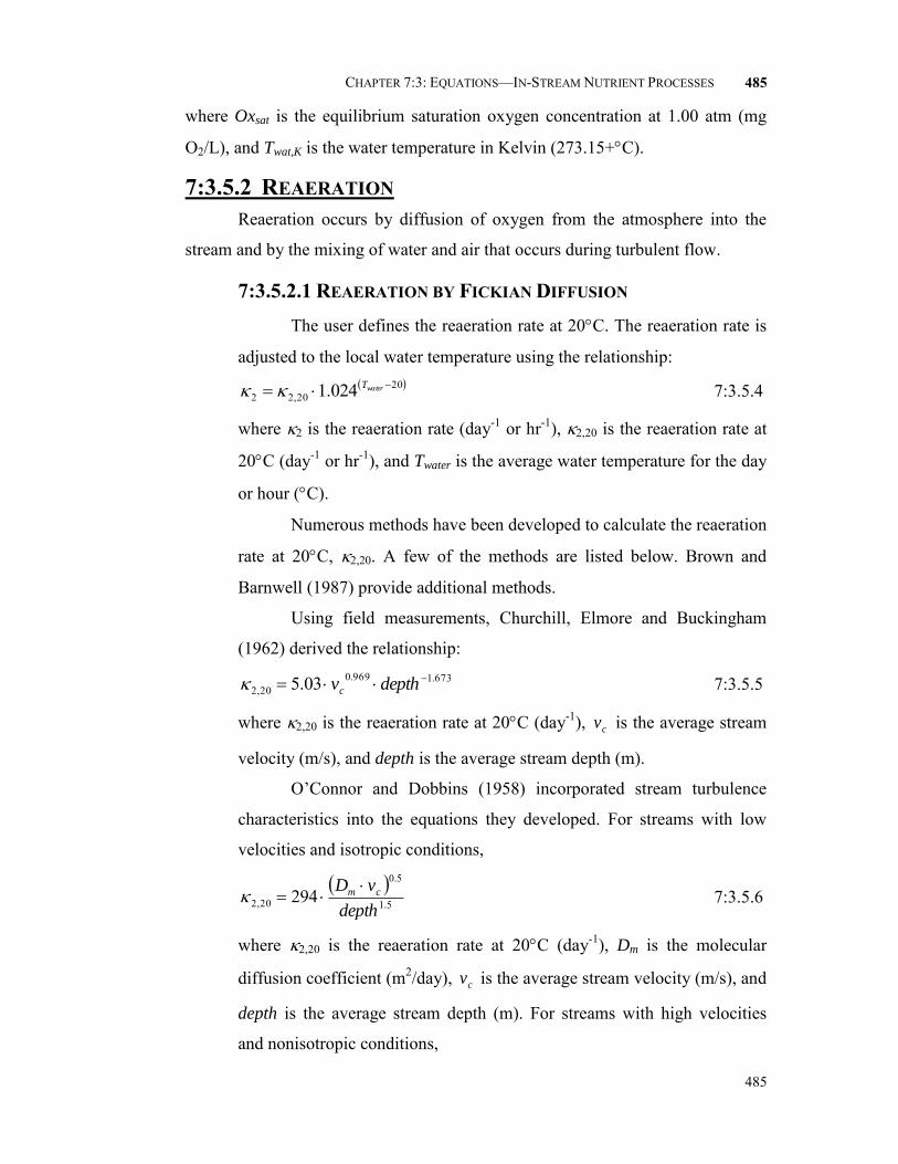
CHAPTER 7:3: EQUATIONS—IN-STREAM NUTRIENT PROCESSES
485
485
where Oxsat is the equilibrium saturation oxygen concentration at 1.00 atm (mg
O2/L), and Twat,K is the water temperature in Kelvin (273.15+C).
7:3.5.2 REAERATION
Reaeration occurs by diffusion of oxygen from the atmosphere into the
stream and by the mixing of water and air that occurs during turbulent flow.
7:3.5.2.1 REAERATION BY FICKIAN DIFFUSION The user defines the reaeration rate at 20C. The reaeration rate is
adjusted to the local water temperature using the relationship: 20
20,22 024.1 waterT 7:3.5.4
where 2 is the reaeration rate (day-1 or hr-1), 2,20 is the reaeration rate at
20C (day-1 or hr-1), and Twater is the average water temperature for the day
or hour (C).
Numerous methods have been developed to calculate the reaeration
rate at 20C, 2,20. A few of the methods are listed below. Brown and
Barnwell (1987) provide additional methods.
Using field measurements, Churchill, Elmore and Buckingham
(1962) derived the relationship: 673.1969.0
20,2 03.5 depthvc 7:3.5.5
where 2,20 is the reaeration rate at 20C (day-1), cv is the average stream
velocity (m/s), and depth is the average stream depth (m).
O’Connor and Dobbins (1958) incorporated stream turbulence
characteristics into the equations they developed. For streams with low
velocities and isotropic conditions,
5.1
5.0
20,2 294depth
vD cm 7:3.5.6
where 2,20 is the reaeration rate at 20C (day-1), Dm is the molecular
diffusion coefficient (m2/day), cv is the average stream velocity (m/s), and
depth is the average stream depth (m). For streams with high velocities
and nonisotropic conditions,

486 SWAT THEORETICAL DOCUMENTATION, VERSION 2009
486
25.1
25.05.0
20,2 2703depth
slpDm 7:3.5.7
where 2,20 is the reaeration rate at 20C (day-1), Dm is the molecular
diffusion coefficient (m2/day), slp is the slope of the streambed (m/m), and
depth is the average stream depth (m). The molecular diffusion coefficient
is calculated 20037.1177
waterT
mD 7:3.5.8
where Dm is the molecular diffusion coefficient (m2/day), and waterT is the
average water temperature (C).
Owens et al. (1964) developed an equation to determine the
reaeration rate for shallow, fast moving streams where the stream depth is
0.1 to 3.4 m and the velocity is 0.03 to 1.5 m/s.
85.1
67.0
20,2 34.5depth
vc 7:3.5.9
where 2,20 is the reaeration rate at 20C (day-1), cv is the average stream
velocity (m/s), and depth is the average stream depth (m).
7:3.5.2.2 REAERATION BY TURBULENT FLOW OVER A DAM Reareation will occur when water falls over a dam, weir, or other
structure in the stream. To simulate this form of reaeration, a “structure”
command line is added in the watershed configuration file (.fig) at every
point along the stream where flow over a structure occurs.
The amount of reaeration that occurs is a function of the oxygen
deficit above the structure and a reaeration coefficient:
reaDDDOx abastr
11 7:3.5.10
where Oxstr is the change in dissolved oxygen concentration (mg O2/L),
Da is the oxygen deficit above the structure (mg O2/L), Db is the oxygen
deficit below the structure (mg O2/L), and rea is the reaeration coefficient.
The oxygen deficit above the structure, Da, is calculated:

CHAPTER 7:3: EQUATIONS—IN-STREAM NUTRIENT PROCESSES
487
487
strsata OxOxD 7:3.5.11
where Oxsat is the equilibrium saturation oxygen concentration (mg O2/L),
and Oxstr is the dissolved oxygen concentration in the stream (mg O2/L).
Butts and Evans (1983) documents the following relationship that
can be used to estimate the reaeration coefficient:
waterfallfallba Thhcoefcoefrea 046.0111.0138.01 7:3.5.12
where rea is the reaeration coefficient, coefa is an empirical water quality
factor, coefb is an empirical dam aeration coefficient, hfall is the height
through which water falls (m), and waterT is the average water temperature
(C).
The empirical water quality factor is assigned a value based on the
condition of the stream:
coefa = 1.80 in clean water
coefa = 1.60 in slightly polluted water
coefa = 1.00 in moderately polluted water
coefa = 0.65 in grossly polluted water
The empirical dam aeration coefficient is assigned a value based
on the type of structure:
coefb = 0.70 to 0.90 for flat broad crested weir
coefb = 1.05 for sharp crested weir with straight slope face
coefb = 0.80 for sharp crested weir with vertical face
coefb = 0.05 for sluice gates with submerged discharge
Table 7:3-5: SWAT input variables used in in-stream oxygen calculations.
Variable name
Definition File
Name RK2 2,20: Reaeration rate at 20C (day-1) .swq AI3 3: Rate of oxygen production per unit algal photosynthesis (mg
O2/mg alg) .wwq
AI4 4: Rate of oxygen uptake per unit algal respiration (mg O2/mg alg) .wwq RHOQ a,20: Local algal respiration rate at 20C (day-1) .wwq RK1 1,20: CBOD deoxygenation rate at 20C (day-1) .swq RK4 4,20: Sediment oxygen demand rate at 20C (mg O2/(m2
day)) .swq AI5 5: Rate of oxygen uptake per unit NH4
+ oxidation (mg O2/mg N) .wwq AI6 6: Rate of oxygen uptake per unit NO2 oxidation (mg O2/mg N) .wwq AERATION_COEF rea: Reaeration coefficient .fig

488 SWAT THEORETICAL DOCUMENTATION, VERSION 2009
488
7:3.6 NOMENCLATURE CNH4 Concentration of ammonium in the reach (mg N/L) CNO3 Concentration of nitrate in the reach (mg N/L) CsolP Concentration of phosphorus in solution in the reach (mg P/L) Da Oxygen deficit above the structure (mg O2/L) Db Oxygen deficit below the structure (mg O2/L) Dm Molecular diffusion coefficient for oxygen (m2/day) FL Algal growth attenuation factor for light for the water column
FLz Algal growth attenuation factor for light at depth z
FN Algal growth limitation factor for nitrogen FP Algal growth limitation factor for phosphorus Hday Solar radiation reaching ground on current day of simulation (MJ m-2 d-1) Ihr Solar radiation reaching ground during specific hour on current day of simulation
(MJ m-2 h-1) Iphosyn,hr Photosynthetically-active solar radiation reaching ground during specific hour on
current day of simulation (MJ m-2 h-1) Iphosyn,z Photosynthetically-active light intensity at a depth z below the water surface
(MJ/m2-hr) hrphosynI , Daylight average photosynthetically-active light intensity (MJ/m2-hr)
KL Half-saturation coefficient for light (MJ/m2-hr) KN Michaelis-Menton half-saturation constant for nitrogen (mg N/L) KP Michaelis-Menton half-saturation constant for phosphorus (mg P/L) NH4str Ammonium concentration in the stream (mg N/L) NO2str Nitrite concentration in the stream (mg N/L) NO3str Nitrate concentration in the stream (mg N/L) Oxsat Saturation oxygen concentration (mg O2/L) Oxstr Dissolved oxygen concentration in the stream (mg O2/L) TDL Daylength (h) Twater Average daily or hourly water temperature (C) Twat,K Water temperature in Kelvin (273.15+C)
waterT Average water temperature (C) TT Travel time (day)
algae Algal biomass concentration (mg alg/L) cbod Carbonaceous biological oxygen demand concentration (mg CBOD/L) chla Chlorophyll a concentration (μg chla/L) coefa Empirical water quality factor coefb Empirical dam aeration coefficient depth Depth of water in the channel (m) fNH4 Preference factor for ammonia nitrogen
frDL Fraction of daylight hours
frNH4 Fraction of algal nitrogen uptake from ammonium pool, frphosyn Fraction of solar radiation that is photosynthetically active hfall Height through which water falls (m)

CHAPTER 7:3: EQUATIONS—IN-STREAM NUTRIENT PROCESSES
489
489
k Light extinction coefficient (m-1)
0,k Non-algal portion of the light extinction coefficient (m-1)
1,k Linear algal self shading coefficient (m-1 (μg-chla/L)-1)
2,k Nonlinear algal self shading coefficient (m-1 (μg-chla/L)-2/3) orgNstr Organic nitrogen concentration in the stream (mg N/L) orgPstr Organic phosphorus concentration in the stream (mg P/L) rea Reaeration coefficient slp Slope of the streambed (m/m)
cv Average stream velocity (m/s) z Depth from the water surface (m)
0 Ratio of chlorophyll a to algal biomass (μg chla/mg alg) 1 Fraction of algal biomass that is nitrogen (mg N/mg alg biomass), 2 Fraction of algal biomass that is phosphorus (mg P/mg alg biomass) 3 Rate of oxygen production per unit algal photosynthesis (mg O2/mg alg) 4 Rate of oxygen uptake per unit algal respiration (mg O2/mg alg) 5 Rate of oxygen uptake per unit NH4
+ oxidation (mg O2/mg N) 6 Rate of oxygen uptake per unit NO2 oxidation (mg O2/mg N) N,1 Rate constant for biological oxidation of ammonia nitrogen (day-1 or hr-1) N,1,20 Rate constant for biological oxidation of ammonia nitrogen at 20C (day-1 or hr-1) N,2 Rate constant for biological oxidation of nitrite to nitrate (day-1 or hr-1) N,2,20 Rate constant for biological oxidation of nitrite to nitrate at 20C (day-1 or hr-1) N,3 Rate constant for hydrolysis of organic nitrogen to ammonia nitrogen (day-1 or hr-1) N,3,20 Local rate constant for hydrolysis of organic nitrogen to NH4
+ at 20C (day-1 or hr-1)
P,4 Rate constant for mineralization of organic phosphorus (day-1 or hr-1) P,4,20 Local rate constant for organic phosphorus mineralization at 20C (day-1 or hr-1) algae Change in algal biomass concentration (mg alg/L) NH4str Change in ammonium concentration (mg N/L) NO2str Change in nitrite concentration (mg N/L) orgNstr Change in organic nitrogen concentration (mg N/L) orgPstr Change in organic phosphorus concentration (mg P/L) Oxstr Change in dissolved oxygen concentration (mg O2/L) solPstr Change in solution phosphorus concentration (mg P/L) 1 CBOD deoxygenation rate (day-1 or hr-1) 1,20 CBOD deoxygenation rate at 20C (day-1 or hr-1) 2 Reaeration rate for Fickian diffusion (day-1 or hr-1) 2,20 Reaeration rate at 20C (day-1 or hr-1) 3 Settling loss rate of CBOD (day-1 or hr-1) 3,20 Settling loss rate of CBOD at 20C (day-1 or hr-1) 4 Sediment oxygen demand rate (mg O2/(m2
day)) 4,20 Sediment oxygen demand rate at 20C (mg O2/(m2
day) or mg O2/(m2hr))
a Local respiration rate of algae (day-1 or hr-1)

490 SWAT THEORETICAL DOCUMENTATION, VERSION 2009
490
a,20 Local algal respiration rate at 20C (day-1 or hr-1) 1 Local settling rate for algae (m/day or m/hr) 1,20 Local algal settling rate at 20C (m/day or m/hr) 2 Benthos (sediment) source rate for soluble P (mg P/m2-day or mg P/m2-hr) 2,20 Benthos (sediment) source rate for soluble phosphorus at 20C (mg P/m2-day or mg
P/m2-hr) 3 Benthos (sediment) source rate for ammonium (mg N/m2-day or mg N/m2-hr) 3,20 Benthos (sediment) source rate for ammonium nitrogen at 20C (mg N/m2-day or
mg N/m2-hr) 4 Rate coefficient of organic nitrogen settling (day-1 or hr-1) 4,20 Local settling rate for organic nitrogen at 20C (day-1 or hr-1) 5 Rate coefficient for organic phosphorus settling (day-1 or hr-1) 5,20 Local settling rate for organic phosphorus at 20C (day-1 or hr-1) a Local specific growth rate of algae (day-1 or hr-1) a,20 Local specific algal growth rate at 20C (day-1 or hr-1) max Maximum specific algal growth rate (day-1 or hr-1)
7:3.7 REFERENCES
American Public Health Association. 1985. Standard methods for the examination
of water and wastewater, 16th edition. American Public Health
Association, Inc.
Azevedo, J., and P.R. Stout. 1974. Farm animal manures: An overview of their
role in the agricultural environment (Service Manual no. 44). University of
California, Agricultural Experiment Station Extension.
Bowie, G.L. W.B. Mills, D.B. Porcella, C.L. Campbell, J.R. Pagenkopt, G.L.
Rupp, K.M. Johnson, P.W.H. Chan, and S.A. Gherini. 1985. Rates,
constants, and kinetic formulations in surface water quality modeling, 2nd
ed. EPA/600/3-85/040, U.S. Environmental Protection Agency, Athens,
GA.
Brown, L.C. and T.O. Barnwell, Jr. 1987. The enhanced water quality models
QUAL2E and QUAL2E-UNCAS documentation and user manual. EPA
document EPA/600/3-87/007. USEPA, Athens, GA.
Butts, T.A. and R.L. Evans. 1983. Small stream channel dam aeration
characteristics. Journal, Environmental Engineering Division, ASAE
109:555-573.

CHAPTER 7:3: EQUATIONS—IN-STREAM NUTRIENT PROCESSES
491
491
Churchill, M.A., H.L. Elmore, and R.A. Buckingham. 1962. The prediction of
stream reaeration rates. International Journal of Air and Water Pollution.
6: 467-504.
Loehr, R.C. 1970. Drainage and pollution from beef cattle feedlots (Proceedings
paper No. 7726). Journal of the Sanitary Engineers Division, American
Society of Civil Engineers, 96 (SA6): 1295-1309.
O’Connor, D.J. and W.E. Dobbins. 1958. Mechanism of reaeration in natural
streams. Trans. ASCE. 123:641-684.
Owens, M. R.W. Edwards, and J.W. Gibbs. 1964. Some reaeration studies in
streams. International Journal of Air and Water Pollution 8:469-486.
Paine, M.D. 1973. Confined animals and public environment (Great Plains Beef
Cattle Feeding Handbook, GPE-7000/EC-72-246). Lincoln: University of
Nebraska, College of Agriculture, Cooperative Extension Service.

492 SWAT THEORETICAL DOCUMENTATION, VERSION 2009
492
493
SECTION 7 CHAPTER 4
EQUATIONS:
IN-STREAM PESTICIDE TRANSFORMATIONS
SWAT incorporates a simple mass balance developed by Chapra (1997) to
model the transformation and transport of pesticides in streams. The model
assumes a well-mixed layer of water overlying a sediment layer. Only one
pesticide can be routed through the stream network. The pesticide to be routed is
defined by the variable IRTPEST in the .bsn file.
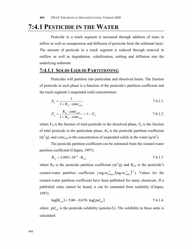
494 SWAT THEORETICAL DOCUMENTATION, VERSION 2009
494
7:4.1 PESTICIDE IN THE WATER
Pesticide in a reach segment is increased through addition of mass in
inflow as well as resuspension and diffusion of pesticide from the sediment layer.
The amount of pesticide in a reach segment is reduced through removal in
outflow as well as degradation, volatilization, settling and diffusion into the
underlying sediment.
7:4.1.1 SOLID-LIQUID PARTITIONING
Pesticides will partition into particulate and dissolved forms. The fraction
of pesticide in each phase is a function of the pesticide’s partition coefficient and
the reach segment’s suspended solid concentration:
sedd
dconcK
F
1
1 7:4.1.1
d
sedd
seddp F
concK
concKF
1
1 7:4.1.2
where Fd is the fraction of total pesticide in the dissolved phase, Fp is the fraction
of total pesticide in the particulate phase, Kd is the pesticide partition coefficient
(m3/g), and concsed is the concentration of suspended solids in the water (g/m3).
The pesticide partition coefficient can be estimated from the octanol-water
partition coefficient (Chapra, 1997):
owd KK 810085.3 7:4.1.3
where Kd is the pesticide partition coefficient (m3/g) and Kow is the pesticide’s
octanol-water partition coefficient ( 13water
3octanol m mg m mg ). Values for the
octanol-water partition coefficient have been published for many chemicals. If a
published value cannot be found, it can be estimated from solubility (Chapra,
1997):
solow tpsK log670.000.5log 7:4.1.4
where soltps is the pesticide solubility (μmoles/L). The solubility in these units is
calculated:

CHAPTER 7:4: EQUATIONS—IN-STREAM PESTICIDE TRANSFORMATIONS
495
495
310MW
psttps sol
sol 7:4.1.5
where soltps is the pesticide solubility (μmoles/L), pstsol is the pesticide solubility
(mg/L) and MW is the molecular weight (g/mole).
7:4.1.2 DEGRADATION Pesticides in both the particulate and dissolved forms are subject to
degradation. The amount of pesticide that is removed from the water via
degradation is:
TTpstkpst rchwtraqpdeg,wtr , 7:4.1.6
where pstdeg,wtr is the amount of pesticide removed from the water via degradation
(mg pst), kp,aq is the rate constant for degradation or removal of pesticide in the
water (1/day), pstrchwtr is the amount of pesticide in the water at the beginning of
the day (mg pst), and TT is the flow travel time (days). The rate constant is related
to the aqueous half-life:
aq
aqpt
k,2/1
,693.0
7:4.1.7
where kp,aq is the rate constant for degradation or removal of pesticide in the water
(1/day), and t1/2,aq is the aqueous half-life for the pesticide (days).
7:4.1.3 VOLATILIZATION Pesticide in the dissolved phase is available for volatilization. The amount
of pesticide removed from the water via volatilization is:
TTpstFdepth
vpst rchwtrd
vwtrvol , 7:4.1.8
where pstvol,wtr is the amount of pesticide removed via volatilization (mg pst), vv is
the volatilization mass-transfer coefficient (m/day), depth is the flow depth (m),
Fd is the fraction of total pesticide in the dissolved phase, pstrchwtr is the amount of
pesticide in the water (mg pst), and TT is the flow travel time (days).
The volatilization mass-transfer coefficient can be calculated based on
Whitman’s two-film or two-resistance theory (Whitman, 1923; Lewis and
Whitman, 1924 as described in Chapra, 1997). While the main body of the gas
and liquid phases are assumed to be well-mixed and homogenous, the two-film
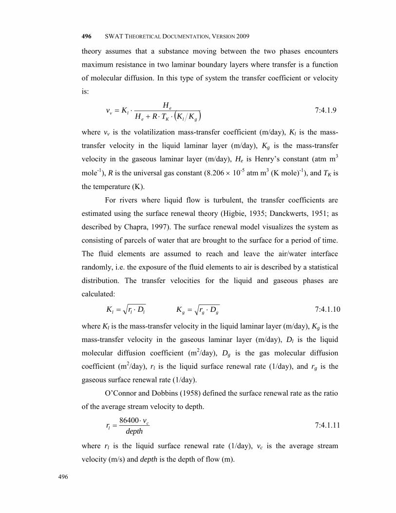
496 SWAT THEORETICAL DOCUMENTATION, VERSION 2009
496
theory assumes that a substance moving between the two phases encounters
maximum resistance in two laminar boundary layers where transfer is a function
of molecular diffusion. In this type of system the transfer coefficient or velocity
is:
glKe
elv
KKTRH
HKv
7:4.1.9
where vv is the volatilization mass-transfer coefficient (m/day), Kl is the mass-
transfer velocity in the liquid laminar layer (m/day), Kg is the mass-transfer
velocity in the gaseous laminar layer (m/day), He is Henry’s constant (atm m3
mole-1), R is the universal gas constant (8.206 10-5 atm m3 (K mole)-1), and TK is
the temperature (K).
For rivers where liquid flow is turbulent, the transfer coefficients are
estimated using the surface renewal theory (Higbie, 1935; Danckwerts, 1951; as
described by Chapra, 1997). The surface renewal model visualizes the system as
consisting of parcels of water that are brought to the surface for a period of time.
The fluid elements are assumed to reach and leave the air/water interface
randomly, i.e. the exposure of the fluid elements to air is described by a statistical
distribution. The transfer velocities for the liquid and gaseous phases are
calculated:
lll DrK ggg DrK 7:4.1.10
where Kl is the mass-transfer velocity in the liquid laminar layer (m/day), Kg is the
mass-transfer velocity in the gaseous laminar layer (m/day), Dl is the liquid
molecular diffusion coefficient (m2/day), Dg is the gas molecular diffusion
coefficient (m2/day), rl is the liquid surface renewal rate (1/day), and rg is the
gaseous surface renewal rate (1/day).
O’Connor and Dobbins (1958) defined the surface renewal rate as the ratio
of the average stream velocity to depth.
depth
vr cl
86400 7:4.1.11
where rl is the liquid surface renewal rate (1/day), vc is the average stream
velocity (m/s) and depth is the depth of flow (m).
CHAPTER 7:4: EQUATIONS—IN-STREAM PESTICIDE TRANSFORMATIONS
497
497
7:4.1.4 SETTLING Pesticide in the particulate phase may be removed from the water layer by
settling. Settling transfers pesticide from the water to the sediment layer. The
amount of pesticide that is removed from the water via settling is:
TTpstFdepth
vpst rchwtrp
swtrstl , 7:4.1.12
where pststl,wtr is the amount of pesticide removed from the water due to settling
(mg pst), vs is the settling velocity (m/day), depth is the flow depth (m), Fp is the
fraction of total pesticide in the particulate phase, pstrchwtr is the amount of
pesticide in the water (mg pst), and TT is the flow travel time (days).
7:4.1.5 OUTFLOW Pesticide is removed from the reach segment in outflow. The amount of
dissolved and particulate pesticide removed from the reach segment in outflow is:
V
pstFQpst rchwtrd
osol
, 7:4.1.13
V
pstFQpst
rchwtrp
osorb
, 7:4.1.14
where pstsol,o is the amount of dissolved pesticide removed via outflow (mg pst),
pstsorb,o is the amount of particulate pesticide removed via outflow (mg pst), Q is
the rate of outflow from the reach segment (m3 H2O/day), Fd is the fraction of
total pesticide in the dissolved phase, Fp is the fraction of total pesticide in the
particulate phase, pstrchwtr is the amount of pesticide in the water (mg pst), and V
is the volume of water in the reach segment (m3 H2O).
Table 7:4-1: SWAT input variables that pesticide partitioning. Variable
Name
Definition Input File
CHPST_KOC Kd: Pesticide partition coefficient (m3/g) .swq CHPST_REA kp,aq: Rate constant for degradation or removal of pesticide in the
water (1/day) .swq
CHPST_VOL vv: Volatilization mass-transfer coefficient (m/day) .swq CHPST_STL vs: Pesticide settling velocity (m/day) .swq

498 SWAT THEORETICAL DOCUMENTATION, VERSION 2009
498
7:4.2 PESTICIDE IN THE SEDIMENT
Pesticide in the sediment layer underlying a reach segment is increased
through addition of mass by settling and diffusion from the water. The amount of
pesticide in the sediment layer is reduced through removal by degradation,
resuspension, diffusion into the overlying water, and burial.
7:4.2.1 SOLID-LIQUID PARTITIONING As in the water layer, pesticides in the sediment layer will partition into
particulate and dissolved forms. Calculation of the solid-liquid partitioning in the
sediment layer requires a suspended solid concentration. The “concentration” of
solid particles in the sediment layer is defined as:
tot
sedsed
V
Mconc * 7:4.2.1
where *sedconc is the “concentration” of solid particles in the sediment layer
(g/m3), Msed is the mass of solid particles in the sediment layer (g) and Vtot is the
total volume of the sediment layer (m3).
Mass and volume are also used to define the porosity and density of the
sediment layer. In the sediment layer, porosity is the fraction of the total volume
in the liquid phase:
tot
wtr
V
V 7:4.2.2
where is the porosity, Vwtr is the volume of water in the sediment layer (m3) and
Vtot is the total volume of the sediment layer (m3). The fraction of the volume in
the solid phase can then be defined as:
tot
sed
V
V1 7:4.2.3
where is the porosity, Vsed is the volume of solids in the sediment layer (m3) and
Vtot is the total volume of the sediment layer (m3).
The density of sediment particles is defined as:
sed
seds
V
M 7:4.2.4

CHAPTER 7:4: EQUATIONS—IN-STREAM PESTICIDE TRANSFORMATIONS
499
499
where s is the particle density (g/m3), Msed is the mass of solid particles in the
sediment layer (g), and Vsed is the volume of solids in the sediment layer (m3).
Solving equation 7:4.2.3 for Vtot and equation 7:4.2.4 for Msed and
substituting into equation 7:4.2.1 yields:
ssedconc 1* 7:4.2.5
where *sedconc is the “concentration” of solid particles in the sediment layer
(g/m3), is the porosity, and s is the particle density (g/m3).
Assuming = 0.5 and s = 2.6 106 g/m3, the “concentration” of solid
particles in the sediment layer is 1.3 106 g/m3.
The fraction of pesticide in each phase is then calculated:
ds
seddK
F
1
1, 7:4.2.6
seddsedp FF ,, 1 7:4.2.7
where Fd,sed is the fraction of total sediment pesticide in the dissolved phase, Fp,sed
is the fraction of total sediment pesticide in the particulate phase, is the porosity,
s is the particle density (g/m3), and Kd is the pesticide partition coefficient (m3/g).
The pesticide partition coefficient used for the water layer is also used for the
sediment layer.
7:4.2.2 DEGRADATION Pesticides in both the particulate and dissolved forms are subject to
degradation. The amount of pesticide that is removed from the sediment via
degradation is:
rchsedsedpdeg,sed pstkpst , 7:4.2.8
where pstdeg,sed is the amount of pesticide removed from the sediment via
degradation (mg pst), kp,sed is the rate constant for degradation or removal of
pesticide in the sediment (1/day), and pstrchsed is the amount of pesticide in the
sediment (mg pst). The rate constant is related to the sediment half-life:
sed
sedpt
k,2/1
,693.0
7:4.2.9
500 SWAT THEORETICAL DOCUMENTATION, VERSION 2009
500
where kp,sed is the rate constant for degradation or removal of pesticide in the
sediment (1/day), and t1/2,sed is the sediment half-life for the pesticide (days).
7:4.2.3 RESUSPENSION Pesticide in the sediment layer is available for resuspension. The amount
of pesticide that is removed from the sediment via resuspension is:
TTpstdepth
vpst rchsed
rwtrrsp , 7:4.2.10
where pstrsp,wtr is the amount of pesticide removed via resuspension (mg pst), vr is
the resuspension velocity (m/day), depth is the flow depth (m), pstrchsed is the
amount of pesticide in the sediment (mg pst), and TT is the flow travel time
(days). Pesticide removed from the sediment layer by resuspension is added to the
water layer.
7:4.2.4 DIFFUSION Pesticide in the dissolved phase is available for diffusion. Diffusion
transfers pesticide between the water and sediment layers. The direction of
movement is controlled by the pesticide concentration. Pesticide will move from
areas of high concentration to areas of low concentration. The amount of pesticide
that is transferred between the water and sediment by diffusion is:
TTpstFpstFdepth
vpst rchwtrdrchsedsedd
ddif , 7:4.2.11
where pstdif is the amount of pesticide transferred between the water and sediment
by diffusion (mg pst), vd is the rate of diffusion or mixing velocity (m/day), depth
is the flow depth (m), Fd,sed is the fraction of total sediment pesticide in the
dissolved phase, pstrchsed is the amount of pesticide in the sediment (mg pst), Fd is
the fraction of total water layer pesticide in the dissolved phase, pstrchwtr is the
amount of pesticide in the water (mg pst), and TT is the flow duration (days). If
rchwtrdrchsedsedd pstFpstF , , pstdif is transferred from the sediment to the water
layer. If, rchwtrdrchsedsedd pstFpstF , , pstdif is transferred from the water to the
sediment layer.

CHAPTER 7:4: EQUATIONS—IN-STREAM PESTICIDE TRANSFORMATIONS
501
501
The diffusive mixing velocity, vd, can be estimated from the empirically
derived formula (Chapra, 1997):
3/2
36535.69 MWvd 7:4.2.12
where vd is the rate of diffusion or mixing velocity (m/day), is the sediment
porosity, and MW is the molecular weight of the pesticide compound.
7:4.2.5 BURIAL Pesticide in the sediment layer may be lost by burial. The amount of
pesticide that is removed from the sediment via burial is:
rchsed
sed
bbur pst
D
vpst 7:4.2.13
where pstbur is the amount of pesticide removed via burial (mg pst), vb is the burial
velocity (m/day), Dsed is the depth of the active sediment layer (m), and pstrchsed is
the amount of pesticide in the sediment (mg pst).
Table 7:4-2: SWAT input variables related to pesticide in the sediment. Variable Name
Definition Input File
CHPST_KOC Kd: Pesticide partition coefficient (m3/g) .swq SEDPST_REA kp,sed: Rate constant for degradation or removal of pesticide in the
sediment (1/day) .swq
CHPST_RSP vr: Resuspension velocity (m/day) .swq SEDPST_ACT Dsed: Depth of the active sediment layer (m) .swq CHPST_MIX vd: Rate of diffusion or mixing velocity (m/day) .swq SEDPST_BRY vb: Pesticide burial velocity (m/day) .swq
7:4.3 MASS BALANCE The processes described above can be combined into mass balance
equations for the well-mixed reach segment and the well-mixed sediment layer:
wtrvolwtrdegosorbosolinrchwtr pstpstpstpstpstpst ,,,,
difwtrrspwtrstl pstpstpst ,, 7:4.3.1
difburwtrrspwtrstldeg,sedrchsed pstpstpstpstpstpst ,, 7:4.3.2
where pstrchwtr is the change in pesticide mass in the water layer (mg pst),
pstrchsed is the change in pesticide mass in the sediment layer (mg pst), pstin is the

502 SWAT THEORETICAL DOCUMENTATION, VERSION 2009
502
pesticide added to the reach segment via inflow (mg pst), pstsol,o is the amount of
dissolved pesticide removed via outflow (mg pst), pstsorb,o is the amount of
particulate pesticide removed via outflow (mg pst), pstdeg,wtr is the amount of
pesticide removed from the water via degradation (mg pst), pstvol,wtr is the amount
of pesticide removed via volatilization (mg pst), pststl,wtr is the amount of pesticide
removed from the water due to settling (mg pst), pstrsp,wtr is the amount of
pesticide removed via resuspension (mg pst), pstdif is the amount of pesticide
transferred between the water and sediment by diffusion (mg pst), pstdeg,sed is the
amount of pesticide removed from the sediment via degradation (mg pst), pstbur is
the amount of pesticide removed via burial (mg pst).
7:3.4 NOMENCLATURE Dg Gas molecular diffusion coefficient (m2/day) Dl Liquid molecular diffusion coefficient (m2/day) Dsed Depth of the active sediment layer (m) Fd Fraction of total pesticide in the dissolved phase Fd,sed Fraction of total sediment pesticide in the dissolved phase Fp Fraction of total pesticide in the particulate phase Fp,sed Fraction of total sediment pesticide in the particulate phase
He Henry’s constant (atm m3 mole-1) Kd Pesticide partition coefficient (m3/g) Kg Mass-transfer velocity in the gaseous laminar layer (m/day) Kl Mass-transfer velocity in the liquid laminar layer (m/day) Msed Mass of solid phase in the sediment layer (g) MW Molecular weight of the pesticide compound
Q Rate of outflow from the reach segment (m3 H2O/day) R Universal gas constant (8.206 10-5 atm m3 (K mole)-1) Vsed Volume of solids in the sediment layer (m3) Vtot Total volume of the sediment layer (m3) Vwtr Volume of water in the sediment layer (m3) concsed Concentration of suspended solids in the water (g/m3)
*sedconc “Concentration” of solid particles in the sediment layer (g/m3)
depth Depth of flow (m) kp,aq Rate constant for degradation or removal of pesticide in the water (1/day) kp,sed Rate constant for degradation or removal of pesticide in the sediment (1/day) pstbur Amount of pesticide removed via burial (mg pst) pstdeg,sed Amount of pesticide removed from the sediment via degradation (mg pst)
CHAPTER 7:4: EQUATIONS—IN-STREAM PESTICIDE TRANSFORMATIONS
503
503
pstdeg,wtr Amount of pesticide removed from the water via degradation (mg pst) pstdif Amount of pesticide transferred between the water and sediment by diffusion (mg
pst) pstrchsed Amount of pesticide in the sediment (mg pst) pstrchwtr Amount of pesticide in the water (mg pst) pstrsp,wtr Amount of pesticide removed from sediment via resuspension (mg pst) pstsol,o Amount of dissolved pesticide removed via outflow (mg pst) pstsorb,o Amount of particulate pesticide removed via outflow (mg pst) pststl,wtr Amount of pesticide removed from the water due to settling (mg pst) pstvol,wtr Amount of pesticide removed via volatilization (mg pst) rg Gaseous surface renewal rate (1/day) rl Liquid surface renewal rate (1/day) t1/2,aq Aqueous half-life for the pesticide (days) t1/2,sed Sediment half-life for the pesticide (days) vb Pesticide burial velocity (m/day) vc Average stream velocity (m/s) vd Rate of diffusion or mixing velocity (m/day) vr Resuspension velocity (m/day) vs Settling velocity (m/day) vv Volatilization mass-transfer coefficient (m/day) pstrchwtr Change in pesticide mass in the water layer (mg pst) pstrchsed Change in pesticide mass in the sediment layer (mg pst) Porosity s Particle density (g/m3)
7:4.5 REFERENCES
Chapra, S.C. 1997. Surface water-quality modeling. WCB/McGraw-Hill, Boston, MA.
Danckwerts, P.V. 1951. Significance of liquid-film coefficients in gas absorption. Ind. Eng. Chem. 43:1460-1467.
Higbie, R. 1935. The rate of adsorption of a pure gas into a still liquid during short periods of exposure. Trans. Amer. Inst. Chem. Engin. 31:365-389.
Lewis, W.K. and W.G. Whitman. 1924. Principles of gas absorption. Ind. Eng. Chem. 16:1215-1220.
O'Connor, D.J. and Dobbins, W.E. 1958. Mechanisms of reaeration in natural streams. Trans ASAE 123: 641-666.
Whitman, W.G. 1923. The two-film theory of gas adsorption. Chem. Metallurg. Eng. 29:146-148.

504 SWAT THEORETICAL DOCUMENTATION, VERSION 2009
504

505
SECTION 7 CHAPTER 5
EQUATIONS:
BACTERIA ROUTING
SWAT calculates loading of pathogens and indicator bacteria for
pathogens from land areas in the watershed. In the stream, bacteria die-off is the
only process modeled.

506 SWAT THEORETICAL DOCUMENTATION, VERSION 2009
506
7:5.1 BACTERIA DECAY A first order decay function is used to calculate changes in bacteria
concentrations (Bowie et al., 1985).
dielprchilprchilprch bactbact ,1,, exp 7:5.1.1
dieprchiprchiprch bactbact ,1,, exp 7:5.1.2
where bactlprch,i is the amount of less persistent bacteria present in the reach on
day i (#cfu/100mL), bactlprch,i-1 is the amount of less persistent bacteria present in
the reach on day i - 1 (#cfu/100mL), μlprch,die is the rate constant for die-off of less
persistent bacteria in streams (1/day), bactprch,i is the amount of persistent bacteria
present in the reach on day i (#cfu/100mL), bactprch,i-1 is the amount of persistent
bacteria present in the reach on day i - 1 (#cfu/100mL), and μprch,die, is the rate
constant for die-off of persistent bacteria in streams (1/day).
The die-off rate constants are adjusted for temperature using the equations: 20
20,,,
waterT
bactdielprchdielprch 7:5.1.3
2020,,,
waterT
bactdieprchdieprch 7:5.1.4
where μlprch,die, is the rate constant for die-off of less persistent bacteria in streams
(1/day), μprch,die is the rate constant for die-off of persistent bacteria in streams
(1/day), μlprch,die,20 is the rate constant for die-off of less persistent bacteria in
streams at 20C (1/day), μprch,die,20 is the rate constant for die-off of persistent
bacteria in streams at 20C (1/day), θbact is the temperature adjustment factor for
bacteria die-off/re-growth, and Twater is the water temperature (C).
Table 7:5-1: SWAT input variables that pertain to bacteria die-off in the stream.
Variable Name
Definition Input File
WDPRCH μprch,die,20: Die-off factor for persistent bacteria in streams at 20C (1/day)
.bsn
WDLPRCH μlprch,die,20: Die-off factor for less persistent bacteria in streams at 20C (1/day)
.bsn
THBACT θbact: Temperature adjustment factor for bacteria die-off/growth .bsn
CHAPTER 7:5: EQUATIONS—BACTERIA ROUTING
507
507
7:5.2 BACTERIA SEDIMENT
In sediment channel routing, the maximum concentration of sediment that can be
transported by the water, concsed,ch,mx, (ton/m3 or kg/L) is compared to the
concentration of sediment in the reach at the beginning of the time step,
concsed,ch,i (Neitsch et al., 2005).
If concsed,ch,i < concsed,ch,mx, resuspension is the dominant process in the
reach segment and the net amount of sediment reentrained is calculated:
chchchichsedmxchseddeg CKVconcconcsed ,,,, 7:5.2.1
where seddeg is the amount of sediment reentrained in the reach segment (metric
tons), concsed,ch,mx is the maximum concentration of sediment that can be
transported by the water (ton sediment/m3 H2O or kg sediment/L H2O),
concsed,ch,i is the initial sediment concentration in the reach (ton sediment/m3 H2O
or kg sediment/L H2O), Vch is the volume of water in the reach segment (m3
H2O), Kch is the channel erodibility factor (cm/hr/Pa), and Cch is the channel
cover factor. When sediment resuspends, both bacteria in sediment solution and
on sediment particles are released, and the net amount of bacteria released from
streambed is calculated:
sedbactdegdeg concsedbact , 7:5.2.2
where bactdeg is the amount of bacteria released from streambed in the reach
segment (# cfu), seddeg is the amount of sediment reentrained in the reach
segment (metric tons), and concbact,sed is the concentration of bacteria in
streambed in the reach segment (# cfu/ton sediment). Bacteria concentration in
streambed is calculated by the empirical regression equation, logarithmic sine
function of the days of year:
43
21, 366sinlog bsc
bscdaybscbscconc sedbac
7:5.2.3
where concbac,sed is the concentration of bacteria in streambed (# cfu/ton
sediment), day is the days of year, and bsc1 through bsc4 are the regression
coefficients in streambed bacteria concentration equation.
508 SWAT THEORETICAL DOCUMENTATION, VERSION 2009
508
If concsed,ch,i > concsed,ch,mx, deposition is the dominant process in the
reach segment and the net amount of sediment deposited is calculated:
chmxchsedichseddep Vconcconcsed ,,,, 7:5.2.4
where seddep is the amount of sediment deposited in the reach segment (metric
tons), concsed,ch,i is the initial sediment concentration in the reach (ton
sediment/m3 H2O or kg sediment/L H2O), concsed,ch,mx is the maximum
concentration of sediment that can be transported by the water (ton sediment/m3
H2O or kg sediment/L H2O), and Vch is the volume of water in the reach segment
(m3 H2O). When suspended sediment deposits, bacteria on settling sediment
particles are deposited, and the net amount of bacteria settled from stream water
is calculated (Bai and Lung, 2005):
chichsedpch
depp
ichdepVconcKV
sedKbactbact
,,, 7:5.2.5
where bactdep is the amount of bacteria settled from stream water in the reach
segment (# cfu), bactch,i is the amount of bacteria in the stream water in the reach
segment at the beginning of the time period (# cfu), Kp is the linear partitioning
coefficient of bacteria between the suspended sediment and water (m3 H2O/ton
sediment or L H2O/kg sediment), seddep is the amount of sediment deposited in
the reach segment (metric tons), Vch is the volume of water in the reach segment
(m3 H2O), and concsed,ch,i is the initial sediment concentration in the reach (ton
sediment/m3 H2O or kg sediment/L H2O). The linear partitioning coefficient is
calculated from the empirical regression equation (Pachepsky et al., 2006): 98.16.110 clayK p 7:5.2.6
where Kp is the linear partitioning coefficient of bacteria onto the suspended
sediment (m3 H2O/ton sediment or L H2O/kg sediment) and clay is the
percentage of clay in suspended sediment in stream water in the reach segment
(%). clay normally varies between 2 and 50%.
Once the amount of bacteria released and settled has been calculated, the
final amount of sediment in the reach is determined:
depdegichch bactbactbactbact , 7:5.2.7

CHAPTER 7:5: EQUATIONS—BACTERIA ROUTING
509
509
where bactch is the amount of bacteria in the stream water in the reach segment
(# cfu), bactch,i is the amount of bacteria in the stream water in the reach segment
at the beginning of the time period (# cfu), bactdeg is the amount of bacteria
released from streambed in the reach segment (# cfu), and bactdep is the amount
of bacteria settled from stream water in the reach segment (# cfu).
The final bacteria concentration in the reach is calculated:
4, 10
ch
chchbact
V
bactconc 7:5.2.8
where concbact,ch is the concentration of bacteria in the stream water in the reach
segment (# cfu/100 mL), bactch is the amount of bacteria in the stream water in
the reach segment (# cfu), and Vch is the volume of water in the reach segment
(m3 H2O).
7:5.3 NOMENCLATURE
Twater Average daily water temperature (C) bactlprch Amount of less persistent bacteria present in the reach (#cfu/100mL) bactprch Amount of persistent bacteria present in the reach (#cfu/100mL)
θbact Temperature adjustment factor for bacteria die-off/re-growth μlprch,die Rate constant for die-off of less persistent bacteria in streams (1/day)
μlprch,die,20 Rate constant for die-off of less persistent bacteria in streams at 20C (1/day) μprch,die Rate constant for die-off of persistent bacteria in streams (1/day) μprch,die,20 Rate constant for die-off of persistent bacteria in streams at 20C (1/day)
7:5.4 REFERENCES Bai, S.; Lung, W.S., 2005. Modeling sediment impact on the transport of fecal
bacteria. Water Research, 39(20): 5232-5240.
Bowie, G.W., W. Mills, D. Porcella, C. Campbell, J. Pagenkopf, G. Rupp, K. Johnson, P.
Chan, S. Gherini, and C. Chamberlin. 1985. Rates, constants and kinetics
formulations in surface water quality modeling. 2nd ed. USEPA/600/3-85-040.
Byappanahalli, M.; Fowler, M.; Shively, D.; Whitman, R., 2003. Ubiquity and
persistence of Escherichia coli in a midwestern coastal stream. Applied and
Environmental Microbiology, 69(8): 4549-4555.

510 SWAT THEORETICAL DOCUMENTATION, VERSION 2009
510
Cinotto, P.J., 2005. Occurrence of fecal-indicator bacteria and protocols for identification
of fecal-contamination sources in selected reaches of the West Branch Brandywine
Creek, Chester County, Pennsylvania: U.S. Geological Survey Scientific
Investigations Report 2005-5039, pp 91.
Davies, C.M.; Long, J.A.H.; Donald, M.; Ashbolt, N.J., 1995. Survival of fecal
microorganisms in marine and fresh-water sediments. Applied and Environmental
Microbiology, 61(5): 1888-1896.
Gannon, J.J.; Busse, M.K.; Schillinger, J.E., 1983. Fecal coliform disappearance in a
river impoundment. Water Research, 17(11): 1595-1601.
Giddings, E.M.; Oblinger, C.J., 2004. Fecal-indicator bacteria in the Newfound Creek
watershed, western North Carolina, during a high and low streamflow condition,
2003: U.S. Geological Survey Scientific Investigations Report 2004–5257,
accessed January 18, 2005, at http://pubs.water.usgs.gov/sir2004-5257.
Muirhead, R.W.; Davies-Colley, R.J.; Donnison, A.M.; Nagels, J.W., 2004. Faecal
bacteria yields in artificial flood events: quantifying in-stream stores. Water
Research, 38: 1215-1224.
Neitsch, S.L.; Arnold, J.G.; Kiniry, J.R.; Williams, J.R., 2005. Soil and Water
Assessment Tool Theoretical Documentation (Version 2005).
Pachepsky, Y.A.; Sadeghi, A.M.; Bradford, S.A.; Shelton, D.R.; Guber, A.K.; Dao, T.,
2006. Transport and fate of manure-borne pathogens: Modeling perspective.
Agricultural Water Management, 86: 81-92.

CHAPTER 7:5: EQUATIONS—BACTERIA ROUTING
511
511

512
SECTION 7 CHAPTER 6
EQUATIONS:
HEAVY METAL ROUTING
Heavy metals are pollutants that are increasingly under scrutiny. Most
heavy metals can exist in a number of different valence states and the solubility of
a heavy metal is often dependent on the valence state it is in. The complexity of
the processes affecting heavy metal solubility make modeling these processes
directly unrealistic. At this time, SWAT allows heavy metal loadings to be added
to the stream network in point source loading inputs. SWAT currently routes the
heavy metals through the channel network, but includes no algorithms to model
in-stream processes. Simple mass balance equations are used to determine the
movement of heavy metals through the river network.

CHAPTER 7:4: EQUATIONS—IN-STREAM PESTICIDE TRANSFORMATIONS
513
513

WATER BODIES
Impoundment structures modify the movement
of water in the channel network by lowering the peak
flow and volume of flood discharges. Because
impoundments slow down the flow of water, sediment
will fall from suspension, removing nutrient and
chemicals adsorbed to the soil particles.

514
SECTION 8 CHAPTER 1
EQUATIONS:
IMPOUNDMENT WATER ROUTING
Impoundments play an important role in water supply and flood control.
SWAT models four types of water bodies: ponds, wetlands, depressions/potholes,
and reservoirs. Ponds, wetlands, and depressions/potholes are located within a
subbasin off the main channel. Water flowing into these water bodies must
originate from the subbasin in which the water body is located. Reservoirs are
located on the main channel network. They receive water from all subbasins
upstream of the water body.

CHAPTER 8:1: EQUATIONS—IMPOUNDMENT WATER ROUTING
515
515
8:1.1 RESERVOIRS A reservoir is an impoundment located on the main channel network of a
watershed. No distinction is made between naturally-occurring and man-made
structures. The features of an impoundment are shown in Figure 8:1.1.
Figure 8:1.1: Components of a reservoir with flood water detention features (After Ward and Elliot, 1995).
The water balance for a reservoir is:
seepevappcpflowoutflowinstored VVVVVVV 8:1.1.1
where V is the volume of water in the impoundment at the end of the day (m3
H2O), Vstored is the volume of water stored in the water body at the beginning of
the day (m3 H2O), Vflowin is the volume of water entering the water body during the
day (m3 H2O), Vflowout is the volume of water flowing out of the water body during
the day (m3 H2O), Vpcp is the volume of precipitation falling on the water body
during the day (m3 H2O), Vevap is the volume of water removed from the water
body by evaporation during the day (m3 H2O), and Vseep is the volume of water
lost from the water body by seepage (m3 H2O).
516 SWAT THEORETICAL DOCUMENTATION, VERSION 2009
516
8:1.1.1 SURFACE AREA The surface area of the reservoir is needed to calculate the amount of
precipitation falling on the water body as well as the amount of evaporation and
seepage. Surface area varies with change in the volume of water stored in the
reservoir. The surface area is updated daily using the equation:
expsa
sa VSA 8:1.1.2
where SA is the surface area of the water body (ha), sa is a coefficient, V is the
volume of water in the impoundment (m3 H2O), and expsa is an exponent.
The coefficient, sa, and exponent, expsa, are calculated by solving
equation 8:1.1.2 using two known points. The two known points are surface area
and volume information provided for the principal and emergency spillways.
prem
prem
VV
SASAexpsa
1010
1010
loglogloglog
8:1.1.3
expsa
em
emsa
V
SA
8:1.1.4
where SAem is the surface area of the reservoir when filled to the emergency
spillway (ha), SApr is the surface area of the reservoir when filled to the principal
spillway (ha), Vem is the volume of water held in the reservoir when filled to the
emergency spillway (m3 H2O), and Vpr is the volume of water held in the reservoir
when filled to the principal spillway (m3 H2O).
8:1.1.2 PRECIPITATION The volume of precipitation falling on the reservoir during a given day is
calculated:
SARV daypcp 10 8:1.1.5
where Vpcp is the volume of water added to the water body by precipitation during
the day (m3 H2O), Rday is the amount of precipitation falling on a given day (mm
H2O), and SA is the surface area of the water body (ha).
CHAPTER 8:1: EQUATIONS—IMPOUNDMENT WATER ROUTING
517
517
8:1.1.3 EVAPORATION The volume of water lost to evaporation on a given day is calculated:
SAEV oevap 10 8:1.1.6
where Vevap is the volume of water removed from the water body by evaporation
during the day (m3 H2O), is an evaporation coefficient (0.6), Eo is the potential
evapotranspiration for a given day (mm H2O), and SA is the surface area of the
water body (ha).
8:1.1.4 SEEPAGE The volume of water lost by seepage through the bottom of the reservoir
on a given day is calculated:
SAKV satseep 240 8:1.1.7
where Vseep is the volume of water lost from the water body by seepage (m3 H2O),
Ksat is the effective saturated hydraulic conductivity of the reservoir bottom
(mm/hr), and SA is the surface area of the water body (ha).
8:1.1.5 OUTFLOW The volume of outflow may be calculated using one of four different
methods: measured daily outflow, measured monthly outflow, average annual
release rate for uncontrolled reservoir, controlled outflow with target release.
8:1.1.5.1 MEASURED DAILY OUTFLOW When measured daily outflow (IRESCO = 3) is chosen as the
method to calculate reservoir outflow, the user must provide a file with the
outflow rate for every day the reservoir is simulated in the watershed. The
volume of outflow from the reservoir is then calculated:
outflowout qV 86400 8:1.1.8
where Vflowout is the volume of water flowing out of the water body during
the day (m3 H2O), and qout is the outflow rate (m3/s).

518 SWAT THEORETICAL DOCUMENTATION, VERSION 2009
518
8:1.1.5.2 MEASURED MONTHLY OUTFLOW When measured monthly outflow (IRESCO = 1) is chosen as the
method to calculate reservoir outflow, the user must provide a file with the
average daily outflow rate for every month the reservoir is simulated in the
watershed. The volume of outflow from the reservoir is then calculated
using equation 8:1.1.8.
8:1.1.5.3 AVERAGE ANNUAL RELEASE RATE
FOR UNCONTROLLED RESERVOIR When the average annual release rate (IRESCO = 0) is chosen as
the method to calculate reservoir outflow, the reservoir releases water
whenever the reservoir volume exceeds the principal spillway volume, Vpr.
If the reservoir volume is greater than the principal spillway volume but
less than the emergency spillway volume, the amount of reservoir outflow
is calculated:
prflowout VVV if 86400 relpr qVV 8:1.1.9
86400 relflowout qV if 86400 relpr qVV 8:1.1.10
If the reservoir volume exceeds the emergency spillway volume, the
amount of outflow is calculated:
)()( prememflowout VVVVV
if 86400 relprem qVV 8:1.1.11
86400)( relemflowout qVVV
if 86400 relprem qVV 8:1.1.12
where Vflowout is the volume of water flowing out of the water body during
the day (m3 H2O), V is the volume of water stored in the reservoir (m3
H2O), Vpr is the volume of water held in the reservoir when filled to the
principal spillway (m3 H2O), Vem is the volume of water held in the
reservoir when filled to the emergency spillway (m3 H2O), and qrel is the
average daily principal spillway release rate (m3/s).

CHAPTER 8:1: EQUATIONS—IMPOUNDMENT WATER ROUTING
519
519
8:1.1.5.4 TARGET RELEASE FOR CONTROLLED RESERVOIR When target release (IRESCO = 2) is chosen as the method to calculate reservoir outflow, the reservoir releases water as a function of the desired target storage.
The target release approach tries to mimic general release rules that may be used by reservoir operators. Although the method is simplistic and cannot account for all decision criteria, it can realistically simulate major outflow and low flow periods.
For the target release approach, the principal spillway volume corresponds to maximum flood control reservation while the emergency spillway volume corresponds to no flood control reservation. The model requires the beginning and ending month of the flood season. In the non-flood season, no flood control reservation is required, and the target storage is set at the emergency spillway volume. During the flood season, the flood control reservation is a function of soil water content. The flood control reservation for wet ground conditions is set at the maximum. For dry ground conditions, the flood control reservation is set at 50% of the maximum. The target storage may be specified by the user on a monthly basis or it can be calculated as a function of flood season and soil water content. If the target storage is specified:
stargVtarg 8:1.1.13
where Vtarg is the target reservoir volume for a given day (m3 H2O), and
starg is the target reservoir volume specified for a given month (m3 H2O).
If the target storage is not specified, the target reservoir volume is
calculated:
emtarg VV if
endfldbegfld monmonmon ,, 8:1.1.14
premprtarg VVFC
SW
VV
2
1,min1
if begfldmonmon , or
endfldmonmon , 8:1.1.15
520 SWAT THEORETICAL DOCUMENTATION, VERSION 2009
520
where Vtarg is the target reservoir volume for a given day (m3 H2O), Vem is
the volume of water held in the reservoir when filled to the emergency
spillway (m3 H2O), Vpr is the volume of water held in the reservoir when
filled to the principal spillway (m3 H2O), SW is the average soil water
content in the subbasin (mm H2O), FC is the water content of the subbasin
soil at field capacity (mm H2O), mon is the month of the year, monfld,beg is
the beginning month of the flood season, and monfld,end is the ending
month of the flood season.
Once the target storage is defined, the outflow is calculated:
targ
targ
flowoutND
VVV
8:1.1.16
where Vflowout is the volume of water flowing out of the water body during
the day (m3 H2O), V is the volume of water stored in the reservoir (m3
H2O), Vtarg is the target reservoir volume for a given day (m3 H2O), and
NDtarg is the number of days required for the reservoir to reach target
storage.
Once outflow is determined using one of the preceding four methods, the
user may specify maximum and minimum amounts of discharge that the initial
outflow estimate is checked against. If the outflow doesn’t meet the minimum
discharge or exceeds the maximum specified discharge, the amount of outflow is
altered to meet the defined criteria.
flowoutflowout VV if 8640086400 ,, mxrelflowoutmnrel qVq 8:1.1.17
86400, mnrelflowout qV if 86400, mnrelflowout qV 8:1.1.18
86400, mxrelflowout qV if 86400, mxrelflowout qV 8:1.1.19
where Vflowout is the volume of water flowing out of the water body during the day
(m3 H2O), flowoutV is the initial estimate of the volume of water flowing out of the
water body during the day (m3 H2O), qrel,mn is the minimum average daily outflow
for the month (m3/s), and qrel,mx is the maximum average daily outflow for the
month (m3/s).
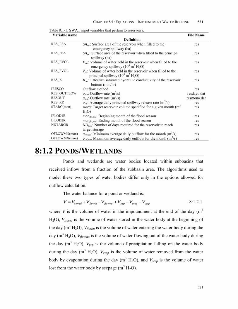
CHAPTER 8:1: EQUATIONS—IMPOUNDMENT WATER ROUTING
521
521
Table 8:1-1: SWAT input variables that pertain to reservoirs. Variable name
Definition File Name
RES_ESA SAem: Surface area of the reservoir when filled to the emergency spillway (ha)
.res
RES_PSA SApr: Surface area of the reservoir when filled to the principal spillway (ha)
.res
RES_EVOL Vem: Volume of water held in the reservoir when filled to the emergency spillway (104 m3 H2O)
.res
RES_PVOL Vpr: Volume of water held in the reservoir when filled to the principal spillway (104 m3 H2O)
.res
RES_K Ksat: Effective saturated hydraulic conductivity of the reservoir bottom (mm/hr)
.res
IRESCO Outflow method .res RES_OUTFLOW qout: Outflow rate (m3/s) resdayo.dat RESOUT qout: Outflow rate (m3/s) resmono.dat RES_RR qrel: Average daily principal spillway release rate (m3/s) .res STARG(mon) starg: Target reservoir volume specified for a given month (m3
H2O) .res
IFLOD1R monfld,beg: Beginning month of the flood season .res IFLOD2R monfld,end: Ending month of the flood season .res NDTARGR NDtarg: Number of days required for the reservoir to reach
target storage .res
OFLOWMN(mon) qrel,mn: Minimum average daily outflow for the month (m3/s) .res OFLOWMX(mon) qrel,mx: Maximum average daily outflow for the month (m3/s) .res
8:1.2 PONDS/WETLANDS Ponds and wetlands are water bodies located within subbasins that
received inflow from a fraction of the subbasin area. The algorithms used to
model these two types of water bodies differ only in the options allowed for
outflow calculation.
The water balance for a pond or wetland is:
seepevappcpflowoutflowinstored VVVVVVV 8:1.2.1
where V is the volume of water in the impoundment at the end of the day (m3
H2O), Vstored is the volume of water stored in the water body at the beginning of
the day (m3 H2O), Vflowin is the volume of water entering the water body during the
day (m3 H2O), Vflowout is the volume of water flowing out of the water body during
the day (m3 H2O), Vpcp is the volume of precipitation falling on the water body
during the day (m3 H2O), Vevap is the volume of water removed from the water
body by evaporation during the day (m3 H2O), and Vseep is the volume of water
lost from the water body by seepage (m3 H2O).
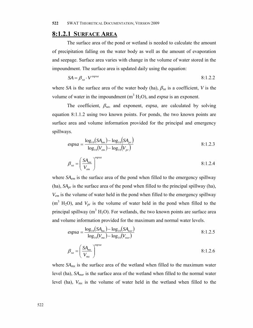
522 SWAT THEORETICAL DOCUMENTATION, VERSION 2009
522
8:1.2.1 SURFACE AREA The surface area of the pond or wetland is needed to calculate the amount
of precipitation falling on the water body as well as the amount of evaporation
and seepage. Surface area varies with change in the volume of water stored in the
impoundment. The surface area is updated daily using the equation:
expsa
sa VSA 8:1.2.2
where SA is the surface area of the water body (ha), sa is a coefficient, V is the
volume of water in the impoundment (m3 H2O), and expsa is an exponent.
The coefficient, sa, and exponent, expsa, are calculated by solving
equation 8:1.1.2 using two known points. For ponds, the two known points are
surface area and volume information provided for the principal and emergency
spillways.
prem
prem
VV
SASAexpsa
1010
1010
loglogloglog
8:1.2.3
expsa
em
emsa
V
SA
8:1.2.4
where SAem is the surface area of the pond when filled to the emergency spillway
(ha), SApr is the surface area of the pond when filled to the principal spillway (ha),
Vem is the volume of water held in the pond when filled to the emergency spillway
(m3 H2O), and Vpr is the volume of water held in the pond when filled to the
principal spillway (m3 H2O). For wetlands, the two known points are surface area
and volume information provided for the maximum and normal water levels.
normx
normx
VV
SASAexpsa
1010
1010
loglogloglog
8:1.2.5
expsa
mx
mxsa
V
SA
8:1.2.6
where SAmx is the surface area of the wetland when filled to the maximum water
level (ha), SAnor is the surface area of the wetland when filled to the normal water
level (ha), Vmx is the volume of water held in the wetland when filled to the

CHAPTER 8:1: EQUATIONS—IMPOUNDMENT WATER ROUTING
523
523
maximum water level (m3 H2O), and Vnor is the volume of water held in the
wetland when filled to the normal water level (m3 H2O).
8:1.2.2 PRECIPITATION The volume of precipitation falling on the pond or wetland during a given
day is calculated:
SARV daypcp 10 8:1.2.7
where Vpcp is the volume of water added to the water body by precipitation during
the day (m3 H2O), Rday is the amount of precipitation falling on a given day (mm
H2O), and SA is the surface area of the water body (ha).
8:1.2.3 INFLOW The volume of water entering the pond or wetland on a given day is
calculated:
SAAreaQQQfrV latgwsurfimpflowin 10 8:1.2.8
where Vflowin is the volume of water flowing into the water body on a given day
(m3 H2O), frimp is the fraction of the subbasin area draining into the impoundment,
Qsurf is the surface runoff from the subbasin on a given day (mm H2O), Qgw is the
groundwater flow generated in a subbasin on a given day (mm H2O), Qlat is the
lateral flow generated in a subbasin on a given day (mm H2O), Area is the
subbasin area (ha), and SA is the surface area of the water body (ha). The volume
of water entering the pond or wetland is subtracted from the surface runoff, lateral
flow and groundwater loadings to the main channel.
8:1.2.4 EVAPORATION The volume of water lost to evaporation on a given day is calculated:
SAEV oevap 10 8:1.2.9
where Vevap is the volume of water removed from the water body by evaporation
during the day (m3 H2O), is an evaporation coefficient (0.6), Eo is the potential
evapotranspiration for a given day (mm H2O), and SA is the surface area of the
water body (ha).

524 SWAT THEORETICAL DOCUMENTATION, VERSION 2009
524
8:1.2.5 SEEPAGE The volume of water lost by seepage through the bottom of the pond or
wetland on a given day is calculated:
SAKV satseep 240 8:1.2.10
where Vseep is the volume of water lost from the water body by seepage (m3 H2O),
Ksat is the effective saturated hydraulic conductivity of the pond or wetland
bottom (mm/hr), and SA is the surface area of the water body (ha).
8:1.2.6 OUTFLOW The primary difference between ponds and wetlands is the method in
which the outflow is calculated.
8:1.2.6.1 POND OUTFLOW Pond outflow is calculated as a function of target storage. The
target storage varies based on flood season and soil water content. The
target pond volume is calculated:
emtarg VV if
endfldbegfld monmonmon ,, 8:1.2.11
premprtarg VVFC
SW
VV
2
1,min1
if begfldmonmon , or
endfldmonmon , 8:1.2.12
where Vtarg is the target pond volume for a given day (m3 H2O), Vem is the volume of water held in the pond when filled to the emergency spillway (m3 H2O), Vpr is the volume of water held in the pond when filled to the principal spillway (m3 H2O), SW is the average soil water content in the subbasin (mm H2O), FC is the water content of the subbasin soil at field capacity (mm H2O), mon is the month of the year, monfld,beg is the beginning month of the flood season, and monfld,end is the ending month of the flood season. Once the target storage is defined, the outflow is calculated:
targ
targ
flowoutND
VVV
8:1.2.13
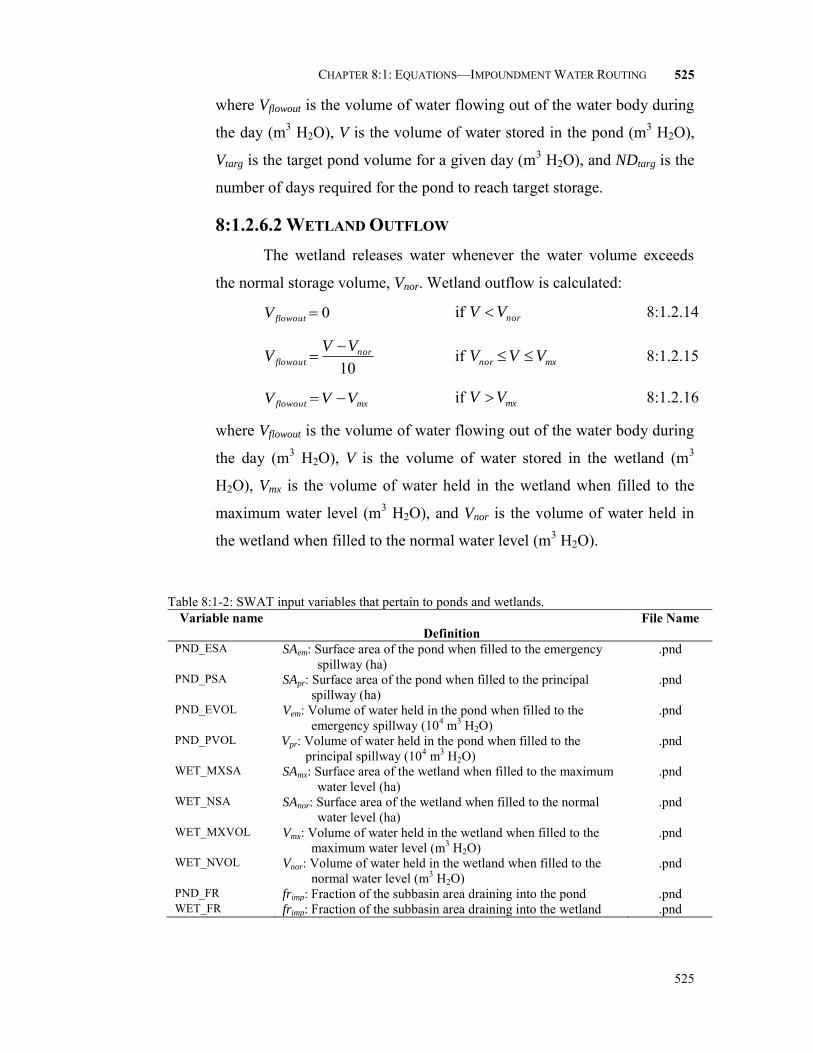
CHAPTER 8:1: EQUATIONS—IMPOUNDMENT WATER ROUTING
525
525
where Vflowout is the volume of water flowing out of the water body during
the day (m3 H2O), V is the volume of water stored in the pond (m3 H2O),
Vtarg is the target pond volume for a given day (m3 H2O), and NDtarg is the
number of days required for the pond to reach target storage.
8:1.2.6.2 WETLAND OUTFLOW The wetland releases water whenever the water volume exceeds
the normal storage volume, Vnor. Wetland outflow is calculated:
0flowoutV if norVV 8:1.2.14
10
norflowout
VVV
if mxnor VVV 8:1.2.15
mxflowout VVV if mxVV 8:1.2.16
where Vflowout is the volume of water flowing out of the water body during
the day (m3 H2O), V is the volume of water stored in the wetland (m3
H2O), Vmx is the volume of water held in the wetland when filled to the
maximum water level (m3 H2O), and Vnor is the volume of water held in
the wetland when filled to the normal water level (m3 H2O).
Table 8:1-2: SWAT input variables that pertain to ponds and wetlands. Variable name
Definition File Name
PND_ESA SAem: Surface area of the pond when filled to the emergency spillway (ha)
.pnd
PND_PSA SApr: Surface area of the pond when filled to the principal spillway (ha)
.pnd
PND_EVOL Vem: Volume of water held in the pond when filled to the emergency spillway (104 m3 H2O)
.pnd
PND_PVOL Vpr: Volume of water held in the pond when filled to the principal spillway (104 m3 H2O)
.pnd
WET_MXSA SAmx: Surface area of the wetland when filled to the maximum water level (ha)
.pnd
WET_NSA SAnor: Surface area of the wetland when filled to the normal water level (ha)
.pnd
WET_MXVOL Vmx: Volume of water held in the wetland when filled to the maximum water level (m3 H2O)
.pnd
WET_NVOL Vnor: Volume of water held in the wetland when filled to the normal water level (m3 H2O)
.pnd
PND_FR frimp: Fraction of the subbasin area draining into the pond .pnd WET_FR frimp: Fraction of the subbasin area draining into the wetland .pnd

526 SWAT THEORETICAL DOCUMENTATION, VERSION 2009
526
Table 8:1-2, cont.: SWAT input variables that pertain to ponds and wetlands Variable name
Definition File Name
PND_K Ksat: Effective saturated hydraulic conductivity of the pond bottom (mm/hr)
.pnd
WET_K Ksat: Effective saturated hydraulic conductivity of the wetland bottom (mm/hr)
.pnd
IFLOD1 monfld,beg: Beginning month of the flood season .pnd IFLOD2 monfld,end: Ending month of the flood season .pnd NDTARG NDtarg: Number of days required for the reservoir to reach
target storage .pnd
8:1.3 DEPRESSIONS/POTHOLES In areas of low relief and/or young geologic development, the drainage
network may be poorly developed. Watersheds in these areas may have many
closed depressional areas, referred to as potholes. Runoff generated within these
areas flows to the lowest portion of the pothole rather than contributing to flow in
the main channel. Other systems that are hydrologically similar to potholes
include playa lakes and fields that are artifically impounded for rice production.
The algorithms reviewed in this section are used to model these types of systems.
To define an HRU as a pothole, the user must set IPOT (.hru) to the HRU
number. To initiate water impoundment, a release/impound operation must be
placed in the .mgt file. The water balance for a pothole is:
seepevappcpflowoutflowinstored VVVVVVV 8:1.3.1
where V is the volume of water in the impoundment at the end of the day (m3
H2O), Vstored is the volume of water stored in the water body at the beginning of
the day (m3 H2O), Vflowin is the volume of water entering the water body during the
day (m3 H2O), Vflowout is the volume of water flowing out of the water body during
the day (m3 H2O), Vpcp is the volume of precipitation falling on the water body
during the day (m3 H2O), Vevap is the volume of water removed from the water
body by evaporation during the day (m3 H2O), and Vseep is the volume of water
lost from the water body by seepage (m3 H2O).
8:1.3.1 SURFACE AREA The surface area of the pothole is needed to calculate the amount of
precipitation falling on the water body as well as the amount of evaporation and
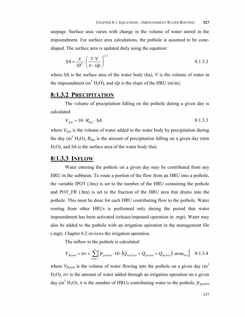
CHAPTER 8:1: EQUATIONS—IMPOUNDMENT WATER ROUTING
527
527
seepage. Surface area varies with change in the volume of water stored in the
impoundment. For surface area calculations, the pothole is assumed to be cone-
shaped. The surface area is updated daily using the equation:
3/2
43
10
slp
VSA
8:1.3.2
where SA is the surface area of the water body (ha), V is the volume of water in
the impoundment (m3 H2O), and slp is the slope of the HRU (m/m).
8:1.3.2 PRECIPITATION The volume of precipitation falling on the pothole during a given day is
calculated:
SARV daypcp 10 8:1.3.3
where Vpcp is the volume of water added to the water body by precipitation during
the day (m3 H2O), Rday is the amount of precipitation falling on a given day (mm
H2O), and SA is the surface area of the water body (ha).
8:1.3.3 INFLOW Water entering the pothole on a given day may be contributed from any
HRU in the subbasin. To route a portion of the flow from an HRU into a pothole,
the variable IPOT (.hru) is set to the number of the HRU containing the pothole
and POT_FR (.hru) is set to the fraction of the HRU area that drains into the
pothole. This must be done for each HRU contributing flow to the pothole. Water
routing from other HRUs is performed only during the period that water
impoundment has been activated (release/impound operation in .mgt). Water may
also be added to the pothole with an irrigation operation in the management file
(.mgt). Chapter 6:2 reviews the irrigation operation.
The inflow to the pothole is calculated:
n
hru
hruhrulathrugwhrusurfhrupotflowin areaQQQfrirrV1
,,,, 10 8:1.3.4
where Vflowin is the volume of water flowing into the pothole on a given day (m3
H2O), irr is the amount of water added through an irrigation operation on a given
day (m3 H2O), n is the number of HRUs contributing water to the pothole, frpot,hru

528 SWAT THEORETICAL DOCUMENTATION, VERSION 2009
528
is the fraction of the HRU area draining into the pothole, Qsurf,hru is the surface
runoff from the HRU on a given day (mm H2O), Qgw,hru is the groundwater flow
generated in the HRU on a given day (mm H2O), Qlat,hru is the lateral flow
generated in the HRU on a given day (mm H2O), and areahru is the HRU area
(ha).
8:1.3.4 EVAPORATION The volume of water lost to evaporation on a given day is calculated:
SAELAI
LAIV o
evap
evap
15 if
evapLAILAI 8:1.3.5
0evapV if evapLAILAI 8:1.3.6
where Vevap is the volume of water removed from the water body by evaporation
during the day (m3 H2O), LAI is the leaf area index of the plants growing in the
pothole, LAIevap is the leaf area index at which no evaporation occurs from the
water surface, Eo is the potential evapotranspiration for a given day (mm H2O),
and SA is the surface area of the water body (ha).
8:1.3.5 SEEPAGE The volume of water lost by seepage through the bottom of the pothole on
a given day is calculated as a function of the water content of the soil profile
beneath the pothole.
SAKV satseep 240 if FCSW 5.0 8:1.3.7
SAKFC
SWV satseep
1240 if FCSWFC 5.0 8:1.3.8
0seepV if FCSW 8:1.3.9
where Vseep is the volume of water lost from the water body by seepage (m3 H2O),
Ksat is the effective saturated hydraulic conductivity of the 1st soil layer in the
profile (mm/hr), SA is the surface area of the water body (ha), SW is the soil water
content of the profile on a given day (mm H2O), and FC is the field capacity soil
water content (mm H2O). Water lost from the pothole by seepage is added to the
soil profile.

CHAPTER 8:1: EQUATIONS—IMPOUNDMENT WATER ROUTING
529
529
8:1.3.6 OUTFLOW Water may be removed from the pothole in three different types of
outflow. When the volume of water in the pothole exceeds the maximum storage,
the excess water is assumed to overflow and enter the main channel in the
subbasin. When the retaining wall or berm is removed (this is done with a
release/impound operation in the management file), all water stored in the pothole
enters the main channel. The third type of flow from the pothole is via drainage
tiles installed in the pothole.
8:1.3.6.1 OVERFLOW Pothole outflow caused by overflow is calculated:
mxpotflowout VVV , if
mxpotVV . 8:1.3.10
where Vflowout is the volume of water flowing out of the water body during
the day (m3 H2O), V is the volume of water stored in the pothole (m3
H2O), and Vpot,mx is the maximum amount of water that can be stored in the
pothole (m3 H2O).
8:1.3.6.2 RELEASE OPERATION When a release operation is scheduled, all water in the pothole
becomes outflow:
VV flowout 8:1.3.11
where Vflowout is the volume of water flowing out of the water body during
the day (m3 H2O), and V is the volume of water stored in the pothole (m3
H2O).
8:1.3.6.3 TILE FLOW When drainage tiles are installed in a pothole, the pothole will
contribute water to the main channel through tile flow. The pothole
outflow originating from tile drainage is:
86400 tileflowout qV if 86400 tileqV 8:1.3.12
VV flowout if 86400 tileqV 8:1.3.13
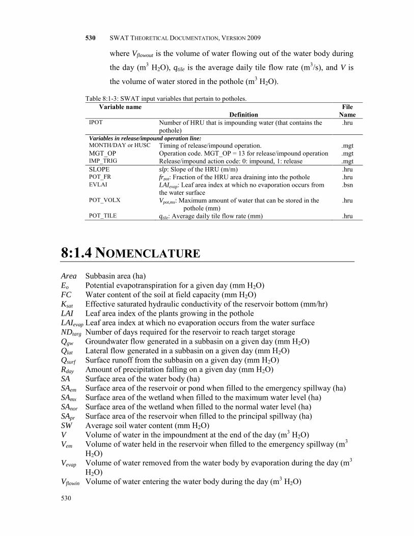
530 SWAT THEORETICAL DOCUMENTATION, VERSION 2009
530
where Vflowout is the volume of water flowing out of the water body during
the day (m3 H2O), qtile is the average daily tile flow rate (m3/s), and V is
the volume of water stored in the pothole (m3 H2O).
Table 8:1-3: SWAT input variables that pertain to potholes. Variable name
Definition File
Name IPOT Number of HRU that is impounding water (that contains the
pothole) .hru
Variables in release/impound operation line: MONTH/DAY or HUSC Timing of release/impound operation. .mgt MGT_OP Operation code. MGT_OP = 13 for release/impound operation .mgt IMP_TRIG Release/impound action code: 0: impound, 1: release .mgt SLOPE slp: Slope of the HRU (m/m) .hru POT_FR frpot: Fraction of the HRU area draining into the pothole .hru EVLAI LAIevap: Leaf area index at which no evaporation occurs from
the water surface .bsn
POT_VOLX Vpot,mx: Maximum amount of water that can be stored in the pothole (mm)
.hru
POT_TILE qtile: Average daily tile flow rate (mm) .hru
8:1.4 NOMENCLATURE Area Subbasin area (ha) Eo Potential evapotranspiration for a given day (mm H2O) FC Water content of the soil at field capacity (mm H2O) Ksat Effective saturated hydraulic conductivity of the reservoir bottom (mm/hr) LAI Leaf area index of the plants growing in the pothole LAIevap Leaf area index at which no evaporation occurs from the water surface
NDtarg Number of days required for the reservoir to reach target storage
Qgw Groundwater flow generated in a subbasin on a given day (mm H2O) Qlat Lateral flow generated in a subbasin on a given day (mm H2O) Qsurf Surface runoff from the subbasin on a given day (mm H2O) Rday Amount of precipitation falling on a given day (mm H2O) SA Surface area of the water body (ha) SAem Surface area of the reservoir or pond when filled to the emergency spillway (ha) SAmx Surface area of the wetland when filled to the maximum water level (ha) SAnor Surface area of the wetland when filled to the normal water level (ha) SApr Surface area of the reservoir when filled to the principal spillway (ha) SW Average soil water content (mm H2O) V Volume of water in the impoundment at the end of the day (m3 H2O) Vem Volume of water held in the reservoir when filled to the emergency spillway (m3
H2O) Vevap Volume of water removed from the water body by evaporation during the day (m3
H2O) Vflowin Volume of water entering the water body during the day (m3 H2O)

CHAPTER 8:1: EQUATIONS—IMPOUNDMENT WATER ROUTING
531
531
Vflowout Volume of water flowing out of the water body during the day (m3 H2O) flowoutV Initial estimate of the volume of water flowing out of the water body during the
day (m3 H2O) Vmx Volume of water held in the wetland when filled to the maximum water level (m3
H2O) Vnor Volume of water held in the wetland when filled to the normal water level (m3
H2O) Vpcp Volume of precipitation falling on the water body during the day (m3 H2O) Vpot,mx Maximum amount of water that can be stored in the pothole (m3 H2O) Vpr Volume of water held in the reservoir when filled to the principal spillway (m3
H2O) Vseep Volume of water lost from the water body by seepage (m3 H2O) Vstored Volume of water stored in the water body at the beginning of the day (m3 H2O) Vtarg Target reservoir volume for a given day (m3 H2O)
areahru HRU area (ha) expsa Exponent for impoundment surface area calculation
frimp Fraction of the subbasin area draining into the impoundment frpot Fraction of the HRU area draining into the pothole
irr Amount of irrigation water added on a given day (m3 H2O) mon Month of the year monfld,beg Beginning month of the flood season monfld,end Ending month of the flood season
qout Outflow rate (m3/s) qrel Average daily principal spillway release rate (m3/s) qrel,mn Minimum average daily outflow for the month (m3/s) qrel,mx Maximum average daily outflow for the month (m3/s) qtile Average daily tile flow rate (m3/s) slp Slope of the HRU (m/m) starg Target reservoir volume specified for a given month (m3 H2O)
sa Coefficient for impoundment surface area equation Evaporation coefficient (0.6)
8:1.5 REFERENCES
Ward, A.D. and W.J. Elliot. 1995. Environmental hydrology. Lewis Publishers,
CRC Press, Inc., Boca Raton, FL.

532 SWAT THEORETICAL DOCUMENTATION, VERSION 2009
532

533
SECTION 8 CHAPTER 2
EQUATIONS:
SEDIMENT IN WATER BODIES
SWAT incorporates a simple mass balance model to simulate the transport
of sediment into and out of water bodies. SWAT defines four different types of
water bodies: ponds, wetlands, reservoirs and potholes. Sediment processes
modeled in ponds, wetlands, reservoirs, and potholes are identical.
When calculating sediment movement through a water body, SWAT
assumes the system is completely mixed. In a completely mixed system, as
sediment enters the water body it is instantaneously distributed throughout the
volume.

534 SWAT THEORETICAL DOCUMENTATION, VERSION 2009
534
8:2.1 MASS BALANCE
The mass balance equation for sediment in a water body is:
flowoutstlflowiniwbwb sedsedsedsedsed , 8:2.1.1
where sedwb is the amount of sediment in the water body at the end of the day
(metric tons), sedwb,i is the amount of sediment in the water body at the beginning
of the day (metric tons), sedflowin is the amount of sediment added to the water
body with inflow (metric tons), sedstl is the amount of sediment removed from the
water by settling (metric tons), sedflowout is the amount of sediment transported out
of the water body with outflow (metric tons).
8:2.2 SETTLING Incoming sediment is deposited using a modified overflow rate model
(EPA 1986, cited in Haan et al., 1994). For each day, the deposition routine
begins with the computation of the detention times. The actual detention time is
based upon the ratio of the impoundment volume to the outflow rate.
o
t
DQ
VolDSCt
)1( 8:2.2.1
Where tD is detention time (s), Ct is an empirical parameter to account for
impoundment geometry, hydraulic response, and stratification of the suspended
sediment, DS is the dead storage (the portion of the pond are that does not
contribute to settling) (Griffin et al., 1985), Vol is the average impoundment
volume over the time step (ft3), and Qo is the average outflow rate over the time
step (ft3 s
-1). The detention time required for 100% of the suspended sediment to
settle out of suspension is computed form the average impoundment depth
(volume / area) and the settling velocity.
The trapping efficiency is calculated as
ovflset VVtrappeff / 8:2.2.2

CHAPTER 8:2: EQUATIONS—SEDIMENT IN WATER BODIES
535
535
Where trapeff is trapping efficiency (fraction), Vsetl is the settling velocity (m/d),
Vovfl is overflow velocity (m/d). Vovfl is defined as
000,10
/ resoovfl
SAQV 8:2.2.3
Where Qo is reservoir outflow in m3 and SAres is reservoir surface area in ha.
During days of no sediment inflow the amount of suspended solid settling
that occurs in the water body on a given day is calculated as a function of
concentration. The initial suspended solid concentration is:
flowinstored
flowiniwb
isedVV
sedsedconc
,, 8:2.2.4
where concsed,i is the initial concentration of suspended solids in the water
(Mg/m3), sedwb,i is the amount of sediment in the water body at the beginning of
the day (metric tons), sedflowin is the amount of sediment added to the water body
with inflow (metric tons), Vstored is the volume of water stored in water body or
channel at the beginning of the day (m3 H2O), and Vflowin is the volume of water
entering water body on given day (m3 H2O).
Settling occurs only when the sediment concentration in the water body
exceeds the equilibrium sediment concentration specified by the user, concsed,eq.
The concentration of sediment in the water body at the end of the day is
calculated:
eqsedseqsedisedfsed concdtkconcconcconc ,50,,, exp
if eqsedised concconc ,, 8:2.2.5
isedfsed concconc ,, if eqsedised concconc ,, 8:2.2.6
where concsed,f is the final sediment concentration in the water body (Mg/m3),
concsed,i is the initial concentration of suspended solids in the water body
(Mg/m3), concsed,eq is the equilibrium concentration of suspended solids in the
water body (Mg/m3), ks is the decay constant (1/day), t is the length of the time
step (1 day), and d50 is the median particle size of the inflow sediment (µm).
Assuming 99% of the 1 µm size particles settle out of solution within 25 days, ks
is equal to 0.184.

536 SWAT THEORETICAL DOCUMENTATION, VERSION 2009
536
For ponds, wetlands, and potholes, the median particle size of the inflow
sediment is calculated:
100
7.5100
71.2100
41.0exp50ssiltc mmm
d 8:2.2.7
where d50 is the median particle size of the inflow sediment (µm), mc is percent
clay in the surface soil layer in the subbasin, msilt is the percent silt in the surface
soil layer in the subbasin, ms is the percent sand in the surface soil layer in the
subbasin. Because reservoirs are located on the main channel network and receive
sediment from the entire area upstream, defaulting the sand, silt, and clay
fractions to those of a single subbasin or HRU in the upstream area is not
appropriate. Instead the user is allowed to set the median particle size diameter to
a representative value for reservoirs.
The amount of sediment settling out of solution on a given day is then
calculated:
Vconcconcsed fsedisedstl ,, 8:2.2.8
where sedstl is the amount of sediment removed from the water by settling (metric
tons), concsed,i is the initial concentration of suspended solids in the water body
(Mg/m3), concsed,f is the final sediment concentration in the water body (Mg/m3),
and V is the volume of water in the impoundment (m3 H2O).
Table 8:2-1: SWAT input variables that pertain to sediment settling. Variable
Name
Definition Input File
RES_NSED concsed,eq: Equilibrium sediment concentration in water body (mg/L) .res PND_NSED concsed,eq: Equilibrium sediment concentration in water body (mg/L) .pnd WET_NSED concsed,eq: Equilibrium sediment concentration in water body (mg/L) .pnd POT_NSED concsed,eq: Equilibrium sediment concentration in water body (mg/L) .hru CLAY mc: Percent clay in the surface soil layer in the subbasin .sol SILT msilt: Percent silt in the surface soil layer in the subbasin .sol SAND ms: Percent sand in the surface soil layer in the subbasin .sol RES_D50 d50: Median particle size of sediment in a reservoir .res

CHAPTER 8:2: EQUATIONS—SEDIMENT IN WATER BODIES
537
537
8:2.3 SEDIMENT OUTFLOW The amount of sediment transported out of the water body on a given day
is calculated as a function of the final concentration. The initial suspended solid
concentration is:
flowoutfsedflowout Vconcsed , 8:2.3.1
where sedflowout is the amount of sediment transported out of the water body with
outflow (metric tons), concsed,f is the final sediment concentration in the water
body (Mg/m3), and Vflowout is the volume of outflow from the impoundment (m3
H2O).
8:2.4 NOMENCLATURE V Volume of water in the impoundment (m3 H2O) Vflowin Volume of water entering water body on given day (m3 H2O) Vflowout Volume of outflow from the impoundment (m3 H2O) Vstored Volume of water stored in water body or channel (m3 H2O)
concsed Concentration of suspended solids in the water (Mg/m3) concsed,eq Equilibrium concentration of suspended solids in the water body (Mg/m3) d50 Median particle size of the inflow sediment (µm) ks Decay constant (1/day) t Length of the time step (1 day) mc Percent clay in the surface soil layer in the subbasin ms Percent sand in the surface soil layer in the subbasin
msilt Percent silt in the surface soil layer in the subbasin sedflowin Amount of sediment added to the water body with inflow (metric tons) sedflowout Amount of sediment transported out of the water body (metric tons) sedstl Amount of sediment removed from the water by settling (metric tons) sedwb Sediment in the water body (metric tons)
8:2.5 REFERENCES
Haan, C.T., B.J. Barfield, and J.C. Hayes. 1994. Design Hydrology and Sedimentology for Small Catchments. Academic Press, New York.
Griffin, M.L., B.J. Barfield, and R.C. Warner. 1985. Laboratory studies of dead
storage in sediment ponds. Transactions of the ASAE 28(3):799-804.

538 SWAT THEORETICAL DOCUMENTATION, VERSION 2009
538
539
SECTION 8 CHAPTER 3
EQUATIONS:
NUTRIENTS IN WATER BODIES
SWAT incorporates a simple empirical model to predict the trophic status
of water bodies. For studies that require detailed modeling of lake water quality,
SWAT has been linked to distributed lake water quality models such as WASP.
SWAT defines four different types of water bodies: ponds, wetlands,
reservoirs and depressional/impounded areas (potholes). Nutrient processes
modeled in ponds, wetlands and reservoirs are identical. Nutrient processes are
not yet modeled in potholes.

540 SWAT THEORETICAL DOCUMENTATION, VERSION 2009
540
8:3.1 NUTRIENT TRANSFORMATIONS
When calculating nutrient transformations in a water body, SWAT
assumes the system is completely mixed. In a completely mixed system, as
nutrients enter the water body they are instantaneously distributed throughout the
volume. The assumption of a completely mixed system ignores lake stratification
and intensification of phytoplankton in the epilimnion.
The initial amount of nitrogen and phosphorus in the water body on the
given day is calculated by summing the mass of nutrient entering the water body
on that day with the mass of nutrient already present in the water body.
flowinstoredinitial MMM 8:3.1.1
where Minitial is the initial mass of nutrient in the water body for the given day
(kg), Mstored is the mass of nutrient in the water body at the end of the previous
day (kg), and Mflowin is the mass of nutrient added to the water body on the given
day (kg).
In a similar manner, the initial volume of water in the water body is
calculated by summing the volume of water entering the water body on that day
with the volume already present in the water body.
flowinstoredinitial VVV 8:3.1.2
where Vinitial is the initial volume of water in the water body for a given day (m3
H2O), Vstored is the volume of water in the water body at the end of the previous
day (m3 H2O), and Vflowin is the volume of water entering the water body on the
given day (m3 H2O).
The initial concentration of nutrients in the water body is calculated by
dividing the initial mass of nutrient by the initial volume of water.
Nutrient transformations simulated in ponds, wetlands and reservoirs are
limited to the removal of nutrients by settling. Transformations between nutrient
pools (e.g. NO3 NO2 NH4) are ignored.

CHAPTER 8:3: EQUATIONS—NUTRIENTS IN WATER BODIES
541
541
Settling losses in the water body can be expressed as a flux of mass across
the surface area of the sediment-water interface (Figure 8:3-1) (Chapra, 1997).
Figure 8:3-1: Settling losses calculated as flux of mass across the sediment-water interface.
The mass of nutrient lost via settling is calculated by multiplying the flux
by the area of the sediment-water interface.
dtAcM ssettling 8:3.1.3
where Msettling is the mass of nutrient lost via settling on a day (kg), is the
apparent settling velocity (m/day), As is the area of the sediment-water interface
(m2), c is the initial concentration of nutrient in the water (kg/m3 H2O), and dt is
the length of the time step (1 day). The settling velocity is labeled as ―apparent‖
because it represents the net effect of the different processes that deliver nutrients
to the water body’s sediments. The water body is assumed to have a uniform
depth of water and the area of the sediment-water interface is equivalent to the
surface area of the water body.
The apparent settling velocity is most commonly reported in units of
m/year and this is how the values are input to the model. For natural lakes,
measured phosphorus settling velocities most frequently fall in the range of 5 to
20 m/year although values less than 1 m/year to over 200 m/year have been
reported (Chapra, 1997). Panuska and Robertson (1999) noted that the range in
apparent settling velocity values for man-made reservoirs tends to be significantly
greater than for natural lakes. Higgins and Kim (1981) reported phosphorus

542 SWAT THEORETICAL DOCUMENTATION, VERSION 2009
542
apparent settling velocity values from –90 to 269 m/year for 18 reservoirs in
Tennessee with a median value of 42.2 m/year. For 27 Midwestern reservoirs,
Walker and Kiihner (1978) reported phosphorus apparent settling velocities
ranging from –1 to 125 m/year with an average value of 12.7 m/year. A negative
settling rate indicates that the reservoir sediments are a source of N or P; a
positive settling rate indicates that the reservoir sediments are a sink for N or P.
A number of inflow and impoundment properties affect the apparent
settling velocity for a water body. Factors of particular importance include the
form of phosphorus in the inflow (dissolved or particulate) and the settling
velocity of the particulate fraction. Within the impoundment, the mean depth,
potential for sediment resuspension and phosphorus release from the sediment
will affect the apparent settling velocity (Panuska and Robertson, 1999). Water
bodies with high internal phosphorus release tend to possess lower phosphorus
retention and lower phosphorus apparent settling velocities than water bodies with
low internal phosphorus release (Nürnberg, 1984). Table 8:3-1 summarizes
typical ranges in phosphorus settling velocity for different systems.
Table 8:3-1: Recommended apparent settling velocity values for phosphorus (Panuska and Robertson, 1999)
Nutrient Dynamics
Range in settling velocity values (m/year)
Shallow water bodies with high net internal phosphorus flux 0 Water bodies with moderate net internal phosphorus flux 1 < < 5 Water bodies with minimal net internal phosphorus flux 5 < < 16 Water bodies with high net internal phosphorus removal > 16
SWAT input variables that pertain to nutrient settling in ponds, wetlands
and reservoirs are listed in Table 8:3-2. The model allows the user to define two
settling rates for each nutrient and the time of the year during which each settling
rate is used. A variation in settling rates is allowed so that impact of temperature
and other seasonal factors may be accounted for in the modeling of nutrient
settling. To use only one settling rate for the entire year, both variables for the
nutrient may be set to the same value. Setting all variables to zero will cause the
model to ignore settling of nutrients in the water body.

CHAPTER 8:3: EQUATIONS—NUTRIENTS IN WATER BODIES
543
543
After nutrient losses in the water body are determined, the final
concentration of nutrients in the water body is calculated by dividing the final
mass of nutrient by the initial volume of water. The concentration of nutrients in
outflow from the water body is equivalent to the final concentration of the
nutrients in the water body for the day. The mass of nutrient in the outflow is
calculated by multiplying the concentration of nutrient in the outflow by the
volume of water leaving the water body on that day.
Table 8:3-2: SWAT input variables that control settling in ponds, wetlands and reservoirs. Variable
Name
Definition Input File
IPND1 Beginning month of mid-year nutrient settling period for pond and wetland modeled in subbasin
.pnd
IPND2 Ending month of mid-year nutrient settling period for pond and wetland modeled in subbasin
.pnd
PSETL1 Phosphorus settling rate in pond during mid-year nutrient settling period (IPND1 month IPND2) (m/year)
.pnd
PSETL2 Phosphorus settling rate in pond during time outside mid-year nutrient settling period ( month < IPND1 or month > IPND2) (m/year)
.pnd
NSETL1 Nitrogen settling rate in pond during mid-year nutrient settling period (IPND1 month IPND2) (m/year)
.pnd
NSETL2 Nitrogen settling rate in pond during time outside mid-year nutrient settling period ( month < IPND1 or month > IPND2) (m/year)
.pnd
PSETLW1 Phosphorus settling rate in wetland during mid-year nutrient settling period (IPND1 month IPND2) (m/year)
.pnd
PSETLW2 Phosphorus settling rate in wetland during time outside mid-year nutrient settling period ( month < IPND1 or month > IPND2) (m/year)
.pnd
NSETLW1 Nitrogen settling rate in wetland during mid-year nutrient settling period (IPND1 month IPND2) (m/year)
.pnd
NSETLW2 Nitrogen settling rate in wetland during time outside mid-year nutrient settling period ( month < IPND1 or month > IPND2) (m/year)
.pnd
IRES1 Beginning month of mid-year nutrient settling period for reservoir .lwq IRES2 Ending month of mid-year nutrient settling period for reservoir .lwq PSETLR1 Phosphorus settling rate in reservoir during mid-year nutrient settling
period (IRES1 month IRES2) (m/year) .lwq
PSETLR2 Phosphorus settling rate in reservoir during time outside mid-year nutrient settling period ( month < IRES1 or month > IRES2) (m/year)
.lwq
NSETLR1 Nitrogen settling rate in reservoir during mid-year nutrient settling period (IRES1 month IRES2) (m/year)
.lwq
NSETLR2 Nitrogen settling rate in reservoir during time outside mid-year nutrient settling period ( month < IRES1 or month > IRES2) (m/year)
.lwq
544 SWAT THEORETICAL DOCUMENTATION, VERSION 2009
544
8:3.2 TOTAL BALANCE Assuming that the volume of the water body remains constant over time,
the processes described above (inflow, settling, outflow) can be combined into the
following mass balance equation for a well-mixed water body:
sAccQtWdt
dcV 8:3.2.1
where V is the volume of the system (m3 H2O), c is the concentration of nutrient
in the system (kg/m3 H2O), dt is the length of the time step (1 day), W(t) is the
amount of nutrient entering the water body during the day (kg/day), Q is the rate
of water flow exiting the water body (m3 H2O/day), is the apparent settling
velocity (m/day), and As is the area of the sediment-water interface (m2).
8:3.3 EUTROPHICATION Under favorable conditions of light and temperature, excess amounts of
nutrients in water can increase the growth of algae and other plants. The result of
this growth is an increase in the rate of eutrophication, which is a natural
ecological process of change from a nutrient-poor to a nutrient-rich environment.
Eutrophication is defined as the process by which a body of water becomes
enriched in dissolved nutrients (as phosphates) that stimulate the growth of
aquatic plant life, usually resulting in the depletion of dissolved oxygen
(Merriam-Webster, Inc., 1996).
Nutrient enrichment of moving waters and lakes is a normal result of soil
weathering and erosion processes. The gradual evolution of Ice Age lakes into
marshes and, eventually, organic soils is a result of eutrophication. However, this
process can be accelerated by the discharge of wastes containing high levels of
nutrients into lakes or rivers. One example of this is Lake Erie, which is estimated
to have aged the equivalent of 150 natural years in a 15-year span of accelerated
eutrophication.
Excessive plant growth caused by accelerated eutrophication can lead to
stagnation of the water. The stagnation is caused by an increased biological

CHAPTER 8:3: EQUATIONS—NUTRIENTS IN WATER BODIES
545
545
oxygen demand created by decaying plant remains. The result of this increased
oxygen demand is a tendency toward anaerobic conditions and the inability of the
water body to support fish and other aerobic organisms.
Nitrogen, carbon and phosphorus are essential to the growth of aquatic
biota. Due to the difficulty of controlling the exchange of nitrogen and carbon
between the atmosphere and water and fixation of atmospheric nitrogen by some
blue-green algae, attempts to mitigate eutrophication have focused on phosphorus
inputs. In fresh-water systems, phosphorus is often the limiting element. By
controlling phosphorus loading, accelerated eutrophication of lake waters can be
reduced.
In systems where phosphorus is the primary, controllable limiting nutrient
of water body eutrophication, the amount of phosphorus present in the water body
can be used to estimate the amount of eutrophication present in the water body.
8:3.3.1 PHOSPHORUS/CHLOROPHYLL a CORRELATIONS A number of empirically derived equations have been developed to
calculate chlorophyll a level as a function of total phosphorus concentration.
SWAT uses an equation developed by Rast and Lee (1978) to calculate the
chlorophyll a concentration in the water body. 76.0551.0 pChla 8:3.3.1
where Chla is the chlorophyll a concentration (g/L) and p is the total phosphorus
concentration (g/L).
The equation has been modified to include a user-defined coefficient:
76.0551.0 pChlaChla co 8:3.3.2
The user-defined coefficient, Chlaco, is included to allow the user to adjust the
predicted chlorophyll a concentration for limitations of nutrients other than
phosphorus. When Chlaco is set to 1.00, equation 8:3.3.2 is equivalent to equation
8:3.3.1. For most water bodies, the original equation will be adequate.
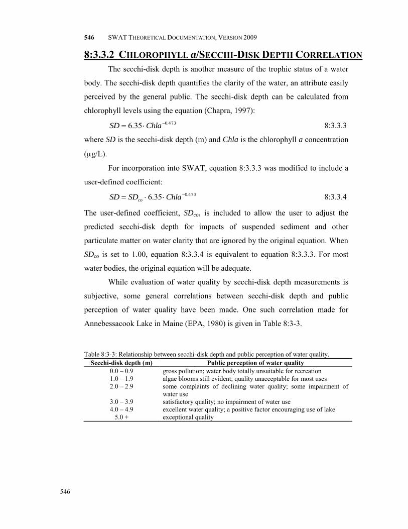
546 SWAT THEORETICAL DOCUMENTATION, VERSION 2009
546
8:3.3.2 CHLOROPHYLL a/SECCHI-DISK DEPTH CORRELATION The secchi-disk depth is another measure of the trophic status of a water
body. The secchi-disk depth quantifies the clarity of the water, an attribute easily
perceived by the general public. The secchi-disk depth can be calculated from
chlorophyll levels using the equation (Chapra, 1997): 473.035.6 ChlaSD 8:3.3.3
where SD is the secchi-disk depth (m) and Chla is the chlorophyll a concentration
(g/L).
For incorporation into SWAT, equation 8:3.3.3 was modified to include a
user-defined coefficient: 473.035.6 ChlaSDSD co 8:3.3.4
The user-defined coefficient, SDco, is included to allow the user to adjust the
predicted secchi-disk depth for impacts of suspended sediment and other
particulate matter on water clarity that are ignored by the original equation. When
SDco is set to 1.00, equation 8:3.3.4 is equivalent to equation 8:3.3.3. For most
water bodies, the original equation will be adequate.
While evaluation of water quality by secchi-disk depth measurements is
subjective, some general correlations between secchi-disk depth and public
perception of water quality have been made. One such correlation made for
Annebessacook Lake in Maine (EPA, 1980) is given in Table 8:3-3.
Table 8:3-3: Relationship between secchi-disk depth and public perception of water quality. Secchi-disk depth (m) Public perception of water quality
0.0 – 0.9 gross pollution; water body totally unsuitable for recreation 1.0 – 1.9 algae blooms still evident; quality unacceptable for most uses 2.0 – 2.9 some complaints of declining water quality; some impairment of
water use 3.0 – 3.9 satisfactory quality; no impairment of water use 4.0 – 4.9 excellent water quality; a positive factor encouraging use of lake
5.0 + exceptional quality

CHAPTER 8:3: EQUATIONS—NUTRIENTS IN WATER BODIES
547
547
Table 8:3-4: SWAT input variables that impact eutrophication calculations in ponds, wetlands and reservoirs.
Variable Name
Definition
Input File
CHLA Chlaco variable for calculation of chlorophyll a concentration in a pond .pnd CHLAW Chlaco variable for calculation of chlorophyll a concentration in a
wetland .pnd
CHLAR Chlaco variable for calculation of chlorophyll a concentration in a reservoir
.lwq
SECCI SDco variable for calculation of secchi-disk depth in a pond .pnd SECCIW SDco variable for calculation of secchi-disk depth in a wetland .pnd SECCIR SDco variable for calculation of secchi-disk depth in a reservoir .lwq
8:3.4 NOMENCLATURE As Area of sediment-water interface (m2) Chla Chlorophyll a concentration (g/L) Chlaco User-defined coefficient to adjust predicted chlorophyll a concentration Mflowin Mass of nutrient entering water body on the given day (kg) Minitial Initial mass of nutrient in water body for the given day (kg) Msettling Mass of nutrient lost via settling on a given day (kg) Mstored Mass of nutrient in water body at end of previous day (kg) Q Volumetric flow rate for water exiting water body (m3 H2O/day) SD Secchi-disk depth (m) SDco User-defined coefficient to adjust predicted secchi-disk depth V Volume of water in water body (assumed constant) (m3 H2O) Vflowin Volume of water entering water body on given day (m3 H2O) Vinitial Initial volume of water in water body on given day (m3 H2O) Vstored Volume of water in water body at end of previous day (m3 H2O) W(t) Rate of nutrient loading (kg/day) c Concentration of nutrient in the water (kg/m3 H2O) dt Length of time step (1 day) p Total phosphorus concentration (g P/L)
Apparent settling velocity (m/day)
8:3.5 REFERENCES
Chapra, S.C. 1997. Surface water-quality modeling. WCB/McGraw-Hill, Boston,
MA.
Higgins, J.M. and B.R. Kim. 1981. Phosphorus retention models for the
Tennessee Valley Authority reservoirs. Wat. Resour. Res. 17:571-576.

548 SWAT THEORETICAL DOCUMENTATION, VERSION 2009
548
Merriam-Webster, Inc. 1996. Merriam-Webster’s collegiate dictionary, 10th
edition. Merriam-Webster, Inc. Springfield, MA.
Nürnberg, G.K. 1984. The prediction of internal phosphorus load in lakes with
anoxic hypolimnia. Limnol. Oceanogr. 29:111-124.
Panuska, J.C. and D.M. Robertson. 1999. Estimating phosphorus concentration
following alum treatment using apparent settling velocity. Lake and
Reserv. Manage. 15:28-38.
Rast, W. and Lee, G.F. 1978. Summary analysis of the North American project
(US portion) OECD eutrophication project: nutrient loading-lake response
relationships and trophic state indices. USEPA Corvallis Environmental
Research Laboratory, Corvallis, OR. EPA-600/3-78-008.
USEPA. 1980. Lake restoration in Cobbossee watershed. Capsule Rept. Office of
Water Planning and Standards Div., ORD, Cincinnati, OH. EPA-624/2-
80-027.
Walker, W.W. and J. Kiihner. 1978. An empirical analysis of factors controlling
eutrophication in midwestern impoundments. Paper presented at the
International Symposium on the Environmental Effects of Hydraulic
Engineering Works, Univ. of Tenn., Knoxville.

CHAPTER 8:3: EQUATIONS—NUTRIENTS IN WATER BODIES
549
549
550
SECTION 8 CHAPTER 4
EQUATIONS:
PESTICIDES IN WATER BODIES
SWAT incorporates a simple mass balance developed by Chapra (1997) to
model the transformation and transport of pesticides in water bodies. The model
assumes a well-mixed layer of water overlying a sediment layer. Figure 8:4-1
illustrates the mechanisms affecting the pesticide mass balance in water bodies.
SWAT defines four different types of water bodies: ponds, wetlands,
reservoirs and depressional/impounded areas (potholes). Pesticide processes are
modeled only in reservoirs.
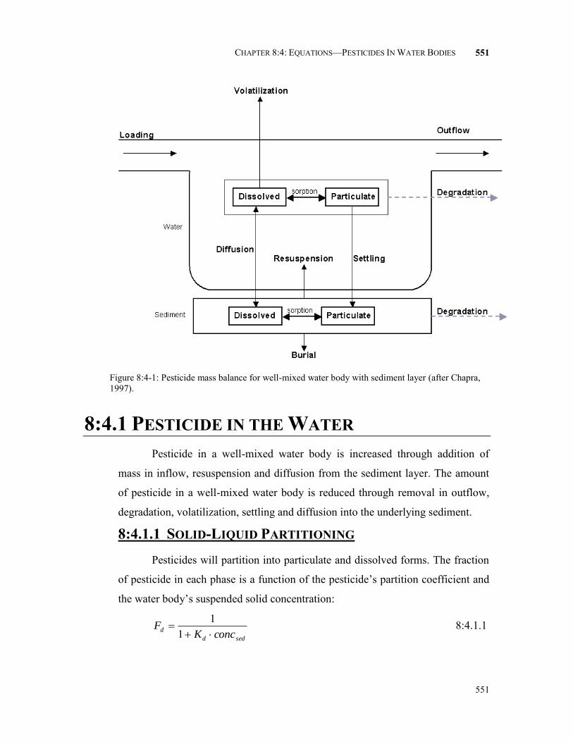
CHAPTER 8:4: EQUATIONS—PESTICIDES IN WATER BODIES
551
551
Figure 8:4-1: Pesticide mass balance for well-mixed water body with sediment layer (after Chapra, 1997).
8:4.1 PESTICIDE IN THE WATER
Pesticide in a well-mixed water body is increased through addition of
mass in inflow, resuspension and diffusion from the sediment layer. The amount
of pesticide in a well-mixed water body is reduced through removal in outflow,
degradation, volatilization, settling and diffusion into the underlying sediment.
8:4.1.1 SOLID-LIQUID PARTITIONING
Pesticides will partition into particulate and dissolved forms. The fraction
of pesticide in each phase is a function of the pesticide’s partition coefficient and
the water body’s suspended solid concentration:
sedd
dconcK
F
1
1 8:4.1.1

552 SWAT THEORETICAL DOCUMENTATION, VERSION 2009
552
d
sedd
seddp F
concK
concKF
1
1 8:4.1.2
where Fd is the fraction of total pesticide in the dissolved phase, Fp is the fraction
of total pesticide in the particulate phase, Kd is the pesticide partition coefficient
(m3/g), and concsed is the concentration of suspended solids in the water (g/m3).
The pesticide partition coefficient can be estimated from the octanol-water
partition coefficient (Chapra, 1997):
owd KK 810085.3 8:4.1.3
where Kd is the pesticide partition coefficient (m3/g) and Kow is the pesticide’s
octanol-water partition coefficient ( 13water
3octanol m mg m mg ). Values for the
octanol-water partition coefficient have been published for many chemicals. If a
published value cannot be found, it can be estimated from solubility (Chapra,
1997):
solow tpsK log670.000.5log 8:4.1.4
where soltps is the pesticide solubility (μmoles/L). The solubility in these units is
calculated:
310MW
psttps sol
sol 8:4.1.5
where soltps is the pesticide solubility (μmoles/L), pstsol is the pesticide solubility
(mg/L) and MW is the molecular weight (g/mole).
8:4.1.2 DEGRADATION Pesticides in both the particulate and dissolved forms are subject to
degradation. The amount of pesticide that is removed from the water via
degradation is:
lkwtraqpdeg,wtr pstkpst , 8:4.1.6
where pstdeg,wtr is the amount of pesticide removed from the water via degradation
(mg pst), kp,aq is the rate constant for degradation or removal of pesticide in the
water (1/day), and pstlkwtr is the amount of pesticide in the water at the beginning
of the day (mg pst). The rate constant is related to the aqueous half-life:

CHAPTER 8:4: EQUATIONS—PESTICIDES IN WATER BODIES
553
553
aq
aqpt
k,2/1
,693.0
8:4.1.7
where kp,aq is the rate constant for degradation or removal of pesticide in the water
(1/day), and t1/2,aq is the aqueous half-life for the pesticide (days).
8:4.1.3 VOLATILIZATION Pesticide in the dissolved phase is available for volatilization. The amount
of pesticide removed from the water via volatilization is:
V
pstFSAvpst lkwtrd
vwtrvol
, 8:4.1.8
where pstvol,wtr is the amount of pesticide removed via volatilization (mg pst), vv is
the volatilization mass-transfer coefficient (m/day), SA is the surface area of the
water body (m2), Fd is the fraction of total pesticide in the dissolved phase, pstlkwtr
is the amount of pesticide in the water (mg pst), and V is the volume of water in
the water body (m3 H2O).
The volatilization mass-transfer coefficient can be calculated based on
Whitman’s two-film or two-resistance theory (Whitman, 1923; Lewis and
Whitman, 1924 as described in Chapra, 1997). While the main body of the gas
and liquid phases are assumed to be well-mixed and homogenous, the two-film
theory assumes that a substance moving between the two phases encounters
maximum resistance in two laminar boundary layers where transfer is a function
of molecular diffusion. In this type of system the transfer coefficient or velocity
is:
glKe
elv
KKTRH
HKv
8:4.1.9
where vv is the volatilization mass-transfer coefficient (m/day), Kl is the mass-
transfer velocity in the liquid laminar layer (m/day), Kg is the mass-transfer
velocity in the gaseous laminar layer (m/day), He is Henry’s constant (atm m3
mole-1), R is the universal gas constant (8.206 10-5 atm m3 (K mole)-1), and TK is
the temperature (K).
For lakes, the transfer coefficients are estimated using a stagnant film
approach:

554 SWAT THEORETICAL DOCUMENTATION, VERSION 2009
554
l
ll
z
DK
g
g
gz
DK 8:4.1.10
where Kl is the mass-transfer velocity in the liquid laminar layer (m/day), Kg is the
mass-transfer velocity in the gaseous laminar layer (m/day), Dl is the liquid
molecular diffusion coefficient (m2/day), Dg is the gas molecular diffusion
coefficient (m2/day), zl is the thickness of the liquid film (m), and zg is the
thickness of the gas film (m).
Alternatively, the transfer coefficients can be estimated with the equations:
25.0
O,32
2
MWKK ll 8:4.1.11
25.018168
MWK wg 8:4.1.12
where Kl is the mass-transfer velocity in the liquid laminar layer (m/day), Kg is the
mass-transfer velocity in the gaseous laminar layer (m/day), 2O,lK is the oxygen
transfer coefficient (m/day), MW is the molecular weight of the compound, and
w is the wind speed (m/s). Chapra (1997) lists several different equations that can
be used to calculate 2O,lK .
8:4.1.4 SETTLING Pesticide in the particulate phase may be removed from the water layer by
settling. Settling transfers pesticide from the water to the sediment layer. The
amount of pesticide that is removed from the water via settling is:
V
lkwtrpst
pF
SAs
vwtrstl
pst
, 8:4.1.13
where pststl,wtr is the amount of pesticide removed from the water due to settling
(mg pst), vs is the settling velocity (m/day), SA is the surface area of the water
body (m2), Fp is the fraction of total pesticide in the particulate phase, pstlkwtr is
the amount of pesticide in the water (mg pst), and V is the volume of water in the
water body (m3 H2O).

CHAPTER 8:4: EQUATIONS—PESTICIDES IN WATER BODIES
555
555
8:4.1.5 OUTFLOW Pesticide is removed from the water body in outflow. The amount of
dissolved and particulate pesticide removed from the water body in outflow is:
V
pstFQpst lkwtrd
osol
, 8:4.1.14
V
pstFQpst
lkwtrp
osorb
, 8:4.1.15
where pstsol,o is the amount of dissolved pesticide removed via outflow (mg pst),
pstsorb,o is the amount of particulate pesticide removed via outflow (mg pst), Q is
the rate of outflow from the water body (m3 H2O/day), Fd is the fraction of total
pesticide in the dissolved phase, Fp is the fraction of total pesticide in the
particulate phase, pstlkwtr is the amount of pesticide in the water (mg pst), and V is
the volume of water in the water body (m3 H2O).
Table 8:4-1: SWAT input variables that pesticide partitioning. Variable
Name
Definition Input File
LKPST_KOC Kd: Pesticide partition coefficient (m3/g) .lwq LKPST_REA kp,aq: Rate constant for degradation or removal of pesticide in the water
(1/day) .lwq
LKPST_VOL vv: Volatilization mass-transfer coefficient (m/day) .lwq LKPST_STL vs: Pesticide settling velocity (m/day) .lwq
8:4.2 PESTICIDE IN THE SEDIMENT
Pesticide in the sediment layer underlying a water body is increased
through addition of mass by settling and diffusion from the water. The amount of
pesticide in the sediment layer is reduced through removal by degradation,
resuspension, diffusion into the overlying water, and burial.
8:4.2.1 SOLID-LIQUID PARTITIONING As in the water layer, pesticides in the sediment layer will partition into
particulate and dissolved forms. Calculation of the solid-liquid partitioning in the
sediment layer requires a suspended solid concentration. The “concentration” of
solid particles in the sediment layer is defined as:
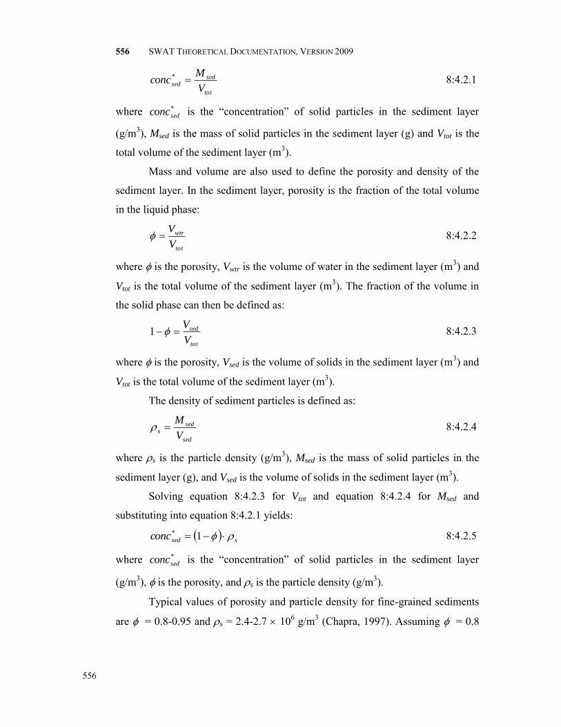
556 SWAT THEORETICAL DOCUMENTATION, VERSION 2009
556
tot
sedsed
V
Mconc * 8:4.2.1
where *sedconc is the “concentration” of solid particles in the sediment layer
(g/m3), Msed is the mass of solid particles in the sediment layer (g) and Vtot is the
total volume of the sediment layer (m3).
Mass and volume are also used to define the porosity and density of the
sediment layer. In the sediment layer, porosity is the fraction of the total volume
in the liquid phase:
tot
wtr
V
V 8:4.2.2
where is the porosity, Vwtr is the volume of water in the sediment layer (m3) and
Vtot is the total volume of the sediment layer (m3). The fraction of the volume in
the solid phase can then be defined as:
tot
sed
V
V1 8:4.2.3
where is the porosity, Vsed is the volume of solids in the sediment layer (m3) and
Vtot is the total volume of the sediment layer (m3).
The density of sediment particles is defined as:
sed
seds
V
M 8:4.2.4
where s is the particle density (g/m3), Msed is the mass of solid particles in the
sediment layer (g), and Vsed is the volume of solids in the sediment layer (m3).
Solving equation 8:4.2.3 for Vtot and equation 8:4.2.4 for Msed and
substituting into equation 8:4.2.1 yields:
ssedconc 1* 8:4.2.5
where *sedconc is the “concentration” of solid particles in the sediment layer
(g/m3), is the porosity, and s is the particle density (g/m3).
Typical values of porosity and particle density for fine-grained sediments
are = 0.8-0.95 and s = 2.4-2.7 106 g/m3 (Chapra, 1997). Assuming = 0.8

CHAPTER 8:4: EQUATIONS—PESTICIDES IN WATER BODIES
557
557
and s = 2.6 106 g/m3, the “concentration” of solid particles in the sediment
layer is 5.2 105 g/m3.
The fraction of pesticide in each phase is then calculated:
ds
seddK
F
1
1, 8:4.2.6
seddsedp FF ,, 1 8:4.2.7
where Fd,sed is the fraction of total sediment pesticide in the dissolved phase, Fp,sed
is the fraction of total sediment pesticide in the particulate phase, is the porosity,
s is the particle density (g/m3), and Kd is the pesticide partition coefficient (m3/g).
The pesticide partition coefficient used for the water layer is also used for the
sediment layer.
8:4.2.2 DEGRADATION Pesticides in both the particulate and dissolved forms are subject to
degradation. The amount of pesticide that is removed from the sediment via
degradation is:
lksedsedpdeg,sed pstkpst , 8:4.2.8
where pstdeg,sed is the amount of pesticide removed from the sediment via
degradation (mg pst), kp,sed is the rate constant for degradation or removal of
pesticide in the sediment (1/day), and pstlksed is the amount of pesticide in the
sediment (mg pst). The rate constant is related to the sediment half-life:
sed
sedpt
k,2/1
,693.0
8:4.2.9
where kp,sed is the rate constant for degradation or removal of pesticide in the
sediment (1/day), and t1/2,sed is the sediment half-life for the pesticide (days).
8:4.2.3 RESUSPENSION Pesticide in the sediment layer is available for resuspension. The amount
of pesticide that is removed from the sediment via resuspension is:
tot
lksedrwtrrsp
V
pstSAvpst , 8:4.2.10

558 SWAT THEORETICAL DOCUMENTATION, VERSION 2009
558
where pstrsp,wtr is the amount of pesticide removed via resuspension (mg pst), vr is
the resuspension velocity (m/day), SA is the surface area of the water body (m2),
pstlksed is the amount of pesticide in the sediment (mg pst), and Vtot is the volume
of the sediment layer (m3). The volume of the sediment layer is calculated:
sedtot DSAV 8:4.2.11
where Vtot is the volume of the sediment layer (m3), SA is the surface area of the
water body (m2), Dsed is the depth of the active sediment layer (m). Pesticide
removed from the sediment layer by resuspension is added to the water layer.
8:4.2.4 DIFFUSION Pesticide in the dissolved phase is available for diffusion. Diffusion
transfers pesticide between the water and sediment layers. The direction of
movement is controlled by the pesticide concentration. Pesticide will move from
areas of high concentration to areas of low concentration. The amount of pesticide
that is transferred between the water and sediment by diffusion is:
V
pstF
V
pstFSAvpst lkwtrd
tot
lksedsedd
ddif
, 8:4.2.12
where pstdif is the amount of pesticide transferred between the water and sediment
by diffusion (mg pst), vd is the rate of diffusion or mixing velocity (m/day), SA is
the surface area of the water body (m2), Fd,sed is the fraction of total sediment
pesticide in the dissolved phase, pstlksed is the amount of pesticide in the sediment
(mg pst), Vtot is the volume of the sediment layer (m3), Fd is the fraction of total
water layer pesticide in the dissolved phase, pstlkwtr is the amount of pesticide in
the water (mg pst), and V is the volume of water in the water body (m3 H2O). If
V
pstF
V
pstFlkwtrd
tot
lksedsedd
, , pstdif is transferred from the sediment to the water
layer. If V
pstF
V
pstFlkwtrd
tot
lksedsedd
, , pstdif is transferred from the water to the
sediment layer.
The diffusive mixing velocity, vd, can be estimated from the empirically
derived formula (Chapra, 1997):
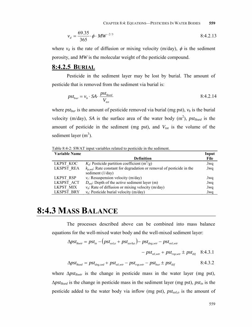
CHAPTER 8:4: EQUATIONS—PESTICIDES IN WATER BODIES
559
559
3/2
36535.69 MWvd 8:4.2.13
where vd is the rate of diffusion or mixing velocity (m/day), is the sediment
porosity, and MW is the molecular weight of the pesticide compound.
8:4.2.5 BURIAL Pesticide in the sediment layer may be lost by burial. The amount of
pesticide that is removed from the sediment via burial is:
tot
lksedbbur
V
pstSAvpst 8:4.2.14
where pstbur is the amount of pesticide removed via burial (mg pst), vb is the burial
velocity (m/day), SA is the surface area of the water body (m2), pstlksed is the
amount of pesticide in the sediment (mg pst), and Vtot is the volume of the
sediment layer (m3).
Table 8:4-2: SWAT input variables related to pesticide in the sediment. Variable Name
Definition Input File
LKPST_KOC Kd: Pesticide partition coefficient (m3/g) .lwq LKSPST_REA kp,sed: Rate constant for degradation or removal of pesticide in the
sediment (1/day) .lwq
LKPST_RSP vr: Resuspension velocity (m/day) .lwq LKSPST_ACT Dsed: Depth of the active sediment layer (m) .lwq LKPST_MIX vd: Rate of diffusion or mixing velocity (m/day) .lwq LKSPST_BRY vb: Pesticide burial velocity (m/day) .lwq
8:4.3 MASS BALANCE The processes described above can be combined into mass balance
equations for the well-mixed water body and the well-mixed sediment layer:
wtrvolwtrdegosorbosolinlkwtr pstpstpstpstpstpst ,,,,
difwtrrspwtrstl pstpstpst ,, 8:4.3.1
difburwtrrspwtrstldeg,sedlksed pstpstpstpstpstpst ,, 8:4.3.2
where pstlkwtr is the change in pesticide mass in the water layer (mg pst),
pstlksed is the change in pesticide mass in the sediment layer (mg pst), pstin is the
pesticide added to the water body via inflow (mg pst), pstsol,o is the amount of

560 SWAT THEORETICAL DOCUMENTATION, VERSION 2009
560
dissolved pesticide removed via outflow (mg pst), pstsorb,o is the amount of
particulate pesticide removed via outflow (mg pst), pstdeg,wtr is the amount of
pesticide removed from the water via degradation (mg pst), pstvol,wtr is the amount
of pesticide removed via volatilization (mg pst), pststl,wtr is the amount of pesticide
removed from the water due to settling (mg pst), pstrsp,wtr is the amount of
pesticide removed via resuspension (mg pst), pstdif is the amount of pesticide
transferred between the water and sediment by diffusion (mg pst), pstdeg,sed is the
amount of pesticide removed from the sediment via degradation (mg pst), pstbur is
the amount of pesticide removed via burial (mg pst)
8:4.4 NOMENCLATURE Dg Gas molecular diffusion coefficient (m2/day) Dl Liquid molecular diffusion coefficient (m2/day) Dsed Depth of the active sediment layer (m) Fd Fraction of total pesticide in the dissolved phase Fd,sed Fraction of total sediment pesticide in the dissolved phase Fp Fraction of total pesticide in the particulate phase Fp,sed Fraction of total sediment pesticide in the particulate phase
He Henry’s constant (atm m3 mole-1) Kd Pesticide partition coefficient (m3/g) Kg Mass-transfer velocity in the gaseous laminar layer (m/day) Kl Mass-transfer velocity in the liquid laminar layer (m/day)
2O,lK Oxygen transfer coefficient (m/day) Msed Mass of solid phase in the sediment layer (g) MW Molecular weight of the pesticide compound
Q Rate of outflow from the water body (m3 H2O/day) R Universal gas constant (8.206 10-5 atm m3 (K mole)-1) SA Surface area of the water body (m2) V Volume of water in the water body (m3 H2O) Vsed Volume of solids in the sediment layer (m3) Vtot Total volume of the sediment layer (m3) Vwtr Volume of water in the sediment layer (m3) concsed Concentration of suspended solids in the water (g/m3)
*sedconc “Concentration” of solid particles in the sediment layer (g/m3)
kp,aq Rate constant for degradation or removal of pesticide in the water (1/day) kp,sed Rate constant for degradation or removal of pesticide in the sediment (1/day) pstbur Amount of pesticide removed via burial (mg pst) pstdeg,sed Amount of pesticide removed from the sediment via degradation (mg pst)

CHAPTER 8:4: EQUATIONS—PESTICIDES IN WATER BODIES
561
561
pstdeg,wtr Amount of pesticide removed from the water via degradation (mg pst) pstdif Amount of pesticide transferred between the water and sediment by diffusion (mg
pst) pstin Pesticide added to the water body via inflow (mg pst) pstlksed Amount of pesticide in the sediment (mg pst) pstlkwtr Amount of pesticide in the water (mg pst) pstrsp,wtr Amount of pesticide removed from sediment via resuspension (mg pst) pstsol,o Amount of dissolved pesticide removed via outflow (mg pst) pstsorb,o Amount of particulate pesticide removed via outflow (mg pst) pststl,wtr Amount of pesticide removed from the water due to settling (mg pst) pstvol,wtr Amount of pesticide removed via volatilization (mg pst) t1/2,aq Aqueous half-life for the pesticide (days) t1/2,sed Sediment half-life for the pesticide (days) vb Pesticide burial velocity (m/day) vd Rate of diffusion or mixing velocity (m/day) vr Resuspension velocity (m/day) vs Settling velocity (m/day) vv Volatilization mass-transfer coefficient (m/day) zg Thickness of the gas film (m) zl Thickness of the liquid film (m) Porosity pstlkwtr Change in pesticide mass in the water layer (mg pst) pstlksed Change in pesticide mass in the sediment layer (mg pst) s Particle density (g/m3) w Wind speed (m/s)
8:4.5 REFERENCES
Chapra, S.C. 1997. Surface water-quality modeling. WCB/McGraw-Hill, Boston,
MA.
Lewis, W.K. and W.G. Whitman. 1924. Principles of gas absorption. Ind. Eng.
Chem. 16:1215-1220.
Whitman, W.G. 1923. The two-film theory of gas adsorption. Chem. Metallurg.
Eng. 29:146-148.

562 SWAT THEORETICAL DOCUMENTATION, VERSION 2009
562

563
SECTION 8 CHAPTER 5
EQUATIONS:
BACTERIA IN WATER BODIES
SWAT calculates loading of pathogens and indicator bacteria for
pathogens from land areas in the watershed. In reservoirs, bacteria die-off is the
only process modeled.
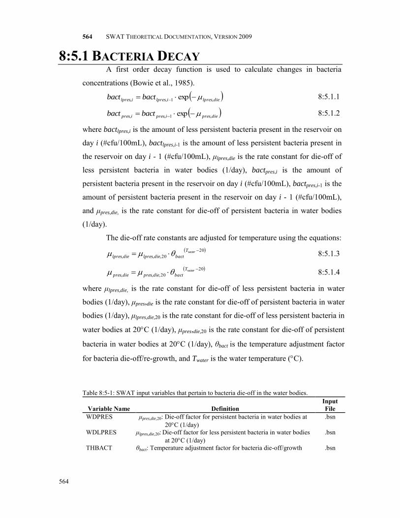
564 SWAT THEORETICAL DOCUMENTATION, VERSION 2009
564
8:5.1 BACTERIA DECAY A first order decay function is used to calculate changes in bacteria
concentrations (Bowie et al., 1985).
dielpresilpresilpres bactbact ,1,, exp
8:5.1.1
diepresipresipres bactbact ,1,, exp
8:5.1.2
where bactlpres,i is the amount of less persistent bacteria present in the reservoir on
day i (#cfu/100mL), bactlpres,i-1 is the amount of less persistent bacteria present in
the reservoir on day i - 1 (#cfu/100mL), μlpres,die is the rate constant for die-off of
less persistent bacteria in water bodies (1/day), bactpres,i is the amount of
persistent bacteria present in the reservoir on day i (#cfu/100mL), bactpres,i-1 is the
amount of persistent bacteria present in the reservoir on day i - 1 (#cfu/100mL),
and μpres,die, is the rate constant for die-off of persistent bacteria in water bodies
(1/day).
The die-off rate constants are adjusted for temperature using the equations: 20
20,,,
waterT
bactdielpresdielpres 8:5.1.3
2020,,,
waterT
bactdiepresdiepres 8:5.1.4
where μlpres,die, is the rate constant for die-off of less persistent bacteria in water
bodies (1/day), μpres,die is the rate constant for die-off of persistent bacteria in water
bodies (1/day), μlpres,die,20 is the rate constant for die-off of less persistent bacteria in
water bodies at 20C (1/day), μpres,die,20 is the rate constant for die-off of persistent
bacteria in water bodies at 20C (1/day), θbact is the temperature adjustment factor
for bacteria die-off/re-growth, and Twater is the water temperature (C).
Table 8:5-1: SWAT input variables that pertain to bacteria die-off in the water bodies.
Variable Name
Definition Input File
WDPRES μpres,die,20: Die-off factor for persistent bacteria in water bodies at 20C (1/day)
.bsn
WDLPRES μlpres,die,20: Die-off factor for less persistent bacteria in water bodies at 20C (1/day)
.bsn
THBACT θbact: Temperature adjustment factor for bacteria die-off/growth .bsn

CHAPTER 7:5: EQUATIONS—BACTERIA ROUTING
565
565
8:5.2 NOMENCLATURE
Twater Average daily water temperature (C) bactlpres Amount of less persistent bacteria present in the reservoir (#cfu/100mL) bactpres Amount of persistent bacteria present in the reservoir (#cfu/100mL)
θbact Temperature adjustment factor for bacteria die-off/re-growth μlpres,die Rate constant for die-off of less persistent bacteria in water bodies (1/day)
μlpres,die,20 Rate constant for die-off of less persistent bacteria in water bodies at 20C (1/day)
μpres,die Rate constant for die-off of persistent bacteria in water bodies (1/day) μpres,die,20 Rate constant for die-off of persistent bacteria in water bodies at 20C (1/day)
8:5.3 REFERENCES
Bowie, G.W., W. Mills, D. Porcella, C. Campbell, J. Pagenkopf, G. Rupp, K.
Johnson, P. Chan, S. Gherini, and C. Chamberlin. 1985. Rates, constants
and kinetics formulations in surface water quality modeling. 2nd ed.
USEPA/600/3-85-040.

566 SWAT THEORETICAL DOCUMENTATION, VERSION 2009
566

567
APPENDIX A
LIST OF VARIABLES

568 SWAT THEORETICAL DOCUMENTATION, VERSION 2009
568
A 3 3 matrix of elements defined to ensure serial and cross correlation of generated temperature and radiation values 1
01
MMA
Ach Cross-sectional area of flow in the channel (m2) Ach,bnkfull Cross-sectional area of flow in the channel when filled to the top of the bank
(m2) Ad Area of drain field (ha) As Area of sediment-water interface (m2) Asurf Amplitude of the surface fluctuations in soil temperature (C) AGP Algal growth potential (mg/L) Area Subbasin area (km2 or ha) AU Astronomical unit (1 AU = 1.496 x 10⁸ km) AWC Available water capacity (mm H2O) AWCly Available water capacity for layer ly (mm H2O) B 3 3 matrix of elements defined to ensure serial and cross correlation of
generated temperature and radiation values TT MMMMBB 11
010
BFD Number of baseflow days for the watershed Bio Amount of live bacteria biomass in biozone (kg/ha) C Runoff coefficient in peak runoff rate calculation C Concentration of the solute in solution in equilibrium with the mass of solute
sorbed onto the solid (mg/L), C1 Coefficient in Muskingum flood routing equation C2 Coefficient in Muskingum flood routing equation C3 Coefficient in Muskingum flood routing equation CBOD,in BOD concentration in STE (mg/L) CBOD BOD concentration in biozone (mg/L) CCH Channel cover factor Ck, end Concentration of k constituent in the biozone at the end of the day (mg/L) Ck, i Concentration of k constituent in the biozone at the beginning of the day (mg/L) CNH4 Concentration of ammonium in the reach (mg N/L) CNO3 Concentration of nitrate in the reach (mg N/L) Csolidphase Concentration of the pesticide sorbed to the solid phase (mg chemical/kg solid
material) CsolP Concentration of phosphorus in solution in the reach (mg P/L) Csolution Concentration of the pesticide in solution (mg chemical/L solution) CUSLE USLE cover and management factor CUSLE,aa Average annual C factor for the land cover CUSLE,mn Minimum value for the cover and management factor for the land cover CFRG Coarse fragment factor Chla Chlorophyll a concentration (g/L) Chlaco User-defined coefficient to adjust predicted chlorophyll a concentration CFfrac Fraction of the flow through the most heavily loaded 10% of the VFS which is
fully channelized (user input) CN Curve number CN1 Moisture condition I curve number CN2 Moisture condition II curve number

APPENDIX A: LIST OF VARIABLES 569
569
CN2s Moisture condition II curve number adjusted for slope
CN3 Moisture condition III curve number CO2 Concentration of carbon dioxide in the atmosphere (ppmv) CO2amb Ambient atmospheric CO2 concentration (330 ppmv) CO2hi Elevated atmospheric CO2 concentration (ppmv) CV Total aboveground biomass and residue present on current day (kg ha-1) Da Oxygen deficit above the structure (mg O2/L) Db Oxygen deficit below the structure (mg O2/L) Dg Gas molecular diffusion coefficient (m2/day) Dl Liquid molecular diffusion coefficient (m2/day) Dm Molecular diffusion coefficient for oxygen (m2/day) Dsed Depth of the active sediment layer (m) DA HRU drainage area (km2) DAFSratio1 Drainage area to VFS area ratio for section 1 DAFSratio2 Drainage area to the VFS area ratio for section 2 DAFSratio Average drainage area to the VFS area ratio for the entire HRU (user
input) DFcon Fraction of the field drained by the most heavily loaded 10% of the VFS DPR
dissolved phosphorus reduction (%) E Depth rate evaporation (mm d-1) E0 Eccentricity correction factor of earth (r0/r)2 Ea Actual amount of evapotranspiration on a given day (mm H2O) Ecan Amount of evaporation from free water in the canopy on a given day (mm H2O) Ech Evaporation from the reach for the day (m3 H2O) Eo Potential evapotranspiration (mm d-1)
oE Potential evapotranspiration adjusted for evaporation of free water in the canopy (mm H2O)
Es Maximum sublimation/soil evaporation on a given day (mm H2O) sE Maximum sublimation/soil evaporation adjusted for plant water use on a given
day (mm H2O) sE Maximum soil water evaporation on a given day (mm H2O)
Esoil,ly Evaporative demand for layer ly (mm H2O) lysoilE , Evaporative demand for layer ly adjusted for water content (mm H2O)
lysoilE , Amount of water removed from layer ly by evaporation (mm H2O) Esoil,z Evaporative demand at depth z (mm H2O) Estorm Total storm energy (0.0017 m-metric ton/m2), Esub Amount of sublimation on a given day (mm H2O) Et Transpiration rate (maximum) (mm d-1) Et,act Actual amount of transpiration on a given day (mm H2O) EIUSLE Rainfall erosion index (0.017 m-metric ton cm/(m2 hr)) EL Elevation (m) ELband Mean elevation in the elevation band (m) ELgage Elevation at the precipitation, temperature, or weather generator data recording
gage (m) ET Evaportranspiration from biozone (mm/day)

570 SWAT THEORETICAL DOCUMENTATION, VERSION 2009
570
Fd Fraction of total pesticide in the dissolved phase Fd,sed Fraction of total sediment pesticide in the dissolved phase Finf Cumulative infiltration at time t (mm H2O) Fp Fraction of total pesticide in the particulate phase Fp,sed Fraction of total sediment pesticide in the particulate phase
FC Water content of soil profile at field capacity (mm H2O) FCly Water content of layer ly at field capacity (mm H2O) FL Algal growth attenuation factor for light for the water column
FLz Algal growth attenuation factor for light at depth z
FN Algal growth limitation factor for nitrogen FP Algal growth limitation factor for phosphorus G Heat flux density to the ground (MJ m-2 d-1) H0 Extraterrestrial daily irradiation (MJ m-2 d-1) Hb Net outgoing long-wave radiation (MJ m-2 d-1) Hday Solar radiation reaching ground on current day of simulation (MJ m-2 d-1) He Henry’s constant (atm m3 mole-1) HL Long-wave radiation (MJ m-2 d-1) HMX Maximum possible solar radiation (MJ m-2 d-1) Hnet Net radiation on day (MJ m-2 d-1) Ho Saturated thickness normal to the hillslope at the outlet expressed as a fraction of
the total thickness (mm/mm) Hphosyn Intercepted photosynthetically active radiation on a given day (MJ m-2) HR Radiant energy (MJ m-2 d-1) HI Potential harvest index for a given day HIact Actual harvest index
HImin Harvest index for the plant in drought conditions and represents the minimum harvest index allowed for the plant
HIopt Potential harvest index for the plant at maturity given ideal growing conditions
HItrg Target harvest index
HU Number of heat units accumulated on a given day where base temperature is dependant on the plant species (heat units)
HU0 Number of base zero heat units accumulated on a given day (heat units) I0 Extraterrestrial daily irradiance incident on a horizontal surface (MJ m-2 h-1) I0n Extraterrestrial daily irradiance incident on a normal surface (MJ m-2 h-1) I30 Maximum 30 minute intensity (mm/hr) Ia Initial abstractions which includes surface storage, interception and infiltration
prior to runoff (mm H2O) Ifrac Fraction of daily solar radiation falling during specific hour on current day of
simulation Ihr Solar radiation reaching ground during specific hour on current day of simulation
(MJ m-2 h-1) Ip Amount of percolation out of the biozone (m3/day) Ip,pot Potential amount of percolation (mm/day) Ip,excess Minimum amount of percolation (mm/day) Iphosyn,hr Photosynthetically-active solar radiation reaching ground during specific hour on
current day of simulation (MJ m-2 h-1)

APPENDIX A: LIST OF VARIABLES 571
571
Iphosyn,z Photosynthetically-active light intensity at a depth z below the water surface (MJ/m2-hr)
ISC Solar constant (4.921 MJ m-2 h-1) hrphosynI , Daylight average photosynthetically-active light intensity (MJ/m2-hr)
Ji Jet index used to calculate channel erodibility
K Storage time constant for the reach (s) K0.1bnkfull Storage time constant calculated for the reach segment with one-tenth of the
bankfull flows (s) K1 Dimension coefficient in Penman-Monteith equation
Kbnkfull Storage time constant calculated for the reach segment with bankfull flows (s) Kbz Biozone hydraulic conductivity (mm/hr) Kch Effective hydraulic conductivity of the channel alluvium (mm/hr) KCH Channel erodibility factor Kd Pesticide partition coefficient (m3/g) KD Linear distribution coefficient (L/kg). Ke Effective hydraulic conductivity (mm/hr) Kg Mass-transfer velocity in the gaseous laminar layer (m/day) Kl Mass-transfer velocity in the liquid laminar layer (m/day) Kk First order reaction rate (1/day) K1, k Reaction rate calibration parameter for each constituent k (m3/kg) KL Half-saturation coefficient for light (MJ/m2-hr)
2O,lK Oxygen transfer coefficient (m/day) KN Michaelis-Menton half-saturation constant for nitrogen (mg N/L) Koc Soil adsorption coefficient normalized for soil organic carbon content (ml/g or
(mg/kg)/(mg/L) or L/kg) Kp Soil adsorption coefficient ((mg/kg)/(mg/L)) KP Michaelis-Menton half-saturation constant for phosphorus (mg P/L) Ksat Saturated hydraulic conductivity (mm/hr) KUSLE USLE soil erodibility factor (0.013 metric ton m2 hr/(m3-metric ton cm)) L Channel length from the most distant point to the subbasin outlet (km) Lc Average flow channel length for the subbasin (km) Lcen Distance along the channel to the subbasin centroid (km) Lch Length of main channel (km) Lgw Distance from the ridge or subbasin divide for the groundwater system to the
main channel (m) Lhill Hillslope length (m) Lslp Subbasin slope length (m) LAI Leaf area index of the canopy
LAIevap Leaf area index at which no evaporation occurs from the water surface
LAImx Maximum leaf area index for the plant LSUSLE USLE topographic factor M Particle-size parameter for estimation of USLE K factor M0 3 3 matrix of correlation coefficients between maximum temperature, minimum
temperature and solar radiation on same day M1 3 3 matrix of correlation coefficients between maximum temperature, minimum
temperature and solar radiation on consecutive days
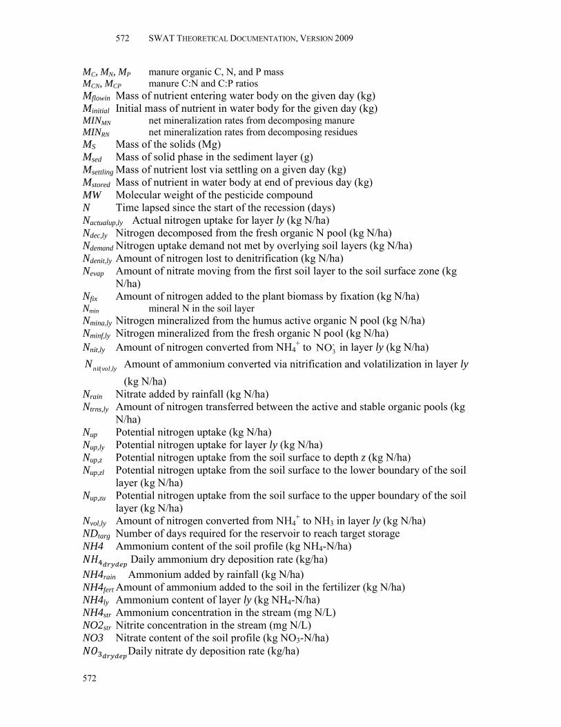
572 SWAT THEORETICAL DOCUMENTATION, VERSION 2009
572
MC, MN, MP manure organic C, N, and P mass MCN, MCP manure C:N and C:P ratios Mflowin Mass of nutrient entering water body on the given day (kg) Minitial Initial mass of nutrient in water body for the given day (kg) MINMN net mineralization rates from decomposing manure MINRN net mineralization rates from decomposing residues MS Mass of the solids (Mg) Msed Mass of solid phase in the sediment layer (g) Msettling Mass of nutrient lost via settling on a given day (kg) Mstored Mass of nutrient in water body at end of previous day (kg) MW Molecular weight of the pesticide compound
N Time lapsed since the start of the recession (days) Nactualup,ly Actual nitrogen uptake for layer ly (kg N/ha) Ndec,ly Nitrogen decomposed from the fresh organic N pool (kg N/ha) Ndemand Nitrogen uptake demand not met by overlying soil layers (kg N/ha) Ndenit,ly Amount of nitrogen lost to denitrification (kg N/ha) Nevap Amount of nitrate moving from the first soil layer to the soil surface zone (kg
N/ha) Nfix Amount of nitrogen added to the plant biomass by fixation (kg N/ha) Nmin mineral N in the soil layer Nmina,ly Nitrogen mineralized from the humus active organic N pool (kg N/ha) Nminf,ly Nitrogen mineralized from the fresh organic N pool (kg N/ha) Nnit,ly Amount of nitrogen converted from NH4
+ to -3NO in layer ly (kg N/ha)
lyvolnitN , Amount of ammonium converted via nitrification and volatilization in layer ly
(kg N/ha) Nrain Nitrate added by rainfall (kg N/ha) Ntrns,ly Amount of nitrogen transferred between the active and stable organic pools (kg
N/ha) Nup Potential nitrogen uptake (kg N/ha) Nup,ly Potential nitrogen uptake for layer ly (kg N/ha) Nup,z Potential nitrogen uptake from the soil surface to depth z (kg N/ha) Nup,zl Potential nitrogen uptake from the soil surface to the lower boundary of the soil
layer (kg N/ha) Nup,zu Potential nitrogen uptake from the soil surface to the upper boundary of the soil
layer (kg N/ha) Nvol,ly Amount of nitrogen converted from NH4
+ to NH3 in layer ly (kg N/ha) NDtarg Number of days required for the reservoir to reach target storage
NH4 Ammonium content of the soil profile (kg NH4-N/ha) Daily ammonium dry deposition rate (kg/ha) NH4rain Ammonium added by rainfall (kg N/ha) NH4fert Amount of ammonium added to the soil in the fertilizer (kg N/ha) NH4ly Ammonium content of layer ly (kg NH4-N/ha) NH4str Ammonium concentration in the stream (mg N/L) NO2str Nitrite concentration in the stream (mg N/L) NO3 Nitrate content of the soil profile (kg NO3-N/ha) Daily nitrate dy deposition rate (kg/ha)
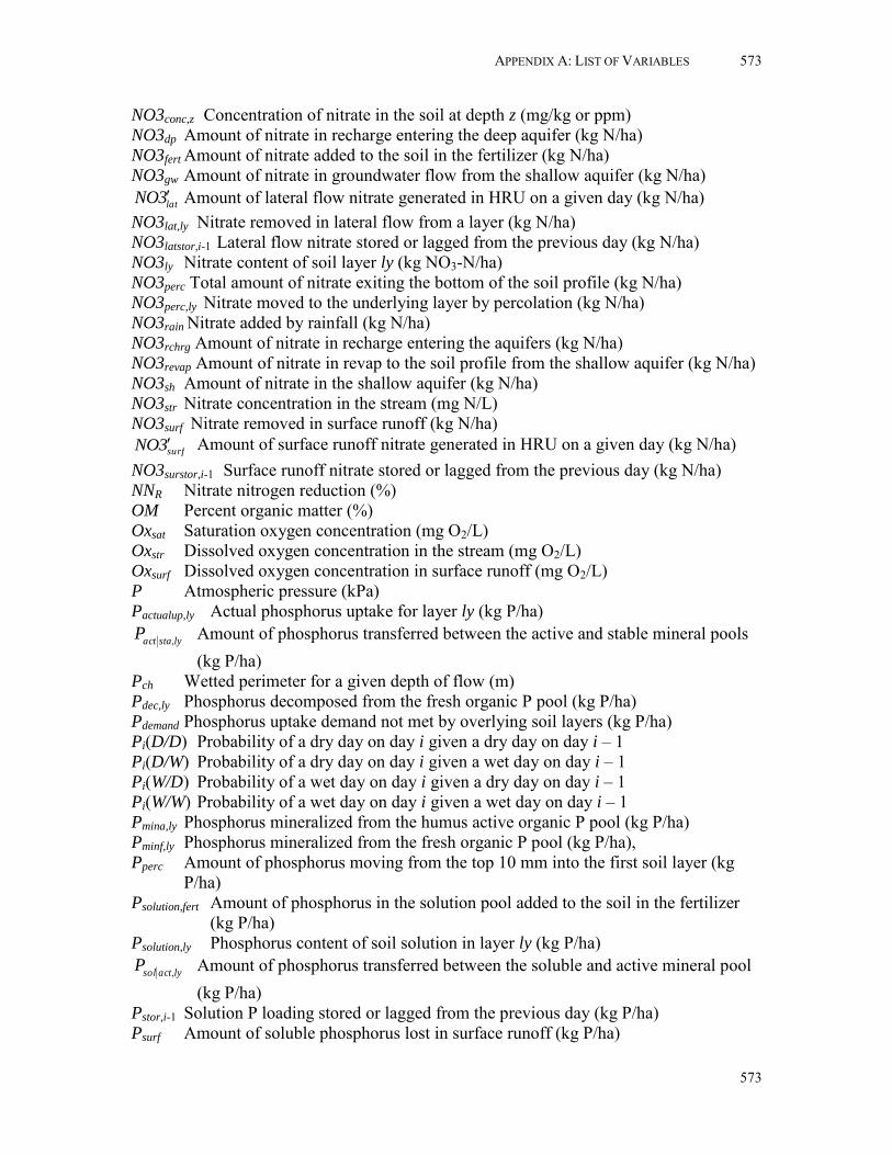
APPENDIX A: LIST OF VARIABLES 573
573
NO3conc,z Concentration of nitrate in the soil at depth z (mg/kg or ppm) NO3dp Amount of nitrate in recharge entering the deep aquifer (kg N/ha) NO3fert Amount of nitrate added to the soil in the fertilizer (kg N/ha) NO3gw Amount of nitrate in groundwater flow from the shallow aquifer (kg N/ha)
lat3NO Amount of lateral flow nitrate generated in HRU on a given day (kg N/ha) NO3lat,ly Nitrate removed in lateral flow from a layer (kg N/ha) NO3latstor,i-1 Lateral flow nitrate stored or lagged from the previous day (kg N/ha) NO3ly Nitrate content of soil layer ly (kg NO3-N/ha) NO3perc Total amount of nitrate exiting the bottom of the soil profile (kg N/ha) NO3perc,ly Nitrate moved to the underlying layer by percolation (kg N/ha) NO3rain Nitrate added by rainfall (kg N/ha) NO3rchrg Amount of nitrate in recharge entering the aquifers (kg N/ha) NO3revap Amount of nitrate in revap to the soil profile from the shallow aquifer (kg N/ha) NO3sh Amount of nitrate in the shallow aquifer (kg N/ha) NO3str Nitrate concentration in the stream (mg N/L) NO3surf Nitrate removed in surface runoff (kg N/ha)
surf3NO Amount of surface runoff nitrate generated in HRU on a given day (kg N/ha) NO3surstor,i-1 Surface runoff nitrate stored or lagged from the previous day (kg N/ha) NNR Nitrate nitrogen reduction (%) OM Percent organic matter (%) Oxsat Saturation oxygen concentration (mg O2/L) Oxstr Dissolved oxygen concentration in the stream (mg O2/L) Oxsurf Dissolved oxygen concentration in surface runoff (mg O2/L) P Atmospheric pressure (kPa) Pactualup,ly Actual phosphorus uptake for layer ly (kg P/ha)
lystaactP , Amount of phosphorus transferred between the active and stable mineral pools
(kg P/ha) Pch Wetted perimeter for a given depth of flow (m) Pdec,ly Phosphorus decomposed from the fresh organic P pool (kg P/ha) Pdemand Phosphorus uptake demand not met by overlying soil layers (kg P/ha) Pi(D/D) Probability of a dry day on day i given a dry day on day i – 1 Pi(D/W) Probability of a dry day on day i given a wet day on day i – 1 Pi(W/D) Probability of a wet day on day i given a dry day on day i – 1 Pi(W/W) Probability of a wet day on day i given a wet day on day i – 1 Pmina,ly Phosphorus mineralized from the humus active organic P pool (kg P/ha) Pminf,ly Phosphorus mineralized from the fresh organic P pool (kg P/ha), Pperc Amount of phosphorus moving from the top 10 mm into the first soil layer (kg
P/ha) Psolution,fert Amount of phosphorus in the solution pool added to the soil in the fertilizer
(kg P/ha) Psolution,ly Phosphorus content of soil solution in layer ly (kg P/ha)
lyactsolP , Amount of phosphorus transferred between the soluble and active mineral pool
(kg P/ha) Pstor,i-1 Solution P loading stored or lagged from the previous day (kg P/ha) Psurf Amount of soluble phosphorus lost in surface runoff (kg P/ha)

574 SWAT THEORETICAL DOCUMENTATION, VERSION 2009
574
surfP Amount of solution P loading generated in HRU on a given day (kg P/ha) Pup Potential phosphorus uptake (kg P/ha) Pup,ly Potential phosphorus uptake for layer ly (kg P/ha) Pup,z Potential phosphorus uptake from the soil surface to depth z (kg P/ha) Pup,zl Potential phosphorus uptake from the soil surface to the lower boundary of the
soil layer (kg P/ha) Pup,zu Potential phosphorus uptake from the soil surface to the upper boundary of the
soil layer (kg P/ha) PUSLE USLE support practice factor POR Porosity of the soil profile (mm) PHU Potential heat units or total heat units required for plant maturity where base
temperature is dependant on the plant species (heat units) PHU0 Total base zero heat units or potential base zero heat units (heat units) Q Volumetric flow rate for water exiting water body (m3 H2O/day) Qgw Groundwater flow, or base flow, into the main channel (mm H2O) Qgw,0 Groundwater flow at the start of the recession (mm H2O) Qgw,N Groundwater flow on day N (mm H2O) Qlat Lateral flow; water discharged from the hillslope outlet (mm H2O/day) Qlatstor,i-1 Lateral flow stored or lagged from the previous day (mm H2O) Qstor Surface runoff stored or lagged (mm H2O) Qsurf Surface runoff on a given day (mm H2O) QSTE Flow rate of STE (m3/day) R Universal gas constant (8.206 10-5 atm m3 (K mole)-1) R0.5sm Smoothed maximum half-hour rainfall for a given month (mm H2O) R0.5x Extreme maximum half-hour rainfall for the specified month (mm H2O) Rt Amount of rain falling during the time step (mm H2O) Rband Precipitation falling in the elevation band (mm H2O) RC, RN, RP residue organic C, N, and P mass RCN, RCP residue C:N and C:P ratios Rch Hydraulic radius for a given depth of flow (m) Rday Amount of rainfall on a given day (mm H2O)
dayR Amount of precipitation on a given day before canopy interception is removed (mm H2O)
Rh Average relative humidity for the day RhDmon Average relative humidity of the month on dry days RhLmon Smallest relative humidity value that can be generated on a given day in the
month Rhmon Average relative humidity for the month Rhmon,mean Mean of RhLmon, Rhmon, and RhUmon RhUmon Largest relative humidity value that can be generated on a given day in the month RhWmon Average relative humidity for the month on wet days RINT Amount of free water held in the canopy on a given day (mm H2O) RL Runoff loading (mm) Rmort Amount of mortality of bacteria (kg/ha) RNO3 Concentration of nitrogen in the rain (mg N/L) RR Runoff reduction (%)

APPENDIX A: LIST OF VARIABLES 575
575
Rresp Amount of respiration of bacteria (kg/ha) Rslough Amount of sloughed off bacteria (kg/ha). Rtc Amount of rain falling during the time of concentration (mm H2O) RUE Radiation-use efficiency of the plant (kg/ha(MJ/m2)-1 or 10-1 g/MJ) RUEamb Radiation-use efficiency of the plant at ambient atmospheric CO2 concentration
(kg/ha(MJ/m2)-1 or 10-1 g/MJ) RUEhi Radiation-use efficiency of the plant at the elevated atmospheric CO2
concentration, CO2hi, (kg/ha(MJ/m2)-1 or 10-1 g/MJ) RUEvpd=1 Radiation-use efficiency for the plant at a vapor pressure deficit of 1 kPa
(kg/ha(MJ/m2)-1 or 10-1 g/MJ) S Retention parameter in SCS curve number equation (mm) S3 Retention parameter for the moisture condition III curve number S Mass of solute sorbed per unit dry weight of solid (mg/kg) SC, SN, SP Soil organic carbon C, N, and P mass SCN, SCP Soil organic C:N and C:P ratios Scap Sediment transport capacity in (mg/m3) Spcon Sediment transport coefficient and v is flow velocity in the waterway (m/s) SolR Soluble pollutant removal (%) SD Runoff depth over unsubmerged waterway area in (mm/day) SolK Saturated hydrologic conductivity of the soil surface (mm/hr) SedR Sediment and particulate pollutant removal (%) SedL Sediment load per unit area of unsubmerged waterway in (kg/ha/day). Sfrz Retention parameter adjusted for frozen conditions (mm) SL Sediment loading (kg/m2) Smax Maximum value the retention parameter can achieve on any given day (mm) Sprev Retention parameter in SCS curve number equation from previous day (mm) SR Sediment reduction (%) Sx Reference or saturation soil organic C mass SA Surface area of the water body (m2) SAem Surface area of the reservoir/pond when filled to the emergency spillway (ha) SAmx Surface area of the wetland when filled to the maximum water level (ha) SAnor Surface area of the wetland when filled to the normal water level (ha) SApr Surface area of the reservoir/pond when filled to the principal spillway (ha) SAT Amount of water in the soil profile when completely saturated (mm H2O), SATly Amount of water in the soil layer when completely saturated (mm H2O) SC Storage coefficient for variable storage flow routing
SD Secchi-disk depth (m) SDco User-defined coefficient to adjust predicted secchi-disk depth SED Solid build up (kg/curb km) SEDmx Maximum accumulation of solids possible for the urban land type (kg/curb km) SNDday Standard normal deviate for the day
SNO Water content of snow cover on current day (mm H2O) SNO100 Amount of snow above which there is 100% cover (mm H2O) SNOmlt Amount of snow melt on a given day (mm H2O) SW Amount of water in soil profile (mm H2O) SWly Soil water content of layer ly (mm H2O)
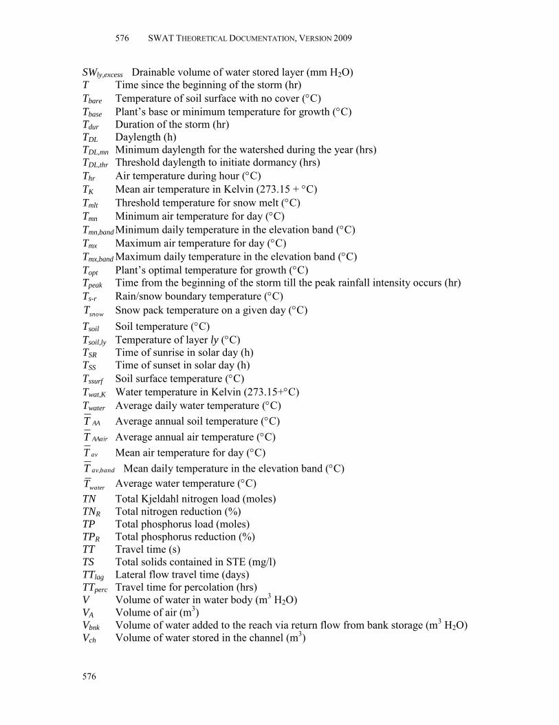
576 SWAT THEORETICAL DOCUMENTATION, VERSION 2009
576
SWly,excess Drainable volume of water stored layer (mm H2O) T Time since the beginning of the storm (hr) Tbare Temperature of soil surface with no cover (C) Tbase Plant’s base or minimum temperature for growth (C) Tdur Duration of the storm (hr) TDL Daylength (h) TDL,mn Minimum daylength for the watershed during the year (hrs) TDL,thr Threshold daylength to initiate dormancy (hrs) Thr Air temperature during hour (C) TK Mean air temperature in Kelvin (273.15 + C) Tmlt Threshold temperature for snow melt (C) Tmn Minimum air temperature for day (C) Tmn,band Minimum daily temperature in the elevation band (C) Tmx Maximum air temperature for day (C) Tmx,band Maximum daily temperature in the elevation band (C) Topt Plant’s optimal temperature for growth (C) Tpeak Time from the beginning of the storm till the peak rainfall intensity occurs (hr) Ts-r Rain/snow boundary temperature (C)
snowT Snow pack temperature on a given day (C) Tsoil Soil temperature (C) Tsoil,ly Temperature of layer ly (C) TSR Time of sunrise in solar day (h) TSS Time of sunset in solar day (h) Tssurf Soil surface temperature (C) Twat,K Water temperature in Kelvin (273.15+C) Twater Average daily water temperature (C)
AAT Average annual soil temperature (C) AAairT Average annual air temperature (C) avT Mean air temperature for day (C)
bandavT , Mean daily temperature in the elevation band (C) waterT Average water temperature (C)
TN Total Kjeldahl nitrogen load (moles) TNR Total nitrogen reduction (%) TP Total phosphorus load (moles) TPR Total phosphorus reduction (%) TT Travel time (s) TS Total solids contained in STE (mg/l) TTlag Lateral flow travel time (days) TTperc Travel time for percolation (hrs) V Volume of water in water body (m3 H2O) VA Volume of air (m3) Vbnk Volume of water added to the reach via return flow from bank storage (m3 H2O) Vch Volume of water stored in the channel (m3)

APPENDIX A: LIST OF VARIABLES 577
577
Vem Volume of water held in the reservoir when filled to the emergency spillway (m3 H2O)
Vevap Volume of water removed from the water body by evaporation during the day (m3 H2O)
Vflowin Volume of water entering water body on given day (m3 H2O) Vflowout Volume of water flowing out of the water body during the day (m3 H2O)
flowoutV Initial estimate of the volume of water flowing out of the water body during the day (m3 H2O)
Vin Volume of inflow during the time step (m3 H2O) Vinitial Initial volume of water in water body on given day (m3 H2O) Vmx Volume of water held in the wetland when filled to the maximum water level (m3
H2O) Vnor Volume of water held in the wetland when filled to the normal water level (m3
H2O) Vout Volume of outflow during the time step (m3 H2O) Vpcp Volume of precipitation falling on the water body during the day (m3 H2O) Vpot,mx Maximum amount of water that can be stored in the pothole (m3 H2O) Vpr Volume of water held in the reservoir when filled to the principal spillway (m3
H2O) VS Volume of solids (m3) Vsed Volume of solids in the sediment layer (m3) Vseep Volume of water lost from the water body by seepage (m3 H2O) Vstored Volume of water stored in water body or channel (m3 H2O) VT Total soil volume (m3) Vtarg Target reservoir volume for a given day (m3 H2O) Vtot Total volume of the sediment layer (m3) VW Volume of water (m3) Vwtr Volume of water in the sediment layer (m3) W Width of channel at water level (m) W(t) Rate of nutrient loading (kg/day) Wbnkfull Top width of the channel when filled with water (m) Wbtm Bottom width of the channel (m) Wbtm,fld Bottom width of the flood plain (m) WP Water content at wilting point (mm H2O) WPly Water content of layer ly at wilting point (mm H2O) X Weighting factor in Muskingum routing
Y Total constituent load (kg) Ysed Cumulative amount of solids washed off at time t (kg/curb km) Zl Soil layer thickness
a Constant in equation used to calculate the cloud cover adjustment factor a1 Constant in equation used to calculate net emissivity
ar Unit channel regression intercept (m3) ax Regression intercept for a channel of length L and width W (m3) aa Exponent between 0 and 1 that varies with atmospheric stability and surface
roughness that is used in calculating wind speed at different heights

578 SWAT THEORETICAL DOCUMENTATION, VERSION 2009
578
adj0.5 Peak rate adjustment factor adjhmd Change in relative humidity expressed as a fraction
adjpcp % change in rainfall adjrad Change in radiation (MJ m-2 d-1) adjtmp Change in temperature (C) algae Algal biomass concentration (mg alg/L) apef Pesticide application efficiency aqdp Amount of water stored in the deep aquifer (mm H2O) aqsh Amount of water stored in the shallow aquifer (mm H2O) aqshthr,q Threshold water level in shallow aquifer for base flow (mm H2O) areahru HRU area (ha or km2) b Constant in equation used to calculate the cloud cover adjustment factor b1 Constant in equation used to calculate net emissivity
bH Scaling factor that controls the degree of deviation in relative humidity caused by the presence or absence of precipitation
bmlt Melt factor for the day (mm H2O/day-C) bmlt6 Melt factor for June 21 (mm H2O/day-C) bmlt12 Melt factor for December 21 (mm H2O/day-C) br Unit channel regression slope
bR Scaling factor that controls the degree of deviation in solar radiation caused by the presence or absence of precipitation
bT Scaling factor that controls the degree of deviation in temperature caused by the presence or absence of precipitation
bx Regression slope for a channel of length L and width W
bactlp,fol Amount of less persistent bacteria attached to the foliage (# cfu/m2) bactlp,perc Amount of less persistent bacteria transported from the top 10 mm into the first
soil layer (#cfu/m2) bactlprch Amount of less persistent bacteria present in the reach (#cfu/100mL) bactlpres Amount of less persistent bacteria present in the reservoir (#cfu/100mL)
sedlptbac , Amount of sediment-attached less persistent bacteria generated in the HRU on a given day (#cfu/m2)
bactlp,sed Amount of less persistent bacteria transported with sediment in surface runoff (#cfu/m2)
bactlp,sedstor,i-1 Sediment-attached less persistent bacteria stored or lagged from the previous day (#cfu/m2)
bactlpsol Amount of less persistent bacteria present in soil solution (#cfu/m2) bactlpsorb Amount of less persistent bacteria in the sorbed pool (# cfu/m2)
surflptbac , Amount of surface runoff less persistent bacteria generated in the HRU on a given day (#cfu/m2)
bactlp,surf Amount of less persistent bacteria lost in surface runoff (#cfu/m2) bactlp,surstor,i-1 Surface runoff less persistent bacteria stored or lagged from the previous
day (#cfu/m2) bactlp,wsh Amount of less persistent bacteria on foliage that is washed off the plant and
onto the soil surface on a given day (# cfu/m2) bactmin Minimum daily loss of bacteria (#cfu/m2)

APPENDIX A: LIST OF VARIABLES 579
579
bactp,fol Amount of persistent bacteria attached to the foliage (# cfu/m2) bactp,perc Amount of persistent bacteria transported from the top 10 mm into the first soil
layer (#cfu/m2) bactprch Amount of persistent bacteria present in the reach (#cfu/100mL) bactpres Amount of persistent bacteria present in the reservoir (#cfu/100mL)
sedptbac , Amount of sediment-attached persistent bacteria generated in the HRU on a given day (#cfu/m2)
bactp,sed Amount of persistent bacteria transported with sediment in surface runoff (#cfu/m2)
bactp,sedstor,i-1 Sediment-attached persistent bacteria stored or lagged from the previous day (#cfu/m2)
bactpsol Amount of persistent bacteria in the solution pool (# cfu/m2) bactpsorb Amount of persistent bacteria in the sorbed pool (# cfu/m2)
surfptbac , Amount of surface runoff persistent bacteria generated in the HRU on a given day (#cfu/m2)
bactp,surf Amount of persistent bacteria lost in surface runoff (#cfu/m2) bactp,surstor,i-1 Surface runoff persistent bacteria stored or lagged from the previous day
(#cfu/m2) bactp,wsh Amount of persistent bacteria on foliage that is washed off the plant and onto the
soil surface on a given day (# cfu/m2) bcv Weighting factor for impact of ground cover on soil surface temperature bio Total plant biomass on a given day (kg/ha) bioag Aboveground biomass on the day of harvest (kg ha-1) bioannual The amount of biomass a tree can accumulate in a single year (kg/ha) biofulldev The biomass of a fully developed tree stand for the specific tree species (metric
tons/ha) bioN Actual mass of nitrogen stored in plant material (kg N/ha) bioN,opt Optimal mass of nitrogen stored in plant material for the growth stage (kg N/ha) bioP Actual mass of phosphorus stored in plant material (kg P/ha) bioP,opt Optimal mass of phosphorus stored in plant material for the current growth stage
(kg P/ha) biotrg Target biomass specified by the user (kg/ha) bnk Total amount of water in bank storage (m3 H2O) bnkin Amount of water entering bank storage (m3 H2O) bnkrevap,mx Maximum amount of water moving into the unsaturated zone in response to
water deficiencies (m3 H2O) c Concentration of nutrient in the water (kg/m3 H2O) ck Celerity corresponding to the flow for a specified depth (m/s) cp Specific heat of moist air at constant pressure (1.013 10-3 MJ kg-1 C-1) cperm Profile-permeability class
csoilstr Soil-structure code used in soil classification csp Coefficient in sediment transport equation canday Maximum amount of water that can be trapped in the canopy on a given day (mm
H2O) canmx Maximum amount of water that can be trapped in the canopy when the canopy is
fully developed (mm H2O)

580 SWAT THEORETICAL DOCUMENTATION, VERSION 2009
580
cbod Carbonaceous biological oxygen demand concentration (mg CBOD/L) cbodsurq CBOD concentration in surface runoff (mg CBOD/L) chla Chlorophyll a concentration (μg chla/L) cncoef Weighting coefficient used to calculate the retention coefficient for daily curve
number calculations dependent on plant evapotranspiration coef1 Weighting coefficient for storage time constant calculation coef2 Weighting coefficient for storage time constant calculation
coefa Empirical water quality factor coefb Empirical dam aeration coefficient coefcrk Adjustment coefficient for crack flow
coefev Evaporation coefficient concN Concentration of nitrogen in a layer (mg/kg or ppm) concNO3,mobile Concentration of nitrate in the mobile water for a given layer (kg N/mm
H2O) concorgN Concentration of organic nitrogen in the soil surface top 10 mm (g N/ metric ton
soil) concP Concentration of phosphorus in a layer (mg/kg or ppm) concpst,flow Concentration of pesticide in the mobile water (kg pst/ha-mm H2O) concsed Concentration of sediment in lateral and groundwater flow (mg/L)
*sedconc “Concentration” of solid particles in the sediment layer (g/m3)
concsed,ch,i Initial sediment concentration in the reach (kg/L or ton/m3) concsed,ch,mx Maximum concentration of sediment that can be transported by the water
(kg/L or ton/m3) concsed,eq Equilibrium concentration of suspended solids in the water body (Mg/m3) concsedlpbact Concentration of less persistent bacteria attached to sediment in the top 10
mm (# cfu/ metric ton soil) concsedpbact Concentration of persistent bacteria attached to sediment in the top 10 mm (#
cfu/ metric ton soil) concsed,surq Concentration of sediment in surface runoff (Mg sed/m3 H2O) concsedP Concentration of phosphorus attached to sediment in the top 10 mm (g P/ metric
ton soil) cov1 Snow cover areal depletion curve shape coefficient cov2 Snow cover areal depletion curve shape coefficient covsol Soil cover index crk Total crack volume for the soil profile on a given day (mm) crkly Crack volume for the soil layer on a given day expressed as a depth (mm) crkly,d-1 Crack volume for the soil layer on the previous day (mm) crkly,i Initial crack volume calculated for the soil layer on a given day expressed as a
depth (mm) crkmax Potential crack volume for the soil profile expressed as a fraction of the total
volume crkmax,ly Maximum crack volume possible for the soil layer (mm) d Zero plane displacement of the wind profile (cm) d1 Equation coefficient for normalized rainfall intensity distribution before peak
intensity is reached

APPENDIX A: LIST OF VARIABLES 581
581
d2 Equation coefficient for normalized rainfall intensity distribution after peak intensity is reached
d50 Median particle size of the inflow sediment (µm) dn Day number of year, 1 on January 1 and 365 on December 31 daysdry Number of dry days in the month dayspcp,yr Average number of days of precipitation in the subbasin in a year daystot Total number of days in the month dayswet Number of wet days in the month dd Damping depth (mm) ddmax Maximum damping depth (mm) depth Depth of water in the channel (m) depthbnkfull Depth of water in the channel when filled to the top of the bank (m) depthdcut Amount of downcutting (m) depthdiff Distance from the bottom of the soil profile to the impervious layer (m) depthfld Depth of water in the flood plain (m) depthimp Depth to the impervious layer (mm) depthly Depth of the soil layer (mm) df Depth factor used in soil temperature calculations div Volume of water added or removed from the reach for the day through diversions
(m3 H2O) dt Length of time step (1 day) durflw Duration of flow (hr) e Actual vapor pressure on a given day (kPa) emon Actual vapor pressure at the mean monthly temperature (kPa)
oe Saturation vapor pressure on a given day (kPa) o
mone Saturation vapor pressure at the mean monthly temperature (kPa) epco Plant uptake compensation factor esco Soil evaporation compensation coefficient expsa Exponent for impoundment surface area calculation
f Coefficient fcl-si Factor that gives low soil erodibility factors for soils with high clay to silt ratios fcld Factor to adjust for cloud cover in net long-wave radiation calculation
fcm Cumulative fmix fcsand Factor that gives low soil erodibility factors for soils with high coarse-sand
contents and high values for soils with little sand fE Combined effect of soil temperature, moisture, and aeration on soil organic
matter, residue, and manure decomposition fgr Growth stage factor in nitrogen fixation equation fhisand Factor that reduces soil erodibility for soils with extremely high sand contents
finf Infiltration rate (mm/hr) fmix Mixing coefficient associated to different tillage tools fNH4 Preference factor for ammonia nitrogen
fno3 Soil nitrate factor in nitrogen fixation equation
fO Aeration factor controlling soil organic matter, residue, and manure decomposition
forgc Factor that reduces soil erodibility for soils with high organic carbon content

582 SWAT THEORETICAL DOCUMENTATION, VERSION 2009
582
fsw Soil water factor in nitrogen fixation equation fT Temperature factor controlling soil organic matter, residue, and manure
decomposition ftool Tillage factor controlling soil organic matter decomposition rate fW Moisture factor controlling soil organic matter, residue, and manure
decomposition fert Amount of fertilizer applied (kg/ha) ferteff Fertilizer application efficiency assigned by the user fertlpbact Concentration of less persistent bacteria in the fertilizer (# cfu/g manure) fertminN Fraction of mineral nitrogen in the fertilizer fertminP Fraction of mineral P in the fertilizer fertNH4 Fraction of mineral N in the fertilizer that is ammonium fertorgN Fraction of organic N in the fertilizer fertorgP Fraction of organic P in the fertilizer fertpbact Concentration of persistent bacteria in the fertilizer (# cfu/g manure) fractive Fraction of the manure containing active colony forming units
fractN Fraction of humic nitrogen in the active pool frav Fraction of the curb length available for sweeping (the availability factor) frbnd Fraction of subbasin area within the elevation band frDL Fraction of daylight hours
frg,mx Fraction of the maximum stomatal conductance, mxg , , achieved at the vapor
pressure deficit, vpdfr frimp Fraction of the subbasin area draining into the impoundment frLAI,1 Fraction of the maximum plant leaf area index corresponding to the 1st point on
the optimal leaf area development curve
frLAI,2 Fraction of the maximum plant leaf area index corresponding to the 2nd point on the optimal leaf area development curve
frLAImx Fraction of the plant’s maximum leaf area index corresponding to a given fraction of potential heat units for the plant
frN Optimal fraction of nitrogen in the plant biomass for current growth stage frN,1 Normal fraction of nitrogen in the plant biomass at emergence frN,2 Normal fraction of nitrogen in the plant biomass at 50% maturity frN,3 Normal fraction of nitrogen in the plant biomass at maturity
frN,~3 Normal fraction of nitrogen in the plant biomass near maturity
frN,yld Fraction of nitrogen in the yield frNH4 Fraction of algal nitrogen uptake from ammonium pool, frnit,ly Estimated fraction of nitrogen lost by nitrification frP Fraction of phosphorus in the plant biomass frP,1 Normal fraction of phosphorus in the plant biomass at emergence frP,2 Normal fraction of phosphorus in the plant biomass at 50% maturity frP,3 Normal fraction of phosphorus in the plant biomass at maturity
frP,~3 Normal fraction of phosphorus in the plant biomass near maturity frP,yld Fraction of phosphorus in the yield
frphosyn Fraction of solar radiation that is photosynthetically active frPHU Fraction of potential heat units accumulated for the plant on a given day in the
growing season

APPENDIX A: LIST OF VARIABLES 583
583
frPHU,1 Fraction of the growing season corresponding to the 1st point on the optimal leaf area development curve
frPHU,2 Fraction of the growing season corresponding to the 2nd point on the optimal leaf area development curve
frPHU,50% Fraction of potential heat units accumulated for the plant at 50% maturity (frPHU,50%=0.5)
frPHU,100% Fraction of potential heat units accumulated for the plant at maturity (frPHU,100%=1.0)
frPHU,sen Fraction of growing season at which senescence becomes the dominant growth process
frpot Fraction of the HRU area draining into the pothole
frroot Fraction of total biomass in the roots on a given day in the growing season
frtrns Fraction of transmission losses partitioned to the deep aquifer frvol,ly Estimated fraction of nitrogen lost by volatilization
frwsh Wash-off fraction for the pesticide frwsh,lp Wash-off fraction for the less persistent bacteria frwsh,p Wash-off fraction for the persistent bacteria frt Fraction of the time step in which water is flowing in the channel g Exponent
g Leaf conductance (m s-1)
mxg , Maximum conductance of a single leaf (m s-1) gmon Skew coefficient for daily precipitation in the month gc Fraction of the ground surface covered by plants hc Canopy height (cm) hc,mx Plant’s maximum canopy height (m) hdrain Height of the tile drain above the impervious zone (mm) hfall Height through which water falls (m) hwtbl Water table height (m) harveff Efficiency of the harvest operation
hr Hour of day (1-24) hR, hM Humification coefficient of residue and manure i Rainfall intensity (mm/hr) imx Maximum rainfall intensity (mm/hr) impcon Fraction of the HRU area that is impervious and hydraulically connected to the
drainage system impdcon Fraction of the HRU area that is impervious but not hydraulically connected to the
drainage system
imptot Fraction of the HRU area that is impervious (both connected and disconnected) irr Amount of irrigation water added on a given day (m3 H2O) IRC, IMCInput of organic C through residue and manure
i Normalized rainfall intensity at time t
i mx Normalized maximum or peak rainfall intensity during the storm
k Von Kármán constant kbact Bacterial partition coefficient kbact,perc Bacteria percolation coefficient (10 m3/Mg)

584 SWAT THEORETICAL DOCUMENTATION, VERSION 2009
584
kbact,surf Bacteria soil partitioning coefficient (m3/Mg) kd,perc Phosphorus percolation coefficient (10 m3/Mg) kd,surf Phosphorus soil partitioning coefficient (m3/Mg) ki Decay constant for rainfall intensity (hr)
k Light extinction coefficient
0,k Non-algal portion of the light extinction coefficient (m-1)
1,k Linear algal self shading coefficient (m-1 (μg-chla/L)-1)
2,k Nonlinear algal self shading coefficient (m-1 (μg-chla/L)-2/3) kM Optimum manure decomposition rate kNO3,sh Rate constant for removal of nitrate in the shallow aquifer (1/day) kp,aq Rate constant for degradation or removal of pesticide in the water (1/day) kp,foliar Rate constant for degradation or removal of the pesticide on foliage (1/day) kp,sed Rate constant for degradation or removal of pesticide in the sediment (1/day) kp,soil Rate constant for degradation or removal of the pesticide in soil (1/day) kr Decay factor (m-1 km-1) ks Sediment settling decay constant (1/day) kx Maximum apparent soil organic matter decomposition rate kk Coefficient in urban wash off equation
m Exponential term in USLE LS factor calculation mc Percent clay content ms Percent sand content msilt Percent silt content (0.002-0.05 mm diameter particles) mvfs Percent very fine sand content (0.05-0.10 mm diameter particles) minNapp Amount of mineral nitrogen applied (kg N/ha) minNapp,mx Maximum amount of mineral N allowed to be applied on any one day (kg
N/ha) minNapp,mxyr Maximum amount of mineral N allowed to be applied during a year (kg
N/ha) minPact,ly Amount of phosphorus in the active mineral pool (mg/kg or kg P/ha) minPsta,ly Amount of phosphorus in the stable mineral pool (mg/kg or kg P/ha) mon Month of the year monfld,beg Beginning month of the flood season monfld,end Ending month of the flood season
n Manning’s roughness coefficient for the subbasin or channel n1 First shape coefficient in plant nitrogen equation n2 Second shape coefficient in plant nitrogen equation
nstrs Nitrogen stress for a given day
orgCly Amount of organic carbon in the layer (%) orgCsurq Organic carbon in surface runoff (kg orgC), orgNact,fert Amount of nitrogen in the active organic pool added to the soil in the fertilizer
(kg N/ha) orgNact,ly Nitrogen in the active organic pool (mg/kg or kg N/ha) orgNfrsh,fert Amount of nitrogen in the fresh organic pool added to the soil in the fertilizer
(kg N/ha) orgNfrsh,surf Nitrogen in the fresh organic pool in the top 10mm (kg N/ha)

APPENDIX A: LIST OF VARIABLES 585
585
orgNhum,ly Humic organic nitrogen in the layer (mg/kg or kg N/ha) orgNsta,ly Nitrogen in the stable organic pool (mg/kg or kg N/ha) orgNstor,i-1 Surface runoff organic N stored or lagged from the previous day (kg N/ha) orgNstr Organic nitrogen concentration in the stream (mg N/L) orgNsurf Amount of organic nitrogen transport to the main channel in surface runoff (kg
N/ha) surfNorg Amount of surface runoff organic N generated in HRU on a given day (kg
N/ha) orgPact,ly Amount of phosphorus in the active organic pool (kg P/ha) orgPfrsh,fert Amount of phosphorus in the fresh organic pool added to the soil in the
fertilizer (kg P/ha) orgPfrsh,ly Phosphorus in the fresh organic pool in layer ly (kg P/ha) orgPhum,fert Amount of phosphorus in the humus organic pool added to the soil in the
fertilizer (kg P/ha) orgPhum,ly Amount of phosphorus in humic organic pool in the layer (mg/kg or kg P/ha) orgPsta,ly Amount of phosphorus in the stable organic pool (kg P/ha) orgPstr Organic phosphorus concentration in the stream (mg P/L) p Total phosphorus concentration (g P/L) p1 First shape coefficient in plant phosphorus equation p2 Second shape coefficient in plant phosphorus equation
pai Phosphorus availability index
pest Actual amount of pesticide applied (kg pst/ha) tpes Effective amount of pesticide applied (kg pst/ha)
pestfol Amount of pesticide applied to foliage (kg pst/ha) pestsurf Amount of pesticide applied to the soil surface (kg pst/ha) plaps Precipitation lapse rate (mm H2O/km) plaque Amount of dead bacteria biomass and residue (kg/ha) prf Peak rate adjustment factor pstbur Amount of pesticide removed via burial (mg pst) pstdeg,sed Amount of pesticide removed from the sediment via degradation (mg pst) pstdeg,wtr Amount of pesticide removed from the water via degradation (mg pst) pstdif Amount of pesticide transferred between the water and sediment by diffusion (mg
pst) pstf Amount of pesticide on the foliage (kg pst/ha) pstf,wsh Amount of pesticide on foliage that is washed off the plant and onto the soil
surface on a given day (kg pst/ha) pstflow Amount of pesticide removed in the flow (kg pst/ha) pstin Pesticide added to the water body via inflow (mg pst)
lattps Amount of lateral flow soluble pesticide generated in HRU on a given day (kg pst/ha)
pstlat,ly Pesticide removed in lateral flow from a layer (kg pst/ha) pstlatstor,i-1 Lateral flow pesticide stored or lagged from the previous day (kg pst/ha) pstlksed Amount of pesticide in the sediment (mg pst) pstlkwtr Amount of pesticide in the water (mg pst) pstperc,ly Pesticide moved to the underlying layer by percolation (kg pst/ha) pstrchsed Amount of pesticide in the sediment (mg pst)

586 SWAT THEORETICAL DOCUMENTATION, VERSION 2009
586
pstrchwtr Amount of pesticide in the water (mg pst) pstrsp,wtr Amount of pesticide removed from sediment via resuspension (mg pst) psts,ly Amount of pesticide in the soil (kg pst/ha) pstsed Amount of sorbed pesticide transported to the main channel in surface runoff (kg
pst/ha) sedtps Sorbed pesticide loading generated in HRU on a given day (kg pst/ha)
pstsedstor,i-1 Sorbed pesticide stored or lagged from the previous day (kg pst/ha) pstsol Solubility of the pesticide in water (mg/L) pstsol,o Amount of dissolved pesticide removed via outflow (mg pst) pstsorb,o Amount of particulate pesticide removed via outflow (mg pst) pststl,wtr Amount of pesticide removed from the water due to settling (mg pst) pstsurf Pesticide removed in surface runoff (kg pst/ha)
surftps Amount of surface runoff soluble pesticide generated in HRU on a given day (kg pst/ha)
pstsurstor,i-1 Surface runoff soluble pesticide stored or lagged from the previous day (kg pst/ha)
pstvol,wtr Amount of pesticide removed via volatilization (mg pst) pstrs Phosphorus stress for a given day
*0q Unit source area flow rate (mm hr-1)
qch Average channel flow rate (m3 s-1) *chq Average channel flow rate (mm hr-1)
qch,pk Peak flow rate (m3/s) qin Inflow rate (m3/s) qout Outflow rate (m3/s) qov Average overland flow rate (m3 s-1) qpeak Peak runoff rate (m3/s or mm/hr) qpeak,f Peak rate after transmission losses (m3/s) qpeak,i Peak rate before accounting for transmission losses (m3/s) qrel Average daily principal spillway release rate (m3/s) qrel,mn Minimum average daily outflow for the month (m3/s) qrel,mx Maximum average daily outflow for the month (m3/s) qtile Average daily tile flow rate (m3/s) r Actual earth-sun distance (AU) r0 Mean earth-sun distance, 1 AU r1 First shape coefficient for radiation-use efficiency curve r2 Second shape coefficient for radiation-use efficiency curve ra Diffusion resistance of the air layer (aerodynamic resistance) (s m-1) rc Plant canopy resistance (s m-1) rg Gaseous surface renewal rate (1/day) rl Liquid surface renewal rate (1/day) r Minimum effective resistance of a single leaf (s m-1)
abr Minimum abaxial stomatal leaf resistance (s m-1)
adr Minimum adaxial stomatal leaf resistance (s m-1) ratioWD Channel width to depth ratio

APPENDIX A: LIST OF VARIABLES 587
587
reff Removal efficiency of the sweeping equipment rexp Exponent for exponential precipitation distribution rnd1 Random number between 0.0 and 1.0 rnd2 Random number between 0.0 and 1.0 rock Percent rock in soil layer (%) rsdly Residue in layer ly (kg/ha) rsdsurf Material in the residue pool for the top 10mm of soil on day i (kg ha-1) sed Sediment yield on a given day (metric tons) sedch Amount of suspended sediment in the reach (metric tons) seddeg Amount of sediment reentrained in the reach segment (metric tons) seddep Amount of sediment deposited in the reach segment (metric tons) sedflowin Amount of sediment added to the water body with inflow (metric tons) sedflowout Amount of sediment transported out of the water body (metric tons) sedlat Sediment loading in lateral and groundwater flow (metric tons) sedout Amount of sediment transported out of the reach (metric tons) sedstl Amount of sediment removed from the water by settling (metric tons) sedstor,i-1 Sediment stored or lagged from the previous day (metric tons) sedwb Sediment in the water body (metric tons) sedPstor,i-1 Sediment-attached P stored or lagged from the previous day (kg P/ha) sedPsurf Amount of phosphorus transported with sediment to the main channel in surface
runoff (kg P/ha) surfPsed Amount of sediment-attached P loading generated in HRU on a given day (kg
P/ha) slp Average slope of the subbasin (% or m/m) slpch Average channel slope along channel length (m m-1) snocov Fraction of the HRU area covered by snow spexp Exponent in sediment transport equation
starg Target reservoir volume specified for a given month (m3 H2O) surlag Surface runoff lag coefficient t Number of hours before (+) or after (-) solar noon t1/2,aq Aqueous half-life for the pesticide (days) t1/2,f Half-life of the pesticide on foliage (days) t1/2,NO3,sh Half-life of nitrate in the shallow aquifer (days) t1/2,s Half-life of the pesticide in the soil (days) t1/2,sed Sediment half-life for the pesticide (days) thalf Length of time needed for solid build up to increase from 0 kg/curb km to ½
SEDmx (days) tch Time of concentration for channel flow (hr) tconc Time of concentration for a subbasin (hr) tdorm Dormancy threshold (hrs) tdrain Time required to drain the soil to field capacity (hrs) ti Solar time at the midpoint of the hour i tov Time of concentration for overland flow (hr) tilelag Drain tile lag time (hrs). tilewtr Amount of water removed from the layer on a given day by tile drainage (mm
H2O)

588 SWAT THEORETICAL DOCUMENTATION, VERSION 2009
588
tlaps Temperature lapse rate (C/km) tloss Channel transmission losses (m3 H2O) trapef Fraction of the constituent loading trapped by the filter strip
trapef,bact Fraction of the bacteria loading trapped by the filter strip trapef,sub Fraction of the subsurface flow constituent loading trapped by the filter strip
tstrs Temperature stress for a given day expressed as a fraction of optimal plant growth
t Time during the storm expressed as a fraction of the total storm duration (0.0-1.0) t peak Time from the beginning of the storm till the peak intensity expressed as a
fraction of the total storm duration (0.0-1.0) meanpeakt ,
ˆ Mean of peakLt , peakMt , and peakUt
peakLt Minimum time to peak intensity that can be generated
peakMt Average time to peak intensity expressed as a fraction of storm duration
peakUt Maximum time to peak intensity that can be generated
uz Wind speed at height zw (m s-1) uz1 Wind speed (m s-1) at height z1
uz2 Wind speed (m s-1) at height z2
urbcoef Wash off coefficient (mm-1) vb Pesticide burial velocity (m/day) vc Average channel velocity (m s-1) vch,pk Peak channel velocity (m/s) vd Pesticide rate of diffusion or mixing velocity (m/day) vlat Velocity of flow at the hillslope outlet (mm∙h-1) vov Overland flow velocity (m s-1) vp Pore velocity in the biozone layer (mm/day) vr Pesticide resuspension velocity (m/day) vs Pesticide settling velocity (m/day) vsurf Surface runoff flow rate (m3/s) vv Pesticide volatilization mass-transfer coefficient (m/day) volQsurf,f Volume of runoff after transmission losses (m3) volQsurf,i Volume of runoff prior to transmission losses (m3) volthr Threshold volume for a channel of length L and width W (m3) vpd Vapor pressure deficit (kPa) vpdfr Vapor pressure deficit corresponding to frg,mx (kPa) vpdthr Threshold vapor pressure deficit above which a plant will exhibit reduced leaf
conductance or reduced radiation-use efficiency (kPa) w1 Shape coefficient in retention parameter adjustments for soil moisture content w2 Shape coefficient in retention parameter adjustments for soil moisture content wactualup Total plant water uptake for the day (mm H2O) wactualup,ly Actual water uptake for layer ly (mm H2O) wcrk,btm Amount of water flow past the lower boundary of the soil profile due to bypass
flow (mm H2O) wdeep Amount of water percolating from the shallow aquifer into the deep aquifer (mm
H2O) wdemand Water uptake demand not met by overlying soil layers (mm H2O)

APPENDIX A: LIST OF VARIABLES 589
589
winf Amount of water entering the soil profile on a given day (mm H2O) wmobile Amount of mobile water in the layer (mm H2O) wperc,ly Amount of water percolating to the underlying soil layer on a given day (mm
H2O) wpump,dp Amount of water removed from the deep aquifer by pumping (mm H2O) wpump,sh Amount of water removed from the shallow aquifer by pumping (mm H2O) wrchrg Amount of water entering the aquifer via recharge (mm H2O) wrchrg,sh Amount of water entering the shallow aquifer via recharge (mm H2O) wrevap Amount of water moving into the soil zone in response to water deficiencies (mm
H2O) wrevap,mx Maximum amount of water moving into the soil zone in response to water
deficiencies on day i (mm H2O) wseep Total amount of water exiting the bottom of the soil profile (mm H2O) wup,ly Potential water uptake for layer ly (mm H2O)
lyupw , Adjusted potential water uptake for layer ly (mm H2O)
lyupw , Potential water uptake when the soil water content is less than 25% of plant available water (mm H2O)
wup,z Potential water uptake from the soil surface to a specified depth, z, on a given day (mm H2O)
wup,zl Potential water uptake for the profile to the lower boundary of the soil layer (mm H2O)
wup,zu Potential water uptake for the profile to the upper boundary of the soil layer (mm H2O)
widthfiltstrip Width of filter strip (m) wstrs Water stress for a given day expressed as a fraction of total water demand yld Crop yield (kg/ha) yldact Actual yield (kg ha-1) yldest,N Nitrogen yield estimate (kg N/ha) yldest,Nprev Nitrogen yield estimate from the previous year (kg N/ha) yldN Amount of nitrogen removed in the yield (kg N/ha) yldP Amount of phosphorus removed in the yield (kg P/ha) yldyr,N Nitrogen yield target for the current year (kg N/ha) yrcur The number of years of development the tree has accrued (years) yrfulldev The number of years for the tree species to reach full development (years) yrsim Year of simulation (1 to yrtot) yrtot Total number of calendar years simulated yrs Number of years of rainfall data used to obtain values for monthly extreme half-
hour rainfalls
z Depth below soil surface (mm) z1 Height of wind speed measurement (cm) z2 Height of wind speed measurement (cm) zch Inverse of the channel side slope
zfld Inverse of the flood plain side slope
zg Thickness of the gas film (m) zl Thickness of the liquid film (m) zl,ly Depth from the surface to the bottom of the soil layer (mm)

590 SWAT THEORETICAL DOCUMENTATION, VERSION 2009
590
zmid,ly Depth from the soil surface to the middle of the layer (mm) zom Roughness length for momentum transfer (cm) zov Roughness length for vapor transfer (cm) zp Height of the humidity (psychrometer) and temperature measurements (cm) zroot Depth of root development in the soil (mm) zroot,mx Maximum depth for root development in the soil (mm) ztot Depth to bottom of soil profile (mm) zw Height of the wind speed measurement (cm) zd Ratio of depth in soil to damping depth Gram of live bacteria growth to gram of BOD in STE (conversion factor) Short-wave reflectance or albedo 0 Ratio of chlorophyll a to algal biomass (μg chla/mg alg) 0.5 Maximum half-hour rainfall expressed as a fraction of daily rainfall 0.5L Smallest half-hour rainfall fraction that can be generated on a given day
0.5mean Mean of 0.5L, 0.5mon, 0.5U 0.5mon Average maximum half-hour rainfall fraction for the month
0.5U Largest half-hour rainfall fraction that can be generated on a given day
1 Fraction of algal biomass that is nitrogen (mg N/mg alg biomass), 2 Fraction of algal biomass that is phosphorus (mg P/mg alg biomass) 3 Rate of oxygen production per unit of algal photosynthesis (mg O2/mg alg) 4 Rate of oxygen uptake per unit of algae respired (mg O2/mg alg) 5 Rate of oxygen uptake per unit NH4
+ oxidation (mg O2/mg N) 6 Rate of oxygen uptake per unit NO2 oxidation (mg O2/mg N) bnk Bank flow recession constant or constant of proportionality
gw Baseflow recession constant hill Slope of the hillslope segment (degrees) pet Coefficient in Priestley-Taylor equation
plant Plant albedo (set at 0.23) soil Soil albedo tc Fraction of daily rainfall that occurs during the time of concentration
0 Coefficient for USGS regression equations for urban loadings 1 Coefficient for USGS regression equations for urban loadings 2 Coefficient for USGS regression equations for urban loadings 3 Coefficient for USGS regression equations for urban loadings 4 Coefficient for USGS regression equations for urban loadings deep Aquifer percolation coefficient denit Rate coefficient for denitrification eqP Slow equilibration rate constant (0.0006 d-1) min Rate coefficient for mineralization of the humus active organic nutrients n Nitrogen uptake distribution parameter N,1 Rate constant for biological oxidation of ammonia nitrogen (day-1 or hr-1) N,1,20 Rate constant for biological oxidation of ammonia nitrogen at 20C (day-1 or hr-1) N,2 Rate constant for biological oxidation of nitrite to nitrate (day-1 or hr-1)

APPENDIX A: LIST OF VARIABLES 591
591
N,2,20 Rate constant for biological oxidation of nitrite to nitrate at 20C (day-1 or hr-1) N,3 Rate constant for hydrolysis of organic nitrogen to ammonia nitrogen (day-1 or hr-1) N,3,20 Local rate constant for hydrolysis of organic nitrogen to NH4
+ at 20C (day-1 or hr-1)
NO3 Nitrate percolation coefficient p Phosphorus uptake distribution parameter P,4 Rate constant for mineralization of organic phosphorus (day-1 or hr-1) P,4,20 Local rate constant for organic phosphorus mineralization at 20C (day-1 or hr-1) pst Pesticide percolation coefficient rev Revap coefficient rsd Rate coefficient for mineralization of the residue fresh organic nutrients sa Coefficient for impoundment surface area equation trns Rate constant for nitrogen transfer between active and stable organic pools (110-5) w Water-use distribution parameter i(j) 3 1 matrix for day i whose elements are residuals of maximum temperature (j =
1), minimum temperature (j = 2) and solar radiation (j = 3), Slope of the saturation vapor pressure curve (kPa C-1) algae Change in algal biomass concentration (mg alg/L) bio Potential increase in total plant biomass on a given day (kg/ha) bioact Actual increase in total plant biomass on a given day (kg/ha)
dclg , Rate of decline in leaf conductance per unit increase in vapor pressure deficit (m s-1 kPa-1)
LAIi Leaf area added on day i (potential) LAIact,i Actual leaf area added on day i NH4str Change in ammonium concentration (mg N/L) NO2str Change in nitrite concentration (mg N/L) orgNstr Change in organic nitrogen concentration (mg N/L) orgPstr Change in organic phosphorus concentration (mg P/L) Oxstr Change in dissolved oxygen concentration (mg O2/L) pstlkwtr Change in pesticide mass in the water layer (mg pst) pstlksed Change in pesticide mass in the sediment layer (mg pst) pstrchwtr Change in pesticide mass in the water layer (mg pst) pstrchsed Change in pesticide mass in the sediment layer (mg pst) rsd Biomass added to the residue pool on a given day (kg ha-1) ruedcl Rate of decline in radiation-use efficiency per unit increase in vapor pressure
deficit (kg/ha(MJ/m2)-1kPa-1 or (10-1 g/MJ)kPa-1)
solPstr Change in solution phosphorus concentration (mg P/L) t Length of the time step (s) δ Solar declination (radians) Exponential coefficient (unitless) 1 Equation coefficient for rainfall intensity before peak intensity is reached (hr) 2 Equation coefficient for rainfall intensity after peak intensity is reached (hr) gw Delay time or drainage time for aquifer recharge (days) ntr,ly Residue decay rate constant

592 SWAT THEORETICAL DOCUMENTATION, VERSION 2009
592
Emissivity Net emittance Field capacity coefficient 2 (unitless). a Atmospheric emittance bact:sed Bacteria enrichment ratio
C:N Residue C:N ratio in the soil layer C:P Residue C:P ratio in the soil layer C:sed Carbon enrichment ratio
i 3 1 matrix of independent random components N:sed Nitrogen enrichment ratio
P:sed Phosphorus enrichment ratio
pst:sed Pesticide enrichment ratio sr Radiation term for bare soil surface temperature calculation vs Vegetative or soil emittance Field capacity coefficient 1 (unitless), Latitude in radians
air Air-filled porosity expressed as a fraction d Drainable porosity of the soil (mm/mm) fc Porosity of the soil layer filled with water when the layer is at field capacity water
content (mm/mm) soil Porosity of the soil (mm/mm) Psychrometric constant (kPa C-1) Respiration rate coefficient (unitless). ntr,ly Nutrient cycling residue composition factor for layer ly reg Plant growth factor (0.0-1.0) sw,ly Nutrient cycling water factor for layer ly sw,thr Threshold value of nutrient cycling water factor for denitrification to occur tmp,ly Nutrient cycling temperature factor for layer ly wu Water deficiency factor Evaporation coefficient (0.6) Linear coefficient (kg/ha cec,ly Volatilization cation exchange capacity factor midz,ly Volatilization depth factor nit,ly Nitrification regulator sw,ly Nitrification soil water factor tmp,ly Nitrification/volatilization temperature factor vol,ly Volatilization regulator Mortality rate coefficient (unitless). Scaling factor for impact of soil water on damping depth n Scaling factor for nitrogen stress equation p Scaling factor for phosphorus stress equation
1 CBOD deoxygenation rate (day-1 or hr-1) 1,20 CBOD deoxygenation rate at 20C (day-1 or hr-1)

APPENDIX A: LIST OF VARIABLES 593
593
2 Reaeration rate for Fickian diffusion (day-1 or hr-1) 2,20 Reaeration rate at 20C (day-1 or hr-1) 3 Settling loss rate of CBOD (day-1 or hr-1) 3,20 Settling loss rate of CBOD at 20C (day-1 or hr-1) 4 Sediment oxygen demand rate (mg O2/(m2
day)) 4,20 Sediment oxygen demand rate at 20C (mg O2/(m2
day) or mg O2/(m2hr))
Latent heat of vaporization (MJ kg-1) Lag coefficient that controls influence of previous day’s temperature on current
day’s temperature 1 First shape coefficient for optimal leaf area development curve
2 Second shape coefficient for optimal leaf area development curve
crk Lag factor for crack development during drying
sno Snow temperature lag factor Specific yield of the shallow aquifer (m/m) 10m Mean wind speed for the day at height of 10 meters (m s-1) a Local specific growth rate of algae (day-1) a,20 Local specific algal growth rate at 20C (day-1 or hr-1) μlpfol,die,20 Rate constant for die-off of less persistent bacteria on foliage at 20C
(1/day) μlpfol,grw,20 Rate constant for re-growth of less persistent bacteria on foliage at 20C
(1/day) μlpfol,net Overall rate constant for die-off/re-growth of less persistent bacteria on
foliage (1/day) μlpfol,net,20 Overall rate constant for die-off/re-growth of less persistent bacteria on
foliage at 20C (1/day) μlprch,die Rate constant for die-off of less persistent bacteria in streams (1/day)
μlprch,die,20 Rate constant for die-off of less persistent bacteria in streams at 20C (1/day) μlpres,die Rate constant for die-off of less persistent bacteria in water bodies (1/day)
μlpres,die,20 Rate constant for die-off of less persistent bacteria in water bodies at 20C (1/day)
μlpsol,die,20 Rate constant for die-off of less persistent bacteria in soil solution at 20C (1/day)
μlpsol,grw,20 Rate constant for re-growth of less persistent bacteria in soil solution at 20C (1/day)
μlpsol,net Overall rate constant for die-off/re-growth of less persistent bacteria in soil solution (1/day)
μlpsol,net,20 Overall rate constant for die-off/re-growth of less persistent bacteria in soil solution at 20C (1/day)
μlpsorb,die,20 Rate constant for die-off of less persistent bacteria attached to soil particles at 20C (1/day)
μlpsorb,grw,20 Rate constant for re-growth of less persistent bacteria attached to soil particles at 20C (1/day)

594 SWAT THEORETICAL DOCUMENTATION, VERSION 2009
594
μlpsorb,net Overall rate constant for die-off/re-growth of less persistent bacteria sorbed to the soil (1/day)
μlpsorb,net,20 Overall rate constant for die-off/re-growth of less persistent bacteria attached to soil particles at 20C (1/day)
max Maximum specific algal growth rate (day-1 or hr-1) mon Mean daily rainfall (mm H2O) for the month μpfol,die,20 Rate constant for die-off of persistent bacteria on foliage at 20C (1/day) μpfol,grw,20 Rate constant for re-growth of persistent bacteria on foliage at 20C
(1/day) μpfol,net Overall rate constant for die-off/re-growth of persistent bacteria on foliage
(1/day) μpfol,net,20 Overall rate constant for die-off/re-growth of persistent bacteria on foliage
at 20C (1/day) μprch,die Rate constant for die-off of persistent bacteria in streams (1/day) μprch,die,20 Rate constant for die-off of persistent bacteria in streams at 20C (1/day) μpres,die Rate constant for die-off of persistent bacteria in water bodies (1/day) μpres,die,20 Rate constant for die-off of persistent bacteria in water bodies at 20C (1/day) μpsol,die,20 Rate constant for die-off of persistent bacteria in soil solution at 20C
(1/day) μpsol,grw,20 Rate constant for re-growth of persistent bacteria in soil solution at 20C
(1/day) μpsol,net Overall rate constant for die-off/re-growth of persistent bacteria in soil solution
(1/day) μpsol,net,20 Overall rate constant for die-off/re-growth of persistent bacteria in soil
solution at 20C (1/day) μpsorb,die,20 Rate constant for die-off of persistent bacteria attached to soil particles at
20C (1/day) μpsorb,grw,20 Rate constant for re-growth of persistent bacteria attached to soil particles
at 20C (1/day) μpsorb,net Overall rate constant for die-off/re-growth of persistent bacteria sorbed to
the soil (1/day) μpsorb,net,20 Overall rate constant for die-off/re-growth of persistent bacteria attached
to soil particles at 20C (1/day) dewmon Average dew point temperature for the month (C) Dmxmon Average daily maximum temperature of the month on dry days (C) Dradmon Average daily solar radiation of the month on dry days (MJ m-2) mnmon Average daily minimum temperature for the month (C) mxmon Average daily maximum temperature for the month (C) radmon Average daily solar radiation for the month (MJ m-2) tmpmon Mean air temperature for the month (C) w Wind speed (m/s) Wmxmon Average daily maximum temperature of the month on wet days (C) wndmon Average wind speed for the month (m s-1) Wradmon Average daily solar radiation of the month on wet days (MJ m-2)

APPENDIX A: LIST OF VARIABLES 595
595
Apparent settling velocity (m/day) Moisture content of biozone (mm) θbact Temperature adjustment factor for bacteria die-off/re-growth
e Fraction of water volume that excludes anions f
t Field capacity at the end of the day (mm) f
t-1 Field capacity at the beginning of the day (mm) s
t-1 Saturated moisture content at the beginning of the day (mm) si Initial soil porosity with zero plaque (mm) v Volumetric moisture content (mm/mm) θz Zenith angle (radians) 0(j,k) Correlation coefficient between variables j and k on the same day where j and k
may be set to 1 (maximum temperature), 2 (minimum temperature) or 3 (solar radiation)
1(j,k) Correlation coefficient between variable j and k with variable k lagged one day with respect to variable j
a Local respiration rate of algae (day-1) a,20 Local algal respiration rate at 20C (day-1 or hr-1) ρair Air density (kg m-3) b Soil bulk density (Mg m-3) bm Density of live bacterial biomass (~1000 kg/m3 ) s Particle density (Mg m-3) w Density of water (1 Mg m-3) alibration parameter to convert total solids in STE to plaque (unitless) Stefan-Boltzmann constant (4.903 10-9 MJ m-2 K-4 d-1) 1 Local settling rate for algae (m/day) 1,20 Local algal settling rate at 20C (m/day or m/hr) 2 Benthos (sediment) source rate for soluble P (mg P/m2-day or mg P/m2-hr) 2,20 Benthos (sediment) source rate for soluble phosphorus at 20C (mg P/m2-day or mg
P/m2-hr) 3 Benthos (sediment) source rate for ammonium (mg N/m2-day or mg N/m2-hr) 3,20 Benthos (sediment) source rate for ammonium nitrogen at 20C (mg N/m2-day or
mg N/m2-hr) 4 Rate coefficient of organic nitrogen settling (day-1 or hr-1) 4,20 Local settling rate for organic nitrogen at 20C (day-1 or hr-1) 5 Rate coefficient for organic phosphorus settling (day-1 or hr-1) 5,20 Local settling rate for organic phosphorus at 20C (day-1 or hr-1) mon Standard deviation of daily rainfall (mm H2O) for the month mnmon Standard deviation for daily minimum temperature during the month (C) mxmon Standard deviation for daily maximum temperature during the month (C) radmon Standard deviation for daily solar radiation during the month (MJ m-2) Angular velocity of the earth's rotation (0.2618 radians h-1) tmp Angular frequency in soil temperature variation wf Wetting front matric potential (mm)

596 SWAT THEORETICAL DOCUMENTATION, VERSION 2009
596

597
APPENDIX B
REFERENCES

598 SWAT THEORETICAL DOCUMENTATION, VERSION 2009
598
Allen, R.G. 1986. A Penman for all seasons. J. Irrig. and Drain Engng., ASCE,
112(4): 348-368.
Allen, P.M., J. Arnold, E. Jakubowski. 1999. Prediction of stream channel erosion
potential. Environmental and Engineering Geoscience 5:339-351.
Allen, R.G., M.E. Jensen, J.L. Wright, and R.D. Burman. 1989. Operational
estimates of evapotranspiration. Agron. J. 81:650-662.
American Public Health Association. 1985. Standard methods for the examination
of water and wastewater, 16th edition. American Public Health
Association, Inc.
American Society for Testing and Materials. 1995. Annual book of ASTM
standards, Vol. 04.08, Designation: D 5852-5. American Society for
Testing and Materials, Philidelphia, PA. p. 653-657.
Anderson, E.A. 1976. A point energy and mass balance model of snow cover.
NOAA Technical Report NWS 19, U.S. Dept. of Commerce, National
Weather Service.
Arabi M, Frankenberger JR, Engel BE, Arnold JG. 2008. Representation of
agricultural conservation practices with SWAT. Hydrological Processes
22(16): 3042-3055.
Arnold, J.G., P.M. Allen, and G. Bernhardt. 1993. A comprehensive surface-
groundwater flow model. J. Hydrol. 142:47-69.
Arnold, J. G., R. Srinivasan, R. S. Muttiah, and J. R. Williams. 1998. Large area
hydrologic modeling and assessment: Part I. Model development. J.
American Water Resources Assoc. 34:73-89.
Arnold, J.G. and J.R. Williams. 1995. SWRRB—A watershed scale model for soil
and water resources management. p. 847-908. In V.P. Singh (ed)
Computer models of watershed hydrology. Water Resources Publications.
Arnold, J.G., J.R. Williams and D.R. Maidment. 1995. Continuous-time water and
sediment-routing model for large basins. Journal of Hydraulic Engineering
121(2):171-183.

APPENDIX B: REFERENCES 599
599
Arnold, J.G., J.R. Williams, A.D. Nicks, and N.B. Sammons. 1990. SWRRB: A
basin scale simulation model for soil and water resources management.
Texas A&M Univ. Press, College Station, TX.
Azevedo, J., and P.R. Stout. 1974. Farm animal manures: An overview of their
role in the agricultural environment (Service Manual no. 44). University of
California, Agricultural Experiment Station Extension.
Bagnold, R.A. 1977. Bedload transport in natural rivers. Water Resources Res.
13(2):303-312.
Barfield BJ, Blevins RL, Fogle AW, Madison CE, Inamdar S, Carey DI,
Evangelou VP. 1998. Water quality impacts of natural filter strips in karst
areas. Transactions of the ASAE 41(2): 371-381.
Barnard, J.D. 1948. Heat units as a measure of canning crop maturity. The Canner
106:28.
Barrow, N.J. and T.C. Shaw. 1975. The slow reactions between soil and anions. 2.
Effect of time and temperature on the decrease in phosphate concentration
in soil solution. Soil Sci. 119:167-177.
Bengston, L. 1981. Snowmelt-generated runoff in urban areas. p. 444-451. In
B.C. Yen (ed.) Urban stormwater hydraulics and hydrology: proceedings
of the Second International Conference on Urban Storm Drainage, held at
Urbana, Illinois, USA, 15-19 June 1981. Water Resources Publications,
Littleton, CO.
Bond, C., Maguire, R., and Havlin, J. (2006). "Change in soluble phosphorus in
soils following fertilization is dependent on initial Mehlich-3 phosphorus."
J. Environ. Qual., 35(5), 1818.
Boswell, V.G. 1926. The influence of temperature upon the growth and yield of
garden peas. Proc. Amer. Soc. Hort. Sci. 23:162-168.
Boswell, V.G. 1929. Factors influencing yield and quality of peas—Biophysical
and biochemical studies. Maryland Agr. Exp. Sta. Bul. 306.
Bouma, J. and J. Loveday. 1988. Chapter 5: Characterizing soil water regimes in
swelling clay soils. p. 83-96. In L.P. Wilding and R. Puentes (ed).
600 SWAT THEORETICAL DOCUMENTATION, VERSION 2009
600
Vertisols: their distribution, properties, classification and management.
Texas A&M University Printing Center, College Station, TX.
Bouwer, H. 1969. Infiltration of water into nonuniform soil. Journal Irrigation and
Drainage Div., ASCE 95(IR4):451-462.
Bowie, G.L. W.B. Mills, D.B. Porcella, C.L. Campbell, J.R. Pagenkopt, G.L.
Rupp, K.M. Johnson, P.W.H. Chan, and S.A. Gherini. 1985. Rates,
constants, and kinetic formulations in surface water quality modeling, 2nd
ed. EPA/600/3-85/040, U.S. Environmental Protection Agency, Athens,
GA.
Bradbury, N.J., A.P. Whitmore, P.B.S. Hart, and D.S. Jenskinson, 1993.
Modelling the fate of nitrogen in crop and soil in the years following
application of 15N-labelled fertilizer to winter wheat. J. Agric. Sci.
121:363-379.
Brakensiek, D.L. 1967. Kinematic flood routing. Transactions of the ASAE
10(3):340-343.
Bronswijk, J.J.B. 1989. Prediction of actual cracking and subsidence in clay soils.
Soil Science 148:87-93.
Bronswijk, J.J.B. 1990. Shrinkage geometry of a heavy clay soil at various
stresses. Soil Science Soc. Am. J. 54:1500-1502.
Brown, L.C. and T.O. Barnwell, Jr. 1987. The enhanced water quality models
QUAL2E and QUAL2E-UNCAS documentation and user manual. EPA
document EPA/600/3-87/007. USEPA, Athens, GA.
Brunt, D. 1932. Notes on radiation in the atmosphere. Quart. J. Roy. Meteorol.
Soc. 58: 389-418.
Brunt, D. 1952. Physical and dynamical meteorology, 2nd ed. University Press,
Cambridge.
Brutsaert, W. 1975. Comments on surface roughness parameters and the height of
dense vegetation. J. Meterol. Soc. Japan 53:96-97.
Bruun, S. and J. Luxhoi, 2006. Letter to the Editor on ―Can incubations be use to
measure meaningful pools of soil organic matter? Soil Sci Soc Am J,
70:2164.

APPENDIX B: REFERENCES 601
601
Bumgarner, J.R., McCray, J.E., 2007. Estimating Biozone Hydraulic Conductivity
in Wastewater Soil-infiltration Systems using Inverse Numerical
modeling. Water Research, 41(11): 2349-2360.
Campbell, G.S. 1985. Soil physics with BASIC: transport models for soil-plant
systems. Elsevier, Amsterdam.
Carslaw, H.S. and J.C. Jaeger. 1959. Conduction of heat in solids. Oxford
University Press, London.
Chapra, S.C. 1997. Surface water-quality modeling. McGraw-Hill, Boston.
Chow, V.T. 1959. Open-channel hydraulics. McGraw-Hill, New York.
Chow, V.T., D.R. Maidment, and L.W. Mays. 1988. Applied hydrology.
McGraw-Hill, Inc., New York, NY.
Chu T, Shirmohammadi A, Abbott L, Sadeghi A, Montas H. 2005. Watershed
level BMP evaluation with SWAT model. In proceedings of the American
Society of Agricultural Engineers Annual International Meeting. July 17-
20, 2005, Tampa, Florida, USA. ASABE Publication number 052098.
Churchill, M.A., H.L. Elmore, and R.A. Buckingham. 1962. The prediction of
stream reaeration rates. International Journal of Air and Water Pollution.
6: 467-504.
Clean Air Status and Trends Network (CASTNET), 2007.
http://www.epa.gov/castnet/docs/CASTNET_factsheet_2007.pdf
Cluis, D., P. Couture, R. Bégin, and S.A. Visser. 1988. Potential eutrophication
assessment in rivers; relationship between produced and exported loads.
Schweiz. Z. Hydrol. 50:166-181.
Collins, H.P., E.T. Elliott, K. Paustian, L.G. Bundy, W.A. Dick, D.R. Huggins,
D.R., A.J.M Smucker, and E.M. Paul, 2000. Soil carbon pools and fluxes
in long-term corn belt agroecosystems. Soil Biol. Biochem. 32:157-163.
Cope, J.T., C.E. Evans, and H.C. Williams. 1981. Soil test fertility
recommendations for Alabama crops. Alabama Agric. Station Circular
No. 251.

602 SWAT THEORETICAL DOCUMENTATION, VERSION 2009
602
Cross, H.Z. and M.S. Zuber. 1972. Prediction of flowering dates in maize based
on different methods of estimating thermal units. Agronomy Journal
64:351-355.
Cunge, J.A. 1969. On the subject of a flood propagation method (Muskingum
method). J. Hydraulics Research 7(2):205-230.
Danckwerts, P.V. 1951. Significance of liquid-film coefficients in gas absorption.
Ind. Eng. Chem. 43:1460-1467.
Dillaha TA, Reneau RB, Mostaghimi S, Lee D. 1989. Vegetative filter strips for
agricultural nonpoint source pollution control. Transactions of the ASAE
32(2): 513-519.
Dingman, S.L. 1994. Physical hydrology. Prentice-Hall, Inc., Englewood Cliffs,
NJ.
Domenico, P.A. and F.W. Schwartz. 1990. Physical and chemical hydrology.
John Wiley & Sons, New York, NY.
Doorenbos, J. and W.O. Pruitt. 1977. Guidelines for predicting crop water
requirements. FAO Irrig. and Drain. Paper No. 24, 2nd ed. FAO, Rome.
Dorioz JM, Wang D, Poulenard J, Trévisan D. 2006. The effect of grass buffer
strips on phosphorus dynamics--A critical review and synthesis as a basis
for application in agricultural landscapes in France. Agriculture,
Ecosystems & Environment 117(1): 4-21.
Dosskey MG, Helmers MJ, Eisenhauer DE, Franti TG, Hoagland KD. 2002.
Assessment of concentrated flow through riparian buffers. Journal of Soil
and Water Conservation 57(6): 336-343.
Dosskey MG, Helmers MJ, Eisenhauer DE, Franti TG, Hoagland KD. 2002.
Assessment of concentrated flow thorugh riparian buffers. Journal of Soil
and Water Conservation 57(6):336-343.
Driver, N.E. and G.D. Tasker. 1988. Techniques for estimation of storm-runoff
loads, volumes, and selected constituent concentrations in urban
watersheds in the United States. U.S. Dept. of the Interior, U.S. Geological
Survey: Books and Open-File Reports Section 88-191.

APPENDIX B: REFERENCES 603
603
Dudal, R. and H. Eswaran. 1988. Chapter 1: Distribution, properties and
classification of vertisols. p. 1-22. In L.P. Wilding and R. Puentes (ed).
Vertisols: their distribution, properties, classification and management.
Texas A&M University Printing Center, College Station, TX.
Duffie, J.A. and W.A. Beckman. 1980. Solar engineering of thermal processes.
Wiley, N.Y.
Dunn, I.S. 1959. Tractive resistance of cohesive channels. Journal of the Soil
Mechanics and Foundations Division, ASCE 85 (SM 3), 1-24.
Easterling, W.E., N.J. Rosenburg, M.S. McKenney, C.A. Jones, P.T. Dyke, and
J.R. Williams. 1992. Preparing the erosion productivity impact calculator
(EPIC) model to simulate crop response to climate change and the direct
effects of CO2. Agricultural and Forest Meteorology 59:17-34.
Eaton, B. C. and R. G. Millar. 2004. Optimal alluvial channel width under a
bank stability constraint. Geomorphology, 62:35-45.
Einstein, H.A. 1965. Final Report Spawning Grounds. U. of California, Hydr.
Eng. Lab., 16p.
Engman, E.T. 1983. Roughness coefficients for routing surface runoff. Proc.
Spec. Conf. Frontiers of Hydraulic Engineering.
Fiering, M.B. 1967. Streamflow synthesis. Harvard University Press, Cambridge.
Foster, G.R., L.J. Lane, J.D. Nowlin, J.M. Laflen, and R.A. Young. 1980. A
model to estimate the sediment yield from file-sized areas: Development
of model. CP-80-10. Intl. Inst. For Applied Systems Analysis. A-2361.
Lexenburg, Austria.
Galarneau, E.; Bidleman, T. F.; Blanchard, P. Seasonality and interspecies
differences in particle/gas partitioning of PAHs observed by the Integrated
Atmospheric Deposition Network (IADN). Atmos. Environ. 2006, 40,
182-197.
Galloway, J.N., A.R. Townsend, J.W. Erisman, M. Bkunda, Z. Cai, J.R. Freney,
L.A. Marinelli, S.P. Seitzinger, M.A. Sutton, 2008. Transformation of the
Nitrogen Cycle: Recent trends, questions, and potential solutions. Science
320, 889-892.

604 SWAT THEORETICAL DOCUMENTATION, VERSION 2009
604
Godwin, D.C., C.A. Jones, J.T. Ritchie, P.L.G. Vlek, and L.G. Youngdahl. 1984.
The water and nitrogen components of the CERES models. p. 95-100. In
Proc. Intl. Symp. on Minimum Data Sets for Agrotechnology Transfer,
March 1983, Patancheru, India. Intl. Crops Research Institute for the
Semi-Arid Tropics.
Goel, P.K., R.P. Rudra, B. Gharabaghi, S. Das, and N. Gupta. 2004. Pollutants
removal by vegetative filter strips planted with different grasses 2004
ASAE/CSAE Annual International Meeting, August 1-4, 2004, Ottawa,
Ontario, Canada. ASAE Publication number 042177.
Green, W.H. and G.A. Ampt. 1911. Studies on soil physics, 1. The flow of air and
water through soils. Journal of Agricultural Sciences 4:11-24.
Haltiner, G.J. and F.L. Martin. 1957. Dynamical and physical meteorology.
McGraw-Hill, New York.
Hanson, G.J. 1990. Surface erodibility of earthen channels at high stresses. Part
II-Developing an in situ testing device. Trans. ASAE 33:132-137.
Hanson, G.J. 1991. Development of a jet index method to characterize erosion
resistance of soils in earthen spillways. Trans. ASAE 34:2015-2020.
Hanson, G. J. and A. Simon. 2001. Erodibility of cohesive streambeds in the
loess area of the Midwestern USA. Hydrological Processes, 15:23-38.
Hargreaves, G.H. 1975. Moisture availability and crop production. Trans. ASAE
18: 980-984.
Hargreaves, G.L., G.H. Hargreaves, and J.P. Riley. 1985. Agricultural benefits for
Senegal River Basin. J. Irrig. and Drain. Engr. 111(2):113-124.
Hargreaves, G.H. and Z.A. Samani. 1982. Estimating potential evapotranspir-
ation. Tech. Note, J. Irrig. and Drain. Engr. 108(3):225-230.
Hargreaves, G.H. and Z.A. Samani. 1985. Reference crop evapotranspiration from
temperature. Applied Engineering in Agriculture 1:96-99.
Hargreaves, G.L., G.H. Hargreaves, and J.P. Riley. 1985. Agricultural benefits for
Senegal River Basin. J. Irrig. and Drain. Engr. 111(2):113-124.

APPENDIX B: REFERENCES 605
605
Harmel D, Potter S, Ellis P, Reckhow K, Green C. 2006. Compilation of
measured nutrient load data for agricultural land uses in the United States.
Journal of the American Water Resources Association 42(5): 1163-1178.
Harrison, L.P. 1963. Fundamental concepts and definitions relating to humidity.
In A. Wexler (ed.) Humidity and moisture, Vol. 3. Reinhold Publishing
Company, N.Y.
Hassink, J. and A.P. Whitmore. 1997. A model of the physical protection of
organic matter in soils. Soil. Sci. Soc. Am. J. 61:131-139.
Helmers MJ. 2003. Two-dimensional overland flow and sediment trapping in a
vegetative filter. Ph.D Dissertation University of Nebraska, Lincoln, NE
USA.
Hershfield, D.M. 1961. Rainfall frequency atlas of the United States for durations
from 30 minutes to 24 hours and return periods from 1 to 100 years. U.S.
Dept. Commerce Tech. Paper No. 40.
Higbie, R. 1935. The rate of adsorption of a pure gas into a still liquid during
short periods of exposure. Trans. Amer. Inst. Chem. Engin. 31:365-389.
Higgins, J.M. and B.R. Kim. 1981. Phosphorus retention models for the
Tennessee Valley Authority reservoirs. Wat. Resour. Res. 17:571-576.
Holland, E. A., B. H. Braswell, J. M. Sulzman, and J.-F. Lamarque. 2005a.
Nitrogen Deposition onto the United States and Western Europe. Data set.
Available on-line [http://www.daac.ornl.gov] from Oak Ridge National
Laboratory Distributed Active Archive Center, Oak Ridge, Tennessee,
U.S.A. doi:10.3334/ORNLDAAC/730.
Hooghoudt, S.B. 1940. Bijdrage tot de kennis van enige natuurkundige
grootheden van de grond. Versl. Landbouwkd. Onderz. 46: 515-707.
Hubbert, M.K. 1940. The theory of groundwater motion. Journal of Geology
48: 785-944.
Huber, W.C. and R.E. Dickinson. 1988. Storm water management model, version
4: user’s manual. U.S. Environmental Protection Agency, Athens, GA.
Iqbal, M. 1983. An introduction to solar radiation. Academic Press, N.Y.
606 SWAT THEORETICAL DOCUMENTATION, VERSION 2009
606
Jenkinson, D.S., 1990. The turnover of organic carbon and nitrogen in soil.
Philosophical transactions of the Royal Society, B. 329:361-368.
Jenkinson D.S. and L.C. Parry, 1989. The nitrogen cycle in the Broadbalk wheat
experiment: a model for the turnover of nitrogen through the soil
microbial biomass. Soil. Biol. Biochem 21:535-541.
Jensen, M.E. (ed.) 1974. Consumptive use of water and irrigation water
requirements. Rep. Tech. Com. on Irrig. Water Requirements, Irrig. and
Drain. Div., ASCE.
Jensen, M.E., R.D. Burman, and R.G. Allen (ed). 1990. Evapotranspiration and
irrigation water requirements. ASCE Manuals and Reports on Engineering
Practice No. 70, ASCE, N.Y.
Johnson, K.H. 1977. A predictive method for ground water levels. Master’s
Thesis, Cornell University, Ithica, N.Y.
Jones, C.A. 1983. A survey of the variability in tissue nitrogen and phosphorus
concentrations in maize and grain sorghum. Field Crops Res. 6:133-147.
Jones, C.A. 1985. C-4 grasses and cereals. John Wiley & Sons, Inc., New York.
419 pp.
Jones, C.A. C.V. Cole, A.N. Sharpley, and J.R. Williams. 1984. A simplified soil
and plant phosphorus model. I. Documentation. Soil Sci. Soc. Am. J.
48:800-805.
Julian, J. P. and R. Torres. 2006. Hydraulic Erosion of Cohesive river banks.
Geomorphology, 76:193-206.
Jury, W.A., W.R. Gardner, and W.H. Gardner. 1991. Soil physics, 5th edition.
John Wiley & Sons, Inc. New York, N.Y.
Kemanian, A.R., and C.O. Stöckle. 2010. C-Farm: A simple model to estimate the
carbon balance of soil profiles. Europ. J. Agron. 32:22-29.
Knisel, W.G. 1980. CREAMS, a field scale model for chemicals, runoff and
erosion from agricultural management systems. USDA Conservation
Research Rept. No. 26.
Kodoatie, Robert J. 2000. Sediment transport relations in alluvial channels. Thesis
(Ph. D.)--Colorado State University, 285pp.

APPENDIX B: REFERENCES 607
607
Koelsch RK, Lorimor JC, Mankin KR. 2006. Vegetative treatment systems for.
management of open lot runoff:. Review of literature. Applied
Engineering in Agriculture 22(1): 141-153.
Koorevaar, P., G. Menelik, and C. Dirksen. 1983. Elements of Soil Physics.
Elsevier, Amsterdam.
Krutz LJ, Senseman SA, Zablotowicz RM, Matocha MA. 2005. Reducing
herbicide runoff from agricultural fields with vegetative filter strips: a
review. Weed Science 53(3): 353–367.
Lamb, D. and Van Bowersox, 2000. The national atmospheric deposition
program: an overview. Atmospheric Environment 34:1661-1663.
Lane, L.J. 1982. Distributed model for small semi-arid watersheds. J. Hydraulic
Eng., ASCE, 108(HY10):1114-1131.
Lane, L.J. 1983. Chapter 19: Transmission Losses. p.19-1–19-21. In Soil
Conservation Service. National engineering handbook, section 4:
hydrology. U.S. Government Printing Office, Washington, D.C.
Larson, L.L., and E.L. Peck. 1974. Accuracy of precipitation measurements for
hydrologic modeling. Water Resources Research 10:857-863.
Lee KH, Isenhart TM, Schultz RC, Mickelson SK. 2000. Multispecies riparian
buffers trap sediment and nutrients during rainfall simulations. Journal of
Environmental Quality 29(4): 1200-1205.
Lehmann, Christopher M.B. and Van Bowersox. 2003. National Atmospheric
Deposition Program Quality Management Plan. National Atmospheric
Deposition Program Office at the Illinois State Water Survey. NADP QA
Plan 2003-01. Champaign, IL
Leonard, R.A., W.G. Knisel., and D.A. Still. 1987. GLEAMS: Groundwater
loading effects of agricultural management systems. Trans. ASAE.
30:1403-1418.
Leonard, R.A. and R.D. Wauchope. 1980. Chapter 5: The pesticide submodel. p.
88-112. In Knisel, W.G. (ed). CREAMS: A field-scale model for
chemicals, runoff, and erosion from agricultural management systems.
U.S. Department of Agriculture, Conservation research report no. 26.
608 SWAT THEORETICAL DOCUMENTATION, VERSION 2009
608
Lewis, W.K. and W.G. Whitman. 1924. Principles of gas absorption. Ind. Eng.
Chem. 16:1215-1220.
Loehr, R.C. 1970. Drainage and pollution from beef cattle feedlots (Proceedings
paper No. 7726). Journal of the Sanitary Engineers Division, American
Society of Civil Engineers, 96 (SA6): 1295-1309.
Magette WL, Brinsfield RB, Palmer RE, Wood JD. 1989. Nutrient and sediment
removal by vegetative filter strips. Transactions of the ASAE 32(2): 663-
667.
Magoon, C.A. and C.W. Culpepper. 1932. Response of sweet corn to varying
temperatures from time of planting to canning maturity. U.S.D.A. tech.
Bull. 312.
Matalas, N.C. 1967. Mathematical assessment of synthetic hydrology. Water
Resources Res. 3(4):937-945.
Mayer PM, Steven K. Reynolds J, Canfield TJ, McCutchen MD. 2005. Riparian
buffer width, vegetative cover, and nitrogen removal effectiveness: A
review of current science and regulations. Environmental Protection
Agency Document number EPA/600/R-05/118, US Government Printing
Office: Washington, DC 20402–9328.
McCray, J.E., Kirkland, S.L., Siegrist, R.L., Thyne, G.D., 2005. Model
Parameters for Simulating Fate and Transport of On-Site Wastewater
Nutrients. Ground Water, 43(4): 628-639.
McCree, K.J. 1972. The action spectrum, absorption and quantum yield of
photosynthesis in crop plants. Agric. Met. 9:191-216.
McElroy, A.D., S.Y. Chiu, J.W. Nebgen, A. Aleti, and F.W. Bennett. 1976.
Loading functions for assessment of water pollution from nonpoint
sources. Environ. Prot. Tech. Serv., EPA 600/2-76-151.
McGill, W.B., H.W. Hunt, R.G. Woodmansee, and J.O. Reuss. 1981. PHOENIX:
a model of the dynamics of carbon and nitrogen in grassland soils. In
Clark F.E. and Rosswall T. (Eds.) Terrestrial Nitrogen Cycles: Processes,
Ecosystem, Strategy and Management Impacts, Ecol. Bull. (Stockholm)
33:49-115.

APPENDIX B: REFERENCES 609
609
Mein, R.G. and C.L. Larson. 1973. Modeling infiltration during a steady rain.
Water Resources Research 9(2):384-394.
Menzel, R.G. 1980. Enrichment ratios for water quality modeling. p. 486-492. In
W.G. Knisel (ed.) CREAMS, A field scale model for chemicals, runoff,
and erosion from agricultural management systems. U.S. Dept. Agric.
Conserv. Res. Rept. No. 26.
Merriam-Webster, Inc. 1996. Merriam-Webster’s collegiate dictionary, 10th
edition. Merriam-Webster, Inc. Springfield, MA.
Minitab-Inc. 2006. Minitab statistical software, release 15 for windows. State
College, Pennsylvania.
Mitchell, A.R. 1992. Shrinkage terminology: escape from ‘normalcy’. Soil. Sci.
Soc. Am. J. 56:993-994.
Molinas, A. and B. Wu. 2001. Transport of Sediment in large sand-bed rivers.
Journal of Hydraulic research, 39: 135-146.
Monsi, M. and T. Saeki. 1953. Uber den Lictfaktor in den Pflanzengesellschaften
und sein Bedeutung fur die Stoffproduktion. Japan J. Bot. 14:22-52.
Monteith, J.L. 1965. Evaporation and the environment. p. 205-234. In The state
and movement of water in living organisms. 19th Symposia of the Society
for Experimental Biology. Cambridge Univ. Press, London, U.K.
Monteith, J.L. 1972. Solar radiation and productivity in tropical ecosystems. J.
Appl. Ecol. 9:747-766.
Monteith, J.L. 1977. Climate and the efficiency of crop production in Britian.
Phil. Trans. Res. Soc. London Ser. B 281:277-329.
Monteith, J.L. 1981. Evaporation and surface temperature. Quart. J. Roy.
Meteorol. Soc. 107:1-27.
Morison, J.I.L. 1987. Intercellular CO2 concentration and stomatal response to
CO2. p. 229-251. In E. Zeiger, G.D. Farquhar and I.R. Cowan (ed.)
Stomatal function. Standford University Press, Palo Alto, CA.
Morison, J.I.L. and R.M. Gifford. 1983. Stomatal sensitivity tocarbon dioxide and
humidity. Plant Physiol. 71:789-796.

610 SWAT THEORETICAL DOCUMENTATION, VERSION 2009
610
Munns, D.N. and R.L. Fox. 1976. The slow reaction which continues after
phosphate adsorption: Kinetics and equilibrium in some tropical soils. Soil
Sci. Soc. Am. J. 40:46-51.
Muñoz-Carpena R, Parsons JE, Wendell GJ. 1999. Modeling hydrology and
sediment transport in vegetative filter strips. Journal of Hydrology
214(1999): 111-129.
Muñoz-Carpena R, Parsons JE. 2005. VFSMOD-W Vegetative Filter Strips
Hydrology and Sediment Transport Modeling System Model
Documentation and Users Manual. University of Florida. Gainesville, FL.
Available online at: http://carpena.ifas.ufl.edu/vfsmod/doc200/vfsm-
draft.pdf.
Murray, F.W. 1967. On the computation of saturation vapor pressure. J. Appl.
Meteor. 6:203-204.
NADP/NTN, 1995 and 2000. National Atmospheric Deposition Program /
National Trends Network, http://nadp.sws.uiuc.edu.
Natural Resources Conservation Service Soil Survey Staff. 1996. National soil
survey handbook, title 430-VI. U.S. Government Printing Office,
Washington, D.C.
Nearing, M.A., B.Y. Liu, L.M. Risse, and X. Zhang. 1996. Curve number and
Green-Ampt effective hydraulic conductivities. Water Resources Bulletin
32:125-136.
Neitsch, S.L., Arnold, J.G., Kiniry, J.R., Williams, J.R., 2010. Soil and Water
Assessment Tool Input/Output File Documenrtation. Grassland, Soil and
Water Research Service, Temple, TX.
Nicks, A.D. 1974. Stochastic generation of the occurrence, pattern and location of
maximum amount of daily rainfall. p. 154-171. In Proc. Symp. Statistical
Hydrology, Tucson, AZ. Aug.-Sept. 1971. USDA Misc. Publ. 1275. U.S.
Gov. Print. Office, Washington, DC.
Nicks, A.D., L.J. Lane, and G.A. Gander. 1995. Chapter 2: Weather generator. p.
2.1-2.22. In D.C. Flanagan and M.A. Nearing (ed.) USDA-Water Erosion
Prediction Project: Hillslope profile and watershed model documentation.
APPENDIX B: REFERENCES 611
611
NSERL Report #10, National Soil Erosion Research Laboratory, West
Lafayette, IN.
Northern Virginia Planning District Commission. 1979. Guidebook for screening
urban nonpoint pollution management strategies: a final report prepared
for Metropolitan Washington Council of Governments. Northern Virginia
Planning District Commission, Falls Church, VA.
Nürnberg, G.K. 1984. The prediction of internal phosphorus load in lakes with
anoxic hypolimnia. Limnol. Oceanogr. 29:111-124.
O’Connor, D.J. and W.E. Dobbins. 1958. Mechanism of reaeration in natural
streams. Trans. ASCE. 123:641-684.
Overton, D.E. 1966. Muskingum flood routing of upland streamflow. Journal of
Hydrology 4:185-200.
Owens, M. R.W. Edwards, and J.W. Gibbs. 1964. Some reaeration studies in
streams. International Journal of Air and Water Pollution 8:469-486.
Paine, M.D. 1973. Confined animals and public environment (Great Plains Beef
Cattle Feeding Handbook, GPE-7000/EC-72-246). Lincoln: University of
Nebraska, College of Agriculture, Cooperative Extension Service.
Panuska, J.C. and D.M. Robertson. 1999. Estimating phosphorus concentration
following alum treatment using apparent settling velocity. Lake and
Reserv. Manage. 15:28-38.
Parajuli, P.B., K.R. Mankin, and P.L. Barnes. 2008. Applicability of targeting
vegetative filter strips to abate fecal bacteria and sediment yield using
SWAT. Agricultural Water Management 95:1189-1200.
Parkyn S. 2004. Review of riparian buffer zone effectiveness. Technical Paper No:
2004/05. New Zealand Ministry of Agriculture and Forestry. Wellington,
New Zealand.
Parton, W.J., J.W.B. Stewart, and C.V. Cole. 1988. Dynamics of C, N, P and S in
grassland soils. a model. Biogeochem. 5:109-131.
Paul E.A., S.J. Morris, R.T. Conant, and A.F. Plante, 2006. Does the acid
hydrolysis-incubation method measure meaningful soil organic carbon
pools? Soil Sci. Soc. Am. J. 70:1023–1035.

612 SWAT THEORETICAL DOCUMENTATION, VERSION 2009
612
Pemberton, E. L. and J. M. Lara. 1971. A procedure to determine sediment
deposition in a settling basin. Section E: Intake Works and Desilting
Basins. Sedimentation Section, Division of Planning Coordination,
Bureau of Reclamation, U. S. Department of the Interior.
Penman, H.L. 1956. Evaporation: An introductory survey. Netherlands Journal of
Agricultural Science 4:7-29.
Perrin de Brichambaut, Chr. 1975. Cahiers A.F.E.D.E.S., supplément au no 1.
Editions Européennes Thermique et Industrie, Paris.
Phillips, E.E. 1950. Heat summation theory as applied to canning crops. The
Pitt, R. 1979. Demonstration of non-point pollution abatement through improved
street cleaning practices. EPA-600/2-79-161 (NTIS PB80-108988), U.S.
Environmental Protection Agency, Cincinnati, OH.
Plate, E.J. 1971. Aerodynamic characteristics of atmospheric boundary layers.
U.S. Atomic Energy Comm., Critical Review Series, TID-25465. 190 pp.
Posada. 1995. Transport of Sands in Deep Rivers. Thesis (Ph. D.)--Colorado
State University, 158pp.
Priestley, C.H.B. and R.J. Taylor. 1972. On the assessment of surface heat flux
and evaporation using large-scale parameters. Mon. Weather Rev. 100:81-
92.
Quinn P, Beven K, Chevallier P, Planchon O. 1991. The prediction of hillslope
flow paths for distributed hydrological modelling using digital terrain
models. Hydrological Processes 5(1): 59-79.
Rallison, R.E. and N. Miller. 1981. Past, present and future SCS runoff procedure.
p. 353-364. In V.P. Singh (ed.). Rainfall runoff relationship. Water
Resources Publication, Littleton, CO.
Rajan, S.S.S. and R.L. Fox. 1972. Phosphate adsorption by soils. 1. Influence of
time and ionic environment on phosphate adsorption. Commun. Soil. Sci.
Plant Anal. 3:493-504.
Rast, W. and Lee, G.F. 1978. Summary analysis of the North American project
(US portion) OECD eutrophication project: nutrient loading-lake response

APPENDIX B: REFERENCES 613
613
relationships and trophic state indices. USEPA Corvallis Environmental
Research Laboratory, Corvallis, OR. EPA-600/3-78-008.
Rawls, W.J. and D.L. Brakensiek. 1985. Prediction of soil water properties for
hydrologic modeling. p. 293-299. In E.B. Jones and T.J. Ward (eds).
Watershed management in the 80’s. ASCE, New York, N.Y.
Reddy, K.R., R. Khaleel, M.R. Overcash, and P.W. Westerman. 1979. A nonpoint
source model for land areas receiving animal wastes: II. Ammonia
volatilization. Trans. ASAE 22:1398-1404.
Richardson, C.W. 1981. Stochastic simulation of daily precipitation, temperature,
and solar radiation. Water Resources Res. 17(1):182-190.
Richardson, C.W. 1982. Dependence structure of daily temperature and solar
radiation. Trans. ASAE 25(3):735-739.
Richardson, C.W. and D.A. Wright. 1984. WGEN: a model for generating daily
weather variables. U.S. Department of Agriculture, Agricultural Research
Service, ARS-8.
Ritchie, J.T. 1972. A model for predicting evaporation from a row crop with
incomplete cover. Water Resour. Res. 8:1204-1213.
Rosenburg, N.J., B.L. Blad, and S.B. Verma. 1983. Microclimate: the biological
environment, 2nd ed. John Wiley & Sons, New York.
Ross, J. 1975. Radiative transfer in plant communities. p. 13-55 In J.L. Monteith
(ed.) Vegetation and the atmosphere, Vol. 1. Academic Press, London.
Sangrey, D.A., K.O. Harrop-Williams, and J.A. Klaiber. 1984. Predicting ground-
water response to precipitation. ASCE J. Geotech. Eng. 110(7): 957-975.
Seligmand, N.G. and H. van Keulen. 1981. PAPRAN: A simulation model of
annual pasture production limited by rainfall and nitrogen. p. 192-221. In
M.J. Frissel and J.A. van Veeds. (eds) Simulation of nitrogen behaviour of
soil-plant systems, Proc. Workshop. Wageningen, Jan.-Feb. 1980.
Sharpley, A.N. 1982. A prediction of the water extractable phosphorus content of
soil following a phosphorus addition. J. Environ. Qual. 11:166-170.

614 SWAT THEORETICAL DOCUMENTATION, VERSION 2009
614
Sharpley, A.N., C. Gray, C.A. Jones, and C.V. Cole. 1984. A simplified soil and
plant phosphorus model. II. Prediction of labile, organic, and sorbed P
amounts. Soil Sci. Soc. Am. J. 48:805-809.
Sharpley, A.N. and J.K. Syers. 1979. Phosphorus inputs into a stream draining an
agricultural watershed: II. Amounts and relative significance of runoff
types. Water, Air and Soil Pollution 11:417-428.
Sharpley, A.N. and J.R. Williams, eds. 1990. EPIC-Erosion Productivity Impact
Calculator, 1. model documentation. U.S. Department of Agriculture,
Agricultural Research Service, Tech. Bull. 1768.
Siegrist, R.L. et al., 2005. Quantifying Site-Scale Processes and Watershed-Scale
Cumulative Effects of Decentralized Wastewater Systems. Project No.
WU-HT-00-27. Prepared for the National Decentralized Water Resources
Capacity Development Project, Washington University, St. Louis, MO, by
the Colorado School of Mines.
Sloan, P.G. and I.D. Moore. 1984. Modeling subsurface stormflow on steeply
sloping forested watersheds. Water Resources Research. 20(12): 1815-
1822.
Sloan, P.G., I.D. Morre, G.B. Coltharp, and J.D. Eigel. 1983. Modeling surface
and subsurface stormflow on steeply-sloping forested watersheds. Water
Resources Inst. Report 142. Univ. Kentucky, Lexington.
Smedema, L.K. and D.W. Rycroft. 1983. Land drainage—planning and design of
agricultural drainage systems, Cornell University Press, Ithica, N.Y.
Soil Conservation Service. 1964. Chapter 17: Flood routing, Section 4,
Hydrology, National engineering handbook. U.S. Department of
Agriculture. U.S. Gov’t Printing Office, Washington, D.C.
Soil Conservation Service. 1972. Section 4: Hydrology In National Engineering
Handbook. SCS.
Soil Conservation Service Engineering Division. 1986. Urban hydrology for small
watersheds. U.S. Department of Agriculture, Technical Release 55.

APPENDIX B: REFERENCES 615
615
Six, J., R.T. Conant, E.A. Paul, and K. Paustian, 2002. Stabilization mechanisms
of soil organic matter: Implications for C-saturation of soils. Plant and Soil
241:155-176.
Stanhill, G. and M. Fuchs. 1977. The relative flux density of photosynthetically
active radiation. J. Appl. Ecol. 14:317-322.
Stefan, H.G. and E.B. Preud’homme. 1993. Stream temperature estimation from
air temperature. Water Resources Bulletin 29(1): 27-45.
Stockle, C.O. and J.R. Kiniry. 1990. Variability in crop radiation-use efficiency
associated with vapor-pressure deficit. Field Crops Res. 25:171-181.
Stockle, C.O., J.R. Williams, N.J. Rosenberg, and C.A. Jones. 1992. A method for
estimating the direct and climatic effects of rising atmospheric carbon
dioxide on growth and yield of crops: Part 1—Modification of the EPIC
model for climate change analysis. Agricultural Systems 38:225-238.
Stricker, H. and W. Brutsaert. 1978. Actual evapotranspiration over summer
period in the 'Hupsel Catchment.' J. Hydrol. 39:139-157.
Szeicz, G. 1974. Solar radiation for plant growth. J. Appl. Ecol. 11:617-636.
Tetens, O. 1930. Uber einige meteorologische Begriffe. Z. Geophys. 6:297-309.
Thomann, R.V. and J.A. Mueller. 1987. Principles of surface water quality
modeling and control. Harper & Row Publishers, New York.
Thomas, G.W. and M. McMahon. 1972. The relation between soil characteristics,
water movement and nitrate concentration of ground water. Univ. of
Kentucky Water Resources Institute Research Report No. 52, Lexington,
KY.
Thornthwaite, C.W. 1948. An approach toward a rational classification of climate.
Geographical Review 38:55-94.
USDA Soil Conservation Service. 1972. National Engineering Handbook Section
4 Hydrology, Chapters 4-10.
USDA Soil Conservation Service. 1983. National Engineering Handbook Section
4 Hydrology, Chapter 19.

616 SWAT THEORETICAL DOCUMENTATION, VERSION 2009
616
USEPA. 1980. Lake restoration in Cobbossee watershed. Capsule Rept. Office of
Water Planning and Standards Div., ORD, Cincinnati, OH. EPA-624/2-
80-027.
U.S. Environmental Protection Agency. 1983. Results of the nationwide urban
runoff program; Volume 1 final report. NTIS PB84-185552, U.S.
Environmental Protection Agency, Washington, D.C.
USGS, 1994: 1:250,000-scale Hydrologic Units of the United States. USGS
Open-File Rep. 94-0236 [Available on line at
http://water.usgs.gov/GIS/metadata/usgswrd/XML/huc250k.xml]
Venetis, C. 1969. A study of the recession of unconfined aquifers. Bull. Int.
Assoc. Sci. Hydrol. 14(4): 119-125.
Vanoni, V.A. (Ed.). 1977. Sedimentation Engineering. ASCE, New York. 745pp.
Verberne, E.L.J., J. Hassink, P. de Willigen, J.J.R. Groot., and J.A. Van Veen,
1990. Modelling organic matter dynamics in different soils. Netherlands J.
Agric. Sci. 38:221-238.
Walker, W.W. and J. Kiihner. 1978. An empirical analysis of factors controlling
eutrophication in midwestern impoundments. Paper presented at the
International Symposium on the Environmental Effects of Hydraulic
Engineering Works, Univ. of Tenn., Knoxville.
Watson, D.J. 1947. Comparative physiological studies on the growth of field
crops. 1. Variation in net assimilation rate and leaf area index between
species and varieties and within and between years. Ann. Bot. N.S. 11:41-
76.
Wenger S. 1999. A review of the scientific literature on riparian buffer width,
extent and vegetation. Institute of Ecology, University of Georgia. Athens,
GA.
Weintraub, L. et al., 2002. Modifications of WARMF to Assess the Efficacy of
Onsite Wastewater Systems on Public Health, WEFTEC, Chicago, IL.
Westerstrom, G. 1981. Snowmelt runoff from urban plot. p. 452-459. In B.C. Yen
(ed.) Urban stormwater hydraulics and hydrology: proceedings of the
Second International Conference on Urban Storm Drainage, held at

APPENDIX B: REFERENCES 617
617
Urbana, Illinois, USA, 15-19 June 1981. Water Resources Publications,
Littleton, CO.
Westerstrom, G. 1984. Snowmelt runoff from Porson residential area, Lulea,
Sweden. p. 315-323. In Proceedings of the Third International Conference
on Urban Storm Drainage held at Chalmers University, Goteborg,
Sweden, June 1984.
White MJ and Arnold JG. 2009. Development of a simplistic vegetative filter strip
model for sediment and nutrient retention at the field scale. Hydrol.
Process. 23, 1602-1616.
Whitman, W.G. 1923. The two-film theory of gas adsorption. Chem. Metallurg.
Eng. 29:146-148.
Williams, J.R. 1969. Flood routing with variable travel time or variable storage
coefficients. Trans. ASAE 12(1):100-103.
Williams, J.R. 1975a. Sediment routing for agricultural watersheds. Water
Resour. Bull. 11(5):965-974.
Williams, J.R. 1975b. Sediment-yield prediction with universal equation using
runoff energy factor. p. 244-252. In Present and prospective technology
for predicting sediment yield and sources: Proceedings of the sediment-
yield workshop, USDA Sedimentation Lab., Oxford, MS, November 28-
30, 1972. ARS-S-40.
Williams, J.R. 1980. SPNM, a model for predicting sediment, phosphorus, and
nitrogen yields from agricultural basins. Water Resour. Bull. 16(5):843-
848.
Williams, J.R. 1995. Chapter 25. The EPIC Model. p. 909-1000. In Computer
Models of Watershed Hydrology. Water Resources Publications.
Highlands Ranch, CO.
Williams, J.R. and H.D. Berndt. 1977. Sediment yield prediction based on
watershed hydrology. Trans. ASAE 20(6): 1100-1104.
Williams, J.R. and R.W. Hann. 1973. HYMO, a problem-oriented computer
language for building hydrologic models. Water Resour. Res. 8(1):79-85.

618 SWAT THEORETICAL DOCUMENTATION, VERSION 2009
618
Williams, J.R. and H.D. Berndt. 1977. Sediment yield prediction based on
watershed hydrology. Trans. ASAE 20(6): 1100-1104.
Williams, J.R. and R.W. Hann. 1978. Optimal operation of large agricultural
watersheds with water quality constraints. Texas Water Resources
Institute, Texas A&M Univ., Tech. Rept. No. 96.
Williams, J.R., C.A. Jones and P.T. Dyke. 1984. A modeling approach to
determining the relationship between erosion and soil productivity. Trans.
ASAE 27(1):129-144.
Williams, J.R., A.D. Nicks, and J.G. Arnold. 1985. Simulator for water resources
in rural basins. Journal of Hydraulic Engineering 111(6): 970-986.
Winter, T.C. 1981. Uncertainties in estimating the water balance of lakes. Water
Resources Bulletin 17:82-115.
Wischmeier, W.H., C.B. Johnson, and B.V. Cross. 1971. A soil erodibility
nomograph for farmland and construction sites. Journal of Soil and Water
Conservation 26:189-193.
Wischmeier, W.H. and D.D. Smith. 1965. Predicting rainfall-erosion losses from
cropland east of the Rocky Mountains. Agriculture Handbook 282.
USDA-ARS
Wischmeier, W.H., and D.D. Smith. 1978. Predicting rainfall losses: A guide to
conservation planning. USDA Agricultural Handbook No. 537. U.S. Gov.
Print. Office, Washington, D. C.
Wright, J.L. and M.E. Jensen. 1972. Peak water requirements of crops in Southern
Idaho. J. Irrig. and Drain. Div., ASCE, 96(IR1):193-201.
Yang, C. T. 1996. Sediment Transport Theory and practice. The McGraw-Hill
Companies, Inc., New York.
Zanini, L., Robertson, W. D., Ptacek, C. J., Schiff, S. L., and Mayer, T. (1998).
"Phosphorus characterization in sediments impacted by septic effluent at
four sites in central Canada." Journal of Contaminant Hydrology, 33(3-4),
405-429.