Embed Size (px)
Citation preview

SOFTWARE VERIFICATION RESEARCH CENTRE
THE UNIVERSITY OF QUEENSLAND
Queensland 4072
Australia
TECHNICAL REPORT
No. 98-01
Deadlines are termination
Ian J. Hayes Mark Utting
January 1998
Phone: +61 7 3365 1003
Fax: +61 7 3365 1533
http://svrc.uq.edu.au

Copyright c© 1998 IFIP. Published in David Gries and Willem-Paul de Roever, editors,Programming Concepts and Methods (PROCOMET ’98), pages 186–204. Chapman andHall, 1998.
Note: Most SVRC technical reports are available via anonymous ftp, fromsvrc.uq.edu.au in the directory /pub/techreports. Abstracts and compressedpostscript files are available from http://svrc.uq.edu.au

Deadlines are termination
Ian J. Hayes∗ Mark Utting†
Abstract
We have recently extended the sequential refinement calculus to handle real-timeprograms. A novel deadline command allows execution time limits to be expressed in ahigh-level language. The calculus allows refinement steps that separate timing constraintsfrom non-timing requirements. Rules are provided for handling timing constraints, butthe refinement of components implementing non-timing requirements is essentially thesame as in the standard refinement calculus.
In this paper, we present a new refinement rule for loops that does not require avariant for termination, but uses a deadline command instead. To illustrate the calculusand the new loop introduction rule, we present an example refinement of a program thatcalculates the size of a kiwifruit from the time it takes to pass through a light beam.
1 Introduction
Formal correctness techniques for real-time programs are less well-developed than those fornon-real-time programs, yet the need for them is certainly no less, given that many safety-critical embedded systems involve real-time requirements.
Our goal is to provide a method for the stepwise refinement of sequential, real-timeprograms from real-time specifications. We follow the refinement calculus approach (Back1980, Morgan 1994) of devising a wide-spectrum language that encompasses both real-timeprograms and real-time specifications, and the spectrum in between. To meet this goal, wehave found it desirable to:
• use a specification notation which represents variables as traces (functions over time(real numbers)), so that timing requirements can be expressed, including properties ofvariables whose values change over time.
∗Department of Computer Science and Electrical Engineering, and Software Verification Research Centre,The University of Queensland, Brisbane, 4072, Australia ([email protected]).
†Department of Computer Science, School of Computing and Mathematical Sciences, The University ofWaikato, Private Bag 3105, Hamilton, New Zealand ([email protected]).
1

• distinguish between external inputs, that are not under the direct control of the pro-gram, and external outputs and local variables that are.
• add a deadline command to our high-level programming language to allow timingrequirements to be recorded during development.
• delay the discharging of timing requirements (e.g., deadline commands) until aftercompilation, when the detailed properties of the target machine can be taken intoaccount.
In a previous paper (Hayes & Utting 1997a), we developed a calculus for refining anindividual real-time process to sequential code. That work was based on the foundationsdeveloped by Utting & Fidge (1996), but extended them by introducing a deadline command,which greatly simplifies the treatment of timing constraints. Section 2 gives an overview ofthis calculus, its real-time, wide-spectrum language and the mechanism for dealing with real-time constraints in the target code. The motivation for our work comes from the real-timerefinement calculus of Mahony (1992), which allows not only the specification of real-timesystems, but the refinement of a specification into a set of truly parallel processes. Our workcomplements Mahony’s by allowing individual processes to be refined to sequential code.
In this paper, we use the calculus to develop a program that calculates the size of asingle kiwifruit from the time it takes to pass through a light beam. Section 3 specifies therequirements, and Sections 4 and 5 show how they can be refined into a real-time program.The timing analysis of the program is discussed in Section 6.
The example illustrates the main features and difficulties of the calculus. In order todevelop the obvious program for the task, we needed to develop a novel loop introductionlaw, that does not require a variant for termination, but uses a fixed time deadline instead.
2 The sequential real-time refinement calculus
An obvious difference between our calculus and the standard refinement calculus is that ourcalculus has a special variable, τ , that represents the current time. Each command advancesτ to reflect the passage of time.
We distinguish between three types of variables: external inputs, external outputs andlocal variables. Input variables correspond to input device registers. They are not underthe control of the program, but may be read via a special command. Output variablescorrespond to output device registers. They are under the control of the program, but differfrom local variables in that changes to output variables are externally visible. We writereal-time specification commands as ?~v :
[A , E
], where
• ~v is a list of variables that may be modified by the command. These variables must bea subset of the outputs and local variables of the program, (variables that correspond
2
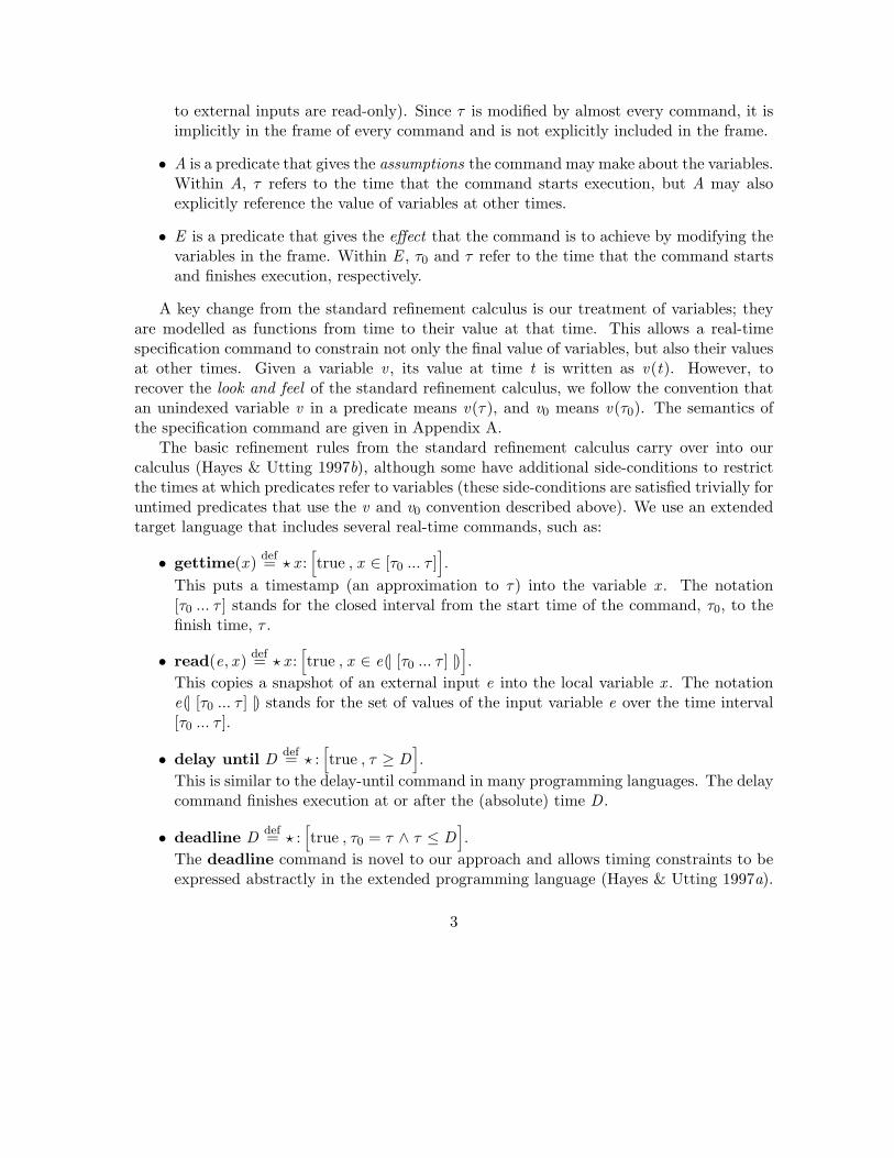
to external inputs are read-only). Since τ is modified by almost every command, it isimplicitly in the frame of every command and is not explicitly included in the frame.
• A is a predicate that gives the assumptions the command may make about the variables.Within A, τ refers to the time that the command starts execution, but A may alsoexplicitly reference the value of variables at other times.
• E is a predicate that gives the effect that the command is to achieve by modifying thevariables in the frame. Within E , τ0 and τ refer to the time that the command startsand finishes execution, respectively.
A key change from the standard refinement calculus is our treatment of variables; theyare modelled as functions from time to their value at that time. This allows a real-timespecification command to constrain not only the final value of variables, but also their valuesat other times. Given a variable v , its value at time t is written as v(t). However, torecover the look and feel of the standard refinement calculus, we follow the convention thatan unindexed variable v in a predicate means v(τ), and v0 means v(τ0). The semantics ofthe specification command are given in Appendix A.
The basic refinement rules from the standard refinement calculus carry over into ourcalculus (Hayes & Utting 1997b), although some have additional side-conditions to restrictthe times at which predicates refer to variables (these side-conditions are satisfied trivially foruntimed predicates that use the v and v0 convention described above). We use an extendedtarget language that includes several real-time commands, such as:
• gettime(x ) def= ? x :[true , x ∈ [τ0 ... τ ]
].
This puts a timestamp (an approximation to τ) into the variable x . The notation[τ0 ... τ ] stands for the closed interval from the start time of the command, τ0, to thefinish time, τ .
• read(e, x ) def= ? x :[true , x ∈ e(| [τ0 ... τ ] |)
].
This copies a snapshot of an external input e into the local variable x . The notatione(| [τ0 ... τ ] |) stands for the set of values of the input variable e over the time interval[τ0 ... τ ].
• delay until D def= ? :[true , τ ≥ D
].
This is similar to the delay-until command in many programming languages. The delaycommand finishes execution at or after the (absolute) time D .
• deadline D def= ? :[true , τ0 = τ ∧ τ ≤ D
].
The deadline command is novel to our approach and allows timing constraints to beexpressed abstractly in the extended programming language (Hayes & Utting 1997a).
3

The deadline command takes no time and must terminate at or before time D . Hence,it requires the preceding portion of the program to be complete by time D .
• idle def= ? :[true , τ0 ≤ τ
].
The idle command may take time but does not change any variables. Note thatexternal inputs may change during the time it takes to execute.
The presence of deadline commands means that a separate program analysis is required toguarantee that the deadlines will be met by the machine code generated for the program by acompiler. If the program analysis cannot guarantee that a deadline will be met, the programis rejected. Note that it is important to analyse timing after compilation, because no analysisof the higher-level program can take into account low-level aspects such as register allocationand code optimisation within a compiler, or instruction pipelining and cache memories withinprocessors, which together can significantly affect the timing characteristics of a program.
3 On measuring the size of a kiwifruit
Imagine that a single kiwifruit is moving along on a conveyor belt and goes through alight beam sensor that is connected into an embedded microcomputer. A program on themicrocomputer polls the boolean sensor status and uses a real-time clock to determine theapproximate start and end times of when the light beam is broken. When the kiwifruitbreaks the light beam the sensor rises (to true) and after the kiwifruit passes the light beamis re-established and the sensor falls (to false). From those times, and the known speed ofthe conveyor belt, the size of the kiwifruit can be computed.
The following declarations define the environment in which our program will be used. Aswell as documenting the type of variables representing physical quantities, we also documenttheir units (Hayes & Mahony 1995). Variables of type time are in units of nanoseconds.
const speed def= 10 m/s -- The speed of the conveyor beltconst react def= 100 µ s -- Desired reaction time after the kiwifruit passes
The sensor is an external input to the program. It is derived from the light beam detectinghardware. Its value over time is not under the control of the program, but the program doesmake assumptions about the behaviour of the input sensor.
input sensor : Bvar size : N nm -- Returned size of the kiwifruit in nanometres
The logical constants rises and falls are introduced solely for specification purposes. Theydenote, respectively, the exact time at which the sensor rises and falls. Logical constants
4

may not be used in the final program, except in assertions and deadlines.
con rises, falls : timeconstminsep def= 1 ms -- Minimum separation between rises and falls
-- Corresponds to length of 10 mm
The program may assume that the rise time precedes the fall time by a period of minsep.
?{rises + minsep ≤ falls
}(1)
Because (1) does not refer to any variables modified by the program, it may be assumedto hold throughout the program. To avoid cluttering the specification and the refinementbelow, we state (1) once here and assume it where needed. Logically it could be conjoined tothe assumption of the specification (2) below and passed through the refinement as necessary.The sensor detects (is true) when the light beam is interrupted by the passing kiwifruit.
SENSOR(τ) def= (∀ t : [τ ... falls + react ] • sensor(t) = true ⇔ t ∈ [rises ... falls])
The top level specification is:
? size:
[τ ≤ risesSENSOR(τ)
,τ ≤ falls + reactsize ∈ speed ∗ (falls − rises)± 1 mm
](2)
4 Refinement of the kiwifruit sizer
Appendix A provides a summary of refinement laws used within this paper.As a first refinement step, it is useful to separate out the initial time assumption, τ ≤
rises, and the final deadline requirement, τ ≤ falls + react , so that we may concentrate onimplementing the remaining functionality.
(2)v Law 6 (separate assumption); Law 10 (separate deadline)
?{τ ≤ rises
};
? size:[SENSOR(τ) , size ∈ speed ∗ (falls − rises)± 1 mm
]; (3)
deadline falls + react
The assertion and deadline become part of the final program, and we are left to refine thespecification command (3).
The next main refinement step is obvious – we want to split the program into three parts:the first two will determine the rise and fall times as accurately as possible and the third
5

part computes the size output. We introduce a constant err as an error bound on the timeto detect the change in the sensor. We leave the actual value of err to be determined later,but at this stage we require that it is less than both minsep and react , so that the sensor isstable for at least a period of err after it changes.
const err ∈ {t : time | t ≤ minsep ∧ t ≤ react} (4)
Local variables riset and fallt are used to communicate the approximations to the riseand fall times between the parts. When introducing a local variable one cannot assume thatthe allocation and deallocation of the local variable take no time. Hence, an assumption thatheld immediately before the allocation of a local variable, may not hold immediately afterthe allocation. However, during the allocation of a new variable the other program variables(not including the external inputs) are stable and time can only increase. A predicate thatremains true under these circumstances is referred to as being idle-stable. It is invariant overthe execution of an idle command. The predicate SENSOR(τ) is idle-stable. It states aproperty that holds at every instant of time from τ up to falls + react . Hence, SENSOR(x )also holds for all values of x later than τ .
The time taken for the allocation and deallocation of variables also affects the effect ofthe specification command. In this case the effect only refers to constants and the programvariable size. Because size is stable during the deallocation of the variables, the effect willstill be true after the deallocation.
Note that we follow Morgan’s (1994) convention of using a � symbol to mark the speci-fication statement that is refined next – the context of that statement becomes the contextof the next refinement.
(3)v Law 11 (introduce variable)
|[var riset , fallt : time;
? size, riset , fallt :[SENSOR(τ) , size ∈ speed ∗ (falls − rises)± 1 mm
]�
]|v Law 9 (simple sequential composition) × 2; Law 5 (remove from frame) × 3
? riset :
[SENSOR(τ) ,
SENSOR(τ)riset ∈ [rises ... rises + err ]
]; (5)
? fallt :
[SENSOR(τ)riset ∈ [rises ... rises + err ]
,riset ∈ [rises ... rises + err ]fallt ∈ [falls ... falls + err ]
]; (6)
? size:
[riset ∈ [rises ... rises + err ]fallt ∈ [falls ... falls + err ]
, size ∈ speed ∗ (falls − rises)± 1 mm
](7)
6

The refinement of (5) is more interesting. The goal is to determine the time at whichthe light beam sensor rises. Our first step is to massage the specification to reflect thismore specific goal. Firstly, the effect SENSOR(τ) is immediate from the assumption becauseSENSOR(τ) is an idle-stable predicate that does not refer to the variable in the frame, riset .Secondly, we weaken the assumption so that we only consider the rising phase of the signal.
(5)v Law 4 (strengthen effect); Law 3 (weaken assumption)
? riset :
[∀ t : [τ ... rises + err ] •
sensor(t) = true ⇔ rises ≤ t, riset ∈ [rises ... rises + err ]
](8)
We make use of the following definition which is written to allow detection of either a risingedge (the new sensor value we are required to detect, srqd , is true), or a falling edge change(srqd = false).
CHNG(chngs, srqd) def= ∀ t : [τ ... chngs + err ] • sensor(t) = srqd ⇔ chngs ≤ t
To refine the detection of the rise of the sensor, we make use of a procedure, detect chng .The first step is a refinement equivalence (vw).
(8)
vw ? riset :[CHNG(rises, true) , riset ∈ [rises ... rises + err ]
]v parametrized procedure
detect chng(rises, true, riset)
The procedure detect chng can be used to detect either a rising or falling edge of the sensorvalue depending on the parameter srqd , which is the required new value of the sensor.
proc detect chng(con chngs : time; value srqd : B; result chngt : time) def=
? chngt :[CHNG(chngs, srqd) , chngt ∈ [chngs ... chngs + err ]
](9)
Before giving a refinement of detect chng (see the next section) we complete the refinementof the program. Detecting the falling edge also makes use of the procedure detect chng .
(6)v Law 4 (strengthen effect); Law 3 (weaken assumption)
? fallt :[CHNG(falls, false) , fallt ∈ [falls ... falls + err ]
]v parametrized procedure
detect chng(falls, false, fallt)
7

Once both the rise time and the fall time have been determined, the size of the kiwifruit canbe calculated.
(7)v Law 7 (assignment)
size := speed ∗ (fallt − riset)
The units of the right side expression are (m / s) ∗ ns = nm, which matches the units of size.The proof obligation for the last step is
speed ∗ (fallt − riset) ∈ speed ∗ (falls − rises)± 1 mm≡ fallt − riset ∈ (falls − rises)± (1 mm /speed)W from the assumptions on riset and fallt
[falls − (rises + err) ... (falls + err)− rises] ⊆ (falls − rises)± (1 mm /speed)≡ (falls − rises)± err ⊆ (falls − rises)± (1 mm /speed)≡ err ≤ (1 mm /speed)≡ err ≤ 100 µ s
That gives the final constraint on err .
5 Refinement of detection of a sensor change
The following code is the implementation of detect chng (the refinement to this code followsshortly). Note that this code is similar to what a programmer would write for this task,except that deadline commands have been added to make the timing requirements of theprogram explicit.
proc detect chng(con chngs : time; value srqd : B; result chngt : time) v|[var sens : B ;
read(sensor , sens) ;deadline chngs + err ;?do sens 6= srqd →
read(sensor , sens) ;deadline chngs + err
od ;gettime(chngt) ;deadline chngs + err
]|
8

Aside: The above code corresponds to what is usually referred to as busy waiting. Inthe current context we are assuming a single sequential process, and hence busy waiting isacceptable. It would also be acceptable to include a (sampling) delay in the above code,provided the delay time is sufficiently short to allow the program to meet its deadlines. Wehave not done so here.
The final deadline ensures that the captured change time is within its allowable errorbounds. Given the last deadline, the first two deadlines seem redundant, but they areessential for the correct operation of the program. The final deadline command will not bereached by the program if the loop does not terminate, and if the deadline is not reached, itdoes not have to be met. Consider the case where we want to detect the rise of the sensor.Without the first deadline the initial code could take so long that the first read commandcompletely misses the period when the sensor is true. (This is unlikely in practice, butnot excluded by the meanings we have given to the programming constructs.) If the firstread completely misses the sensor when it is raised, then the loop will not be guaranteedto terminate, because our assumptions only guarantee one period when the sensor is raised.Hence the final deadline may never be reached. The deadline within the loop has a similarpurpose. It guarantees that the body of the loop will not take so long that the read of thesensor misses the raised period of the sensor. Again, if the raised period were missed theloop would not be guaranteed to terminate, and the final deadline would not be reached.As we shall see shortly, the refinement process needs to introduce the deadlines in order toguarantee that the specification will be met. In addition, the deadline within the loop is alsoused to guarantee its termination.
Before continuing, we invite the reader to informally analyse this code (e.g., unroll theloop once or twice) to determine the longest path through the code that can be executedfrom time chngs to the gettime command. Note how the analysis depends on consequencesof CHNG(chngs, srqd), such as the shape of the sensor waveform. Our real-time calculusenables us to make these implicit timing assumptions and invariants explicit, so that we canprovide an invariant for the loop and so that the timing analysis phase has a manageabletask. With these goals in mind, it turns out (after several attempts!) that a suitable loopinvariant is:
INV def= CHNG(chngs, srqd) ∧ (sens = srqd ⇒ chngs ≤ τ)
The first step is to introduce a local variable, sens, that is used to capture the sensor’s values.
(9)v Law 11 (introduce variable)
|[var sens : B;
? chngt , sens:[CHNG(chngs, srqd) , chngt ∈ [chngs ... chngs + err ]
](10)
]|
9

Next we set up a loop that searches for the change of the sensor and then we capture thetime. The introduction of the loop makes use of the following law, that does not havea conventional variant to show termination. Our semantics of the loop guarantees thateach iteration takes a minimum amount of time, due for example to loop overheads andguard evaluation. Termination is guaranteed by the fact that time increases by at least thatminimum amount on each iteration, and every iteration of the body of the loop is bounded bythe same constant time limit. The time limit, L, is required to be frame-stable with respectto the frame, ~x , of the loop. That guarantees that L will remain invariant (stable) duringthe execution of the loop. If L does not refer to variables in the frame, or τ , or externalinputs, then it is frame-stable.
Law 1 (iteration with deadline) Given an idle-stable invariant property, INV , a dead-line expression L, which is frame-stable with respect to the frame ~x , and an idle-stable expres-sion G, where none of G, L and INV contain references to τ0 or zero-subscripted variables,
?~x :[INV ∧ τ ≤ L, ¬ G ∧ INV
]v ?doG → ?~x :
[G ∧ INV , INV ∧ τ ≤ L
]od
The semantics of loops and the proof of this law are contained in Appendix B. Beforeintroducing the loop, we separate the initialisation, loop, and final capture of the changetime.
(10)v Law 9 (simple sequential composition) × 2; Law 5 (remove from frame) × 3
? sens:[CHNG(chngs, srqd) , INV ∧ τ ≤ chngs + err
]; (11)
? sens:[INV ∧ τ ≤ chngs + err , INV ∧ sens = srqd
]; (12)
? chngt :[INV ∧ sens = srqd , chngt ∈ [chngs ... chngs + err ]
](13)
The initialisation establishes the loop invariant. In the second refinement step below, becauseof the assumption, if the value sensed is equal to srqd then the completion time of thecommand must be after chngs. If the sensed value is not equal to srqd the completion timemay be either before or after chngs, but that does not matter.
(11)v Law 4 (strengthen effect)
? sens:
[∀ t : [τ ... chngs + err ] •
sensor(t) = srqd ⇔ chngs ≤ t,sens = srqd ⇒ chngs ≤ ττ ≤ chngs + err
]v Law 4 (strengthen effect)
? sens:
[∀ t : [τ ... chngs + err ] •
sensor(t) = srqd ⇔ chngs ≤ t,sens ∈ sensor(| [τ0 ... τ ] |)τ ≤ chngs + err
]
10

v Law 3 (weaken assumption); Law 10 (separate deadline); Definition of readread(sensor , sens) ; deadline chngs + err
Now we can introduce the loop.
(12)v Law 1 (iteration with deadline)
?do sens 6= sqrd→
? sens:[sens 6= srqd ∧ INV , INV ∧ τ ≤ chngs + err
]�
od
v Law 3 (weaken assumption)
? sens:[CHNG(chngs, srqd) , INV ∧ τ ≤ chngs + err
]v as for the refinement of (11)
read(sensor , sens) ; deadline chngs + err
On termination the change of the sensor has been detected. It only remains to capturethe current time, before the allowed error bound.
(13)v Law 3 (weaken assumption)
? chngt :[chngs ≤ τ , chngt ∈ [chngs ... chngs + err ]
]v Law 4 (strengthen effect)
? chngt :[chngs ≤ τ , chngt ∈ [τ0 ... τ ] ∧ τ ≤ chngs + err
]v Law 10 (separate deadline); Law 3 (weaken assumption); Definition of gettime
gettime(chngt) ; deadline chngs + err
The final program, with the procedure detect chng inlined is shown in Figure 1.
6 Timing analysis
The final phase is to determine the time constraints on paths through the code in orderto guarantee that all deadlines will be met. For each deadline command we consider thepaths through the program that terminate at the deadline. For each such path we needto determine a time constraint on the execution time of the path that guarantees that thedeadline will be met. Grundon, Hayes & Fidge (1998) have formalised the details of timingpath analysis, but here we present a brief overview of the process for the program in Figure 1.
11

A :: ?{τ ≤ rises
};
|[var riset , fallt : time;
|[var sens : B;read(sensor , sens);
B :: deadline rises + err ;?do invariantCHNG(rises, true) ∧ (sens = true ⇒ rises ≤ τ)sens 6= true →
read(sensor , sens);C :: deadline rises + errod ;gettime riset ;
D :: deadline rises + err
]|;|[var sens : B;
read(sensor , sens);E :: deadline falls + err ;
?do invariantCHNG(falls, false) ∧ (sens = false ⇒ falls ≤ τ)sens 6= false →
read(sensor , sens);F :: deadline falls + errod ;gettime fallt ;
G :: deadline falls + err
]|;size := speed ∗ (fallt − riset)
]|;H :: deadline falls + react
Figure 1: Final program with the procedure inlined.
12

The first path we consider is A–B, which has a start time before1 rises and must completebefore rises + err . That gives a time constraint for the path of err . Both path A–C, whichenters the loop on the first iteration, and path A–D, which does not enter the loop at all,have the same constraint of err .
The path starting at A that enters the loop for the first iteration is not the only path thatends at C. The other possibilities come from the repetition of the loop. These paths requiresome intricate reasoning to determine suitable time constraints. Our goal is to determinetiming constraints on paths through the code that guarantee that the deadline at point C isreached before its deadline of rises + err . Because the deadline is within the loop body, weknow on entry to the loop that sens is false, which implies that the previous read must havecommenced before time rises. Hence our constraint is that the path from the previous read,around the loop through the current read, and finishing at the deadline at C, must take timeless than rises + err − rises = err .
There are paths from D to E, F and G. All start no later than rises + err and mustcomplete before falls + err . That gives them a time constraint of falls − rises. However, weare guaranteed by (1) that falls − rises ≥ minsep, and hence we can use minsep as our timeconstraint.
The remainder of the paths for calculating the fall time of the sensor are similar to thosefor calculating the rise. We do not discuss them in detail here.
The final path that we consider is G–H. It has a start time before falls + err and mustcomplete before falls + react . This gives a time constraint of react − err . The specificationgives react as 100 µ s, and our refinement requires that err ≤ 100 µ s. The constant errappears in the constraints of many paths. It can be chosen up to the limit of 100 µ s so thatthe paths can meet their timing constraints.
Provided we can show that the machine code generated for each of the above pathssatisfies the corresponding time constraint, then we can guarantee all deadlines will be met.There has been considerable research in the real-time community on timing analysis of suchmachine code sequences (Lim et al. 1995).
7 Conclusions
The main advantage of the sequential real-time refinement calculus presented here is that, todevelopers, it appears to be a straightforward extension of the standard refinement calculus.Although it has a different underlying semantics, most of the standard refinement lawscarry over, and the real-time extended programming language is a superset of the standardtarget language. In practice, a development in the real-time calculus is similar to standardrefinement calculus development, but with the addition of steps to separate out timingconstraints and refine them into real-time language constructs.
1To simplify presentation ‘before’ is taken to mean ‘no later than’ throughout this section.
13

However, even with this strong connection to the standard calculus, our experience so farsuggests that programs that rely heavily on timing behaviour for their correctness are quitechallenging to develop in our calculus. Finding loop invariants and sequential compositionintermediate predicates seems more difficult than in the standard calculus. We suspectthat this is partly because we have had more experience with the standard calculus, andpartly because real-time programming is intrinsically difficult. Certainly the timing analysisphase is an additional requirement with its own intricacies. Anyway, it is exciting to have acalculus that allows the subtle aspects of real-time programs to be formally proved, just asthe standard calculus “dots the i’s and crosses the t’s” of ordinary sequential programming.
References
Back, R.-J. (1980), Correctness preserving program refinements: Proof theory and applica-tions, Tract 131, Mathematisch Centrum, Amsterdam.
Grundon, S., Hayes, I. J. & Fidge, C. J. (1998), Timing constraint analysis, in C. McDonald,ed., ‘Computer Science ’98: Proc. 21st Australasian Computer Sci. Conf. (ACSC’98),Perth, 4–6 Feb.’, Springer, pp. 575–586.
Hayes, I. J. & Mahony, B. P. (1995), ‘Using units of measurement in formal specifications’,Formal Aspects of Computing 7(3), 329–347.
Hayes, I. J. & Utting, M. (1997a), Coercing real-time refinement: A transmitter, inD. J. Duke & A. S. Evans, eds, ‘BCS-FACS Northern Formal Methods Workshop(NFMW’96)’, Springer.
Hayes, I. J. & Utting, M. (1997b), A sequential real-time refinement calculus, Technical Re-port UQ-SVRC-97-33, Software Verification Research Centre, The University of Queens-land, URL http://svrc.uq.edu.au.
Lim, S.-S., Bae, Y. H., Jang, G. T., Rhee, B.-D., Min, S. L., Park, C. Y., Shin, H., Park,K., Moon, S.-M. & Kim, C. S. (1995), ‘An accurate worst case timing analysis for RISCprocessors’, IEEE Trans. on Software Eng. 21(7), 593–604.
Mahony, B. P. (1992), The Specification and Refinement of Timed Processes, PhD thesis,Department of Computer Science, University of Queensland.
Morgan, C. C. (1994), Programming from Specifications, second edn, Prentice Hall.
Utting, M. & Fidge, C. J. (1996), A real-time refinement calculus that changes only time, inHe Jifeng, ed., ‘Proc. 7th BCS/FACS Refinement Workshop’, Electronic Workshops inComputing, Springer.
14

Utting, M. & Fidge, C. J. (1997), Refinement of infeasible real-time programs, in ‘Proc.Formal Methods Pacific ’97’, Springer, Wellington, New Zealand, pp. 243–262.
A Laws for language constructs
The following laws are extracted from an earlier paper (Hayes & Utting 1997b) that givesthe semantics of the real-time language constructs, as well as a more comprehensive set oflaws.
Unindexed variables in predicates and expressions In a predicate, unindexed vari-ables of the form v stand for v(τ), and variables of the form v0 stand for v(τ0). We introducethe notation R @ (τ0, τ) to stand for the predicate R with every unindexed occurrence of avariable, v , replaced by v(τ) and every occurrence of v0 replaced by v(τ0). Note that R maycontain explicit indexed references to variables at times other than τ ; these are not affectedby the ‘@’ operator. The operator ‘@’ has a lower precedence than all the normal logicaloperators, but a higher precedence than ‘≡’ and ‘V’. For predicates, such as assumptions,that do not contain any zero-subscripted variables, we use the notation P @τ . If there are nooccurrences of τ0 or zero-subscripted variables in P then P @ (τ0, τ) ≡ P @ τ . The operator‘@’ distributes over logical operators.
Specifications The assumptions of a specification command determine the range of possi-ble values of variables over time, as well as the start time of the command. The effect furtherconstrains the values of variables over time, as well as constraining the finish time of thecommand. Program variables (local variables and outputs) not in the frame of a specificationare stable over its execution. Given a variable, v , and a set of times, S ,
stable(v ,S ) def= (∀ t , u : S • v(t) = v(u))
The meaning of a specification command is given with respect to a given environment,where an environment just records the variables (inputs, outputs and local variables) thatare in scope. We use ρ to stand for an environment, and ρ̂ to stand for the program variables(outputs and local variables) within ρ. The meaning function, Mρ, gives the meaning of areal-time construct in environment ρ in terms of a predicate transformer determined by astandard refinement calculus construct.
Definition 2 (specification) A specification command, ?~x :[P , R
], is well formed in an
environment, ρ, provided (i) the frame, ~x , is a vector of program variables (outputs and localvariables), (ii) P is a predicate involving the variables in the environment plus τ , and (iii) Ris a predicate involving variables in the environment plus τ0, τ and zero-subscripted versions
15

of variables in the environment. The meaning of a well-formed specification command isgiven by the following
Mρ
(?~x :
[P , R
])def= τ :
[P @ τ , R @ (τ0, τ) ∧ τ0 ≤ τ ∧ stable(ρ̂ \ ~x , [τ0 ... τ ])
]where ρ̂ \ ~x stands for the program variables, ρ̂, with any elements in the frame ~x removed.
Note that τ , unlike other variables, is not itself a function of time. The frame, ~x , of the real-time command does not appear in the frame of the equivalent standard command. Instead,those program variables that are not in the frame are constrained to be stable for its duration,and the program variables in the frame are only constrained by the effect of the specification,R. In the assumption and effect of a specification command it is permissible to include bothexplicitly indexed references and unindexed references to the same variable. For more detailson the encoding of real-time specifications the reader is referred to Utting & Fidge (1997).
The refinement rules for weakening an assumption and strengthening an effect carry overto the real-time refinement calculus.
Law 3 (weaken assumption) Provided P @ τ V P ′ @ τ ,
?~x :[P , R
]v ?~x :
[P ′, R
].
When applying this law we can use the fact that from P V P ′ one can deduce that P @ τ VP ′ @ τ . That gives a special case of the law for dealing with properties that are not timedependent.
Law 4 (strengthen effect) Given an environment, ρ, provided
(P @ τ0) ∧ (R′ @ (τ0, τ)) ∧ τ0 ≤ τ ∧ stable(ρ̂ \ ~x , [τ0 ... τ ]) V R @ (τ0, τ)
then
?~x :[P , R
]v ?~x :
[P , R′
]where ρ̂ \~x stands for the program variables (local variables and outputs) of the environmentρ, minus the variables in the frame, ~x .
In the case where the properties are not time dependent, a special case of the proviso is,P0 ∧ R′ V R, where P0 stands for the predicate P with all occurrences of τ replaced byτ0, and all unindexed occurrences of every variable, v , that is in the frame or is an externalinput, replaced by v0.
Law 5 (remove from frame) Given disjoint vectors of program variables, ~x and ~v,
?~x , ~v :[P , R
]v ?~v :
[P , R
]16
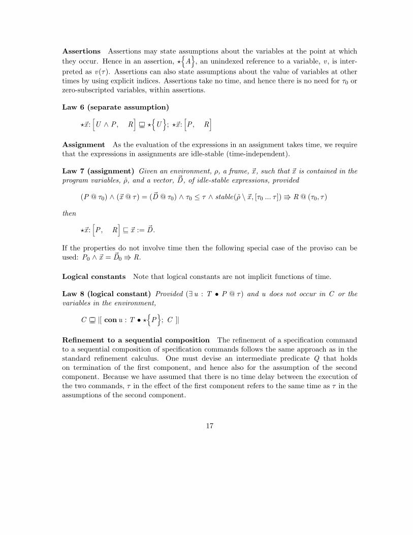
Assertions Assertions may state assumptions about the variables at the point at whichthey occur. Hence in an assertion, ?
{A
}, an unindexed reference to a variable, v , is inter-
preted as v(τ). Assertions can also state assumptions about the value of variables at othertimes by using explicit indices. Assertions take no time, and hence there is no need for τ0 orzero-subscripted variables, within assertions.
Law 6 (separate assumption)
?~x :[U ∧ P , R
]vw ?
{U
}; ?~x :
[P , R
]Assignment As the evaluation of the expressions in an assignment takes time, we requirethat the expressions in assignments are idle-stable (time-independent).
Law 7 (assignment) Given an environment, ρ, a frame, ~x , such that ~x is contained in theprogram variables, ρ̂, and a vector, ~D, of idle-stable expressions, provided
(P @ τ0) ∧ (~x @ τ) = (~D @ τ0) ∧ τ0 ≤ τ ∧ stable(ρ̂ \ ~x , [τ0 ... τ ]) V R @ (τ0, τ)
then
?~x :[P , R
]v ~x := ~D .
If the properties do not involve time then the following special case of the proviso can beused: P0 ∧ ~x = ~D0 V R.
Logical constants Note that logical constants are not implicit functions of time.
Law 8 (logical constant) Provided (∃ u : T • P @ τ) and u does not occur in C or thevariables in the environment,
C vw |[ con u : T • ?{P
}; C ]|
Refinement to a sequential composition The refinement of a specification commandto a sequential composition of specification commands follows the same approach as in thestandard refinement calculus. One must devise an intermediate predicate Q that holdson termination of the first component, and hence also for the assumption of the secondcomponent. Because we have assumed that there is no time delay between the execution ofthe two commands, τ in the effect of the first component refers to the same time as τ in theassumptions of the second component.
17

Law 9 (simple sequential composition) Provided Q and R do not involve τ0 or zero-subscripted variables,
?~x :[P , R
]v ?~x :
[P , Q
]; ?~x :
[Q , R
]A timing deadline in the effect of a specification command may be separated out into a
deadline command.
Law 10 (separate deadline) Provided D is a time-valued expression, which may includereferences to logical constants but no references to τ0 or zero-subscripted variables,
?~x :[P , R ∧ τ ≤ D
]v ?~x :
[P , R
]; deadlineD
Local variables The definition of a local variable block in the real-time language involvesexpanding the environment for the command within the block. The allocation and deal-location of local variables may take time. Hence we need stability requirements on theassumption and effect in the variable introduction law.
Law 11 (introduce variable) Given an environment, ρ, such that v does not occur in thevariables of ρ (and hence does not occur free within P or R or in ~x), provided T is nonempty,P is idle-stable and R is both pre- and post-idle-stable, then
?~x :[P , R
]vw |[ var v : T • ?v , ~x :
[P , R
]]|
A predicate R is pre-idle-stable (post-idle-stable) if when R is used as an effect of a specifica-tion command, the specification command can be prefixed (postfixed) by an idle commandand the result is a refinement of the original specification command (Hayes & Utting 1997b).
B Iteration
We distinguish between the real-time iteration command (?do) and the standard iterationcommand (do) within this section and use the latter in the definition of the former as a wayof reusing its predicate transformer.
The guard of an iteration is required to be idle-stable so that it is stable during itsevaluation. To account for the delay to evaluate the guard an idle command with a minimumexecution time (d1) is used,
idle≥d1def= ? :
[true , τ − τ0 ≥ d1
]and to account for exiting the loop, an idle command with a maximum execution time (d2)is used,
idle≤d2def= ? :
[true , τ − τ0 ≤ d2
]18

Of course, both d1 and d2 are dependent on the implementation, but our definition does notrely on the particular values of these, just that such constants exist. To allow for the casewhen the guard is initially false, an idle is added after the loop to allow the loop to takesome time in this case.
Definition 12 (iteration) Given an environment, ρ, and an idle-stable expression, G,which does not contain references to τ0 or zero-subscripted variables,
Mρ (?doG → C od) def=ud1, d2 : Time | d1 > 0 ∧ d2 > 0 •
doG @ τ →Mρ (idle≥d1; C ; idle≤d2) od ◦Mρ (idle)
where ‘u’ is generalised nondeterministic choice and ‘◦’ is standard sequential composition.
The following loop introduction rule does not make use of a conventional variant toshow termination. Instead it makes use of a fixed deadline that does not change during theexecution of the loop. When combined with the inevitable progress of time due to executionof the loop, this has the same effect as a variant.
Law 13 (iteration timing with deadline) Given an idle-stable invariant property, INV ,a deadline expression, L, which is frame-stable with respect to the frame ~x , idle-stable expres-sions G and D, and an environment, ρ, where none of G, D, L and INV contain referencesto τ0 or zero-subscripted variables,
?~x :[INV ∧ D = τ ≤ L, ¬ G ∧ INV ′
]v ?doG → ?~x :
[G ∧ INV ′, INV ′ ∧ τ ≤ L
]od
where INV ′ def= INV ∧ D ≤ τ ∧ stable(ρ̂ \ ~x , [D ... τ ]).
Proof Our first step is to introduce the idle command at the end of Definition 12 (itera-tion). The introduction relies on ¬ G ∧ INV ′ being post-idle-stable.
?~x :[INV ∧ D = τ ≤ L, ¬ G ∧ INV ′
]vw Law 9 (simple sequential composition); Definition of idle
?~x :[INV ∧ D = τ ≤ L, ¬ G ∧ INV ′
]; idle
We now proceed to refine the first component using the standard refinement calculus laws.To emphasise this we use the s-subscripted ‘vs ’ to stand for refinement in the standardcalculus.
Mρ
(?~x :
[INV ∧ D = τ ≤ L, ¬ G ∧ INV ′
])19

vws Definition 2 (specification)
τ :[INV ∧ D = τ ≤ L @ τ , ¬ G ∧ INV ′ @ (τ0, τ) ∧ τ0 ≤ τ ∧ stable(ρ̂ \ ~x , [τ0 ... τ ])
]vs definition of INV ′; strengthen postcondition; weaken precondition; choice
[] d1, d2 : Time | d1 > 0 ∧ d2 > 0 •
τ :[INV ′ ∧ τ ≤ L + d2 @ τ , ¬ G ∧ INV ′ ∧ τ ≤ L + d2 @ τ
]�
vs Standard iteration with variant⌊
L+d2−τd1
⌋doG @ τ →
τ :
[G ∧ INV ′ ∧ τ ≤ L + d2 @ τ ,
INV ′ ∧ τ ≤ L + d2 @ τ ∧⌊L+d2−τ
d1
⌋<
⌊L+d2−τ0
d1
⌋ ]od
vs definition of INV ′; weaken precondition; strengthen with τ0 ≤ τ
doG @ τ →
τ :
[G ∧ INV ′ @ τ ,
INV ′ ∧ τ0 + d1 ≤ τ ≤ L + d2 @ (τ0, τ)τ0 ≤ τ ∧ stable(ρ̂ \ ~x , [τ0 ... τ ])
]od
vws Definition 2 (specification)
doG @ τ →Mρ
(?~x :
[G ∧ INV ′, INV ′ ∧ τ0 + d1 ≤ τ ≤ L + d2
])od
We now concentrate on the body of the loop. The following step relies on the fact thatG ∧ INV ′ is idle-stable, and that INV ′ is both pre- and post-idle-stable.
?~x :[G ∧ INV ′, INV ′ ∧ τ0 + d1 ≤ τ ≤ L + d2
]v Law 9 (simple sequential composition) × 2; Definitions of idles
idle≥d1; ?~x :[G ∧ INV ′, INV ′ ∧ τ ≤ L
]; idle≤d2
Combining the above together we get,
[] d1, d2 : Time | d1 > 0 ∧ d2 > 0 •doG @ τ →Mρ
(idle≥d1; ?~x :
[G ∧ INV ′, INV ′ ∧ τ ≤ L
]; idle≤d2
)od ◦Mρ (idle)
vws Definition 12 (iteration)Mρ
(?doG → ?~x :
[G ∧ INV ′, INV ′ ∧ τ ≤ L
]od
)2
A simpler rule for iteration does not involve all timing aspects.
20

Law 1 (iteration with deadline) Given an idle-stable invariant property, INV , a dead-line expression L, which is frame-stable with respect to the frame ~x , and an idle-stable expres-sion G, where none of G, L and INV contain references to τ0 or zero-subscripted variables,
?~x :[INV ∧ τ ≤ L, ¬ G ∧ INV
]v ?doG → ?~x :
[G ∧ INV , INV ∧ τ ≤ L
]od
Proof We let INV ′ def= INV ∧ D ≤ τ ∧ stable(ρ̂ \ ~x , [D ... τ ]), where D is fresh, and makeuse of Law 13 (iteration timing with deadline).
?~x :[INV ∧ τ ≤ L, ¬ G ∧ INV
]v Law 8 (logical constant); Law 6 (separate assumption); Law 4 (strengthen effect)|[ conD : Time • ?~x :
[INV ∧ D = τ ≤ L, ¬ G ∧ INV ′
]]|
vw Law 13 (iteration timing with deadline)|[ conD : Time • ?doG → ?~x :
[G ∧ INV ′, INV ′ ∧ τ ≤ L
]od ]|
vw Equivalent effect by Law 4 (strengthen effect); Law 3 (weaken assumption)|[ conD : Time • ?doG → ?~x :
[G ∧ INV , INV ∧ τ ≤ L
]od ]|
vw Law 8 (logical constant)?doG → ?~x :
[G ∧ INV , INV ∧ τ ≤ L
]od
2
21