Embed Size (px)
Citation preview

QA: QA
SOFTWARE USERS MANUAL (UM)for the
FEHM Application Version 2.21
STN: 10086-2.21-00
REV. NO. 00
DOCUMENT ID: 10086-UM-2.21-00
October 2003Effective date
Prepared by:
Zora V. Dash
Los Alamos National Laboratory, EES-6
Date
Verified by:
Myles FitzgeraldLos Alamos National Laboratory, EES-9
Date
Fred PollockBechtel SAIC, LLCSoftware Independent Verification & Validation
Date
Los Alamos National Laboratory

1006b-UM-2.21-00 FE]IM V2.21 Users Manual QA: QAPage: 2 of 189
Copyright, 2003, The Regents of the University of California.
This program was prepared by the Regents of the University of California at Los Aletpos NationalLaboratory (the University) under contract No. W-7405-ENG-36 with the U. S. bepa4,1" ent of Energy
(DOE). All rights in the program are reserved by the DOE and the University, rrIsoni grated tothe
public to copy and use this software without charge, provided that this Notice •nd t statement ofauthorship are reproduced on all copies. Neither the U.S. Government nor the& 'rns'Aity make anywarranty, express or implied, or assumes any liability or responsibility for the: tse Ch ii~is sokware.

10086-UM-2.21-00
CHANGE HISTORY
FEHM V2.21 Users Manual QA: QAPage: 3 of 189
RevisionNumber
2.21-00
EffectiveDate
9/16/03
Description of and Reason for Revision
Initial revision, based on AP-SI. 1Q.

10086-UM-2.21-00 FEHM V2.21 Users Manual QA: QAPage: 4 of 189
TABLE OF CONTENTS
LIST OF FIGURES ...............................
LIST OF TABLES .................................
1.0 PURPOSE ..................................
2.0 DEFINITIONS AND ACRONYMS .................2.1 Definitions ..........................2.2 Acronyms ...............................
3.0 REFERENCES ..............................
4.0 PROGRAM CONSIDERATIONS ................4.1 Program Options ....... ..............4.2 Initialization ..................... .....4.3 Restart Procedures....................4.4 Error Processing ..........................
.. 8
.. 8.. 8
.8
.10.. 10.. 11
..11
5.0 DATA FILES .............................5.1 Control file (iocntl) ......................5.2 Input file (inpt).........................5.3 Geometry data file (incoor) ...............5.4 Zone data file (inzone) ..................5.5 Optional input files .......................5.6 Read file (iread) ........................5.7 Multiple simulations input file ..............5.8 Type curve data input file. ...............5.9 Output file (iout) ........................5.10 W rite file (isave) .......................5.11 History plot file (ishis) ..................5.12 Solute plot file (istrc) ...................5.13 Contour plot file (iscon) .................5.14 Contour plot file for dual or dpdp (isconl)...5.15 Stiffness matrix data file (isstor) ..........5.16 Input check file (ischk) ..................5.17 Submodel output file (isubm) .............5.18 Output error file (ierr) ....................5.1.9 Multiple simulations script files ...........5.20 PEST output files (ispest, ispstl) .........
...............
.....I .........
...............
...............
...............
...............
...............
...............
...............
...............
...............
...............
...............
......... 17
......... 17
......... 17
......... 17
......... 18
......... 18
......... 18
......... 19....... .19
......... 19
......... 20
........ ..20
......... 20
......... 21
......... 21
......... 21
......... 22
......... 22
......... 22
......... 23
......... 23
......... 23
......... 24
......... 24
5.21 Streamline particle tracKing output Tiles (isptrl, ispirz, Isptri)...5.22 SURFER and TECPLOT output files ......................5.23 Advanced Visual Systems (AVS) output files ...............

10086-UM-2.21-00 FEHM V2.21 Users Manual QA: QAPage: 5 of 189
6.0 INPUT DATA ..................................................... 276.1 General Considerations ......................................... 276.2 Individual Input Records or Parameters ............................. 33
7.0 O UTPUT ....................................................... 1497.1 Output file (filen.out) ........................................... 1497.2 Write file (filen.fin) ................................... 1497.3 History plot file (filen.his) ........................................ 1517.4 Solute plot file (filen.trc). ................................. 1527.5 Contour plot file (filen.con) ...................................... 1527.6 Contour plot file for dual or dpdp (filen.dp) .......................... 1537.7 Stiffness matrix data (filen.stor) .................................. 1537.8 Input check file (filen.chk) ................................ 1547.9 Submodel output file (filen.subbc) ................................. 1547.10 Error output file (fehmn.err) ..................................... 1547.11 Multiple simulations script files (fehmn.pre, fehmn.post) ............... 1547.12 PEST output files (filen.pest, filen.pestl) .......................... 1547.13 Streamline particle tracking output files (filen.sptrl, filen.sptr2, filen.sptr3) 1557.14 SURFER and TECPLOT output files (surzonenumber.txt,
veczonenumber.txt, trczonenumber.txt or teczonenumber.plt,veczonenumber.plt, trczonenumber.pt) . ................... 156
7.15 AVS log output file (filen. 10001_avs log) .......................... 1577.16 AVS header output files (filen.numberjtype._head) ................... 1577.17 AVS geometry output file (fi/en. 10001_geo) ........................ 1577.18 AVS data output files (filen.numberjtype.node) ..................... 158
8.0 SYSTEM INTERFACE ............................................ 1608.1 System-Dependent Features .................................... 1608.2 Compiler Requirements. ................................... 1608.3 Hardware Requirements ........................................ 1608.4 Control Sequences or Command Files ............................. 1608.5 Software Environment .......................................... 1608.6 Installation Instructions . ................................... 160
9.0 EXAMPLES AND SAMPLE PROBLEMS ............................. 1629.1 Constructing an Input File.. ....................... 1629.2 Code Execution.. ....................... ................ 1659.3 Heat Conduction in a Square.................... 1709.4 DOE Code Comparison Project, Problem 5, Case A ................ 1779.5 Reactive Transport Example ................................ 182
10.0 USER SUPPORT ........ . ......... ............................ 189

10086-UM-2.21-00 FEHM V2.21 Users Manual QA: QAPage: 6 of 189
LIST OF FIGURES
Figure 1. AVS UCD formatted FEHM output files ............................. 26
Figure 2. Elements available with FEHM in 2-D and 3-D problems showing nodalnumbering convention ............................ I .......... 54
Figure 3. Input control file for heat conduction example ....................... 165
Figure 4. Terminal query for FEHM example run ............................ 167
Figure 5. Schematic diagram of 2-D heat conduction problem .................. 170
Figure 6. Finite element mesh used for 2-D heat conduction problem ............ 171
Figure 7. FEHM input file for heat conduction example (heat2d.in) .............. 172
Figure 8. FEHM output from the 2-D heat conduction example ................. 173
Figure 9. Comparison of analytical and model solution for 2-D heat conduction .... 176
Figure 10. Schematic diagram of the geometry and boundary conditions for the DOE codecomparison project problem .................................... 178
Figure 11. FEHM input file for DOE problem ..... .......................... 179
Figure 12. Comparison of FEHM production well temperatures with results from othercodes ....................................................... 180
Figure 13. Comparison of FEHM production and observation well pressure drops withresults from other codes ....................................... 180
Figure 14. Contour plot of pressure at ten years for the DOE problem ............ 181
Figure 15. Contour plot of temperature at ten years for the DOE problem .......... 181
Figure 16. Schematic drawing of the geometry and boundary conditions for the cobalttransport problem .................................... 183
Figure 17. FEHM input file for reactive transport problem ....................... 184
Figure 18. Comparison of FEHM and PDREACT for the breakthrough curves of aqueousspecies .......... ............................. 188
Figure 19. Comparison of FEHM and PDIREACT for the exit concentration versus time forsolid species ................................................ 188

10086-UM-2.21-00 FEHM V2.21 Users Manual QA: QAPage: 7 of 189
LIST OF TABLES
Table I. Capabilities of FEHM with Macro Command References ............... 10
Table II. Initial (Default) Values ......................................... 11
Table Ill. Error Conditions Which Result in Program Termination ................ 12
Table IV. AVS File Content Tag .......................................... 25
Table V. Macro Control Statements for FEHM .............................. 28
Table VI. Required and Optional Macros by Problem Type .................... 163
Table VII. Input Parameters for the 2-D Heat Conduction Problem .............. 170
Table VIII. Input Parameters for the DOE Code Comparison Project Problem ...... 177
Table IX. Input Parameters for the Reactive Transport Test Problem .......... 183

10086-UM-2.21-00 FEHM V2.21 Users Manual QA: QAPage: 8 of 189
1.0 PURPOSEThis User's Manual documents the use of the FEHM application.
2.0 DEFINITIONS AND ACRONYMS
2.1 DefinitionsFEHM- Finite element heat and mass transfer code (Zyvoloski, et al. 1988)
FEHMN- YMP version of FEHM (Zyvoloski, et al. 1992).
The versions are now equivalent and the use of FEHMN has been dropped.
2.2 AcronymsAVS - Advanced Visual Systems.
I/O - Input / Output.
LANL - Los Alamos National Laboratory.
N/A - Not Applicable.
PEST - Parameter Estimation Program.
SOR - Successive Over-Relaxation Method.
UCD - Unstructured Cell Data.
YMP - Yucca Mountain Site Characterization Project.
3.0 REFERENCESBurnett, R. D., and E. 0. Frind "Simulation of Contaminant Transport in ThreeDimensions. 2. Dimensionality Effects," Water Resources Res. 23:695-705 (1987).TIC:246359
Carslaw, H. S., and J. C. Jaeger, Conduction of Heat in Solids, 2nd Edition, ClarendonPress (1959). TIC:206085
Conca, J. L., and J. V. Wright, "Diffusion and Flow in Gravel, Soil, and Whole Rock,"Applied Hydrogeology 1:5-24 (1992). TIC:224081
Golder Associates, "User's Guide GoldSim Graphical Simulation Environment", Version7.40, Golder Associates Inc., Redmond, Washington (2002). MOL.20030130.0347,TIC:235624
Ho, C. K., "T2FEHM2 Post-Processor to Convert TOUGH2 Files to FEHM-ReadableFiles for Particle Tracking User's Manual," Sandia National Laboratories, November1997. MOL.19980218.0246
Installation Test Plan for the FEHM Application Version 2.21, 10086-ITP-2.21 I00.
Lichtner, P.C., S. Kelkar, and B. Robinson, "New Form of Dispersion Tensor forAxisymmetric Porous Media with Implementation in Particle Tracking,* WaterResources Research, 38, (8), 21-1 to 21-16. Washington, D.C.: American GeophysicalUnion (2002). 163821, TIC:254597
Molloy, M. W., "Geothermal Reservoir Engineering Code Comparison Project,"Proceedings of the Sixth Workshop on Geothermal Reservoir Engineering, StanfordUniversity (1980). TIC:249211
Software Installation Test Plan for the FEHM Application Version 2.21,10086-ITP-2.21-00.

10086-UM-2.21-00 FELM V2.21 Users Manual QA: QAPage: 9 of 189
Tompson, A. F. B., E. G. Vomvoris, and L. W. Gelhar, "Numerical Simulation of SoluteTransport in Randomly Heterogeneous Porous Media: Motivation, Model Developmentand Application," Lawrence Livermore National Laboratory report, UCID 21281 (1987).MOL.19950131.0007Tseng, P. -H., and G. A. Zyvoloski, "A Reduced Degree of Freedom Method forSimulating Non-isothermal Multi-phase Flow in a Porous Medium," Advances in WaterResources 23:731-745 (2000). TIC:254768Validation Test Plan for the FEHM Application Version 2.21, 10086-VTP-2.21-00.
Watermark Computing, "PEST Model-independent parameter estimation: User'sManual," Oxley, Australia: Watermark Computing (1994). MOL.19991028.0052
Zyvoloski, G. A., and Z. V. Dash, "Software Verification Report FEHMN Version 1.0,"LA-UR-91-609 (1991). NNA.19910806.0018Zyvoloski, G. A., Z. V. Dash, and S. Kelkar, "FEHM: Finite Element Heat and MassTransfer Code," LA-1 1224-MS (1988). NNA.19900918.0013Zyvoloski, G. A., Z. V. Dash, and S. Kelkar, "FEHMN 1.0: Finite Element Heat and MassTransfer Code," LA-12062-MS, Rev.1 (1992). NNA.19910625.0038Zyvoloski, G. A., and B. A. Robinson, GZSOLVE Application, ECD-97 (1995).MOL. 19950915.0248Zyvoloski, G. A., B. A. Robinson, and Z. V. Dash, FEHMApplication, SC-194 (1999).MOL. 19990810.0029

10086-UM-2.21-00 FEHM V2.21 Users Manual QA: QAPage: 10 of 189
4.0 PROGRAM CONSIDERATIONS
4.1 Program OptionsThe uses and capabilities of FEHM are summarized in Table I with reference to themacro input structure discussed in Section 6.0.
Table I. Capabilities of FEHM with Macro Command References
1. Mass, energy balances in porous mediaA. Variable rock properties (rock)B. Variable permeability (perm, fper)C. Variable thermal conductivity (cond, vcon)D. Variable fracture properties, dual porosity, dual porosity/dual permeability
(dual, dpdp, gdpm)
I1. Multiple components availableA. Air-water isothermal mixture available (airwater, bous, head), fully coupled
to heat and mass transfer (ngas, vapl, adif)B. Up to 10 solutes with chemical reactions between each (trac, rxn)C. Multiple species particle tracking (ptrk, mptr, sptr)D. Different relative permeability and capillary pressure models (rip, exrl)
Ill. Equation of state flexibility inherent in code (eos)
IV. Pseudo-stress and storativity models availableA. Linear porosity deformation (ppor)B. Gangi stressjnodel (ppor)
V. NumericsA. Finite element with multiple element capabilities (elem)B. Short form Input methods available (coor, elem, fdm)C. Flexible properties assignment (zone, zonn)D. Flexible solution methods
1. Upwinding, implicit solution available (ctrl)2. Iteration control adaptive strategy (Iter)
E. Finite volume geometry (finv, Isot)
VI. Flexible time step and stability control (time)
VII. Time-dependent fixed value and flux boundary conditions (flow, boun, hflx)
4.2 InitializationThe coefficient arrays for the polynomial representations of the density (crl, crv),enthalpy (cel, cev), and viscosity (cvl, cvv) functions are initialized to the valuesenumerated in Table III of the *Models and Methods Summaryv of the FEHMApplication (Zyvoloski et al. 1999), while values for the saturaltion pressure andtemperature function coefficients are found in Table IV of that d6cument. All otherglobal array and scalar variables, with the exception of the vari ables listed inTable II, are initialized to zero if integer or real, character variables are initializedto a single blank character, and logical variables are initialized as false.

10086-UM-2.21-00 FEHM V2.21 Users Manual QA: QAPage: 11 of 189
Table I1. Initial (Default) Values
Variable Value Variable Value Variable Value
aiaa 1.0 contim 1.0e+30 daymax 30.0
daymin 1.0e-05 gl 1.0e-06 g2 1.0e-06
g3 1.0e-03 iad up 1000 lamx 500
icons 1000 irlp 1 nbits 256
ncntr 10000000 nicg 1 rnmax 1.0e+1 1
str 1.0 .strd 1.0 tmch 1.0e-09
upwgt 1.0 upwgta 1.0. weight-factor 1.0e-3
4.3 Restart ProceduresFEHM writes a restart file for each run. The restart output file name may be givenIn the input control file or as terminal input, or if unspecified will default tofehmn.fin (see Section 6.2.1 on page 33). The file is used on a subsequent run byproviding the name of the generated file (via control file or terminal) for therestart input file name. It is recommended that the restart input file name bemodified to avoid confusion with the restart output file. For example, by changingthe suffix to .ini, the default restart output file, fehmn.fin would be renamedfehmn.ini, and that file name placed in the control file or given as terminal input.Values from the restart file will overwrite any variable initialization prescribed Inthe input file. The initial time of simulation will also be taken from the restart fileunless specified in the macro time input (see Section 6.2.68 on page 133).
4.4 Error ProcessingDue to the nonlinearity of the underlying partial differential equations, It ispossible to produce an underflow or overflow condition through an unphysicalchoice of input parameters. More likely the code will fail to converge or willproduce results which are out of bounds for the thermodynamic functions. Thecode will attempt to decrease the time step until convergence occurs. If the timestep drops below a prescribed minimum the code will stop, writing a restart file.The user is encouraged to look at the input check file which contains informationregarding maximum and minimum values of key variables in the code. All errorand warning messages will be output to an output error file or the main outputfile.
Table III provides additional information on errors that will cause FEHM toterminate.

10086-UM-2.21-00 FEHM V2.21 Users Manual QA: QAPage: 12 of 189
ýTable III. Error Conditions Which Result in Program Termination
Error Condition Error Message1/0 file error
Unable to create / open 1/0 file
Coefficient storage file not found
Coefficient storage file can not be
Coefficient storage file already exis
Optional input file not found
Unable to open optional input file
Unable to determine file prefix for /output filesUnable to determine file prefix for poutput files
Unable to determine file prefix forstreamline particle tracking output
Unable to determine file prefix forsubmodel output file
**** Error opening file fileid ****
JOB STOPPED
program terminated because coefficientstorage file not found
read error in parsing beginning of stor file-or-stor file has unrecognized format:quit-or-
stor file has neq less than data file:quit;ts >>> changing name of new *.stor (old file
exists) new file name is fehmntemp.stor-and->>> name fehmn-temp.stor is used : stopping
ERROR nonexistant file filenameSTOPPED trying to use optional input file
ERROR opening filenameSTOPPED trying to use optional input file
kVS FILE ERROR: nmfil2 file: filename unable todetermine contour file prefix
lest FILE ERROR: nmfill5 file: filename unableto determine pest file name-or-
FILE ERROR: nmfill6 file: filename unableto determine pestl file name
FILE ERROR: nmfill7 file: filename unablefiles to determine sptrl file name
-or-
FILE ERROR: nmfill8 file: filename unableto determine sptr2 file name-or-FILE ERROR: nmfill9 file: filename unableto determine sptr3 file nameFILE ERROR: nmfil24 file: filename unableto determine submodel file name
Input deck errorsCoordinate or element data not found * COOR Required Input: ****
.-or-
" **** ELEM Required Input: ****
JOB STOPPED

10086-UM-2.21-0O FEHM V2.21 Users Manual QA: QAPage: 13 of 189
Table III. Error Conditions Which Result in Program Termination
Error Condition Error Message
Inconsistent zone coordinates
Invalid AVS keyword read for macrocont
Invalid keyword or input order read formacro boun
Invalid keyword read for macro subm
Invalid macro readInvalid parameter values (macros usingloop construct)
Invalid streamline particle trackingparameterInvalid tracer Input
Invalid transport conditions
Invalid flag specified for diffusioncoefficient calculationOptional Input file name can not be read
inconsistent zone coordinates izone = izoneplease check icnl in macro CTRLERROR:READAVS_10unexpected character string (terminateprogram execution)Valid options are shown:
The invalid string was: string
time change was not first keyword, stop-or-illegal keyword in macro boun, stopping>>>> error in keyword for macro subm <<<<**** error in input deck : char ****
Fatal error - for array number arraynummacro - macroGroup number - groupnumSomething other than a real or integer hasbeen specified-or-Line number - lineBad input, check this line-or-Fatal error, too manyreal inputs to initdata2-or-Fatal error, too manyinteger inputs to initdata2ist must be less than or equal to 2
** Using Old InputEnter Temperature Dependency Model Number:1 - Van Hoff 2 - awwa model, see manual fordetails **
Fatal error You specified a Henrys Lawspecies with initial concentrations inputfor the vapor phase (icns = -2), yet theHenrys Constant is computed as 0 forspecies number speciesnum and node numbernodenum. If you want to simulate a vapor-borne species with no interphase transport,then you must specify a gaseous species(icns = -1).
ERROR -- Illegal Flag to concadiffCode Aborted in concadiffERROR reading optional input file nameSTOPPED trying to use optional input file
(

10086-UM-2.21-00 FEHM V2.21 Users Manual QA: QAPage: 14 of 189
Table Iii. Error Conditions Which Result In Program Termination
Error Condition Error Message
Optional input file contains data forwrong macro
Option not supported
Parameter not set
Relative permeabilities specified for non-dual or -double porosity model.
ERROR -- > Macro name in file for macromacroname is wrong macroname
STOPPED trying to use optional input file
This option (welbor) not supported.Stop in input-or-
specific storage not available fornon isothermal conditions : stopping-or-,
gangi model not yet available forair-water-heat conditions : stopping-or-
Gencon not yet set for rdldof.Stop in gencon>>>> gravity not set for head problem:stopping <<<<********** **************** ***********f-in terms but no dpdp : stopping************************ ** ************
Invalid parameters setInvalid parameters set
Dual porosity
Finite difference model (FDM)
Maximum number of nodes allowed isless than number of equations
Node number not in problem domain(macros dvel, fixo, node, nod2, nod3,zone, zonn)Noncondensible gas
Particle tracking
Relative permeabilities
**** check fracture volumes,stopping******** check equivalent continuum VGs *
>>>> dimension (icnl) not set to 3 for FDM:stopping <<<<
**** nO(nO) .At. neq(neq) * checkparameter statements ******* Invalid input: macro macro ****'
**** Invalid node specified, value isgreater than nO ( nO ): stopping ****
cannot input ngas temp in single phase-or-ngas pressure lt 0 at temp and total pressgivenmax allowable temperature temp-or -
ngas pressure gt total pressure i= I-or-ngas pressure lt 0.ERROR: Pcnsk in ptrk must be either alwayspositive or always negative.Code aborted in setptrk.fcannot have anisotropic perms for rlp model4 or rlp model 7 with equivalent continuumstopping

10086-UM-2.21-00 FEHM V2.21 Users Manual QA: QAPage: 15 of 189
Table III. Error Conditions Which Result In Program Termination
Error Condition Error MessageTracer ERROR: Can not have both particle tracking
(ptrk) and tracer input (trac).Code Aborted in concen.f-or-Gencon not yet set for rdldof.Stop in gencon-or-ERROR - solute accumulation option cannotbe used with cnsk<O-or-** On entry to SRNAME parameter number 12had an illegal value
Insufficient storageBoundary conditionsDual porosityGeneralized dual porosity
Geometric coefficients
Tracer
exceeded storage for number of models
***** n > nO, stopping ****
In gdpm macro, ngdpmnodes must be reducedto reduce storage requirementsA value of ngdpm actual is requiredThe current value set is ngdpmnodes-or-Fatal error in gdpm macroA value of ngdpm actual is required'The current value set is ngdpmnodesIncrease ngdpmnodes to ngdpmactual andrestartprogram terminated because of insufficientstorage**** memory too small for multiple tracers
Invalid colloid particle size distribution Fatal error, the colloid particle sizedistribution must end at 1
Invalid particle diffusion Fatal errorFor a dpdp simulation, Do not apply thematrix diffusion particle tracking to ithematrix nodes, only the fracture nodes'
Invalid particlestate Initial state of particles is invalidi,Particle number il
Error computing geometric coefficients iteration in zone did not converge,' izOne =
zonenumber please check icnl in macro CTRL
Too many negative volumes or finite element too many negative volumes: stoppingcoefficients -or-
too many negative coefficients : stoppingUnable to compute local coordinates iteration in zone did not converge,: ilzone =
zone please check icnl in rmaro CT1RL
Unable to normalize matrix cannot normalize I
Singular matrix in LU decomposition singular matrix in ludcmp

10086-UM-2.21-00 FEHM V2.21 Users Manual QA: QAPage: 16 of 189
Table III. Error Conditions Which Result in Program Termination
Error Condition Error MessageSingular matrix in speciation calculations Speciation Jacobian matrix is singular!
-or-Scaled Speciation Jacobian matrix issingular!-or-
Speciation scaling matrix is singular!
Solution failed to converge timestep less than daymin timestepnumbercurrenttimestepsizecurrent-simulation time-or-Tracer Time Step Smaller Than Minimum StepStop in resettrc-or-Newton-Raphson iteration limit exceeded inspeciation subroutine!-or-Newton-Raphson iteration limit exceeded inscaled speciation subroutine!Failure at node i

10086-UM-2.21-00 FERM V2.21 Users Manual QA: QAPage: 17 of 189
5.0 DATA FILES
5.1 Control file (iocntl)
5.1.1 Content
The control file contains the names of the input and output files needed bythe FEHM code. In addition to listing the I/O file names, the terminal (tty)output option and the user subroutine number are given. The control fileprovides the user an alternate means for inputting file names, terminaloutput option, and user subroutine number than through the terminal I/O.It is useful when long file names are used or when files are buried inseveral subdirectories, or for automated program execution. The elementsof the file and input requirements are described in Section 6.2.1.
5.1.2 Use by ProgramThe control file provides the FEHM application with the names of the inputand output files, terminal output units, and user subroutine number to beutilized for a particular run. The default control file name is fehmn.files. Ifthe control file is found, it is read prior to problem initialization. If notpresent, terminal I/O is initiated and the user is prompted for requiredinformation. A control file may use a name other than the default. Thisalternate control file name would be input during terminal I/O. SeeSection 6.1.1.1.
5.1.3 Auxiliary Processing
N/A
5.2 Input file (inpt)
5.2.1 Content
The input file contains user parameter initialization values and problemcontrol information. The form of the file name is filen or filen. * where*ftlen" is a prefix used by the code to name auxiliary files and *.*"represents an arbitrary file extension. If a file name is; not specified whenrequested during terminal I/O, the file fehmn.dat is the default. Theorganization of the file is described in detail in Section 6.2.
5.2.2 Use by Program
The input file provides the FEHM application with user parameterinitialization values and problem control informatlon.The input file is readduring problem initialization.
5.2.3 Auxiliary Processing
N/A
5.3 Geometry data file (incoor)
5.3.1 Content
The geometry data file contains the mesh element and coordinate data.This can either be the same as the input file or a separate file.

10086-UM-2.21-00 FEHM V2.21 Users Manual QA: QAPage: 18 of 189
5.3.2 Use by Program
The geometry data file provides the FEHM application with element andcoordinate data. The geometry data file is read during probleminitialization.
5.3.3 Auxiliary Processing
N/A
5.4 Zone data file (inzone)
5.4.1 Content
The zone data file contains the zone information (see macro zone). This caneither be the same as the input file or a separate file.
5.4.2 Use by Program
The zone data file provides the FEHM application with initial geometriczone descriptions. The zone data file is read during problem initialization.
5.4.3 Auxiliary Processing
N/A
5.5 Optional input files
5.5.1 Content
The optional input files contain user parameter initialization values andproblem control information. The names of optional input files are providedIn the main input file to direct the code to auxiliary files to be used for datainput. Their use is described in detail in Section 6.2.4
5.5.2 Use by Program
The optional input files provide the FEHM application with user parameterinitialization values and problem control information. The optional inputfiles are read during problem initialization.
5.5.3 Auxiliary Processing
N/A
5.6 Read file (iread)
5.6.1 Content
The read file contains the initial values of pressure, temperature,saturation, and simulation time (the restart or initial state values). It mayalso contain initial species concentrations for transport simulation orparticle tracking data for particle tracking simulation restarts. The namingconvention is similar to that for the output file. The generated name is ofthe form filen.ini.
5.6.2 Use by Program
The FEHM application uses the read file for program restarts. The read fileis read during problem initialization.
, f -ý ;.

10086-UM-2.21-00 FEHM V2.21 Users Manual QA: QAPage: 19 of 189
5.6.3 Auxiliary Processing
N/A
5.7 Multiple simulations input file
5.7.1 Content
The multiple simulations input file contains the number of simulations tobe performed and, on UNIX systems, instructions for pre- and post-processing input and output data during a multiple realization simulation.The file name is fehmn.msim.
5.7.2 Use by Program
The FEHM application uses the multiple simulations input file to setupcontrol for a multiple realization simulation. It is accessed at the beginningthe program.
5.7.3 Auxiliary Processing
N/A
5.8 Type curve data input file
5.8.1 ContentThe type curve data input file contains parameter and data valuesnecessary to compute dispersion delay times for the particle trackingmodels using type curves.
5.8.2 Use by Program
The FEHM application uses the type curve data input file to read theparameter and data values necessary to simulate dispersion delay times forthe particle tracking models. It is accessed at the beginning the program ifa particle tracking simulation using type curves is run.
5.8.3 Auxiliary Processing
N/A
5.9 Output file (lout)
5.9.1 Content
The output file contains the FEHM output. The file name is provided in theinput control file or as terminal input, or may be generated by the codefrom the name of the input file if terminal I/O is invoked. The generatedname is of the form filen. out where the 'filen" prefix is common to the inputfile.
5.9.2 Use by Program
The FEHM application uses the output file for general program time stepsummary inforrhMtion. It is accessed throughout the program as thesimulation steps through time.
5.9.3 Auxiliary Processing
This file may be accessed by scripts or user developed programs to extractsummary information not recorded in other output files.

10086-UM-2.21-00 FETM V2.21 Users Manual QA: QAPage: 20 of 189
5.10 Write file (isave)
5.10.1 ContentThe write file contains the final values of pressure, temperature,saturation, and simulation time for the run. It may also contain finalspecies concentrations for transport simulations or particle tracking datafor particle tracking simulations.This file can in turn be used as the readfile in a restart run. The naming convention is similar to that for theoutput file. The generated name is of the form filen.fin.
5.10.2 Use by Program
The FEHM application uses the write file for storing state data of thesimulation. It is accessed at specified times throughout the program whenstate data should be stored.
5.10.3 Auxiliary Processing
This file may be accessed by scripts or user developed programs to extractfinal state information not recorded in other output files.
5.11 History plot file (ishis)
5.11.1 ContentThe history plot file contains data for history plots of variables. Thenaming convention is similar to that for the output file. The generatedname is of the form filen.his.
5.11.2 Use by Program
The FEHM application uses the history plot file for storing history data forpressure, temperature, flow, and energy output. It is accessed throughoutthe program as the simulation steps through time.
5.11.3 Auxiliary Processing
This file may be- used to produce history plots by external graphicsprograms.
5.12 Solute plot file (istrc)
5.12.1 Content
The solute plot file contains history data for solute concentrations atspecified nodes. The naming convention is similar to that for the outputfile. The generated name is of the form filen.trc.
5.12.2 Use by Program
The FEHM application uses the solute plot file 1forl storing history data fortracer output. It is accessed throughout the program as the simulationsteps through time.
5.12.3 Auxiliary Processing
This file may be used to produce history plots of tracers by externalgraphics programs.

10086-UM-2.21-00 FEHM V2.21 Users Manual QA: QAPage: 21 of 189
5.13 Contour plot file (iscon)
5.13.1 Content
The contour plot file contains the contour plot data. The naming conventionis similar to that for the output file. The generated name is of the formfilen.con.
5.13.2 Use by ProgramThe FEHM application uses the contour plot file for storing contour datafor pressure, temperature, flow, energy output, and tracer output. It isaccessed at specified times throughout the program when contour datashould be stored.
5.13.3 Auxiliary Processing
This file may be used to produce contour plots by external graphicsprograms.
5.14 Contour plot file for dual or dpdp (isconl)
5.14.1 Content
The dual or dpdp contour plot file contains the contour plot data for dualporosity or dual porosity / dual permeability problems. The namingconvention is similar to that for the output file. The generated name is ofthe form filen.dp.
5.14.2 Use by Program
The FEHM application uses the dual or dpdp contour plot file for storingcontour data for pressure, temperature, flow, energy output, and traceroutput for dual porosity or dual porosity / dual permeability problems. It isaccessed at specified times throughout the program when contour datashould be stored.
5.14.3 Auxiliary Processing
This file may be used to produce contour plots by external graphicsprograms.
5.15 Stiffness matrix data file (isstor)
5.15.1 Content
The stiffness matrix data file contains finite element coefficients calculatedby the code. It is useful for repeated calculations that use the same mesh,especially for large problems. The naming convention is similar to that forthe output file. The generated name is of the form filen.stor.
5.15.2 Use by Program
The stiffness matrix data file is both an input and an output file the FEHMapplication uses for storing or reading finite element coefficients calculatedby the code. The stiffness matrix data file is read during probleminitialization if being used for input. It is accessed after finite elementcoefficients are calculated if being used for output.

10086-UM-2.21-00 FEHM V2.21 Users Manual QA: QAPage: 22 of 189
5.15.3 Auxiliary Processing
N/A
5.16 Input check file (ischk)
5.16.1 ContentThe input check file contains a summary of coordinate and variableinformation, suggestions for reducing storage, coordinates where maximumand minimum values occur, and information about input for variables setat each node. The naming convention is similar to that for the output file.The generated name is of the form filen.chk.
5.16.2 Use by Program
The FEHM application uses the input check file for writing a summary ofthe data initialization. The input check file is accessed during datainitialization and when it has been completed.
5.16.3 Auxiliary Processing
N/A
5.17 Submodel output file (isubm)
5.17.1 ContentThe submodel output file contains "flow" macro data that representsboundary conditions for an extracted submodel (i.e., the output will use theformat of the "flow" input macro). The naming convention is similar to thatfor the output file. The' generated name is of the form filen.subbc.
5.17.2 Use by Program
The FEHM application uses the submodel output file for writing extractedboundary conditions. The submodel output file is accessed during datainitialization and at the end of the simulation.
5.17.3 Auxiliary ProcessingN/A
5.18 Output error file (ierr)5.18.1 Content
The output error file contains any error or warning messages issued by thecode during a run. The file is always named fehmn.err and will be found inthe directory from which the problem was executed.
5.18.2 Use by Program
The FEHM application uses the output error file for writing error orwarning messages issued by the code during a run. It may be accessed atany time.
5.18.3 Auxiliary Processing
N/A

10086-UM-2.21-00 FEHM V2.21 Users Manual QA: QAPage: 23 of 189
5.19 Multiple simulations script files
5.19.1 Content
The multiple simulations script files contain instructions for pre- and post-processing input and output data during a multiple realization simulation.Pre-processing instructions are always written to a file named fehmn.pre,while post-processing instructions are always written to a file namedfehmn.post, and will be found in the directory from which the program wasexecuted.
5.19.2 Use by Program
The FEHM application uses the multiple simulations script files forwriting UNIX shell script style instructions. They are generated frominformation contained in the multiple simulations input file at thebeginning of the program. The pre-processing instructions are thenexecuted (invoked as a shell script) prior to data input for each realization,and the post-processing instructions are executed at the completion of eachrealization. The following command is used to execute the scripts:sh scriptjfile $1 $2, where $1 is the current simulation number and $2 isnsim, the total number of simulations.
5.19.3 Auxiliary Processing
N/A
5.20 PEST output files (ispest, ispstl)
5.20.1 Content
The PEST output files contain output data (pressure or head, saturations,and temperatures) In a format suitable for use by the ParameterEstimation Program (PEST) (Watermark Computing, 1994). The generatednames are of the form filen.pest and fiten.pestl, where filen is based on thefile prefix for the general output file. If an output file is not defined thedefault names are fehmn.pest and fehmn.pestl.
5.20.2 Use by Program
The FEHM application uses the PEST output files for writing parametervalues generated during a run. They may be accessed at any timethroughout the program as the simulation steps through time, but onlyvalues at the final state are saved.
5.20.3 Auxiliary Processing
The primary file (filen.pest) is generated to provide input to the ParameterEstimation Program (PEST) (Watermark Computing, 1994). The second fileis generated to provide a backup of general information for reviewpurposes.
5.21 Streamline particle tracking output files (isptrl, isptr2, isptr3)
5.21.1 Content
The streamline particle tracking output files contain output data from astreamline particle tracking simulation. The generated names are of theform filen.sptrl, filen.sptr2 and filen.sptr3, where filen is based on the fileprefix for the tracer output file or the general output file. If those files are

10086-UM-2.21-00 FEHM V2.21 Users Manual QA: QAPage: 24 of 189
not defined the default names are fehmn.sptrl, fehmn.sptr2, andfehmn.sptr3.
5.21.2 Use by Program
The FEHM application uses the streamline particle tracking output filesfor writing parameter values generated during a run. They may beaccessed at any time throughout the program as the simulation stepsthrough time.
5.21.3 Auxiliary Processing
These files maybb used to produce streamline plots or, breakthrough dataplots by external graphics programs.
5.22 SURFER and TECPLOT output files
5.22.1 Content
The SURFER or TECPLOT output files contain output data (pressure orhead, saturations, temperatures, fluxes, permeabilities, saturations,prorsities, velocities, and concentrations) for selected locations or nodes.The generated names, sur*.txt, trc*.txt, and vec*.txt or tec*.plt, trc*.plt,and vec*.plt, contain a numeric string which identifies the output zone andcontour time sequence.
5.22.2 Use by Program
The FEHM application uses the SURFER or TECPLOT output files forstoring geometry based data for material properties (permeabilities andporosities) , temperature, saturation, pressure or head, velocities, andsolute concentrations in a format readable by SURFER or TECPLOTgraphics. They are accessed at specified times throughout the programwhen contour data should be stored.
5.22.3 Auxiliary ProcessingThese files are used for visualization and analysis of data by SURFER orTECPLOT plottifng programs.
5.23 Advanced Visual Systems (AVS) output files5.23.1 Content
The AVS output files contain geometry based data tha can be importedinto Advanced Visual Systems (AVS) UCD (unstructure' cell data)graphics routines. The AVS output files each have a unique file lnameindicating the section type, the data type and the tilde! •tep the files werecreated. These file names are automatically generated yI t'e code and areof the form filen.NumberAVS-id, where filen is common to the contouroutput file prefix if defined, otherwise it is the input file prefix, !Number isa value between 10001 and 99999, and AVS_id Is a string d enoting filecontent (see Table IV). In general, _head are header files, _geo is thegeometry file, and -node the data files. The following, _mat, _sca, _vec,_con, .jmatdual, -sca-dual, _vec~dual, or _condual, are pre-appended to_head and _node to further identify the data selected for output. Currentlyall properties are node based rather than cell based.

10086-UM-2.21-OO TEbeM V2.21 Users Manual QA: QAPage: 25 of 189
Table IV. AVS File Content Tag
AVS id File purpose
_avsjlog
_geo
_mathead
_matdualhead
sca head
_scadualhead
_vec head
_vecdualhead
-conhead
_condualhead
-mat-node
_matdualnode
_scanode
scadualnode
_vecnode
_vecdualnode
_connode
_condualnode
Log file from AVS output routines
Geometry output file containing coordinates and cellinformation
AVS UCD header for material properties file.
AVS UCD header for material properties file for dual ordpdp.
AVS UCD header for scalar parameter values file.
AVS UCD header for scalar parameter values file fordual or dpdp.
AVS UCD header for vector parameter values.
AVS UCD header for vector parameter values for dual ordpdp.
AVS UCD header for solute concentration file.
AVS UCD header for solute concentration file for dual ordpdp.
Data output file with Material properties.
Data output file with Material properties for dual or dpdp.
Data output file with Scalar parameter values (pressure,temperature, saturation).
Data output file with Scalar parameter values (pressure,temperature, saturation) for dual or dpdp.
Data output file with Vector parameter values (velocity).
Data output file with Vector parameter values (velocity)for dual or dpdp.
Data output file with Solute concentration.
Data output file with Solute concentration for dual ordpdp.
5.23.2 Use by Program
The FEHM application uses the AVS output files for storing geometrybased data for material properties, temperature, saturation, pressure,velocities, and solute concentrations in a format readable by AVS graphics.The log output file is created on the first call to the AVS write routines. Itincludes the code version number, date and problem title. When output fora specified time step has been completed, a line containing the file nameprefix, time step, call number (the initial call is 1 and is incremented witheach call to write AVS contour data) and problem time (days) is written.

10086-UM-2.21-00 FEHM V2.21 Users Manual QA: QAPage: 26 of 189
The header files, one for each type of data being stored, and the singlegeometry file are written during the first call to the AVS output routines.The node data files are written for each call to the AVS write routines, atspecified times throughout the program when contour data should bestored using AVS format.
5.23.3 Auxiliary Processing
These files are used for visualization and analysis of data by AVS.
To use with AVS, the appropriate header file, geometry file, and data filefor each node must be concatenated into one file of the form filen.inp (Fig.1). This can be done with the script fehm2avs for a series of files with thesame root filen or manually, for example:
cat filen. 10001_head filen. 10001,geo filen. 10001-matnode > filen. 10001.inp
Once header and geometry have been merged with data files into a singleAVS file, the data can be imported into AVS using the readucd module.
AVS header
AVS geometryCell informationgeo Node coordinates
AVS Data_nod' Data labels/units
Data descriptionData values
Figure 1. AVS UCD formatted FEHM output files.
i

10086-UM-2.21-00 FEHM V2.21 Users Manual QA: QAPage: 27 of 189
6.0 INPUT DATA
6.1 General Considerations
6.1.1 Techniques6.1.1.1 Control File or Terminal 1/0 Startup
The input/output (I/O) file information is provided to the codefrom an input control file or the terminal. The default controlfile name is fehmn.files. If a control file with the default name ispresent in the directory from which the code is being executed,no terminal input is required. If the default control file is notpresent, input prompts are written to the screen preceded by ashort description of the I/O files used by FEHM. Thedescriptions of the I/O files are elaborated on in Section 5.0. Theinitial prompt asks for the name of a control file. Ifra control filename is entered for that prompt no further terminal input isrequired. If a control file is not used, the user is then promptedfor I/O file names, the tty output flag, and user subroutinenumber. When the input file name is entered from the terminalthe user has the option of letting the code generate the fkamesfor the remainder of the auxiliary files using the input file nameprefix. The form of the input file name is fien or filen. * where"filen" is the prefix used by the code to name the auxiliary filesand ".*" represents an arbitrary file extension.
6.1.1.2 Multiple Realization SimulationsThe code has an option for performing multiple simulationrealizations (calculations) where input (e.g., porosity,permeability, saturation, transport properties or particledistributions) is modified for each realization but thecalculations are based on the same geometric model. Multiplerealizations are initiated by including a file called fehmn.msimin the directory from which the code is being run. If invoked, aset number of simulations are performed sequentially, with pre-and post-processing steps carried out before and after eachsimulation. This capability allows multiple simulations to beperformed in a streamlined fashion, with processing to changeinput files before each run and post-processing to obtainrelevant results after each run.
6.1.1.3 Macro Control StructureThe finite element heat and mass transfer code (FEHM)contains a macro control structure for data input that offersadded flexibility to the input process. The macro commandstructure makes use of a set of control statements recognized bythe input module of the program. When a macro controlstatement is encountered in an input file, a certain set of datawith a prescribed format is expected and read from the inputfile. In this way, the input is divided into separate, unorderedblocks of data. The input file is therefore a collection of macrocontrol statements, each followed by its associated data block.Blocks of data can be entered in any order, and any blocksunnecessary to a particular problem need not be entered. The
10086-UM-2.21-OO FEHM V2.21 Users Manual QA: QAPage: 28 of 189
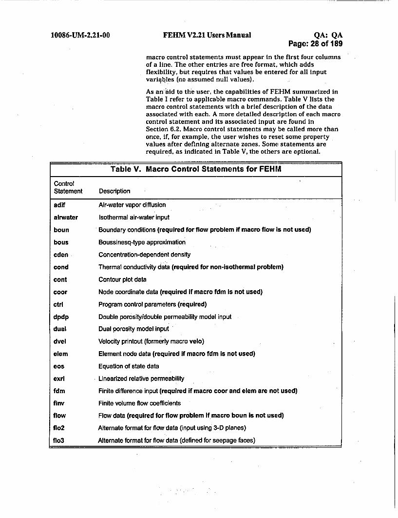
macro control statements must appear in the first four columnsof a line. The other entries are free format, which addsflexibility, but requires that values be entered for all inputvariqbles (no assumed null values).
As an aid to the user, the capabilities of FEiHM summarized inTable I refer to applicable macro commands. Table V lists themacro control statements with a brief description of the dataassociated with each. A more detailed description of each macrocontrol statement and its associated input are found inSection 6.2. Macro control statements may be called more thanonce, if, for example, the user wishes to reset some propertyvalues after defining alternate zones. Some statements arerequired, as indicated in Table V, the others are optional.
Table V. Macro Control Statements for FEHM
ControlStatement Description
adif Air-water vapor diffusion
airwater Isothermal air-water input
boun Boundary conditions (required for flow problem if macro flow Is not used)
bous Boussinesq-type approximation
cden Concentration-dependent density
cond Thermal conductivity data (required for non-isothermal problem)
cont Contour plot data
coor Node coordinate data (required If macro fdm Is not used)
ctrl Program control parameters (required)
dpdp Double porosity/double permeability model input
dual Dual porosity model input
dvel Velocity printout (formerly macro velo)
elem Element node data (required if macro fdm Is not used)
eos Equation of state data
exrl Linearized relative permeability
fdm Finite difference input (required if macro coor and elem are not used)
finv Finite volume flow coefficients
flow Flow data (required for flow problem If macro boun Is not used)
flo2 Alternate format for flow data (input using 3-D planes)
flo3 Alternate format for flow data (defined for seepage faces)

10086-UM-2.21-OO FEHIM V2.21 Users Manual QA: QAPage: 29 of 189
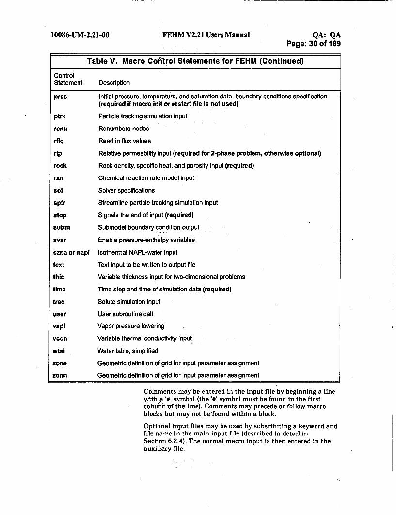
Table V. Macro Control Statements for FEHM (Continued)
ControlStatement Description
floafixo
flxz
fper
frlp
gdpm
grad
head
hflx
hyco
Ice or meth
impf
init
Isot
Iter
l1fc
Itup
lupk
mdnode
mptr
ngas
nobr
node
nod2
nod3
perm
pest
ppor
Alternate format for flow data (additive to previous flow definition)
Flux printout
Total flux through a zone printout
Permeability scaling factors
Relative permeability factors for residual air effect
Generalized dual porosity model
Gradient model input
Hydraulic head values
Heat flux input
Hydraulic conductivity input (required If macro perm Is not used)
Ice phase calculations (untested)
Time step control based on maximum allowed variable change
Initial value data (required If macro pres or restart file is not used)
Isotropic definition of control volume/finite element coefficients
Iteration parameters
Flow and transport between zone interfaces
Iterations used with upwinding
Upwind transmissibility including intrinsic permeability
Enables extra connections to be made to nodes
Multiple species partidc tracking simulation Input
Noncondensible gas (air) data
Don't break connection between nodes with boundary conditions
Node numbers for output and time histories
Node numbers for output and time histories, and alternate nodes for terminal output
Node numbers for output and time histories, alternate nodes for terminal output, andalternate nodes for variable porosity model information
Permeability input (required If macro hyco Is not used)
Parameter estimation routine output
Pressure and temperature dependent porosity and permeability
10086-UM-2.21-00 FEHM V2.21 Users Manual QA: QAPage: 30 of 189
Table V. Macro Coh'trol Statements for FEHM (Continued)
ControlStatement Description
pres
ptrk
renu
rflo
rip
rock
rxn
sol
sptr
stop
subm
svar
szna or napl
text
thic
time
trac
user
vapl
vcon
wtsi
zone
zonn
Initial pressure, temperature, and saturation data, boundary conditions specification
(required if macro init or restart file Is not used)
Particle tracking simulation input
Renumbers nodes
Read in flux values
Relative permeability input (required for 2-phase problem, otherwise optional)
Rock density, specific heat, and porosity input (required)
Chemical reaction rate model input
Solver specifications
Streamline particle tracking simulation input
Signals the end of input (required)
Submodel boundary c•ndition output
Enable pressure-enthalpy variables
Isothermal NAPL-water input
Text input to be written to output file
Variable thickness input for two-dimensional problems
Time step and time of simulation data (required)
Solute simulation input
User subroutine call
Vapor pressure lowering
Variable thermal conductivity input
Water table, simplified
Geometric definition of grid for input parameter assignment
Geometric definition of grid for input parameter assignment
Comments may be entered in the input file by beginning a linewith a '#' symbol (the '#' symbol must be found in the firstcolumn of the line). Comments may precede or follow macroblocks but may not be found within a block.
Optional input files may be used by substituting a keyword andfile name in the main input file (described in detail inSection 6.2.4). The normal macro input is then entered in theauxiliary file.

10086-UM-2.21-00 FEHM V2.21 Users Manual QA: QAPage: 31 of 189
Many input parameters such as porosity or permeability varythroughout the grid and need to have different values assignedat different nodes. This is accomplished in two ways. The firstuses a nodal loop-type definition (which is the default):
JA, JB, JC, PROP1, PROP2.
where
JA -first node to be assigned with the properties PROP 1,_PROP2,...
JB -last node to be assigned with the properties PROP 1,PROP2 ....
JC -loop increment for assigning properties PROPI, PROP2,
PROPI, PROP2, etc. - property values to be assigned to theindicated nodes.
In the input blocks using this structure, one or more propertiesare manually entered in the above structure. When a blank lineis entered, that input block is terminated and the code proceedsto the next group or control statement. (Note that blank inputlines are shaded in the examples shown in Section 6.2.) Thenodal definition above is useful in simple geometries where thenode numbers are easily found. Boundary nodes often come atregular node intervals and the increment counter JC can beadjusted so the boundary conditions are easily entered. To setthe same property values at every node, the user may set JAand JC to 1 and JB to the total number of nodes, oralternatively set JA = 1, and JB = JC = 0.
For dual porosity problems, which have three sets of parametervalues at any nodal position, nodes I to N [where N is the totalnumber of nodes in the grid (see macro coor)] represent thefracture nodes, nodes N + 1 to 2N are generated for the secondset of nodes, the first matrix material, and nodes 2N + I to 3Nfor the third set of nodes, the second matrix material. Fordouble porosity/double permeability problems, which have twosets of parameter values at any nodal position, nodes 1 to Nrepresent the fracture nodes and nodes N + 1 to 2N aregenerated for the matrix material.
For more complicated geometries, such as 3-D grids, the nodenumbers are often difficult to determine. Here a geometricdescription is preferred. To enable the geometric description thezone control statement (page 145) is used in the input filebefore the other property macro statements occur. The inputmacro zone requires the specification of the coordinates of 4-node parallelograms for 2-D problems or 8-node polyhedrons in3-D. In one usage of the control statement zone all the nodesare placed in geometric zones and assigned an identifyingnumber. This number is then addressed in the property inputmacro commands by specifying a JA < 0 in the definition of theloop parameters given above. For example if JA = -1, the

10086-UM-2.21-00 FEIIM V2.21 Users Manual QA: QAPage: 32 of 189
properties defined on the input line would be assigned to thenodes'defined as belonging to geometric Zone 1 (JB and JCmust be input but are ignored in this case), The controlstatement zone may be called multiple times to redefinegeometric groupings for subsequent input. The previous zonedefinitions are not retained between calls. Up to 1000 zones maybe defined. For dual porosity problems, which have three sets ofparameter values at any nodal position, Zone ZONEDPADD + Iis the default zone number for the second set of nodes defined by
Zone I, and Zone 2*ZONEDPADD + I is the default zonenumber for the third set of nodes defined by Zone I. For doubleporosity/double permeability problems, which have two sets ofparameter values at any nodal position, Zone ZONE_DPADD + Iis the default zone number for the second set of nodes defined byZone I. The value of ZONEDPADD Is determined by thenumber of zones that have been defined for the problem. If lessthan 100 zones have been used ZONEDPADD is set to 100,otherwise it is set to 1000. Zones of matrix nodes may also bedefined independently if desired.
Alternatively, the zonn control statement (page 148) may beused for geometric descriptions. Regions are defined the same asfor control statement zone except that previous zone definitionsare r.etained between calls unless specifically overwritten.
6.1.1.4 GoldSim InterfaceTo interface with GoldSim, FEHM is compiled as a dynamic linklibrary (DLL) subroutine that is called by the GoldSim code.When FEHM is called as a subroutine from GoldSim, theGoldSim software controls the time step of the simulation, andduring each call, the transport step is carried out and theresults passed back to GoldSim for processing and/or use asradionuclide mass input to another portion of the GoldSimsystem, such as a saturated zone transport submodel. Theinterface version of FEHM is set up only to perform particletracking simulations of radionuclide transport, and is notintended to provide a comprehensive flow and transportsimulation capability for GoldSim. Information concerning theGoldSim user interface may be found in the GoldSimdocumentation (Golder Associates, 2002).
6.1.2 Consecutive Cases
Consecutive cases can be run using the multiple realizations simulationoption (see Section 6.1.1.2 on page 27). The program retains only thegeometric information between runs (i.e., the grid and coefficientinformation). The values of all other variables are reinitialized with eachrun, either frorrr the input files or a restart file when used.
6.1.3 Defaults
Default values are set during the initialization process if overriding inputis not provided by the user.

10086-UM-2.21-00 FEHM V2.21 Users Manual QA: QAPage: 33 of 189
6.2 Individual Input Records or ParametersOther than the information provided through the control file or terminal I/O andthe multiple realization simulations file, the main user input is provided usingmacro control statements in the input file, geometry data file, zone data file, andoptional input files. Data provided in the input files is entered in free format withthe exception of the macro control statements and keywords which must appear inthe first four (or more) columns of a line. Data values may be separated withspaces, commas, or tabs. The primary input file differs from the others in that itbegins with a title line (80 characters maximum) followed by input in the form ofthe macro commands. Each file containing multiple macro commands should beterminated with the stop control statement. In the examples provided in thefollowing subsections, blank input lines are depicted with shading.
6.2.1 Control File or Terminal 1/0 Input
The parameters enumerated below, are entered in order one per line in thecontrol file (excluding the control file name [nmfile(l)]) or in response to aprompt during terminal input. If there is a control file, with the namefehmn.files in your local space (current working directory), FEHM willexecute using that control file and there will be no prompts. If anothername is used for the control file, it can be entered at the first prompt.
A blank line can be entered in the control file for any auxiliary files notrequired, for the "none" option for tty output, and for the "0" option for theuser subroutine number. The code will always write an input check file anda restart file, so if names are not provided by the user the defaults will beused. If an output file name is not specified, the generalized output iswritten to the terminal. File names that do not include a directory orsubdirectory name, will be located in the current working directory. Thedata files are described in more detail in Section 5.0.
Input Opt/ , Default DescriptionVariable Format Req
nmfil(1) character*100 Opt fehmn.files Control file name (this line is not included in
the control file)
nmfil( 2) character*100 Req fehmn.dat Main input file name
nmfil( 3) character*100 Opt not used Geometry data input file name
nmfil(4) character*100 Opt not used Zone data input file name
nmfil( 5) character*100 Opt terminal Main output file name
nmfil( 6) character*100 Opt not used Restart input file name
nmfil( 7) character*100 Opt fehmn.fin Restart output file name
nmfil( 8) character*100 Opt not used Simulation history output file name
nmfil( 9) character*100 Opt not used Solute history output file name
nmfil(10) character*100 Opt not used Contour plot output file name. (Required ifusing avs option in cont macro.)
r,-

10086-UM-2.21-00 FEHM V2.21 Users Manual QA: QAPage: 34 of 189
Input Format Default DescriptionVariable Req
nmfil(1 1) character*100 Opt not used Dual porosity or double porosity I doublepermeability contour plot output file name
nmfil(12) character*100 Opt not used Coefficient storage file name
nmfil(13) character*100 Opt fehmn.chk Input check output file name
tty.lag character*4 Opt none Terminal output flag: all, some, none
usubnum integer Opt 0 User subroutine call number
The following are two examples of input control files. In the example on theleft, all input will be found in the current working directory and outputfiles will also be written to that directory. The blank lines indicate thatthere is no restart initialization file, the restart output file will use thedefault file name (fehmn.fin), a dual porosity contour plot file is notrequired, and the coefficient storage file is not used. The *some" keywordindicates that selected information is output to the terminal. The ending"0" indicates that the user subroutine will not be called. In the example onthe right, input will be found in the "groupdir" directory, while output willbe written to the current working directory. The 'none" keyword indicatesthat no information should be written to the terminal.
Files *fehmn.files":
tape5.dat Igroupdir/c14-3tape5.dat Igroupdir/grid-402tape5.dat /groupdir/c14-3tape5.out c14-3.out
Igroupdir/cl4-3.inic14-3.fin
tape5.his c14-3.histape5.trc c14-3.trctape 5.con c14-3.con
c14-3.dpc14-3.stor
tape5.chk c14-3.chksome none0 0
6.2.2 Multiple Realization Simulations Input
The multiple realization simulations input file (fehmn. msim) contains thenumber of simulations to be performed and, on UNIX systems, instructionsfor pre- and post-processing input and output data during a multiplerealization simulation. The file uses the following input format:
Line I nsim
Lines 2-N single-line
In the following example, 100 simulations are performed with pre and post-processing steps carried out. The first line after the number of simulationsdemonstrates how the current and total number of simulations can be

10086-UM-2.21-00 FEHM V2.21 Users Manual QA: QAPage: 35 of 189
InputVariable Format
integer
Description
nsim Numberiof simulation realizations to be performed
single-line character*80 An arbitrary number of lines of UNIX shell script style instructions:lines 2-n: lines which are written to a file called fehmn.pre, which is
invoked as a shell script (UNIX systems) that is performed before eachrealization using the following command: sh fehmn.pre $1 $2
line n+1: the keyword 'post', placed in the first four columns of the inputfile, denotes that the previous line is the last line in the fehmn.prescript, and that the data for the post-processing script fehmn.postfollows
lines n+2 to N: lines which are written to a file called fehmn.post, whichis invoked as a shell script (UNIX systems) that is performed aftereach realization using the following command: sh fehmn.post $1 $2
Thus, the files fehmn.pre and fehmn.post are created by the code and aremeant to provide the capability to perform complex pre- and post-processing steps during a multiple realization simulation. Scriptarguments $1 and $2 represent the current simulation number and nsim,the total number of simulations, respectively.
accessed in the fehmn.pre shell script. This line will write the following
output for the first realization:
This is run number 1 of 100
The pre-processing steps in this example are to remove the fehmn.files filefrom the working directory, copy a control file to fehmn.files, copy aparticle tracking macro input file to a commonly named file calledptrk.input, and write a message to the screen. The fehmn.files files shouldbe used or else the code will require screen input of the control file namefor every realization. One hundred particle tracking input files would havebeen generated previously, and would have the names ptrk. npl, ptrk.np2,
ptrk.np100. Presumably, these files would all have different transportparameters, resultingkin 100 different transport realizations. The post-processing steps involve executing a post-processor program for the results(processl-fuj). This post-processor code generates an output file calledresults.output, which the script changes to npl.output, np2.output,...,nplOO.output, for further processing after the simulation.:
One other point to note is that the variable *curnum" in this example:isdefined twice, once in the pre-processor and again in the post-ýprocessor.This is necessary because fehmn.pre and fehmn.post are distinct shellscripts that do not communicate with one another.
-V.-

10086-UM-2.21-00 FEHM V2.21 Users Manual QA: QAPage: 36 of 189
File "fehmn.msim":
100echo This is run number $1 of $2rm fehmn.filescurnum='expr $1'cp control.run fehmn.filesrm ptrk.inputcp ptrk.np$curnum ptrk.inputecho starting up the runpostcurnum=*expr $1V/home/robinson/fehmlchunjli/ptrk/processl_jujrm np$curnumoutputmv results.output np$curnum.outputecho finishing the run again
6.2.3 Transfer function curve data Input file
In the FEHM particle tracking models, diffusion of solute from primaryporosity into the porous matrix is captured using an upscaling proceduredesigned to capture the small scale behavior within the field scale model.The method is to impart a delay to each particle relative to that of anondiffusing solute. Each particle delay is computed probabilisticallythrough the use of transfer functions. A transfer function represents thesolution to the transport of an idealized system with matrix diffusion at thesub-grid-block scale. After setting up the idealized model geometry of thematrix diffusion system, a model curve for the cumulative distribution oftravel times through the small-scale model is computed, either from ananalytical or numerical solution. Then, this probability distribution is usedto determine, for each particle passing through a given large-scale gridblock, the travel time of a given particle. Sampling from the distributioncomputed from the small scale model ensures that when a large number ofparticles pass through a cell, the desired distribution of travel timesthrough the model is reproduced. In FEHM, there are equivalentcontinuum and dual permeability formulations for the model, each of whichcall for a different set of sub-grid-block transfer function curves. Thesecurves are numerical input to the FEHM, with a data structure describedbelow. Optional iniput in macros mptr, ptrk, and sptr is used to tell thecode when transfer function curves are required and whether 2 or 3(numparams) parameter curves are to be used.
Input Variable Format Description
DUMMY-STRING character*4 If keyword "free" is input at the beginning of the file, the codeassumes an irregular distribution of transfer functionparameters and performs either a nearest neighbor search tochoose the transfer function curve, or a more computationallyintensive multi-curve interpolation.
NCURVES integer Total number of transfer function curves input in the file whenkeyword "free" is used.
10086-UM-2.21-OO FEHM V2.21 Users Manual QA: QAPage: 37 of 189
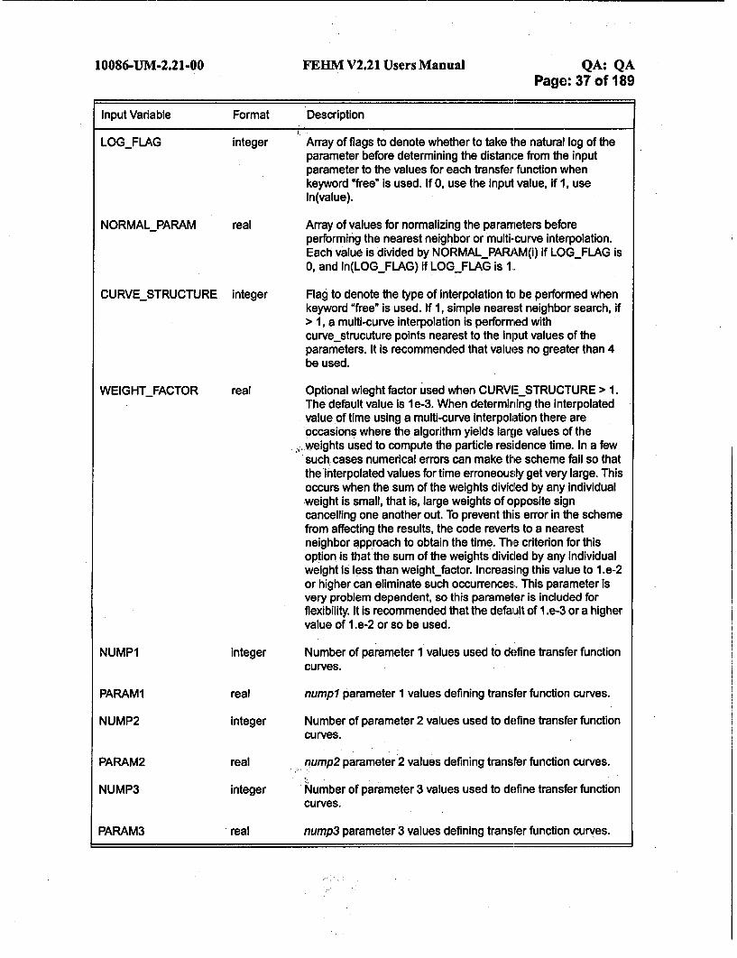
Input Variable Format Description
LOGFLAG
NORMALPARAM
integer
real
CURVESTRUCTURE integer
WEIGHTFACTOR real
Array of flags to denote whether to take the natural log of theparameter before determining the distance from the inputparameter to the values for each transfer function whenkeyword "free" is used. If 0, use the Input value, if 1, useIn(value).
Array of values for normalizing the parameters beforeperforming the nearest neighbor or multi-curve interpolation.Each value is divided by NORMALPARAM(i) if LOGFLAG is0, and In(LOGFLAG) if LOG-FLAG is 1..
Flag to denote the type of interpolation to be performed whenkeyword *free" is used. If 1, simple nearest neighbor search, if> 1, a multi-curve interpolation is performed withcurve strucuture points nearest to the input values of theparameters. It is recommended that values no greater than 4be used.
Optional wieght factor used when CURVESTRUCTURE > 1.The default value is le-3. When determining the interpolatedvalue of time using a multi-curve interpolation there areoccasions where the algorithm yields large values of the
,,.weights used to compute the particle residence time. In a fewsuch cases numerical errors can make the scheme fail so thatthe interpolated values for time erroneously get very large. Thisoccurs when the sum of the weights divided by any individual-weight is small, that is, large weights of opposite signcancelling one another out. To prevent this error in the schemefrom affecting the results, the code reverts to a nearestneighbor approach to obtain the time. The criterion for thisoption is that the sum of the weights divided by any individualweight is less than weightjfactor. Increasing this value to 1.e-2or higher can eliminate such occurrences. This parameter isvery problem dependent, so this parameter is included forflexibility. It is recommended that the default of 1 .e-3 or a highervalue of 1 .e-2 or so be used.
Number of parameter 1 values used to define transfer function
curves.
numpl parameter 1 values defining transfer function curves.
Number of parameter 2 values used to define transfer functioncurves.
nump2 parameter 2 values defining transfer function curves.
Number of parameter 3 values used to define transfer functioncurves.
nump3 parameter 3 values defining transfer function curves.
NUMP1
PARAM1
NUMP2
PARAM2
NUMP3
integer
real
integer
real
integer
PARAM3 real

10086-UM-2.21-00 FEHM V2.21 Users Manual QA: QAPage: 38 of 189
Input Variable Format Description
D4 integer Fracture-matrix flow interaction flag (d4 = 1, 4). For the three-parameter option, the dual permeability model requires fourtransfer function curves for each set of parameters. Interactionscan occur from fracture-fracture (d4=1), fracture-matrix (d4=2),matrix-fracture (d4=3), and matrix-matrix (d4=4).
NUMPMAX integer Maximum number of delay time and concentration values fortransfer function curves.
NUMP integer Number of delay time and concentration values in each transferfunction curve (numpl, numpZ nump3, d4).
DTIME real Transfer function curve delay times (numpI, numpZ nump3,d4, nump).
CONC real Transfer function curve concentrations (numpl, nump2,nump3, d4, nump).
OUTPUTFLAG character*3 If optional keyword *out" is entered at the end of the file thecode outputs information on the parameter space encounteredduring the simulation in the *.out file. See "mptr" macro forfurther discusion of the output option.
The transfer function curve data file uses the following format if a regulargrid of parameters is input. Please note that parameter values for thisformat should be input from smallest to largest value:
numplparaml (I), I = I to numplnump2param2 0), j = 1 to nump2If 2 parameter curves are being input
numpmaxFor each i,j (nump3 =l, d4 = 1)nump(i,J, 1, 1), paraml(i), param2j)followed by for each nump(i, J, 1. 1)time(i, J, 1, 1, nump), conc(i, J 1, 1, nump)
Or if 3 parameter curves are being inputnump3param3(k), k 1 to nump3nump.maxFor each d4, i, J, knump(i, J, k, d4), paraml(i), param2(), param3(k), d4followed by for each nump(l, J, k, d4)time(i, J, k, d4, nump), conc(i, J, k, d4, nump)
out-flag (optional) - keyword "out"
10086-UM-2.21-00 FEHM V2.21 Users Manual QA: QAPage: 39 of 189
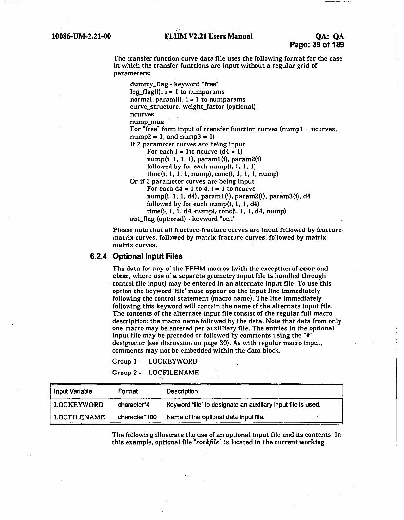
The transfer function curve data file uses the following format for the casein which the transfer functions are input without a regular grid ofparameters:
dummy-flag - keyword "free"log_flag(i), I = I to numparamsnormal-param(i), I = 1 to numparamscurvestructure, weightjactor (optional)ncurvesnump.maxFor "free" form input of transfer function curves (numpi I ncurves,nump2 = 1, and nump3 = 1)If 2 parameter curves are being input
For each i = Ito ncurve (d4 = 1)nump(i, 1, 1, 1), paraml (I), param2(i)followed by for each nump(i, 1, 1, 1)time(i, 1, 1, 1, nump), conc(i, 1, 1, 1, nump)
Or if 3 parameter curves are being inputFor each d4 1 to 4, j = 1 to ncurvenump(i, 1, 1, d4), paramI (I), param2(1), param3(i), d4followed by for each nump(i, 1, 1, d4)time(i., 1, 1, d4, nump),• conc(i, 1, 1, d4l, hump)
out_flag (optional) - keyword "out"
Please note that all fracture-fracture curves are input followed by fracture-matrix curves, followed by matrix-fracture curves, followed by matrix-matrix curves.
6.2.4 Optional Input Files
The data for any of the FEHM macros (with the exception of coor andelem, where use of a separate geometry input file is handled throughcontrol file input) may be entered in an alternate input file. To use thisoption the keyword 'file' must appear on the input line immediatelyfollowing the control statement (macro name). The line immediatelyfollowing this keyword will contain the name of the alternate input file.The contents of the alternate input file consist of the regular full macrodescription: the macro name followed by the data. Note that data from onlyone macro may be entered per auxilliary file. The entries in the optionalinput file may be preceded or followed by comments using the W#"designator (see discussion on page 30). As with regular macro input,comments may not be embedded within the data block.
Group 1 - LOCKEYWORD
Group 2 - LOCFILENAME
Input Variable Format Description
LOCKEYWORD character*4 Keyword 'file' to designate an auxiliary input file is used.
LOCFILENAME character*100 Name of the optional data input file.
The following illustrate the use of an optional input file and its contents. Inthis example, optional file "rockfile" is located in the current working

10086-UM-2.21-OO FEHM V2.21 Users Manual QA: QAPage: 40 of 189
directory. Input for macro "rock" is described in Section 6.2.58 onpage 104.
file
rockfile
File "rockfile":
6.2.5 Control statement adif (optional)
Air-water vapor diffusion. The air-water diffusion equation is given asEquation (21) of the "Models and Methods Summary" of the FEHMApplication (Zyvoloski et al. 1999).
Group I- TORT
Input Variable Format Description
TORT real Tortuosity for air-water vapor diffusion.If TORT > 0, r of eqn 21, otherwise
If TORT < 0, abs(¶4Sv) of the same equation.
The following Is an example of adif. In this example the tortuosity (r) forvapor diffusion Is specified to be 0.8.
adif 0.8 [,
6.2.6 Control statement airwater (optional)
Isothermal air-water two-phase simulation.
Group 1 - ICO2D
Group 2 - TREF, PREF
Input Variable Format Description
ICO2D integer Determines the type of air module used.ICO2D = 1, 1 degree of freedom solution to the saturated-unsaturated
problem Is produced. This fbrmulation is similar to the Richard'sEquation.
ICO2D = 2, 1 degree of freedom solution is obtained assuming onlygas flow with no liquid present.
ICO2D = 3, full 2 degree of freedom solution.All other values are ignored. The default is 3.

10086-UM-2.21-00 FEHM V2.21 Users Manual QA: QAPage: 41 of 189
Input Variable Format Description
TREF real Reference temperature for properties (*C).
PREF real Reference pressure for properties (MPa).
Several macros are affected if the air module is enabled. These are
pres - Because the air-water formulation is 2-phase at all times, careshould be taken to insure that IEOSD is always specified to be2. Likewise, saturations (not temperatures) are used.
lnit - This macro should not be used because the saturation valuescannot be specified.
flow - A variety of different flow and boundary values are input withthis macro when the macro airwater is also used. Seedescription of control statement flow.
The following is an example of airwater. In this example, a full 2-degrees-of-freedom solution is specified with a reference temperature for propertyevaluation of 20 'C and a reference pressure of 0.1 MPa.
airwater31320. 0.1
6.2.7 Control statement boun (either boun or flow is required for a flowproblem)Implement boundary conditions and sources or sinks. Input may be timedependent and cyclic. Time step sizes may also be adjusted.
Group 1 - KEYWORD
The Group 1 KEYWORD 'model', which starts each model sequence, isfollowed immediately by a Group 2 KEYWORD of 'ti' or 'cy'.
Group 2 - KEYWORD
Group 3 - NTIMES, TIME(I), I=1,NTIMES
The Group 4 KEYWORDs define the various boundary conditionparameters being entered. These KEYWORDs and associated data, Group5, are repeated as needed for each model.
Group 4 - KEYWORD
Group 5 - VARIABLE(I), I=I,NTIMES
Additional models are entered by beginning again with Group 1. TheMODEL-NUMBER is incremented each time a new model is read, and isused to assign boundary conditions to specified nodes or zones in Group 6..After all models have been entered, the section is terminated withKEYWORD 'end' or a blank line.
Group 6 -JA, JB, JC, MODELNUMBER (JA, JB, JC-defined on page 31)
The following is an example of boun. In this example two models aredefined. The first model cyclically changes the water source in a 1.e05 daycycle, i.e., the 'cy' keyword entry shows that the time cycle ends at l.e05

10086-UM-2.21-00 FEHM V2.21 Users Manual QA: QAPage: 42 of 189
Input Variable Format Description
KEYWORD character*4 Keyword specifying a model designation, time for boundary conditionor source/sink changes, or actual variable or source change.Keywords, which must be entered starting in the first column, are:
model - new model definition to follow
Note: Descriptive text, such as the model number, may beappended after the 'model' keyword as long as it is containedon a single line, and begins after column four.
ti - time sequence for changes to follow (days)cy - cyclic time sequence for changes to follow (days)
Note: The keywords, 'ti' and 'cy', require the time to start at 0.0.This provides the initial boundary and source/sink information.If the input for 'ti' or 'cy' does not start at 0.0 time the codeassumes boundary conditions and source/sinks are 0.0 attime 0.0. The 'cy' keyword involves a cyclic changing ofconditions. In our procedure the cycle ends at the lastspecified time. Thus the code reverts to the first specified timevalues. Because of this, the boundary conditions and source/sinks for the last time change are always set to the first timevalues.
sa - air source sequence for changes to follow (kg/s)sw - water source sequence for changes to follow (kg/s)swf - source water factor sequence for changes to follow
(multiplier for existing flux)se - enthalpy source sequence for changes to follow (MW)sf - water seepage face sequence with pressures for changes to
follow (MPa)sfh - water seepage face sequence with heads for changes to
follow (m)fd - water drainage area sequence for changes to follow (m2 )
dsa - distributed air source sequence for changes to follow (kg/s)dsw - distributed water source sequence for changes to follow
,(kg/s)dse - distributed enthalpy source sequence! for changes to follow
(MW)Note: A distributed source (keywords 'dsa', 'dsw', and 'dse') isa source term divided over a group of nodes or a zoneproportional to the nodal volume.
s - fixed saturation sequence for changes to followhd - fixed hydraulic head sequence for changes to follow (m)pw - fixed water pressure sequence for changes to follow (MPa)pa - fixed air pressure sequence for changes to follow (MPa)hdo - fixed hydraulic head sequence for changes to follow (m)
(constrained to outflow only)pwo - fixed water pressure sequence for changes to follow (MPa)
(constrained to outflow only)pao., - fixed air pressure sequence for changes to follow (MPa)
(constrained to outflow only)

10086-UM-2.21-OO FEHIM V2.21 Users Manual QA: QAPage: 43 of 189
Input Variable Format Description
en - fixed enthalpy sequence for changes to follow (MW)
t - fixed temperature sequence for changes to follow (CC)h - fixed humidity sequence for changes to follow (must be used
with van Genuchten relative permeability model)ft - fixed flowing temperature sequence for change to follow
(°C). By flowing temperature we mean the temperature ofthe inflow stream for a specified source. If no influx sourceoccurs where this condition is applied, it will be ignored.
if - impedance factor for use with fixed water pressure boundarycondition. If left out the impedance factor will be set to thevolume of the grid cell.
si - initial value saturation sequence for changes to followpa• - initial value air pressure sequence for changes to follow
(MPa)pwi - initial value water pressure sequence for changes to follow
(MPa)tmi - initial value temperature sequence for changes to follow (0C)
Note: The keywords 'si', 'pai', 'pwi', and 'tmi' refer to changesfor a variable that is NOT fixed. They are similar to specifyinginitial conditions in that regard but may be changed accordingto a time sequence. At present these 4 keywords only workwith isothermal air-water calculations.
NTIMES
TIMEVARIABLEMODEL-NUMBER
chmo - model number sequence for changes to followts - timestep sequence for changes to follow (days)end - signifies end of keyword input, a blank line will also work.
integer Number of time changes for boundary condition or source/sinkspecification.
real NTIMES times for changes in boundary conditions or source/sinks.real NTIMES new values for boundary conditions or source/sinks.integer Boundary condition model to be associated with designated nodes or
zones (the number corresponds to the numerical order in which themodels were input, i.e., beginning with KEYWORD 'model')
days and at this time the cycle reverts to 0.0 days. Note that the watersource at 1.e05 days equals that at 0.0 days. Also in model 1 the flowingtemperature was alternated between 200C and 500C. The second modeluses a time change that occurs at 1.e20 days. This effectively removes anytime variance from model 2. Model 2 has a fixed water pressure and flowingtemperature condition. The models are applied at nodes 26 and 27 in thelast two lines. It should be noted that the model numbers included in theexample (following KEYWORD 'model') are not part of' the required inputbut are descriptive text used to enhance readability of the macro.

10086-UM-2.21-00 FERM V2.21 Users Manual QA: QAPage: 44 of 189
Dounmodel Icy
4 0.0 1.el 1.e2 1.e5sw
-1.e-4 -1.e-5 -1.e-3 -1.e-4ft
20.0 50.0 50.0 20.0model 2ti
2 0.0 1 .e20pw
0.1 0.1ft
20.0 20.0end
26 26 1 127 27 1 2
6.2.8 Control statement bous (optional)
Constant density and viscosity are used for the flow terms (Boussinesqapproximation). NOTE: where the bous macro is used, the gravity term inthe air phase is set to zero.
Group I - ICONS
Input Variable Format Description
ICONS integer Parameter to enable constant density and viscosity for flow termsICONS •0 enabled.ICONS =0 disabled (default).
The following is an example of bous. In this example the Boussinesqapproximation is enabled.b0ou s
6.2.9 Control statement cdenUse concentration-dependent density for flow.
The following restrictions apply to the use of this macro: •) It cannot beused with the macro *head", which assumes constant fluid density; 2) Theupdating of density is explicit, based on the concentrption values at theprevious time step. Therefore, accuracy of the solution. :must be tested byusing a smaller time step and ensuring that the results h ve converged; 3)The fluid flow time steps should be small enough that oanl one or twosolute time steps'are carried out before the next fluid titt step, becauserelatively small changes in the concentration field are: required foraccuracy; and 4) The heat and mass transfer solution must be kept onduring the entire simulation for the results to be meaningful (see macrotrac).

10086-UM-2.21-00 FEHM V2.21 Users Manual QA: QAPage: 45 of 189
Group 1 -
Group 2 -
ISPCDEN
FACTCDEN
Input Variable Format Description
ISPCDEN integer The number of the chemical component in trac that is used forapplying the concentration-dependent density.
FACTCDEN real The factor used in the following relationship for fluid density (kg/m 3):
density = density water + FACTCDEN*Cwhere densitywater= the density of pure water (kg/m3 ), and C isthe concentration of chemical component ISPCDEN
The following is an example of cden. In this example, component number 1in trac is used. For concentrations of order 1, the density correction wouldbe 100, of order 10% of the nominal value of water density of 1000 kg/m3 .
cden1
100.
6.2.10 Control statement cond (required for non-isothermal problem)
Assign thermal conductivities of the rock.
Group 1 - JA, JB, JC, THXD, THYD, THZD (JA, JB, JC - defined onpage 31)
Input Variable Format Default Description
THXD real 1.e-30 Thermal conductivity in the x-direction ( .
THYD real 1 .e30 Thermal conductivity In the y-cirection ( mWK
THZD real 1.e-30 Thermal conductivity in the zy-irection ( .
The following is an example of cond. In this example all the nodes
numbered I through 140 have thermal conductivities of ( m K) in the X
and Y directions, and 0 in the Z direction.
Scond
1 140 1 1.00e-00 1.00e-00 O.OOe-00
6.2.11 Control statement cont (optional)Contour data output format, output timestep Intervals, and time intervals.
Group I - NCNTR, CONTIM

10086-UM-2.21-00 FEHM V2.21 Users Manual QA: QAPage: 46 of 189
An alternative form of input for macro cont is possible. This is
Group I - ALTC, NCNTR, CONTIM, KEYWORD
Group 2 - CHDUM (only Input if ALTC is 'avs' or 'avsx')
-or-
Group 2 - NSURF, IZONEISURF(I), I=l, NSURF (only input if ALTC is'sur' or 'tec')
Input Variable Format Description
ALTC character*4 Keyword specifying the type of contour output wanted (avs, avsx,fehm, free, ment, ptrn):
'avs' produces contour plot files compatible with the AVSpostprocessor.
'avsx' produces contour plot files compatible with the AVS Expresspostprocessor.
'fehm' produces a binary output file. The same contour plot file isproduced using the first form of Group1 Input.
'free' produces a free format contour plot file.'mernt' produces a contour plot file compatible with the MENTAT
postprocessor.'ptrn' produces a contour plot file compatible with the PATRAN
postprocessor.'sur' produces a contour plot file compatible with the SURFER
postprocessor.'tec' produces a contour plot file compatible with the TECPLOT
postprocessor.
NCNTR integer Time step interval for contour plots (number of timesteps). Outputcontour information each NCNTR timesteps.
CONTIM real Time interval for contour plots (days). In addition to output eachNCNTR timesteps, output contour information each CONTIM days.
KEYWORD character*4 Optional keyword 'time", use time (days) in file name instead ofnumber (used when altc is "avs" or "avsx" or ?"sur" or "tec")
NSURF integer Number of output zones used when aftc is "suro or "tec"
IZONESURF integer List of nsurf zone numbers used when altc is "sur" or "tec"
CHDUM character*72 Keyword specifying type of AVS contour plot data files to be createdin AýVS UCD or AVS Express format. Keywords are entered one perline and terminated with 'endavs'. Valid keywords (case insensitive)are:
(m)aterial - output contour values for material properties.(I)iquid - output contour values for liquid phase.(va)por - output contour values for vapor phase.(ve)locity - output velocity values.(dp)dp - output contour values for dual permeability nodes.(p)ressure - output pressure values.(h)ead - output head values.

10086-UM-2.21-00 FEHM V2.21 Users Manual QA: QA
Page: 47 of 189
Input Variable Format Description(tpemperature - output temperature values.
(s)aturation - output saturation values.(c)oncentration - output solute concentration values.(f)ormatted - output data in ASCII format.(e)ndavs - last keyword entered.
If a format keyword is not entered, the default is 'formatted'. In thecurrent version of the code this is the only format option supported.The default for data keywords is "off" (no output). The letters given in( ) are sufficient to identify the keyword.
FEHM will automatically distinguish between the alternative inputformats. When keywords are used they must be entered starting in the firstcolumn. The contour data will be output whenever either of the intervalcriteria are satisfied.
For AVS output, if the material keyword is selected, the following materialproperty values will be written for each node: permeability in the x, y, andz directions, thermal conductivity in the x, y, and z directions, porosity,rock specific heat, capillary pressure, relative permeability model beingused, and capillary pressure model being used. If vapor and/or liquid areselected, pressure or velocity must also be defined (otherwise, no data forthese values will be written), velocity will result in vector values, pressurevalues will be scalar. If concentration is selected, values will be output onlyif nspeci is defined for tracer solutions. See the control statement trac for adescription of nspeci for solutes.
The following are examples of cont. For the first example, FEHM binaryformat contour output files will be written every 100 timesteps and for each1.e20 days. The second example invokes AVS contour output. AVS UCDformatted files will be written for every 100 time steps and 1.e20 days. Theresulting files will include a log file, geometry file, plus header and datafiles for the following: material properties, solute concentrations, liquidvelocities, pressures and temperatures.
cont cont100 1.e20 avs 100 1.e20
matconliquidvelocitypressuretempformattedendavs
6.2.12 Control statement coor (required if macro fdm not used)
Node coordinate data. These data are usually created by a mesh generationprogram, then cut and copied into the input file or a separate geometrydata Input file. The mesh must be a right handed coordinate system. Notethat X, Y, and Z coordinates mustbe entered even if a problem is notthree-dimensional.

10086-UM-2.21-OO FEHM V2.21 Users Manual QA: QAPage: 48 of 189
Group I - N
Group 2 - MB, CORDI, CORD2, CORD3
To end the control section a blank line is entered.
Input Variable Format Description
N integer Number of nodes in the grid
MB integer Node number. If MB < 0 then the difference between the absolutevalue of MB and the previously read absolute value of MB is used togenerate intermediate values by interpolation.
CORD1 real X-coordinate of node MB (m).
CORD2 real Y-coordinate of node MB (m).
CORD3 real Z-coordinate of node MB (m).
The following is an example of coor. In this example, there are 140 nodesin the grid. Node number 1 has X, Y, Z coordinates of 0., 200., and 0. metersrespectively, node 2 has X, Y, Z coordinates of 12.5, 200., and 0. metersrespectively, and so forth, with node number 140 having X, Y, Z coordinatesof 300., 0., and 0. meters respectively.
coor140
1 0.00000 200.00000 0.000002 12.50000 200,00000 0.00000
10 212.50000 200.00000 0.00000
140 300.00000 0.00000 0.00000
6.2.13 Control statement ctrl (required)
Assign various control parameters needed for equation solvers and matrixsolver routines. Suggested values for the control parameters are shown in* (" in the table. For older input files where MAXSOLVE and ACCM werenot input, the default is ACCM = gmre and MAXSOLVE = 3*NORTH.
Group 1 - MAXIT, EPM, NORTH, MAXSOLVE, ACCM
Group 2 - JA, JB, JC, NAR (JA, JB, JC - defined on page 31)
Group 3 - AAW,,AGRAV, UPWGT
Group 4 - IAMM, AIAA, DAYMIN, DAYMAX
Group 5 - ICNL, LDA

10086-UM-2.21-00 FEHM V2.21 Users Manual QA: QAPage: 49 of 189
Input Variable Format Default Description
MAXIT integer Maximum number of iterations allowed in either the overallNewton cycle or the inner cycle to solve for the correctionsat each iteration. If MAXIT < 0 then the maximum number ofiterations is ABS(MAXIT) but the minimum number ofiterations is set to 2. (10)
EPM real Tolerance for Newton cycle (nonlinear equation tolerance).{1 .e-5)
NORTH integer Number of orthogonalizations in the linear equation solver." {8 for gmre, 1 for bcgs}
MAXSOLVE integer Maximum number of solver iterations allowed
ACCM character*4 Acceleration method for solvebcgs - Biconjugate gradient stabilized accelerationgmre - Generalized minimum residual acceleration
NAR integer 1 The order of partial Gauss elimination {1 or 2 isrecommended). Larger values increase memory utilizationbut may be necessary for convergence.
AAW real Implicitness factor. {1)AAW < 1, use standard pure implicit formulation.AAW > 1, use second-order implicit method.
AGRAV integer Direction of gravityAGRAV = 0, no gravity is used.AGRAV = 1, X-direction.AGRAV = 2, Y-direction.AGRAV = 3, Z-direction.
A value for gravity of 9.81 m/s 2 is used in the code whenAGRAV A 0. If AGRAV > 3, AGRAV is set equal to 3.
UPWGT real Value of upstream weighting {0.5 < UPWGT < 1.0).If UPWGT < 0.5, UPWGT is set to 0,5If UPWGT > 1.0, UPWGT is set to 1.0
IAMM integer Maximum number of iterations for which the code willmultiply the time step size. If this number of time steps isexceeded at any time, the time step will not be increased forthe next time {7-10}.
AIAA real 1 Time step multiplier {1.2-2.0)
DAYMIN real 1.0e-05 Minimum time step size (days)
DAYMAX real 30.0 Maximum time step size (days)DAYMAX real 30.0 Maximum time step size (days)

10086-UM-2.21-OO FEHM V2.21 Users Manual QA: QAPage: 50 of 189
Input Variable Format Default Description
ICNL integer Parameter that specifies the geometryICNL = 0, three-dimensionalICNL = 1, X - Y planeICNL = 2, X - Z planeICNL = 3, Y - Z planeICNL = 4, X - Y radial plane, (radius is X)ICNL = 5, X - Z radial plane, (radius is X)ICNL = 6, Y - Z radial plane, (radius is Y)
LDA integer 0 Parameter that specifies the external storage of geometriccoefficients
LDA = +2, element coefficients are read, unformatted, fromfile filen.stor and no coefficients are calculated in thecode
LDA = +1, element coefficients are read from file filen.storand no coefficients are calculated in the code
LDA = 0, element coefficients are cafculated in the codeand not saved
LDA = -1, element coefficients are calculated in the codeand saved on file filen.stor
LDA = -2, element coefficients are calculated in the codeand saved, unformatted, on file filen.stor
It should be noted that if the coefficients are read from a file(LDA = 1) then the macro finv is ignored as well asinformation read from macros elem and coor.
The following is an example of ctrl. In this example, the maximum numberof iterations allowed is 40, tolerance for solving the nonlinear equationsusing Newton iterations is l.e-7, and the number of orthogonalizations inthe linear equation solver is 8. The order of partial Gauss elimination forall nodes 1 through 140 Is 1. A forward implicit formulation is used for thetime derivative, there is no gravity, and full upstream weighting is used.The number of iterations for which the time step is increased is 40, thetime step is increased by a factor of 1.2 at each iteration, the minimumtime step size is 0.1 days, and the maximum time step size is 60 days. Thegeometry of the problem is 2-dimensional in the X-Y plane and the finiteelement coefficients are calculated during the run and not saved.
ctrl40 1 .e-7 8 24 gmre
1 140 1 1
1.0 0.0 1.040 1,2 0.1 60.0
1 0
6.2.14 Control statement dpdp (optional)
Double porosity / double permeability formulation. There are two sets ofparameter values at any nodal position, for which property values must bedefined. Nodes I to N (see macro coor for definition of N) represent thefracture nodes and nodes N + 1 to 2N the matrix material. When zones are

10086-UM-2.21-OO FEHM V2.21 Users Manual QA: QAPage: 51 of 189
used with the dpdp macro, additional zones are automatically generated.See instructions for the macro zone for a more detailed description. Thedpdp parameters are only defined for the first N nodes.
Group 1 - IDPDP
Group 2 - JA, JB, JC, VOLFD1 (JA, JB, JC - defined on page 31)
Group 3 - JA, JB, JC, APUVI (JA, JB, JC - defined on page 31)
Input Variable Format Default Description
IDPDP integer Solution descriptor for double porosity/doublepermeability solution.
IDPDP = 0, information is read but not used.IDPDP •0, dpdp solution is implemented.
VOLFD1 real 1. Volume fraction for fracture node.
APUV1 real 10. Length scale for matrix nodes (m).
The volume fraction VOLFD1 is related to the total volume by
VOLFD 1 + VOLFD2 = 1.0
where VOLFD2 is the volume fraction of the matrix node. If permeabilitymodel IRLP = 4 is selected in control statement rip, VOLFD1 is calculatedfrom RP15 (fracture porosity) in that control statement.
The following is an example of dpdp. In this example,, the dual porosity/permeability solution is implemented for all nodes from 1 through 140. Thefractional volume in the fractures (compared to the total volume) is 0.005and the length scale for matrix nodes is 0.1 m.
dpdp
1 140 1 0.005
1 140 1 0.10
6.2.15 Control statement dual (optional)
Dual porosity formulation. There are three sets of parameter values at anynodal position, for which property values must be defined. Nodes 1 to N(see macro coor for definition of N) represent the fracture nodes, nodesN + 1 to 2N the first matrix material, and nodes 2N + 1 to 3N the secondmatrix material. When zones are used with the dual macro, additionalzones are automatically generated. See instructions for the macro zone fora more detailed description. The dual parameters are only defined for thefirst N nodes.
Group 1 - IDUALP
Group 2 - JA, JB, JC, VOLFD1 (JA, JB, JC - defined on page 31)
Group 3 - JA, JB, JC, VOLFD2 (JA, JB, JC - defined on page 31)
Group 4 - JA, JB, JC, APUVD (JA, JB, JC - defined on page 31)
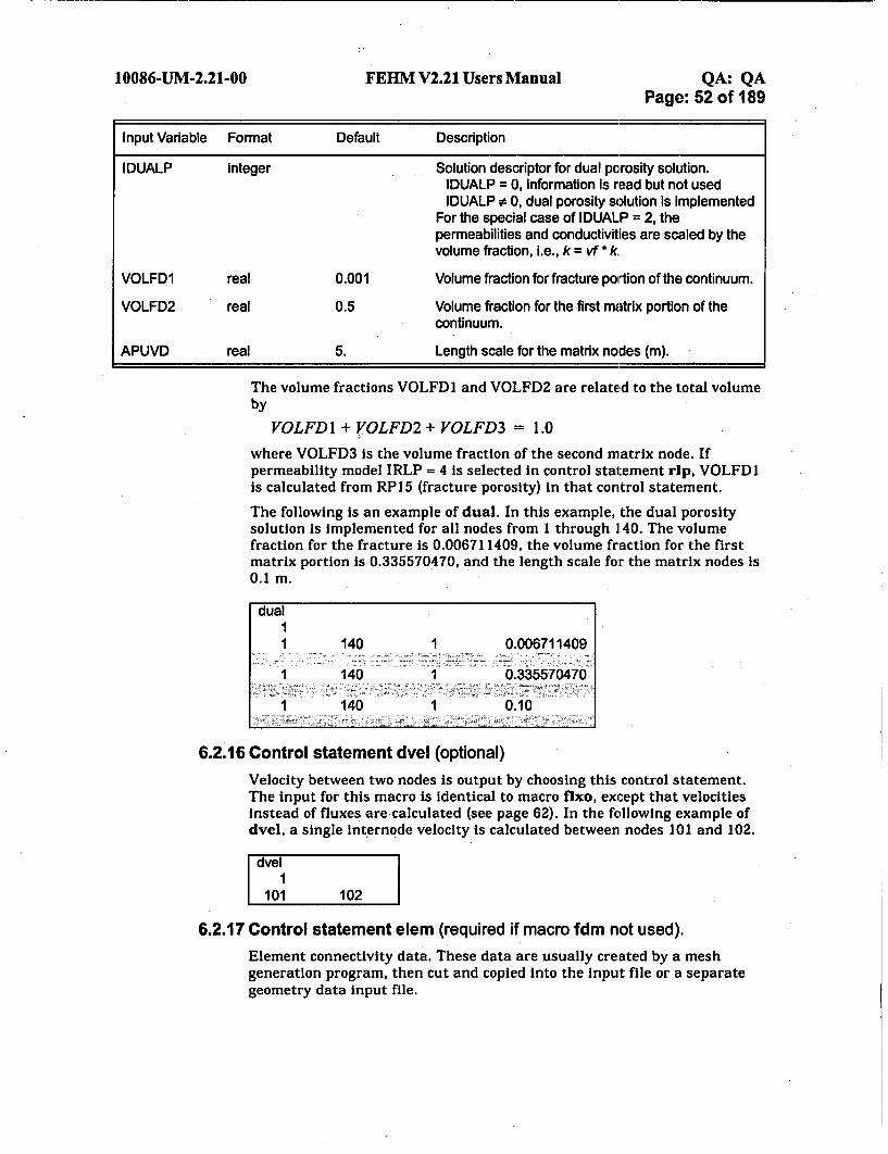
10086-UM-2.21-OO FERM V2.21 Users Manual QA: QAPage: 52 of 189
Input Variable Format Default Description
IDUALP integer Solution descriptor for dual porosity solution.IDUALP = 0, information is read but not usedIDUALP •0, dual porosity solution is Implemented
For the special case of IDUALP = 2, thepermeabilities and conductivities are scaled by thevolume fraction, i.e., k = vf * k.
VOLFD1 real 0.001 Volume fraction for fracture portion of the continuum.
VOLFD2 real 0.5 Volume fraction for the first matrix portion of thecontinuum.
APUVD real 5. Length scale for the matrix nodes (m).
The volume fractions VOLFD1 and VOLFD2 are related to the total volume
by
VOLFD 1+ VOLFD2 + VOLFD3 = 1.0
where VOLFD3 Is the volume fraction of the second matrix node. Ifpermeability model IRLP = 4 is selected in control statement rip, VOLFD1is calculated from RP15 (fracture porosity) in that control statement.
The following is an example of dual. In this example, the dual porositysolution is implemented for all nodes from 1 through 1.40. The volumefraction for the fracture is 0.006711409, the volume fraction for the firstmatrix portion is 0.335570470, and the length scale for the matrix nodes is0.1 m.
dual11 140 1 0.006711409
1 140 1 0.335570470
1 140 1 0.10
6.2.16 Control statement dvel (optional)
Velocity between two nodes is output by choosing this control statement.The input for this macro is identical to macro flxo, except that velocitiesinstead of fluxes are calculated (see page 62). In the following example ofdvel, a single internode velocity is calculated between nodes 101 and 102.
dvel1
101 102
6.2.17 Control statement elem (required if macro fdm not used).
Element connectivity data. These data are usually created by a meshgeneration program, then cut and copied into the input file or a separategeometry data input file.

10086-UM-2.21-00 FEHM V2.21 Users Manual QA: QAPage: 53 of 189
Group I - NS, NEI
Group 2 - MB, NELM (1), NELM (2),..., NELM (NS)
IF NS < 0 then ABS(NS) is interpreted as the number of nodes perelement. NS < 0 signals the code to make rectangles (or bricks in threedimensions) a sum, of triangles (or tetrahedrals). This provides morestability in nonlinear problems with a distorted mesh. Figure 2 showsavailable element types and the nodal numbering convention. To end thecontrol section a blank line is entered.
Input Variable Format Description
NS integer Number of nodes per element.
NEI integer Number of elements
MB integer Element number.-If MB < 0 then the difference between the absolutevalue of MB and the previous absolute value of MB is used togenerate intermediate values by interpolation in the code.
NELM (1) integer First node of element MB
NELM (2) integer Second node of element MB
NELM (NS) integer Last node of element MB
The following is an example of elem. In this example there are 4 nodes perelement, i.e., thp elements are 2-dimensional quadrilaterals,. There are atotal of 117 elements in the model, element number 1 Is defined by nodes15, 16, 2, and 1, element number 2 is defined by nodes 16, 17, 3 and2, andso on.
elem4 1171 15 16 2 12 16 17 3 2
10 24 25 11 1011 25 26 12 1112 26 27 13 12
116 138 139 125 124117 139 140 126 125
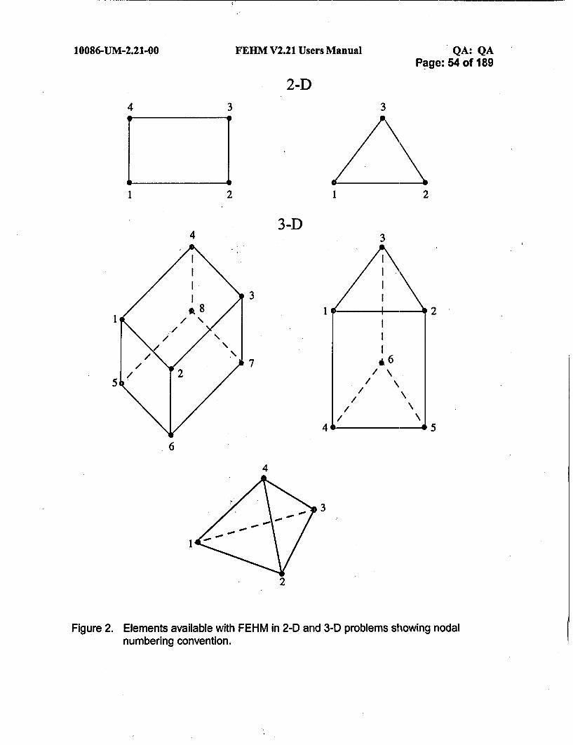
10086-UM-2.21-0O FEHM V2.21 Users Manual QA: QAPage: 54 of 189
2-D4 3 3
1 2I 2
3-D4 3
31 2
7
4 5
6
4
3
11
Figure 2. Elements available with FEHM in 2-D and 3-D problems showing nodalnumbering convention.

10086-UM-2.21-00 FEHM V2.21 Users Manual QA: QAPage: 55 of 189
6.2.18 Control statement eos (optional)
Equation of State. Provide the code with alternate thermodynamicproperties for the liquid and/or vapor phases. (This is one way in which thecode may be instructed to simulate nonisothermal, single phase air. It mayalso be used to make comparisons between the code and analyticalsolutions that use different equations of state.)
Group 1 - IIEOSD, IPSAT, ITSAT
Group 2 - EWI, EW2, EW3, EW4, EW5, EW6, EW7, EW8, EW9, EW10,EW11
Group 3- EVI, EV2, EV3, EV4, EV5, EV6, EV7, EVS, EV9, EV1O, EVIl
For calculation of the simplified thermodynamic equations the above datais used to generate first order equations. The exception to this is theviscosity of the liquid and use of the ideal gas law. The viscosity of theliquid uses a 1/T term. For the calculation of vapor density and itsderivatives, the ideal gas law is used instead of a linear relationship. Thus,EV4 and EV5 are not used, but are included so the format is the same asthat for the liquid parameters in Group 2.
Input Variable Format Description
IIEOSD integer Equation of state reference number. When IIEOSD = 1 or 2 are used,they refer to the high and low pressure data sets, respectively, in FEHM.For these values the input-in Group 2 and Group 3 will be ignored afterit is entered. When any value other than 1 or 2 are used, the user-defined equation of state is used with Groups 2 and 3 for input.
IPSAT integer Parameter to set vapor pressure to zero. If IPSAT # 0 the vaporpressure is set to zero, otherwise the vapor pressure is calculated in thecode.
ITSAT integer Parameter to adjust the saturation temperature. If ITSAT < 0, thesaturation temperature is set to -10000C. If ITSAT > 0, the saturationtemperature is set to 1000CC. If ITSAT = 0, the calculated value is used.
EWI real Liquid reference pressure (MPa).
EW2 real Liquid referenbe temperature (°C).
EW3 real Liquid reference density (kg/m 3).
EW4 real Derivative of liquid density with respect to pressure at referenceconditions.
EW5 real Derivative of liquid density with respect to temperature at reference
conditions.
EW6 real Liquid reference enthalpy (MJ/kg).
EW7 real Derivative of liquid enthalpy with respect to ptessure at referenceconditions.
EW8 real Derivative of liquid enthalpy with respect to temperature at referenceconditions.

10086-UM-2.21-OO FEHM V2.21 Users Manual QA: QAPage: 56 of 189
Input Variable Format Description
EW9 real Liquid reference viscosity (Pa s).
EW10 real Derivative of liquid viscosity with respect to pressure at referenceconditions.
EW1 1 real Derivative of liquid viscosity with respect to temperature at referenceconditions.
EV1 real Vapor reference pressure (MPa).
EV2 real Vapor reference temperature (0C).
EV3 real Vapor reference density (kg/m 3 ).
EV4 real Not used, included only to maintain a similar format to Group 2. Densityvariation with pressure governed by ideal gas law.
EV5 real Not used, included only to maintain a similar format to Group 2. Densityvariation with temperature governed by ideal gas law.
EV6 real Vapor reference enthalpy (MJ/kg).
EV7 real Derivative of vapor enthalpy with respect to pressure at referenceconditions.
EV8 real Derivative of vapor enthalpy with respect to temperature at referenceconditions.
EV9 real Vapor reference viscosity (Pa s).
EV1 0 real Derivative of vapor viscosity with respect to pressure at referenceconditions.
EVI1 real Derivative of vapor viscosity with respect to temperature at referenceconditions.
The following Isan example of eos. In this example, a user-definedequation of state is specified and the vapor pressure and saturationtemperature are calculated in the code. For liquid properties, the referencepressure is 0.1 MPa, the reference temperature is 20 °C, and the referencedensity is 998. kg/m 3, the derivative of density with respect to pressure iszero and with respect to temperature is -0.2 kg/m3/°C. The referenceenthalpy is 0.88 MJ/kg, the derivative of enthalpy with pressure is zero,and the derivative with temperature is 4.2e-03 MJ/kg/°C. The referenceviscosity is 9.e-04 Pa-s and the derivatives of viscosity with pressure andtemperature are zero. For vapor properties, the reference pressure is 0.1MPa, the reference temperature is 20 °C, and the reference density is 1.29kg/m 3 . The reference enthalpy is 2.5 MJ/kg, the derivative of enthalpy withpressure is 0, and with temperature is 0.1 MJ/kg/°C. The referenceviscosity is 2.e-4 Pa-s and its derivatives with pressure and temperatureare zero.

10086-UM-2.21-00 FEHM V2.21 Users Manual QA: QAPage: 57 of 189
eos3 0 0
0.1 20. 998 0. -0.2 0.88 0. 4.2e-3 9.e-4 0. 0.0.1 20. 1.29 0. 0. 2.5 0. 0.1 2.e-4 0. 0.
6.2.19 Control statement exrl (optional)
Allows the user to choose linearized relative permeability. The linearizedrelative permeability is formed using the nonlinear value of relativepermeability at the iteration number IEXRLP. After that iteration arelative permeability value based on a Taylor series expansion insaturation is used.
Group 1 - IEXRLP
In the following example of exrl, the user enables linearized relativepermeability at -the first iteration.
6.2.20 Control statement fdm (required if macro coor and elem not used)
Finite difference input.
Group 1 - KEYWORD
Group 2 - MODCHAR (only if KEYWORD is "modf")
or
Group 2 - NX, NY, NZ (if KEYWORD is "block" or "poin")
Group 3 - XO, YO, NO (only if KEYWORD is 'block)
Group 4 - MB, COORDINATE (X, Y or Z) (if KEYWORD Is 'poln")
or
Group 4 - MB, SPACING (DX, DY, DZ) (if KEYWORD is "bloc")
Group 4 is repeated for each NX, NY, and NZ, i.e., all X data are input,followed by Y data, followed by Z data for each division terminated by ablank line.

10086-UM-2.21-OO FEHM V2.21 Users Manual QA: QAPage: 58 of 189
Input Variable Format Description
KEYWORD character*4 Keyword indicating format of finite difference input to follow ("block","poin", or "modf").
MODCHAR character*132 If the keyword is "modf", the name of a modflow geometry data file isinput and the finite difference input is read from that file and no otherdata is input.
NX integer Number of divisions in the x direction.
NY integer Number of divisions in the y direction.
NZ integer Number of divisions in the z direction.
X0 real Coordinate of x origin point (m).
YO real Coordinate of y origin point (m).
ZO real Coordinate of z origin point (m).
X real X coordinate (m).
Y real Y coordinate (m).
Z real Z coordinate (m).
DX real Node spacing in the x direction (m).
DY real Node spacing in the y direction (m).
DZ real Node spacing in the z direction (m).
MB integer Division number. If the division number is negative the code willspace each divison from the previous to the current proportionalto the assigned spacings.
In the following example of fdm, the "block" format is used.There isIdivision in the X and Y directions, and 50 divisions in the Z direction. Thespacing is 1 m in the X and Y directions, and 0.002 m for each division inthe Z direction.
fdmblock
1 1 500. 0. 0.1 1.0
1 1.0
1 0.002-50 0.002
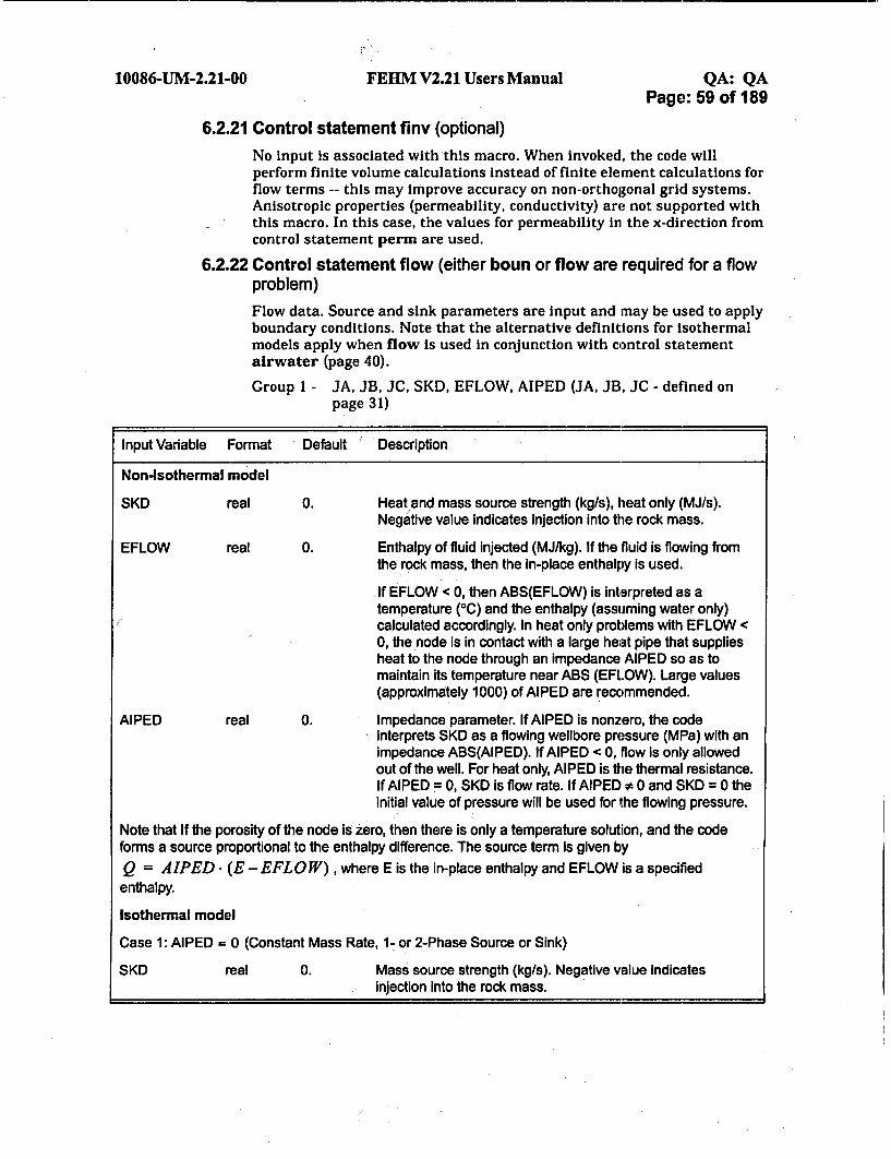
10086-UM-2.21-00 FEHM V2.21 Users Manual QA: QAPage: 59 of 189
6.2.21 Control statement finv (optional)
No input is associated with this macro. When invoked, the code willperform finite volume calculations instead of finite element calculations forflow terms -- this may improve accuracy on non-orthogonal grid systems.Anisotropic properties (permeability, conductivity) are not supported withthis macro. In this case, the values for permeability in the x-direction fromcontrol statement perm are used.
6.2.22 Control statement flow (either boun or flow are required for a flowproblem)Flow data. Source and sink parameters are input and may be used to applyboundary conditions. Note that the alternative definitions for isothermalmodels apply when flow is used in conjunction with control statementairwater (page 40).
Group 1 - JA, JB, JC, SKD, EFLOW, AIPED (JA, JB, JC - defined onpage 31)
Input Variable Format Default Description
Non-Isothermal model
SKD real 0. Heat and mass source strength (kg/s), heat only (MJ/s).Negative value indicates injection into the rock mass.
EFLOW real 0. Enthalpy of fluid injected (MJ/kg). If the fluid is flowing fromthe rock mass, then the in-place enthalpy is used.
If EFLOW < 0, then ABS(EFLOW) is interpreted as atemperature (°C) and the enthalpy (assuming water only)calculated accordingly. In heat only problems with EFLOW <0, the node is in contact with a large heat pipe that suppliesheat to the node through an impedance AIPED so as tomaintain its temperature near ABS (EFLOW). Large values(approximately 1000) of AIPED are recommended.
AIPED real 0. Impedance parameter. If AIPED is nonzero, the codeinterprets SKD as a flowing wellbore pressure (MPa) with animpedance ABS(AIPED). If AIPED < 0, flow is only allowedout of the well. For heat only, AIPED is the thermal resistance.If AIPED = 0, SKD is flow rate. If AIPED # 0 and SKD = 0 theinitial value of pressure will be used for the flowing pressure.
Note that If the porosity of the node iS zero, then there is only a temperature solution, and the codeforms a source proportional to the enthalpy difference. The source term is given by
Q = AIPED* (E - EFLOW) , where E is the in-place enthalpy and EFLOW is a specifiedenthalpy.
Isothermal model
Case 1: AIPED = 0 (Constant Mass Rate, 1- or.2-Phase Source or Sink)
SKD real 0. Mass source strength (kg/s). Negative value indicatesinjection into the rock mass.

10086-UM-2.21-OO FEHM V2.21 Users Manual QA: QAPage: 60 of 189
Input Variable Format Default Description
EFLOW real 0.
AIPED real 0.
Case 2: AIPED > 0 (Constant Pressure,
SKD real 0.
EFLOW real 0.
a) EFLOW > 0, EFLOW is the source liquid saturation,
= SKD. EFLOW (kg/s),
Qa SKD. (I -EFLOW) (kgts)
b) EFLOW < 0, ABS(EFLOW) is the source air pressure(MPa)
Q = SKD (kg/s)
Qa = 1.0 -(Pa -ABS(EFLOW)) (kg/s)
In the above and following relations, Qw, is the source term
for water, Qa is the source term for air, and Pa is the in-place
air pressure. The second case works well in situations whereinflow is specified and it is desired to hold the air pressure at aconstant value.
Used only as flag to indicate Constant Mass Rate.
Constant Liquid Saturation Source or Sink)
Specified source air pressure (MPa).
a) EFLOW < 0, air only source.
Qa = AIPED. (Pa - SKD) (kg/s)
b) 0 < EFLOW < 1, EFLOW is specified source liquidsaturation, for SKD > 0, 2-phase source,
Qa = AIPED. (Pa - SKD) (kg/s)
Qw = AIPED. (SI-EFLOW) (kg/s)
when SKD < 0, water only source Qa = 0.
In the above relation S, is the in-place liquid saturation.
Impedance parameter. A large value is recommended(102 - 106) in order to create a flow term large enough tomaintain constant pressure.
AIPED real
Case 3: AIPED < 0 (Outflow only, if P1 > SKD)
SKD
EFLOW
AIPED
real
real
real
0.
0.
0.
Pressure above which outflow occurs (MPa)
Not used.
Impedance parameter.
Q = ABS(AIPED) . R1/.tl(P 1 - SKD) (kg/s)
where R, Is the water relative permeability and g, is the
water viscosity.

10086-UM-2.21-OO FEHM V2.21 Users Manual QA: QAPage: 61 of 189
The following are examples of flow. In the first example, at node 88, amass flux of 0.05 kg/s at 25 0C is being withdrawn from the model. Becausefluid is being withdrawn the in-place temperature will actually be used.For every 14th node from node 14 to 140, the pressure and temperature arebeing held constant at 3.6 MPa and 160 0C, respectively. This represents aconstant temperature recharge along one of the problem boundaries.
flowI
88 88 1 0.050 -25.0 0.14 140 14 3.600 -160.0 1.
In the second example, the corresponding input for alirwater (page 40), isincluded, indicating an isothermal air-water two-phase simulation is beingrun with a reference temperature for property evaluation of 20 *C and areference pressure of 0.1 MPa. At nodes 26 and 52, water saturation is100% and water is being injected at 2.e-3 kg/s. At nodes 1 and 27, there isan air only source, with a specified pressure of 0.1 MPa, and the air isbeing injected at the rate of 100*(Pa - 0. 1) kg/s.
airwater2
20.0 0.1flow
26 52 26 -2.e-3 1.0 0.1 27 26 0.1 -0.2 1.e2
6.2.23 Control statement flo2 (optional)
Group 1 - JA, JB, JC, JD, SKD, EFLOW, AIPED (SKD, EFLOW, AIPED -defined on page 59 under control statement flow)
Multiple lines of input may be used, terminated by a blank line.
Input Variable Format Description
JA integer Indices used to define planes in a 3-D simulation with a regularnumbering pattern. The flow rates are defined within the inner loop of
JB integer the do loops:
JC integer DO JK = JA, JBKL = JK - JADO IJ = JA + KL, JC + KL, JD
JD integer ...ENDDO
ENDDO
6.2.24 Control statement flo3 (optional)
Alternate format for flow data for a seepage face.
Group I - JA, JB, JC, PFLOW, ESK, AIPED, KA (JA, JB, JC - defined onpage 31)

10086-UM-2.21-OO FEHM V2.21 Users Manual QA: QAPage: 62 of 189
Input Variable Format Description
PFLOW real Ambient pressure (MPa) or flow area (mi2 )
ESK real Not used
AIPED real Same as above for AIPED under keyword "flow"
KA integer Flag to indicate seepage face (-3) or unit gradient flux (-2)
6.2.25 Control statement floa (optional)The input for this macro is identical to macro flow, except that it isrelevant only to fluxes and the values are additive to existing fluxes for thedefined nodes.
6.2.26 Control statement fixo (optional)
Mass flux between two nodes is output by choosing this control statement.
Group 1 - NFLX
Group 2 - IFLXI, IFLX2 (repeated NFLX times)
Group 3 - XI, Y1, ZI (as needed)
Group 4- X2, Y2, Z2 (as needed)
If IFLX1 < 0, then after all IFLX1 and IFLX2 values are read, coordinatesXl, Yl, and Z1 are read and the node nearest to these coordinates is used.If IFLX2 < 0, coordinates for the second node are read in on another line.The code cycles through each IFLX1 and IFLX2 in this manner, readingcoordinates when needed. Results are written to the screen if tty output isenabled and to the output file iout.
Input Variable Format Description
NFLX integer Number of internode fluxes to be calculated.
IFLX1 integer First node to be used in flux calculation.
IFLX2 integer Second node to be used in flux calculation. If IFLX2 = 0, then thenode connected to IFLX1 with the greatest internodal distance isused to calculate the mass flux.
X1 real Coordinates of the first node to be used in flux calculation. Used onlyfor those nodes where IFLX1 < 0.
Y1 real
ZI real
X2 real Coordinates of the second node to be used in flux calculation. UsedY2 real only for those nodes where IFLX2 <i 0.
Z2 real :1
The following are examples of flxo. In these examples, one internode flux Iscalculated.In the first case (left), from the node numbered 193 to the node

10086-UM-2.21-00 FEIIM V2.21 Users Manual QA: QAPage: 63 of 189
numbered 195, and in the second case (right) between nodes closest tocoordinates 0., 0., 0. m and 20., 20., 20. m.
fixo
193 195
fixo
-1 -70. 0. 0.
20. 20. 20.
6.2.27 Control statement flxz (optional)
Total water flux through a zone is output by choosing this controlstatement. When this macro is invoked, the following output is given atevery heat and mass transfer time step:
• The sum of all fluid source flow rates for each zone
* The sum of all fluid sink flow rates for each zone
* The net flux passing through each zone
" The net source/sink flux for each zone
Zones must be defined using macro zone prior to using this macro.
Group 1 - NFLXZ
Group 2 - IFLXZ(I), I = 1, NFLXZ
Input Variable Format Description
NFLXZ integer Number of zones for which output for water flux through the zone isw~itten.
IFLXZ integer Zone numbers for which water flux output is written (NFLXZ zones)
The following is an example of flxz. In this example water flux throughzones 1, 6 and 10 will be output.
flxz31 6 10
6.2.28 Control statement fper (optional)
Assign permeability scaling factors.
Group 1 - JA, JB, JC, SCALEX, SCALEY, SCALEZ (JA, JB, JC - definedon page 31)
Input Variable Format Default Description
SCALEX real 1.0 Permeability scaling factor in the x-direction.
SCALEY real 1.0 Permeability scaling factor in the y-direction.
SCALEZ real 1.0 Permeability scaling factor in the z-direction.

10086-UM-2.21-00 FEHM V2.21 Users Manual QA: QAPage: 64 of 189
The following is an example of fper. In this example, the values of thepermeability (defined in a previous perm macro) are multiplied by 1.0 inthe X direction, 0.5 in the Y direction, and 0.1 in the Z direction.
1 r 140 1 1.0 0.5 0.1
6.2.29 Control statement frip (optional)
Relative permeability factors for residual air effect.
Group I - JA, JB, JC, RLP_FAC (liquid), RLPFAC (vapor) (JA, JB, JC -defined on page 31)
Input Variable Format Description
RLPFAC (liquid) real Residual liquid relative permeability value (i =1 to nO).
RLPFAC (vapor) real Residual vapor relative permeability value (i = nO + 1 to 2*nO).
6.2.30 Control statement gdpm (optional)
Data to define the parameters in the Generalized Dual Porosity modelformulation.
Group 1 - GDPM_FLAG, NGDPMNODES
Group 2- NGDPMLAYERS(I), VFRAC_PRIMARY(I), (GDPMX(IJ),J=I,NGDPMLAYERS(I))- an arbitrary numbers of lines ofinput, terminated by a blank line.
Group 3 - JA, JB, JC, IGDPM (JA, JB, JC - defined con page 27)
Input Variable Format Description
GDPMFLAG integer Flag to denote that the GDPM model option is being invoked. Thedefault is 0 if GDPM is not being used. If 1, matrix node geometry isparallel fractures; if 2, matrix node geometry is spherical, with thefractured medium residing at the exterior of an idealized sphericalblock, and transport occurs into the block,
NGDPMNODES integer Total number of matrix nodes present in the simulation. Since thisnumber may not be known at runtime, the cod,6emay be run oncewith a placeholder value for NGDPMNODES. If the number isincorrect, the code will report the appropriate value and stop. Thisvalue can then be entered and the simulation will proceed when thecode is rerun.
NGDPMLAYERS integer The number of matrix nodes specified for this model number. Allprimary nodes assigned to this model number, (using the IGDPMinput below) will have NGDPMLAYERS matrix nodes.
VFRACPRIMARY real The fraction of the total control volume that is assigned to theprimary porosity. Then, 1-VFRAC_PRIMARY is the fraction ofthe control volume that is divided among the dual porositynodes.

10086-UM-2.21-OO FEHM V2.21 Users Manual QA: QAPage: 65 of 189
Input Variable Format Description.
GDPMX real The matrix discretization distances for the matrix nodes associatedwith this model (units of meters). Grid points are placed at thesevalues to discretize each matrix block. There must beNGDPMLAYERS values, entered in ascending order. Forthe parallel plate geometry, the final value is the distance tothe centerline between the fractures, and for the sphericalgeometry, the final value is the radius of the sphere.
IGDPM integer Model number for parameters defined in group 2. These values areassigned only for the primary nodes. The default is 0, which denotesthat there are no dual porosity nodes at that primary node.
Based on the input in this macro, the code internally assigns nodenumbers, finite element coefficients, and reconstructs the connectivityarray for the grid' The original nodes in the grid (the primary nodes) retainthe node numbers 1 to NEQ_PRIMARY, where NEQ_1RIMARY is thenumber of nodes assigned in the macro coor. The matrix nodes areassigned numbers from NEQPRIMARY + 1 to NEQPRIMARY +NGDPMNODES. To assign matrix node numbers, the code loops througheach primary node, and if GDPM nodes are specified, assigns the nodenumbers in increasing order within the matrix block of that primary node.[Note that the user is responsible for assigning rock, hydrologic, andtransport properties for the matrix nodes as well as the primary nodes. Forinput using zones, this process is facilitated with the convention that zonenumbers associated with matrix nodes are set to ZONE_.DPADD + the zonenumber for the corresponding fracture node (see page 31). This conventionis overwritten for any matrix node for which the user assigns a zonenumber using the 'nnum' option in the macro zone.]
For output, the code can report time-varying values in the ".out", .. his",and ".trc" files for both primary and matrix nodes, but fields written for theentire grid (for example, in the AVS output using the macro cont) areoutput only for the primary nodes.
The following is an example of gdpm. In this example the matrix nodegeometry is parallel to the fractures and there are 1479 matrix nodesdistributed in 29 layers. A single model is defined which is applied to theentire problem Qrmain.
gdpm1 1479
29 .0001 .001 .002 .003 .004 .006 .009.019 .02901 .03901 .04901 .05901 .09902 .19904 .29906.39908 .49910 .59912 .69914 .79916 .89918 .99920 1.49931.9994 2.4995 2.9996 3.4997 3.9998 4.4999 5.0000
1 0 0 1
6.2.31 Control statement grad (optional)
Gradient model input.
Group 1 - NGRAD

10086-UM-2.21-OO FEHM V2.21 Users Manual QA: QAPage: 66 of 189
Group 2 - IZONEGRAD, CORDG, IDIRG, IGRADF, VARO, GRAD1
Input Variable Format Description
NGRAD integer Number of gradient models.
IZONEGRAD integer Zone associated with ith model
CORDG real Fiducial point of gradient equation.
IDIRG integer Coordinate direction of gradient.
IGRADF integer Variable to which gradient is applied.IGRADF = 1, PressureIGRADF = 2, TemperatureIGRADF = 3, Saturation
VARO real Value of variable at fiducial point.
GRAD1 real Gradient with distance.
The following is an example of grad. A temperature gradient in the Ydirection from the fiducial point of 0 will be applied to zone 1.
grad
11 0'. 2 210. -10
6.2.32 Control statement head (optional)
Hydraulic head values are used for input and output instead of pressures.Use of this macro enables the Boussinesq approximation (bous macro) andisothermal air-water two-phase simulation (airwater macro)automatically. It affects the pres and flow macros by requiring headinformation where pressure values were previously required. The default isto have no input associated with this macro. However, an optional headincrement can be given after the head macro keyword. This value will beadded to all input head values to ensure a single phase fluid state.
The following is an example of head. In this example the optional headincrement is included and a value of 1000. m is added to all input headvalues.
head 1000.

10086-UM-2.21-00 FEHM V2.21 Users Manual QA: QAPage: 67 of 189
6.2.33 Control statement hflx (optional)
Heat flux input.
Group 1 - JA, JB, JC, QFLUX, QFLXM (JA, JB, JC - defined on page 31)
A negative heat flux indicates heat flow into the reservoir.
Input Variable Format Default Description
QFLUX real 0. If QFLXM = 0, then QFLUX is the heat flux (MW). IfQFLXM * 0, then QFLUX Is a temperature (°C) andthe heat flux is calculated according to the formula:
QH = QFLXM * (T - QFL UX) (MW).
QFLXM real 0. If QFLXM > 0, multiplier for heat flux equation givenin QFLUX description (MWI°C). This must be largefor large temperature gradients, or when a constanttemperature must be maintained.If QFLXM < 0, then QFLUX is interpreted as a fixedsaturation and
QH = ABS(QFLXM) 9 (St- QFLUX) (MW)
The following is an example of hflx. In this example, at each node from 401to 410, a heat flux of 0.001 MW is being injected into the model.
Ihflx
401 410 1 -0.001 0.0
6.2.34 Control statement hyco (required if macro perm not usedl)
Hydraulic conductivity input.
Group 1 - JA, JB, JC, PNXD, PNYD, PNZD (JA, JB, JC - defined onpage 31)
Input Variable Format Default Description
PNX real 1.e-30 Hydraulic conductivity in the x-.direction (m/s).
PNY real 1 .e-30 Hydraulic conductivity in the y-direction (m/s).
PNZ real 1 .e-30 Hydraulic conductivity In the z-direction (m/s).
The following is an example of the hyco macro. In this example, nodes 1through 140 are specified to have hydraulic conductivities in the X, Y, andZ directions of 1.Oe-5, 1.0e-5, and 0. m/s respectively.
hyco1 140 1 1 .00e-05 1 .00e-05 0.00e-00

10086-UM-2.21-00 FEHM V2.21 Users Manual QA: QAPage: 68 of 189
6.2.35 Control statement Ice or meth (optional)
Ice phase calculations, not tested.
Group 1 - ICE, SIIN, TMELT
Group 2 - JA, JB, JC, SII (JA, JB, JC - defined on page 31)
Input Variable Format Description
ICE integer Solution descriptor for ice solution.ICE = 0, information is read but not used.ICE •0, Ice solution is implemented.
SIIN real Default value for ice saturation (used when ice saturation SII inGroup 2 is set to 0 at any node).
TMELT - real Freezing temperature of water (°C).
SiI real Ice saturation. The default value is [0].
6.2.36 Control statement impf (optional)
Time step control based on maximum allowed variable change.
Group 1 - DELPT, DELTT, DELST, DELAT
Input Variable Format Description
DELPT real Maximum allowable pressure change for which time step will beincreased. (MPa)
DELTT real Maximum allowable temperature change for which time step will beincreased. (°C)
DELST real Maximum allowable saturation change for which time step will beincreased.
DELAT real Maximum allowable air pressure change for which time step will beincreased. (MPa)
The following is an examples of impf. In this example, pressure changesare limited to 0.5 MPa, temperature changes to 20 *C, saturation changesto 0.1, and air pressure changes to 0.05 MPa during a time step.
impf 20.0 0.1 0.05]
6.2.37 Control statement Init (required if macro pres not used)
Set initial pressure and temperature at all nodes.
Group 1 - PEIN,,TIN, TINI, GRADI, DEPTH, TIN2, GRAD2, QUAD
Note that the macro pres may overwrite some of the values that are set bymacro init.

10086-UM-2.21-0O FEHM V2.21 Users Manual QA: QAPage: 69 of 189
Input Variable Format Description
PEIN real Initial value of pressure (MPa). If initial values are read from the readfile (iread), then this value Is ignored. If gravity is present, this is thevalue of the pressure at node 1, and the other nodal pressures areadjusted by applying the hydraulic head. Absolute pressures areused. Pressure as a function of depth is calculated with TIN < 0.
TIN real Initial value of temperature (°C). If TIN < 0, then the initialtemperatures are calculated using the temperature gradient formulasgiven below.
TIN1 real Defined in formulas below (°C)
GRAD1 real Defined in formulas below (°C/m)
DEPTH real Defined in formulas below (m)
TIN2 real Defined in formulas below (°C)
GRAD2 real Defined in formulas below (°C/m)
QUAD real Defined in formulas below (°C/m 2)
T = TIN1 + GRAD1 xZ, 0<Z<DEPTH
2T = TIN2 + GRAD2 x Z + QUAD x Z, Z > DEPTH
The following are examples of Init. In the first example, the Initialpressure Is 3.6 MPa and the initial temperature Is 240 'C over the entirerange of depth for the model.
7 3;7 0.0 240. .0. 0. 240. 0. 0.
In the second example, the initial pressure Is 5.0 MPa and the initialtemperature field is defined using a surface temperature of 20 TC andlinear gradient of 0.3 0C/m for depths ranging from 0 - 2500 m.
init 5.0 0.0 20. 0.3 2500. 20. 0.3 0.
6.2.38 Control statement isot (optional)
If used, assumes an Isotropic geometry for area coefficients. The isotropicassumption results in a saving of up to 1/3 for coefficient storage. No inputis associated with this macro.
6.2.39 Control statement Iter (optional)
If the user Is not familiar with the linear equation solver routines in FEHM(Zyvoloski and Robinson, 1995) control statement Iter should not be used.
Group I - GI, G2, G3, TMCH, OVERF
Group 2 - IRDOF, ISLORD, IBACK, ICOUPL, RNMAX
~v.

10086-UM-2.21-00 FEHM V2.21 Users Manual QA: QAPage: 70 of 189
The parameters Gl, G2, and G3 are used to calculate the completioncriteria for the linear equation solver. The equation for the stoppingcriteria is:
EPE = G3*max(TMCH, max(FO, min(GI*SQRT(R**2), G2*R**2)))
where R**2 is the sum-squared of the equation residuals, and FO is the
SQRT(RO**2)*EPM for the first iteration (see macro ctrl for a definitionof EPM). The other parameters are defined below.
Input Variable Format Default Description
G1 real 1 .e-6 Multiplier for the linear convergence region of theNewton-Raphson iteration.
G2 real 1 .e-6 Multiplier for the quadratic convergence region of theNewton-Raphson iteration.
G3 real 1 .e-3 Multiplier relating Newton Raphson residuals tostopping criteria for linear solver
TMCH real 1 .e-9 Machine tolerance. If satisfied by the residual norm, theNewton iteration is assumed to be complete. IfTMCH < 0 then the ABS(TMCH) is used as a tolerancefor each equation at each node. Convergence isachieved if the residual of every equation at every nodeis < ABS(TMCH).
OVERF real 1.1 Over relaxation factor for passive nodes in adaptiveimplicit method.
IRDOF integer 0 Enables the reduced degree of freedom method. IfIRDOF = 0, reduced degrees of freedom are notrequired. When IRDOF = 1, a reduced degree offreedom from 3 to 2 or 3 to I is used. When IRDOF = 2,a reduced degree of freedom from 3 to 2 is used. IfIRDOF =11, then an air only solution is found for theisothermal air-water process model. If IRDOF = -11,then the residual for the air equation with the airwatermacro is ignored. If IRDOF =13, then a liquid onlysolution for the airwater macro is assumed.
Examples of 1, 2, 3, 4 and 6 degrees of freedom modelsare:
1 - heat only or mass only.2 - heat and mass, or air-water (isothermal)3 - air-water with heat (non-isothermal)4 - heat and mass, double permeability or air-water
(isothermal), double permeability6 - air-water with heat, double permeability
See Tseng and Zyvoloski (2000) for more informationon the reduced degree of freedom method.
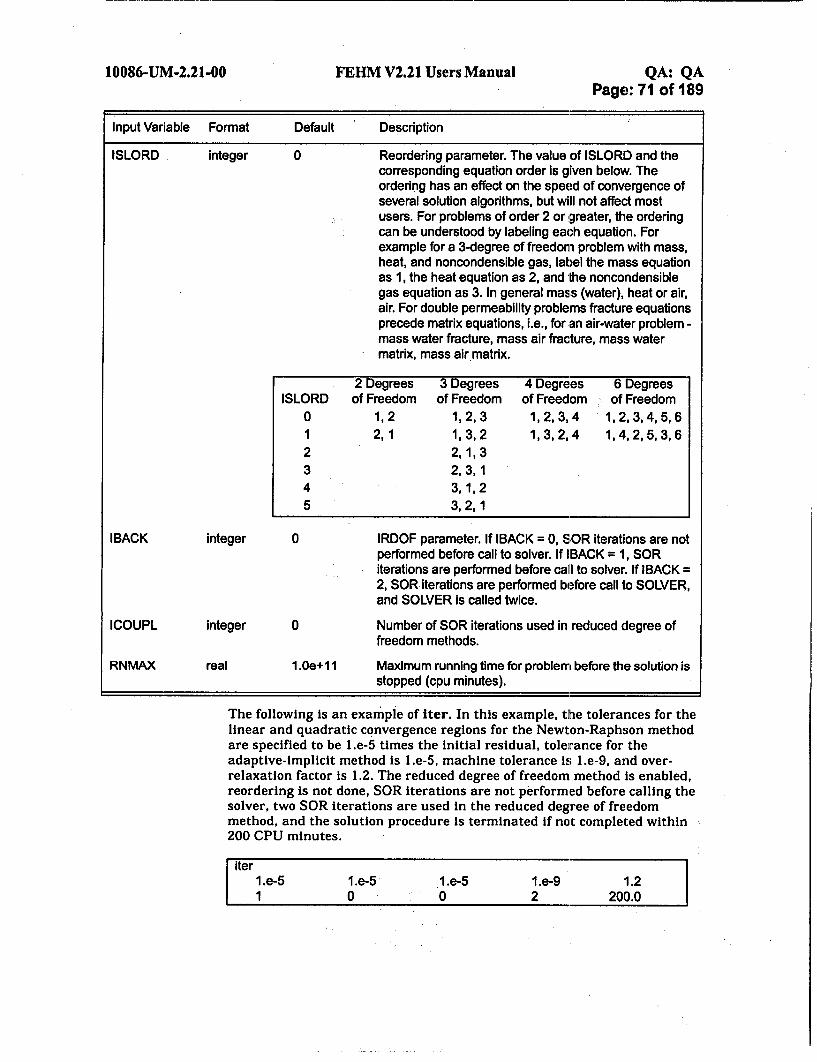
10086-UM-2.21-00 FEHM V2.21 Users Manual QA: QAPage: 71 of 189
Input Variable Format Default Description
ISLORD integer 0 Reordering parameter. The value of ISLORD and thecorresponding equation order is given below. Theordering has an effect on the speed of convergence ofseveral solution algorithms, but will not affect mostusers. For problems of order 2 or greater, the orderingcan be understood by labeling each equation. Forexample for a 3-degree of freedom problem with mass,heat, and noncondensible gas, label the mass equationas 1, the heat equation as 2, and the noncondensiblegas equation as 3. In general mass (water), heat or air,air. For double permeability problems fracture equationsprecede matrix equations, i.e., for an air-water problem -mass water fracture, mass air fracture, mass watermatrix, mass air matrix.
2 Degrees 3 Degrees 4 Degrees 6 DegreesISLORD of Freedom of Freedom of Freedom of Freedom
0 1,2 1,2,3 1,2,3,4 1,2,3,4,5,61 2,1 1,3,2 1,3,2,4 1,4,2,5,3,62 2,1,33 2,3,14 3,1,25 3,2,1
IBACK integer 0 IRDOF parameter. If IBACK = 0, SOR iterations are notperformed before call to solver. If IBACK = 1, SORiterations are performed before call to solver. If IBACK =2, SOR iterations are performed before call to SOLVER,and SOLVER is called twice.
ICOUPL integer 0 Number of SOR iterations used in reduced degree offreedom methods.
RNMAX real 1.0e+1 I Maximum running time for problem before the solution isstopped (cpu minutes).
The following is an example of iter. In this example, the tolerances for thelinear and quadratic convergence regions for the Newton-Raphson methodare specified to be l.e-5 times the initial residual, tolerance for theadaptive-implicit method is 1.e-5, machine tolerance is 1.e-9, and over-relaxation factor is 1.2. The reduced degree of freedom method is enabled,reordering is not done, SOR iterations are not performed before calling thesolver, two SOR iterations are used In the reduced degree of freedommethod, and the solution procedure Is terminated if not completed within200 CPU minutes.
iter I1 .e-5 1 .e-5 1 .e-5 1 .e-9 1.21 0 0 2 200.0

10086-UM-2.21-00 FEHM V2.21 Users Manual QA: QAPage: 72 of 189
6.2.40 Control statement itfc (optional)
Data to define flow and transport parameters at interfaces between pairs ofzones.
Group 1 - ZONEPAIR(I,I),, ZONE-PAIR(I,2), REDFACTOR(I)- an
arbitrary number of lines of input, terminated by a blank line.
Group 2 - (FILTER FLAG(J). J= 1,NSPECI)
Group 3 - ZONECPAIR(K,1), ZONECPAIR(K,2), FTNFACTOR(K)- anarbitrary number of lines of input, terminated by a blank line.
KEYWORD 'file'
SFILENAME
ITFCPORSIZE(I), ITFCPROBSIZE(I)- an arbitrary number oflines of input, terminated by a blank line.
Input Variable Format Description
ZONEPAIR integer Zone number for the zones for which the code identifies theinterface connections when applying the permeability reductionfactor.
REDFACTOR real Reduction factor multiplying the harmonicalHy weighted saturatedpermeability for all connections at the interface identified byZONEPAIR
FILTERFLAG integer FEHM has a provision to apply transport mechanisms for sizeexclusion or filtration at interfaces defined in the itfc macro.These provisions can be used to simulate conditions in which, forexample, abrupt changes in properties occur at interfaces, orhydrologic conditions not explicitly incorporated in a model (a thinclay layer, for example) are thought to be present that affecttransport across the interface. The means for specifying theseinterface transport conditions is the ltfc macro. Thus, thisparameter is a flag used to distinguish whether the size exclusionor filtration is to be implemented (a value 1) or not (a value 0) foreach species Identified in the trac, ptrk, or mptr macros. Thedefault value is 0. See the definition of FTN.FACTOR below fordetails on how to invoke the size exclusion or filtration model.
ZONECPAIR integer Zone number for the zones for which the code identifies theinterface connections when applying the transport filtration or sizeexclusion factors.

10086-UM-2.21-00 FEHM V2.21 Users Manual QA: QAPage: 73 of 189
Input Variable Format Description
FTNFACTOR
KEYWORD
SFILENAME
ITFCPORSIZE
ITFCPROBSIZE
real Filtration or size exclusion factor applied for all connections at theinterface identified by ZONECPAIR. For the trac macro, a sizeexclusion model is implemented, where FTNFACTOR = 0 (sizeexclusion) or1 (no exclusion) are options. For ptrk or mptr, afiltration model is implemented, where the parameter is theprobability of the particle passing through the interface (if 0,filtration is guaranteed; if 1, there is no filtration). For the particletracking model, FTNFACTOR < 0 denotes that the pore sizedistribution is being used. This option is used with the particle sizedistribution option in ptrk and mptr, so that each particle isassigned a size. The cumulative pore size distribution is then usedas a probability distribution function, and when a particleencounters the interface, a pore size is randomly selected fromthe distribution. If the particle is larger than the pore, it is filtered.Note that filtered particles remain at that location in the model andare no longer transported.
character*4 Optional keyword 'file' designating that the pore size distributioninformation is being input in a separate file. This input is enteredonly for interfaces in which FTN_FACTOR < 0 is used.
character*80
real
Optional file name containing the pore size distribution table. Thisinput is entered only for interfaces in which FTNFACTOR < 0 isused.
Pore size for this entry of the pore size distribution table (pairedwith a value of ITFCPROBSIZE). An arbitrary number of entriescpnbe input, terminated with a blank line. These entries arelocated in the file SFILENAME if specified, or in the itfc input fileif the alternate input file is not used. The code decides if particlesare irreversibly filtered by comparing the particle size to therandomly selected pore size. This input is entered only forinterfaces in which FTN_FACTOR < 0 is used.
Cumulative probability for the distribution of pore sizes (pairedwith a value of ITFCPORSIZE). See description of ITFCPORSIZEabove for details. The final entry of the table must haveITFCPROBSIZE = 1, since the distribution is assumed to benormalized to unity. This Input is entered only for interfaces Inwhich FTN_FACTOR < 0 is used.
real
Note that data for each numbered group must be input. The other input isoptional. If filtration is not implemented for any species, a single blank lineis input for Groups 2 and 3, signaling the end of itfc input.
The following is an example of itfc. In this example, the permeabilityreduction factor of 0.1 is applied to all node connections at the interfacebetween zones 6 and 10, or 6 and 11.

10086-UM-2.21-00 FEHM V2.21 Users Manual QA: QAPage: 74 of 189
[i6 10 0.161 0.1
6.2.41 Control statement Itup (optional)
The use of the itup macro is sometimes useful in problems where the flowdirections are changing rapidly. The parameter UPWGT (in macro ctrl)must be greater than 0.5 for this macro to have any effect.
Group I - IAD-UP
Input Variable Format Default Description
lADUP integer 1000 :: Number of iterations after which the upwind directionsare held constant. (A value of 2 is suggested)
In the following example of itup, after 10 iterations the upwind directionsare held constant.
6.2.42 Control statement lupk (optional)
No input is associated with this control statement. This macro enablesupwinding, the technique of evaluating the non-linear equation coefficientsusing the direction of flow relative to the grid block. For example, if flow ismoving from grid blockj to i, the coefficients for block i, are evaluated atthe "upwind" blockj. When upwinding is enabled the full transmissibilityterm will be upwinded (including the intrinsic permeability). Otherwise thefluid and relative permeability part of the transmissibility will beupwinded and the intrinsic permeability will be harmonically averaged.
6.2.43 Control statement mdnode (optional)
Enables extra connections to be made to nodes. This is useful forsimulating wellbore connections, faults, and flow across internalboundaries.
Group 1 - NUMMD, MAXCON, IELIM, SXMULT
Group 2 - NODE, IPAR, NPAR (repeated NUM_MD times)
Input Variable Format Default Description
NUM_MD integer 0 Number of new connections to be entered.
MDMAX integer 0 Maximum number of new connections to a given node. Thisdoes not include old connections. Thus, if a node was alreadyconnected to 5 neighboring nodes and two new connectionswere added to this node in this macro statement and this wasthe maximum number of connections added in this macrostatement, then MDMAX = 2.

10086-UM-2.21-0O FEHM V2.21 Users Manual QA: QAPage: 75 of 189
Input Variable Format Default Description
I_ELIM integer 0 IF IELIM 0, then no action.IF IELIM < 0, then nodal connections are eliminated asneeded if redundant.
SXMULT real*8 1.0 Multiplier for equilibrium conditions.
NODE integer 0 Node to which new connection is established.
IPAR integer 0 IPAR is not used at present. Its value is ignored. However theentered number must be an integer.
NPAR integer 0 NPAR is the new connected node. If NPAR = NODE, no newconnection is established.
The following are examples of mdnode. In the first example (left), 3 newconnections are specified, node 10 is connected to node 15, node 100 isconnected to node 106, and node 10 is connected to node 320. A maximum of2 new connections are allowed per node. The multiplier for equilibriumconditions is set to 10. In the second example (right), 4 new connections arespecified, node 1 is connected to node 16, node 2 is connected to node 1,node 4 is connected to node I and node 10 is connected to node 203. Amaximum of 3 new connections are allowed per node. The multiplier forequilibrium conditions is set to 100.
mdnode3 2 0 10
10 0 15100 0 106
10 0 320
mdnode4 3 0 1001 0 162 0 14 0 1
10 0 203
6.2.44 Control statement mptr (optional)
Multiple species ingrowth particle tracking. Note that data for eachnumbered group must be input. The other input is optional.
Group 1 - NSPECI, MAXLAYERS, MAX-PARTICLES, RIPFEHM
Group 2 - POUT, PRNTRST
Optional keyword "tcurve" is input to indicate that transfer function curvesshould be input to model matrix diffusion. It is followed by NUMPARAMSand TFILENAME.
KEYWORD
NUMPARAMS
TFIItENAME
Optional keyword *zptr" designates zones for breakthrough curves will bedefined. It is followed by IPZONE and IDZONE.
KEYWORD 'zptr'
IPZONE
IDZONE(I) I = 1 to IPZONE

10086-UM-2.21-00 FEHM V2.21 Users Manual QA: QAPage: 76 of 189
Group 3- RSEED
Group 4 - DAYCS, DAYCF, DAYHF, DAYHS
Group 5 is used to define models in which identical transport parametersare assumed to apply. Group 5 data are read until a blank line isencountered. The model number ITRC is incremented by 1 each time a lineis read. Model parameters defined in Group 5 are assigned to nodes orzones using Group6.
KEYWORD 'file'
PFILENAME
For a discussion of optional file use and content see macro ptrk (page 91).The applicable triansport parameters are defined in Group 5 and Group 9.
KEYWORD 'afm'
Group 5 - TCLX(ITRC), TCLY(ITRC), TCLZ(ITRC), APERTUR(ITRC),MATRIXPOR(ITRC)
or when 'afm' is implemented
Group 5 - TCLX(ITRC), TCLY(ITRC), TCLZ(ITRC), APERTUR(ITRC),MATRIXPOR(ITRC), SRESIDUAL(ITRC),GAMMAAFM(ITRC)
Group 6 - JA, JB, JC, ITRC (JA, JB, JC - defined on page 31)
The following groups (Group 7 - 12) are repeated for each species.
Group 7 - ITHSPECI, TRAK_TYPE, HALF.LIFE, IDAUGHTER,CONFACTOR, NEWCONFACTOR, CONFTIME, GMOL,P_FRACTION
KEYWORD 'size'
PARTSIZE(I), PROBSIZE(I) - an arbitrary numbers of lines ofinput, terminated by a blank line.
Note that optional KEYWORD 'size' is only used when colloid transport isenabled.
Group 8 - LAYERS
Group 9 - LAYER_I, TRANSFLAG, KD, RDFRAC, DIFFMFL
or for simulations with colloid (TRANSFLAG < 0)
Group 9 - LAYERI, TRANSFLAG, KD, RDFRAC, DIFFMFL, KCOLL,RCOLL, FCOLL
Group 10 - NS
Group 11- JA, JB, JC, TMPCNSK (JA, JB, JC - defined on page 31)
Note that because the number of source terms is controlled by the valueentered for NS, Group 11 input is not terminated with a blank line.
Group 12 - PINMASS, T1SK, T2SK
For transient source terms, Group 12 is repeated for each time interval andterminated with a blank line. Groups 11 and 12 are repeated for eachsource term (from 1 to NS).

10086-UM-2.21-00 FEHM V2.21 Users Manual QA: QAPage: 77 of 189
For decay-ingrowth calculations, when the particle injection period is toosmall (for example, 1.E-4 days) compared to the half-life of theradionuclides and the half-life is large (for example I.E+9 days), numericalerrors in the decay-ingrowth calculation may arise due to truncation error.To get better accuracy, the user should try to increase the length of theinjection period.
For particle tracking simulations using the transfer function method (seeSection 6.2.3 on page 36 for input file format), it is sometimes desirable toidentify the parameter ranges over which the two- and three-parametertype curves are accessed, so that an assessment can be made regarding thedensity of transfer function curves in a given part of the parameter space.If the flag output~Jlag in the transfer function file is set to "out", the codewrites the real*8 array param-density to the *.out file in the followingformat:
For regular parameter spacings, the output is:
I = 1, numplj = 1, nump2
k = nump3write(lout.*) param..density(i~j,k)
end doend do
end do
For two-parameter models, only the I andJ loops are used. The value ofparam-density is the number of times any particle passes through anynode at those values of the parameters. This allows the user to identifyregions in which a greater density of transfer functions may be required.For the option 'free' in which there is no structure to the parameter gridused for the transfer function curves, nump1 is the total number of curves,and nump2 and nump3 are equal to 1.
Input Variable Format Description
NSPECI integer Number of species in the simulation.
MAXLAYERS integer Maximum number of property layers in the model. The actualnumber of layers used in the model must be !.- MAXLAYERS.
MAXPARTICLES integer Maximum number of particles used for individual species.
RIPFEHM integer Flag to indicate if simulation is coupled with GoldSim.RIPFEHM = 0, FEHM standalone simulationRIPFEHM = 1, GoldSim-FEHM coupling simulation
POUT integer Flag to specify the concentration output format:I - Concentrations computed as number of particles per unit total
volume (rock and fluid)2- Concentrations computed as number of particles per unit fluid
volume (the fluid is liquid for TRAKTYPE = I and gas forTRAKTYPE = 2).
3 - Concentrations computed as number of particles at a givennode point.

10086-UM-2.21-OO FEHM V2.21 Users Manual QA: QAPage: 78 of 189
Input Variable Format Description
PRNT_RST
KEYWORD
integer Flag to specify whether particle information is written to the ".fin"file:
0 - Particle information is not written to "An" file.1 - Particle information is written to the *.fin" file.
character Optional keyword =tcurve" indicating transfer function curve datashould be input to model matrix diffusion. If the keyword is foundthen NUMPARAMS and FILENAME are entered, otherwise they areomitted.
NUMPARAMS
TFILENAME
KEYWORD
IPZONE
IDZONE
RSEED
DAYCS
DAYCF
DAYHF
DAYHS
KEYWORD
PFILENAME
KEYWORD
TCLX
TCLY
TCLZ
integer Number of parameters that define the transfeir function curves beingused.
character Name of input file containing the transfer function curve data.
character*4 Optional keyword 'zptr' designating zones fbr breakthrough curveswill be defined. If no keyword is input, IPZONE and IDZONE arealso omitted.
integer Number of zones for which breakthrough curves are to be output
integer A list of zones for which particle breakthrough data are required.The code outputs the number of particles that leave the system ateach zone IDZONE at the current time step. 'This information iswritten to the ".out" file at each heat and mass transfer time step.
integer 6-digit integer random number seed.
real Time which the particle tracking solution is enabled (days).
real Time which the particle tracking solution is disabled (days).
real Time which the flow solution is disabled (days).
real Tim6 which the flow solution is enabled (days).
character*4 Optional keyword 'file' designating alternate transport parameter fileinput for multiple simulation realizations.
character*80 Name of file from which to read transport parameters.
character*4 Optional keyword 'afm' designating the Active Fracture Model inputfor determining fracture spacing should be used.
real Dispersivity in the x-direction (m). The input value is ignored whendispersion is turned off.
real Dispersivity in the y-direction (m). The input value is ignored whendispersion is turned off.
real Dispersivity in the z-direction (m). The input value is ignored whendispersion is turned off.
APERTUR real Mean fracture aperture (m). The input value is ignored when matrixdiffusion is turned off.

10086-UM-2.21-00 FEHM V2.21 Users Manual QA: QAPage: 79 of 189
Input Variable Format Description
MATRIXPOR
SRESIDUAL
GAMMAAFM
ITRC
ITHSPECI
TRAKTYPE
real
real
real
integer
integer
integer
real
integer
real
HALFLIFE
IDAUGHTER
CONFACTOR
Porosity of the rock matrix. Used to simulate diffusion and sorptionin the rock matrix when matrix diffusion is invoked, otherwise theinput value of MATRIXPOR is ignored.
Residual saturation in the Active Fracture Model used fordetermining the spacing between active fractures. This parameter isonly needed when the keyword 'afm' is included, in which case theinput must be entered. However, the model it; only used in dualpermeability simulations at locations where the finite spacing matrixdiffusion model is invoked.
Exponent in the Active Fracture Model used for determining thespacing between active fractures. See comments for SRESIDUALabove.
Model number for parameters defined in group 5.
Number index of the Ith species.
Flag to denote the fluid phase of the particles:1 - liquid phase particles2 - vapor phase particles
Half-life for irreversible first order decay reaction(s) (days). SetHALFLIFE = 0 for no decay.
Index of the daughter species (i.e., the index number of the speciesto which the current species decays)
If IDAUGHTER = 0, there is no decay and no ingrowth,If IDAUGHTER = -1, there is decay but no ingrowth.
Initial conversion factor for GoldSim-FEHM coupling and FEHMstandalone simulations (# of particles/mole).
For FEHM stand alone simulations: If CONIFACTOR = 0, noconversion is necessary. The input value of PINMASS is thenumber of particles. If CONFACTOR > 0, the code assumes theinput mass is In moles and uses the CONFACTOR to convert itinto number of particles.
For GoldSim-FEHM coupling: If CONFACTOR = 0, at each time'-'tep, the code selects a conversion factor based on the available
memory and the remaining simulation time (end time - currenttime). The code then uses the selected conversion factor tocalculate the number of particles to be injected at the currenttime step. If CONFACTOR > 0, the code uses the product of theCONFACTOR and the input mass (in moles) to calculate theinput number of particles at each time step.
Replace the initial value of CONFACTOR with that specified byNEWCONFACTOR. If NEWCONFACTOR < 0, thenCONFACTOR = -NEWCONFACTOR. If NEWCONFACTOR = 0,use automatic conversion factors,
NEWCONFACTOR real

10086-UM-2.21-00 FERM V2.21 Users Manual QA: QAPage: 80 of 189
Input Variable Format Description
CONFTIME
GMOL
real
real
realP_FRACTION
KEYWORD character*4
PARTSIZE
PROBSIZE
LAYERS
LAYER_I
TRANSFLAG
real
real
integer
integer
integer
The time at which to change the CONFACTOR value to thatspecified by NEWCONFACTOR.
Thei molecular weight of the Ith species. The code uses GMOL andCONFACTOR to convert the mass from number of particles tograms in the final output for GoldSim-FEHM coupling.
The decay-ingrowth particle release factor (percentage of themaximum number of particles released for the parent species).Values are in the range 0. - 1. The default is 0.5.
Optional keyword 'size' designating that the colloid size distributionmodel option is being used (combined with the interface filtrationoption in the itfc macro). If the keyword is not input, PARTSIZEand PROBSIZE are also omitted.
Colloid particle size for this entry of the particle size distributiontable (paired with a value of PROBSIZE). An arbitrary number ofentries can be input, terminated with a blank line. The code assignseach particle a size based on this distribution of particle sizes, anddecides if particles are irreversibly filtered based on the pore sizedistribution assigned in the itfc macro.
Colloid cumulative probability for the distribution of sizes (pairedwith a value of PARTSIZE). See description of PARTSIZE abovefor details. The final entry of the table must have PROBSIZE = 1,since the distribution is assumed to be normalized to unity.
NUmber of layers in which the transport properties of the ith speciesare to be modified. If no property is altered, then set layers=0.
The index number of the ith layer defined in group 5
Flag to specify which transport mechanisms apply[abs(TRANSFLAG)]:
1 - advection only (no dispersion or matrix diffusion)2 - advection and dispersion (no matrix diffusion)
3- advection and matrix diffusion, infinite fracture spacing solution(no dispersion)
4 - advection, dispersion, and matrix diffusion, infinite fracturespacing solution
5 - advection and matrix diffusion, finite fracture spacing solution(no dispersion)
6- advection, dispersion, and matrix diffusion, finite fracturespacing solution
8 - use the the transfer function approach with 3 dimensionlessparameters and type curves for handling fracture-matrixinteractions.
For TRANSFLAG < 0, transport simulations include colloids.
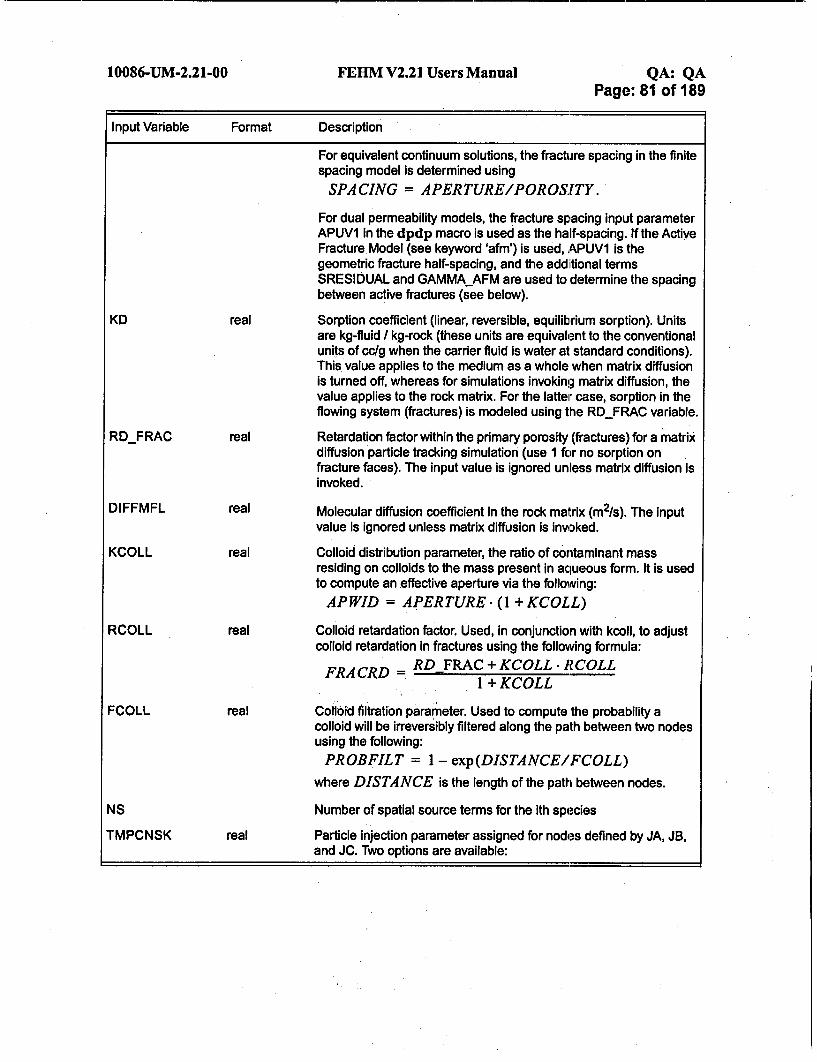
10086-UM-2.21-00 FEHM V2.21 Users Manual QA: QAPage: 81 of 189
Input Variable Format Description
For equivalent continuum solutions, the fracture spacing in the finitespacing model is determined using
SPACING = APERTURE/POROSITY.
For dual permeability models, the fracture spacing input parameterAPUV1 in the dpdp macro is used as the half-spacing. If the ActiveFracture Model (see keyword 'afm') is used, APUV1 Is thegeometric fracture half-spacing, and the addiitional termsSRESIDUAL and GAMMAAFM are used to determine the spacingbetween active fractures (see below).
KD real Sorption coefficient (linear, reversible, equilibrium sorption). Unitsare kg-fluid / kg-rock (these units are equivalent to the conventionalunits of cc/g when the carrier fluid is water at standard conditions).This value applies to the medium as a whole when matrix diffusionis turned off, whereas for simulations invoking matrix diffusion, thevalue applies to the rock matrix. For the latter case, sorption in theflowing system (fractures) is modeled using the RDFRAC variable.
RDFRAC real Retardation factor within the primary porosity (fractures) for a matrixdiffusion particle tracking simulation (use 1 for no sorption onfracture faces). The input value is ignored unless matrix diffusion isinvoked.
DIFFMFL real Molecular diffusion coefficient in the rock matrix (m2/s). The inputvalue is ignored unless matrix diffusion is invoked.
KCOLL real Colloid distribution parameter, the ratio of contaminant massresiding on colloids to the mass present in aqueous form. It is usedto compute an effective aperture via the following:
APWID = APERTURE. (1 + KCOLL)
RCOLL real Colloid retardation factor. Used, in conjunction with kcoll, to adjustcolloid retardation in fractures using the following formula:
FRACRD - RD FRAC + KCOLL. R COLL1 + KCOLL
FCOLL real Colloid filtration parameter. Used to compute the probability acolloid will be irreversibly filtered along the path between two nodesusing the following:
PROBFILT = 1 - exp(DISTANCE/FCOLL)
where DISTANCE is the length of the path between nodes.
NS Number of spatial source terms for the ith species
TMPCNSK real Particle injection parameter assigned for nodes defined by JA, JB,and JC. Two options are available:

10086-UM-2.21-OO FEHM V2.21 Users Manual QA: QAPage: 82 of 189
Input Variable Format Description
TMPCNSK > 0. - particles are injected at each node in proportion,to the source mass flow rate at the node. This boundary'condition is equivalent to injecting a solute of a givenconcentration into the system. Note: the source flow rates usedto assign the number and timing of particle injections are thoseat the beginning of the particle tracking simulation (timeDAYCS). Transient changes in this source flow rate during theparticle tracking simulation do not change the number ofparticles input to the system.
TMPCNSK < 0. - particles are introduced at the node(s),regardless of whether there is a fluid source at the node.
Default is 0. for all unassigned nodes, meaning that no particles areinjected at that node.
PINMASS real Input mass. If CONFACTOR = 0, PINMASS is the number ofparticles to be injected at locations defined by TMPCNSK. IfCONFACTOR > 0, PINMASS is the input mass expressed in moles.The code uses CONFACTOR to convert PINMASS into number ofparticles.
T1SK real Time (days) when particle injection begins. Default is 0.
T2SK real Time (days) when particle injection ends. Default is 0.
The following is an example of mptr. A multiple-species decay-chain(1 --+ 2 -- 3 - 44) is simulated, with decay half lives of the speciesequaling 10,000, 3,000, 10,000, and 4,000 years, respectively. In thissimulation a maximum of 3 property layers are specified although only Ilayer is used, the maximum number of particles is specified to be 1100100,and FEHM is run in stand-alone mode. Concentrations will be computed asnumber of particles per unit fluid volume and no output will be written tothe *.fin" file. Use of the 'zptr' keyword indicates that a single zone will bedefined for breakthrough curve output which will be written to the ".out"file. The random number seed is defined to be 244562. The particletracking solution is enabled at 0.1 days, and disabled at 3.65e8 days, whilethe flow solution is disabled at 38 days and re-enabled at 3.65e8 days.Dispersivity in the X-, Y-, and Z-directions are defined to be 0.005 m, themean fracture aperture is 0.0001 m, and the matrix porosity is 0.3.Particles for species 1 are injected at a constant rate from 0 to 5,000 years,and species 2, 3, and 4 are formed through the decay reactions, with noinput at the inlet. Advection and dispersion (without matrix diffusion) isbeing modeled. The retardation factors for the four species are 1, 1, 1.9, and1, respectively (i.e. only species 3 sorbs).
mptr4 3 1100100 0 Group 12 0 Group 2
zptrI1 1
244562 Group 30.1 3.65e8 38 3.65e8 Group 40.005 0.005 0.005 1.e-4 0.3 Group 5

10086-UM-2.21-00 FEHM V2.21 Users Manual QA: QAPage: 83 of 189
1
1000
111110000.10000.10000.10000.
10000.10000.
211110
3111
411110
0 0 1
1 3-652485E6
2 0. 1.
202 201 -10. 365365.25E2 730730.5E2 1.0,1.09575E5 1.4(
2
1 .e-14
1 -1 1. 1. 0.5
.25E2
.5E29575E531 E5
1.7532E6 1.789725E61.789725E6 1.82625E6
1 1.095745E6 3
2 0. 1. 1.e-14
202 201 -10. 1.825E6
1 3.652485E6 4
2 0.108 1. 1.e-14
202 201 -10. 1.825E6
I 1.460972E6 -1
2 0. 1. 1.e-14
202 201 -10. 1.825E6
0 -1 1. 1. 0.5
0 -1 1. 1. 0.5
0 -1 1. 1. 0.5
Group 6
Group 7Group 8Group 9Group 10Group 11Group 12Group 12Group 12Group 12
Group 12Group 12
Group 7Group 8Group 9Group 10Group 11Group 12
Group 7Group 8Group 9Group 10Group 11Group 12
Group 7Group 8Group 9Group 10Group 11Group 12
6.2.45 Control statement ngas (optional)
Noncondensible gas transport.
Group 1 - ICOD
Group 2 - JA, JB,"JC, PCO2 (JA, JB, JC - defined on page 31)
Group 3 - JA, JB, JC, CPNK (JA, JB, JC - defined on page 31)
Group 4 - JA, JB, JC, QCD (JA, JB, JC - defined on page 31)
Note that all Group 2 values are entered first, followed by Group 3 values,followed by Group 4 values.

10086-UM-2.21-00 FEHM V2.21 Users Manual QA: QAPage: 84 of 189
Input Variable Format Default Description
Input Variable Format Default DescriptionICO2D integer 3
PC02
CPNK
QCD
real
real
real
0.
0.
0.
Solution descriptor for noncondensible gas transport.IC02D = 1, the 3 degree of freedom solution will be reduced
to a 1 degree of freedom problem. (See macro Iter, theparameter ICOUPL is also set to 5 if ICO2D = 1.)
ICO2D = 2, the 3 degree of freedom solution will be reducedto a 2 degree of freedom problem. (See macro Iter, theparameter ICOUPL is also set to 5 if ICO2D = 2.)
IC02D = 3, full 3 degree of freedom.
Initial partial pressure of noncondensible gas. If PC02 < 0then ABS (PC02) is interpreted as a temperature and thepartial pressure of the noncondensible gas is calculatedaccording to the formula: PC02 = PT- PSA T() where
PT is the total pressure and PSA 7(7) is the water saturationpressure and is a function of temperature only.
If CPNK _ 0, then ABS (CPNK) is the specifiednoncondensible pressure and will be held at that value.If CPNK > 0, then CPNK is the specified relative humidity andthe saturation, SI, is calculated using the vapor pressure
lowering formula and the capillary pressure formula:Pcap(S1 ) = ln(h)p1 RT where Pcap is the capillary
function, h is the humidity, R is the gas constant, T is the
temperature, and p1 is the liquid density. Once the formula is
solved, S1 is held constant. The humidity condition is only
enabled for the van Genuchten capillary, function model. Seemacro rip.
Specified air source strength (kg/sec).
The following is an example of ngas. In this example, a full 3 degrees offreedom solution is specified. The initial temperature at nodes 1 to 800 is20 °C and the code is asked to calculate the initial nonrcondensible gaspressure. There is no specified noncondensible gas source.
ngas31 800 1 -20
1 800 1 0.
1 800 1 0.
6.2.46 Control statement nobr (optional)
Do not break connection between nodes with boundary conditions. No inputis associated with this macro.

10086-UM-2.21-OD FEHM V2.21 Users Manual QA: QAPage: 85 of 189
6.2.47 Control statement node (optional)
Specify the node numbers for which detailed output is desired.
Group I - M
Group 2- MN (1), MN (2), ... ,MN (M)
Group 3 - X, Y, Z (as needed)
or
Group 1 - KEYWORD
Group 2 - JA, JB, JC (JA, JB, JC - defined on page 31)
Input Variable Format Description
M integer Number of nodes for which information will be printed on the output(iout) and history plot (ishis, istrc) files. If M < 0, pressure andtemperature will be written on the output file for all nodes but no nodalparameter values will be printed in the history plot files. Group 2 isomitted if M <0.
MN integer M node numbers for which information will be printed on the output file(lout). If MN(I) < 0, then coordinates are used to define the print-outnode, and the coordinate sets (X, Y, Z) for each MN(I) < 0 are addedafter Group 2.
X real Coordinates of node for which information will be printed. One line foreach MN < 0. The code finds the node closest to the coordinate given.
Y real For 2-D problems set Z = 0. No input if MN >0.
Z real
KEYWORD character*5 Keyword 'block' to invoke node specification by JA, JB, JC format.
The following are examples of node. In the first example (left), 2 nodes arespecified for output, nodes 50 and 88. In the second example (center), twonodes are specified for output, the node numbered 50 and the node closestto the coordinates X = 100. m, Y = 1000, m and Z = 0. m. In the thirdexample (right), output is specified for the block of nodes 1, 11, 21, 31, 41,51, 61, 71, 81, 91 and for those nodes defined by zone :3 (see macro zone).
node2
50 88
node2
50 -88100. 1000. 0.
nodeblock
1 100 10-3 0 0
6.2.48 Control statement nod2 (optional)Specify the node numbers for which detailed file output is desired andalternate nodes for terminal output.
Group 1 - M, M2
Group 2 - MN (1), MN (2). MN (M)
Group 3 - X, Y, Z (as needed)

10086-UM-2.21-00 FEHM V2.21 Users Manual QA: QAPage: 86 of 189
Group 4 - MNI(1), MNI(2), ... , MNI(M2)
Group 5 - X, Y, Z (as needed)
Input Variable Format Description
M integer Number of nodes for which information will be printed on the output file(iout). If M <0, pressure and temperature will be written on the outputfile for all nodes but no nodal parameter values will be printed in thehistory plot files. Group 2 is omitted if M < 0.
M2 integer Number of nodes for short list (terminal printout). If M2 5 0, Group 4 isomitted.
MN integer M node numbers for which information will be printed on the output file(iout). If a MN(I) < 0, then coordinates are used to define that print-outnode, and the coordinate sets (X, Y, Z) for each MN(I) < 0 are addedafter Group 2.
MNI integer M2 node numbers for which information will be printed on the terminal(short list). This group exists only if M2 # 0. If MNI(I) < 0, thencoordinates are used to define the terminal output nodes, and thecoordinate sets (X, Y, Z) for each MNI(I) < 0 are added after Group 4.
X real Coordinates of node for which information will be printed. One line foreach MN or MNI < 0. The code finds the node closest to the coordinate
Y real given. For 2-D problems set Z = 0. No Input if no MN or MNI < 0.
Z real
The following are examples of nod2. In the first example (left), detailedoutput to the output file is specified for two nodes, the nodes numbered 50and 88, and one node is specified for terminal output, node 50. In thesecond example (right), two nodes are specified for detailed output, thenodes numbered 50 and 88, and one node is specified for terminal output,the node closest to the coordinates X = 100. m, Y = 1000. m and Z = 0. m.
nod22 1
50 88-88100. 1000. 0.
6.2.49 Control statement nod3 (optional)
Specify the node numbers for which detailed file output is desired andalternate nodes forrterminal output.
Group I - M, M2, M3
Group 2 - MN (1), MN (2) .... MN (M)
Group 3 - X, Y, Z (as needed)
Group 4 - MNI(1), MNI(2) .... MNI(M2)
Group 5 - X, Y, Z (as needed)
Group 6 - MNI(1), MNI(2), . . . , MNI(M3)

10086-UM-2.21-O0 FEHM V2.21 Users Manual QA: QAPage: 87 of 189
Group 7 - X, Y, Z (as needed)
Input Variable Format Description
M integer Number of nodes for which information will be printed on the output file(iout). If M 5 0, pressure and temperature will be written on the outputfile for all nodes but no nodal parameter values will be printed in thehistory plot files. Group 2 is omitted if M < 0.
M2 integer Number of nodes for short list (terminal printout). If M2 5 0, Group 4 isomitted.
M3 Number of nodes for short list (variable porosity model informationprintout). If M3 : 0, Group 6 is omitted.
MN integer M node numbers for which information will be printed on the output file(iout). If a MN(I) < 0, then coordinates are used to define that print-outnode, and the coordinate sets (X, Y, Z) for each MN(l) < 0 are addedafter Group 2.
MNI integer M2 node numbers for which information will be printed on the terminal(short list). This group exists only if M2 # 0. If MNI(I) < 0, thencoordinates are used to define the terminal output nodes, and thecoordinate sets (X, Y, Z) for each MNI(I) < 0 are added after Group 4.
X real Coordinates of node for which information will be printed. One line foreach MN or MNI < 0. The code finds the node closest to the coordinate
Y real given. For 2-D problems set Z = 0. No input if no MN or MNI < 0.
Z real
The following are examples of nod3. In the first example (left), detailedoutput to the output file is specified for two nodes, the nodes numbered 50and 88, and one node is specified for terminal output, node 50. In thesecond example (right), two nodes are specified for detailed output, thenodes numbered 50 and 88, and one node is specified for terminal output,the node closest to the coordinates X = 100. m, Y = 1000. m and Z = 0. m.
nod22 1
50 8850
nod22 1
50 88-88100. 1000. 0.
6.2.50 Control statement perm (required if macro hyco not used)Assign permeabilities of the rock. Permeabilities represent average valuesof a volume associated with a node. Note that using rip models 4 or 6 todescribe relative permeabilities causes these values to be overwritten.
Group 1 - JA, JB, JC, PNXD, PNYD, PNZD (JA, JB, JC - defined onpage 31)
I":;

10086-UM-2.21-0O FEHIM V2.21 Users Manual QA: QAPage: 88 of 189
Input Variable Format Default Description
PNXD real 1 .e-30 Permeability in the x-direction (m 2 ).
PNYD real 1 .e-30 Permeability in the y-direction (m 2 ).
PNZD real 1 .e-30 Permeability in the z-direction (m 2 ).
The following is an example of the perm macro. In this example, nodes 1through 140 are specified to have permeabilities in the X, Y, and Zdirections of 2.5e-14, 2.5e-14, and 0. m2 respectively.
Iperm1 140 1 2.50e-14 2.50e-14 0.00e-00
6.2.51 Control statement pest (optional)
Output variable information for PEST parameter estimation routine.
Group 1 - MPEST
Group 2 - NPEST(I), I = 1, MPEST
Group 3 - X, Y, Z (as needed)
Input Variable Format Description
MPEST integer Number of nodes for PEST output. At present the code outputs onlypressures (heads), saturations, and temperatures.
NPEST(I) integer Node numbers printed to the output file (fehmn.pest) with values ofvariables listed above. If NPEST(I) < 0 then the node numbers aredetermined from the coordinates.
X, Y, Z real Coordinates in grid if NPEST(I) < 0. The coordinates are used to findthe node closest in distance to that point and that node is substitutedfor NPEST(I).
The following is an example of pest. In this example pest output isspecified at 5 nodes, nodes numbered 21, 23, 35, and 47, and the nodeclosest to the coordinates X=10. m, Y=15. m, Z=20. m.
pest21 23 35 47 -5010. 15. 20.
6.2.52 Control statement ppor (optional)
Group 1 - IPOROS
Group 2 - JA, JB, JC, PORI, POR2, POR3, POR4 (number of parametersentered depends on model type) (JA, JB, JC - defined onpage 31)

10086-UM-2.21-00 FEHM V2.21 Users Manual QA: QAPage: 89 of 189
Input Variable Format Description
IPOROS integer
Model (1): IPOROS = 1,
PORI real
Model (-1): IPOROS = -1,
PORI real
Model (-2): IPOROS = -2,
Model type:IPOROS = 1, aquifer compressibility modelIPOROS = -1, specific storage model (use only for isothermal
conditions)IPOROS = -2, Gangi model (not available for air-water-heat conditions)
Aquifer compressibility • = + a (P - Po)where
aa = aquifer compressibility (MPa"1)
00 = initial porosity
P0 = initial pressure (MPa)
Aquifer compressibility (X (MPa"1)
Specific storage S. = pg(,a + 0 0)where
p = liquid density (kg/m 3)
g= gravity
aa = aquifer compressibility (MPa"1)
= porosity
=J liquid compressibility (MPa"1)
Specific storage S. (m"1)
Gangi model with calculation of initial permeability and porosity.
0 = 00[i1- Pc) m and PC = a-P-(xE(T- TO)
where
0= initial porosity
m = Gangi exponent
Px= fitted parameter (MPa)
Y = in-situ stress (MPa)
a = coefficient of thermal expansion (1/C)
E = Young's modulus (MPa)
T = temperatures (0C)
To = initial temperature (0C)
Note: for the Gangi model the permeability is varied by k =
Exponent m in Gangi bed of nails model.PORI
POR2
realreal Px parameter (MPa) in Gangi equation.

10086-UM-2.21-00 FEHM V2.21 Users Manual QA: QAPage: 90 of 189
Input Variable Format Description
POR3 real a in-situ stress (MPa).
POR4 real (aE) The product of the coefficient of thermal expansion for the rock
and the Young's modulus (MPa/°C).Note: For isothermal simulations the thermal term does not apply.
In the following example of ppor, aquifer compressibility is modeled. Allnodes In the model are assigned a compressibility of L.e-2 MPa"1 .
6.2.53 Control statement pres (required if macro init not used)
Group 1 - JA, JB, JC, PHRD, TIND, IEOSD (JA, JB, JC - defined onpage 31)
The initial values defined in control statement pres supersede all others.Note that the term "saturated" refered to In IEOSD, Is not thegroundwater hydrology definition (volumetric fraction of pore void that Isfilled with water) used elsewhere in this document. Saturated hereindicates that vapor and liquid phases exist simultaneously. Thesuperheated region means that all pore space is filled with gas.
Input Variable Format Default Description
PHRD real PEIN Initial pressure (MPa).
TIND real Initial temperature (°C) if IEOSD = 1 or 3,Initial saturation if IEOSD = 2
IEOSD integer 1 Thermodynamic region parameter.IEOSD = 1, the compressed liquid regionIEOSD = 2, the saturation regionIEOSD = 3, the superheated region.
If IEOSD < 0 then the code uses ABS (IEOSD) and fixesthe values of PHRD and TIND to the values providedabove.
The following is an example of pres. In this example, zones numbered 1, 2,3, 4. 5 and 6, and nodes 1 through 800 have an Initial pressure of 0.1 MPaand are located in the saturation region. The Initial water saturation forzones 1, 2, and 4 Is 0.1, for zone 3 is 0.003, for zones 5 and 6 is 0.11, and fornodes I through 800 is 0.5. In addition, for zone 6 the pressure andsaturation are held constant throughout the run.

10086-UM-2.21-00 FEHM V2.21 Users Manual QA: QAPage: 91 of 189
pres-1 0 1 0.1 0.1 2-2 0 1 0.1 0.1 2-3 0 1 0.1 0.003 2-4 0 1 0.1 0.1 2-5 0 1 0.1 0.11 2-6 0 1 0.1 0.11 -21 800 1 0.1 0.5 2
6.2.54 Control statement ptrk (optional, cannot be used with trac)
Particle tracking simulation input. Note that data for each numberedgroup must be input. The other input is optional.
Group 1 - NPART, RSEED
KEYWORD 'rip'
Group 2 - DAYCS, DAYCF, DAYHF, DAYHS
or if the optional keyword 'rip' follows Group 1
Group 2 - DAYCS, DAYCF, DAYHF, DAYHS, RIPFEHM, CONFREAD,GMOL, P-FRACTION
Group 3 - TRAKTYPE, HALFLIFE, POUT, PRNT_.RST
Optional keyword "tcurve" is input to indicate that transfer function curvesshould be input to model matrix diffusion. It is followed by NUMPARAMSand TFILENAME.
KEYWORD
NUMPARAMS
TFILENAME
Optional keyword "zptr" designates zones for breakthrough curves will bedefined. It is followed by IPZONE and IDZONE.
KEYWORD 'zptr'
IPZONE
IDZONE(I) I = I to IPZONE
Group 4 is used to define models in which identical sorption and transportparameters are assumed to apply. Group 4 data are read until a blank lineis encountered. The model number ITRC is incremented by 1 each time aline is read. Model parameters defined in Group 4 are assigned to nodes orzones using Group 5.
An optional, flexible input structure involving the assignment of transportparameters is inlplemented in the particle tracking input to allow multiplerealization simulations to use different parameters for each realization.The user invokes this option using the keyword 'file' before Group 4,followed by the name of the file that the transport parameters reside in.
KEYWORD 'file'
PFILENAME
The structure of the alternate parameter file is:

10086-UM-2.21-00 FEHM V2.21 Users Manual QA: QAPage: 92 of 189
NINPUTSheading or blank linePTRPARAM(I) I=I to NINPUTS
[a line of parameters is present for each realization]
The method for assigning a given value of PTRPARAM to a specifictransport parameter, defined in Group 4, is discussed below. There are anarbitrary number of input lines each representing a given realization ofparameter value•s2 In a multiple-realization scenario, the code enters theinput file for each realization, and for this input, reads down thecorresponding number of lines to obtain the parameters for thatrealization. For example, for realization number 10, the code reads down tothe 10th line of data (line 12 in the file) and uses those parameter values.
Once these parameters are read in for a given realization, they must beassigned to specific transport parameters. This is done in the following wayIn Group 4. If any of the inputs other than TRANSFLAG are negative, thecode takes the absolute value of the number and interprets it as the columnnumber from which to assign the transport parameter. For example, ifDIFFMFL = -5, then the diffusion coefficient is the fift:h input number inthe PTRPARAM array. In this way, any of the transport parameter Inputscan be assigned through the alternate input file rather than the input linein ptrk.
There are four possible forms of input for Group 4, which depend onwhether or not the Active Fracture Model is implemented (optionalKEYWORD 'afm') and colloid transport Is enabled (TRANSFLAG < 0). Ifcolloid transport is enabled, then ABS(TRANSFLAG) is used to determinethe transport mechanism. Note that optional KEYWORD 'size' is only usedwhen colloid transport is enabled.
KEYWORD 'afm'
KEYWORD 'size'
PARTSIZE(I), PROBSIZE(I) - an arbitrary numbers of lines ofInput, terminated by a blank line.
If there is no colloid transport, TRANSFLAG > 0
Group 4 - TRANSFLAG(ITRC), KD(ITRC), TCLX(ITRC), TCLY(ITRC),TCLZ(ITRC), DIFFMAT(ITRC), RDFRAC(ITRC),MATRIX POR(ITRC), APERTURE(ITRC)
or when 'afm' is implemented without colloid transport
Group 4 - TRANSFLAG(ITRC), KD(ITRC), TCLX(ITRC), TCLY(ITRC),TCLZ(ITRC), DIFFMAT(ITRC), RDFRAC(ITRC),MATRIXPOR(ITRC), APERTURE(ITRC), SRESIDUAL(ITRC),GAMMAAFM(ITRC)
or when colloid transport is enabled, TRANSFLAG < 0
Group 4 - TRANSFLAG(ITRC), KD(ITRC), TCLX(ITRC), TCLY(ITRC),TCLZ(ITRC), DIFFMAT(ITRC), RDFRAC(ITRC),MATRIXPOR(ITRC), APERTURE(ITRC), KCOLL(ITRC),RCOLL(ITRC), FCOLL(ITRC)

10086-UM-2.21-00 FEHM V2.21 Users Manual QA: QAPage: 93 of 189
or when 'afm' is implemented with colloid transport
Group 4 - TRANSFLAG(ITRC), KD(ITRC), TCLX(ITRC), TCLY(ITRC),TCLZ(ITRC), DIFFMAT(ITRC), RDFRAC (ITRC),MATRIXPOR(ITRC), APERTURE(ITRC), KCOLL(ITRC),RCOLL(ITRC), FCOLL(ITRC), SRESIDUAL(ITRC),GAMMAAFM(ITRC)
Group 5 - JA, JB,;JC, ITRC (JA, JB, JC - defined on page 31)
Group 6 - JA, JB, JC, PCNSK, T1SK, T2SK (JA, JB, JC - defined onpage 31)
If POUT = 5, an additional Group is included at the end of the ptrk input
Group 7 - JA, JB, JC, NODEPCONC (JA, JB, JC - defined on page 31)
The concentration output is written to the .trc", %.out", and AVSconcentration output files. The ".fin" file is used only when specified (a non-zero value is input for PRNTRST).
Input Variable Format Description
NPART integer Number of particles in the simulation. Note: the actual number may beslightly less than the number specified by the user because when thecode divides the particles among the starting nodes as specified inGroup 7, the code must input an integer number of particles at eachnode.
RSEED integer 6-digit integer random number seed.
KEYWORD character*4 Optional keyword 'rip' designating this is a GoldSim coupled simulationand the alternate Group 2 data format should be used.
DAYCS real Time which the particle tracking solution is enabled (days).
DAYCF real Time which the particle tracking solution is disabled (days).
DAYHF real Time which the flow solution is disabled (days).
DAYHS real Time which the flow solution is enabled (days).
RIPFEHM integer Parameter for assigning the particle starting locations based onradionuclide flux input from the computer code GoldSim. Used whenGoldSim is the driver program and FEHM is dynamically linked toperform particle tracking transport.
If RIPFEHM = 1 Use input from GoldSim to assign particle startinglocations.
If RIPFEHM •1 Assign starting locations in the normal way.
CONFREAD real Initial conversion factor for GoldSim-FEHM coupling(# of particles/mole).
If CONFREAD=O, at each time step, the code selects a conversionfactor based on the available memory and the remaining simulationtime (end time - current time). The code then uses the selectedconversion factor to calculate the number of particles to be injectedat the current time step.
If CONFREAD >0, the code uses the product of the CONFREAD andthe input mass (in moles) to calculate the input number of particlesat each time step.

10086-UM-2.21-00 FEHM V2.21 Users Manual QA: QAPage: 94 of 189
Input Variable Format Description
GMOL real The molecular weight of the ith species. The code uses GMOL andCONFREAD to convert the mass from number of particles to grams inthe final output.
PFRACTION real The decay-ingrowth particle release factor (percentage of themaximum number of particles released for the parent species). Valuesare in the range 0. - 1. If the value is omitted it will default to 0.5.
TRAKTYPE integer Flag to denote the fluid phase of the particles:1 - liquid phase particles2 - vapor phase particles
HALFLIFE real Half-life for irreversible first order decay reaction (s). SetHALFLIFE = 0 for no decay.
POUT integer Flag to specify the concentration output:0 - Concentration output is a running total of the number of particles
which have left each node, divided by the fluid or vapor mass atthat node depending on traktype.
1 - Concentrations computed as number of particles per unit totalvolume (rock and fluid)
2 - Concentrations computed as number of particles per unit fluidvolume (the fluid is liquid for TRAKTYPE = 1 and gas forTRAKTYPE = 2).
3 - Concentrations computed as number of particles at a given nodepoint.
5 - If this option is invoked, the particles injected at a particular nodeare assigned concentrations according to the input concentrationdefined in the NODEPCONC array (Group 7). The code thenoutputs the mixed mean concentration at each node in the modelbased on the assumption of steady state flow.
6 - Used for C-14 radioactive decay particle mixing model (only liquidtracer). For meaningful results the particles must all be injectedsimultaneously in a pulse (give a very short duration of injectionstarting at time 0). The code contains data describing the functionf(t) vs. time where f(t) is given as:
J exp(-kt)dt0
where t is the time the particle enters the system and k is theradioactive decay constant for C-14. The output Is the finalconcentration afterall the particles have left the system.
-1, -2, -3, or -6 - Concentrations ormputed as specified above forabs(pout). The .trc file contains breakthrou:gh output for the firstnode specified in the node macro.
-7 -Output is written every time a particle leaves a cell. This output isparticle number, cell number that the particle Is leaving, zonenumber of the cell, and time the particle leaves the cell.

10086-UM-2.21-00 FEHM V2.21 Users Manual QA: QAPage: 95 of 189
Input Variable Format Description
PRNT_RST integer Flag to specify whether particle information is written to the *.fin" file:0 - Particle information is not written to Afin" file.1 - Particle information is written to the ".fin" file.2 - Mass flux values are written to the ".fAn" file followed by particle
information.-1 - Particle positions and ages only are written to the "fin" file.-2 - Mass flux values are written to the ".fin" file followed by particle
positions and ages only.
When particle tracking data or mass fluxes are written to the *.fin" file,the arrays are written after all of the heat and mass simulationinformation. The mass fluxes can be read into the code In asubsequent ptrk or mptr simulation and the code can simulatetransport on this steady state flow field (see macro rflo).The particleinformation written is sufficient to perform a restart of the particletracking simulation and to post-process the data to compile statisticson the particle tracking run. However, for a large number of particles,this file can become quite large, so particle tracking information shouldonly be written when necessary. Thus, 0 should be used forPRNTRST unless restarting or post-processing to obtain particlestatistics is required. Selecting the -1 option allows a subset of the fullset of information needed for a restart (particle positions and ages) tobe written. Restart runs that use this file as input will only beapproximate, since the particle is assumed to have just entered itscurrent cell. For restart runs, PRNTRST = 1 is preferred, whilePRNTRST = -1 is appropriate for output of particle statistics for post-processing.
KEYWORD character Optional keyword "tcurve" indicating transfer function curve data shouldbe input to model matrix diffusion. If the keyword is found thenNUMPARAMS and FILENAME are entered, otherwise t~hey areomitted.
NUMPARAMS
TFILENAME
integer Number of parameters that define the transfer function curves beingused.
character Name of input file containing the transfer function curve data.
KEYWORD character*4 Optional keyword 'zptr' designating zones for breakthrough curves willbe defined. If no keyword is input, IPZONE and IDZONE are alsoomitted.
IPZONE
IDZONE
integer
integer
Number of zones for which breakthrough curves are to be output
A list of zones for which particle breakthrough data are required.The code outputs the number of particles that leave the system ýt eachzone IDZONE at the current time step. This information Is written to the".out" file at each heat and mass transfer time step.ý
Optional keyword 'file' designating alternate transport parameter fileinput for multiple simulation realizations.
Name of file from which to read transport parameters.
KEYWORD character*4
PFILENAME character*80

10086-UM-2.21-OO FEJM V2.21 Users Manual QA: QAPage: 96 of 189
Input Variable Format Description
NINPUTS
PTRPARAM
integer
real
Number of inputs in each row of data in the alternate transportparameter input file (PFILENAME).
Array of transport parameter values in the alternate transportparameter input file (PFILENAME). The parameters that may be inputare those entered for Group 4. Only those parameters being changedat each realization need be entered.
KEYWORD character*4 Optional keyword 'afm' designating the Active Fracture Model input fordetermining fracture spacing should be used.
KEYWORD
PARTSIZE
character*4 Optional keyword 'size' designating that the colloid size distributionmodel option is being used (combined with the Interface filtration optionin the ltfc macro). If the keyword is not input, PARTSIZE andPROBSIZE are also omitted.
real
PROBSIZE real
TRANSFLAG integer
Colloid particle size for this entry of the particle size distribution table(paired with a value of PROBSIZE). An arbitrary number of entries canbe input, terminated with a blank line. The code assigns each particle asize based on this distribution of particle sizes, and decides if particlesare irreversibly filtered based on the pore size distribution assigned inthe itfc macro.
Colloid cumulative probability for the distribution of sizes (paired with avalue of PARTSIZE). See description of PARTSIZE above for details.The final entry of the table must have PROBSIZE = 1, since thedistribution is assumed to be normalized to unity.
Flag to~specify which transport mechanisms apply[abs(TRANSFLAG)]:
1 - advection only (no dispersion or matrix diffusion)2 - advection and dispersion (no matrix diffusion)3 - advection and matrix diffusion, infinite fracture spacing solution
(no dispersion)4 - advection, dispersion, and matrix diffusion, Infinite fracture
spacing solution5 - advection and matrix diffusion, finite fracture spacing solution (no
dispersion)6 - advection, dispersion, and matrix diffusion, 'finite fracture spacing
solution8 - use the the transfer function approach with 3 dimensionless
parameters and type curves for handling fracture-matrixinteractions.
For TRANSFLAG < 0, transport simulations include colloids.
For equivalent continuum solutions, the fracture spacing in the finitespacing model is determined using
SPACING = APERTURE/POROSITY.
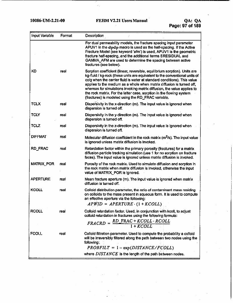
10086-UM-2.21-00 FEHM V2.21 Users Manual QA: QAPage: 97 of 189
Input Variable Format Description
For dual permeability models, the fracture spacing input parameterAPUV1 in the dpdp macro is used as the half-spacing. If the ActiveFracture Model (see keyword 'afm') is used, APUV1 is the geometricfracture half-spacing, and the additional terms SRESIDUAL andGAMMAAFM are used to determine the spacing between activefractures (see below).
KD real Sorption coefficient (linear, reversible, equilibrium sorption). Units arekg-fluid / kg-rock (these units are equivalent to the conventional units ofcc/g when the carrier fluid is water at standard conditions). This valueapplies to the medium as a whole when matrix diffusion is turned off,whereas for simulations invoking matrix diffusion, the value applies tothe rock matrix. For the latter case, sorption in the flowing system(fractures) is modeled using the RDFRAC variable.
TCLX real Dispersivity in the x-direction (m). The input value is ignored whendispersion is turned off.
TCLY real Dispersivity in the y-direction (m). The input value is ignored whendispersion Is turned off.
TCLZ real Dispersivity in the z-direction (m). The input value is ignored whendispersion is turned off.
DIFFMAT real Molecular diffusion coefficient in the rock matrix (m2/s). The Input valueis ignored unless matrix diffusion is invoked.
RDFRAC real Retardation factor within the primary porosity (fractures) for a matrixdiffusion particle tracking simulation (use I for no sorption on fracturefaces). The input value is ignored unless matrix diffusion is invoked.
MATRIXPOR real Porosity of the rock matrix. Used to simulate diffusion and sorption inthe. rock matrix when matrix diffusion is invoked, otherwise the inputvalue of MATRIXPOR is ignored.
APERTURE real Mean fracture aperture (m). The input value is ignored when matrixdiffusion is turned off.
KCOLL real Colloid distribution parameter, the ratio of contaminant mass residingon colloids to the mass present in aqueous form,, It is used to computean effective aperture via the following:
APWID = APERTURE. (I + KCOLL)
RCOLL real Colloid retardation factor. Used, in conjunction with kcoll, to adjustcolloid retardation in fractures using the followingformula:
RA CRD = RD FRAC + KCOLL RCOLL1 + KCOLL
FCOLL real Colloid filtration parameter. Used to compute the probability a colloidwill be irreversibly filtered along the path between two nodes using thefollowing:,
PROBFILT = 1 - exp(DISTANCE/FCOLL)where DISTANCE is the length of the path between nodes.

10086-UM-2.21-00 FEHM V2.21 Users Manual QA: QAPage: 98 of 189
Input Variable Format Description
SRESIDUAL real ResidUal saturation in the Active Fracture Model used for determiningthe spacing between active fractures. This parameter Is only neededwhen the keyword 'afm' is included, in which case the input must beentered. However, the model is only used in dual permeabilitysimulations at locations where the finite spacing matrix diffusion modelIs invoked [abs(TRANSFLAG) = 5 or 6].
GAMMAAFM real Exponent in the Active Fracture Model used for determining thespacing between active fractures. See comments for SRESIDUALabove.
ITRC integer Model number for parameters defined in group 4. Default is 1.PCNSK real Particle injection parameter assigned for nodes defined by JA, JB, and
JC. When multiple lines of input are given for Group 6, all PCNSKvalues must have the same sign (i.e. the two options, described below,cannot be invoked in the same simulation).
PCNSK > 0 - particles are injected at each node in proportion to thesource mass flow rate at the node. When multiple lines of inputare given for Group 6, PCNSK is proportional to the particleinjection concentration. This boundary condition is equivalent toinjecting a solute of a given concentration into the system. Note:the source flow rates used to assign the number and timing ofparticle injections are those at the beginning of the particletracking simulation (time DAYCS). Transient changes in thissource flow rate during the particle tracking simulation do notchange the input of particles to the system.
PCNSK < 0 - particles are introduced at the node(s), regardless ofwhether there is a fluid source at the node. When multiple lines ofinput are given for Group 6, abs(PCNSK) is proportional to thenumber of particles introduced at the node(s).
Default is 0 for all unassigned nodes, meaning that no particles areinjected at that node.
TI SK real Time (days) when particle injection begins. Default is 0.T2SK real Time (days) when particle injection ends. Default is 0.
NODEPCONC real Input particle concentrations. The concentration associated with aparticle entering the system at a specified node.
Notes on Restarting: As with all restart runs for FEHM, a *.ini" file isspecified to be read to set the initial conditions upon restarting. However,there are two possibilities for restart calculations with particle tracking:1) the heat and mass transfer solution is being restarted, but the particletracking simulation is initiated during the restart run (it was not carriedout in the simulation that generated the ".ini" file); or 2) the heat and masstransfer solutionand the particle tracking simulation are both beingrestarted. If the,.code does not find the "ptrk" key word at the top of the".ini" file, then týe original run did not employ particle tracking, and Case1 is assumed. A common example is a preliminary calculation thatestablishes a fluid flow steady state, followed by a restart simulation oftransport.

10086-UM-2.21-00 FEHM V2.21 Users Manual QA: QAPage: 99 of 189
If "ptrkW was written into the ".ini" file in the original run, the particle datain the ".ini" file are read and used to initialize the particle trackingsimulation (Case 2). In this instance, the number of particles (NPART)must be set the same for the restart run as in the original run or theresults will be unpredictable.When restarting a particle trackingsimulation, certain input data are overwritten by information in the ".ini"file. These parameters include RSEED, PCNSK, T1SK, and T2SK. Otherinput parameters can be set to different values in the restart run than theywere in the original run, but of course care must be taken to avoidphysically unrealistic assumptions, such as an abrupt change in transportproperties of Group 4 part way through a simulation.
A final note on restart calculations Is in order. A common technique inFEHM restart calculations is to reset the time at the top of the ".ini" file to0, so that the starting time of the restart simulation is arbitrarily 0, ratherthan the ending time of the original simulation. This is useful for theexample of the steady state flow calculation, followed by a restart solutetransport calculation. Although this technique is acceptable for particletracking runs that are initiated only upon restart (Case 1), it is invalidwhen a particle tracking run is being resumed (Case 2). The reason is thatall particle times read from the ".ini" file are based on the starting time ofthe original simulation during which the particle tracking simulation wasinitiated.
The following is an example of ptrk:
ptrk100000 12294510. 20. 10. 20.1 0 2 04 0. 2. 2. 2. 5.e-11 1. 0.1 0.3334 3. 2. 2. 2. 1.e-10 1. 0.28 2.
1 0 0 1-2 0 0
-3 0 0 1. 10. 10.0001
In this example, 100,000 nondecaying, liquid-borne particles areintroduced as a sharp pulse (from time 10 to 10.0001 clays) with theinjection fluid in zone 3 (an injection well defined in the zone macropreceding ptrk). The particle tracking simulation starts as the heat andmass transfer simulation is turned off at day 10, after having established afluid flow steady state. Two models are defined for assigning transportproperties of the particles. All nodes are assigned to model 1, after whichmodel 2 properties are assigned for zone 2. A combined-advection,dispersion, and matrix diffusion model is used for all nodes. However,sorption in the matrix occurs only for model 2 (which is zone 2 in thissimulation), and the matrix transport properties (porosity, fracturespacing, diffusion coefficient) differ for this model as well.

10086-UM-2.21-00 FEHM V2.21 Users Manual QA: QAPage: 100 of 189
6.2.55 Control statement renu (optional)
Renumbers the nodes. This option should only be used by someone familiarwith the linear equation solver routines and grid renumbering techniques.
Group 1 - IIRB(I) I = 1, NEQ
Input Variable Format Descriptione
IIRB integer New node number for given node. A value is entered for each node.
6.2.56 Control statement rflo (optional)
This option is available for single continuum or double porosity/doublepermeability (dpdp) models only. No input is associated with this macro.
When invoked, the code will read mass flux values (kg/si from the ".ini" file.Mass flux values are read for each connection of each node, starting withnode 1. The mass flux values include sources and sinks for each node. Flowinto a node Is negative, and flow out of a node is positive. The mass fluxvalues for the fracture domain are read first followed by the mass fluxvalues in the matrix domain. The mass flux between fracture and matrixelements are read last. Flow from the fracture to the matrix is denoted aspositive.
Mass flux values can be generated during a previous FEHM particletracking simulation (see macro ptrk) or may be generated by an alternateflow code (see Ho, 1997).
6.2.57 Control statement rip (optional)
Relative permeability and capillary pressure model. Several models areavailable.
Group 1 - IRLP(i), RP1, RP2, RP3, RP4, RP5, RP6, RP7, RP8, RP9, RP10,RP 11, RP12, RP13, RP14, RP15, RP16 (number of parametersentered depends on model selected)
Group 2 - JA, JB, JC, I (JA, JB, JC - defined on page 31)
Only those parameters defined for a given model need to be input. Group 1is ended when a blank line is encountered. The parameter i is incrementedeach time a Group 1 line is read. Group 2 lines will refer to this parameter.For model number 4 (the combined van Genuchten model), thepermeability is isotropic and overwrites the input from macro perm.
Input Variable Format Description
IRLP(i) integer Relative permeability model type.
Model -1: IRLP(i) = -1, constant relative permeability, linear capillary pressure (4 parameters required).
RP1 real Liquid relative permeability (m 2 ).
RP2 real Vapor relative permeability (m 2 ).
RP3 real Capillary pressure at zero saturation (MPa).
RP4 real Saturation at which capillary pressure goes to zero.

10086-UM-2.21-OD FEHM V2.21 Users Manual QA: QAPage: 101 of 189
Input Variable Format Description
Model 1:
RP1
RP2
RP3
RP4
RP5
RP6
Model 2:
RP1
RP2
RP3
RP4
IRLP(i) = 1, linear relative permeability, linear capillary pressure (6 parameters required).
real Residual liquid saturation.
real Residual vapor saturation.
real Maximum liquid saturation.
real Maximum vapor saturation.
real Capillary pressure at zero saturation (MPa).
real Saturation at which capillary pressure goes to zero.
IRLP(i) = 2, Corey relative permeability, linear capillary pressure (4 parameters required).
real Residual liquid saturation.
real Residual vapor saturation.
real Capillary pressure at zero saturation (MPa).
real Saturation at which capillary pressure goes to zero.
Model 3: IRLP(i) = 3, van Genuchten relative permeability, van Genuchten capillary pressure (6parameters required). In this model permeabilities are represented as a function of capillarypressure [rlp(h)].
RP1 real
RP2 real
RP3 real
RP4
RP5
real
real
Residual liquid saturation.
Maximum liquid saturation.
Inverse of air entry head, oxG (1/m) [note some data is given in(1/Pa) convert using pressure = pgAh].Poweri'n in van Genuchten formula.
Low saturation fitting parameter, multiple of cutoff capillary pressureassigned as maximum capillary pressure.
If RP5 < 0 then a linear fit from the cutoff saturation (RP6) is used.The slope of the cutoff saturation is used to extend the functionto saturation = 0.
If RP5 = 0, a cubic fit is used. The slope at the cutoff saturation is
matched and the conditions -Pcap = 0 and cap = 0
are forced at S = 0.If RP5 > 0, a multiple of the value of the capillary pressure at the
cutoff saturation, RP5 * Pcap(Scjoff) is forced at S = 0.
Cutoff saturation used in fits described for RP5, must be greater thanRP1.
RP6 real

10086-UM-2.21-00 FEHIM V2.21 Users Manual QA: QAPage: 102 of 189
Input Variable Format Description
Model 4: IRLP(i) = 4, van Genuchten relative permeability, van Genuchten capillary pressure, effectivecontinuum (15 parameters required). In this model permeabilities are represented as afunction of capillary pressure [rlp(h)].
RP1 real Residual liquid saturation, matrix rock material.
RP2 real Maximum liquid saturation, matrix rock material.
RP3 real Inverse of air entry head, OCG (1/m) [note some data is given in(1/Pa) convert using pressure = pgAh], matrix rock material.
RP4 real Power n in van Genuchten formula, matrix rock material.
RP5 real Low saturation fitting parameter, matrix rock material, multiple ofcutoff capillary pressure assigned as maximum capillary pressure.
If RP5 < 0 then a linear fit from the cutoff saturation (RP6) is used.The slope of the cutoff saturation is used to extend the functionto saturation = 0.
If RP5 = 0, a cubic fit is used. The slope at the cutoff saturation isa2
matched and the conditions -cap = 0 and -- Pcap = 0
are forced at S = 0.If RP5 > 0, a multiple of the value of the capillary pressure at the
cutoff saturation, RP5 e Pcap(SCtoff) is forced at S = 0.
RP6 real Cutoff saturation used in fits described for RP5, must be greater than
RPII.
RP7 real Residual liquid saturation, fracture material.
RP8 real Maximum liquid saturation, fracture material.
RP9 real Inverse of air entry pressure, aG (1/m) [note some data is given in(1/Pa) convert using pressure = pgAh], fracture material.
RPIO real Power n in van Genuchten formula, fracture material.
RP1 1 real Low saturation fitting parameter, fracture material, multiple of cutoffcapillary pressure assigned as maximum capillary pressure.
If RP1 1 < 0 then a linear fit from the cutoff saturation (RP12) isused. The slope of the cutoff saturation is used to extend thefunction to saturation = 0.
If RP11 = 0, a cubic fit is used. The slope at the cutoff saturation isa a2matched and the conditions 0cap = and -a-•Pcap = 0
are forced at S = 0.If RP1 1 > 0, a multiple of the value of the capillary pressure at the
cutoff saturation, RPI 1 e Pcap(SCutoff) is forced at S = 0.

10086-UM-2.21-00 FEHM V2.21 Users Manual QA: QAPage: 103 of 189
Input Variable Format Description
RP12 real Cutoff saturation used In fits described for RP1 1, must be greaterthan RP7.
RP13 real Fracture permeability (m2). This is the permeability of the individualfractures. The bulk permeability of the fracture continuum isRPi3 xRP15.
RP14 real Matrix rock saturated permeability (m2 ).
RP15 real Fracture volume fraction.
Model 5: IRLP(i) = 5, van Genuchten relative permeability, van Genuchten capillary pressure (6parameters required). This model and its input are the same as for Model 3 except thatpermeabilities are represented as a function of saturation [rip(S)] rather than capillarypressure.
Model 6: IRLP(i) = 6, van Genuchten relative permeability, van Genuchten capillary pressure, effectivecontinuum (15 parameters required). This model and its input are the same as for Model 4except that permeabilities are represented as a function of saturation [rip(S)] rather thancapillary pressure.
Model 7: IRLP(i) = 7, van Genuchten relative permeability, van Genuchten capillary pressure, effectivecontinuum with special fracture interaction term '(16 parameters required). This model and itsinput are the same as for Model 6 except that the an additional term is included whichrepresents the fracture-matrix interaction.
RP16 real Fracture-matrix interaction term. If RP16 < 0, then an additionalmultiplying term equal to the relative permeability is applied to thefracture-matrix interaction term for dual permeability problems. IfRP16 >0, then an additional multiplying term equal to sI**RP16and (1. -sl)**RP16 Is applied to the fracture-matrix interactionterms for the liquid and vapor phases, respectively, for dualpermeability problems. Here, sl is the value of saturation at thegiven node.
Model 10: IRLP(i) = 10, linear relative permeability with minimum relative permeability values, linearcapillary pressure (8 parameters required).
RP1 real Residual liquid saturation.
RP2 real Residual vapor saturation.
RP3 real Maximum liquid saturation.
RP4 real Maximum vapor saturation.
RP5 real Minimum liquid permeability (m2).
RP6 real Minimum vapor permeability (m2 ).
RP7 real Capillary pressure at zero saturation (MPa).
RP8 real Saturation at which capillary pressure goes to zero.RP8 real Saturation at which capillary pressure goes to zero.

10086-UM-2.21-00 FEHM V2.21 Users Manual QA: QAPage: 104 of 189
The following is an example of rip. In this example, Corey type relativepermeability is specified, with residual liquid saturation of 0.3, residualvapor saturation of 0.1, a base capillary pressure of 2 MPa, and capillarypressure goes to zero at a saturation of 1. This model is assigned to nodesnumbered 1 through 140.
6.2.58 Control statement rock (required)
Assign rock density, specific heat and porosity.
Group I - JA, JB, JC,.DENRD, CPRD, PSD (JA, JB, JC - defined onpage 31)
Input Variable Format Description
DENRD real Rock density (kg/m 3).CPRD real Rokseii et(MJ
relRock specific heat ( . If CPRD > 1 the code will assume the
units are ( gJ. K ) and multiply by 10-6.
PSD real Porosity.Special note on negative porosities. If the code encounters anegative porosity, the node at which the negative porosity occurs iseffectively removed from the model. That is, the geometricconnections from that node to other nodes in the model areremoved. The volume associated with the node acts as a barrier toflow. For input purposes, the node may still be assigned properties,though they will have no effect on the simulation results.
The following is an example of rock. In this example the nodes numbered 1through 140 are assigned a rock density of 2563. kg/m3 , a rock specific heatof 1010. J/(kg K) and a porosity of 0.35.
1r• 140. 1 2563. 1010. 0.5
6.2.59 Control statement rxn (optional)
Chemical reactions between components are invoked with this controlstatement. It is used in conjunction with control statement trac. Forfacilitating the construction of the rxn input, a header describing the inputis required before each group whether data is entered for that group or not(see examples) unless otherwise noted. The header is an arbitrary textstring that must be contained on a single line. Note that for componentsthat do not react with other components, rxn is unnecessary. Specifically,conservative tracers or tracers that follow the equilibrium sorption
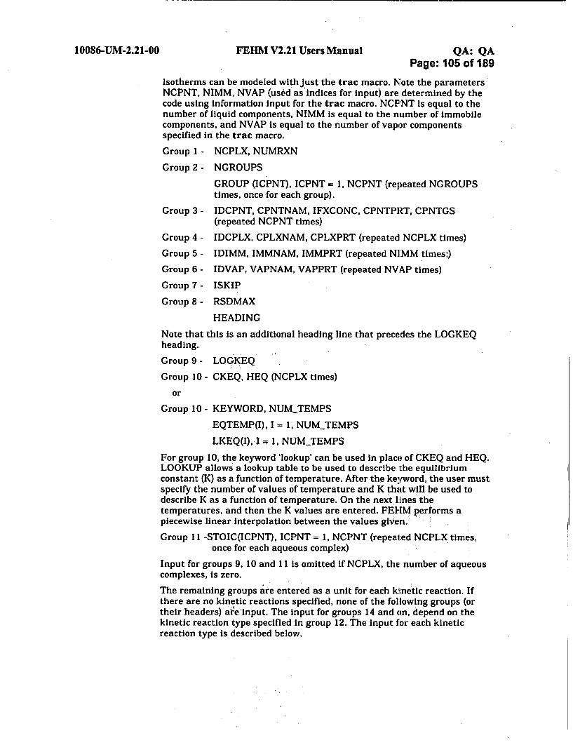
10086-UM-2.21-00 FEHM V2.21 Users Manual QA: QAPage: 105 of 189
isotherms can be modeled with Just the trac macro. Note the parametersNCPNT, NIMM, NVAP (used as indices for input) are determined by thecode using information input for the trac macro. NCPNT is equal to thenumber of liquid components, NIMM is equal to the number of immobilecomponents, and NVAP is equal to the number of vapor componentsspecified in the trac macro.
Group 1 - NCPLX, NUMRXN
Group 2 - NGROUPS
GROUP (ICPNT), ICPNT = 1, NCPNT (repeated NGROUPStimes, once for each group).
Group 3 - IDCPNT, CPNTNAM, IFXCONC, CPNTPRT, CPNTGS(repeated NCPNT times)
Group 4 - IDCPLX, CPLXNAM, CPLXPRT (repeated NCPLX times)
Group 5 - IDIMM, IMMNAM, IMMPRT (repeated NIMM times;)
Group 6 - IDVAP, VAPNAM, VAPPRT (repeated NVAP times)
Group 7 - ISKIP
Group 8 - RSDMAX
HEADING
Note that this is an additional heading line that precedes the LOGKEQheading.
Group 9- LOGKEQ
Group 10 - CKEQ, HEQ (NCPLX times)
or
Group 10 - KEYWORD, NUMTEMPS
EQTEMP(I), I = 1, NUMTEMPS
LKEQ(I), I = 1, NUMTEMPS
For group 10, the keyword 'lookup' can be used in place of CKEQ and HEQ.LOOKUP allows a lookup table to be used to describe the equilibriumconstant (K) as a function of temperature. After the keyword, the user mustspecify the number of values of temperature and K that will be used todescribe K as a function of temperature. On the next lines the:temperatures, and then the K values are entered. FEI-IM performs apiecewise linear interpolation between the values gi•en.
Group 11 -STOIC(ICPNT), ICPNT = 1, NCPNT (repeated NCPLX times,once for each aqueous complex)
Input for groups 9, 10 and 11 is omitted if NCPLX, the number of aqueouscomplexes, is zero.
The remaining groups are entered as a unit for each kinetic reaction. Ifthere are no kinetic reactions specified, none of the following groups (ortheir headers) aie'input. The input for groups 14 and on, depend on thekinetic reaction type specified in group 12. The input for each kineticreaction type is described below.
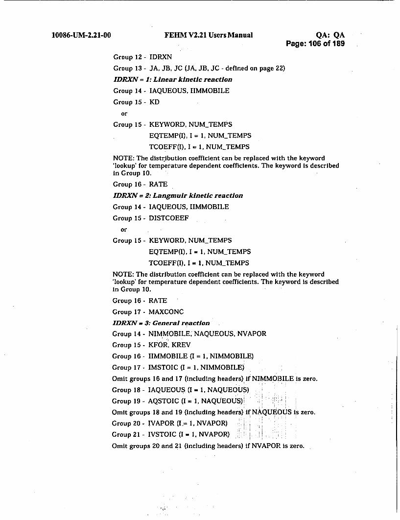
10086-UM-2.21-00 FEHM V2.21 Users Manual QA: QAPage: 106 of 189
Group 12 - IDRXN
Group 13 - JA, JB, JC (JA, JB, JC - defined on page 22)
IDRXN = 1: Linear kinetic reaction
Group 14 - IAQUEOUS, IIMMOBILE
Group 15 - KD
or
Group 15 - KEYWORD, NUM_TEMPS
EQTEMP(I), I = 1, NUM_TEMPS
TCOEFF(I), I = 1, NUMTEMPS
NOTE: The distribution coefficient can be replaced with the keyword'lookup' for temperature dependent coefficients. The keyword is describedin Group 10.
Group 16- RATE
IDRXN = 2: Langmuir kinetic reaction
Group 14 - IAQUEOUS, IMMOBILE
Group 15- DISTCOEEF
or
Group 15 - KEYWORD, NUM_TEMPS
EQTEMP(I), I = 1, NUMTEMPS
TCOEFF(I), I 1, NUMTEMPS
NOTE: The distribution coefficient can be replaced with the keyword'lookup' for temperature dependent coefficients. The keyword is describedin Group 10.
Group 16- RATE
Group 17 - MAXCONC
IDRXN = 3: General reaction
Group 14 - NIMMOBILE, NAQUEOUS, NVAPOR
Group 15 - KFOR, KREV
Group 16 - IIMMOBILE (I = 1, NIMMOBILE)
Group 17 - IMSTOIC (I = 1, NIMMOBILE)
Omit groups 16 and 17 (including headers) if NIMMOBILE is zero.
Group 18 - IAQUEOUS (I = 1, NAQUEOUS)
Group 19 - AQSTOIC (I = 1, NAQUEOUS)
Omit groups 18 and 19 (including headers) if NAQUEOUS is zero.
Group 20 - IVAPOR (I.= 1, NVAPOR)
Group 21 - IVSTOIC (I = 1, NVAPOR)
Omit groups 20 and 21 (including headers) if NVAPOR is zero.

10086-UM-2.21-00 FERM V2.21 Users Manual QA: QAPage: 107 of 189
IDRXN = 4: Dual Monod kinetics biodegradation reaction
Group 14 - NAQUEOUS (must be >2 and < 5), NIMMOBILE
Group 15 - SUBSTRATE, ELECACC, COMP3, COMP4, COMP5
Note that the users choice of NAQUEOUS determines whether COMP3,COMP4, and COMP5 need to be entered. NIMMOBILE must be 1.NAQUEOUS also determines whether the COMP3, COMP4, and COMP5stoichiometries are to be used by the code. However values must always beentered for groups 21-23 regardless of the value of NAQUEOUS.
Group 16 - BIOMASS
Group 17 - KS
Group 18 - KA
Group 19- DECAY
Group 20 - ELECACCSTOIC
Group 21 - COMP3STOIC
Group 22 - COMP4STOIC
Group 23 - COMP5STOIC
Group 24 - PHTHRESH
Group 25 - QM
Group 26 - YIELD
Group 27 - XMINIT
Group 28 - NBIOFRM
Omit Group 29 if NBIOFRM = 0
Group 29 - ICBIO (I = 1, NBIOFRM)
IDRXN=5': Radioactive Decay Reaction
Group 14 - HALFLIFE
Group 15- RXNTYPE
Group 16 - PARENT, DAUGHTER
IDRXN=6: Kinetic Henry's Law reaction
Group 14 - IAQUEOUS, IVAPOR
Group 15 - KH
Group 16- RATE
IDRXN = 7: Kinetic precipitation/dissolution reaction for totalcomponent concentrations
Group 14 - IIMMOBILE
Group 15- NAQUEOUS
Group 16 - IAQUEOUS (I = 1, NAQUEOUS)
Group 17 - IMSTOIC
Group 18 - AQSTOIC (I = 1, NAQUEOUS)

10086-UM-2.21-00 FEHM V2.21 Users Manual QA: QAPage: 108 of 189
Group 19- SOLUBILITY
or
Group 19 - KEYWORD, NUMTEMPS
EQTEMP(I), I 1 1, NUMTEMPS
TCOEFF(I), I = 1, NUMTEMPS
NOTE: Solubility can be replaced with the keyword 'lookup' fortemperature dependent solubilities. The keyword is described in Group 10.
Group 20 - RATE
Group 21 - SAREA
IDRXN = 8: Kinetic precipitation/dissolution reaction for totalcomponent concentrations with rates based on free-ionconcentrations
NOTE: The input is identical to that for reaction model 7.
Input Variable Format Description
NCPLX integer Number of aqueous complexes (equal to number of equilibrium
reactions)
NUMRXN integer Number of kinetic reactions
NGROUPS integer Number of groups. See GROUP to determine how to set thisparameter.
GROUP integer This variable controls the selective coupling solution methodemployed by FEHM. NCPNT values are entered for each line ofinput, and NGROUPS lines of input are required, one for eachgroup. If a value is non-zero, then that aqueous component ispresent in the group. A value of zero denotes that the species isnot present in the group. Grouping of aqueous components thattare part in rapid kinetic reactions is required for convergence.However, memory requirements increase as the square of themaximum number of aqueous components in a group.
IDCPNT integer For each total aqueous component, the number identifying eachtotal aqueous component (e.g. 1, 2, etc.)
CPNTNAM character For each total aqueous component, the name of the total aqueouscomponent (e.g. Sulfate)
IFXCONC integer For each total aqueous component, the Flag denoting the type oftotal aqueous component
1 - total aqueous concentration is specified in TRAC macro2 - specify log of free ion concentration in TRAC macro (use for
pH). For example, if H+ is the component, IFXCONC of 2allows for pH to be directly input in place of concentrationvalues In the TRAC macro.

10086-UM-2.21-00 FEIM V2.21 Users Manual QA: QAPage: 109 of 189
Input Variable Format Description
CPNTPRT integer For each total aqueous component, the Flag denoting which totalaqueous component concentrations are printed to the ".trc" file andthe AVS files.
0 - Print to file1 - Do not print to file
CPNTGS real Guess for the initial uncomplexed component concentration usedin speciation reactions. We recommend 1.0e.-9. On rare occasions,the chemical speciation solver may have trouble converging.Choosing more representative values for CPNTGS will helpconvergence.
IDCPLX integer For each aqueous complex, the number identifying each aqueouscomplex. By convention, the first complex should be given thenumber 101, the second, 102, etc.
CPLXNAM character For each aqueous complex, the name of the aqueous complex(e.g. H2SO 4 )
CPLXPRT integer For each aqueous complex, the Flag denoting which aqueouscomplex concentrations are printed to the "trc" file and the AVSfiles.
0 - Print to file1 - Do'not print to file
IDIMM integer For each immobile component, the number identifying eachimmobile component (e.g. 1, 2, etc.)
IMMNAM character For each immobile component, the name of the immobilecomponent (e.g. Calcite, Co[adsorbed])
IMMPRT integer For each immobile component, the Flag denoting which immobilecomponent concentrations are printed to the "trc" file and the AVSfiles.
0 - Print to file1 - Do not print to file
IDVAP integer Fore each vapor component, the number identifying each vaporcomponent (e.g. 1, 2, etc.)
VAPNAM character For each vapor component, the name of the vapor component (e.g.C02[gas])
VAPPRT integer For each vapor component, the Flag denoting which vaporcomponent concentrations are printed to the ".trc" file and the AVSfiles.
0 - Print to file1 -Do not print to file -
ISKIP integer Flag denoting whether chemical speciation calculations should bedone at nodes which have already converged in a previoustransport iteration
0 - Do chemical speciation calculationS at each node for everyiteration (recommended option)

ir
10086-UM-2.21-00 FEHM V2.21 Users Manual QA: QAPage: 110 of 189
Input Variable Format Description
1 -To save computational time, this options tells FEHM to doequilibrium speciation calculations only at nodes which havenot converged during the previous transport iteration.Sometimes, this option can lead to mass balance errors(mass balances can be checked in the ".out" file to see ifresults are satisfactory). This option is only recommended forvery large problems.
RSDMAX real The tolerance for the equilibrium speciation calculations. Werecommend lx1i0- for most problems.
HEADING character One line descriptive comment which precedes the LOGKEQheading
LOGKEQ integer Flag denoting the whether K or log K is entered by the user'- constants are given as K1 - constants are given as log K
CKEQ real For each aqueous complex, the equilibrium constant
HEQ real For each aqueous complex, the enthalpy of the equilibriumreaction. The Van Hoff equation is used to determine the value ofthe equilibrium constant as a function of temperature. Note thekeyword 'lookup' (see page 105) can be used in the place of CKEQand HEQ.
KEYWORD character Keyword 'lookup' designating a lookup table will be used todescribe the equilibrium constant as function of temperature.
NUMTEMPS integer Number of values of temperature and K that will be used todescribe K as a function of temperature.
EQTEMP real Temperatures for K function (°C)
LKEQ real Equilibrium constants for K function
STOIC real For each aqueous complex, the stoichiometry describing how to"make" the complex from the total aqueous components must beentered. If positive, the solute is a reactant; if negative, the solute isa product; and if 0, the solute is not present in the reaction.
IDRXN integer Fo4 each kinetic reaction, this parameter specifies kinetic reactionmodel. Currently, the following reaction models are available.Additional kinetic formulations can be added without significantcode development.
1 - linear kinetic reaction2 - langmuir kinetic reaction3 - general kinetic reaction4 - dual Monod biodegradation reaction5 - radioactive decay reaction6 - kinetic Henry's law reaction7 - precipitation/dissolution reaction8 - precipitation/dissolution reaction with rates based on free-ion
concentration

10086-UM-2.21-OO FETM V2.21 Users Manual QA: QAPage: 111 of 189
Input Variable Format Description
JA, JB, JC integer JA, JB, JC are described on page 22. Here these parameters areused to specify the nodes at which the current kinetic reactiontakes place. If the reaction takes place throughout the problemdomain simply enter 1 0 0.
IDRXN = 1: Linear Kinetic Reaction
IAQUEOUS
IIMMOBILE
KD
KEYWORD
NUMTEMPS
integer
integer
real
character
integer
The aqueous component number (e.g. 1, 2, etc.) or the aqueouscomplex number (e.g. 101, 102, etc.) which corresponds to thesorbing component
The immobile component number (e.g. 1, 2, etc.) whichcorresponds to the sorbed component
Distribution coefficient (kg water / kg rock)
Keyword 'lookup' designating a lookup table will be used todescribe the distribution coefficient as a function of temperature.
Number of values (temperatures and distribution coefficients) thatwill be used to describe KD as a function of temperature.
EQTEMP real Temperatures for distribution coefficient function (0C)
TCOEFF real Distribution coefficients corresponding to temperatures.
RATE real Reaction rate parameter (1/hr)
IDRXN = 2: Langmuir Kinetic Reaction
IAQUEOUS integer The aqueous component number (e.g. 1, 2, etc.) or the aqueouscomplex number (e.g. 101,102, etc.) which corresponds to thesorbing component
IIMMOBILE integer The immobile component number (e.g. 1, 2, etc.) whichcorresponds to the sorbed component
DISTCOEFF real Distribution coefficient (kg water/ moles)
KEYWORD character Keyword 'lookup' designating a lookup table will be used todescribe the distribution coefficient as a function of temperature.
NUM_TEMPS integer Number of values (temperatures and distribution coefficients) thatwill be used to describe DISTCOEFF as a function of temperature.
EQTEMP real Temperatures for distribution coefficient function (°C)
TCOEFF real Distribution coefficients for DISTCOEFF as a function oftemperature.
RATE real Reaction rate parameter (1/hr)
MAXCONC real Maximum concentration (moles/kg rock)
IDRXN = 3: General Kinetic Reaction
NIMMOBILE integer The number of immobile components which participate in thereaction
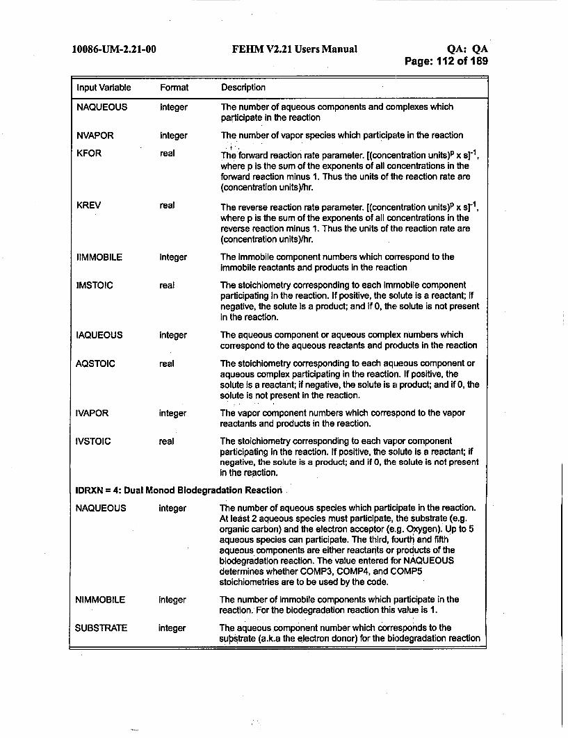
10086-UM-2.21-OO FEHM V2.21 Users Manual QA: QAPage: 112 of 189
Input Variable Format Description
NAQUEOUS integer
integer
real
NVAPOR
KFOR
KREV real
IIMMOBILE
IMSTOIC
IAQUEOUS
AQSTOIC
IVAPOR
IVSTOIC
integer
real
integer
real
integer
real
The number of aqueous components and complexes whichparticipate in the reaction
The number of vapor species which participate in the reaction
The forward reaction rate parameter. [(concentration units)P x s]"1,where p is the sum of the exponents of all concentrations in theforward reaction minus 1. Thus the units of the reaction rate are(concentration units)/hr.
The reverse reaction rate parameter. [(concentration units)P x s]- 1,where p is the sum of the exponents of all concentrations in thereverse reaction minus 1. Thus the units of the reaction rate are(concentration units)/hr.
The immobile component numbers which correspond to theImmobile reactants and products in the reaction
The stoichiometry corresponding to each immobile componentparticipating in the reaction. If positive, the solute is a reactant; ifnegative, the solute is a product; and if 0, the solute is not presentin the reaction.
The aqueous component or aqueous complex numbers whichcorrespond to the aqueous reactants and products in the reaction
The stoichiometry corresponding to each aqueous component oraqueous complex participating in the reaction. If positive, thesolute is a reactant; if negative, the solute is a product; and if 0, thesolute is not present in the reaction.
The vapor component numbers which correspond to the vaporreactants and products in the reaction.
The stoichiometry corresponding to each vapor componentparticipating in the reaction. If positive, the solute is a reactant; ifnegative, the solute is a product; and if 0, the solute is not presentin the reaction.
IDRXN = 4: Dual Monod Biodegradation Reaction
NAQUEOUS
NIMMOBILE
SUBSTRATE
integer
integer
integer
The number of aqueous species which participate in the reaction.At least 2 aqueous species must participate, the substrate (e.g.organic carbon) and the electron acceptor (e.g. Oxygen). Up to 5aqueous species can participate. The third, fourth and fifthaqueous components are either reactants or products of thebiodegradation reaction. The value entered for NAQUEOUSdetermines whether COMP3, COMP4, and COMP5stoichiometries are to be used by the code.
The number of immobile components which participate in thereaction. For the biodegradation reaction this value is 1.
The aqueous component number which corresponds to thesupstrate (a.k.a the electron donor) for the biodegradation reaction

10086-UM-2.21-00 FEHM V2.21 Users Manual QA: QAPage: 113 of 189
Input Variable Format Description
ELECACC integer The aqueous component number which corresponds to theelectron acceptor for the biodegradation reaction
COMP3 integer The aqueous component number which corresponds to a reactant
or product in the biodegradation reaction (e.g. C02, NH 3 , H*, etc.).Note that this parameter is optional. COMP3 should only beentered if NAQUEOUS>2.
COMP4 integer The aqueous component number which corresponds to a reactant
or product in the biodegradation reaction (e.g. C02, NH 3 , H+,etc.).Note that this parameter is optional. COMP4 should only beentered if NAQUEOUS>3.
COMP5 integer The aqueous component number which corresponds to a reactantorproduct in the biodegradation reaction (e.g. C02, NH 3, H+,etc.)Note that this parameter is optional. COMP5 should only beentered if NAQUEOUS>4.
BIOMASS real The solid component number which corresponds to the biomass(this is the immobile component).
KS real The Monod half-maximum-rate concentration for the substrate(moles/ kg water)
KA real The Monod half-maximum-rate concentration for the electronacceptor (moles/ kg water)
DECAY real First order microbial decay coefficient (hr')
ELECACCSTOIC
COMP3STOIC
COMP4STOIC
COMP5STOIC
PHTHRESH
QM
real
real
real
real
real
real
The stoichiometry corresponding to the electron acceptor. Notethat the stoichiometry of the substrate is I by definition.
The stoichiometry corresponding to COMP3. A value is alwaysentered whether or not it is used.
The stoichiometry corresponding to COMP4. A value is alwaysentered whether or not it is used.
The stoichiometry corresponding to COMP5. A value is alwaysentered whether or not it is used.
In many systems, the biodegradation reaction will stop as the pHbecomes either too acidic or basic. This parameter can be used tostop the biodegradation reaction once the simulated pHapproaches a certain value. For example, if PHTHRESH = 10, thebiodegradation reaction will cease if the pH is above 10 in thesimulation. Note that PHTHRESH is an upper threshold for pH.
The maximum specific rate of substrate utilization (moles/kg
biomass/hr)
The microbial yield coefficient (kg biomass/mole substrate)YIELD real

10086-UM-2.21-00 FEHM V2.21 Users Manual QA: QAPage: 114 of 189
Input Variable Format Description
XMINIT real In many systems, biomass does not decay below a certainconcentration. The biomass concentration is not allowed to fallbelow XMINIT (moles/ kg rock).
NBIOFRM integer Depending on the problem setup, many aqueous complexes canbe formed from a total aqueous component. Only some of thesecomplexes may be biodegradable. This parameter is used tospecify which forms (the total aqueous concentration, the free ionconcentration, or various complex concentrations) of thecomponent degrade. If NBIOFRM = 0, the total aqueousconcentration of the component will degrade and the nextparameter ICBIO should be omitted.lf NBIOFRM = 2, then twoforms of this component degrade. These forms are specified usingIBIO.
ICBIO integer Specify the aqueous component numbers (e.g. 1) or aqueouscomplex numbers (e.g. 101,102, etc.) corresponding to thebiodegradable form of the substrate.
IDRXN = 5: Radioactive Decay Reaction
HALFLIFE real Half life (years)
RXNTYPE integer Flag denoting the type of component participating in the reaction:0 - Solid1 - Liquid
-A -Vapor
PARENT integer The number of the component which corresponds to the parent inthe radioactive decay reaction
DAUGHTER integer The number of the component which corresponds to the daughterin the radioactive decay reaction. If the simulation does not modelthe daughter product set daughter = 0.
IDRXN = 7: Kinetic PrecipitationlDissolution Reaction
IIMMOBILE integer The immobile component number (e.g. 1, 2, etc.) whichcorresponds to the dissolving mineral
NAQUEOUS integer The number of aqueous species which participate in the reaction
IAQUEOUS integer The aqueous component numbers which correspond to theaqueous components which enter into the solubility productexpression. Note that the total aqueous concentration of thecomponent will dissolve.
IMSTOIC real The stoichiometry corresponding to the immobile componentparticipating in the reaction. If positive, the solute is a reactant; ifnegative, the solute is a product; and if 0, the solute is not presentin the reaction.

10086-UM-2.21-00 FEHM V2.21 Users Manual QA: QAPage: 115 of 189
Input Variable Format Description
AQSTOIC real The stoichiometry corresponding to the aqueous componentsparticipating in the reaction. If positive, the solute is a reactant; ifnegative, the solute is a product; and if 0, the solute is not presentin the reaction.
SOLUBILITY real The solubility product. The units of the solubiFity product depend onthe number of aqueous components participating in the reaction.For example, if there are two aqueous components participatingthe units would be (moles 2/[kg water] 2)
KEYWORD character Keyword 'lookup' designating a lookup table will be used todescribe the solubility as a function of temperature.
NUMTEMPS integer Number of values of temperature and solubility that will be used todescribe solubility as a function of temperature.
EQTEMP real Temperatures for solubility function (°C)
TCOEFF real Solubilities for solubility as a function of temperature.
RATE real Reaction rate parameter (moles/[m2s])
SAREA real Surface area of the mineral (m2/m3 rock)
IDRXN = 8: Kinetic PrecipitationlDissolution Reaction (rates based on free-ion concentrations)This model and its input are the same as for IDRXN = 7 except that the rates are based on the free-ionconcentration instead of the total concentration.
In general, the following examples illustrate only portions of the rxn macroand putting all of these example inputs together will not result in aworking FEHM rxn macro. However, the dissolution example (the lastexample in this section) provides an example of a complete rxn macro andcorresponds to the first example given for the trac macro (page 140). Inaddition, the *Reactive Transport Example" (Section 9.5) and theValidation Test Plan for the FEHM Application Version 2.21(10086-VTP-2.21-00) include full example problems with input files whichdemonstrate the use of rxn. These input files can be used to see how rxnfits in with the other macros. Specifically, the information in rxn must beconsistent with the trac macro. For example, if a linear kinetic sorptionreaction is invoked by rxn, a liquid component and solid component mustbe specified in the trac macro.
General Reaction Parameters. In the following example two aqueouscomplexes and four kinetic reactions are specified. Three liquidcomponents, Co, Fe, and EDTA, two complexes, CoEDTA and FeEDTA, andthree immobile species, Co, CoEDTA and FeEDTA, are identified. Aqueouscomponents 1 and 3 are coupled during solution while 2 is solvedindependently. Note that group 6 data has been omitted since there are novapor species in this example.
Equilibrium Reaction Parameters. Equilibrium speciation reactionsmodeled by FEHM can be written in the following general form:

10086-UM-2.21-flO FEHM V2.21 Users Manual QA: QAPage: 116 of 189
N,
a, aje~j<= I,..., Nx1=I •
(1)
where Cj is the chemical formula for the aqueous component J, and 1i is
the chemical formula for the aqueous complex i, aij is a stoichiometriccoefficient (STOIC) giving the number of moles of component j in complex
i, Nx is the number of aqueous complexes, and kc is the number ofaqueous components. Here is a simple example of an equilibrium speciationreaction.
aA + bB* AaBb (2)
where a and b are the stoichiometric coefficients of components A and B,
respectively. At equilibrium, the concentrations of A, B, and AaBb must
satisfy the law of mass action for this reaction:
K [AaBb][A] a[B]b
(3)
where K is the equilibrium constant (CKEQ) for the reaction and [X] is themolar concentration of species X. The total aqueous concentrations ofcomponents A and B are given by:
UA = [A]+a[AaBb]
Ub = [B] + b[AaBb]
(4)
(5)

10086-UM-2.21-00 FEIM V2.21 Users Manual QA: QAPage: 117 of 189
Therefore, the total aqueous concentrations, U, are functions of theuncomplexed component concentrations and the complex concentrations.Note that the kinetic reactions discussed in the next section are functionsof the uncomplexed component concentrations and complex concentrationswith the exception of the radioactive decay and precipitation/dissolutionreaction in which the total aqueous concentration is used in the reactionrate law.
The following input describes the equilibrium speciation relations betweenthe total aqueous components and aqueous complexes. Recall that thenames of the components and aqueous complexes are given in Groups 3-6.The skip node option, ISKIP, is turned off and the tolerance for thespeciation solver, !RSDMAX, is set to le-9 which is the recommended value.The stoichiometry, STOIC, is specified so that the components Co andEDTA make up the first complex CoEDTA, and the components Fe andEDTA make up the second complex FeEDTA. The equilibrium constants,CKEQ, for CoEDTA and FeEDTA are l.e18 and 6.31e27, respectively. Theenthalpy change is 0.
** ISKIP ** Group 70**RSDMAX ** Group 81 e-9** Chemical Information **
**LOGKEQ ** Group 90** CKEQ HEQ * Group 101.0e18 06.31e27 0** STOIC ** Group 111.0 0.0 1.00.0 1.0 1.0
Below is an example of using the 'lookup' keyword in place of CKEQ andHEQ. This example describes the temperature dependence of the
equilibrium constant of complex HC0 3 ". Note that LOGKEQ = 1 in thisexample, so log K is specified in the input rather than K.
** LOGKEQ ** Group 91** KEYWORD NUMTEMPS Group 10lookup 6
0 25 60 100 150 200-6.58 -6.3447 -6.2684 -6.3882 -6.7235 -7.24
General Kinetic Parameters. In FEHM, eight kinetic reaction modelsare supported. Additional kinetic subroutines can be added withoutsignificant code development. The following is an example of input for thegeneral kinetic parameters. A linear kinetic reaction, IDRXN = 1, isspecified as occurring at each node in the problem (JA = 1, JB and JC = 0).
IDRXN = 1: Linear Kinetic Reaction. The retardation of contaminants dueto adsorption/desorption can be modeled with a linear kinetic sorption/
I

I
10086-UM-2.21-00 FEHIM V2.21 Users Manual QA: QAPage: 118 of 189
*IDRXN Group 12
*JA JB JC Group 131 0 0
desorption expression. The rate of adsorption/desorption of componentj isgiven by:
Rj = m-.(j ' (6)
where c1 denotes the uncomplexed aqueous concentration ofj
(IAQUEOUS), m1 denotes the adsorbed concentration of speciesj
{IIMMOBILE),km is the mass transfer coefficient (RATE), and KD is the
distribution coefficient (KD). As km -- oo, this expression reduces to the
linear equilibrium isotherm. The following example illustrates input for alinear kinetic reaction. In this kinetic reaction, aqueous component 1
adsorbs to form the immobile component 3. The KD for the reaction is 5.07
and the mass transfer coefficient is 1.0.
** IDRXN ** Group 121**JA JB JC** Group 13
1 0 0** IAQ IMMOBILE ** Group 141 3** KD ** Group 155.07** RATE Group 161.0
IDRXN = 2: Langmuir Kinetic Reaction. The Langmuir kinetic reactionrate law is given by:
Rj = -kkm2(KL(mJ MAX (7)
where km is the rate constant for desorption (RATE), p is the bulk rock
density {DENR), 0 is the porosity (POR). KL is the distribution
MAXcoefficient (DISTCOEFF), and m- is the maxirnu in concentration that
can adsorb onto the solid (MAXCONC]. As km --4 Q0 this expression-
reduces to the Langmuir equilibrium isotherm. Exa iple Input for aLangmuir kinetic reaction follows. In this kinetic re :tion, aqueouscomplex 101 sorbs to form immobile component 1. Te distributioncoefficient for the reaction is 2.e5 and the mass transfer coefficient is 0.05.The maximum sorbed concentration is 1.69e-5.

10086-UM-2.21-00 FERM V2.21 Users Manual QA: QAPage: 119 of 189
** IDRXN ** Group 12
2**JA JB JC** Group 131 0 0** IAQ IMMOBILE ** Group 14101 1** DISTCO ** Group 152.0e5
RATE ** Group 160.05** MAXCO ** Group 171.69e-5
IDRXN = 3: General Kinetic Reaction. Many reactions fall under thecategory of the general kinetic reaction. The reaction is described by aforward rate constant {KFOR), a reverse rate constant {KREV), and a setof stoichiometric coefficients. The form of the general reversible reaction isgiven by:
N, + N. + N, + NV
j=1jjj 4*
N, + N + Nm +N
k=I"1k'k (8)
where N, is the number of aqueous components, Nx is the number of
aqueous complexes {NAQUEOUS= Nc+Nx},Nm is the number of immobile
components (NIMMOBILE), Nv is the number of vapor components
{NVAPOR), 11j are reactant stoichiometric coefficients, lk' are product
stoichiometric coefficients, and 1i is the chemical formula for species i,
which may be an uncomplexed aqueous component, aqueous complex,immobile component or vapor component. The rate law for a generalreversible reaction is given by the following expression:
R(z,) = (fi....T1I)[kfN z71 - ,,+k +N,+N,
S= I k=I
(9)
where zi is the concentration of species i. The following is example input
for a general kinetic reaction. Solid component 1 reacts to form solidcomponents 2 and 3. The forward reaction rate is 1.26e-2 and the reversereaction rate is 0. Therefore, this is an irreversible reaction. Note also thatonly solid components are reacting so groups 18-21 have been omitted.

10086-UM-2.21-00 FEHM V2.21 Users Manual QA: QAPage: 120 of 189
** IDRXN ** Group 123** JA JB JC* Group 13
1 0 0** NIMM NAQSP NVAPOR ** Group 143 0 0** KFOR KREV ** Group 151.26e-2 0.0** I1MM ** Group 161 2 3** IMSTOIC ** Group 171.0 -1.0 -1.0
IDRXN =4: Dual Monod Biodegradation Reaction. Biodegradation is anirreversible process in which bacteria oxidize an organic substrate toproduce energy and biomass. In addition to biomass, the biodegradationprocess requires the presence of an electron acceptor (e.g. oxygen, nitrate,etc.) and nutrients (e.g. nitrogen and phosphorous). An example of abiodegradation reaction is given by the following reaction:
Substrate + Electron Acceptor + H+ + Nutrients -> cells + CO 2 + H2 0 + NH 3
FEHM models the rate of biodegradation of a substrate with amultiplicative Monod model, which is given by:
R [S] [A] (10)s -qmmbT" + [S]KA + [A]
where [S] is the aqueous concentration of substrate (a.k.a the electrondonor) (SUBSTRATE), [A] is the aqueous concentration of the electronacceptor {ELECACC), and mb is the concentration of the immobile biomass(BIOMASS). The parameter qm is the maximum specific rate of substrateutilization (QM), which represents the maximum amount of substrate thatcan be consumed per unit mass of bacteria per unit time. The parametersKS (KS) and KA {KA) are the Monod half-maximum-rate concentrations forthe electron donor and electron acceptor, respectively. The rate of microbialgrowth is given by the synthesis rate (which is proportional to the rate ofsubstrate degradation) minus a first-order decay rate.
Rcells , YRS- b(mb - mb, nit) (11)
where Y is the microbial yield coefficient (YIELD) and b is the first-ordermicrobial decay coefficient (DECAY). In the above equation, theassumption is made that the background conditions are sufficient tosustain a microbial population of a given size; therefore, the biomassconcentration is not allowed to fall below its initial backgroundconcentration (mb, nit) {XMINIT). In the following example of input for adual monod biodegradation reaction, aqueous component 3 is the substrateand aqueous component 4 is the electron acceptor. Note that there are onlytwo entries in Group 15 and Groups 21-23 are omitted since NAQUEOUS =
2. In addition Group 29 data is left out since NBIOFRM = 0.

10086-UM-2.21-00 FEHM V2.21 Users Manual QA: QAPage: 121 of 189
** IDRXN ** Group 124** JA JB JC0* Group 13
1 0 0** NAQSP NIMMOBILE ** Group 14
2 1**SUBSTRA ELECACC** Group 15
3 4** BIOMASS ** Group 164** KS ** Group 170.201 e-3** KA ** Group 180.00625e-3** DECAY ** Group 190.0020833** EASTOIC ** Group 203.10345** COMP3STOIC ** Group 210** COMP4STOIC ** Group 220** COMP5STOIC ** Group 230** PHTHRSH ** Group 248** QM Group 258.0226 e-4** YIELD 0* Group 2644.8732** XMINIT Group 270.0** NBIOFRM ** Group 280*0 ICBIO** Group 29
IDRXN = 5: Radioactive Decay Reaction. Radioactive decay is a simplefirst order decay process given by:
A-4B (12)
where A is the parent (PARENT) and B is the daughter product(DAUGHTER). The half life of the reaction is defined as the time it takesfor the concentration of A to decrease by a factor of 2. In the followingexample of input for a radioactive decay reaction, aqueous component 2,the parent, reacts to form aqueous component 3, the daughter product. Thehalf life for the reaction is 432.0 years.

10086-UM-2.21-00 FEHM V2.21 Users Manual QA: QAPage: 122 of 189
** IDRXN ** Group 125**JA JB JC Group 13
1 0 0** HALFLIFE ** Group 14432.0** RXNTYPE ** Group 151** PARENT DAUGHTER ** Group 162 3
IDRXN = 7: Kinetic Precipitation/Dissolution Reaction. A generalreaction describing the precipitation/dissolution of a mineral p(IIMMOBILE} can be written in the following form:
mPI € * 9PICl + IpIC2 + ... + 1IPCN (13)
where the ci are the aqueous concentrations (IAQUEOUS) and the tpi
are stoichiometric coefficients (AQSTOIC). The equilibrium constant forthis reaction is known as the solubility product. Since the activity of a pure
solid Is equal to one, the reaction quotient Qp Is defined as follows:
N,QP = Jc (14)
J=1
At equilibrium, Qp Is equal to the solubility product. The surface-controlled rate of precipitation/dissolution of a mineral is given by:
R(mp) = sign logLj)A kp ~ -1J (15)Qp sp
where Ap is reactive surface area of the mineral (AREA), kp is the
precipitation rate constant (RATE), and Ksp is the solubility product
(SOLUBILITY). Currently, this precipitation/dissolution subroutine onlyallows for the total aqueous concentration of a component to dissolve. Thedissolution of uncomplexed aqueous concentration and complexconcentrations is not currently supported.
The following is example input for a kinetic precipitation/dissolutionreaction (calcite dissolution). This example corresponds to the exampleused for the trac macro (page 140). A single kinetic reaction is specifiedwith no aqueous complexes. The liquid and immobile components areidentified. Aqueous component I participates in the precipitation/dissolution reaction with immobile component 1. No data is input forgroups 4, 6, 9, 10, and 11. The solubility product for the reaction is 6.26e-5and the reaction rate constant is 100.

10086-UM-2.21-OO FEHM V2.21 Users Manual QA: QAPage: 123 of 189
rxn** NCPLX
0** GROUP*11
** IDCPNT1
** IDCPLX** IDIMM1
** IDVAP** ISKIP **
0**RSDMAXle-13** Chemical** LOGKEQ** CKEQ** STOIC **
** IDRXN **
7** JA
** IIMMOBLE1
NUMRXN **1
CPNTNAMCa[aq]CPLXNAMIMMNAMCa[s]VAPNAM
IFXCONC0CPLXPRTIMMPRT **
0VAPPRT
CPNTPRT0**
CPNTGS1.0e-9
**
**
reaction
HEQ0*
information **
Group 1
Group 2
Group 3
Group 4Group 5
Group 6Group 7
Group 8
Group 9Group 10Group 11Group 12
Group 13
Group 14
Group 15
Group 16
Group 17
Group 18
Group 19
Group 20
Group 21
JB0**t
JC **
0
** NAQSP **14
** IAQ **1
** IMSTOIC1
** AQSTOIC
** SOLPROD6.26e-5** RATE **100** AREA **1.0
**
**•
IDRXN = 8: Kinetic Precipitation/Dissolution Reaction (rates based onfree-ion concentrations). The reaction model'ed is !analogous to that forIDRXN =7, except that rates are based on the u co: plexed (free-ton)concentration of the species. The total concentrattIon s equal to the free ionconcentration + all of the complex concentrations, For a more detaileddiscussion of the differences between total aque us and free-ionconcentration, see the "Models and Methods aSu y of the FEHMApplication [Zyvoloski et al. 1999, page 39ý Equatýon (79)]. For example, fora species such as Cobalt from the multisolute problemn (see Section 9.5,"Reactive Transport Example," on page 182),1 th. free Ion concentration issimply the concentration of Cobalt in it's uncomplexed state. The totalCobalt would be Free Ion Cobalt + all Cobalt Complexes (e.g. CoEDTA from

10086-UM-2.21-00 FEHM V2.21 Users Manual QA: QAPage: 124 of 189
the multisolute verification problem). Using IDRXN = 7 allows the totalCobalt to dissolve, while IDRXN= 8 allows only the free ion Cobalt todissolve.
6.2.60 Control statement sol (optional)
Group 1 - NTT,INTG
Input Variable Format Default Description
NTT integer 1 Parameter that defines the type of solution requiredNTT > 0 coupled solutionN'- < 0 heat transfer only solution
INTG integer -1 Parameter that defines element integration typeINTG < 0 Lobatto (node point) quadrature is used,
recommended for heat and mass problems without stress.INTG > 0 Gauss quadrature is used, recommended for
problems requiring a stress solution.
The following is an example of sol. In this example, a coupled heat-masssolution using Lobatto quadrature is specified.
Sol
6.2.61 Control statement sptr (optional)
Streamline particle tracking is invoked with this control statement.
Group 1 - DTMX, IPRT, IPRTO, RSEED
Optional keyword "tcurve" is input to indicate that transfer function curvesshould be input to model matrix diffusion. It is followed by NUMPARAMS
and TFILENAME.
KEYWORD
NUMPARAMS
TFILENAME
Optional keywords "po", "sa", "pe", *de", "pr", "te", "zo" define parameters tobe output.
KEYWORD
Group 2- COURANTFACTOR, IPRTR, ITENSOR, IREVERS,FREEZ_TIME
Group 3 - KEYWORD
The Group 3 keyword (tprp') specifies that transport properties will beentered on subsequent lines. The transport properties it1put (Group 4)depend on the value of TPRPFLAG, the first value input for that group.For TPRPFLAG = 2 or 4, format of Group 4 input also' depends on the formof the dispersion coefficient tensor, as selected using' the flag ITENSOR(Group 2).

10086-UM-2.21-00 FEHM V2.21 Users Manual QA: QAPage: 125 of 189
TPRP FLAG =1:
Group 4 - TPRP_FLAG, KD
TPRPFLAG = :
ITENSOR = 1
Group 4 - TPRPFLAG, KD, DM, AI, A2, A3, A4, ASX, ASY, VRATIO
ITENSOR = 2
Group 4 - TPRPFLAG, KD, DM, AL, ATH, ATV, VRATIO
ITENSOR = 3
Group 4 - TPRPFLAG, KD, DM, ALH, ALV, ATH, ATV, VRATIO
ITENSOR = 4
Group 4 - TPRPFLAG, KD, DM, AL, AT, VRATIO
ITENSOR = 5
Group 4 - TPRPFLAG, KD, AL, ATH, ATV, DM, VRATIO
TPRP_ FLAG = 3:
Group 4 - TPRPFLAG, KD, DIFM, RDFRAC, POR._MATRIX,APERTURE
TPRPFLAG = 4:
ITENSOR = 1
Group 4 - TPRPFLAG, KD, DIFM, RDFRAC, POR.MATRIX,APERTURE, DM, Al, A2, A3, A4, ASX, ASY, VRATIO
ITENSOR = 2
Group 4 - TPRPFLAG, KD, DIFM, RDFRAC, POR.MATRIX,APERTURE, DM, AL, ATH, ATV, VRATIO
ITENSOR = 3
Group 4 - TPRPFLAG, KD, DIFM, RDFRAC, POR..MATRIX,APERTURE, DM, ALH, ALV, ATH, ATV, VRATIO
ITENSOR = 4
Group 4 - TPRPFLAG, KD, DIFM, RDFRAC, PORMATRIX,APERTURE, DM, AL, AT, VRATIO
ITENSOR = 5 (not recommended, included for compatibility with olderversions of the code)
Group 4 - TPRPFLAG, KD, DIFM, RDFRAC, POR_.MATRIX,APERTURE, AL, ATH, ATV, DM, VRATIO
Group 5 - JA, JB, JC, MODELNUMBER
Group 4 is ended when a blank line is encountered. The MODELNUMBERis incremented each time a Group 4 line is read, and Group 5 lines refer tothis parameter.
The optional keyword 'zbtc' indicates that breakthrough curves will becomputed for specified zones. It is followed by NZBTC and ZBTC.

10086-UM-2.21-OO FEHM V2.21 Users Manual QA: QAPage: 126 of 189
KEYWORD
NZBTC
ZBTC
Group 6 - ITM, IST
Group 7 - NX, NY, NZ
Group 8 - X1O, Y10, Z10
Group 9 - XDIM, YDIM, ZDIM
Group 10 - IJKV(I), XI(I), Y1(I), ZI(I) for I I 1 to NUMPART
Group 10 input is terminated with a blank line.
Note when IST = 0 or 1, Group 10 is used and place holders are inserted forGroups 7-9; however, when IST = 2, Group 10 is not implemented andGroups 7-9 are used.
Input Variable Format Description
DTMX real Time step control (seconds). FEHM will account for all particlesevery abs(dtmx) seconds and write information to the ".sptr3" file ifthe "zbtc" keyword is present. This controls the output density forbreakthrough curve information only. If you are not using/creatingbreakthrough curves, set DTMX very large (e.g. 1e20). If DTMX isnegative, the time step for streamline calculations is forced to beabs(DTMX) seconds.
IPRT integer Flag to denote whether individual particle positions are written atspecified intervals to the ".sptrl" file. The particle coordinatepositions are used to get a snapshot of the particle plume atvarious times during the simulation.
IPRT = 0, No outputIPRT > 0, Output is written to the ".sptrl" file every IPRT time
steps.
IPRTO integer Flag to denote if particle streamline Information Is written to the.sptr2" file. The information is used to draw complete particle
streamlines (for a relatively small number of particles).IPRTO = 0, No outputIPRTO > 0, Extended output is written to the ".sptr2" file.IPRTO < 0, Abbreviated output is written to the ".sptr2" file.
If abs(IPRTO) = 1,output is formatted, abs(IPRTO) = 2 output isunformatted, and abs(IPRTO) = 3 output is in binary format.
RSEED integer Random number seed for the random number generator. Forcompatibility with earlier versions of FEHM in which this input didnot exist, if no value of RSEED is input, the code assigns a value of0.
KEYWORD character Optional keyword "tcurve" indicating transfer function curve datashould be input to model matrix diffusion. If the keyword is foundthen NUMPARAMS and FILENAME are entered, otherwise theyare omitted.

10086-UM,2.21-00 FEHM V2.21 Users Manual QA: QAPage: 127 of 189
Input Variable Format Description
NUMPARAMS integer Number of parameters that define the transfier function curvesbeing used.
TFILENAME character Name of input file containing the transfer function curve data.
KEYWORD character Optional keywords "po" (porosity), "sa" (saturation), "pe"(permeability), "de" (density), "pr" (pressure), "te" (temperature),"zo" (zone number), 1 per line, indicating which parameters will beoutput along the particle path (written to ".sptr2" file). If nokeywords are present, porosity and saturation will be output.
COURANT-FACTOR integer Fraction of the distance through a cell that a particle moves in asingle time step. This is used to ensure that the particle, onaverage, traverses less than one cell before a random-walkdispersion step is performed. For example, a factor of 0.25indicates that the particle should take at least 4 time steps to movethrough a cell.
IPRTR integer Flag for choosing the method for computing concentrations in cellsbased on the particle tracking information that will be written to the".trc" or AVS output files.
IPRTR 0, paticle concentrations are computed as number ofparticles residing in the cell divided by the fluid mass in the cell.
IPRTR < 0, an integral of the particle concentration specifiedabove is made and reported. This integral is the normalizedcumulative concentration, which for a steady state flow field isequivalent to the response to a step change in particleconcentration (note that the particles are input as a pulse).
ITENSOR integer Flag indicating the mathematical form of the dispersion coefficienttensor to be selected.
ITENSOR = 0, No dispersion.ITENSOR = 1, Generalized form of the axisymmetric tensor, from
Lichtner et al. (2000)ITENSOR = 2, Axisymmetric form of the dispersion coefficient
tensor of Burnett and Frind (1982)ITENSOR = 3, Modified form of the dispersion coefficient tensor
of Burnett and Frind (1982). See Lichtner et al. (2000) fordetails
ITENSOR = 4, Isotropic form of the dispersion coefficient tensorof Tompson et al. (1987)
ITENSOR = 5, Original form of the Burnett and Frind (1982)tensor as implemented In FEHM Version 2.10.
Note: for Version 2.10 and earlier, the variable ITENSOR did notexist. For compatibility with these earlier versions, when ITENSORis omitted from the Input file, the code uses the ITENSOR = 5formulation and the pre-existing input format. It is recommendedthat new simulations use one of the other tensor formulations(ITENSOR= 1 to 4).

10086-UM-2.21-00 FEHM V2.21 Users Manual QA: QAPage: 128 of 189
Input Variable Format Description
IREVERS
FREEZTIME
KEYWORD
TPRPFLAG
KD
DIFM
RDFRAC
PORMATRIX
APERTURE
AL
ALH
ALV
AT
ATH
In addition, the sign of ITENSOR Is used as a switch as follows: ifITENSOR < 0, abs(ITENSOR) is the flag, but the V @ D term isnot included in the computation of particle displacements. Under
normal circumstances, an approximation of the term V e D isused in the particle tracking algorithm to obtain accurate solutions
in cases where there are gradients in D.
integer Flag indicating If reverse particle tracking should be performed. Ifomitted, forward tracking is performed.
IREVERS = 0, Standard forward trackingIREVERS = -1, Forward tracking only after exiting the time loop
(this is needed for comparing results with reverse tracking)IREVERS = +1, Reverse tracking.
Note: When using reverse tracking, turn off the dispersion,ITENSOR = 0, as it does not make sense to try to reverse therandom part of the displacement. The value for ITENSOR must beentered to use this option.
real If greater than zero, time (days) at which flow solution is frozen andonly particle transport is computed after that time. If omitted, theflow solution continues for the entire simulation. Values forITENSOR and IREVERS must be entered to use this option.
character Keyword 'tprp' specifying that transport properties are to follow onsubsequent lines.
integer Flag: indicating what type of transport property information is tofollow on the line
1 - KD only2 - KD and 5 terms of dispersivity tensor
3 - (Dual porosity) - Matrix KD, diffusion coefficient, retardationfactor in fracture, and fracture aperture. No dispersion
4 - (Dual porosity) - Matrix KD, diffusion coefficient, retardationfactor in fracture, fracture aperture, and 5 terms of dispersivitytensor
real Matrix sorption coefficient
real Diffusion coefficient applying to matrix diffusion submodel (m2/s)
real Retardation factor in fracture media
real Matrix porosity (fracture volume fraction is specified in rock macro)
real Fracture aperture (m)
real Longitudinal dispersivity, aL (M). ITENSOR = 2, 4, or 5
real Horizontal longitudinal dispersivity, OXLH (M). ITENSOR = 3
real Vertical longitudinal dispersivity, aLT (m). ITENSOR = 3
real Transverse dispersivity, aT (m). ITENSOR = 4
real Transverse horizontal dispersivity, a-rH (m). ITENSOR = 2, 3, or 5

10086-UM-2.21-00 FEHIM V2.21 Users Manual QA: QAPage: 129 of 189
Input Variable Format Description
ATV real Transverse vertical dispersivity, (xTV (m). ITENSOR = 2, 3, or 5
Al real Generalized dispersivity term a1 (m) from Lichtner et al. (2000)
A2 real Generalized dispersivity term a2 (m) from Lichtner et al. (2000)
A3 real Generalized dispersivity term oa3 (m) from Lichtner et al. (2000)
A4 real Generalized dispersivity term a4 (m) from Lichtner et al. (2000)
ASX real Direction cosine of the axis of symmetry from Lichtner et al. (2000)
ASY real Direction cosine of the axis of symmetry from Lichtner et al. (2000)
DM real Molecular diffusion coefficient (m2/s)
VRATIO real Parameter to control the movement of particles into low velocitycells via random walk. Used to restrict the artificial migration ofparticles into low permeability zones due to dispersion. The valueof VRATIO is used as a ratio for determining if random walk into anew cell is allowed. If the ratio of the average velocity in the newcell divided by the velocity in the previous cell is less than VRATIO,then the particle is not allowed to migrate into the new cell. It isreturned to its previous location, and a new random walk iscomputed and applied. Up to 10 attempts at a random walk areallowed, after which the particle location is left at the currentlocation for the next advective step.
MODELNUMBER integer Number of model (referring to the sequence of models read) to beassigned to the designated nodes or zone.
KEYWORD keyword Optional keyword 'zbtc' specifying that zone breakthrough curveswill be computed. Output will be written to the ".sptr3" file. If'zbtc' isomitted, so are NZBTC and ZBTC. Note that the zones must bespecified in a zone macro preceding the sptr macro in the inputfile before they are invoked using the keyword 'zbtc'.
NZBTC integer Number of zones for which breakthrough curves will be computed.ZBTC integer NZBTC zone numbers of the zone(s) for which breakthrough
curves will be computed.
ITM integer MWimumn number of time steps to accomplish the FEHM time step'day',
IST integer Flag to specify type of input for particlesIST = 0, local position and corresponding element number
(Group 10)IST = 1, global position (Group 10)IST = 2, specify a zone of particles (Groups 7-9)
NX Integer Number of divisions in the x-direction
NY integer Number of divisions in the y-direction
NZ integer Number of divisions in the z-direction
X10 real X-coordinate of the oriain (x .,I....................... •/"- •--IIIIIII

10086-UM-2.21-00 FEHM V2.21 Users Manual QA: QAPage: 130 of 189
Input Variable Format Description
Y10 real Y-6oordinate of the origin (Ymin)
Z10 real Z-coordinate of the origin (Zmin)
XDIM real Length of X-direction
YDIM real Length of Y-direction
ZDIM real Length of Z-direction
IJKV(I) integer Node or element number
XI(I) real Starting X-coordinate for a particle
YI(I) real Starting Y-coordinate for a particle
ZI (I) real Starting Z-coordinate for a particle
sptr1.728e0.25
tprp2
zbtc1
51000
10.
10.
The following are examples of sptr. In the first example 10000 particles areinserted at the inlet within a single cell, and the breakthrough curve at adownstream location (defined in a call to zone) is recorded for the case oflongitudinal dispersion with a dispersivity of 100 m and sorption with a KD of0.0223715. Breakthrough concentration is output every 1.728e8 seconds tothe ".sptr3" file.
8 0 0 0 Group10 5 0 Group 2
Group 30.0223715 100. 0. 0. 0. 0. Group 4
0 0 1 Group 5
2 Group 6100 1000 Group 7
-1500. 0. Group 83000. -12.5. Group 9
Group 10• ; •i; ; •¸ ; • i i= • .. .. . ... .. .......... .... .. ....... . •
In the second example, both longitudinal and transverse dispersion areinvoked, but no sorption. The solute is input as a patch on the inlet face of themodel. The dimensions of the patch will be 3,000 m in the y-direction and 12.5 min the vertical direction, starting at the surface, and 100000 particles areinjected. Data to generate a steady state concentration plume is output in the".trc" file.
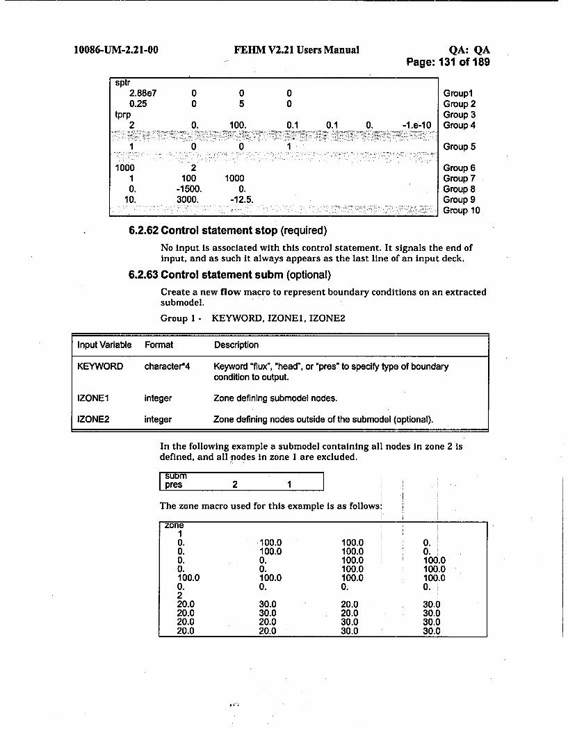
10086-UM-2.21-0O FEHM V2.21 Users Manual QA: QAPage: 131 of 189
Group1Group 2Group 3
-1.e-10 Group 4
Group 5
Group 6Group 7Group 8Group 9Group 10
6.2.62 Control statement stop (required)
No input is associated with this control statement. It signals the end ofinput, and as such it always appears as the last line of an input deck.
6.2.63 Control statement subm (optional)
Create a new flow macro to represent boundary conditions on an extractedsubmodel.
Group 1 - KEYWORD, IZONE1, IZONE2
Input Variable Format Description
KEYWORD character*4 Keyword "flux", "head", or "pres" to specify type of boundary
condition to output.
IZONE1 integer Zone defining submodel nodes.
IZONE2 integer Zone defining nodes outside of the submodel (optional).
In the following example a submodel containing all nodes in zone 2 isdefined, and all nodes in zone 1 are excluded.
SUDmpres 2 1
The zone macro used for this example is as follows;
zone10. 100.0 100.0 0.0. 100.0 100.00. 0. 100.0 100.00. 0. 100.0 100.0100.0 100.0 100.0 100.00. 0. 0. 0.220.0 30.0 20.0 30.020.0 30.0 20.0 30.020.0 20.0 30.0 30.020.0 20.0 30.0 30.0

10086-UM-2.21-OO FEHM V2.21 Users Manual QA: QAPage: 132 of 189
.Uu.u 1UU.U .U 1 UU.U99.0 99.0 99.0 99.0360.0 90.0 90.0 60.060.0 90.0 90.0 60.060.0 60.0 90.0 90.060.0 60.0 90.0 90.01.0 1.0 1.0 1.00.0 0.0 0.0 0.0
The code produces the following "flow" macro output for this example:
flow Boundary Conditions Output: FEHM V2.21 sun 03-07-26 7/29/2003 10:47:50336 336 1 1.43112776 1.0 1.OE+02 # 22.5000 27.5000 100.000337 337 1 1.42620726 1.0 1.OE+02 # 27.5000 27.5000 100.000358 358 1 1.43081773 1.0 1.OE+02 # 22.5000 22.5000 100.000
.359 359 1 1.42601577 1.0 1.OE+02 # 27.5000 22.5000 100.000
6.2.64 Control statement svar (optional)Group I - IVAR
Input Variable Format Description
WAR integer To enable pressure-enthalpy variables in place of pressuretemperature for water/water vapor physics IVAR = 1. Default isdisabled.
6.2.65 Control statement szna or napl (optional)
Group 1 - ICO2D
Group 2 - TREF, PREF
Group 3- DENNAPL, VISCNAPL
Input Variable Format Description
ICO2D integer Determines the type of air module used.ICO2D = 1, 1 degree of freedom solution to the saturated-unsaturated
problem is produced. This formulation is similar to the Richard'sEquation.
ICO2D = 2, 1 degree of freedom solution is obtained assuming onlygas flow with no liquid present.
IC02D = 3, full 2 degree of freedom solution.All other values are Ignored. The default is 3.
TREF real Reference temperature for properties (°C).
PREF real Reference pressure for properties (MPa).
DENNAPL real NAPL density (kg/m 3 ).
VISCNAPL real NAPL viscosity (Pa s).

10086-UM-2.21-00 FEHM V2.21 Users Manual QA: QAPage: 133 of 189
The following is an example of szna. In this example, a full 2-degrees-of-freedom solution is specified with a reference temperature for propertyevaluation of 20 °C and a reference pressure of 0.1 MPa. The NAPL densityis 800 kg/m 3 and the viscosity is 5.e-3 Pa. s.
szna3
20. 0.1800. 5.e-3
6.2.66 Control statement-text (optional)
Group 1- WDD1
Input Variable Format Description
WDD1 character*80 Line of text. A maximum of 80 characters per line are entered. Text isinput until a blank line is inserted to signal the end of the controlstatement. This text is written to the output file (iout).
The following is an example of texttext
This 2-d model of the PACE problem will be used to study thermal effects.user # = -20 to get waste packages
6.2.67 Control statement thic (optional)
Input for variable thickness for two-dimensional problems.
Group 1 - JA, JB, JC, THIC (JA, JB, JC - defined on page 31).
Input Variable Format Description
THIC real Thickness of the model domain in the third dimension(m). Default is 1.
The following is an example of thic. In this example, the thickness for allnodes is set to 10 m, after which the nodes defined by zone 2 are set to 5 m.Thus, the thickness is 10 m everywhere except zone 2, where thickness is5 m.
thic1 0 0 10.
-2 0 0 5.
6.2.68 Control statement time (required)
Time step and time of simulation data.
Group 1 - DAY, TIMS, NSTEP, IPRTOUT, YEAR, MONTH, INITTIME
Group 2 - DITI, DIT2, DIT3, ITC, DIT4 (as needed)

10086-UM-2.21-00 FEHM V2.21 Users Manual QA: QAPage: 134 of 189
DAY should be larger than DAYMIN defined in control statement ctrl. Thecode proceeds to the next control statement when a blank line isencountered for Group 2. Group 2 can be used to generate output at specifictimes (with multiple Group 2s). Contour plot output will be written at eachDITI regardless of the input in control statement cont. The restart file willbe written (or rewritten if one already exists) at each DITI. If DIT4 isomitted (for compatibility with older input files where DIT4 was not input)the maximum time step defined in the control statement ctrl will be used.
Input Variable Format Description
DAY real Initial time step size (days).
TIMS real Final simulation time (days).
NSTEP integer Maximum number of time steps allowed.
IPRTOUT integer Print-out interval for nodal information (pressure, enthalpy etc.), asset up under control statement node. (i.e., number of time steps).
YEAR integer Year that simulation starts.
MONTH integer Month that simulation starts.
INITTIME real Initial time of simulation (days). For compatibility with older versions,if this parameter is absent the initial time of simulation will be 0 if norestart file is used, or the time in the restart file if one is used.
DIT1 real Time (days) fortime step change.
DIT2 real New time step size (days). If DIT2 < 0 then ABS (DIT2) is the newtime step multiplier.
DIT3 real Implicitness factor for new time step.DIT3 < 1.0 backward Euler.DIT3 > 1.0 for second-order Implicit scheme.
ITC integer New print-out interval.
DIT4 real Maximum time step size for next time interval (days).
The following is an example of time. In this example, the initial time stepsize is 30 days, the final simulation time is 3650 days, the number of timesteps allowed is 20, nodal information is printed out for every 5th timestep, the simulation starts in the 10th month of 1989, and the initial timeof simulation is assigned a value of 0. The time step multiplier is changedafter 1 day, and the new time step multiplier is 1.2, backward Euler is usedfrom this time on and the printout interval is every 10th time step. Themaximum time step size for the next interval is omitted so the defaultvalue entered in the ctrl macro will be used.
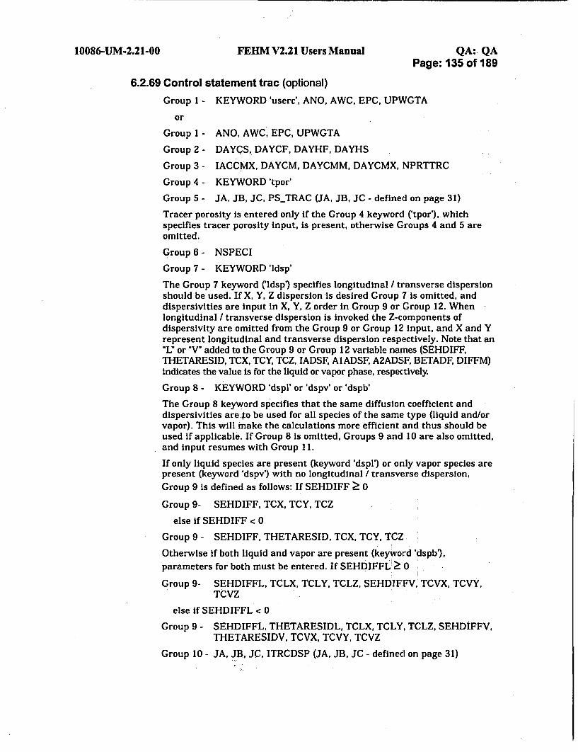
10086-UM-2.21-00 FEHM V2.21 Users Manual QA: QAPage: 135 of 189
6.2.69 Control statement trac (optional)
Group I - KEYWORD 'userc', ANO, AWC, EPC, UPWGTA
or
Group 1 - ANO, AWC, EPC, UPWGTA
Group 2 - DAYCS, DAYCF, DAYHF, DAYHS
Group 3 - IACCMX, DAYCM, DAYCMM, DAYCMX, NPRTTRC
Group 4 - KEYWORD'tpor'
Group 5 - JA, JB, JC, PS_TRAC (JA, JB, JC - defined on page 31)
Tracer porosity is entered only if the Group 4 keyword ('tpor'), whichspecifies tracer porosity Input, is present, otherwise Groups 4 and 5 areomitted.
Group 6 - NSPECI
Group 7 - KEYWORD'ldsp'
The Group 7 keyword ('ldsp') specifies longitudinal / transverse dispersionshould be used. If X, Y, Z dispersion is desired Group '7 is omitted, anddispersivities are input in X, Y, Z order in Group 9 or Group 12. Whenlongitudinal / transverse dispersion is invoked the Z-components ofdispersivity are omitted from the Group 9 or Group 12 input, and X and Yrepresent longitudinal and transverse dispersion respectively. Note that an"L" or W" added to the Group 9 or Group 12 variable names (SEHDIFF,THETARESID, TCX, TCY, TCZ, IADSF, A1ADSF, A2ADSF, BETADF, DIFFM)indicates the value is for the liquid or vapor phase, respectively.
Group 8 - KEYWORD 'dspl' or 'dspv' or 'dspb'
The Group 8 keyword specifies that the same diffusion coefficient anddispersivities are .o be used for all species of the same type (liquid and/orvapor). This will make the calculations more efficient and thus should beused if applicable. If Group 8 is omitted, Groups 9 and 10 are also omitted,and input resumes with Group 11.
If only liquid species are present (keyword 'dspl') or only vapor species arepresent (keyword 'dspv') with no longitudinal / transverse dispersion,Group 9 is defined as follows: If SEHDIFF > 0
Group 9- SEHDIFF, TCX, TCY, TCZ
else if SEHDi FF < 0
Group 9 - SEHDIFF, THETARESID, TCX, TCY, TCZ
Otherwise if both liquid and vapor are present (keyword 'dspb'),parameters for both must be entered. If SEHDIFFL! Ž 0
Group 9- SEHDIFFL, TCLX, TCLY, TCLZ, SEHDIFFV, TCVX, TCVY,TCVZ
else if SEHDIFFL < 0
Group 9 - SEHDIFFL, THETARESIDL, TCLX, TCLY, TCLZ, SEHDIFFV,THETARESIDV, TCVX, TCVY, TCVZ
Group 10 - JA, JB, JC, ITRCDSP (JA, JB, JC - defined on page 31)

10086-UM-2.21-00 FEHM V2.21 Users Manual QA: QAPage: 136 of 189
Group 11 - ICNS
There are two options for group twelve. If the same diffusion coefficient anddispersivities are to be used for all species of the same type (liquid and/ orvapor - keyword 'dspl', 'dspv', or 'dspb') only sorption parameters are input:
Group 12 -IADSF, A1ADSF, A2ADSF, BETADF
or for a Henry's Law Species (both liquid and vapor)
Group 12- IADSFL, AIADSFL, A2ADSFL, BETADFL, IADSFV,AIADSFV, A2ADSFV, BETADFV
In the absence of a Group 8 keyword ("dspl', 'dspv', or 'dspb') the followinginput (for liquid or vapor) which includes the sorption and dispersionparameters is used: If DIFFM >_ 0
Group 12 - IADSF, AIADSF, A2ADSF, BETADF, DIFFM, TCX, TCY, TCZ
else if DIFFM < 0
Group 12 - IADSF, AIADSF, A2ADSF, BETADF, DIFFM, THETARESID,TCX, TCY, TCZ
For a Henry's Law Species (both liquid and vapor) if DIFFML Ž- 0
Group 12 - IADSFL, AIADSFL, A2ADSFI, BETADFL, DIFFML, TCLX,TCLY, TCLZ, IADSFV, AIADSFV, A2ADSFV, BETADFV,DIFFMV, TCVX, TCVY, TCVZ
else if DIFFML < 0
Group 12 - IADSFL, A1ADSFL, A2ADSFL, BETADFL, DIFFML,THETARESIDL, TCLX, TCLY, TCLZ, IADSFV, A1ADSFV,A2ADSFV, BETADFV, DIFFMV, THETARESIDV, TCVX,TCVY, TCVZ
Group 13 - JA, JB, JC, ITRCD (JA, JB, JC - defined on page 31)
Group 14 - HENRY-MODEL, HAWWA(1), HAWWA(2), HAWWA(3),HAWWA(4), HAWWA(5) (only input for a Henry's Law species,otherwise omitted)
Group 15 - JA, JB, JC, ANQO (JA, JB, JC - defined on page 31)
Group 16 - JA, JB, JC, CNSK, T1SK, T2SK (JA, JB, JC - defined onpage 31)
Groups 11, 12, t-3, 14, 15, and 16 are entered as a unit for each solute.However, for a solid species, only groups 11, 15, and 16 are entered (groups12, 13, and 14 are not applicable for a solid species). Groups 12 and 13 areused to define transport models for which sorption and dispersionparameters are identical. For a liquid or vapor species, only one set ofGroup 12 parameters should be entered per region. However, for a Henry'sLaw species, two sets of parameters per region must be entered. For thiscase, the liquid sorption parameters should be entered on the first line andthe vapor sorption parameters on a second line or as a continuation of thefirst line. Group 12 is read in until a blank line is encountered. The modelnumber is incremented by 1 each time a line is read. Group 13 then assignsa transport model number to every node.

10086-UM-2.21-00 FEHM V2.21 Users Manual QA: QAPage: 137 of 189
Injection nodes must be specified in control statement flow.
Input Variable Format Description
KEYWORD
ANO
AWC
EPC
UPWGTA
DAYCS
DAYCF
DAYHF
DAYHS
IACCMX
DAYCM
DAYCMM
DAYCMX
NPRTTRC
KEYWORD
PSTRAC
NSPECI
character*5 Keyword for invoking a solute transport user subroutine. If the wordIuserc' is placed in this position, then the code Invokes a solutetransport user subroutine at each time step. Omit this key word ifthere is no solute user subroutine for the simulation.
real Initial solute concentration, set at all nodes for all species unlessoverwritten by a restart file input or values in group 14 below(moles/kg fluid).
real Implicitness factor for solute solution.AWC > 1.0 gives 2nd order solutionAWC < 1.0 gives 1st order solution
real Equation tolerance for solute solution. When the square root of thesum of the squared residuals is lower than EPC, the solution isassumed to be converged.
real Upstream weighting term for the solute solution.UPWGTA < 0.5 UPWGTA is set to 0.5UPWGTA > 1.0 UPWGTA is set to 1.0
real Time which the solute solution is enabled (days).
real Time which the solute solution is disabled (days).
real Time which the flow solution is disabled (days).
real Time which the flow solution is enabled (days).
Integer Maximum number of iterations allowed in solute solution if timestep multiplier is enabled
real Time step multiplier for solute solution
real Initial time step for solute solution (days)
real Maximum time step for solute solution (days)
integer Print-out interval for solute information. Data for every NPRTTRCsolute time step will be written to the "trc" file. If this parameter isomitted (for compatibility with old input files) the default value is 1.Note that the first and last solute time step within a heat and masstransfer step automatically get printed.
character*4 Keyword 'tpor' specifying optional tracer porosity should be input. If
group 4 is omitted, porosities assigned in macro rock are used.
real Tracer porosity
integer Number of solutes simulated.

10086-UM-2.21-00 FEHM V2.21 Users Manual QA: QAPage: 138 of 189
Input Variable Format Description
KEYWORD character*4 Keyword 'Idsp' specifying longitudinal I transverse dispersion. If x,y, z dispersion is desired group 7 is omitted, and dispersivities areinput in x, y, and then z order (group 9 or group 12). Otherwise, iflongitudinal / transverse dispersion is desired the keyword 'Idsp' isentered and dispersivities are instead input in longitudinal and thentransverse order with values for the third dimension omitted.
KEYWORD character*4 Keyword specifying the same diffusion coefficient anddispersivities are to be used for all species of the same type (liquidand/or vapor).
'dspl' indicates that only liquid species exist.'dspv' indicates that only vapor species exist.'dspb' indicates that both liquid and vapor species exist.
ICNS integer Phase designation for the ith solute-2 - Henry's Law species (input and output concentration values
are gas concentrations).-1 - Vapor species.0 - Solid species1 - Liquid species2 - Henry's Law species (input and output concentration values
are liquid concentrations)
SEHDIFF real Molecular diffusion coefficient (m2/s)If SEHDIFF > 0, the molecular diffusion coefficient Is a constant.If SEHDIFF < 0, this indicates the model of Conca and Wright(1992) for diffusion coefficient as a function of volumetric watercontent is used, and ABS(SEHDIFF) is the diffusion coefficient atsaturation equal to one, and THETARESID is the water content atwhich the diffusion coefficient reaches a low value.
THETARESID real Residual water content for Conca and Wright function.
TCX real Dispersivity in x-direction (m)
TCY real Dispersivity in y-direction (m)
TCZ real Dispersivity in z-direction (m)
ITRCDSP integer Region number for dispersion parameters given in group 9(keyword). Default is 1.
IADSF integer Adsorption model type for the ith species, Ith region0 - conservative solute1 - linear sorption isotherm2 - Freundlich sorption isotherm3 - Modified Freundlich sorption isotherm4 - Langmuir sorption isotherm
A1ADSF real a, parameter in adsorption model
A2ADSF real a2 parameter in adsorption model
BETADF real 0 parameter in adsorption modelBETADF real f3 parameter in adsorption model

10086-UM-2.21-00 FEIM V2.21 Users Manual QA: QAPage: 139 of 189
Input Variable Format Description
DIFFM real Molecular diffusion coefficient (m2/s) See discussion for SEHDIFF.
ITRCD integer Region number for group 12 sorption parameters or for sorptionand dispersion parameters (no keyword). Default is 1.
HENRY-MODEL integer Flag denoting which model is to be used for defining thetemperature dependence of the Henry's law constant
1 - van't Hoff model2 - Multi-parameter fit to experimental data (used for carbonate
system).
HAWWA(1) real Term in Henry's Law temperature dependence model:For model 1 - parameter value is AHFor model 2 - parameter value is AH,1
HAWWA(2) real Term in Henry's Law temperature dependence model:For model 1 - parameter value is AHH
For model 2 - parameter value is AH,2
HAWWA(3) real Term in Henry's Law temperature dependence model:For model 1 - not usedFor model 2 - parameter value Is AH,3
HAWWA(4) real Term in Henry's Law temperature dependence model:For model I - not usedFor model 2 - parameter value is AH,4
HAWWA(5) real Term in Henry's Law temperature dependence model:For model 1 - not usedFor model 2 - parameter value is AH,5
ANQO real Initial concentration of tracer, which will supersede the value givenin group 1. Note that if initial values are read from a restart file,these values will be overwritten. Units are moles per kg vapor orliquid for a liquid, vapor, or Henry's law species, and moles per kgof solid for a solid species. Default is 0.
CNSK real Injection concentration at inlet node (moles per kg liquid or vapor).If fluid is exiting at a node, then the in-place concentration is used.If CNSK < 0, then the concentration at that particular node will beheld at a concentration of abs(cnsk) (default is 0 for all unassignednodes).
T1SK real Time (days) when tracer injection begins. Default is 0.TISK real Time (days) when tracer injection begins. Default is 0.
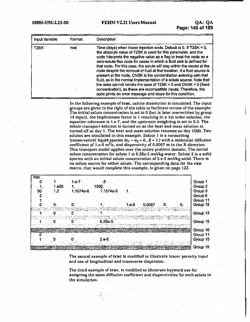
------ mm
10086-UM-2.21-00 FEHM V2.21 Users Manual QA: QAPage: 140 of 189
Input Variable Format Description
T2SK real Time (days) when tracer injection ends. Default is 0. If T2SK < 0,the absolute value of T2SK is used for this parameter, and thecode interprets the negative value as a flag to treat the node as azero-solute-flux node for cases in which a fluid sink is defined forthat node. For this case, the solute will stay within the model at thenode despite the removal of fluid at that location. If a fluid source ispresent at the node, CNSK is the concentration entering with thatfluid, as in the normal implementation of a solute source. Note thatthe code cannot handle the case of T2SK < 0 and CNSK < 0 (fixedconcentration), as these are incompatible inputs. Therefore, thecode prints an error message and stops for this condition.
In the following example of trac, calcite dissolution is simulated. The inputgroups are given to the right of the table to facilitate review of the example.The initial solute concentration is set to 0 (but is later overwritten by group14 input), the implicitness factor is I resulting in a 1st order solution, theequation tolerance is 1.e-7, and the upstream weighting is set to 0.5. Thesolute transport solution is turned on as the heat and mass solution isturned off at day 1. The heat and mass solution resumes on day 1000. Twosolutes are simulated in this example. Solute I is a nonsorbing(conservative) liquid species (a, = a2 = 0., J3 = 1.) with a molecular diffusioncoefficient of 1.e-9 m2/s, and dispersivity of 0.0067 m in the X-direction.This transport model applies over the entire problem domain. The initialsolute concentration for solute 1 is 6.26e-5 mol/kg-water. Solute 2 is a solidspecies with an initial solute concentration of 2.e-5 mol/kg-solid. There isno solute source for either solute. The corresponding data for the rxnmacro, that would complete this example, is given on page 122.
trac0 1 1.e-7 .5 Group I1. 1.e20 1. 100.. Group 2
50 1.2 1.1574e-6 1.1 574e-3 1 Group 32 Group 61 Group 110 0. 0. 1. 1.e-9 0.0067 0. 0. Group 12
1 0 0 1 Group 13
1 0 0 6.26e-5 Group 15
Group 11
1 0 0 2.e-5 Group 15
Group 16
The second example of trac is modified to illustrate tracer porosity inputand use of longitudinal and transverse dispersion.
The third example of trac, is modified to illustrate keyword use forassigning the same diffusion coefficient and dispersivities for each solute inthe simulation.

10086-UM-2.21-00 FEIIM V2.21 Users Manual QA: QAPage: 141 of 189
Group 1Group 2Group 3Group 4Group 5
Group 6Group 7Group 11
0.0067 Group 12
Group 13
Group 15
Group 11Group 15
G Group 1
Group 2Group 3Group 6Group 8Group 9Group 1Group 19
Group 12Group 13
Group 15Group 16
Group 15
Group 15Group 16
Group 16
trac;trac0 1 1.e-7 .5
1. 1.e20 1. 1000.50 1.2 1.1574e-6 1.1574e-3 12
dspl1 .e-9 0.0067 0.0067 0.00671 0 0 1
10 0. 0. 1.
1 0 0 1
0 0 6.26e-5
01 0 0 2.e-5
The final example of trac illustrates use of the "userc" subroutine andapplies only to the version of this subroutine that is included/compiled withthe current version of FEHM. The user subroutine is invoked from the tracmacro using the keyword *userc" in Group 1. When invoked, the code looksfor an additional data file "userc_data.dat" in the current workingdirectory, in which the following input is required:
Group 1 - USROPTION (integer)The only option currently supported is option 2: Time-varyingsolute mass flux input at prescribed nodes.
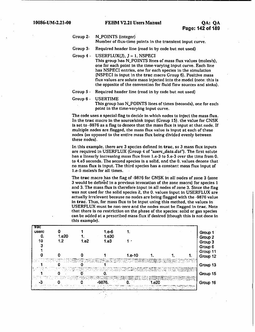
10086-UM-2.21-00 FEHM V2.21 Users Manual QA: QAPage: 142 of 189
Group 2- N_POINTS (integer)
Number of flux-time points in the transient input curve.
Group 3- Required header line (read in by code but not used)
Group 4 - USERFLUX(J), J = 1, NSPECIThis group has N_POINTS lines of mass flux values (moles/s),one for each point in the time-varying input curve. Each linehas NSPECI entries, one for each species in the simulation(NSPECI is input in the trac macro Group 6). Positive massflux values are solute mass injected into the model (note: this isthe opposite of the convention for fluid flow sources and sinks).
Group 5 - Required header line (read in by code but not used)
Group 6- USERTIMEThis group has NPOINTS lines of times (seconds), one for eachpoint in the time-varying input curve.
The code uses a special flag to decide in which nodes to inject the mass flux.In the trac macro in the source/sink input (Group 15), the value for CNSKis set to -9876 as a flag to denote that the mass flux is Input at that node. Ifmultiple nodes are flagged, the mass flux value is input at each of thesenodes (as opposed to the entire mass flux being divided evenly betweenthese nodes).
In this example, there are 3 species defined in trac, so 3 mass flux inputsare required in USERFLUX (Group 4 of "userc..data.dat"). The first solutehas a linearly increasing mass flux from 1.e-3 to 5.e-3 over the time from 0.to 4.e5 seconds. The second species is a solid, and the 0. values denote thatno mass flux is input. The third species has a constant mass flux input of1.e-5 moles/s for all times.
The trac macro has the flag of -9876 for CNSK in all nodes of zone 3 (zone3 would be defined in a previous invocation of the zone macro) for species 1and 3. The mass flux is therefore input in all nodes of zone 3. Since the flagwas not used for the solid species 2, the 0. values input in USERFLUX areactually irrelevant because no nodes are being flagged with the -9876 valuein trac. Thus, for mass flux to be input using this method, the values inUSERFLUX must be non-zero and the nodes must be flagged in trac. Notethat there is no restriction on the phase of the species: solid or gas speciescan be added at a prescribed mass flux if desired (though this is not done inthis example).
tracuserc 0 1 1.e-6 1. Group 1
0. 1.e20 1. 1.e30 Group 210 1.2 1.e2 1.e3 1 Group 3
3 Group 61 Group 110 0 0 1 1.e-10 1. 1. 1. Group 12
1 0 0 1 Group 13
1 0 0 0. Group 15
Group 16

10086-UM-2.21-0O FEHM V2.21 Users ManualPage: 1
01 0 0 0.
0 0 0 1 I.e-10 1
1 0 0 1
1 0 0 0.
-3 0 0 -9876. 0. 1 .e20
File "userc_data.dat":
QA: QA43 of 189
Group 11Group 15
Group 16Group 11Group 12
Group 13
Group 15
Group 6
25
Mass flux (moles/s)1.e-3 0. 1.e-52.e-3 0. I.e-53.e-3 0. 1.e-54.e-3 0. 1.e-55.e-3 0. 1.e-5
Time (seconds)0.1 .e52.e53.e54.e5
Group 1Group 2Group3Group 4
Group 5Group 6
A final point needing explanation is the use of times T1SK and T2SK inGroup 15 of trac. These values are times (in days, as opposed to theseconds used for USERTIME in Group 6 of usercdata.dat) defining theinterval over which source/sink values are used. The normal logic of thecode is still used to decide whether a source or sink is employed, namelythat the source/sink term is only present between T1SK and T2SK.Therefore, the time-varying input must fall between T1SK and T2SK: anyportion of the simulation outside of this range will have no source/sinkregardless of the input in "userc_data.dat". Practically speaking, settingthe values of T1SK and T2SK to 0. and L.e20 days (very large),respectively, will ensure that the entire span of times in userc-data.dat isused for the mass flux input, and the source is not shut off during thesimulation.

10086-UM-2.21-00 FEHM V2.21 Users Manual QA: QAPage: 144 of 189
6.2.70 Control statement user (optional)
Group 1 - KK
Input Variable Format Description
KK integer Integer number passed to subroutine user for user defined Inputparameters. This user subroutine call differs from the one invoked inthe control file In that whereas that subroutine is called at every timestep, this one is called only at the beginning of the simulation to setparameters that do not change later in the simulation.
The following is an example of user. In this example, the number 5 ispassed to the user subroutine.luser
6.2.71 Control statement vapl (optional)
Enable vapor pressure lowering. For more information see the "Models andMethods Summary" of the FEHM Application [Zyvoloski et al. 1999,Equation (127), page 62]. No input is associated with this macro.
6.2.72 Control statement vcon (optional)
Variable thermal conductivity information.
Group 1 - IVCON(i), VC1F(i), VC2F(i), VC3F(i)
Group 2 - JA, JB, JC, IVCND (JA, JB, JC - defined on page 31)
The parameter (i) is incremented each time Group 1 is read. Group 2 lineswill refer to this parameter. Group 1 is ended with a blank line.
Input Variable Format Description
IVCON(i) integer Model type for ith conductivity model.IVCON(i) = 1, linear variation of thermal conductivity with
temperature.IVCON(i) = 2, square root variation of thermal conductivity with
liquid saturation.
VCIF(i) real Reference temperature (°C) for IVCON(i) = 1. Conductivity ( -Wat liquid saturation = 1 for IVCON(i) = 2.
VC2F(i) real Reference conductivity ( 2L ) for IVCON(i):: 1. Conductivity
( at liquid saturation = 0 for IVCONi) %:2.VC3F(i) real Change in conductivity with respect to temperature for IVCON(i) = e.
Not used for IVCON(i) = 2.
IVCND integer Number referring to the sequence of models read in Group Il. Thedefault is 1.
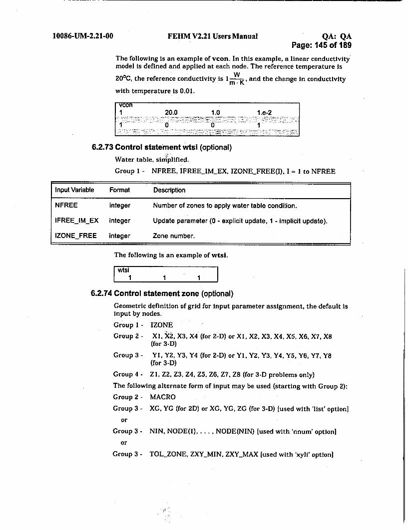
10086-UM-2.21-00 FEHM V2.21 Users Manual QA: QAPage: 145 of 189
The following is an example of vcon. In this example, a linear conductivitymodel is defined and applied at each node. The reference temperature isW20 0 C, the reference conductivity is 1 W , and the change in conductivity
with temperature is 0.01.
6.2.73 Control statement wtsi (optional)
Water table, simplified.
Group 1 - NFREE, IFREEIMEX, IZONEFREE(I), I = 1 to NFREE
Input Variable Format Description
NFREE integer Number of zones to apply water table condition.
IFREEIMEX integer Update parameter (0 - explicit update, 1 - implicit update).
IZONEFREE integer Zone number.
The following is an example of wtsi.
wtsi1I
6.2.74 Control statement zone (optional)
Geometric definition of grid for input parameter assignment, the default isinput by nodes.
Group 1 - IZONE
Group 2 - Xl, k2, X3, X4 (for 2-D) or X1, X2, X3, X4, X5, X6, X7, X8(for 3-D)
Group 3 - Yl, Y2, Y3, Y4 (for 2-D) or Yl, Y2, Y3, Y4, Y5, Y6, Y7, Y8(for 3-D)
Group 4 - ZI, Z2, Z3, Z4, Z5, Z6, Z7, Z8 (for 3-D problems only)
The following alternate form of Input may be used (starting with Group 2):
Group 2 - MACRO
Group 3 - XG, YG (for 2D) or XG, YG, ZG (for 3-D) [used with 'list' option]
or
Group 3 - NIN, NODE(l), ... NODE(NIN) [used with 'nnum' option]
or
Group 3 - TOLZONE, ZXYMIN, ZXYMAX [used with 'xyli' optioni

10086-UM-2.21-00 FEHM V2.21 Users Manual QA: QAPage: 146 of 189
Group 4 - XG,:YG [used with 'xyli' option]
Input Variable Format Description
IZONE integer Zone identification number for geometric input.
XI-X8 real X coordinates defining zone IZONE (m).
Y1-Y8 real Y coordinates defining zone IZONE (m).
ZI-Z8 real Z coordinates defining zone IZONE (m).
MACRO character*4 String denoting alternate input formatMACRO = "list", read a list of X, Y, Z - coordinates, one set per line
until a blank line is encountered. The nodes corresponding tothese coordinates make up the zone.
MACRO = "nnum", read the number of specified nodes, followed bythe node numbers. These comprise the zone.
MACRO = *xyli", read a column radius, followed by a list of X, Y -coordinates, one set per line until a blank line is encountered.The nodes contained in columns centered on each x, y pair andextending to the defined boundaries in the Z direction make upthe zone. The column radius is necessary because there are(usually) slight variations in the Z direction of nodes above andbelow the prescribed X, Y coordinates.
XG real X coordinate of node to be included in IZONE (m).
YG real Y coordinate of node to be included in IZONE (m).
ZG real Z coordinate of node to be included in IZONE (m).
NIN integer Number of nodes in IZONE.
NODE(i) integer NIN node numbers of the nodes to be included in IZONE.
TOLZONE real Column radius (m).
ZXYMIN real Minimum Z coordinate for XY list (m).
ZXYMAX real Maximum Z coordinate for XY list (m).
The geometric zone description Is implemented by defining geometricregions. The coordinates given in Group 2, 3, and 4 refer to node positionsshown in Fig. 2. All properties defined by node (JA, JB, JC) in any controlstatements may be defined by zone. In the previous macro descriptions IfJA < 0, then the zone IZONE = ABS (JA) is referenced.
It is a good policy to refer to the input check file to insure that nodeassignments haye been made as expected. When X, Y, Z coordinates areused to define zones, boundaries of those zones may be slightly differentthan specified. This is due to the Inclusion of volume from elementsadjoining included nodes.
When macro statements dpdp and dual are used, additional zonedefinitions are automatically generated. These are identified by zones 101-200 for the first set of matrix nodes and 201-300 for the second set of

10086-UM-2.21-00 FEHM V2.21 Users Manual QA: QAPage: 147 of 189
matrix nodes. For example, Zone 101 corresponds to the matrix materialoccupying the same space occupied by the fracture identified by Zone 1.Furthermore, Zone 201 refers to the second matrix layer in the dualcontrol statement. Zones for the dpdp and dual matrix nodes may beexplicitly defined and will not be superseded by automatically generatedzones.
The macro zone must precede the usage of a ZONE reference. zone isended with a blank line. zone can be called more than once and regionsredefined. When this is done, all previous zone definitions are eliminated.A node may be included in only a single zone at a time.
The following are examples of zone. In the first example, 8 zones (for a 2-Dproblem) are defined, zone 1 is all the nodes that lie within the areabounded by the f6ur points with X, Y coordinates given by (0.,1075.),(1000., 1074.), (1000.,1079.) and (0., 1080.) and similarly for zones 2 - 6.Zone 7 is defined using the "nnum" keyword and consists of a single node,100. Zone 8 is defined using the "list" keyword and consists of the singlenode closest to coordinates (0., 0.).
zone1 . I0.00 1000.00 1000.00 0.00
1075.00 1074.00 1079.00 1080.0020.000 1000.00 1000.00 0.00
870.000 869.000 1074.00 1075.0030.000 1000.00 1000.00 0.000
860.000 859.000 869.000 870.00040.000 1000.00 1000.00 0.000
780.000 779.000 859.000 860.00050.000 1000.00 1000.00 0.000
730.000 730.000 780.00060.000 1000.00 1000.00 0.000
700.000 700.000 730.000 730.0007
nnum1 1008
list0. 0.

10086-UM-2.21-00 FEHM V2.21 Users Manual QA: QAPage: 148 of 189
In the second example 2 zones of a 3D problem are defined using "xyli". Thecolumns have a radius of 0.5 m extending from 0 - 1000 m in Z, and arecentered around the nodes closest to the given coordinates.
zone1
xylist0.5 0. 1000.0. 0.0. 1.00. 1.50. 2.00. 3.0
2xylist
0.5 0.1.0 0. 1000.1.0 1.01.0 1.51.0 •2.01.0 3.0
6.2.75 Control statement zonn (optional)
The input for this macro is identical to macro zone, except that previouszone definitions are retained between calls unless specifically overwritten.

10086-UM-2.21-00 FEHM V2.21 Users Manual QA: QAPage: 149 of 189
7.0 OUTPUTOutput is found in the code generated files (output file, write file, history plot file, soluteplot file, contour plot file, contour plot file for dual or dpdp, stiffness matrix data file,input check file, submodel output file, PEST output files, streamline particle trackingoutput files, and AVS output files) described in Section 5.0.Macro commands (input options) dealing with output control are cont (page 45), ctrl(page 48), nod2 (page 85), node (page 85), mptr (page 75), pest (page 88), ptrk (page 91),sptr (page 124), and time (page 133): cont is used to specify output format and timeintervals for contour data output (fehmn.con, fehmn.dp); ctrl is used to specify ifelement coefficients calculated in the code should be saved (fehmn.stor); node and nod2are used to provide nodal or coordinate positions for which general information andhistory data will be output (fehmn.out, fehmn.his, fehmn.trc, and terminal output);mptr has an option to specify whether or not particle tracking information is written tothe restart file (fehmn.fin); pest is used to specify PEST parameter estimation routineoutput format (fehmn.pest, fehmn.pestl); ptrk has an option to specify whether or notparticle tracking information is written to the restart file (fehmn.fin) and whatinformation to output; sptr has options to specify what streamline particle trackinginformation will be output (fehmn.sptrl, fehmn.sptr2, fehmn.sptr3); subm is used tospecify nodes and boundary conditions should be output for an extracted submodelregion; and time provides input on the time printout interval for nodal information(fehmn.out and terminal output).The code itself provides no graphical capabilities. History plots of the energy source,source strength, temperature, pressure, capillary pressure, and saturation are madefrom the filen.his FEHM output files. Data from the filen.trc files is used to makehistory tracer plots of the 10 species concentrations. Contour plots can be made from thefilen.con, fllen.dp, and AVS FEHM output files.AVS provides tools for visualization and analysis of volumetric scalar and vector dataContour plots using 2-d quad. grids and 3-d hex grids for material properties,temperature, saturation, pressure, velocities, and solute concentrations can be made.The plots can be rotated, zoomed, scaled, translated, and printed. Axis values and thecolor bar can be customized. AVS FEHM output files are available for the following nodedata: material properties, liquid and vapor phase values, velocity and pressure values,temperature, saturation, concentrationand, and for the dua and dpdp models. The AVSoutput files from FEHM are written in an ASCII format that can be imported into AVSUCD graphics routines for viewing.Additional information on the data found in the output files is given below.
7.1 Output file (filen.out)Information contained in the general output file is mostly self explanatory. Thefile starts with the code version, date, and time followed by the user input problemtitle. A summary of the I/O files used, macro control statements read, and arraystorage follow. Variable information for user specified nodes at user selected timeintervals is written. The file ends with a summary of simulation time, number oftime steps in the problem, the number of iterations taken, and total cpu time.
7.2 Write file (filen.fin)The write file contains the final values of pressure, temperature, saturation, andsimulation time for the run. The final version of the file is generally written at theend of the simulation. This information is also written if the minimum usersupplied time step has been realized and execution is terminated. If the write file

10086-UM-2.21-OO FEHM V2.21 Users Manual QA: QAPage: 150 of 189
has not been specified at startup the code will use fehmn.fin. The primary use ofthe write file is as a restart file. The write file contains the following:
Code version number, date, time
Problem title
Simulation time (days)
Gas flag [h20 (default), ngas, air]
Tracer flag [trac, ptrk, ntra (default - no output)]
Stress flag [strs, nstr (default - no output)]
Dpdp flag [dpdp, ndpd (default - no output)]
Dual flag [dual, ndua (default - no output)]
If the gas flag is 'h20' (neither air or ngas are set), followed by
Final temperature (*C) at each node
Final saturation (dimensionless) at each node
Final pressure (MPa) at each node
Or if 'ngas' flag is set, followed by
Final temperature (°C) at each node
Final saturation (dimensionless) at each node
Final pressure (MPa) at each node
Final capillary pressure (MPa) at each node
Or if 'air' flag is set, followed by
Final saturation (dimensionless) at each node
Final pressure (MPa) at each node
If 'trac' flag is set followed by
Number of species
Species concentration (vapor or liquid, dimensionless) for each node foreach species
Or if 'ptrk' flag is set followed by
If (ABS (PRNT RST) = 2) (see PRNTRST description in the PTRK macro)
Label: mass flux Values -
Number of mass flux values
Mass flux value (kg/s) for each connection of each node, starting with node1. Note: mass flux values for the fracture domain are listed first followed bythe mass flux values in the matrix domain. The mass flux between fractureand matrix elements are listed last.
Number of particles, final random number seed
Final node position for each particle. If the value is negative, the particleleft the model domain at a fluid sink at that node.
Fractional time remaining at current node for each particle.

10086-UM-2.21-00 FEHM V2.21 Users Manual QA: QAPage: 151 of 189
Multiplier to the plug flow residence time for each particle at the currentnode position, accounting for dispersion, sorption, and matrix diffusioneffects.
Age for each particle, i.e. the time since the particle entered the system.However, if the particle has left the system, this value is the time that theparticle left the system.
If the random number seed in the file is negative, the arrays for thefractional time remaining and the multiplier to the plug flow time havebeen omitted using the PRNTRST = -1 or PRNT_RST = -2 option (seePRNT_RST description in the PTRK macro). A restart simulation usingthis input file will only approximate the behavior of particles since eachparticle will be assumed to have just entered the node. It is preferable torestart a particle tracking simulation using a file that contains the fullrestart information.
If strs (not Implemented In this version)
If 'dpdp' or 'dual' flag Is set
The above information includes dual porosity/dual permeability nodes.
7.3 History plot file (filen.his)The history plot file contains the following:
Code version number, date, time
Problem title
Gas flag ('ngas', 'airw', or blank)
Tracer flag (trae' or blank)
Stress flag ('strs' or blank)
Number of nodes for which data are output
Node number and X, Y, and Z coordinate (m) of each node for which dataare output
'headings'
Depending on problem flags, 2 lines with field descriptors, Case I (default):
"node flow enthalpy(Mj/kg) flow(kg/s) temperature (deg C) total pressure(Mpa)""capillary pressure (Mpa) saturation (kg/kg)"
or Case 2 (hydraulic head):
"node flow enthalpy(Mj/kg) flow(kg/s) temperature (deg C) hydraulic head(m)"
"total pressure (Mpa) saturation (kg/kg)"
or Case 3 (ngas):"node flow enthalpy(Mj/kg) flow(kg/s) temperature (deg C) total pressure(Mpa)"
"air pressure (Mfpa) capillary pressure (Mpa) saturation (kg/kg) relativehumidity"

10086-UM-2.21-00 FEHM V2.21 Users Manual QA: QAPage: 152 of 189
And for each time step
Time (days) followed by
For Case 1:
Node number, Energy source (MJ/s), Source strength (kg/s), Temperature(°C), Total pressure (MPa), Capillary pressure (MPa), and Saturation(dimensionless) for each specified output node.
For Case 2 (hydraulic head):
Node number, Energy source (MJ/s), Source strength (kg/s), Temperature(0C), Hydraulic head (m), Total pressure (MPa), and Saturation
(dimensionless) for each specified output node.
For Case 3 (ngas):
Node number, Energy source (MJ/s), Source strength (kgls), Temperature(0C), Total pressure (MPa), Air pressure (MPa), Capillary pressure (MPa),
Saturation (dimensionless), and Relative humidity for each specifiedoutput node
7.4 Solute plot file (filen.trc)Solute data is output for the same nodes used for the history plot file. The soluteplot file contains:
Code version number, date, time
Problem title
Number of nodes for which data are output
Node number and X, Y, and Z coordinate (m) of each node for which dataare output
Number of different species/components for tracer solution, Number ofliquid components, Number of immobile components, Number of vaporcomponents, and Number of aqueous complexes
and for each time step and each species
Time (days), species number followed by
Species concentration (dimensionless) for each specified output node.
When particle tracking is used, the concentration can be output In severaldifferent forms (number of particles, number per fluid mass, or number per totalvolume). The choice of which form to use is input in the ptrk macro.
7.5 Contour plot file (filen.con)The contour plot file contains:
Code version number, date, time
Problem title
Tracer ('trac') solution or blank
Stress ('strs') solution or blank
Number of nodes for which data are output
X, Y, and Z coordinate (m) of each node for which data are output

10086-UM-2.21-00 FEHM V2.21 Users Manual -QA: QAPage: 153 of 189
Number of nodes per element, total number of elements
Nodal connectivity information for each node of each element
X, Y, Z permeability (m2) for each node
X, Y, Z thermal conductivity ( ) for each node
Porosity, Rock specific heat (i ), Capillary pressure (MPa) for each
node
Number of degrees 'of freedom per node for the current problem, Directionof gravity in problem, Value of gravity
If tracer solution is present
Number of species
and for each specified time
Time (days), injection phase ( 0 liquid, < 0 vapor) followed by
If injection phase is liquid
Liquid transmissibility / density, Liquid density (kg/m 3), Pressure -Capillary Pressure (MPa), Temperature (°C)
and if tracer solution is present
Species concentration of liquid phase
Or if injection phase is vapor
Vapor transmissibility / density, Vapor density (kg/mr3), Pressure (MPa),Temperature (*C)
and if tracer solution is present
Species concentration of vapor phase.
7.6 Contour plot file for dual or dpdp (filen.dp)The contour plot file for dual or dpdp contains the same information as the regularcontour plot file only the parameter values are for the dual porosity / dualpermeability nodes.
7.7 Stiffness matrix data (filen.stor)The stiffness matrix data file is used to store the finite element coefficients foreach node. It eliminates the need for the code to recompute the coefficients forsubsequent runs. It contains the following:
Code version number, date, time
Problem title
Number of storage locations needed to store geometric input types, Numberof nodes, Size oficonnectivity array
Volume associated with each node
Nodal connectivity information for each connection
Position of geometric coefficient for each connection
10086-UM-2.21-00 FEHM V2.21 Users Manual QA: QAPage: 154 of 189
Diagonal position In connectivity array for each node
Finite element geometric coefficient for each storage location
If stress solution is enabled
Finite element geometric coefficient for each storage location for the stressmodule.
7.8 Input check file (filen.chk)This file contains a summary of input information that may be of use in debuggingor memory management of the code. The positions of maximum and minimumvalues of input parameters and derived quantities are given. Also provided is ananalysis of array storage requirements.
7.9 Submodel output file (filen.subbc)The submodel output file contains "flow" macro data that represents boundaryconditions for an extracted submodel (i.e., the output will use the format of the"flow" input macro). The file contains:
Heading: "flow Boundary Conditions Output:", code version number, date,time
for each submodel node, if boundary type is head or pressure,
Node number, Node number, 1, Head (m) or Pressure (MPa), Impedanceparameter, #, X coordinate, Y coordinate, Z cooordinate
or If boundary type Is flux
Node number, Node number, 1, Flux (kg/s), 0.0d00, #, X coordinate, Ycoordinate, Z cooordinate
A blank line to signal end of flow macro input followed by the file terminationmacro
stop
An example is provided with subm input on page 131.
7.10 Error output file (fehmn.err)This file contains the code version number, date, and time followed by any error orwarning messages Issued by the code during a run.
7.11 Multiple simulations script files (fehmn.pre, fehmn.post)The multiple simulations script file fehmn.pre contains UNIX shell script styleinstructions for pre-processing input data, while the script file fehmn.post containsUNIX shell script style instructions for post-processing data.
7.12 PEST output files (filen.pest, filen.pestl)The PEST output file Is used to output data In a format suitable for use by theParameter Estimation Program (PEST) (Watermark Computing, 1994). The firstfile (filen.pest) contains:
Heading: "PEST Output:", code version number, date, time
First parameter label: "pressures" or "heads"
node number and pressure (MPa) or head (ft) for each specified output node

10086-UM-2.21-00 FEHM V2.21 Users Manual QA: QAPage: 155 of 189
Second parameter label: "saturations"
node number and saturation for each specified output node
Third parameter label: *temperatures"
node number and temperature (°C) for each specified output node
Fourth parameter label: "permeabilities"
node number and x, y, and z permeability (M2) for each specified outputnode
Heading: "Total Flux (kg/s) Leaving Zone (flxz macro option)""Zone Number Source Sink Net Boundary"
zone number, source flux, sink flux, net flux, boundary flux
The second file (filen.pestl) contains:
Heading: "PEST Output:", code version number, date, time
Parameter label: "pressures" or "heads"
node number, relative permeability model used, pressure (MPa) or head (ft),saturation, and temperature (°C) for each specified output node
7.13 Streamline particle tracking output files (filen.sptrl, filen.sptr2,fMlen. sptr3)The streamline particle tracking output files contain information generated duringa streamline particle tracking simulation. Depending on output options selected(macro sptr) zero, one, two or three output files are generated.
When option IPRT > 1, the first file (filen.sptrl) contains:
Code version number, date, time
Problem title
"days=%, Current time of streamline particle tracking iteration (days),streamline particle tracking timestep number for current iteration, and
For each particle:
Particle number, X coordinate of particle, Y coordinate of particle,Z coordinate of particle, Element or node number where the particle islocated
When option IPRTO - 1. the second file (filen.sptr2) contains:
Code version number, date, time
Problem title
Heading: *partiqle.number x y z time porosity saturation permeabilityrock-density pressure temperature zone oldnode new-'node" (Note thatthe heading only includes property titles for the default properties or thoseproperties specified by keyword.)
For each particle:
Particle number, X coordinate of particle, Y coordinate of particle,Z coordinate of particle, Current time that the particle has reached(days), Property value of the unit the particle is residing in for eachspecified keyword [in the following order, if specified: porosity,

10086-UM-2.21-00 FEHM V2.21 Users Manual QA: QAPage: 156 of 189
saturation, permeability (mi2), density (kg/m 3), pressure (MPa),temperature (0C), zone number], Element or node number where theparticle is located, Previous node number
If option "zbtc" is invoked, the third file (filen.sptr3) contains:
Code version number, date, time
Problem title
Heading:" Time,(days) Zonel Particles..."
Time (days), Cumulative number of particles that have arrived at eachspecified zone for breakthrough curve output
7.14 SURFER and TECPLOT output files (surzonenumber.txt,veczonenumber.txt, trczonenumber.txt or teczonenumber.plt,veczonenumber.plt, trczonenumber.plt)The SURFER and TECPLOT output files contain output data (pressure or head,saturations, temperatures, fluxes, permeabilities, saturations, porosities,velocities, and concentrations) for selected locations or nodes in a format suitablefor use by the SURFER (Countouring and 3D Mapping) or TECPLOT plottingprograms. The file data content is the same for either plot program with theexception that the inital heading line is omitted from the SURFER files andheading formats are slightly different. The file names are generated using theoutput zone number (+ 1000) and contour plot number (+ 10000), i.e.surlO01_10001.txt or teclOO_10001.plt. The first file (sur*.txt, or tec*.plt)contains:
Heading (tecplot files only): "TITLE =", Code version number, date, time
For pressure output
Heading: VARIABLES = WX "Y" "Z" "pres" "temp" "px" "py" pz" "sat""node"
ZONE T =", zone number, "Simulation time", simulation time (days)
and for each node
X coordinate (m), Y coordinate(m), Z coordinate(m), Pressure (MPa),Temperature (°C), X permeability (m 2 ), Y permeability (m2), Z permeability(m 2 ), Saturation, Node number
or for head output
Heading: VARIABLES = "X" "Y" "Z" "head" "sat" "source" "px" "py" "pz""por" "node"
ZONE T =", zone number, "Simulation time", simulation time (days)
and for each node
X coordinate (m), Y coordinate(m), Z coordinate(m), Head (m), Saturation,Source flux (kg/s), X permeability (m2), Y permeability (m2), Zpermeability (m2), Porosity, Node number
The second file (vec*.txt, or vec*.plt) contains:
Heading (tecplot files only): "TITLE =", Code version number, date, time
Heading: VARIABLES = "X" "Y" "Z" "Vx" "Vy" "Vz" "node"

10086-UM-2.21-00 FERM V2.21 Users Manual QA: QAPage: 157 of 189
ZONE T =", zone number, "Simulation time", simulation time (days)
and for each node
X coordinate (m), Y coordinate(m), Z coordinate(m), X velocity (m2/s), Yvelocity (m2/s), Z velocity (m2/s), Node number
The third file (trc*.txt, or trc*.plt) contains:
Heading (tecplot files only): "TITLE =", Code version number, date, time
Heading: VARIABLES = ,X" "Y" "Z" "anil" "any" "node'
ZONE T =", zone number, "Simulation time", simulation time (days)
and for each node
X coordinate (m), Y coordinate(m), Z coordinate(m), Liquid concentration,Vapor concentration, Node number
7.15 AVS log output file (filen. 10001_a vs log)The AVS log output file is identical for AVS and AVS Express output. It contains:
Code version number, date
AVS log identifier
Problem title
and for each specified time
AVS output file prefix, Call number, and Time (days)
7.16 AVS header output files (filen.numbertypehead)The AVS ASCII (formatted) header files are identical for AVS and AVS Express output.The data types, "mat", "sca", "vec" or "con", are described in Section 7.18. Theheader files contain:
20 lines of text with information about the FEHM AVS output files. Thetext is followed by a one line AVS UCD file header containing:
number of nodes
number of cells
number of data components for the nodes
number of data components for the cells (currently 0)
number of data components for the model (currently 0)
7.17 AVS geometry output file (fMlen. 1000 l_geo)The ASCII (formatted) geometry file for AVS contains the following:
Node id and X, Y, Z coordinates for each node
Cell Id, Material id, Cell type, and the list of Cell vertices
The ASCII (formatted) geometry file for AVS Express contains one additional lineof data at the beginning of the file, followed by the data specified above:
Number of nodes, Number of elements, 0, 0, 0

10086-UM-2.21-00 FEHM V2.21 Users Manual QA: QAPage: 158 of 189
7.18 AVS data output files (filen.number typenode)All the ASCII (formatted) node data files for AVS contain the following headers:
Number of data components and size of each component
A label/unit string for each data component
followed by for each node
the associated node data (described by data type below).
All the ASCII (formatted) node data files for AVS Express contain the followingheaders, on a single line delimited by * : " :
Current simulation time (with format "nodes at time days")
A label/unit string for each data component
followed by for each node
the associated node data (described by data type below), delimited by" :
7.18.1 Material properties (mat andmatdual)
These data will consist of 11 fields. The order of the fields are:
Permeability in X, Y, and Z direction (m2),
Thermal conductivity in X, Y, and Z direction
Porosity,
Rock specific heat ( MK
Capillary pressure (MPa),
Relative permea'bility model, and
Capillary pressure model.
The dual or dpdp values for each of these fields will be written to a file with"matdualnode" appended to the file name.
7.18.2 Scalar parameters (_sca andsca dual)
These data files will contain scalar data including
Saturation,
Temperature (*C),
Liquid pressure(MPa), and
Vapor pressure(MPa).
If dual values are calculated, they can be written to the scadual outputfile.
7.18.3 Vector parameters (vec and_vec dual)
These data files contain the vector values for
Liquid and Vapor velocities (m/s).
If idualp is defined, dual porosity values for the vapor phase will be writtento the _vec_dual. file. If idpdp is defined, double porosity/doublepermeability values for the liquid phase will be written.

10086-UM-2.21-OO FEHM V2.21 Users Manual QA: QAPage: 159 of 189
7.18.4 Solute concentrations (con and_condual)
Up to 20 fields per node can be written for solute concentrations. Thenumber written is determined by the number of species. The dualcounterparts to each will be written to the _con-dual file.

10086-UM-2.21-00 FEHM V2.21 Users Manual QA: QAPage: 160 of 189
8.0 SYSTEM INTERFACE
8.1 System-Dependent FeaturesIn addition to standard intrinsic math routines only two system routines arerequired by the FEHM code. The code uses a system call to get the date(subroutine dated) and a system routine to get the CPU clock time (subroutinetyming).
8.2 Compiler RequirementsFEHM Version 2.21 is written for Fortran 90. FEHM has been successfullycompiled and run on SUN and PC computers.
8.3 Hardware RequirementsNo special hardware features or environments are required by the software. Thecode will run on SUN workstations running Solaris 7 or later (UNIX) and PCworkstations running Windows 2000 or later or Linux 2.4.18 or later. Memoryrequirements depend on the problem being modeled (based on the number ofnodes). It is suggested that the system being used have a minimum of 128 MB ofmemory.
8.4 Control Sequences or Command FilesNone.
8.5 Software EnvironmentN/A
8.6 Installation Instructions
8.6.1 Creating the FEHM binary from source (UNIX)
On the system where FEHM is to be installed, make an installationdirectory, with subdirectories src and objects:
mkdir fehm
mkdir src objects
Copy all fehm source files (i.e., extract them from a tar file -- fehm.src.tar)into the src directory:
cd fehm/src
tar xvf fehm_src.tar
A Makefile is included and should be placed in your objects directory. Tocompile and link FEHM, change into the objects directory and compile thecode:
cd fehm/objects
make -OR- make -f Makefile
The makefile creates an executable called:
xfehm_v2.21,.

10086-UM-2.21-00 FEHM V2.21 Users Manual QA: QAPage: 161 of 189
It should be noted that FEHM uses the GZSOLVE Application (ECD-97)reuse components, solve.new, solve rdof, and slvesu. The GZSOLVEsubroutines are compiled directly into this version of FEHM.
8.6.2 Installation Verification and Validation
A series of test scripts have been developed to automate the validationprocedure for FEHM. They are described in more detail in the APPENDIX:FEHM VALIDATION SCRIPTS, of the Validation Test Plan for the FEHMApplication Version 2.21 (10086-VTP-2.21-00). See the FEHM VTP for adiscussion of the tests performed and their results.
8.6.3 FEHM for YMP
For official use of the FEHM code on the YMP project, an executableversion should be obtained from the project configuration managementgroup. For binary installation instructions, refer to the Installation TestPlan for the FEHM Application Version 2.21 (10086-ITP-2.21-00).

10086-UM-2.21-00 FEHM V2.21 Users Manual QA: QAPage: 162 of 189
9.0 EXAMPLES AND SAMPLE PROBLEMSThe following describes execution of the FEHM code. Section 9.1 discusses theconstruction of an input file. Section 9.2 illustrates the entire procedure for executingthe FEHM code using terminal input. Example 1 describes the setup and results from asimple 2-D heat conduction simulation. The remaining sections provide more complexexample problems and deal only with problem setup and expected results.
9.1 Constructing an Input FileFEHM is a very general simulation code. Thus it is preferable to discuss theconstruction of an input file from a problem oriented point of view. In what followsthe needs of the physical problem (initial conditions, boundary conditions, etc.)will be addressed in terms of the macro statements.
Initial conditions. These are needed for every problem, even if it is a steadystate simulation. If the simulation is comprised of fully saturated water flow orheat conduction only, then the appropriate control statement would be init(page 68). The use of init also allows the specification of initial temperature andpressure (gravity) gradients. If two phase flow is prescribed (thermal orisothermal) then entering the Initial conditions through the control statementpres (page 90) is more convenient. Initial values for noncondensible gas arehandled in the ngas (page 83) control statement. It should be remembered that ifa restart file is present; those values will have precedence over values input incontrol statement init but not over values input in control statement pres. Soluteinitial conditions are prescribed through the control statement trac (page 135).
Boundary conditions. Fluid and heat flow boundary conditions can beprescribed through control statements pres, boun (page 41), flow (page 59), andhflx (page 67). Boundary conditions are entered with pres by specifying anegative phase state designation (the code will actually use the absolute value ofthe phase state designation). In this case the code will keep the variable valuesconstant at whatever value was prescribed in pres. Flowing pressures are inputwith the boun or flow control statement. Solute boundary conditions areprescribed through the control statement trac.
Material and Energy Balance Equations. The choice of the coupled systemequations is made in control statements sol (page 124), ngas, and air (page 40).
Rock or Media Properties. These are found in the rock (page 104) and perm(page 87) control statements.
Fluid Properties. These are found in control statement eos (page 55), which isoptional. If eos is not invoked, then the properties of water and air included in thecode are used. Relative permeabilities, depending on both the fluid and mediatype, are found in control statement rip (page 100).
Mesh Geometry and Nodal Coordinates. This geometry information is found incontrol statements coor (page 47) and elem (page 52). This information is usuallycreated with a mesh generation program.
Simulation Time. The time stepping information including printout intervalsand time step sizing is found in control statement time (page 133).
Numerics. Convergence criteria, upwinding parameters, fill-in for thepreconditioned conjugate gradient solver and geometry type (2-D, 3-D, radial) areentered with control statement ctrl (page 48).

10086-UM-2.21-0O FEHM V2.21 Users Manual QA: QAPage: 163 of 189
Advanced Iteration Control. Reduced degree of freedom methods are invokedwith the iter (page 69) control statement. One important quantity entered withthis statement is the maximum time for the job to run on the computer.
Sources and Sinks. These are input with the control statements boun or flow.Care must be taken as the parameters have different meanings for differentphysical models.
The following table lists the input macros which should be used to formulatevarious types of problems.
Table VI. Required and Optional Macros by Problem Type
Problem Type: Heat Conduction Problem Type : Water I Water Vapor I HeatEquivalent Continuum, Dual Porosity*,
Dual Permeability**
Required Macros Optional Macros Required Macros Optional Macros
title
boun or flow or hflx
cond
coor
ctrl
elem
init or pres
rock
sol
time
stop
cont
finv
flo2
fixo or flxz
iter
node or nod2
renu
rflx
text or comments (#)
user 2
vcon
zone or zonn
title
boun or flow or hflx
cond
coor
ctrl
elem
init or pres
perm
rip
rock
sol
time
stop
cden
cont
eos
exrl
firiv
flo2
flxo or flxz
fper
gdpm
hflx
iter
node or nod2
ppor
renu
rflxdual (* only)
dpdp (** only) rxn
text or comments (#)
trac
user or userc
vcon
velo
zone or zonn
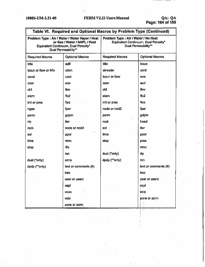
10086-UM-2.21-00 FEHM V2.21 Users Manual QA: QAPage: 164 of 189
Table VI. Required and Optional Macros by Problem Type (Continued)
Problem Type: Air I Water I Water Vapor / Heat Problem Type: Air I Water I No Heator Gas I Water / NAPL / Heat Equivalent Continuum, Dual Porosity*
Equivalent Continuum, Dual Porosity* Dual Permeability"*Dual Permeability**
Required Macros Optional Macros Required Macros Optional Macros
title
boun or flow or hflx
cond
coor
ctrl
elem
hit or pres
ngas
perm
rip
rock
sol
time
stop
dual (*only)
dpdp (**only)
adif
cden
cont
eos
finv
flo2
fixo
fper
gdpm
iter
node or nod2
ppor
renu
rflx
rxn
szna
text or comments (#)
trac
user or userc
vapl
vcon
velo
zone or zonn
title
airwater
boun or flow
coor
ctrl
elem
init or pres
node or nod2
perm
rock
sol
time
stop
dual (*only)
dpdp (**only)
bous
cont
eos
exrl
finv
flo2
fixo
fper
gdpm
head
iter
ppor
pres
renu
rip
rxn
text or comments (#)
trac
user or userc
valpl
velo
zone or zonn

10086-UM-2.21-0D FEHM V2.21 Users Manual QA: QAPage: 165 of 189
9.2 Code ExecutionTo run FEHM, the program executable file name is entered at the system prompt:
<PROMPT> xfehmv2.21
Note that executable names may vary depending on the system being used.
The I/O file Information is provided to the code from an input control file or theterminal. The default control file name is fehmn.files. If a control file with thedefault name is present in the directory from which the code is being executed, noterminal input is required. If the default control file is not present, input promptsare written to the screen. A short description of the I/O files used by FEHMprecedes the initial prompt. The following assumes the default control file was notfound In the execution directory (for this example /home/fehm/heat2d).
After the command xfehm_v2.21 Is given, the code queries the user regarding theInput files, as follows:
Enter name for iocntl -- default file name: not using
[(name/na or not using), RETURN = DEFAULT]
This query asks for a control file name. If a control file name is entered no furtherterminal input is required. Figure 3 shows the control file that would produce thesame results as the terminal responses discussed below and illustrated in Fig. 4.
Ihome/fehm/heat2d/inputlheat2d.inIhome/fehm/heat2d/inputlheat2d.in/home/fehm/heat2d/inputlheat2d.in/home/fehmlheat2d/outputlheat2d.out
/home/fehm/heat2d/outputlheat2d.finIhome/fehm/heat2d/outputlheat2d.his
Ihome/fehmlheat2d/outputlheat2d.chksome0
Figure 3. Input control file for heat conduction example.
Files that are not needed for output can be represented 'ith a blank line. If namesare not provided for the write file and/or the data check'file,:the code Will use thefollowing defaults: fehmn.fin and fehmn.chk. Following the file names is the flagthat controls terminal output. The last line of the file Is the user subroutinenumber. Omitting these values results in no terminal output and no usersubroutine call. For now, we assume a carriage return <Icr>ý is entered and acontrol file is not being used. The following query will appear
Enter name for inpt -- default file name: fehmn.dat 1
[(name/na or not using), RETURN = DEFAULT]

10086-UM-2.21-00 FEHM V2.21 Users Manual QA: QAPage: 166 of 189
This query asks for an input file name. If a <cr> is given, the default fehmn.dat isused for the input file. We shall assume that the input file name entered is
input/heat2d.in
Note that a subdirectory containing the file is also given. If the file did not exist,the code would repeat the prompt for an input file. Next the code would query todetermine if the prefix of the input file name (the portion of the name precedingthe final '." or first space) should be used for code generated file names.
Do you want all file names of the form input/heat2d.* ? [(y/n), RETURN = y]Note: If "y" incoor and inzone will equal inpt
A <cr> will produce files with identical prefixes, including the subdirectory. If theresponse is negative, the code will query for the names of all required files.Assume we enter "n".
Enter name for incoor -- default file name: input/heat2d.in
[(name/na or not using), RETURN = DEFAULT]
(See Fig. 4 for the remaining file name queries.)
Next a query for terminal output appears.
tty output -- show all reference nodes, selected reference nodes, or none:[(all/some/none), RETURN = none]
An "all" reply prints out the primary node information to the terminal at everytime step. A *some" reply prints a selected subset of the node information. A replyof "none" suppresses all tty output with the exception of error messages printed ifcode execution is terminated abnormally or when maximum number of iterationsare exceeded. Assume we enter *some'.
The next query concerns the subroutine USER. This subroutine is used for specialpurposes and is not available to the general user.
user subroutine number (provided to subroutine USER before every time step):[RETURN = none]
Assume a <cr> is entered.
The code will then print a summary of the I/O files to be used.
The final query regards the acceptance of the file set just created. A "yes" replydenotes that the user has accepted the file set and the code proceeds withcalculations. A "no" reply starts the query sequence again so I/O file names may bereentered or modified. A"stop" reply stops the current computer job.
If data is OK enter yes to continue, no to restart terminal input,or stop to end program: [(yes/no/stop), RETURN = yes]
Screen output for this example execution using terminal input and a previousversion of the code is shown in Fig. 4. The only difference in the output is that thecode version identifier and date are updated for the current version. Userresponses are shown in italics. ý

10086-UM-2.21-00 FEHM V2.21 Users Manual QA: QAPage: 167 of 189
<PROMPT> xfehm v2.21sun
version FEHM V2.21sun' 03-09-15 QA:QA
Default names for I/O files
control fileinput filegeometry data filezone data fileoutput fileread file (if it exists)write file (if it exists)history plot filetracer history plot filecontour plot filedual or dpdp contour plot filestiffness matrix data read/write fileinput check file
09/15/2003 11:08:14
: fehmn.files* filen.** filen.*.filen.** filen.out• filen.ini* filen.fin* filen.his* filen.trc* filen.confilen.dpfilen.storfilen.chk
**** where ****"filen.*" may be 100 characters maximum. If a name is not enteredwhen prompted for, a default file name is used. "fehmn.dat" is thedefault used for the input file name.
*** note *,A save file and input check file are always written. If you do notprovide a name for these files, the following defaults will be used:fehmn.fin, fehmn.chk
Enter name for iocntl - default file name: not using
[(name/na or not using), RETURN = DEFAULT]<cr>
Enter name for inpt - default file name: fehmn.dat
[(name/na or not using), RETURN = DEFAULT]input/heat2d.in
Do you want all file names of the form input/heat2d.* ? [(y/n), RETURN = yJ*** Note: If "y" incoor and inzone will equal inpt **n
Enter name for incoor - default file name: input/heat2d.in
[(name/na or not using), RETURN = DEFAULT]<cr>
Figure 4. Terminal query for FEHM example run.

10086-UM-2 .21-00 FEHM V2.21 Users Manual QA: QAPage: 168 of 189
Enter name for inzone - default file name: input/heat2d.in
[(name/na or not using), RETURN = DEFAULT]<cr>
Enter name for iout - default file name: input/heat2d.out
[(name/na or not using), RETURN = DEFAULT]output1heat2d.out
Enter name for iread - default file name: input/heat2d.ini
[(name/na or not using), RETURN = DEFAULT]na
Enter name for isave - default file name: input/heat2d.fin
[(name/na or not using), RETURN = DEFAULT]output/heat2d.fin
Enter name for ishis - default file name: input/heat2d.his
[(name/na or not using), RETURN = DEFAULT]output/heat2d.his
Enter name for istrc - default file name: input/heat2d.trc
[(name/na or not using), RETURN = DEFAULT]na
Enter name for iscon - default file name: inputlheat2d.con
[(name/na or not using), RETURN = DEFAULT]na
Enter name for isconI - default file name: inputlheat2d.dp
[(name/na or not using), RETURN = DEFAULT]na
Enter name for isstor - default file name: input/heat2d.stor[(name/na or not using), RETURN = DEFAULT]na
Enter name for ischk - default file name: input/heat2d.chk
[(name/na or not using), RETURN = DEFAULT]output/heat2d.chk
Figure 4. Terminal query for FEHM example run. (Continued)

10086-UM-2.21-0O FEIM V2.21 Users Manual QA: QAPage: 169 of 189
tty output - show all reference nodes, selected reference nodes, or none:[(all/some/none), RETURN = none]some
user subroutine number (provided to subroutine USER before every time step):[RETURN = none]<cr>
First reference output node will be written to tty
File purpose - Variable - Unit number - File name
control
input
geometry
zone
output
initial state
final state
time history
time his.(tr)
contour plot
con plot (dp)
fe coef stor
Input check
- iocntl - 0 - not using
- inpt - 11 - input/heat2d.in
- incoor - 11 - inputlheat2d.in
- inzone - 11 - input/heat2d.in
- lout - 14 - outputlheat2d.out
- iread - 0 -not using
- isave - 16 - output/heat2d.fin
- ishis - 17 - outputlheat2d.his
- istrc - 18 - not using
- iscon -19 - not using
- isconl - 20 - not using
- isstor -21 - not using
- ischk - 22 - output/heat2d.chk
Value provided to subroutine user: not using
If data is OK enter yes to continue, no to restart terminal input,or stop to end program: [(yes/no/stop), RETURN = yes]<cr>
Figure 4. Terminal query for FEHM example run. (Continued)

10086-UM-2.21-00 FEHM V2.21 Users Manual QA: QAPage: 170 of 189
9.3 Heat Conduction in a SquareThis simple 2-D problem is used to illustrate input file construction and basicoutput. Heat conduction in a 1 meter square with an initial temperature,To = 200 *C, is modeled after a surface temperature, T, = 100 *C, is imposed attime, t = 0 (Fig. 5).The input parameters used for the heat conduction problem aredefined in Table VII.The finite element mesh for this problem. is shown in Fig. 6.Only a quarter of the square needs to be modeled because of problem symmetry.
Table VII. Input Parameters for the 2-D Heat Conduction Problem
Parameter Symbol Value
Rock thermal conductivity, Kr 2.7 .
Rock density Pr 2700 kg/m3
Rock specific heat Cr 1000 kg--K
Width a 0.5 m
Length b 0.5 m
Initial temperature TO 200 01C
Surface temperature 100 0iCfor all x, y = 0.5 m
Rock thermal diffusivity Kcr
PrCr
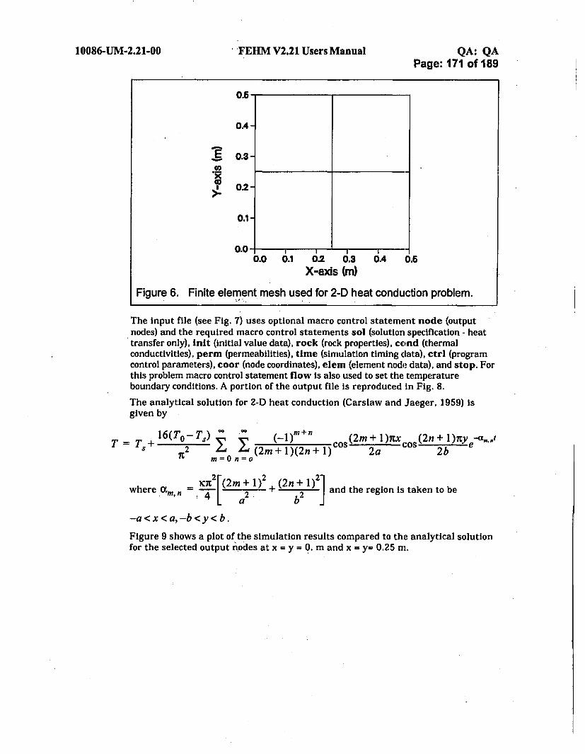
10086-UM-2.21-00 0FEHM V2.21 Users Manual QA: QAPage: 171 of 189
0.5
0.4-
S0.3-
* 02-
0.1-
0.0" , I I0.0 0.1 0.2 0.3 0.4 0.5
X-axis Wm)
Figure 6. Finite element mesh used for 2-D heat conduction problem.
The input file (see Fig. 7) uses optional macro control statement node (outputnodes) and the required macro control statements sol (solution specification - heattransfer only), init (initial value data), rock (rock properties), cond (thermalconductivities), perm (permeabilitles), time (simulation timing data), ctrl (programcontrol parameters), coon (node coordinates), elem (element node data), and stop. Forthis problem macro control statement flow is also used to set the temperatureboundary conditions. A portion of the output file Is reproduced in Fig. 8.
The analytical solution for 2-D heat conduction (Carslaw and Jaeger, 1959) isgiven by
T = Ts+16(TO 2Ts)0
R m=O
(-)m+n (2m + 1)nx (2n + l)1Ye.-am.,t
(2m+ 1)(2n + 52Cos 2a 2bn=o
where am, nME [ + b2+ 2 and the region is taken to be
-a < x < a, -b <y < b.
Figure 9 shows a plot of the simulation results compared to the analytical solutionfor the selected output nodes at x = y = 0. m and x = y= 0.25 m.

10086-UM-2.21-0O FEHM V2.21 Users Manual QA: QAPage: 172 of 189
***** 2-D Heat Conduction Model (2X2 rectangles) *****
node27 5
sol-1 -1
init
10. 0. 200. 0.rock
1 9 1 2700. 10(
0. 200. 0. 0.
)0. 0.
cond1 9 1
perm1 9 1
flow1 3 13 9 3
time0.005 4.
2.7e-00 2.7e-00 2.7e-00
1.e-30 1.e-30 1.e-30
10.00 -100.0010.00 -100.00
00 lOOO 10
1.e031 .e03
1994 02
ctri40 1.e-041 9 1
081
1.0 0.0 1.010 1.0 0.00005 0.0051 0
coor Feb 23, 1994 11:39:4091 0. 0.50 0.2 0.25 0.50 0.3 0.50 0.50 0.4 0. 0.25 0.5 0.25 0.25 0.6 0.50 0.25 0.7 0. 0. 0.8 0.25 0. 0.9 0.50 0. 0.
elem41234
stop
44578
5689
2356
1245
Figure 7. FEHM input file for heat conduction example (heat2d.in).

10086-UM-2.21-OO FEHM V2.21 Users Manual QA: QAPage: 173 of 189
FEHM V2.10 00-06-28 08/07/2000 13:25:08
* 2-D Heat Conduction Model *****
File purpose - Variable - Unit number - File name
control
input
geometry
zone
output
initial state
final state
time history
time his.(tr)
contour plot
con plot (dp)
fe coef stor
- iocntl - 0 - not using
- inpt - 11 - heat2d.in
- Incoor - 11 - heat2d.in
- inzone - 11 - heat2d.in
- lout - 14 - heat2d.out
- iread - 0 - not using
- isave - 16 - fehmn.fin
- ishis - 17 - heat2d.his
- istrc - 0 - not using
- iscon - 0 - not using
- isconl - 0 - not using
- isstor - 0 - not using
input check - ischk - 22 - fehmn.chk
Value provided to subroutine user: not using
input title : coor incoor = 11input title : elem incoor = 11input title : stop * incoor = 11input title : node **** inpt = 11input title : sol inpt = 11input title : init inpt = 11 **
* input title : rock **** inpt = 11input title : cond inpt = 11input title : perm inpt = 11input title : flow * inpt = 11input title : time * inpt = 11
* input title : ctrl inpt = 11input title : stop * inpt = 11
BC to BC connection(s) found(now set=0.0)BC to BC connection(s) found(now set=0.0)
Figure 8. FEHM output from the 2-D heat conduction example.

10086-UM-2.21-OO FEHM V2.21 Users Manual QA: QAPage: 174 of 189
pressures and temperatures set by gradients>>>reading nop from file nop.temp.....>>>reading nop was succesful .....
storage needed for ncon 43 available 43storage needed for nop 43 available 46storage needed for a matrix 33 available 33storage needed for b matrix 33 available 46storage needed for gmres 81 available 81storage available for b matrix resized to 33<<<<<<
time for reading input, forming coefficients 0.204E-01
analysis of input data on file fehmn.chk
Time Step 1
Timing InformationYears Days Step Size (Days)
0.136893E-04 0.500000E-02 0.500000E-02Cpu Sec for Time Step = 0.8081E-03 Current Total = 0.2650E-02
Equation PerformanceNumber of N-R Iterations: 1Avg # of Linear Equation Solver Iterations: 3.0Number of Active Nodes: 9.Total Number of Newton-Raphson Iterations: 1,s
Largest ResidualsEQ1 R= 0.1660E-07 node= 5 x=0.2500 y=0.2500
Node Equation 1 Residual Equation 2 Residual7 0.11 1444E-07 0.185894E-015 0.165983E-07 0.135450E+01
olver: 3
z= 1.000
k(MJ/s)0.0.
Nodal Information (Water)
Node75
source/sinkp(MPa) e(MJ)10.000 0.0010.000 0.00
I sat0.0000.000
temp(c)199.981198.645
source/sinl(kg/s)0.
5 0.
Global Mass & Energy BalancesTotal mass In system at this time: 0.OOOOOOE+00 kgTotal mass of steam in system at this time: 0.OOOOOOE+00 kgTotal enthalpy in system at this time: 0.105123E+03 MJ
Water discharge this time step:Water input this time step:Total water discharge:Total water input:
0.OOOOOOE+00 kg (0.OOOOOOE+00 kg/s)0.OOOOOOE+00 kg (0.OOOOOOE+00 kg/s)0.OOOOOOE+00 kg (0.OOOOOOE+00 kg/s)0.000000E+00 kg (0.OOOOOOE+00 kg/s)
Figure 8. FEHM output from the 2-D heat conduction example. (Continued)

10086-UM-2.21-OO FEHM V2.21 Users Manual QA: QAPage: 175 of 189
Enthalpy discharge this time step:Enthalpy input this time step:Total enthalpy discharge:Total enthalpy input:
0.297800E+02 MJ (0.689352E-01 MJ/s)O.OOOOOOE+00 MJ (0.000000E+00 MJ/s)0.297800E+02 MJ (0.689352E-01 MJ/s)0.297800E+02 MJ (0.689352E-01 MJ/s)
Net kg water discharge (total out-total in): 0.OOOOOOE+00Net MJ discharge (total out-total in): 0.000000E+00Conservation Errors: 0.000000E+00 (mass), -0.100326E+01 (energy)
Time Step 11
Time Step 801
Timing InformationYears Days Step Size (Days)
0.109515E-01 0.400005E+01 0.500000E-04Cpu Sec for Time Step = 0. Current Total = 4.533
Equation PerformanceNumber of N-R Iterations: 1Avg # of Linear Equation Solver Iterations: 2.0Number of Active Nodes: 9.Total Number of Newton-Raphson Iterations: 801 , Solver:
Largest ResidualsEQ1 R= 0.9774E-13 node= 7 x= 0.000 y= 0.000 z= 1.000
Node Equation 1 Residual Equation 2 Residual7 0.977369E-13 0.186062E-045 0.621566E-13 0.930309E-05
2402
Nodal Information (Water)
Node75
source/sinkp(MPa) e(MJ)10.000 0.0010.000 0.00
I sat0.0000.000
source/sinktemp(c) (kg/s)100.230 0.100.115 0.
(MJ/s)0.0.
Global Mass & Energy BalancesTotal mass in system at this time: 0.OOOOOOE+00 kgTotal mass of steam in system at this time: 0.OOOOOOE+00 kgTotal enthalpy in system at this time: 0.675565E+02 MJ
Water discharge this time step:Water input this time step:Total water discharge:Total water input:
Enthalpy discharge this time step:Enthalpy input this time step:
0.OOOOOOE+00 kg (0.OOOOOOE+00 kg/s)0.OOOOOOE+00 kg (0.OOOOOOE+00 kg/s)0.OOOOOOE+00 kg (0.OOOOOOE+00 kg/s)0.OOOOOOE+00 kg (0.OOOOOOE+00 kg/s)
0.455636E-05 MJ (0.105471E-05 MJIs)0.OOOOOOE+00 MJ (0.OOOOOOE+00 MJ/s)
Figure 8. FEHM output from the 2-D heat conduction example. (Continued)
;. rý
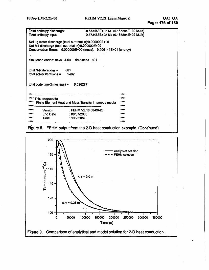
10086-UM-2.21-OO FEHM V2.21 Users Manual QA: QAPage: 176 of 189
Total enthalpy discharge:Total enthalpy input:
0.673463E+02 MJ (0.155894E+02 MJ/s)0.673463E+02 MJ (0.155894E+02 MJ/s)
Net kg water discharge (total out-total in):O.000000E+00Net MJ discharge (total out-total in):0.OOOOOOE+00Conservation Errors: O.000000E+00 (mass), -0.100144E+01 (energy)
simulation ended: days 4.00 timesteps 801
total N-R iterations =total solver iterations =
8012402
total code time(timesteps) = 0.526277
**** This program for* Finite Element Heat and Mass Transfer in porous media
VersionEnd DateTime
FEHM V2.10 00-06-2808/07/200013:25:08-
Figure 8. FEHM output from the 2-D heat conduction example. (Continued)
200-
180 -
0 L55"-" 160-
x, y0.0m®S
4)S0. 140E0)
120x, y 0.25 m
1000 50000 100000 150000 200
Time (s)
000 250000 300000 350000
Figure 9. Comparison of analytical and model solution for 2-D heat conduction.

10086-UM-2.21-00 FEHM V2.21 Users Manual QA: QAPage: 177 of 189
9.4 DOE Code Comparison Project, Problem 5, Case A
This problem involves multiphase flow in a 2-D horizontal reservoir. The problemis characterized by a moving two-phase region, i.e., the fluid produced at theproduction well is replaced by cold water recharge over one of the outerboundaries. The problem parameters are given in Table VIII and the geometry andboundary conditions are shown in Fig. 10. Of particular note are the variableinitial temperature field, provided to the code through a read file (see Section 5.6on page 18), and the prescribed pressure and temperature on the right boundary.Apartial listing of the input file is provided in Fig. 11. In addition to the requiredmacros, macro flow is used to specify the pressure and temperature boundarycondition and the production flow rate. Macro rip is used to set the residual liquidand gas saturations.
Table VIII.Input Parameters for the DOE Code ComparisonProject Problem
Parameter Symbol Value
Reservoir permeability k 2.5 x 10⁻¹⁴ m2
Reservoir porosity 4 0.35
Rock thermal conductivity icr 1 mim.K
Rock density Pr 2563 kg/m3
Rock specific heat Cr 1010 kgK
Reservoir length x 300 m
Reservoir thickness y 200 m
Liquid residual saturation SIr 0.3
Gas residual saturation Sgr 0.1
Reservoir discharge qm 0.05 _gm-s
Initial Pressure PO 3.6 MPa
Production well coordinates: x = 62.5 m, y = 62.5 m
Observation well coordinates: x = 162.5 m, y = 137.5 m
Initial temperature distribution (Tin 0C, r in m):
240 r:5 001(r 100 (r-+8 00'4-(x,y,O) 240-160 +80 2 100<r<300
160 r > 300
where r = 2
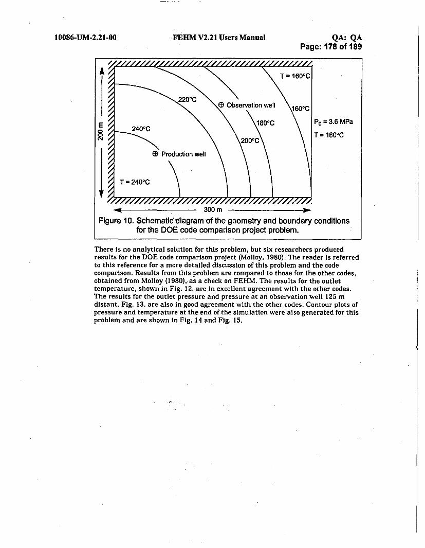
10086-UM-2.21-00 FEEM V2.21 Users Manual QA: QAPage: 178 of 189
There is no analytical solution for this problem, but six researchers producedresults for the DOE code comparison project (Molloy, 1980). The reader is referredto this reference for a more detailed discussion of this problem and the codecomparison. Results from this problem are compared to those for the other codes,obtained from Molloy (1980), as a check on FEHM. The results for the outlettemperature, shown in Fig. 12, are in excellent agreement with the other codes.The results for the outlet pressure and pressure at an observation well 125 mdistant, Fig. 13, are also in good agreement with the other codes. Contour plots ofpressure and temperature at the end of the simulation were also generated for thisproblem and are shown in Fig. 14 and Fig. 15.

10086-UM-2.21-00 FEHM V2.21 Users Manual QA: QAPage: 179 of 189
*** DOE Code Comparison Project, Problem 5, Case A ***
node2
50 88sol
1 1
init3.6 0. 240. 0. 0. 240. 0. 0.
rip2 0.3 0.1 0.0 0.0
1 140 1 1
rock1 140 1 2563. 1010. 0.35
cond1 140 1 1.00e-00 1.00e-00 1.00e-00
perm1 140 1 2.5e-14 2.5e-14 0.e-00
flow88 88 1 0.050 -25.00 0.14 140 14 3.600 -160.00 1.
time30.0 3650. 10000 1000 1994 03
ctrl40 1.e-07 08
1 140 1 1
1.0 0.0 1.040 1.2 0.1 60.
1 0coor
140
elem4 117
stop
Figure 11. FEHM input file for DOE problem.

10086-UM-2.21-00 FEHM V2.21 Users Manual QA: QAPage: 180 of 189
240 - 24-- FEHM
20 Code I235 0 Code 2
-I+ Code 3
230- X Code 40 Code 5
El E Code 6o225-
220-
E 215-
210-
205 -
200 ' ' '
0 2 4 6 8 10
Time (years)
Figure 12. Comparison of FEHM production well temperatures with resultsfrom other codes.
0.1 0 Code1 X Code4
0.2 •• P-• []0 Code 2 0] Code 5
. 13+ Code 3 El Code 6
0.2M 0.3 -D '3 0l El eM e 0 O
Observation well0.4 -
0.5 )0
.~ ~ x >v"0:< +00.6 ;
Production well
0.7 _'-T --- - - -
0 2 4 6 8 10
Time (years)
Figure 13. Comparison of FEHM production and observation well pressuredrops with results from other codes.

10086-UM-2.21-OO FEHM V2.21 Users Manual QA: QAPage: 181 of 189
E-
.5
150
100
50
Reservoir length (mn)
Figure 14. Contour plot of pressure at ten years for the DOE problem.

10086-UM-2.21-00 FEHM V2.21 Users Manual QA: QAPage: 182 of 189
9.5 Reactive Transport ExampleThis one-dimensional example demonstrates the use of the reactive transportmodule of FEHM. The application of this simulation is the transport of cobalt (Co)in groundwater. Radioactive cobalt is present in the subsurface at several DOEsites. Although its presence as a divalent cation implies that it should sorbstrongly to most soils, its migration rate has been shown to be greater thanexpected due to complexation with EDTA, a decontaminating agent also found inthe subsurface of these sites. Much experimental work has gone into studying thetransport of Co as CoEDTA, a much less strongly sorbed species. The chemicalreactions and equilibrium or rate constants used to perform this simulation are:
CoEDTA(,q) <* Co(aq) + EDTA(aq); Keq = 10-8 kg/mol (16)
27Fe(aq) +EDTA(aq) , FeEDTA(aq) ; Keq 6.31x10 kg/mol (17)
Co(aq) 4* CO(s) ; kf = 2.78x10⁻⁴ s-1, kr = 5.48x10⁻⁵ s- 1 (18)
CoEDTA(aq) '=* CoEDTA( ; kf = 2.78xl0- S-1,
kr = 5.21x10⁻⁴ s-1 (19)
FeEDTA(aq) t-* FeEDTA() ; kf = 2.78x10- s-1
kr = 6.5x10⁻⁴ s- 1 (20)
CoEDTA(s) + Fe(OH)3(s) => Co(s) + FeEDTA(,);
kf 3.5x10- s-1 (21)
Thus the transport system consists of 8 species and six reactions, with reactionsspecified as either equilibrium or kinetically controlled. Fe(OH) 3 is so prevalent inthe sand that its concentration is assumed to be constant. In addition, it does notact as a true species in the simulation. A list of relevant input parameters andconditions for the simulation are given in Table IX. Figure 16 illustrates thetransport problem. The flow system is represented by a one-dimensional flow pathof 202 nodes (101 x 2). A partial listing of the input file is provided in Fig. 17.
FEHM results for this problem are compared to those of PDREACT (Valocchi et
al., 1994), a two-dimensional, Isothermal, saturated-zone flow and transport codein Figs. 18 and 19.

10086-UM-2.21-OO FEHM V2.21 Users Manual QA: QAPage: 183 of 189
u = 1 n/hr
Cin, Co(aq)
Cin, Fe(aq)
Cin, EDTA(aq)
Column filled with Fe(OH)3 SandP= 1 MPa
P0 = 1 MPa
Figure 16. Schematic drawing of the geometry and boundary conditionsfor the cobalt transport problem.
Table IX. Input Parameters for the Reactive Transport TestProblem
Parameter Symbol Value
Reactor Length L 10 m
Node spacing Al 0.1 m
Fluid Density Pf 1000 kg/m3
Bulk Rock Density Pb 1500 kg/m3
Porosity 0.4
Pore Water Velocity u 1 m/hr
Dispersivity a 0.05 m
Time step (tracer) At 0.09 - 360 s
Total elapsed time t 7.25 days
Pressure PO 1.0 MPa
Co Inlet Concentration Cin, CO 3.1623x10⁻⁵ M
Fe Inlet Concentration C'in, Fe 0 M
EDTA Inlet Concentration Cin, EDTA 3.1623x10⁻⁵ M
Boundary conditions: At I = 0 U =Atl=1 P=
*Flow rate q = upfO/2 nodes 0.05556 kg/s
1 m/hr1 MPa

10086-UM-2.21-00 FEHM V2.21 Users Manual QA: QAPage: 184 of 189
COMPARE FEHMN and PDREACT: Linear Sorption w/ Surface Exchangecond1202 12.7 2.7 2.7
ctrl50 le-6 81 202 1 2
100.525 2. 1.e-6 1.e-110flow1 202 101 -0.05556 -25 0101202 101 1.-25-1
hit1.25 25 0 1000 25 0 0node1202perm1 202 1 5.0e-13 5.0e-30 5.0e-30
rock1202 1 1500 1000 0.4
sol1 -1time1.e-6 7.25 1000 10 92 11
# solute 1: Total Cobalt Concentration# solute 2: Total Iron Concentration# solute 3: Total EDTA Concentration# solute 4: CoEDTA adsorbed concentration# solute 5: Co adsorbed concentration# solute 6: FeEDTA adsofrbed concentrationtrac0.0 1.0 1.e-6 0.51. 2000 1.0 20005 5.0 1.e-6 4.1667e-3611 0. 0. 1. 1.e-9.05 1.e-34 1.e-34
1 202 11
1 202 1 0.
1202 101 3.1623e-5 1.0 4.16667
Figure 17. FEHM input file for reactive transport problem.

10086-UM-2.21-OO FEHM V2.21 Users Manual QA: QAPage: 185 of 189
11 0. 0. 1. 1.e-9.05 1.e-34 1.e-34
1 202 11
1 202 1 0.
1 202 101 1.e-13 1.0 4.16667
11 0. 0. 1. 1.e-9.05 1.e-34 1.e-34
1 202 11
1 202 1 0.
1 202 101 3.1623e-5 1.0 4.16667
01 202 1 0.
01 202 1 0.
01 202 1 0.0
rxn** NCPLX, NUMRXN2,4** Coupling of the aqueous components (dRi/dUj)2101010** IDCPNT(IC),CPNTNAM(IC),IFXCONC(IC),CPNTPRT(IC) (comp,name,cond.; NCPNTrows)1 Cobalt[aq] 0 0 1.e-92 Iron[aq] 0 0 1.e-93 EDTA[aq] 0 0 1.e-9** IDCPLX(IX), CPLXNAM(IX),CPLXPRT(IX) (ID # and name of complex, NCPLX rows)101 Co-EDTA[aq] 0102 Fe-EDTA[aq] 0** IDIMM(IM), IMMNAM(IM),IMMPRT(IM)(ID # and name of immobile spec, NIMM rows)1 Co-EDTA[s] 02 Fe-EDTA[s] 03 Cobalt[s] 0** IDVAP(IV), VAPNAM(IM), VAPPRT(IV) (ID # and name of vapor spec, NVAP rows)** Skip nodes0
Figure 17. FEHM input file for reactive transport problem (Continued).

10086-UM-2.21-00 FEHM V2.21 Users Manual QA: QAPage: 186 of 189
** RSDMAX1.0e-10**** Chemical reaction information for equilibrium reactions ..** LOGKEQ (=0 if stability constants are given as K, =1 if given as log(K))
0** CKEQ(IX) ,HEQ(IX) (Stability constants and Enthaplys, NCPLX rows)1.0e+18 06.31e+27 0** STOIC(IX,IC) (Stoichiometric coeff: NCPLX rows, NCPNT columns)1.0 0.0 1.00.0 1.0 1.0** LINEAR KINETIC REACTION (type 1) **
1** Where does the reaction take place? **
100
** Aqueous Component/Complex #, Solid Component #
101 1** Distribution coeffienct (kg water/ kg rock) **
0.533** Mass transfer coefficient (1/hr) **
1.0LINEAR KINETIC REACTION (type 1) **
1** Where does the reaction take place?100
** Aqueous Component/Complex #, Solid Component #1 3
** Distribution coeffienct (kg rock/ kg water) **
5.07** Mass transfer coefficient (1/hr) **
1.0** LINEAR KINETIC REACTION (type 1) **
1** Where does the reaction take place? **
100
** Aqueous Component/Complex #, Solid Component #102 2
** Distribution coeffienct (kg rock/ kg water) **
0.427** Mass transfer coefficient (1/hr)
1.0** GENERAL EXCHANGE REACTION (type 3)
3** Where does the reaction take place? **
100
** # of solid, liquid and vapor species
300
Figure 17. FEHM input file for reactive transport problem (Continued).

10086-UM-2.21-00 FEHM V2.21 Users Manual QA: QAPage: 187 of 189
** forward and reverse rate constants (1/hr) **
1.26e-2 0** Solid Species in reaction **
1 2 3** Stoichiometry **
1.0 -1.0 -1.0coor n/a
2021 0.00000 1.00000 0.000002 0.10000 1.00000 0.000003 0.20000 1.00000 0.00000
200 9.80000 0.00000 0.00000201 9.90000 0.00000 0.00000202 10.00000 0.00000 0.00000
elem4 1001 102 103 2 12 103 104 3 23 104 105 4 3
98 199 200 99 9899 200 201 100 99100 201 202 101 100
stop
Figure 17. FEHM input file for reactive transport problem (Continued).

10086-UM-2.21-OO FEHM V2.21 Users Manual QA: QAPage: 188 of 189
0.025 -
o CoEDTA (aq) -- FEHMT" " 0 PDREACT
'0 0.020-
7 0.015C
0L)0.0 FeEDTA (a)
U) 0.0105
Co (aq)
0.000*0 25 50 75 100 125 150
Time (hrs)
Figure 18. Comparison of FEHM and PDREACT for the breakthroughcurves of aqueous species.
0.0150-- FEHM
0 PDREACT Co (S)
" 0.0125 CoEDTA (s)
2
0.01000
0.0075
• 0.0050
5 0.0025 -FeEDTA (s)
0.0000' '
0 25 50 75 100 125 150
Time (hrs)
Figure 19. Comparison of FEHM and PDREACT for the exitconcentration versus time for solid species.

10086-UM-2.21-00 FEHM V2.21 Users Manual QA: QAPage: 189 of 189
10.0 USER SUPPORTLicensing and installation support can be received from:
Zora [email protected]
Technical support can be received from:
George [email protected]
Bruce [email protected]


![Aristotle University of Thessalonikiusers.auth.gr/users/0/2/066520/public_html/Journal Papers/Planning... · útil para um planejamento orientado da cobertura 3]; a média mais forte](https://img.pdfslide.us/doc/110x75/5fe3d850b390bb0b1a7d3874/aristotle-university-of-papersplanning-til-para-um-planejamento-orientado.jpg)