Software Safety

Lecture 8: System Reliability

Elena Troubitsyna Anton Tarasyuk

Abo Akademi University

System Dependability

A. Avizienis, J.-C. Laprie and B. Randell:Dependability and its Threats (2004):

Dependability is the ability of a system to deliver a service thatcan be justifiably trusted or, alternatively, as the ability of a systemto avoid service failures that are more frequent or more severe thanis acceptable

Dependability attributes: reliability, availability, maintainability,safety, confidentiality, integrity

Reliability Definition

Reliability : the ability of a system to deliver correct service undergiven conditions for a specified period of time

Reliability is generally measured by the probability that a system(or system component) S can perform a required function undergiven conditions for the time interval [0, t]:

R(t) = P {S not failed over time [0, t]}

More Definitions

Failure rate (or failure intensity): the number of failures per timeunit (hour, second, ...) or per natural unit (transaction, run, ...)

• can be considered as an alternative way of expressing reliability

Availability : the ability of a system to be in a state to delivercorrect service under given conditions at a specified instant of time

• usually measured by the average (over time) probability that asystem is operational in a specified environment

Maintainability : the ability of a system to be restored to a state inwhich it can deliver correct service

• usually measured by the probability that maintenance of thesystem will restore it within a given time period

Safety-critical Systems

• Pervasive use of computer-based systems in many criticalinfrastructures

• flight/traffic control, driverless trains/cars operation, nuclearplant monitoring, robotic surgery, military applications, etc.

• Extremely high reliability requirements for safety-criticalsystems

• avionics domain example: failure rate ≤ 10−9 failures per hour,i.e., more than a hundred years of operation withoutencountering a failure

Hardware vs. Software

• Hardware for safety-critical systems is very reliable and itsreliability is being improved

• Software is not as reliable as hardware, however, its role insafety-critical systems increases

• The division between hardware and software reliability issomewhat artificial [J. D. Musa, 2004]

• Many concepts of software reliability engineering are adaptedfrom the mature and successful techniques of hardwarereliability

Hardware Failures

The system is said to have a failure when its actual behaviourdeviates from the intended one specified in design documents

Underlying faults: the largest part of hardware failures caused byphysical wear-out or physical defect of a component

• transient faults: the faults that may occur and then disappear aftersome period of time

• permanent faults: the faults that remain in the system until theyare repaired

• intermittent faults: the reoccurring transient faults

Failure Rate

The failure rate of a system (or system component) is the meannumber of failures within a given period of time

The failure rate is a random variable (gives us the probability thata system, which has been operating over time t, fails over the nexttime unit)

The failure rate of a component normally varies with time: λ(t)

Failure Rate (ctd.)

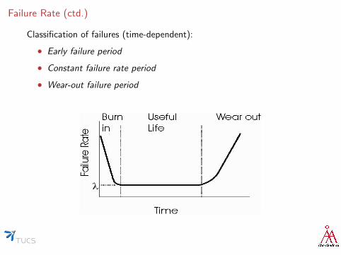
Classification of failures (time-dependent):

• Early failure period

• Constant failure rate period

• Wear-out failure period

Failure Rate (ctd.)

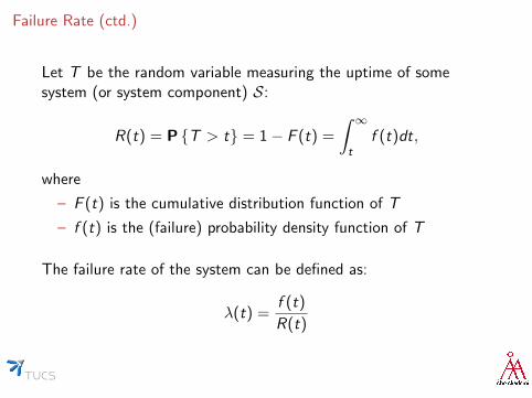
Let T be the random variable measuring the uptime of somesystem (or system component) S:

R(t) = P {T > t} = 1− F (t) =

∫ ∞t

f (t)dt,

where

– F (t) is the cumulative distribution function of T

– f (t) is the (failure) probability density function of T

The failure rate of the system can be defined as:

λ(t) =f (t)

R(t)

Most Important Distributions

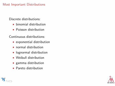
Discrete distributions:

• binomial distribution

• Poisson distribution

Continuous distributions:

• exponential distribution

• normal distribution

• lognormal distribution

• Weibull distribution

• gamma distribution

• Pareto distribution

Repair Rate

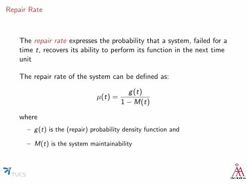
The repair rate expresses the probability that a system, failed for atime t, recovers its ability to perform its function in the next timeunit

The repair rate of the system can be defined as:

µ(t) =g(t)

1−M(t)

where

– g(t) is the (repair) probability density function and

– M(t) is the system maintainability

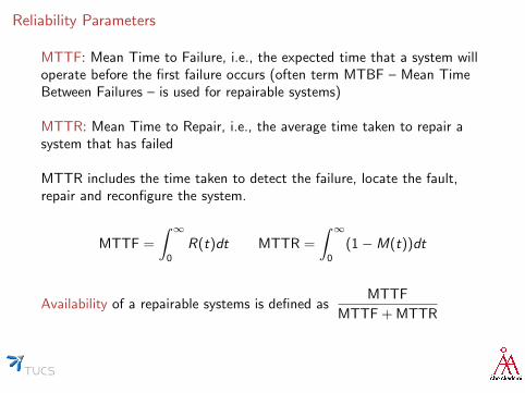
Reliability Parameters

MTTF: Mean Time to Failure, i.e., the expected time that a system willoperate before the first failure occurs (often term MTBF – Mean TimeBetween Failures – is used for repairable systems)

MTTR: Mean Time to Repair, i.e., the average time taken to repair asystem that has failed

MTTR includes the time taken to detect the failure, locate the fault,repair and reconfigure the system.

MTTF =

∫ ∞0

R(t)dt MTTR =

∫ ∞0

(1−M(t))dt

Availability of a repairable systems is defined asMTTF

MTTF + MTTR

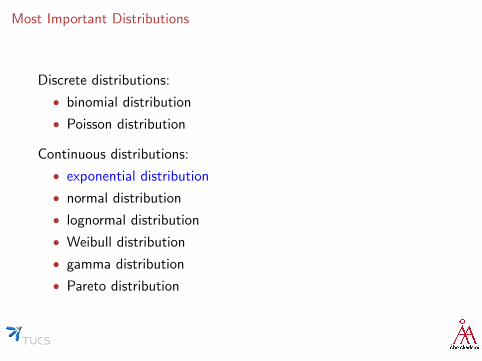
Most Important Distributions

Discrete distributions:

• binomial distribution

• Poisson distribution

Continuous distributions:

• exponential distribution

• normal distribution

• lognormal distribution

• Weibull distribution

• gamma distribution

• Pareto distribution

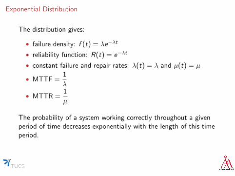
Exponential Distribution

The distribution gives:

• failure density: f (t) = λe−λt

• reliability function: R(t) = e−λt

• constant failure and repair rates: λ(t) = λ and µ(t) = µ

• MTTF =1

λ

• MTTR =1

µ

The probability of a system working correctly throughout a givenperiod of time decreases exponentially with the length of this timeperiod.

Exponential Distribution (cont.)

The exponential distribution is often used in calculations as theyare thus made much simpler

During the useful-life stage, the failure rate is related to thereliability of the component or system by exponential failure law

Describes neither the case of early failures (decreasing failure rate)nor the case of worn-out components (increasing failure rate)

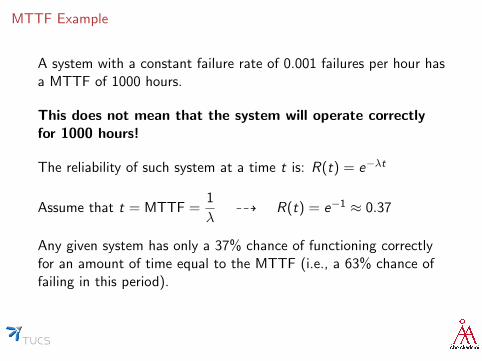
MTTF Example

A system with a constant failure rate of 0.001 failures per hour hasa MTTF of 1000 hours.

This does not mean that the system will operate correctlyfor 1000 hours!

The reliability of such system at a time t is: R(t) = e−λt

Assume that t = MTTF =1

λ99K R(t) = e−1 ≈ 0.37

Any given system has only a 37% chance of functioning correctlyfor an amount of time equal to the MTTF (i.e., a 63% chance offailing in this period).

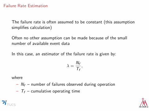
Failure Rate Estimation

The failure rate is often assumed to be constant (this assumptionsimplifies calculation)

Often no other assumption can be made because of the smallnumber of available event data

In this case, an estimator of the failure rate is given by:

λ =Nf

Tf,

where

– Nf – number of failures observed during operation

– Tf – cumulative operating time

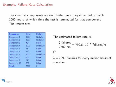
Example: Failure Rate Calculation

Ten identical components are each tested until they either fail or reach

1000 hours, at which time the test is terminated for that component.

The results are:

12 April 2007 8

Failure rate calculation example

� Ten identical components are each tested until they either fail or reach 1000 hours, at which time the test is terminated for that component. The results are:Component Hours Failure

Component 1 1000 No failure

Component 2 1000 No failure

Component 3 467 Failed

Component 4 1000 No failure

Component 5 630 Failed

Component 6 590 Failed

Component 7 1000 No failure

Component 8 285 Failed

Component 9 648 Failed

Component 10 882 Failed

Totals 7502 6

Estimated failure rate is:

or =799.8 failures for every million hours of operation.

The estimated failure rate is:

6 failures

7502 hrs= 799.8 · 10−6 failures/hr

or

λ = 799.8 failures for every million hours of

operation.

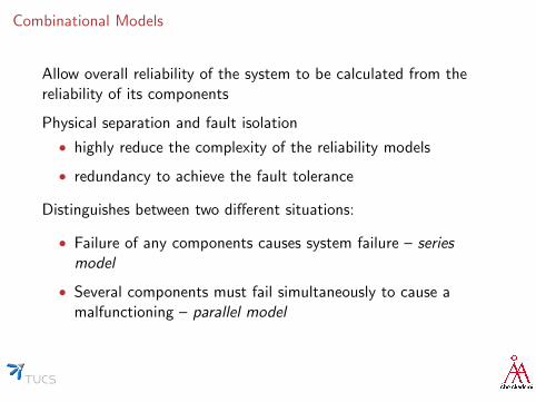
Combinational Models

Allow overall reliability of the system to be calculated from thereliability of its components

Physical separation and fault isolation

• highly reduce the complexity of the reliability models

• redundancy to achieve the fault tolerance

Distinguishes between two different situations:

• Failure of any components causes system failure – seriesmodel

• Several components must fail simultaneously to cause amalfunctioning – parallel model

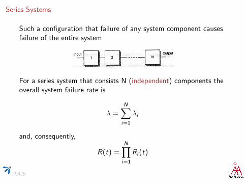
Series Systems

Such a configuration that failure of any system component causesfailure of the entire system

For a series system that consists N (independent) components theoverall system failure rate is

λ =N∑i=1

λi

and, consequently,

R(t) =N∏i=1

Ri (t)

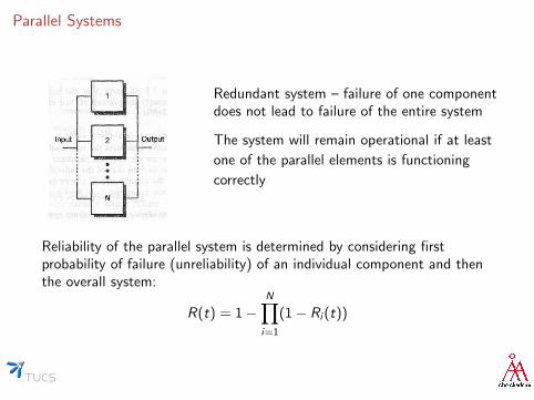
Parallel Systems

Redundant system – failure of one componentdoes not lead to failure of the entire system

The system will remain operational if at least

one of the parallel elements is functioning

correctly

Reliability of the parallel system is determined by considering firstprobability of failure (unreliability) of an individual component and thenthe overall system:

R(t) = 1−N∏i=1

(1− Ri (t))

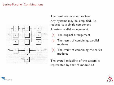
Series-Parallel Combinations

The most common in practice.

Any systems may be simplified, i.e.,reduced to a single component

A series-parallel arrangement:

(a) The original arrangement

(b) The result of combining parallelmodules

(c) The result of combining the seriesmodules

The overall reliability of the system is

represented by that of module 13

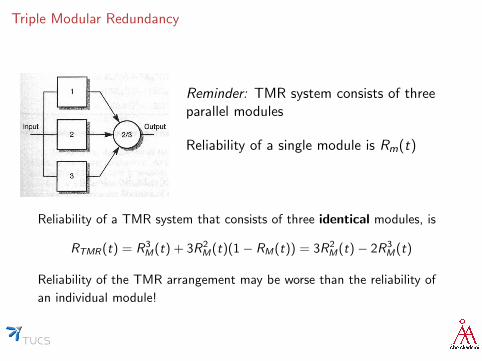
Triple Modular Redundancy

Reminder: TMR system consists of threeparallel modules

Reliability of a single module is Rm(t)

Reliability of a TMR system that consists of three identical modules, is

RTMR(t) = R3M(t) + 3R2

M(t)(1− RM(t)) = 3R2M(t)− 2R3

M(t)

Reliability of the TMR arrangement may be worse than the reliability of

an individual module!

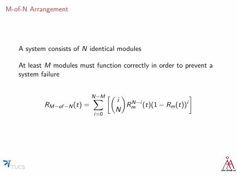
M-of-N Arrangement

A system consists of N identical modules

At least M modules must function correctly in order to prevent asystem failure

RM−of−N(t) =N−M∑i=0

[(i

N

)RN−im (t)(1− Rm(t))i

]

Software Reliability

• Software, in general, logically more complex

• Software failures are design failures

• caused by design faults (have human nature)

• design = all software development steps (from requirements todeployment and maintenance)

• harder to identify, measure and detect

• Software does not wear out

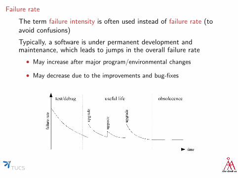
Failure rate

The term failure intensity is often used instead of failure rate (toavoid confusions)

Typically, a software is under permanent development andmaintenance, which leads to jumps in the overall failure rate

• May increase after major program/environmental changes

• May decrease due to the improvements and bug-fixes

Software Reliability (ctd.)

• Software, unlike hardware, can be fault-free (theoretically :))• some formal methods can guarantee the correctness of

software (proof-based verification, model checking, etc.)

• Correctness of software does not ensure its reliability!• software can satisfy the specification document, yet the

specification document itself might already be faulty

• No independence assumption, i.e., copies of software will failtogether

• most hardware fault tolerance mechanisms ineffective forsoftware

• design diversity instead of component redundancy(e.g., N-version programming )

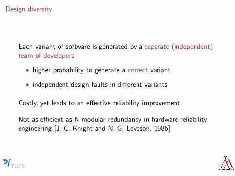
Design diversity

Each variant of software is generated by a separate (independent)team of developers

• higher probability to generate a correct variant

• independent design faults in different variants

Costly, yet leads to an effective reliability improvement

Not as efficient as N-modular redundancy in hardware reliabilityengineering [J. C. Knight and N. G. Leveson, 1986]

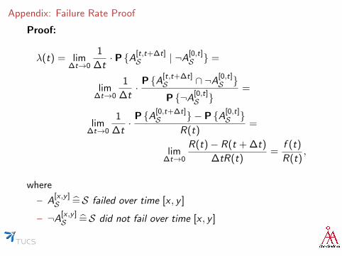
Appendix: Failure Rate Proof

Proof:

λ(t) = lim∆t→0

1

∆t· P {A[t,t+∆t]

S | ¬A[0,t]S } =

lim∆t→0

1

∆t·P {A[t,t+∆t]

S ∩ ¬A[0,t]S }

P {¬A[0,t]S }

=

lim∆t→0

1

∆t·P {A[0,t+∆t]

S } − P {A[0,t]S }

R(t)=

lim∆t→0

R(t)− R(t + ∆t)

∆tR(t)=

f (t)

R(t),

where

– A[x ,y ]S =S failed over time [x , y ]

– ¬A[x ,y ]S =S did not fail over time [x , y ]