Software review – multilevel models in GenStat Sue …bristol.ac.uk/cmm/learning/mmsoftware/reviewgenstat.pdfN:\Amydata\Library\review\reviewgenstat.doc 03/06/03 Software review

$Page 1: Software review – multilevel models in GenStat Sue …bristol.ac.uk/cmm/learning/mmsoftware/reviewgenstat.pdfN:\Amydata\Library\review\reviewgenstat.doc 03/06/03 Software review$
N:\Amydata\Library\review\reviewgenstat.doc 03/06/03

Software review – multilevel models in GenStat

Sue Welham Medical Statistics Unit, LSHTM/Rothamsted Research Ltd.

1. Introduction to the software 1.1 Background GenStat was first developed in the 1960s at Rothamsted Experimental Station for use in design and analysis of agricultural experiments and has been in continuous development since. A REML algorithm for analysis of simple multilevel models was added in 1989, and an interface to the ASREML algorithm using sparse matrix methods and an efficient updating algorithm was achieved in 1995, which also provided a wider range of variance structures for multilevel models. In the 1990s, a Windows interface was added to provide a flexible menu-driven user interface and the graphics facilities have recently been upgraded. Although most areas of statistical application are covered, GenStat’s particular strengths are in its ANOVA algorithm, which analyses balanced multi-level data, and the efficient REML algorithm which analyses multi-level data, allowing for correlated errors at any level of the data. There are also good facilities for GLMs. The major user group is statisticians and scientists working in biological research. 1.2 Software and hardware requirements for the latest version (GenStat 6th Edition, SP 1) • Operating systems: PC Windows (95, 98, 2000, NT or XP), Linux, Unix, details of other

implementations available from VSN International • Online help: Available on PC Windows implementations • Machines supported: details available from VSN International • Memory requirements: 64 Mb minimum • Other requirements: for Windows implementation, Pentium or compatible processor, 80Mb hard

disk space (maximum) 1.3 Data input/output functionality

• Data types that can be imported: Windows implementation: ASCII, Lotus, Minitab, dBase, Excel, SAS, Quattro, SPSS, Paradox, S+, Matlab, Systat, Arcview, Mstat, MapInfo, Stata, Gauss, INSTAT, Epi-info, plus ODBC data retrieval. For other implementations, a wider range of formats is available through the DATALOAD procedure.

• Data types that can be saved: Excel, Lotus, Quattro, dBase, Gauss, SAS, S+, INSTAT, Minitab, ASCII, csv, HTML, RTF, ARCGiS. Also, GenStat spreadsheet can be used to save GenStat data structures, and current session can be saved.

• Output files: GenStat spreadsheet files or the current session can be saved. The output can be saved to a file, as well as a log of commands used, or any text (eg. command) files created during the session. Graphs can be saved in a wide range of formats (including postscript).

• Handling of data input and output: data input can be handled through the command interface by reading ASCII files, or by using menus to load data from a wide range of formats (see above) into the GenStat spreadsheet structure. This allows manipulation of the data (if required) before sending to the server (which makes the data active). Several data sets can be loaded and used together in a single session.

-2-


1.4 Interface features

Within the Windows implementation, the full GenStat command language is available, so that programs can be written and run. There are also menus available for all standard data manipulation and analysis, as well as for many more complex analyses. Where menus are used, the commands generated are logged so that the analysis is repeatable and a full audit trail is available.

2. Standard modelling tools for multilevel analysis 2.1 A brief checklist of facilities for multilevel modelling in GenStat Table 1 provides an overview of the facilities for multilevel models in GenStat. The widest range of facilities is available for models with normal error variables, but there are also several sets of procedures available for fitting multi-level models with non-normal errors.

Table 1. Multilevel models that can be fitted in GenStat Data / model type Estimation

procedures Limitation on levels in data

Allowing covariates

Allowing random slopes

Weighting Fitting variance function

(any level)

Other comments/limitations

Normal response REML No Yes Yes Yes Some* Fast sparse algorithm Binary/Binomial PQL, MQL,

HGLM No Yes Yes for

HGlM No Yes for

HGLM PQL, MQL in GLMM procedure or PQL in IRREML procedure. Separate procedures for HGLMs.

Poisson PQL, MQL, HGLM

No Yes Yes for HGML

No Yes for HGLM

As binomial

Negative Binomial

PQL No Yes No No No Procedure IRREML†

Repeated measures

REML No Yes Yes Yes Some*

Nominal multinomial

PQL, MQL, HGLM

No Yes Yes for HGML

No Yes for HGLM

As binomial

Ordered multinomial

PQL Procedure IRCLASS†

Cross-classified REML No Yes Yes Yes Some* Multiple membership

REML No Yes Yes Yes Some* Design matrix must be specified

Survival Not available Time series REML No Yes Yes Yes Some* Multivariate Normal


Multiple mixed responses

Not available

Nonlinear Not available Structural Equation models

Not available

General variance model

REML No Yes Yes Yes Some* Any of available variance models allowed at any level of structure

Spatial analysis REML No Yes Yes Yes Some* Factor analysis REML No Yes Yes Yes Some* Cubic smoothing spline


Multiple experiments

REML No Yes Yes Yes Some* Different variance structures allowed for each experiment

* General variance function modelling is not available (except when using HGLMs), but for factor terms, different variances can be used for each levels of the factor.

-3-


† Procedures IRREML and IRCLASS are available from the Biometris GenStat procedure library, freely available from http://www.Biometris.nl/GenStat. 2.2 Tools for statistical inference and model diagnostics Following REML analysis of a multi-level model in GenStat, it is possible to save all random effects and residuals for diagnostic checks. For spatial analysis, a variogram procedure is available.

Table 2. GenStat tools for inference and diagnostics

Models that can

be fitted Tests for overall

goodness of fit

Inference on fixed effects, (i.e. tests, CI)

Inference on random effects (i.e. tests, CI)

Diagnostics (give list)

Other specific features

Normal response

Residual log-likelihood

SE, SED, Wald tests

Prediction error variances

Residual plots, plots of random effects, variogram

Generalised Linear model

SE, SED, Wald tests

Approximate prediction error variances

Residual plots, plots of random effects

3. Model specifications: Basic models The models in the following sections were fitted using GenStat for Windows 6th Edition, on a Dell Latitude (laptop), 850 MHz (approx.) with 256 Mb RAM running Windows NT4. Models are specified in the tables below in symbolic form in terms of the variables used. 3.1 Two-level Normal models This set of data (EXAM) consists of 4,059 students from 65 schools, as described in the User's Guide to MLwiN. The data was loaded into a GenStat spreadsheet with columns: • School ID (GenStat variable name = school, defined as factor, ie. categorical variable) • Student ID (student, factor) • Normalised exam score as outcome variable (normexam) • Standardised LR test score as intake variable (standlrt) • Student gender (gender, factor with 0 = boys, 1 = girls) • School gender (schgend, factor with 1 = girls school, 2 = mixed school, 3 = boys school)

A summary of models is given in Table 3. The following notes may be useful in interpreting the table:

1) The seconds to convergence is cpu time (in seconds) used in fitting the current model, including any ancillary analysis required to establish starting values etc.

2) The VCOMP command is used to set up the fixed and random parts of a linear mixed model, and the REML command is used to run the analysis.

3) RL is the REML log-likelihood and cannot be compared across different fixed models. For computational efficiency, constant terms are omitted from calculation of the likelihood.

4) Corner-point parameterisation is used in the fixed model, so that first levels of main effects and interactions are constrained to be zero, and other levels should be interpreted accordingly. The constrained zero values are omitted in this (and following) table(s) to save space. Covariates are centered for analysis by default, but untransformed values can be used.

-4-

http://www.biometris.nl/GenStat


5) By default, variance parameters are estimated as a ratio with the residual and so starting values are specified on this scale, although actual variances are given in the tables.

6) The VSTRUCTURE command is used to set up general correlation/variance matrices on models terms. It is used in this example to impose correlations between model terms in the random regression models.

7) In the simple case, the option EXPERIMENT is used to define groups of units with different residual variances. Here it is used to generate different residual variances for boys and girls.

-5-


Table 3. GenStat specifications for 2-level Normal models

Model Fixed terms

(parameter/s) Random terms (component) Specification of analysis Estimates (SE) Seconds to

convergence and log-likelihood (RL)

Variance components without covariates

Constant (c) school (σ12)

Residual (σ2) vcomp random=school reml normtest

c = -0.013 (.054) σ1

2 = 0.172 (.034) σ2 = 0.848 (.019)

0.24 (6 iterations) See notes 2 and 3. -2RL=3556.55, 4056 df

Variance component with covariates 'standlrt', 'gender' and 'schgend'

Constant (c) gender 0/1 (β10/β11) standlrt (β2) schgend 1/2/3 (β31/β32/β33)

school (σ12)

Residual (σ2)

vcomp [fixed=gender+standlrt+schgend; cadjust=no] random=school reml normtest

c = -.009 (.078) β11 = .167 (.034) β2 = .560 (.012) β32 = -.159 (.089) β33 = .019 (.126) σ1

2 = 0.086 (.018) σ2 = 0.563 (.013)

0.45 (6 iterations) See note 4. -2RL=3556.55, 4056 df

Random slopes on 'standlrt' Constant (c) gender 0/1 (β10/β11) standlrt (β2) schgend (β31/β32/β33)

school (σ12)

school.standlrt (σ22)

cov(school, school.standlrt) (σ12) Residual (σ2)

vcomp [fixed=gender+standlrt+schgend; cadjust=no] random=school/standlrt vstructure [terms= school/standlrt; corr=pos; cinitial=!(.085,.014,.015)] reml normtest

c = -.013 (.073) β11 = .169 (.034) β2 = .554 (.020) β32 = -.174 (.081) β33 = .005 (.114) σ1

2 = 0.084 (.017) σ12 = 0.020 (.007) σ2

2 = 0.015 (.005) σ2 = 0.550 (.012)

1.20 (7 iterations, also including calculation of starting values) See notes 5 and 6. -2RL=1852.33, 4050 df

Level 1 variances by 'gender' Constant (c) gender 0/1 (β10/β11) standlrt (β2) schgend (β31/β32/β33)

school (σ12)

school.standlrt (σ22)

cov(school, school.standlrt) (σ12) Residual for boys/girls (σb

2/σg2)

vcomp [fixed=gender+standlrt+schgend; cadjust=no; experiment=gender] random=school/standlrt vstructure [terms= school/standlrt; corr=pos; cinitial=!(.085,.014,.015)] reml normtest

c = -.013 (.073) β11 = .169 (.034) β2 = .554 (.020) β32 = -.174 (.081) β33 = .005 (.114) σ1

2 = 0.084 (.017) σ12 = 0.021 (.007) σ2

2 = 0.015 (.005) σb

2 = 0.588 (.021) σg

2 = 0.525 (.015)

0.64 (7 iterations, using previous starting values) See note 7. -2RL=1846.31, 4049 df

-6-


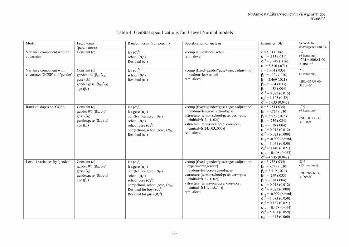
3.2 Three-level Normal models This set of data is a subset of the A-level data analysis project (1998~2001) of exams from establishments in England. The data consist of a score related to A-level results for ~31,000 individuals from 2,410 schools in 131 Local Education Authorities (LEA). The following fields were loaded into a GenStat spreadsheet. The variable name within GenStat, and type of variable (factor = categorical variable, or variate = quantitative variable) are shown after the description. • Individual ID (indiv, factor) • Age in months, centered about 18.5 years (age, variate) • Gender (gender, factor with male=0, female=1) • GCSE average score, centered about its mean value (gcse, variate) • A-level score classified as 0,2,4,6,8,10 (alevel, variate) • School (school, factor) • LEA ID (lea, factor) This example data is very large, and is useful to test the efficiency of the algorithm. Summaries of the analysis are given in Table 4. Note the use of the option CADJUST=no to suppress any further centering of covariates. 3.3 Two-level models for binary data These data come from the 1988 Bangladesh Fertility Survey and consist of a subsample of 1934 women grouped in 60 districts. The variables were loaded into a GenStat spreadsheet and defined as follows: • identifying code for each woman (woman, factor) • identifying code for each district (district, factor) • indicator of contraceptive use status at time of survey: response variable, 1=using contraception,

0=not using contraception • number of living children at time of survey, classified as none, one, two, three or more (nchild,

factor) • age of woman at time of survey (in years), centered around mean (cage, variate) • type of region of residence, 1=urban, 2=rural (region, factor) Generalised linear mixed models can be fitted using procedures. These are programs (written in the GenStat command language) that do not form part of the core code, but are supplied with the program, and are covered by the documentation. The GLMM procedure provides the PQL and MQL methods of Breslow and Clayton for simple variance components models. A set of procedures (HGFIXED, HGRANDOM, HGANALYSE) are available to fit the hglm models of Lee and Nelder, including mean/dispersion modelling. A simple analysis is given in Table 5. Random coefficient models cannot be fitted directly for non-normal mixed models, but can be fitted indirectly as a variance components model using suitable covariates.

-7-


Table 4. GenStat specifications for 3-level Normal models

Model Fixed terms


convergence and RL Variance component without covariates

Constant (c) lea (σ12)

school (σ22)

Residual (σ2)

vcomp random=lea+school reml alevel

c = 5.31 (0.06) σ1

2 = .153 (.051) σ2

2 = 2.749 (.116) σ2 = 8.516 (.071)

1.2 (6 iterations) -2RL=100861.00, 31081 df

Variance component with covariates 'GCSE' and 'gender'

Constant (c) gender 1/2 (β11/β12) gcse (β2) gender.gcse (β31/β32) age (β4)

lea (σ12)

school (σ22)

Residual (σ2)

vcomp [fixed=gender*gcse+age; cadjust=no] random=lea+school reml alevel

c = 5.964 (.035) β11 = -.734 (.030) β2 = 2.469 (.021) β32 = .264 (.033) β4 = -.038 (.004) σ1

2 = 0.022 (0.015) σ2

2 = 1.125 (0.52) σ2 = 5.033 (0.042)

2.0 (6 iterations) -2RL=83959.00, 31014 df

Random slopes on 'GCSE' Constant (c) gender 0/1 (β10/β11) gcse (β2) gender.gcse (β31/β32) age (β4)

lea (σ12)

lea.gcse (σ22)

corr(lea, lea.gcse) (σ12) school (σ3

2) school.gcse (σ4

2) corr(school, school.gcse) (σ34) Residual (σ2)

vcomp [fixed=gender*gcse+age; cadjust=no] random=lea/gcse+school/gcse vstructure [terms=school/gcse; corr=pos; cinitial=!(.2,-.1,.02)] vstructure [terms=lea/gcse; corr=pos; cinitial=!(.24,-.03,.005)] reml alevel

c = 5.954 (.034) β11 = -.734 (.030) β2 = 2.523 (.028) β32 = .259 (.034) β4 = -.038 (.004) σ1

2 = 0.018 (0.012) σ2

2 = 0.023 (0.009) σ12 = -0.999 (bound) σ3

2 = 1.071 (0.050) σ4

2 = 0.140 (0.021) σ34 = -0.498 (0.063) σ2 = 4.935 (0.042)

17.0 (6 iterations) -2RL=83730.33, 31010 df

Level 1 variances by 'gender' Constant (c) gender 0/1 (β10/β11) gcse (β2) gender.gcse (β31/β32) age (β4)

lea (σ12)

lea.gcse (σ22)

corr(lea, lea.gcse) (σ12) school (σ3

2) school.gcse (σ4

2) corr(school, school.gcse) (σ34) Residual for boys (σb

2) Residual for girls (σg

2)

vcomp [fixed=gender*gcse+age; cadjust=no; experiment=gender] random=lea/gcse+school/gcse vstructure [terms=school/gcse; corr=pos; cinitial=!(.2,-.1,.02)] vstructure [terms=lea/gcse; corr=pos; cinitial=!(1.1,-.15,.14)] reml alevel

c = 5.952 (.034) β11 = -.749 (.030) β2 = 2.519 (.029) β32 = .259 (.033) β4 = -.038 (.004) σ1

2 = 0.018 (0.012) σ2

2 = 0.023 (0.009) σ12 = -0.999 (bound) σ3

2 = 1.083 (0.050) σ4

2 = 0.137 (0.021) σ34 = -0.478 (0.064) σb

2 = 5.161 (0.059) σg

2 = 4.645 (0.060)

25.9 (13 iterations) -2RL=86667.3, 31009 df

-8-


Ordinal multinomial model, variance components with covariates 'GCSE' and 'gender' (see section 4.4)

Constant (c) gender 1/2 (β11/β12) gcse (β2) gender.gcse (β31/β32) age (β4)

lea (σ12)

school (σ22)

Residual (σ2)

irclass [prin=model,comp,eff; fixed=gcse*gender+age; random=lea+school; method=ai] yclass=alevel/2

c = 3.313 (.029) β11 = -.645 (.025) β2 = 2.106 (.022) β32 = .217 (.030) β4 = -.033 (.003) σ1

2 = 0.014 (0.010) σ2

2 = 0.793 (0.037) σ2 = 1.0 (fixed)

211.7 (8 iterations)

Table 5 GenStat specifications for 2-level logistic model

Model Fixed terms


convergence Variance component with all two covariates - logistic link, PQL method

Constant (c) nchild 1/2/3/4 (β11/β12/β13/β14) cage (β2) region (β31/β32)

district (σ12)

dispersion (ϕ) glmm [fixed=nchild+cage+region; random=district; dist=binomial] use; nbinomial=1

c = -1.667 (0.146) β12 = 1.09 (0.15) β12 = 1.35 (0.17) β12 = 1.32 (0.18) β2 = -0.026 (.008) β32 = 0.720 (0.118) σ1

2 = 0.211 (0.070) ϕ = 1 (fixed)

1.5 (5 iterations)

-9-


Table 6 GenStat specifications for multilevel Poisson model

Model Fixed terms(parameter/s)

Random terms (component) Specification of analysis Estimates (SE) Seconds to convergence

2-level variance components with the covariate UBV index, PQL method

Constant (c) uvbi (β1)

region (σ22)

dispersion (ϕ) glmm [fixed=uvbi; cadjust=no; random=nation+region; offset=logexp; dist=poisson] obs

c = -0.131 (.050) β1 = -0.034 (.010) σ2

2 = 0.173 (.031) ϕ = 1 (fixed)

0.5 (5 iterations)

2-level variance components with the covariate UBV index, PQL method, dispersion estimated


region (σ22)

dispersion (ϕ) glmm [fixed=uvbi; cadjust=no; random=nation+region; offset=logexp; dist=poisson; disp=*] obs

c = -0.129 (.050) β1 = -0.038 (.010) σ2

2 = 0.166 (.031) ϕ = 1.289 (.109)

0.2 (5 iterations)

3-level variance components with the covariate UBV index, PQL method


nation (σ12)

region (σ22)

dispersion (ϕ)

glmm [fixed=uvbi; cadjust=no; random=nation+region; offset=logexp; dist=poisson] obs

c = -0.057 (.141) β1 = -0.028 (.011) σ1

2 = 0.156 (.141) σ2

2 = 0.049 (.011) ϕ = 1 (fixed)

0.3 (4 iterations)

3-level variance components with the covariate UBV index, PQL method, dispersion estimated


nation (σ12)

region (σ22)

dispersion (ϕ)

glmm [fixed=uvbi; cadjust=no; random=nation+region; offset=logexp; dist=poisson; disp=*] obs

c = -0.061 (.140) β1 =- 0.031 (.011) σ1

2 = 0.153 (.086) σ2

2 = 0.045 (.011) ϕ = 1.284 (.108)

0.3 (5 iterations)

3-level variance components with the covariate UBV index, PQL method, negative binomial distribution with parameter φ


nation (σ12)

region (σ22)

dispersion (ϕ)

irreml [fixed=uvbi; cadjust=no; random=nation+region; initial=0.15,0.05; offset=logexp; distribution=negativebinomial; disp=1] obs

c = -0.072 (.138) β1 = -0.033 (.011) σ1

2 = 0.147 (.083) σ2

2 = 0.042 (.010) ϕ = 1 (fixed) φ = 0.013

1.4 (10 iterations)

3-level variance components with the covariate UBV index, PQL method, negative binomial distribution with parameter φ, dispersion estimated


nation (σ12)

region (σ22)

dispersion (ϕ)

irreml [fixed=uvbi; cadjust=no; random=nation+region; initial=0.15,0.05; offset=logexp; distribution=negativebinomial; disp=1] obs

c = -0.072 (.138) β1 = -0.033 (.011) σ1

2 = 0.147 (.083) σ2

2 = 0.042 (.011) ϕ = 0.990 (0.084) φ = 0.013

0.9 (6 iterations)

-10-


3.4 Three/two-level models for count data This set of data comes from the study of Malignant Melanoma Mortality in the European Community associated with the impact of UV radiation exposure. The data has a three-level structure with county nested within region nested within nation. The following variables were loaded into a GenStat spreadsheet: • Nation (1=Belgium, 2 = W.Germany, 3 = Denmark, 4 = France, 5 = UK, 6 = Italy, 7 = Ireland,

8 = Luxembourg, 9 = Netherlands) (nation, factor) • Region ID (region, factor) • County ID (county, factor) • Number of male deaths due to MM during 1971~ 1980 (obs, response variate) • Number of expected deaths (exp, variate) • Constant vector of 1 (cons, variate) • Measure of the UVB dose reaching the earth's surface in each county and centered (uvbi,

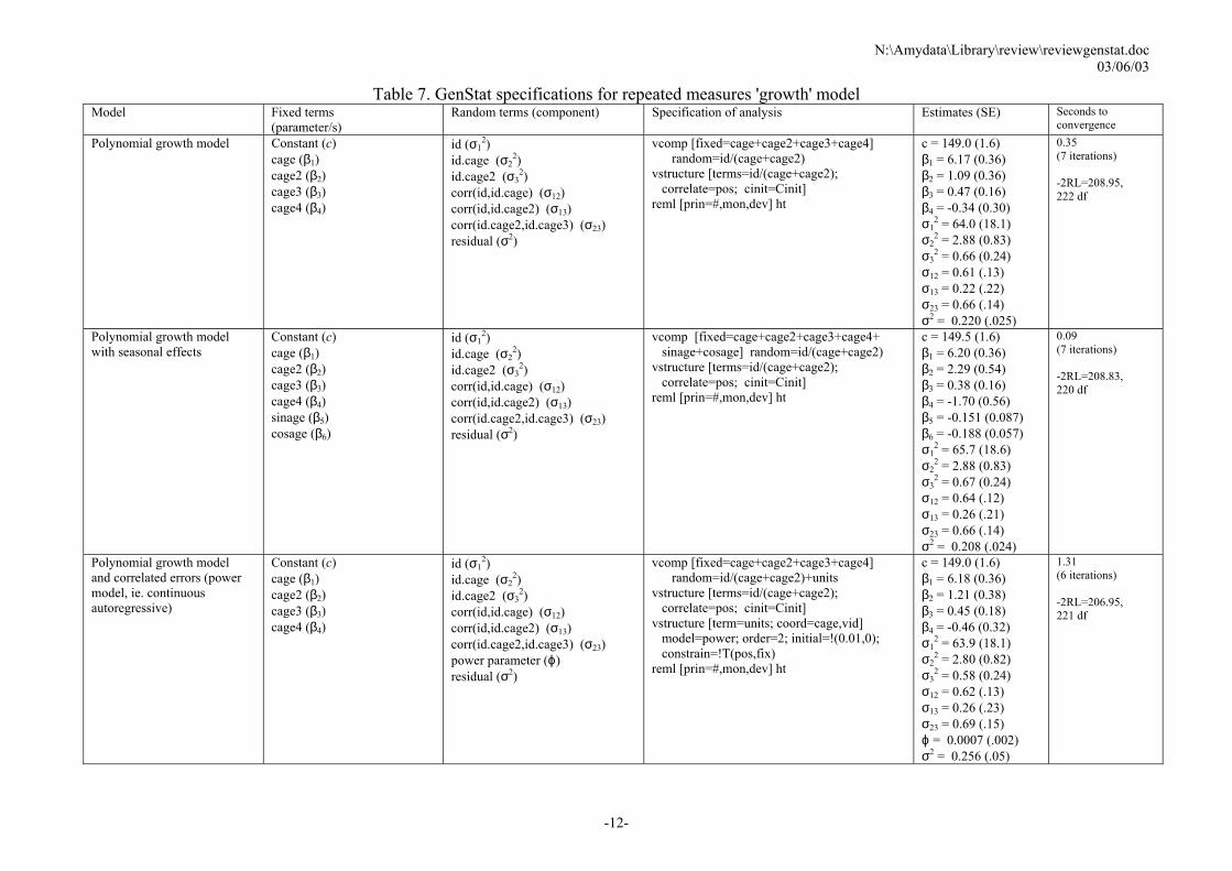
variate) The variable log(exp) is used as an offset variable. A summary of various analyses using either the Poisson or negative binomial distribution is given in Table 6. The PQL method is used for analysis. 3.5 Growth type models for repeated measures data

A wide range of time series correlation structures are available for multilevel mixed models in GenStat, including uniform, autoregressive, power (continuous autoregressive) moving average, banded and unstructured. All of the correlation structures can be fitted with constant or changing variance across time. In addition, several covariance structures are available: diagonal (independent heterogeneous), antedependence (generalized autoregressive model), factor-analytic or unstructured.

Measurements on height of 26 boys were taken on 9 occasions between the ages of 11 and 13 years for each of them. The measurements are approximately 0.25 year apart. The data variables were loaded in to a GenStat spreadsheet with the following definitions:

• Individual ID (id, factor) • Age in years, centred at 12 years (cage, variate) • Height in cm (ht, variate) • Occasion number (occ, factor) • Season in decimal year (partofyear, variate)

Several analyses are shown in Table 7. The power model (continuous autoregressive model) takes account of the fact that measurements are not equally spaced. Note that the estimated parameter for the power model is dependent on the scale of the age variable. In this case the estimated value of 0.00075 is the correlation between measurements 1 year apart. A typical time between measurements is 0.2 years, so the correlation between adjacent measurements 0.2 years apart is 0.000750.2 = 0.237.

-11-


Table 7. GenStat specifications for repeated measures 'growth' model Model Fixed terms


convergence Polynomial growth model Constant (c)

cage (β1) cage2 (β2) cage3 (β3) cage4 (β4)

id (σ12)

id.cage (σ22)

id.cage2 (σ32)

corr(id,id.cage) (σ12) corr(id,id.cage2) (σ13) corr(id.cage2,id.cage3) (σ23) residual (σ2)

vcomp [fixed=cage+cage2+cage3+cage4] random=id/(cage+cage2) vstructure [terms=id/(cage+cage2); correlate=pos; cinit=Cinit] reml [prin=#,mon,dev] ht

c = 149.0 (1.6) β1 = 6.17 (0.36) β2 = 1.09 (0.36) β3 = 0.47 (0.16) β4 = -0.34 (0.30) σ1

2 = 64.0 (18.1) σ2

2 = 2.88 (0.83) σ3

2 = 0.66 (0.24) σ12 = 0.61 (.13) σ13 = 0.22 (.22) σ23 = 0.66 (.14) σ2 = 0.220 (.025)

0.35 (7 iterations) -2RL=208.95, 222 df

Polynomial growth model with seasonal effects

Constant (c) cage (β1) cage2 (β2) cage3 (β3) cage4 (β4) sinage (β5) cosage (β6)

id (σ12)

id.cage (σ22)

id.cage2 (σ32)

corr(id,id.cage) (σ12) corr(id,id.cage2) (σ13) corr(id.cage2,id.cage3) (σ23) residual (σ2)

vcomp [fixed=cage+cage2+cage3+cage4+ sinage+cosage] random=id/(cage+cage2) vstructure [terms=id/(cage+cage2); correlate=pos; cinit=Cinit] reml [prin=#,mon,dev] ht

c = 149.5 (1.6) β1 = 6.20 (0.36) β2 = 2.29 (0.54) β3 = 0.38 (0.16) β4 = -1.70 (0.56) β5 = -0.151 (0.087) β6 = -0.188 (0.057) σ1

2 = 65.7 (18.6) σ2

2 = 2.88 (0.83) σ3

2 = 0.67 (0.24) σ12 = 0.64 (.12) σ13 = 0.26 (.21) σ23 = 0.66 (.14) σ2 = 0.208 (.024)

0.09 (7 iterations) -2RL=208.83, 220 df

Polynomial growth model and correlated errors (power model, ie. continuous autoregressive)

Constant (c) cage (β1) cage2 (β2) cage3 (β3) cage4 (β4)

id (σ12)

id.cage (σ22)

id.cage2 (σ32)

corr(id,id.cage) (σ12) corr(id,id.cage2) (σ13) corr(id.cage2,id.cage3) (σ23) power parameter (ϕ) residual (σ2)

vcomp [fixed=cage+cage2+cage3+cage4] random=id/(cage+cage2)+units vstructure [terms=id/(cage+cage2); correlate=pos; cinit=Cinit] vstructure [term=units; coord=cage,vid] model=power; order=2; initial=!(0.01,0); constrain=!T(pos,fix) reml [prin=#,mon,dev] ht

c = 149.0 (1.6) β1 = 6.18 (0.36) β2 = 1.21 (0.38) β3 = 0.45 (0.18) β4 = -0.46 (0.32) σ1

2 = 63.9 (18.1) σ2

2 = 2.80 (0.82) σ3

2 = 0.58 (0.24) σ12 = 0.62 (.13) σ13 = 0.26 (.23) σ23 = 0.69 (.15) ϕ = 0.0007 (.002) σ2 = 0.256 (.05)

1.31 (6 iterations) -2RL=206.95, 221 df

-12-



4. Model specifications: other random effects models There is no restriction on the use of cross-classified factors within GenStat. GenStat can also fit general multivariate models, spatial models and factor analysis variance structures. In addition, it allows joint analysis of multiple experiments with different correlated error structures within each experiment. Menu-driven analysis is possible for standard models for general mixed models, repeated measurements data, random coefficient regression, spatial analysis or multivariate analysis. The menus calculate initial values where required by the models and the commands used are retained in the session log so an audit trail is available. In addition, users have access to the full range of models via the command language. 4.1 Spatial analysis There are facilities for spatial analysis of data laid out on a regular grid, or data sampled from irregular points in an area. Where data is laid out on a regular grid (as rows x columns), separable error structures are often fitted at the row.column level, ie. separate spatial models are assumed to act independently across rows and across columns. Any of the GenStat correlation models can be used to describe the pattern in each direction, and the direct product structure is used within the algorithm to give increased efficiency. In the case where data is not laid out on a regular grid, then a one- or two-parameter power model can be used to model the spatial pattern at the units level. 4.2 Multivariate analysis Multivariate analysis is performed by appending the variables into a single variate and using unstructured variance models to model the relationship between variables. Functions to manipulate data sets in this way and construct the necessary structural factors are available in the GenStat spreadsheet. 4.3 Joint analysis of several data sets Where several similar experiments have been carried out, it can be advantageous to carry out a joint analysis of the data sets to get a combined estimate of treatment effects. The REML facilities in GenStat include the ability to easily specify the separate experiments and define separate residual level models for each experiment. Any other random terms can also be included in the model. This feature was originally developed for joint analysis of a set of variety trials, each requiring a different spatial model, but is useful in a much wider context. 4.4 Ordered categorical data Ordered categorical (or ordinal multinomial) data can be fitted using the Biometris procedure IRCLASS, which is freely available from their website http://www.Biometris.nl/GenStat, complete with documentation. An example of analysis using this method was given for the A-level results data set in table 4. This analysis might be considered more appropriate for this data set as the A-level scores are classified as 0,2,4,6,8,10. The procedure analyses the score transformed onto the scale 0-6.

-14-

http://www.biometris.nl/GenStat


5. Documentation and user support Documentation on the GenStat system is available as hard copy or online from the help system within GenStat. The documentation consists of an overall guide to the system ‘GenStat for Windows’, and ‘The Guide to Genstat’ gives basic information on the underlying command language. The ‘GenStat Reference Manual’ gives a more detailed description of the system and statistical methods used, including a chapter on analysis of linear mixed models (multi-level models). The documents cannot be downloaded separately, but a 30-day fully functional demo version can be downloaded, including on-line documentation, from the VSN International website at http://www.vsn-intl.com/. This website also provides additional information and downloads for GenStat users, including information on how to join the GenStat user discussion list. In addition, a support service is available. These facilities in GenStat reviewed here are under continual development. The next version will contain general prediction for multilevel models and is currently being tested prior to release. 6. Contact details for the supplier GenStat is marketed by VSN International Ltd, 5 The Waterhouse, Waterhouse St, Hemel Hempstead, HP1 IES, UK. The VSN website can be found at http://www.vsn-intl.com/.

-15-

http://www.vsn-intl.com/

http://www.vsn-intl.com/

Documents

Software review – multilevel models in GenStat Sue …bristol.ac.uk/cmm/learning/mmsoftware/reviewgenstat.pdfN:\Amydata\Library\review\reviewgenstat.doc 03/06/03 Software review